57
Economics 325 Public Finance Martin Farnham University of Victoria Fall 2010
Economics 325 Public Finance
Martin Farnham University of Victoria
Fall 2010

Econ 325--Farnham 2
Course logistics
Professor: Martin Farnham [email protected] BEC 354 Office Hours: Tue 12:30-3:30
TA: Amy Hu
BEC 325 Office Hours: Thurs 3-4
Econ 325--Farnham 3
Course logistics (cont)
• Evaluation – Midterm 1, 25% (Tuesday Oct 5, in class) – Midterm 2, 25% (Friday Nov 5, in class) – Final Exam 50% (details TBA)
• Text: Rosen et al. “Public Finance in Canada” – Recommended, but not required. Old edition on
reserve (shortly). • Assignments
– Ungraded problem sets – Readings assigned occasionally

Econ 325--Farnham 4
Course Logistics (cont)
• Attendance – If miss every one of first three classes,
automatically dropped (else notify me) – Technically attendance not required;
however, strongly recommended. – You are responsible for anything you miss – Lecture notes posted, but not necessarily
complete

Econ 325--Farnham 5
Course logistics (cont)
• Office hours – Use them!!
• Learning in this course – Do readings – Keep good notes – MOST importantly, do problem sets carefully and
thoroughly – Think!
• See syllabus for additional details

Econ 325--Farnham 6
A note on email etiquette
• Please don’t email me about – Information available elsewhere (course website,
course outline, etc.) – What you missed if you skipped a lecture – What’s going to be on an exam – Things you could ask me in office hours – I reserve the right to ignore emails that I deem
inappropriate • Please use the standard letter format
– Sign your email – Don’t use text message abbreviations (I won’t
understand them!)

Econ 325--Farnham 7
What is Public Finance?
• What it’s not – Corporate finance/banking – Macroeconomic fiscal policy
• What it is – Economics of the public sector – Study of what government should do, and
what effect government has at micro level

Econ 325--Farnham 8
The Role of Government in a Market Economy
Why might the government want to intervene in a market economy?
Four main reasons 1) Establish/maintain property rights 2) Correct market failures 3) Promote fairness/equity 4) Paternalism
Econ 325--Farnham 9
Property Rights
• Government establishes legal framework for economic interactions – Protects property rights
• Otherwise little incentive to create wealth; lots of resources diverted to defending ones assets against seizure
– Enforces contracts between individuals • Otherwise individuals are forced to rely on trust when
entering into agreements with others
• This aspect of government accounts for a relatively small fraction of total expenditures.
Econ 325--Farnham 10
Market Failure
• Under perfect competition (and ideal conditions), equilibrium Pareto-efficient
• Ideal conditions are pretty unrealistic; when these fail we likely have market failure
• In this case, government intervention can be Pareto-improving (or at least social welfare improving); can even lead to Pareto-efficient outcome
Econ 325--Farnham 11
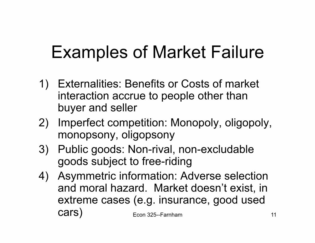
Examples of Market Failure
1) Externalities: Benefits or Costs of market interaction accrue to people other than buyer and seller
2) Imperfect competition: Monopoly, oligopoly, monopsony, oligopsony
3) Public goods: Non-rival, non-excludable goods subject to free-riding
4) Asymmetric information: Adverse selection and moral hazard. Market doesn’t exist, in extreme cases (e.g. insurance, good used cars)

Econ 325--Farnham 12
Fairness/Equity
• Recall it is Pareto Efficient to give everything to one person in society, and nothing to everyone else – Can have efficient outcomes with starvation – Probably not socially desirable
• Government can use taxes and expenditures in order to equalize income, consumption, or wealth; or to maintain minimum standard

Econ 325--Farnham 13
Paternalism • Principle of consumer sovereignty holds that
individuals know what is best for themselves • Paternalism goes against this principle
– Government sometimes tries to protect individuals from perceived ignorance or short-sightedness.
– e.g. Seatbelt laws, criminalization of drugs, mandatory education, laws against child labour, workplace safety standards

Econ 325--Farnham 14
Levels of Government
• Note that there are different levels of government in Canada, each with taxing and spending authority – Federal – Provincial – Municipal
• While much of our focus will be on the federal level, important functions occur at the provincial and local level
Econ 325--Farnham 15
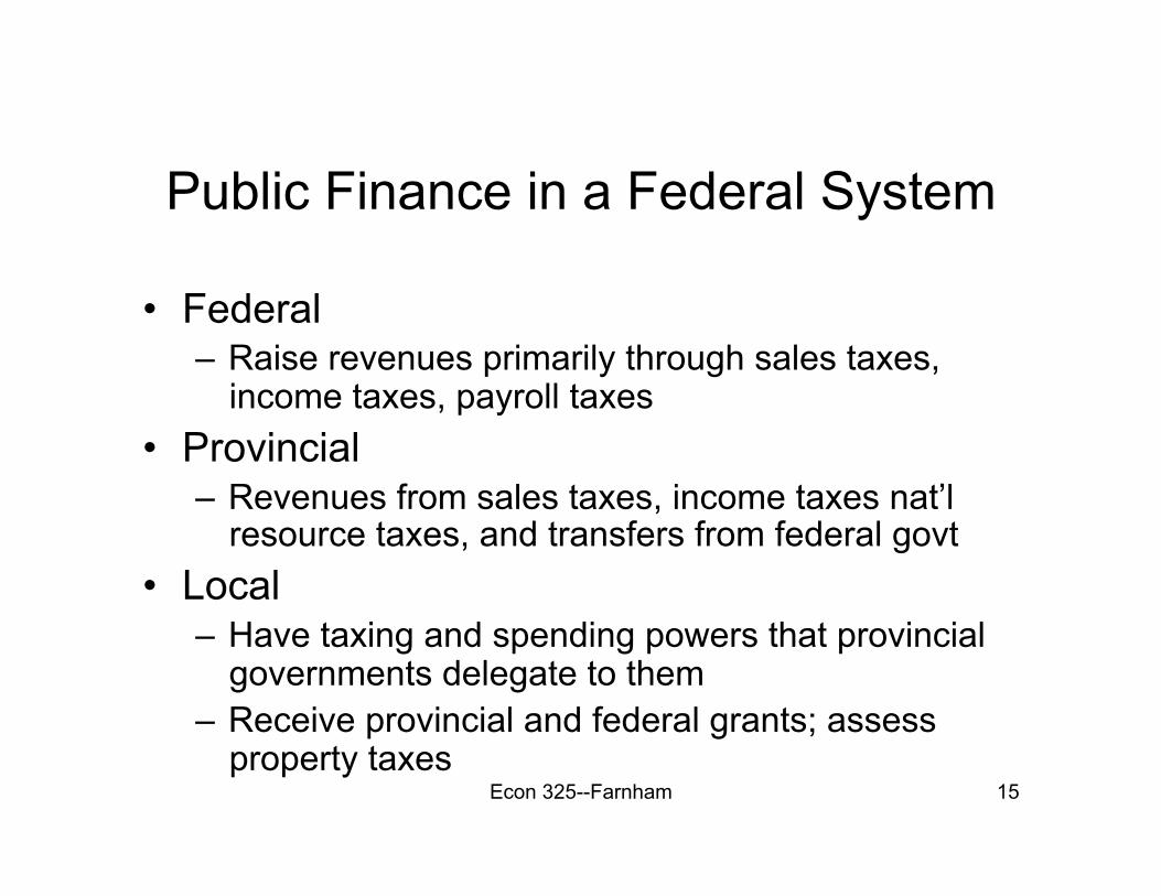
Public Finance in a Federal System
• Federal – Raise revenues primarily through sales taxes,
income taxes, payroll taxes • Provincial
– Revenues from sales taxes, income taxes nat’l resource taxes, and transfers from federal govt
• Local – Have taxing and spending powers that provincial
governments delegate to them – Receive provincial and federal grants; assess
property taxes

Econ 325--Farnham 16
Government Expenditures
• Education (primary, secondary, tertiary) • Public Assistance: Means-tested--
eligibility depends on income, assets – e.g. Welfare, housing assistance
• Social Insurance – e.g. Canada Pension Plan, Public Health,
Employment Insurance
Econ 325--Farnham 17
Govt Expenditures (cont)
• Infrastructure (e.g. transport, communication)
• Protection of persons, property • National defense • Various other
Econ 325--Farnham 18
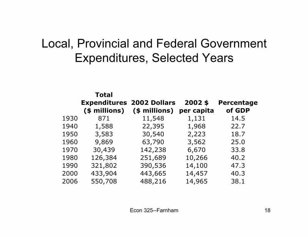
Local, Provincial and Federal Government Expenditures, Selected Years
Total Expenditures 2002 Dollars 2002 $ Percentage ($ millions) ($ millions) per capita of GDP
1930 871 11,548 1,131 14.5 1940 1,588 22,395 1,968 22.7 1950 3,583 30,540 2,223 18.7 1960 9,869 63,790 3,562 25.0 1970 30,439 142,238 6,670 33.8 1980 126,384 251,689 10,266 40.2 1990 321,802 390,536 14,100 47.3 2000 433,904 443,665 14,457 40.3 2006 550,708 488,216 14,965 38.1

Econ 325--Farnham 19
Government Expenditures in 2008 (%GDP) International Comparison
Expenditures as a Country Percentage of GDP Canada 39.7 France 52.7 Germany 44.0 Italy 48.7 Japan 37.1 United States 39.0 United Kingdom 48.1

Econ 325--Farnham 20
Expenditures by Function All Levels of Government
Function 1933 2006 Health 3.7 21.2 Social Welfare 14 23.3 Education 11.3 14.9 Transportation and communications 9.4 4.1 Debt charges 31.5 8.5 Other 30.2 28 Total 100 100

Econ 325--Farnham 21
Government Revenues
• Revenues in Canada in 2006 came from a variety of sources including – Personal income tax (32.3%) – Corporate income tax (10.4%) – Public pension contributions, payroll taxes (8.4%) – Customs, excises, and sales taxes (19.2%) – Property taxes (9.2%) – Investment income (8.1%) – Other (12.4%)

Econ 325--Farnham 22
Brief Outline of Course
• Review micro theory • Discuss theoretical and empirical methods of
analysis in Public Finance • Discuss role of government in economy • Analysis of government expenditures in
Canada • Discuss effects of taxation • Analysis of taxation in Canada • Possibly some discussion of collective choice
mechanisms (e.g. voting) at end

Econ 325--Farnham 23
Review of Microeconomics • Reading for Micro Review
– Your principles of micro text and/or notes – Rosen Chapter 2 appendix
• Analyzing market outcomes 1) with an interest in policy that will correct market failures when such failures occur; and 2) with an interest in the costs associated with redistributive or paternalistic policy
• Primary questions throughout: – To what outcomes do markets lead? – Under what circumstances are these outcomes desirable? – If markets outcomes are undesirable, what would be the
desirable outcome? What is the correct policy response?

Econ 325--Farnham 24
Review of Microeconomics • Analyzing what happens involves positive analysis
• Terms desirable and undesirable imply we are also interested in normative analysis.
• Positive analysis involves asking what an outcome will be under certain circumstances: – Ex: in equilibrium, how carbon will drivers emit?
• Normative analysis involves asking questions about what outcomes we would like to see. (what should be) – Ex: what is the right (socially optimal) amount of carbon
emissions?
• Points to the need for a normative criterion by which to judge outcomes as “good” or “bad”.
Econ 312--Farnham 25
Review of Microeconomics • Normative criterion we use in economics is typically that of
economic efficiency.
• Important to keep in mind that economic efficiency
– has utilitarianism as its philosophical base – says nothing (much) about fairness or equity – is only one of many criteria that we can (should?) use to
judge market outcomes.
• With these caveats in mind, in this class we will (usually) judge outcomes in terms of whether or not they are economically efficient. – Normative statements like “outcome X should happen”
should be read as shorthand for “outcome X should happen if we are using economic efficiency as the sole criterion for decision-making.”

26
Review of Microeconomics • Economic efficiency defined:
– An outcome is efficient if it maximizes net benefits, where net benefits are equal to total benefits minus total costs.
• Tells us that, at its core, the analysis of economic efficiency is simply cost-benefit analysis.
• We will be analyzing efficiency in a variety of contexts, such as: 1. What is the efficient level of provision of a public service?
• Ex: what is the efficient level of C02 emission? 3. Should we undertake a particular project (binary decision-
making)? • Ex: should BC put on the Olympics?
5. How should we allocate a scarce resource across competing uses? • Ex: Should Bear Mountain remain open space, be developed
as a golf course/condo project or be used for agriculture?

Econ 312--Farnham 27
Review of Microeconomics • We will focus on answering questions such as these by using cost-
benefit analysis to identify the outcomes that make net benefits as large as possible.
• Important point: we need to make sure we have correctly identified and measured all of the costs and benefits associated with a given activity/outcome.
• An alternative characterization of efficiency (that we may pick up on at various points throughout the term):
– An outcome is efficient is it is impossible to come up with an alternative outcome in which at least one person can be made better off without any one person being made worse off.
• Although it may not be immediately obvious, we will see that this characterization of efficiency will be satisfied if net benefits are maximized.

Econ 312--Farnham 28
Review of Microeconomics • In order to answer normative questions such as those posed
above, we first need to understand how to answer positive questions.
– For instance, we need to understand what market outcomes look like, in order to work out whether they are desirable (efficient).
• This means we need to recall some basic ideas we learned in principles of microeconomics.
• Specifically, we want to understand: 1. How consumers decide what goods to buy (demand). 2. How producers decide what goods to produce (supply). 3. How markets bring producers and consumers together
(equilibrium).
• Once we understand this, we can assess whether consumers and producers act in such a way as to achieve an economically efficient outcome.
Econ 312--Farnham 29
Review of Microeconomics 1. Review of Demand.
• Three areas to cover on the demand side: i. Interpreting an individual consumer’s demand curve ii. Measuring consumer well-being using the demand curve iii. Deriving aggregate demand from individual demand
Econ 312--Farnham 30
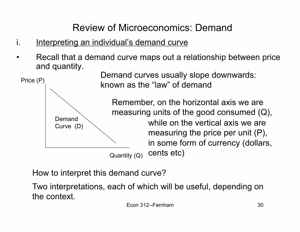
Review of Microeconomics: Demand i. Interpreting an individual’s demand curve
• Recall that a demand curve maps out a relationship between price and quantity.
Price (P)
Quantity (Q)
Demand curves usually slope downwards: known as the “law” of demand
while on the vertical axis we are measuring the price per unit (P), in some form of currency (dollars, cents etc)
Remember, on the horizontal axis we are measuring units of the good consumed (Q),
How to interpret this demand curve? Two interpretations, each of which will be useful, depending on the context.
Demand Curve (D)

Econ 312--Farnham 31
Review of Microeconomics: Demand
• The first interpretation of the demand curve is probably the most familiar to you:
P
Q
Interpretation 1: the D curve tells us how many units of a good a consumer wishes to buy in total, at a given price per unit for the good.
For instance, the D curve tells us that if the price per unit is P1, then the consumer would like to buy Q1 units.
We can think of this interpretation as reading the D curve horizontally: that is, if we plug in values for P, we get out values for Q.
D
P1
Q1
etc. Q2
P2
32
Review of Microeconomics: Demand
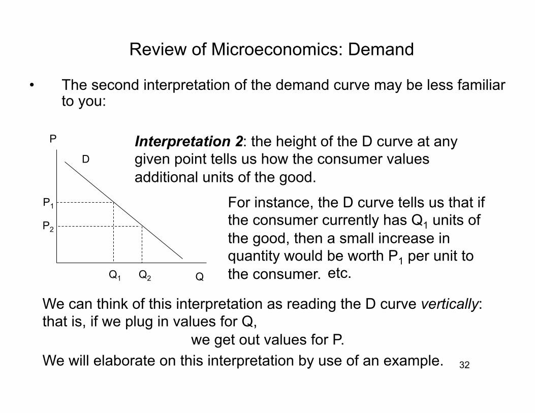
• The second interpretation of the demand curve may be less familiar to you:
P
Q
Interpretation 2: the height of the D curve at any given point tells us how the consumer values additional units of the good.
For instance, the D curve tells us that if the consumer currently has Q1 units of the good, then a small increase in quantity would be worth P1 per unit to the consumer.
D
P1
Q1 etc. Q2
P2
We can think of this interpretation as reading the D curve vertically: that is, if we plug in values for Q, we get out values for P. We will elaborate on this interpretation by use of an example.
Econ 312--Farnham 33
Review of Microeconomics: Demand
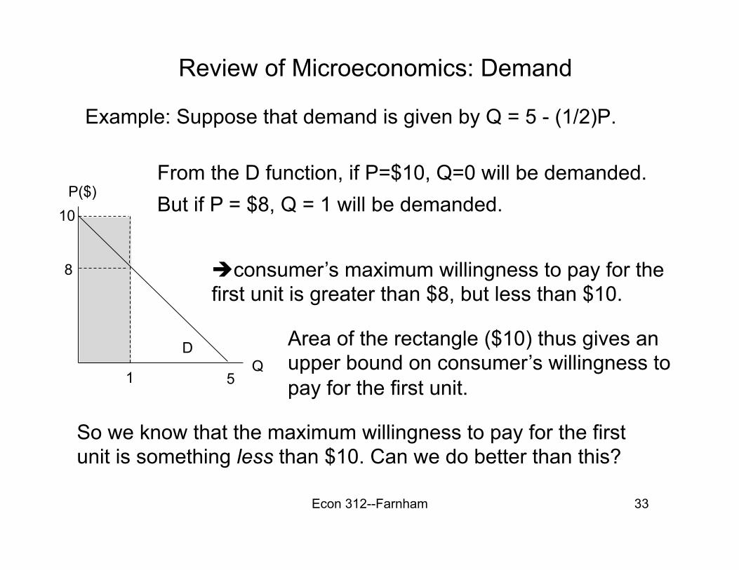
Example: Suppose that demand is given by Q = 5 - (1/2)P.
P($)
Q
From the D function, if P=$10, Q=0 will be demanded. But if P = $8, Q = 1 will be demanded.
consumer’s maximum willingness to pay for the first unit is greater than $8, but less than $10.
D
10
5
So we know that the maximum willingness to pay for the first unit is something less than $10. Can we do better than this?
Area of the rectangle ($10) thus gives an upper bound on consumer’s willingness to pay for the first unit. 1
8

Econ 312--Farnham 34
Review of Microeconomics: Demand Now consider smaller changes in P. Say P from $10 to $9 so that Q from 0 to 0.5.
P($)
Q
Consumer did not buy the first half unit when it cost $5, but does when it costs $4.50.
consumer’s maximum willingness to pay for this first half unit is something less than $5.
D
10
0.5
Now suppose P from $9 to $8, so that total Q from 0.5 to 1.
Consumer did not buy the second half unit when it cost $4.50, but does when P falls.
1 5
9 8
consumer’s maximum willingness to pay for this second half unit is something less than $4.50. This tells us that the consumer’s maximum willingness to pay for the first unit is in fact something less than $9.50 (as opposed to $10).

35
Review of Microeconomics: Demand We could consider even smaller changes in prices and quantities.
P($)
Q
For instance we could now lower the price in $0.50 increments, rather than in $1.00 increments.
Doing this allows us to see that the consumer’s maximum willingness to pay for the first unit is something less than $9.25.
D
10
9
8
0.5 1 5
In the limit, as we consider smaller and smaller price changes, what we are doing here is calculating the area under the demand curve between Q=0 and Q=1.
This area tells us the exact maximum willingness to pay by this consumer for the first unit of the good. In this case, the area of that trapezoid is equal to $9. The consumer is willing to pay at most $9 for the first unit.
Econ 312--Farnham 36
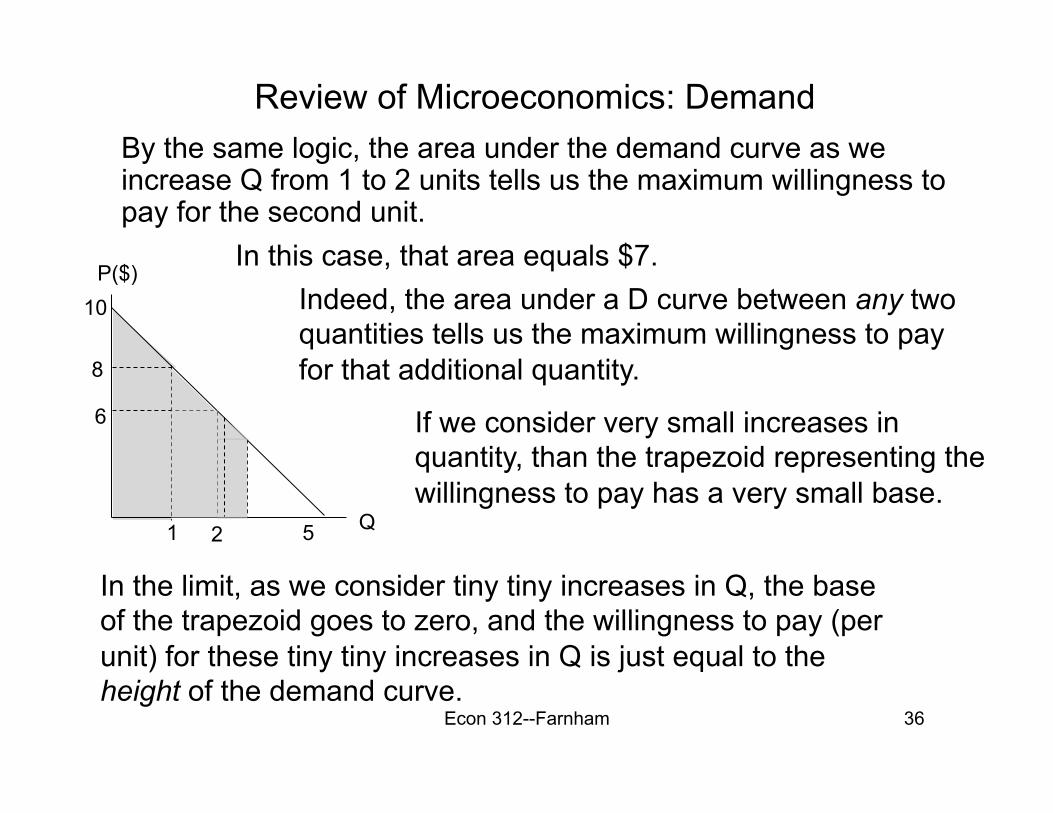
Review of Microeconomics: Demand By the same logic, the area under the demand curve as we increase Q from 1 to 2 units tells us the maximum willingness to pay for the second unit.
P($)
Q
In this case, that area equals $7.
10
1 5
Indeed, the area under a D curve between any two quantities tells us the maximum willingness to pay for that additional quantity.
In the limit, as we consider tiny tiny increases in Q, the base of the trapezoid goes to zero, and the willingness to pay (per unit) for these tiny tiny increases in Q is just equal to the height of the demand curve.
2
6 If we consider very small increases in quantity, than the trapezoid representing the willingness to pay has a very small base.
8
Econ 312--Farnham 37
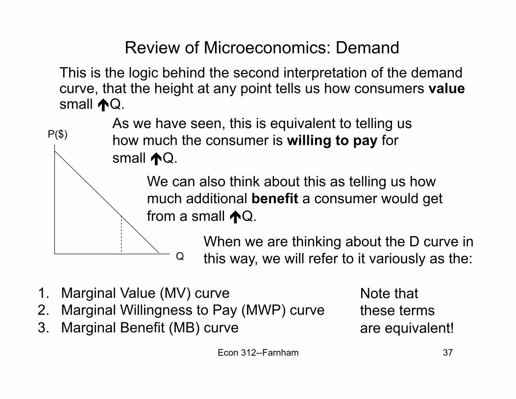
Review of Microeconomics: Demand This is the logic behind the second interpretation of the demand curve, that the height at any point tells us how consumers value small Q.
P($)
Q
As we have seen, this is equivalent to telling us how much the consumer is willing to pay for small Q.
When we are thinking about the D curve in this way, we will refer to it variously as the:
We can also think about this as telling us how much additional benefit a consumer would get from a small Q.
1. Marginal Value (MV) curve 2. Marginal Willingness to Pay (MWP) curve 3. Marginal Benefit (MB) curve
Note that these terms are equivalent!

Econ 312--Farnham 38
Review of Microeconomics: Demand ii. Measuring consumer well-being using the demand curve.
P($)
Q
1st interpretation of D curve: tells us Q demanded at a given P.
But, how much did consumer actually have to pay for Q1?
2nd interpretation of D curve: area under the D curve measures consumer’s willingness to pay for Q1 units.
Definition: consumer surplus (CS) = what a consumer is willing to pay minus what they have to pay.
P1
Q1
Expenditure (price times quantity) given by area P1Q1.
consumer willing to pay more than she has to pay.
Difference between willingness to pay and expenditure measures consumer well-being.
In the diagram above, the CS from buying Q1 units at P1 per unit is equal to the triangle A.
A
Econ 312--Farnham 39
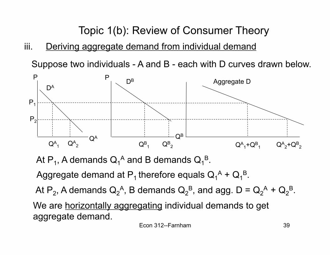
Topic 1(b): Review of Consumer Theory iii. Deriving aggregate demand from individual demand
P
QA
Suppose two individuals - A and B - each with D curves drawn below.
At P1, A demands Q1A and B demands Q1
B.
P1
QA1
We are horizontally aggregating individual demands to get aggregate demand.
DA
QB
QB1
DB
QA1+QB
1 QA2 QB
2 QA2+QB
2
Aggregate D
P2
Aggregate demand at P1 therefore equals Q1A + Q1
B.
At P2, A demands Q2A, B demands Q2
B, and agg. D = Q2A
+ Q2B.
P
Econ 312--Farnham 40
Topic 1: Introduction and Review 1. Review of Supply.
• Three areas to cover on the supply side: i. Interpreting an individual producer’s supply curve ii. Measuring producer well-being using the supply curve iii. Deriving aggregate supply from individual supply

Econ 312--Farnham 41
Topic 1: Introduction and Review: Supply i. Interpreting a firm’s supply curve
• Recall that a supply curve maps out a relationship between price and quantity.
Price (P)
Quantity (Q)
Supply curves usually slope upwards: known as the “law” of supply
i.e., firms that take the prices of output and inputs as given.
NB: Throughout this class we will only be looking at the supply behavior of competitive firms.
How to interpret this supply curve? Like D curve, there are two interpretations of the S curve.
Supply Curve (S)

Econ 312--Farnham 42
Topic 1: Introduction and Review: Supply
• The first interpretation of the supply curve is (again) probably most familiar:
P
Q
Interpretation 1: S curve tells us how many units of a good a producer wishes to sell in total, at a given price per unit for the good.
If the price per unit is P1, then the firm would like to sell Q1 units. etc, etc.
We can think of this interpretation as reading the S curve horizontally: that is, if we plug in values for P, we get out values for Q.
S
P1
Q1

Topic 1: Introduction and Review: Supply
• The second interpretation of the supply curve should also be (relatively) familiar:
P
Q
Interpretation 2: the height of the S curve at any given point tells us how much additional units of the good cost to produce.
i.e., the supply curve is also a Marginal Cost (MC) curve.
If the firm is currently producing Q1 units of the good, then a small increase in quantity would cost P1 per unit to produce.
S P1
Q1
We can think of this interpretation as reading the S curve vertically: that is, if we plug in values for Q, we get out values for P. Again, useful to work through an example.
Econ 312--Farnham 44
Topic 1: Introduction and Review: Supply
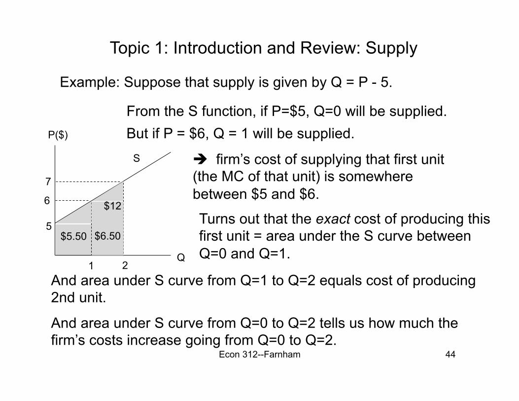
Example: Suppose that supply is given by Q = P - 5.
P($)
Q
From the S function, if P=$5, Q=0 will be supplied. But if P = $6, Q = 1 will be supplied.
firm’s cost of supplying that first unit (the MC of that unit) is somewhere between $5 and $6.
S
And area under S curve from Q=1 to Q=2 equals cost of producing 2nd unit.
And area under S curve from Q=0 to Q=2 tells us how much the firm’s costs increase going from Q=0 to Q=2.
Turns out that the exact cost of producing this first unit = area under the S curve between Q=0 and Q=1.
1
5
6
7
2
$5.50 $6.50
$12
Econ 312--Farnham 45
Topic 1: Introduction and Review: Supply
• Area under S curve up to a given Q actually tells us the Variable Cost (VC) of producing that Q.
• Recall that a firm’s Total Costs (TC) have 2 components: TC = Fixed Costs + Variable Costs
= FC + VC.
• By definition, FC don’t change as Q changes, while VC do.
• So MC = ΔTC/ΔQ = Δ (FC+VC) /ΔQ = ΔVC /ΔQ.
area under the S curve up to a given Q = MC of 1st unit + MC of 2nd unit + MC of third unit etc. etc.
• And adding up MCs is the same as calculating VC.

Econ 312--Farnham 46
Topic 1: Introduction and Review: Supply ii. Measuring producer well-being using the supply curve.
P($)
Q
1st interpretation of S curve: tells us Q supplied at a given P.
If producer sells Q1 units at P1 per unit, then Total Revenue (TR) received = area of rectangle P1Q1.
2nd interpretation of S curve: area under S curve measures VC of producing Q1 units.
Definition: producer surplus (PS) = TR - VC.
P1
Q1
producer receives revenue greater than VC.
Difference between TR and VC provides a measure of producer well-being.
In the diagram above, the PS from selling Q1 units at P1 per unit is equal to the triangle A.
A
Econ 312--Farnham 47
Topic 1: Introduction and Review: Supply
ii. Measuring producer well-being using the supply curve.
• More common measure of producer well-being is profit (π). – What is the relationship between PS and π?
• Recall:
PS = TR - VC; and
π = TR - TC π = TR - VC - FC
PS π = PS - FC
or PS = π + FC.
Econ 312--Farnham 48
Topic 1: Introduction and Review: Supply
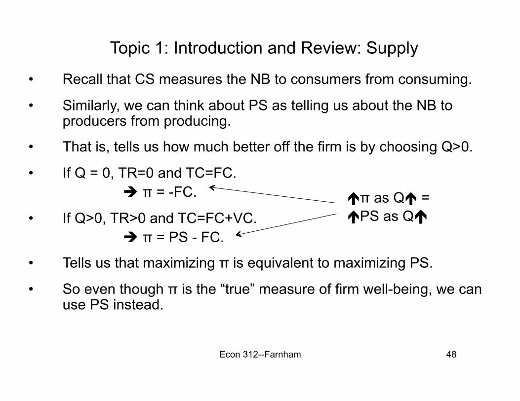
• Recall that CS measures the NB to consumers from consuming.
• Similarly, we can think about PS as telling us about the NB to producers from producing.
• That is, tells us how much better off the firm is by choosing Q>0.
• If Q = 0, TR=0 and TC=FC. π = -FC.
• If Q>0, TR>0 and TC=FC+VC. π = PS - FC.
• Tells us that maximizing π is equivalent to maximizing PS.
• So even though π is the “true” measure of firm well-being, we can use PS instead.
π as Q = PS as Q
Econ 312--Farnham 49
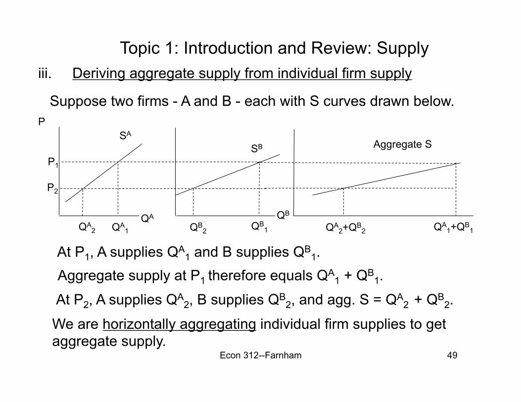
Topic 1: Introduction and Review: Supply iii. Deriving aggregate supply from individual firm supply
P
QA
Suppose two firms - A and B - each with S curves drawn below.
At P1, A supplies QA1 and B supplies QB
1.
P1
QA1
We are horizontally aggregating individual firm supplies to get aggregate supply.
SA
QB
QB1
SB
QA1+QB
1 QA2 QB
2 QA2+QB
2
Aggregate S
P2
Aggregate supply at P1 therefore equals QA1 + QB
1.
At P2, A supplies QA2, B supplies QB
2, and agg. S = QA2 + QB
2.
Econ 312--Farnham 50
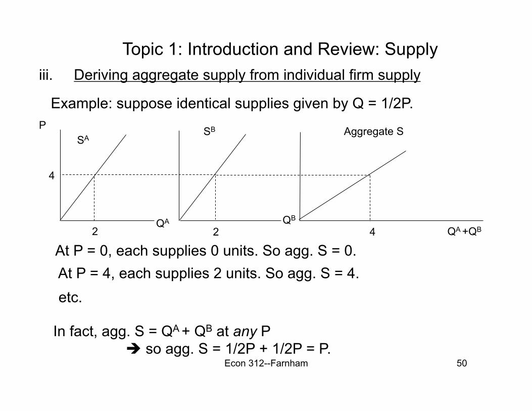
Topic 1: Introduction and Review: Supply iii. Deriving aggregate supply from individual firm supply
P
QA
Example: suppose identical supplies given by Q = 1/2P.
At P = 0, each supplies 0 units. So agg. S = 0. 2
In fact, agg. S = QA + QB at any P so agg. S = 1/2P + 1/2P = P.
SA
QB
2
SB
4
Aggregate S
4
At P = 4, each supplies 2 units. So agg. S = 4. etc.
QA +QB
Econ 312--Farnham 51
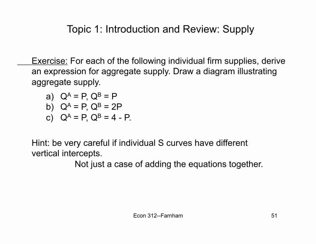
Topic 1: Introduction and Review: Supply
Exercise: For each of the following individual firm supplies, derive an expression for aggregate supply. Draw a diagram illustrating aggregate supply.
a) QA = P, QB = P b) QA = P, QB = 2P c) QA = P, QB = 4 - P.
Hint: be very careful if individual S curves have different vertical intercepts. Not just a case of adding the equations together.
Econ 312--Farnham 52
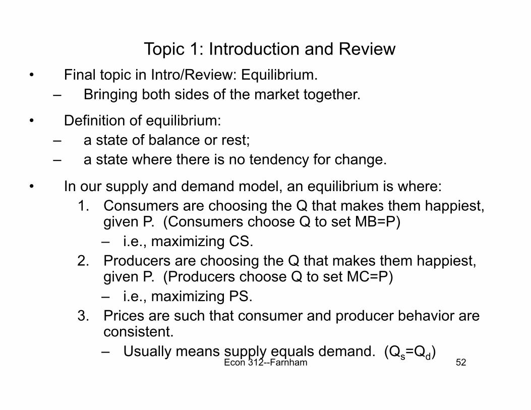
Topic 1: Introduction and Review • Final topic in Intro/Review: Equilibrium.
– Bringing both sides of the market together.
• Definition of equilibrium: – a state of balance or rest; – a state where there is no tendency for change.
• In our supply and demand model, an equilibrium is where: 1. Consumers are choosing the Q that makes them happiest,
given P. (Consumers choose Q to set MB=P) – i.e., maximizing CS.
2. Producers are choosing the Q that makes them happiest, given P. (Producers choose Q to set MC=P) – i.e., maximizing PS.
3. Prices are such that consumer and producer behavior are consistent. – Usually means supply equals demand. (Qs=Qd)
Econ 312--Farnham 53
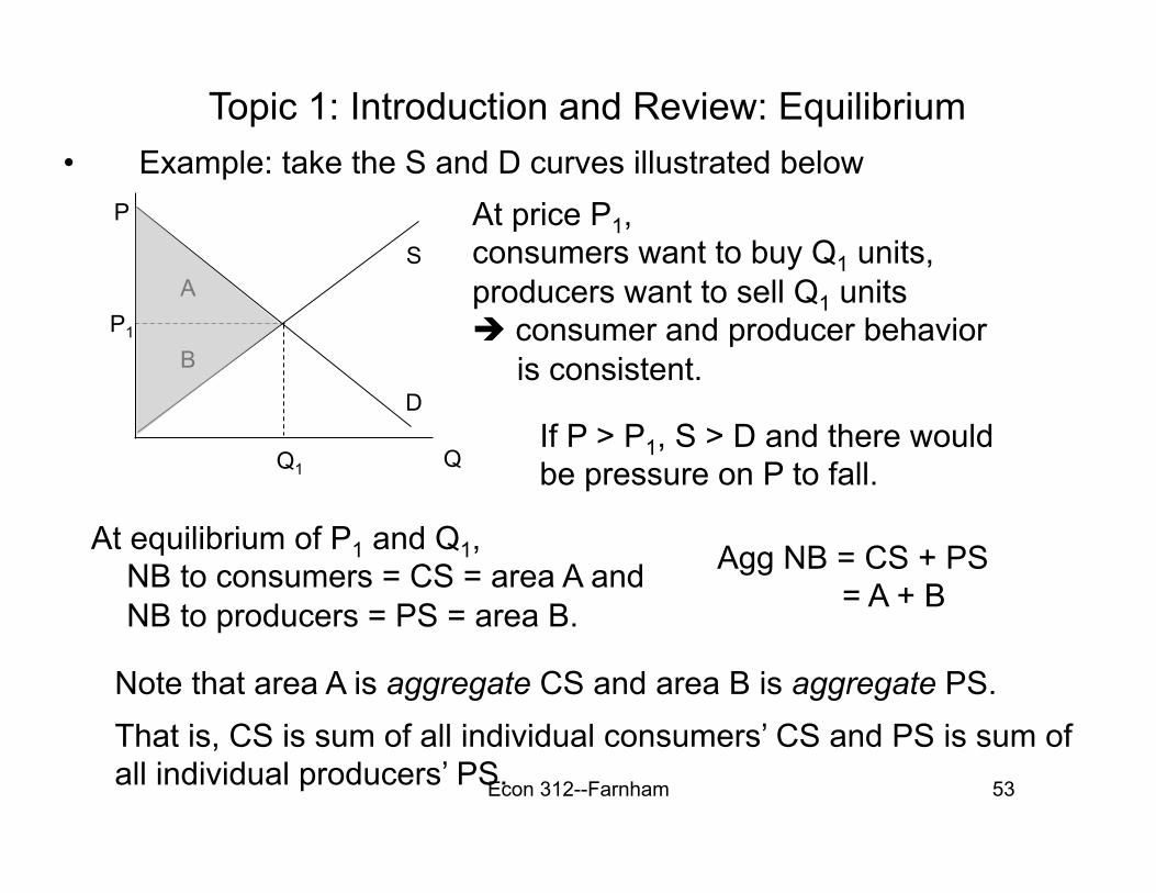
Topic 1: Introduction and Review: Equilibrium • Example: take the S and D curves illustrated below
Q1
P1
P
Q
S
D
At price P1, consumers want to buy Q1 units, producers want to sell Q1 units consumer and producer behavior is consistent.
If P > P1, S > D and there would be pressure on P to fall.
At equilibrium of P1 and Q1, NB to consumers = CS = area A and NB to producers = PS = area B.
Agg NB = CS + PS = A + B
A
B
Note that area A is aggregate CS and area B is aggregate PS. That is, CS is sum of all individual consumers’ CS and PS is sum of all individual producers’ PS.

Topic 1: Introduction and Review: Equilibrium • One very important thing to note: aggregate NB always the same
if Q the same, no matter what happens to P.
• Another way of saying this is that aggregate NB function only of total Q, while the distribution of NB depends on P.
Q1
P1
P
Q
S
D
Example: here equilibrium would be P1, Q1. But, if government imposes a quota at Q2, new equilibrium would be at P2, Q2 where: CS = A PS = B + C + D
But now suppose that (instead of quota), government instead says P cannot rise above P3 (“price ceiling”). Equilibrium still Q2 but with different P. Now we have: CS = A + B + C PS = D
Agg NB = CS + PS = A + B + C + D
Q2
P2 A B C
P3 D
Agg NB = A + B + C + D Same in total, distribution different.
Econ 312--Farnham 55
Topic 1: Introduction and Review Summary:
• We have seen that (absent quotas, price ceilings etc): – Consumers choose Q such that P = MB
• i.e., choose to consume where P cuts D curve. • NB to consumers = CS.
– Producers choose Q such that P = MC • i.e. choose to produce where P line cuts S curve. • NB to producers = PS.
– Producer and consumer decisions are such that S=D • Aggregate NB = sum of individual NB • Sum of individual NB = CS + PS (if consumers and
producers are the the only agents affected by the market).
• Note that these are positive questions - describing the way in which markets DO work.
• Can also ask corresponding normative questions.
Econ 312--Farnham 56
Topic 1: Introduction and Review • Normative questions of interest are:
1. What quantity of goods should be produced? • We know that in equilibrium Q is where S=D. • Under what circumstances is this the “right” Q in total (the one
that maximizes NB)?
2. Which firms should produce these goods? • We know that in equilibrium each firm produces until P=MC. • Under what circumstances is the the “right” Q for each firm (the
one that minimizes aggregate production costs)?
3. Which consumers should get to consume these goods? • We know that in equilibrium each consumer chooses Q such
that P=MB. • Under what circumstances is the the “right” Q for each
consumer (the one that maximizes aggregate benefits from consumption)?
Econ 312--Farnham 57
Topic 1: Introduction and Review • We will focus primarily on question (1). The efficient allocation will
occur (in all cases discussed in this course) where MC=MB. – Try to understand the intuition for this:
• If MC>MB, this tells us the last little bit produced cost more to produce that it gave to consumers in added benefit. Society would be better off with less of the good (Q should fall).
• If MC<MB, this tells us the last little bit produced cost less to produce that it gave to consumers in added benefit. This suggest that increasing output would raise overall well-being in society (Q should rise).
• If MC=MB, this tells us the last little bit produced cost exactly the same amount to produce as it gave consumers in added benefit. This tells us this unit made society no better off than it was before (nor any worse off). This is the efficient point.
– Note that MC=MB in the equilibrium diagram 4 slides back. In a well-functioning market, MC=MB at equilibrium so that the equilibrium is efficient. However, this does not always have to be the case!
• When market failure occurs (due to something like the presence of an externality or due to monopolistic control of an industry), it may not be the case that MC=MB at equilibrium
• In such a case, the equilibrium quantity may be different from the efficient quantity.


