21
Economics 5550 Statistical Tools
| Date post: | 21-Dec-2015 |
| Category: |
Documents |
| View: | 214 times |
| Download: | 0 times |

Economics 5550
Statistical Tools
Statistics and Hypotheses
• If you are following the health care system, you see a lot of discussion. Let's consider health care costs. Most simply:
• How fast are they rising?
• Are ours higher than Canada's; if so how much?
• Do HMO's reduce costs; if so, how much?
• Are patients in managed care settings sicker, healthier; if so how much?

Most of the time, such assertions are made with certainty. Yet, they are almost certainly not certain. These involve testing hypotheses.
Many of you have had some passing experience with experimental laboratory work. Most often the work is a demonstration, rather than an experiment (i.e. mix up these 2 chemicals and you'll blow up the lab).
Let's see what we have in mind with empirical work.
Statistics and Hypotheses
Why?Economists look at statements that while plausible, merit
validation. Suppose for example that you are looking at a public health intervention that would seek to reduce cholesterol in the population. One useful question for targeting the intervention is who has a higher cholesterol level, men or women?
Why is this important?<A.1> It could turn out that one group is at risk, and another
group isn't.
<A.2> You just want to know.
How do we formulate hypotheses?
The style is to use the "null" hypothesis; then contrast it to the "alternative" hypothesis.
Let's look at a sample of Wayne State college sophomores. We'll discuss this in more detail as we go along. We customarily refer to the null hypothesis as H0, and the alternative hypothesis as H1. So,
H0 : cm = cw.
H1 : cm cw.
H0 : cm = cw.
H1 : cm cw.
So, if cm seems to be about the same as cw, we'll accept the null hypothesis. If it seems to be different, we'll reject the null hypothesis. This type of hypothesis is called a "simple hypothesis."
Simple Hypotheses
Composite Hypotheses
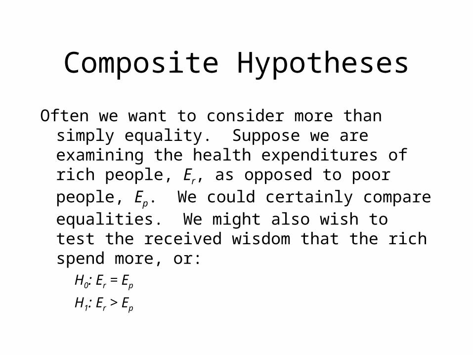
Often we want to consider more than simply equality. Suppose we are examining the health expenditures of rich people, Er, as opposed to poor people, Ep. We could certainly compare equalities. We might also wish to test the received wisdom that the rich spend more, or:
H0: Er = Ep
H1: Er > Ep
Composite Hypotheses
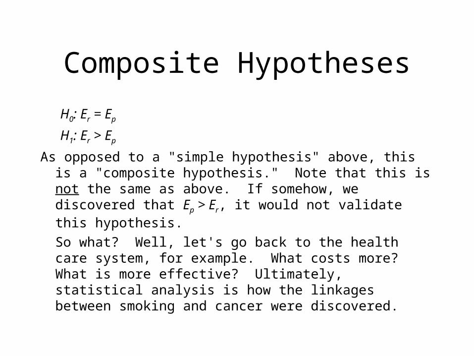
H0: Er = Ep
H1: Er > Ep
As opposed to a "simple hypothesis" above, this is a "composite hypothesis." Note that this is not the same as above. If somehow, we discovered that Ep > Er, it would not validate this hypothesis.
So what? Well, let's go back to the health care system, for example. What costs more? What is more effective? Ultimately, statistical analysis is how the linkages between smoking and cancer were discovered.
So, how do we test hypotheses?
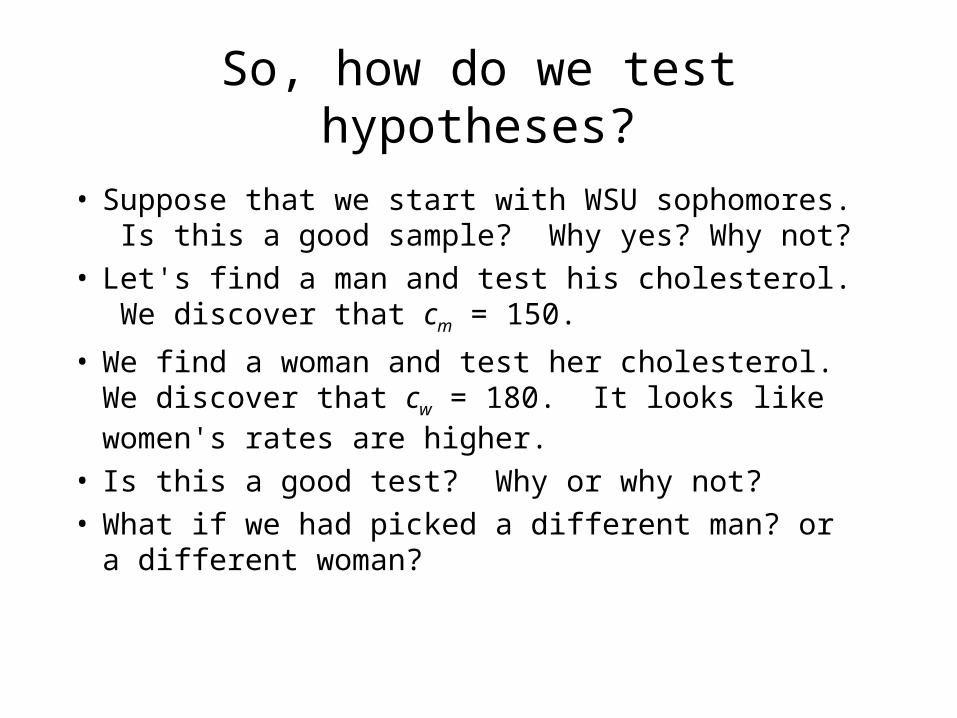
• Suppose that we start with WSU sophomores. Is this a good sample? Why yes? Why not?
• Let's find a man and test his cholesterol. We discover that cm = 150.
• We find a woman and test her cholesterol. We discover that cw = 180. It looks like women's rates are higher.
• Is this a good test? Why or why not? • What if we had picked a different man? or a different
woman?
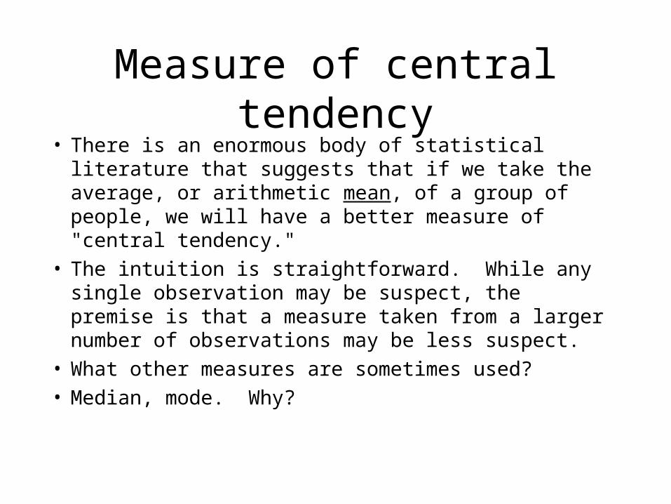
Measure of central tendency• There is an enormous body of statistical literature that
suggests that if we take the average, or arithmetic mean, of a group of people, we will have a better measure of "central tendency."
• The intuition is straightforward. While any single observation may be suspect, the premise is that a measure taken from a larger number of observations may be less suspect.
• What other measures are sometimes used?
• Median, mode. Why?
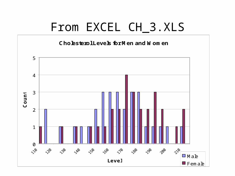
From EXCEL CH_3.XLSCholesterol Levels for Men and Women
0
1
2
3
4
5
Level
Co
un
t
Male
Female
Hypothesis testing
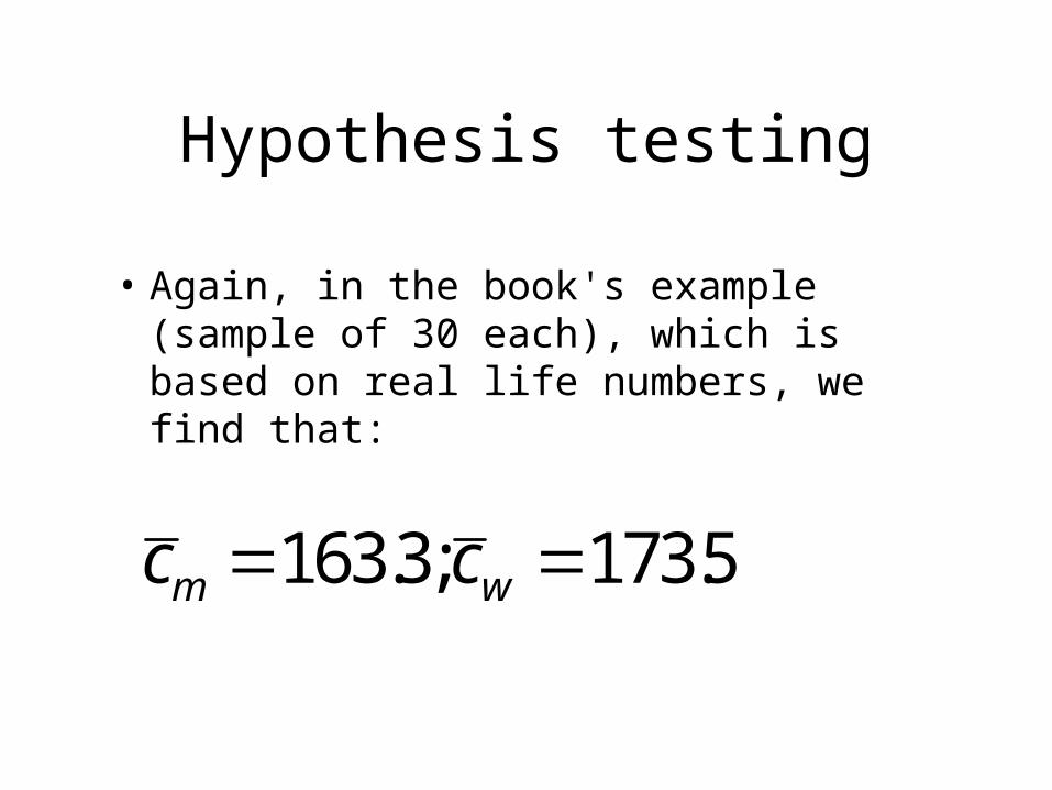
• Again, in the book's example (sample of 30 each), which is based on real life numbers, we find that:
c cm w 1633 1735. ; .
Hypothesis testing
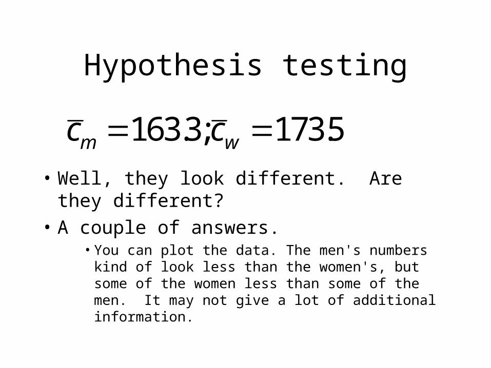
• Well, they look different. Are they different?• A couple of answers.
• You can plot the data. The men's numbers kind of look less than the women's, but some of the women less than some of the men. It may not give a lot of additional information.
c cm w 1633 1735. ; .
Testing Differences
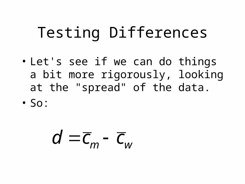
• Let's see if we can do things a bit more rigorously, looking at the "spread" of the data.
• So:
d c cm w

Testing Differences
• We'd like to determine whether the difference d could have been generated randomly; that is, what is the possibility that in truth cw = cm, and somehow we just managed to find 2 samples that generated these separate means?
• We want to compare the difference to the spread. If the difference is large (relative to the spread), it would seem to be unlikely that it was caused at random. If it is small, it might have been caused at random.
d c cm w

Testing Differences
• A useful way, and by far the most frequent way, that we calculate the "spread" is to subtract each value from the mean, square the term, add the squared terms, and divide by the number of observations.
Vwx x x x x x
Nn
( ) ( ) ...( )12
22 2
Testing Differences
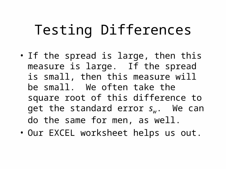
• If the spread is large, then this measure is large. If the spread is small, then this measure will be small. We often take the square root of this difference to get the standard error sw. We can do the same for men, as well.
• Our EXCEL worksheet helps us out.
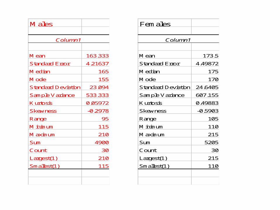
Males
Column1
Mean 163.333
Standard Error 4.21637
Median 165
Mode 155
Standard Deviation 23.094
Sample Variance 533.333
Kurtosis 0.05972
Skewness -0.2978
Range 95
Minimum 115
Maximum 210
Sum 4900
Count 30
Largest(1) 210
Smallest(1) 115
Females
Column1
Mean 173.5
Standard Error 4.49872
Median 175
Mode 170
Standard Deviation 24.6405
Sample Variance 607.155
Kurtosis 0.49883
Skewness -0.5903
Range 105
Minimum 110
Maximum 215
Sum 5205
Count 30
Largest(1) 215
Smallest(1) 110
Testing Differences
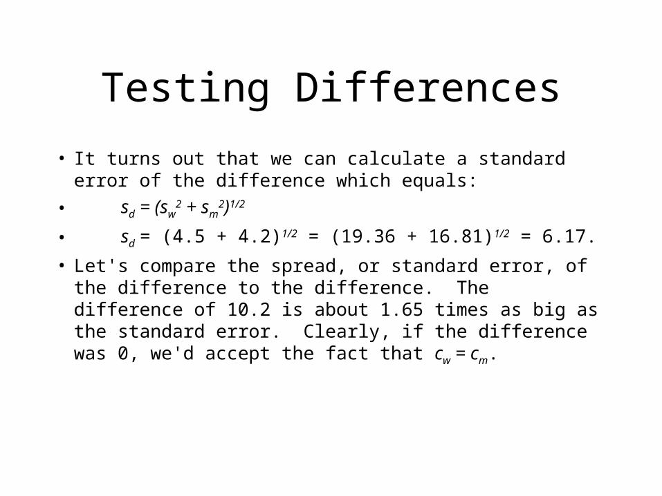
• It turns out that we can calculate a standard error of the difference which equals:
• sd = (sw2 + sm
2)1/2
• sd = (4.5 + 4.2)1/2 = (19.36 + 16.81)1/2 = 6.17.
• Let's compare the spread, or standard error, of the difference to the difference. The difference of 10.2 is about 1.65 times as big as the standard error. Clearly, if the difference was 0, we'd accept the fact that cw = cm.
Testing Differences
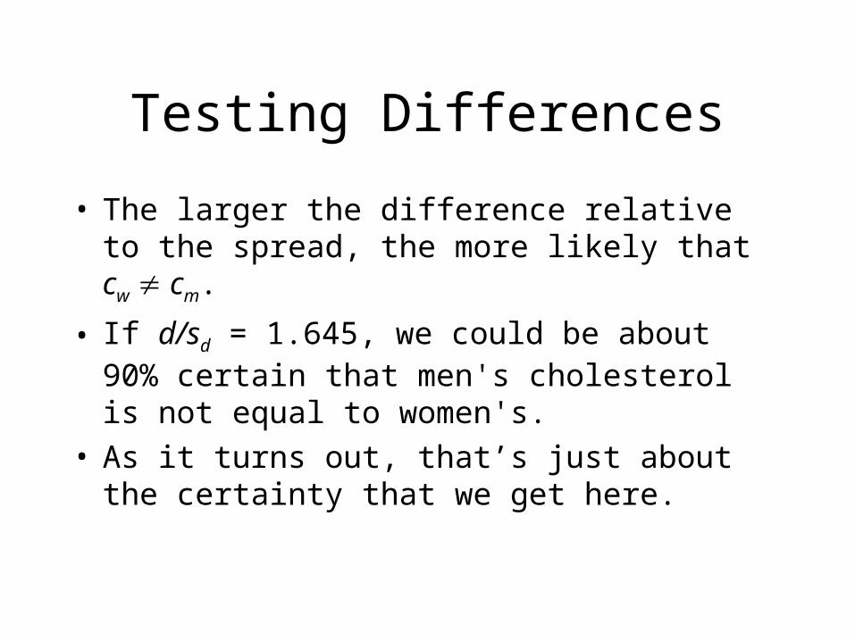
• The larger the difference relative to the spread, the more likely that cw cm.
• If d/sd = 1.645, we could be about 90% certain that men's cholesterol is not equal to women's.
• As it turns out, that’s just about the certainty that we get here.
Key points for hypothesis testing:
State hypotheses clearly
Choose suitable sample
Calculate appropriate measures of central tendency and dispersion
Draw appropriate inferences


