ECONOMICS 8346, Fall 2013 Bent E. Sørensen Introduction to Panel Data A panel data set (or just a panel) is a set of data (y it ,x it )(i =1,...,N ; t = 1,...T ) with two indices. Assume that you want to estimate the model y it = X it β + ² it where var(² it )= σ 2 ,y it is a scalar, and x it is 1 × k vector containing k regressors. There are three well-known (and inexpensive) textbooks on panel data (all quite good and likely available in paperback): Hsiao: Analysis of Panel Data, Cambridge University Press, 1986). Baltagi: Econometric Analysis of Panel Data, Wiley, 1995. Arellano: Panel Data Econometrics, Oxford University Press, 1995. The Hsiao book is a little dated by now and more focussed on micro-applications, but it is still good to read. Arellano’s book is probably the most comprehensive and it is very well written. The only draw-back is that is it covers more ground that you would want if you are new to field. Baltagi’s book is also good. This note here is intended to get you started, see also the much-used first-year graduate textbook by Greene, Ch. 14. (By the way: Arellano’s book has an appendix on GMM that looks quite accessible.) You should check for new versions and I recommend checking Arellano’s web-page (http://www.cemfi.es/ arellano/) for recent work if you need to go deeper. Examples 1
Transcript
ECONOMICS 8346, Fall 2013
Bent E. Sørensen
Introduction to Panel Data
A panel data set (or just a panel) is a set of data (yit, xit) (i = 1, . . . , N ; t =
1, . . . T ) with two indices.
Assume that you want to estimate the model
yit = Xitβ + εit
where var(εit) = σ2, yit is a scalar, and xit is 1× k vector containing k regressors.
There are three well-known (and inexpensive) textbooks on panel data (all quite good
and likely available in paperback):
Hsiao: Analysis of Panel Data, Cambridge University Press, 1986).
Baltagi: Econometric Analysis of Panel Data, Wiley, 1995.
Arellano: Panel Data Econometrics, Oxford University Press, 1995.
The Hsiao book is a little dated by now and more focussed on micro-applications,
but it is still good to read. Arellano’s book is probably the most comprehensive and
it is very well written. The only draw-back is that is it covers more ground that you
would want if you are new to field. Baltagi’s book is also good. This note here is
intended to get you started, see also the much-used first-year graduate textbook by
Greene, Ch. 14. (By the way: Arellano’s book has an appendix on GMM that looks
quite accessible.) You should check for new versions and I recommend checking Arellano’s
web-page (http://www.cemfi.es/ arellano/) for recent work if you need to go deeper.
Examples
1
1. Assume you have quarterly observations of ys, xs for the period (say) 1960.1 →1989.4. If you want to stress that quarters are different from years, you can write,
e.g., the ys data as
yit where i is year and t is quarter
and you may feel like storing the y-data in a matrix
Y = [yit] =
y1960,1 y1960,2 . . . y1960,4...
...y1989,1 . . . . . . y1989,4
Usually one doesn’t write the model with quarterly data like this. Example 1
demonstrates that whether you write ys, s = 1, . . . , 160 (NT ) or yit (i =
1, . . . , 40 (N); t = 1, . . . , 4 (T )) is just a convention. Albeit often a practical
convention which we use if we want to work with models that display different
features for the t-index than for the i index.
2. Very typical micro example. Assume that you observe (say) wages wit and experi-
ence (and age, education,...) Xit for a sample of individuals i = 1, . . . , N over
time t = 1, . . . , T.
This is the type of panel that most people think of when you say “panel data.”
For this type of data you usually have N large (thousands) and T small (often
2 or 3 and 30–40 at the most).
A much utilized data set in the US is the PSID a panel which have been following
a sample of 4000 + US families since 1968.
Close to 1000 articles have been published using the PSID.
A lot of theoretical econometric work on panel data is relevant for small T, large N
and until very recently “panel data” was considered a microeconometrics subfield.
2
(“Small” T and “large” N means that one relies on asymptotic theory derived
keeping T fixed and letting N go to infinity.) For this class, however, we are more
interested in macro-panels with a rather small N dimension (by the standards of,
say, labor-economists). The econometric issues are somewhat different for such
panels.
3. A typical macro example is a “consumption function” (simplified a bit)
and since third column is XUK × (first column) + XUS × (second column) the
matrix is singular = perfect multicolinearity.
Dummy variables for each time period (“time-fixed effects”) are treated the same way
and the inclusion of both state- and time-fixed effects is easily handled by removing the
time-specific and the state-specific averages sequentially.
In Asdrubali, Sørensen, and Yosha (1996), the inclusion of time-fixed effects is cru-
cial for the interpretation of the regressions as risk sharing estimations. As argued, for
example by Cochrane (1991), there are reasons to believe that it is more robust to include
a constant in a cross-sectional risk sharing regression than it is to control for aggregate
consumption. In this connection, if is important to realize that a panel regression with
8
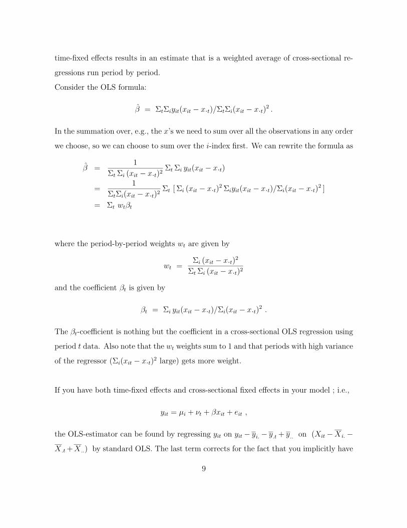
time-fixed effects results in an estimate that is a weighted average of cross-sectional re-
gressions run period by period.
Consider the OLS formula:
β = ΣtΣiyit(xit − x.t)/ΣtΣi(xit − x.t)2 .
In the summation over, e.g., the x’s we need to sum over all the observations in any order
we choose, so we can choose to sum over the i-index first. We can rewrite the formula as
β =1
Σt Σi (xit − x.t)2Σt Σi yit(xit − x.t)
=1
ΣtΣi(xit − x.t)2Σt [ Σi (xit − x.t)
2 Σiyit(xit − x.t)/Σi(xit − x.t)2 ]
= Σt wtβt
where the period-by-period weights wt are given by
wt =Σi (xit − x.t)
2
Σt Σi (xit − x.t)2
and the coefficient βt is given by
βt = Σi yit(xit − x.t)/Σi(xit − x.t)2 .
The βt-coefficient is nothing but the coefficient in a cross-sectional OLS regression using
period t data. Also note that the wt weights sum to 1 and that periods with high variance
of the regressor (Σi(xit − x.t)2 large) gets more weight.
If you have both time-fixed effects and cross-sectional fixed effects in your model ; i.e.,
yit = µi + νt + βxit + eit ,
the OLS-estimator can be found by regressing yit on yit− yi.− y.t + y.. on (Xit−X i.−X .t +X ..) by standard OLS. The last term corrects for the fact that you implicitly have
9
subtracted the constant twice and if you don’t allow for a constant in this OLS regression
you have to correct for that.
If you subtract the time and cross-sectional means and then have, say, Stata, run the
OLS regression, you need to adjust the standard errors, because you have used N +T −1
degrees for freedom before sending the data to the regression. Y
If you have missing data, you need to make sure that all means are calculated on the
same data and those are the same used in the regression (so if there one (i,t) pair where,
say, y, is missing that has to be dropped before you calculate means for regressors).
Modeling the variance
In panel data sets it is often reasonable to expect that the variance of the error term
is different for each state (person, ...) or time period. For example, considering the
value of output of states or countries, there is no doubt that oil-states display higher
variance than other states. Or maybe consumption patterns in neighboring states are
more similar to each other than they are to those of more distant states. In principle the
econometrics is simple. If the NT ×NT matrix of residuals is Ω then the GLS estimator
of β is β = (X ′ Ω−1X)−1X ′ Ω−1y. The feasible GLS estimator that one usually need to
use is a 2-step estimator where one first performs OLS and then estimates Ω and plugs
the estimated Ω into the GLS formula.
Occasionally one may want to estimate β by OLS, even if the error covariance matrix
is Ω. In this case one still needs to estimate Ω since the variance of the OLS estimator
then is given by (X ′X)−1 X ′ Ω X (X ′X)−1. In Asdrubali, Sørensen, and Yosha (1996) we
estimated a complicated Ω matrix, but since the estimated Ω was likely to be imprecise,
we found it unattractive to invert it and therefore used OLS with “GLS errors.” (This is
sometimes called a “generalized linear model.”) In the article “Consumption and Aggre-
10
gate Constraints: Evidence from U.S. States and Canadian Provinces” by Ostergaard,
Sørensen, and Yosha (JPE 2002) we did invert the Ω matrix at the prompting of a ref-
eree; my software/memory couldn’t handle the size of the matrix so I spent a long time
figuring out how to do it by splitting it up in smaller sub-matrices—you don’t want to
know the details but I have the program if you ever need it.
For simpler models, when the dimension of Ω is too large to keep in memory, one can
often transform the data to be independent. (Formally, this means calculate y = Ω−1/2y
and X = Ω−1/2X and then run OLS on X and y.)
As the simplest example, consider the model
yit = Xitβ + εit
where var(εit) = σ2i . (Each “state” has a different variance.) The model may or may not
contain fixed effects, that doesn’t affect the following. Such a model is easily estimated
by 2-step estimation of Maximum Likelihood (ML). The variance matrix takes the form
Ω =
σ21 · · · 0 · · · 0 · · · 0
.... . .
......
.... . .
...0 · · · σ2
1 · · · 0 · · · 0...
.... . .
......
0 · · · 0 · · · σ2N · · · 0
.... . .
......
.... . .
...0 · · · 0 · · · 0 · · · σ2
N
.
(Assuming the data are stacked with state 1’s data first, then state 2, etc.) The 2-step
(feasible GLS) estimator’s first step is to estimate the model by OLS, and then estimate
the Ω matrix from the residuals and transform the data to have diagonal covariance
matrix. In practice, estimate σ2i =
∑Tt=1 e2
it, where the (eit) matrix is the residuals from
an OLS regression; then transform the data to yit = yit/σi and xit = xit/σi, and run OLS
on the transformed data. (Iterating the process will give the ML estimator.) This is, of
11
course, a standard correction for heteroskedasticity. In Asdrubali, Sørensen, and Yosha
(1996), it was found that correcting for state-specific heteroskedasticity had some effect
on the estimates.
One may also want to correct for time-specific heteroskedasticity (similar) or both state-
and time-specific heteroskedasticity. In the latter case, the variance matrix becomes
more complicated, but again one simply adjust the data by the estimated time- and
state-specific standard deviations.
If, say, the T dimension is low, one may want to allow for a totally general pattern
of time- (auto-) correlation. Assume now that the data are stacked as above, the vari-
ance matrix then takes the form
Ω =
Γ . . . 0...
. . ....
0 . . . Γ
.
The Ω matrix has the form Ω = I ⊗ Γ, where “⊗” is the so-called Kronecker product,
which signifies that each element in the first matrix gets multiplied by the second ma-
trix. (Here I is an N×N identity matrix and Σ is the variance-covariance matrix for the
T observations for state i, assumed to be the same for each i.) The Γ-matrix contains
T ∗(T +1)/2 parameters and cannot be estimated from a single time series (therefore the
whole topics of time series analysis is mainly about constructing parameter-parsimonious
models for Γ), but it can be estimated from a panel with N > T . The Γ matrix is easily
estimated after a first step estimation as Γst = 1N
ΣNi=1eiseit ; s = 1, ..., T , t = 1, ..., T .
One can fairly easily show that that (I⊗Γ)−1 = I⊗Γ−1 and one can then use the standard
GLS estimator: β = (X ′ Ω−1 X)−1(X ′ Ω−1 y). As usual, the problem is how to invert
the NT−matrix Ω, but if one defines Xi = xit ; t = 1, ..., T and yi = yit ; t = 1, ..., T
12
then it is easy to realize (using partitioned matrices) that
X ′ Ω−1 X = ΣNi=1 X ′
i Γ−1 Xi ,
and similarly for X ′ Ω−1 y . So only matrices of dimension T × T need to be inverted.
For the 2-step estimator the calculation will, of course, involve Γ rather than Γ.
In Asdrubali, Sørensen, and Yosha (1996) we postulated a simple AR(1) model for the
time series dependence of the residuals. (In our experience with estimating risk sharing
panel data models on U.S. states and OECD countries, it has little effect on the esti-
mates to control for auto-correlation.) For cross-correlation between states we estimated
a 50× 50 unrestricted variance-covariance matrix (likely to imprecisely estimated). The
problem with modeling spatial correlations is that there is not obvious parsimonious
model. Some suggestions is to let the variance decline with distance (analogously to
the AR(1) model, but is there any really reason to believe that, e.g., Massachusetts is
more similar to a nearby rural state like Maine, than it is to another financial center like
Chicago? It is hard to know, and hard to test for.
Random Effect Models
The most commonly used variance model is the “random effect model.” The mate-
rial is here as a (rigorous) introduction to the topic. The textbooks mentioned contain
much more material on random effect models. One reason to cover it here is that it
gives a nice example of the way one has to analytically figure out how to invert large
covariance matrices in panels.
The (one-way) random-effect model takes the form
(∗) yit = Xitβ + µi + εit ; i = 1, . . . , N , t = 1, . . . , T ,
13
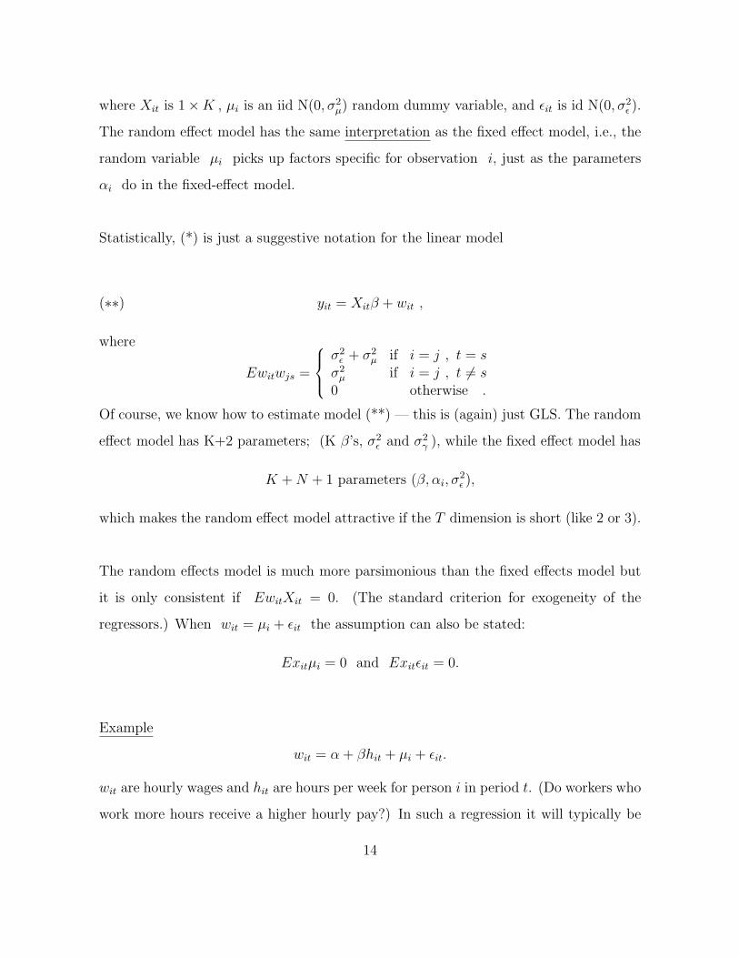
where Xit is 1×K , µi is an iid N(0, σ2µ) random dummy variable, and εit is id N(0, σ2
ε ).
The random effect model has the same interpretation as the fixed effect model, i.e., the
random variable µi picks up factors specific for observation i, just as the parameters
αi do in the fixed-effect model.
Statistically, (*) is just a suggestive notation for the linear model
(∗∗) yit = Xitβ + wit ,
where
Ewitwjs =
σ2ε + σ2
µ if i = j , t = sσ2
µ if i = j , t 6= s0 otherwise .
Of course, we know how to estimate model (**) — this is (again) just GLS. The random
effect model has K+2 parameters; (K β’s, σ2ε and σ2
γ ), while the fixed effect model has
K + N + 1 parameters (β, αi, σ2ε ),
which makes the random effect model attractive if the T dimension is short (like 2 or 3).
The random effects model is much more parsimonious than the fixed effects model but
it is only consistent if EwitXit = 0. (The standard criterion for exogeneity of the
regressors.) When wit = µi + εit the assumption can also be stated:
Exitµi = 0 and Exitεit = 0.
Example
wit = α + βhit + µi + εit.
wit are hourly wages and hit are hours per week for person i in period t. (Do workers who
work more hours receive a higher hourly pay?) In such a regression it will typically be
14
hard to defend exogeneity. But now assume that person i (Mr. Smith) for other reasons
have a relatively high hourly wage (µSmith > 0). It is then likely that the high wage
induces Mr. Smith to work longer (or shorter) hours. So again the crucial assumption
Eµixit = 0 is unlikely to hold.
In general, it is often a very strong assumption (meaning that is likely not true) to impose
Eµixit = 0.
It is usually assumed that µi and εit are normally distributed. This could also be
wrong – e.g., if µi ‘picks up’ things like wealth, it would be more likely to be log-normal.
(If the distribution is known, one may figure out how to solve the problem, but usually
one has little to go by, when selecting a model for µi.)
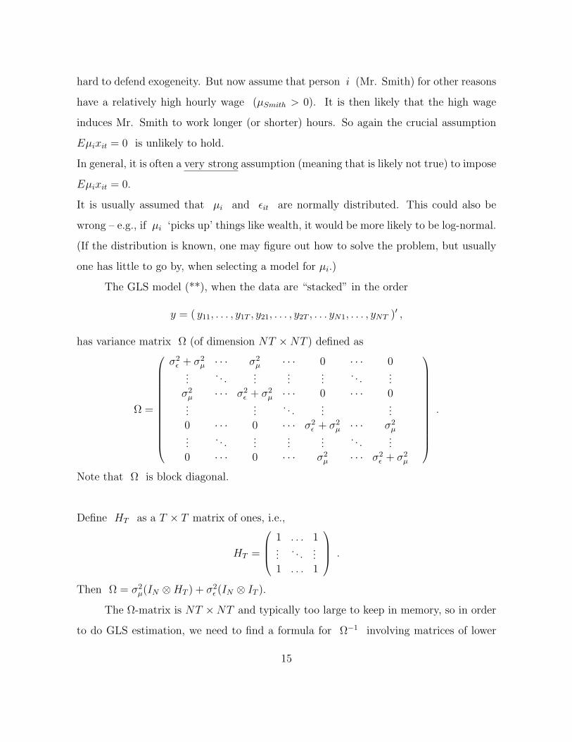
The GLS model (**), when the data are “stacked” in the order
has variance matrix Ω (of dimension NT ×NT ) defined as
Ω =
σ2ε + σ2
µ · · · σ2µ · · · 0 · · · 0
.... . .
......
.... . .
...σ2
µ · · · σ2ε + σ2
µ · · · 0 · · · 0...
.... . .
......
0 · · · 0 · · · σ2ε + σ2
µ · · · σ2µ
.... . .
......
.... . .
...0 · · · 0 · · · σ2
µ · · · σ2ε + σ2
µ
.
Note that Ω is block diagonal.
Define HT as a T × T matrix of ones, i.e.,
HT =
1 . . . 1...
. . ....
1 . . . 1
.
Then Ω = σ2µ(IN ⊗HT ) + σ2
ε (IN ⊗ IT ).
The Ω-matrix is NT ×NT and typically too large to keep in memory, so in order
to do GLS estimation, we need to find a formula for Ω−1 involving matrices of lower
15
dimensions.
This can be done cleverly in the following fashion: (the notation here follows Balt-
agi’s book.)
Define the T × T matrix
JT =
1T
. . . 1T
.... . .
...1T
. . . 1T
and
ET = IT − JT =
(1− 1T) . . . − 1
T...
...− 1
T. . . (1− 1
T)
Now both JT and ET are idempotent, e.g.,
[JT JT ]ij = [∑T
t=11
T 2 ]ij = [T 1T 2 ]ij
= [ 1T]ij = [JT ]ij .
Also,
ET JT = (IT − JT )JT = 0
so ET and JT are orthogonal.
Define P = IN ⊗ JT and Q = IN ⊗ ET then P, Q are also idempotent and or-
thogonal.
NowΩ = σ2
µ(IN ⊗HT ) + σ2ε (IN ⊗ IT )
= Tσ2µ(IN ⊗ JT ) + σ2
ε (IN ⊗ ET ) + σ2ε (IN ⊗ JT )
= (Tσ2µ + σ2
ε )(IN ⊗ JT ) + σ2ε (IN ⊗ ET )
= (Tσ2µ + σ2
ε )P + σ2ε Q
16
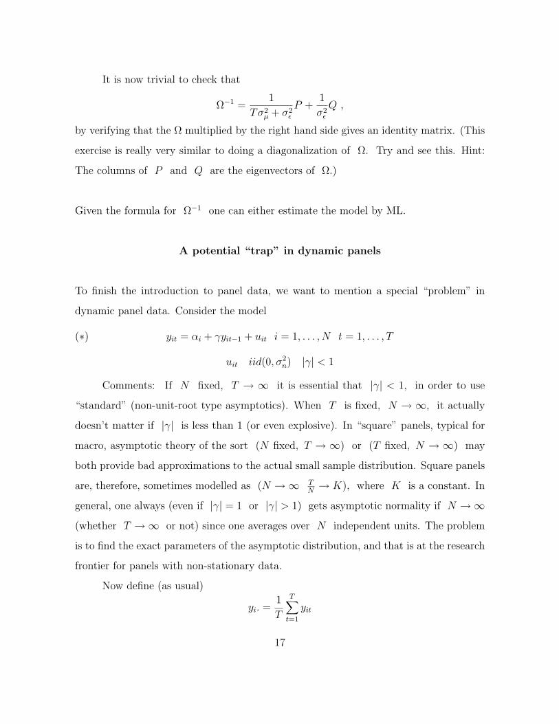
It is now trivial to check that
Ω−1 =1
Tσ2µ + σ2
ε
P +1
σ2ε
Q ,
by verifying that the Ω multiplied by the right hand side gives an identity matrix. (This
exercise is really very similar to doing a diagonalization of Ω. Try and see this. Hint:
The columns of P and Q are the eigenvectors of Ω.)
Given the formula for Ω−1 one can either estimate the model by ML.
A potential “trap” in dynamic panels
To finish the introduction to panel data, we want to mention a special “problem” in
dynamic panel data. Consider the model
(∗) yit = αi + γyit−1 + uit i = 1, . . . , N t = 1, . . . , T
uit iid(0, σ2n) |γ| < 1
Comments: If N fixed, T → ∞ it is essential that |γ| < 1, in order to use
“standard” (non-unit-root type asymptotics). When T is fixed, N → ∞, it actually
doesn’t matter if |γ| is less than 1 (or even explosive). In “square” panels, typical for
macro, asymptotic theory of the sort (N fixed, T → ∞) or (T fixed, N → ∞) may
both provide bad approximations to the actual small sample distribution. Square panels
are, therefore, sometimes modelled as (N →∞ TN→ K), where K is a constant. In
general, one always (even if |γ| = 1 or |γ| > 1) gets asymptotic normality if N →∞(whether T →∞ or not) since one averages over N independent units. The problem
is to find the exact parameters of the asymptotic distribution, and that is at the research
frontier for panels with non-stationary data.
Now define (as usual)
yi. =1
T
T∑
t=1
yit
17
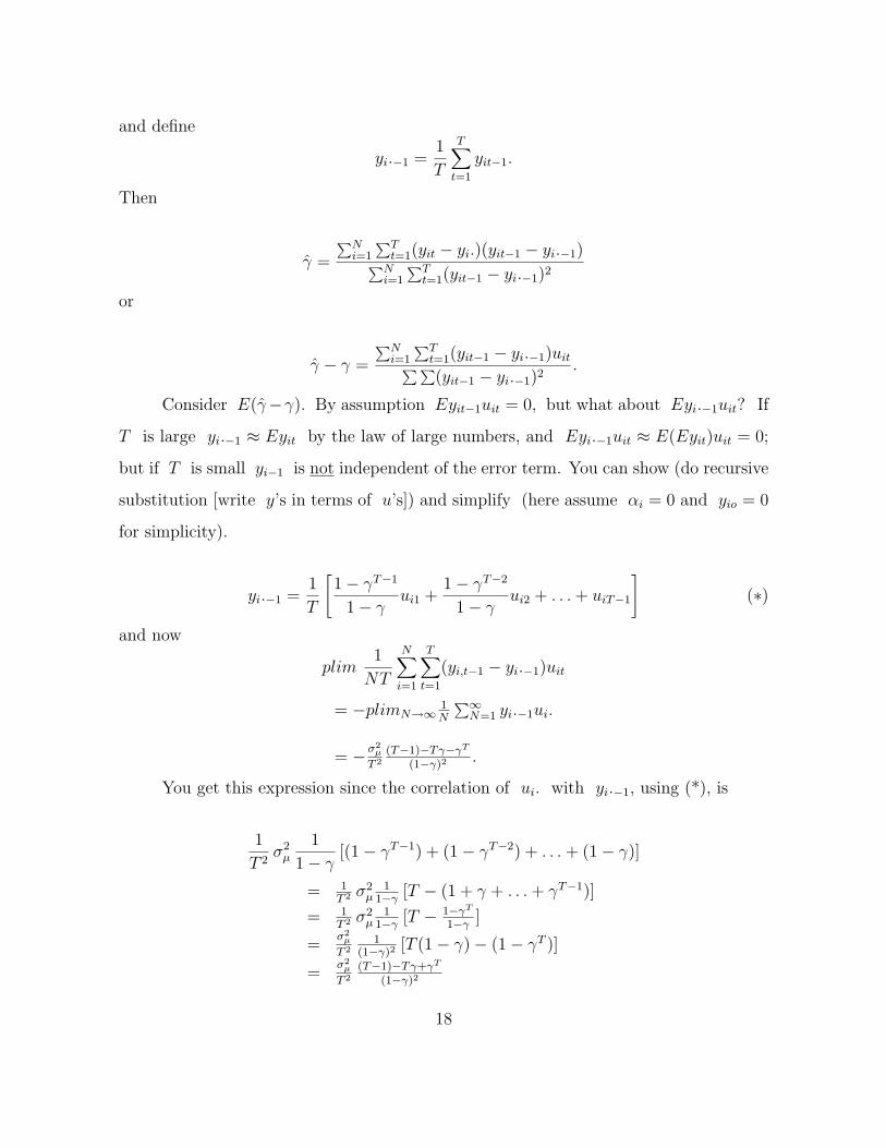
and define
yi.−1 =1
T
T∑
t=1
yit−1.
Then
γ =
∑Ni=1
∑Tt=1(yit − yi.)(yit−1 − yi.−1)∑N
i=1
∑Tt=1(yit−1 − yi.−1)2
or
γ − γ =
∑Ni=1
∑Tt=1(yit−1 − yi.−1)uit∑ ∑(yit−1 − yi.−1)2
.
Consider E(γ−γ). By assumption Eyit−1uit = 0, but what about Eyi.−1uit? If
T is large yi.−1 ≈ Eyit by the law of large numbers, and Eyi.−1uit ≈ E(Eyit)uit = 0;
but if T is small yi−1 is not independent of the error term. You can show (do recursive
substitution [write y’s in terms of u’s]) and simplify (here assume αi = 0 and yio = 0
for simplicity).
yi.−1 =1
T
[1− γT−1
1− γui1 +
1− γT−2
1− γui2 + . . . + uiT−1
](∗)
and now
plim1
NT
N∑
i=1
T∑
t=1
(yi,t−1 − yi.−1)uit
= −plimN→∞ 1N
∑∞N=1 yi.−1ui.
= −σ2µ
T 2(T−1)−Tγ−γT
(1−γ)2.
You get this expression since the correlation of ui. with yi.−1, using (*), is
1
T 2σ2
µ
1
1− γ[(1− γT−1) + (1− γT−2) + . . . + (1− γ)]
= 1T 2 σ2
µ1
1−γ[T − (1 + γ + . . . + γT−1)]
= 1T 2 σ2
µ1
1−γ[T − 1−γT
1−γ]
=σ2
µ
T 21
(1−γ)2[T (1− γ)− (1− γT )]
=σ2
µ
T 2(T−1)−Tγ+γT
(1−γ)2
18
Similarly, one can show that
plim1
NT
∑ ∑(yit−1 − yi.−1)
2
=σ2
µ
1− γ21− 1
T− 2γ
(1− γ)2· (T − 1)− Tγ + γT
T 2
So, in total
plimN→∞(γ − γ) = −(1 + γ)
T − 1(1− 1
T
1− γT
1− γ)× 1− 2γ
(1− γ)(T − 1)
[1− 1− γT
T (1− γ)
]−1.
I haven’t done the derivation of the last two equations (they are taken from Hsiao’s
book), you may want to do the exercise of deriving one of them on your own.
If T = 2 (for example), this is a huge bias = −1 + (1− 12) = −.5 (when γ = 0).
Notice, that the bias does not go away if γ = 0 (the bias remains as long as one attempts
to estimate the γ parameters). Typical suggested solution:
Difference to get the model
∆yit = γ∆yit−1 −∆uit
(which no longer contains fixed effects) AND
(a) estimate γ by IV estimation, using yit−2 as instrument. OR
(b) estimate γ by IV estimation, using yi0 as instrument for period 2, yi0, yi1 for
period 3, yi0, yi1, yi2 for period 4, etc.
If the original equation has iid errors, the differenced equation has a unit root in the
AR-process of the error-term, which necessitates the use of the twice lagged variables
as instruments. One drawback of (a) is that the lagged variable may or may not be a
good instrument—if γ is small, it is a lousy instrument. Using all lagged variables as
in (b) is asymptotically efficient—I don’t have practical experience with this estimator
(although, if T is large you are using a large amount of instruments and I would tend to
19
wonder about the quality of the estimated standard errors). If you use this type of panel
regressions in serious work you should study the issue more, starting with Arellano’s
book.
Panel Unit Roots and Panel Co-Integration (just a few comments on the
issues)
These are areas with a lot of current active research. There is a survey article by Baner-
jee in the Oxford Bulletin of Economics and Statistics (1999) and you may also want to
look at Chapter 7 of the Textbook “Applied Time Series Modelling and Forecasting” by
Harris and Sollis (Wiley 2003). Peter Pedroni has a lot of articles on these issues and a
book in process, check his WEB-page.
Note that if T is small you can use standard panel data methods (I didn’t go over
it, but see, e.g., “Estimating Vector Autoregressions with Panel Data” by Holtz-Eakin,
Newey, and Rosen in Econometrica (1988). If N is large and T is small you will want to
use Johansen’s co-integration methods).
Levin and Lin (Working Paper UCSD 1992) consider the model:
∆yit = αi + ρyit−1 + ΣKk=1θik∆yit−k + uit .
The error terms are supposed to be iid. Levin and Lin show that if T →∞ and N →∞such that
√N/T → 0 then
T√
Nρ + 3√
N → N(0, 10.2)
if ρ = 0 and αi = 0.
20
Note the correction term 3√
N , which correct for downward bias in ρ. Also note that
the distribution converges at a rate T in the time dimension (as for the Dickey-Fuller
unit root test) but only at rate√
N across the N iid observations. Intuitively you can
think of first T going to infinity for each i which basically gives a Dickey-Fuller unit
root distribution and then you take the average across i of those distributions which,
since they are iid, always will lead to a normal distribution. However, econometricians
deriving distributions has to worry about the rates at which N and T converge.
For an applied economist, the conditions on N and T raise a red flag. In applications
you have only a given N and a given T so when will the asymptotic distribution be a
reasonable approximation? Other problems: Is is reasonable to have ρ be the same for
all states away from the null-hypothesis but still assume the θi parameters are different?
And, often the hardest to deal with: what if the shocks to different (states, individuals,
...) are correlated?
A good test for a unit roots that allow for different ρi and test if ρi = 0 for all i is
that of Im, Pesaran, and Shin (IPS) (J. of Econometrics 2003). Their test is simply
an average of the Dickey-Fuller t-tests for individual i’s. Their asymptotic distribution
is based on first T → ∞ and then N → ∞; which doesn’t have much meaning for an
econometrician with a given sample, but Monte Carlo studies show that the test works
reasonably well in finite sample. (I have used this test myself.) You need to look up
critical value in their paper. (Or you can find a program where it is build in, I myself
used a GAUSS program made available by Kao [I had to correct a major error, that is
another lesson, don’t use free—or even paid—programs without verifying they behave
properly]). The IPS test also assume the i’s are independent.
A variation that uses P-values for the Dickey-Fuller test is suggested by Maddala
and Wu (Oxford Bulletin 1999, this is in the same special issue as the Banerjee survey
21
article). I don’t have experience with this test, but it may be promising.
There will be many papers written that figure out asymptotic distributions under various
conditions and you will have to use some judgement (and not just push some button in
some computer program). For example, is it reasonable to test if all i are stationary
at the same time? (Most tests allow for the “nuisance” parameters to be different for
different i’s.) My view is that the tests are tests for whether “most” i’s are stationary,
rather than tests for if all i are stationary, because it is pretty much impossible to have
power against the situation where, e.g., 1 out of 50 states is non-stationary. Of course,
if you really believe that each i has a different distribution, then you should test each
series one-by-one and forget about the panel. Personally, if I were to seriously use unit
root tests in panels, I would use some test such as the ones mentioned but run my own
Monte Carlo study in order to examine how they behave in data like the ones I would be
analyzing. In general, the fact that there are many different types of panels in terms of
unit roots, co-integration, fixed-effects, correlation patterns, etc. makes it hard to rely
on one or two simply set of guidelines for how to deal with panel data.