Economics of Regulation: Credit Rationing and Excess Liquidity

Munich Personal RePEc Archive

Economics of Regulation: Credit

Rationing and Excess Liquidity

cho, hyejin

university of Paris1

2016

Online at https://mpra.ub.uni-muenchen.de/75775/

MPRA Paper No. 75775, posted 24 Dec 2016 08:44 UTC

Economics of Regulation: Credit Rationing and Excess

Liquidity

Hye-Jin Cho

To cite this version:

Hye-Jin Cho. Economics of Regulation: Credit Rationing and Excess Liquidity. Documentsde travail du Centre d’Economie de la Sorbonne 2016.75 - ISSN : 1955-611X. 2016. <halshs-01400251>

HAL Id: halshs-01400251

https://halshs.archives-ouvertes.fr/halshs-01400251

Submitted on 21 Nov 2016

HAL is a multi-disciplinary open access

archive for the deposit and dissemination of sci-

entific research documents, whether they are pub-

lished or not. The documents may come from

teaching and research institutions in France or

abroad, or from public or private research centers.

L’archive ouverte pluridisciplinaire HAL, est

destinee au depot et a la diffusion de documents

scientifiques de niveau recherche, publies ou non,

emanant des etablissements d’enseignement et de

recherche francais ou etrangers, des laboratoires

publics ou prives.

Documents de Travail du

Centre d’Economie de la Sorbonne

Economics of Regulation: Credit Rationing

and Excess Liquidity

Hye-Jin CHO

2016.75

Maison des Sciences Économiques, 106-112 boulevard de L'Hôpital, 75647 Paris Cedex 13 http://centredeconomiesorbonne.univ-paris1.fr/

ISSN : 1955-611X

ECONOMICS OF REGULATION: CREDIT RATIONING

AND EXCESS LIQUIDITY

Hye-jin CHO

University of Paris1 - Panthéon Sorbonne

[email protected]

Abstract: In examining the global imbalance by the excess liquidity level, the

argument is whether commercial banks want to hold excess reserves for the

precautionary aim or expect to get better return through risky decision. By

pictorial representations, risk preference in the Machina’s triangle (1982, 1987)

encapsulates motivation to hold excess liquidity. This paper introduces an

endogenous liquidity model for the financial sector where the imbalance argument

comes from credit rationing extended from outside liquidity (Holmstrom and

Tirole, 2011). We also conduct a stylistic analysis of excess liquidity in Jordan

and Lebanon from 1993 to 2015. As such, the proposed model exemplifies the

combination of credit, liquidity and regulation.

Keywords: credit rationing, excess liquidity, inside liquidity, risk preference,

machina triangle

JEL: D81; E58; L51

1. Introduction:

The global imbalance 1 as cross-country differences in saving and investment

patterns is pervasive and thought provoking, giving good reasons to advocate re-

duction of imbalance. To be sure, there have been studies concerned specifically

with this problem, but the question has also been raised as to whether domestic and

international distortions can be a key cause of imbalance regardless of economic

development levels or financial externalities. It is diverse to say specific drivers to

position imbalance but liquidity reflecting credit of commercial banks in the eco-

nomic cycle can react to global imbalance with rational expectation.

1Blanchard’s account (2007)

Preprint submitted to Elsevier September 23, 2016

Documents de travail du Centre d'Economie de la Sorbonne - 2016.75

The attempt to explain global imbalance which is the macroeconomic broad ques-

tion on the notion of endogenous liquidity structuring the financial expectation

might be further brought into question like killing two birds with one stone. At the

outset, what I try to do in this paper is to offer plausible explanations as to why out-

side liquidity (excess liquidity) can cause inside liquidity 2(surplus liquidity) which

is intimately linked with credit rationing 3. Commercial banks should decide the

composition of liquid assets with outside liquidity-currency, reserves, money base.

The decision of liquidity might be on whether assets can be melted to make more

liquidity in the risky situation or liquid assets as liability is excessively equipped.

The concept of excess holds particularly true for reflecting rational expectation in

liquidity. Otherwise, excess liquidity without rational expectation should be re-

duced. Hence, credit rationing to recognize the inside liquidity in open market op-

erations makes reasonable to measure the appropriate outside liquidity to be hold.

Specifically, this study establishes the contour of arguments about financial institu-

tional reasons (appropriate level of holding liquidity) and incentive considerations

(outcome uncertainty is endogenous). The meaning of required reserves and net

lending in this paper closely parallels the notion of inside liquidity and outside liq-

uidity4 introduced by Holmstrom and Tirole (2013).

From outside liquidity to inside liquidity, within this context, the classification

(Brunnermeier-Pedersen, 2008) of an asset’s market liquidity (i.e., the ease with

which is traded) and traders’ funding liquidity (i.e., the ease with which they can

obtain funding) is grounded in those certain rules drawing on financial regulation.

When it comes to the funding gap (Cressy, 2000), homogenous funding gap is

merely defined as expenditure caused by the gap between alleged debt and equity

2Ostensibly, there are three sources of outside liquidity defined by Holmstrom and Tirole (2013):

(1) consumers, who can securitize their assets, notably the houses they own; (2) the government,

which can issue claims backed by its exclusive right to tax consumers and producers; and (3) inter-

national financial markets, which can offer liquidity in the form of claims on international goods and

services.3Holmstrom and Tirole, 20134The explanatory power of the model by Holmstrom and Tirole (2013) has been convincingly

structured from the notion of inside and outside money introduced by Gurley and Shaw (1960). For

example, Blanchard and Fischer (1989: ch.4) state:

Any money that is on net an asset of the private economy is outside money. Under the gold standard,

gold coins were outside money; in modern fiat money systems currency and bank reserves, high-

powered money, and the money base constitute outside money. However, most money in modern

economics is inside money, which are simultaneously an asset and a liability of the private sector.

Namely, Holmstrom and Tirole (2013) define inside and outside liquidity depending on the source

of the pledgeable income. When the pledgeable income is generated by the corporate sector, the

claims on it constitute inside liquidity. All claims on goods and services outside the corporate sector

constitute outside liquidity.

2


gaps in national economies within a framework of a balance sheet. Beyond the

scale of a balance sheet, heterogeneous funding gap is defined by positive funding

gap at an equilibrium, that is, the volume of lending is below the criteria of a com-

petitive capital market perfectly operated by costless and complete contracts and

no private information and rational expectations is following. Otherwise, norma-

tive funding gap can be from a market failure so the policy responds to which is an

increase in the volume of lending.

The normative funding gap might throw light on new intuition escaped from double-

booking which should be always balanced in banks’ on-balancesheet in imbalance

modeling. If a market fails to balance, evidently, rational decision makers try to

search for the maximized solution to increase possibility of potential outcome for

the future. Much of the decision framework upon the rational expectation is be-

yond the arrangement of outcomes expected from initial state. To say the least, the

aim of this study about excess liquidity is to provide an overview of the financial

regulation with rational expectation in economic imbalanced situation.

The financial regulator observes risky outcomes of different choices decided by

expectation of a rational decision maker. Potential outcomes in the future can

be defined by the expected value of functions. The existence of cardinal utility

function related to preferences on random outcomes is proved by Von Neumann-

Morgenstern (1947). Due to the interval scale of this measurement, in fact the reg-

ulator is not certain until the future outcome is revealed. Hence, the limit between

hard regulation and soft regulation are presented in sharp detail as the interval scale

of index comes up in the model.

The consequences of rational expectation requirement are quite complex. Even if

we limit our analysis to the financial regulation in excess liquidity, it would have

at least three important effects that should be taken into account:

1. The effect on credit rationing within fixed reserve scale,

2. The effect on excess liquidity in the liquidity composition,

3. The effect on inside liquidity in Machina Triangle by uncertain outcome.

The present paper focuses on the financial sector constructing the imbalance

argument. As such, it exemplifies the combination of credit rationing, excess liq-

uidity and regulation.

2. A Model of Credit Rationing applied from (Holmstrom-Tirole, 2013) with

Fixed Reserve Scale in the Banking Sector

The premise which underpins a good deal of my subsequent argument is the

investment in comparative statics as analogous to required reserves within fixed

investment scale. Both motivations of investment and required reserves bear a

3


striking resemblance to dynamics of comparative statics. Research on investment

in comparative statics is still in its early stage, as the brevity of the bibliography

attests. It may heighten by filling with two aspects: (1) insured amount and (2)

parameterization.

Disputably, the investment is not prominent in satisfaction. As is well known, it

is assumed that more consumption is always better for the consumer in the sense

of increasing his or her utility. However, it is not a same token for investment.

Investors demand high-yielding investments to increase utility. The point is that

regulator cannot go to some lengths to establish the utility of investment before re-

vealing the profit. Taking up this issue, insured investment amount can partake of

investment in comparative statics. In applying insured investment to move toward

the statics, nonpledgeability is closly fetched for being moved of insured invest-

ment.

Figure 1. Pledgeable Demand Deposit (DD) and a Positive Wedge Z1 − Z0 (rent).

0 DD

Z0

RR

Ipledgeable

R

Z1

identification symbols: DD (Demand Deposit), RR (Required Reserves), R

(Reserve), Z0 (opportunity value in positive wedge Z1 − Z0), Z1 (positive net present value in positive wedge Z1 − Z0).

Supposedly, parameterization in comparative statics might be put involved parts.

It bases categories on the juxtaposition of a series of contrasts of exogenous con-

straints on payouts and another based on endogenous constraints. Here, for exam-

ple, exogenous liquidity backs up the amount relevant to a precautionary aim as a

maximized whole that only the central bank can enjoy, such as the potentiality of

lending on a future loan project or increased loan position status. In the second

category, the endogenous of excess should be feasible to pay out to projects hav-

ing profitability. It reduces the excess of central banks and the reduced portion is

distributed to consumers and producers by commercial banks.

Seen from this point of view, required reserves are tantamount to insured invest-

ment as being fixed but also casting itself in the role of nonpledgeability in case

of bankruptcy. Consider a commercial bank with a precautionary reserve which

is bigger than demand deposit can be claimed by depositors in commercial banks.

Here by, the required reserve has a positive precautionary value but it is not in-

dependent liquidity. Capital adequacy can require illiquidity more than demand

deposit. The shortfall, difference between demand deposit and required reserves,

must be secured by deposit insurance to prevent the bank run (or covered by claims

4


on the market value of domestic assets in commercial banks).

There are various reasons why commercial banks cannot have larger demand de-

posits than reserves, that is, why there is a positive wedge (commercial banks’

precautionary reserves) R − DD > 0. By borrowing the concept of optimal rent,

Z1 − Z0 > 0 which can be interval to sustain the trajectory of investment, we can

put explanation into two general categories: one based on exogenous constraints

on required reserves and another based on endogenous constraints. The prime ex-

ample of exogenous constraints is an insurance cost on deposits that commercial

banks should pay, such as certain amount of demand deposits per household should

be secured by insurance. Likewise, accumulation of reserves is potential benefits

to deviate from solvency risk by showing the high level of solvency. A related in-

tangible benefit is derived from risk aversion when it comes to continue on-going

banking business.

However, depositors do not value the precautionary reserve. It might be in a sense

of financial regulation. There is possibility that banks drive business fully tak-

ing the risky situation, such as asset-liability mismatch that a bank might borrow

money by issuing floating interest rate bonds, but lend money with fixed-rate mort-

gages. If interest rates rise, the bank must increase the interest it pays to its bond-

holders, even though the interest it earns on its mortgages has not increased. If

source of liquidity in liabilities is riskier than one in assets, evidently, demand de-

posit is excessive than reserve.

2.1. Excess Liquidity

In what follows, the question about meaning of excess amount reserves ul-

timately hinges on the shift from the risk aversion by certain outcome (required

reserve) to the risk taking by uncertain outcome (excess liquidity). By applying

this challenging conceptual approach to the subject, Saxegaard (2016) illustrates

about holdings of precautionary reserves in the country having a contraction in the

supply of credit by banks because of poorly developed interbank market.

More to the immediate point, excess liquidity (Saxegaard, 2016) is equated

to the quantity of reserves deposited with the central bank by commercial banks

plus cash in vaults in excess of the required statutory level. Hence, an increase

of deposits in the private sector increases commercial banks’ holdings of excess

liquidity as banks act to insure themselves against shortfalls in liquidity in the case

of Sub-Saharan Africa on a quarterly basis of IMF data from 1990:Q1 to 2004:Q4.

Excess Liquidity (EL)= Excess Cash + Excess Reserves (ER)

Table 1. Excess Liquidity (EL) and Excess Reserve (ER)

5


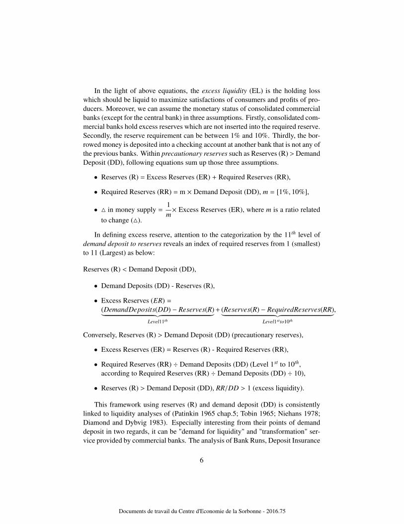
In the light of above equations, the excess liquidity (EL) is the holding loss

which should be liquid to maximize satisfactions of consumers and profits of pro-

ducers. Moreover, we can assume the monetary status of consolidated commercial

banks (except for the central bank) in three assumptions. Firstly, consolidated com-

mercial banks hold excess reserves which are not inserted into the required reserve.

Secondly, the reserve requirement can be between 1% and 10%. Thirdly, the bor-

rowed money is deposited into a checking account at another bank that is not any of

the previous banks. Within precautionary reserves such as Reserves (R) >Demand

Deposit (DD), following equations sum up those three assumptions.

• Reserves (R) = Excess Reserves (ER) + Required Reserves (RR),

• Required Reserves (RR) = m × Demand Deposit (DD), m = [1%, 10%],

• in money supply =1

m× Excess Reserves (ER), where m is a ratio related

to change ().

In defining excess reserve, attention to the categorization by the 11th level of

demand deposit to reserves reveals an index of required reserves from 1 (smallest)

to 11 (Largest) as below:

Reserves (R) < Demand Deposit (DD),

• Demand Deposits (DD) - Reserves (R),

• Excess Reserves (ER) =

(DemandDeposits(DD) − Reserves(R)︸︷︷︸

Level11th

+ (Reserves(R) − RequiredReserves(RR)︸︷︷︸

Level1stto10th

,

Conversely, Reserves (R) > Demand Deposit (DD) (precautionary reserves),

• Excess Reserves (ER) = Reserves (R) - Required Reserves (RR),

• Required Reserves (RR) ÷ Demand Deposits (DD) (Level 1st to 10th,

according to Required Reserves (RR) ÷ Demand Deposits (DD) ÷ 10),

• Reserves (R) > Demand Deposit (DD), RR/DD > 1 (excess liquidity).

This framework using reserves (R) and demand deposit (DD) is consistently

linked to liquidity analyses of (Patinkin 1965 chap.5; Tobin 1965; Niehans 1978;

Diamond and Dybvig 1983). Especially interesting from their points of demand

deposit in two regards, it can be "demand for liquidity" and "transformation" ser-

vice provided by commercial banks. The analysis of Bank Runs, Deposit Insurance

6


and Liquidity (Diamond and Dybvig, 1983) embodies uninsured demand deposit

contracts are able to provide liquidity but leave banks vulnerable to runs. Liquid-

ity is intimated linked with possibility of liquidity that the bank knows how many

withdrawals will occur in demand deposit when confidence is maintained.

The juxtaposition between excess reserve and demand deposit has strong asso-

ciation which underlines the connection between excess liquidity and uninsured

liquidity. The vulnerability of bank runs (Diamond and Dybvig, 1983) occurs be-

cause there are multiple equilibria with differing levels of confidence.

Liquidity role stands to reason that is differ from the Diamond and Dybvig model

(1983). Apparently, for investors, asset liquidity is linked to the market operation

(Jacklin, 1987; Haubrich and King, 1990; von Thadden, 1997; Hellwig, 1994).

On the other hand, it should be added by transaciton between banks and markets.

Uncertainty about amount of liquidity (Diamond, 1997) is useful concept that the

liquid probability of cardinal utility(Diamond, 1997) of consumptions of firms is

started to be argued. However, banks are merely objects having assets should be

melted to be liquid because banks want to be inserted in the market operations.

Nature of the banking industries exists in two sides of assets and liabilities, fur-

thermore, in on balancesheet factors and off balancesheet factors in open market

operations.

Liquidity creation is in two sides of a coin about riskinesses. It can be argued for

liquidity creating riskless and causing the problem in risky asset markets (Gorton

and Pennacchi, 1990). Otherwise, borrowing and lending are permitted but con-

strained (Kehoe and Levine, 2001).

certain outcome uncertain outcome

DD indexDD − R

R

DD − R

DDDD (Demand Deposit) R (Reserves)

RR indexR − RR

RR

R − RR

RRR (Required Reserve)

Table 2. DD Index and RR Index in uncertainty

As above, using two different indexes stands to reason that for certain outcome

in demand deposit (DD) index, how far demand deposit is bigger than reserves, for

uncertain outcome, within the scale of demand deposit, where reserves are located.

Otherwise, for certain outcome in required reserve (RR) index, how far reserves are

bigger than required reserves, for uncertain outcome, within the scale of reserves,

where required reserves are located.

7


2.2. Credit Rationing

Because of non pledgeability of required reserves (RR) in case of bankruptcy,

pledgeable demand deposit (DD) can be marked by RR−DD > 0, required reserves

(RR) will be required for strict positive net present value in banks. Let A be the

excess liquidity of capital at the vortex of precautionary aim.

A ≥ A ≡ RR − DD > 0. (1)

A lower bound A on liabilities and equities of banks invites a reading on sev-

eral levels of understanding. The negative effect of a lower bound A is achieved

through increasing of demand deposit (DD) comparably than required reserves

(RR), DD > RR. Commercial banks need to extend their deposit level paralleled

to demand deposit (DD). On the other hand, central banks require the reserve level

to commercial banks. Admittedly, A lower bound A is credit-rationed.

Figure 2. Positive Credit Rationing (left) and Negative Credit Rationing (right)

For example, demand deposits of commercial banks contain loans, excess re-

serves and required reserves. excess reserves can pay demand deposits incurred by

loans. The composition between excess reserves and loans can be arranged. All

in all, central banks have commercial bank reserves as liabilities. In some specific

cases, required reserve rate is the percentage of deposit in demand deposit. At all

events, reserve amount should cover the demand deposit for credit rationing. A

commercial bank is overnight interbank interest player in a case of

A < R − DD. (2)

Why would a commercial bank hold excess reserves at the central bank? The

motivation to hold excess reserves has relevance to make more networks between

small banks and a big bank. For example, a small bank Tiny has lent more money

than they intended so some of expected incoming funds did not arrive timely. A

8


small bank Tiny faces the problematic situation of liquidity shortage to meet the

required reserve supposed to be sent to the central bank. On the other hand, a big

bank Too Big Too Fail has excess cash. A big bank Too Big Too Fail is supposed

to lend to a small bank Tiny. An announcement "I lend you" by a big bank Too

Big Too Fail executes an overnight wire so a small bank Tiny can meet the required

reserves at the end of day. Indeed, overnight wire isn’t a wire of cash between

banks. It is a wire of cash to reserves of a central bank paralleled to loans of a

small bank Tiny. Consequently, commercial banks’ excess reserves are involved

in reserves of central banks. Generally speaking, bank size is maintained. For an

excess reserved bank, a change of excess reserves in the composition of a balance

sheet is less risky when it is involved in reserves of central banks.

In spite of rearrangement at the balancesheet composition, excess liquidity has

positive value than low bound A because excess liquidity contains cash vaults and

ATMs beyond excess reserves.

R − RR ≥ R − RR − A, (3)

In spite of easy deduction with excess liquidity A, being able to transfer cash

payoffs does not imply that utility is transferable: wealthy and poor players may

derive a different utility from the same amount of money. If capital is credit ra-

tioned at the low bound A, the utility payoff U of banks shows satisfaction about

funding value to hold excess liquidity A depending upon utility jumps at A = A.

U =

A + R − RR, if A ≥ A ,

A, if A < A .(4)

To put it differently, the difference between excess liquidity A and low bound

A implies tolerance level of excess cash. The candidate to achieve low bound A

(=RR−DD) can be proper amount of cash holdings. Because required reserves are

various, I am puzzle on the important scale between the precautionary reserve and

the decision to hold excess funds for hedging liquidity confronting risky situation

like wars and terrors which is different at each country. In case of only A left in the

payoff utility if A < A, that is DD − RR > 0, banks want to bet more on hazardous

liquidity A. Simultaneously, the risk-averse bank turns into the risk-taking invest-

ment plan.

The moral hazard problem occurs when the poor status of borrowing banks is neg-

liged by lending banks. Let A ≡ DD − RR > 0 be the scale of the hazardous

liquidity, let ρ0 be the total expected return of pledgeable DD−R, and ρ1 the return

of excess R − RR, both measured per unit invested.

9


Figure 3. Excess Demand Deposit (DD) and a Negative Wedge Z1 − Z0 (rent)

0 RR R(Z1) DD(Z0)ρ1 ρ0

identification symbols: RR (Required Reserves), R (Reserve), DD (Demand Deposit)

Thus, A results in a total payoff (ρ0 + ρ1) × A of which ρ0 can be pledged to

outside investors. The residual ρ0 × A is the minimum rent of overnight investment

plan to the bank.

ρ1 = pH × R,

ρ0 = pH × (R −B

ρ0

),(5)

where pH is denoted as the probability of success, B as the return of a bad plan and

R as return.

The rational bank expects the return from overnight investment plan. Hence,

we get:

0 < ρ1 < 1 < ρ0. (6)

Consequently, the bank has the minimum illiquidity ratio:

1 − ρ1, (7)

Maximum betting level for excess liquidity investment plan is:

A ≡ DD − RR

1 − ρ1

. (8)

and gross payoff is:

Ug =(ρ0 − ρ1) × A

1 − ρ1

= µA, (9)

where

µ ≡ρ0 − ρ1

1 − ρ1

(10)

10


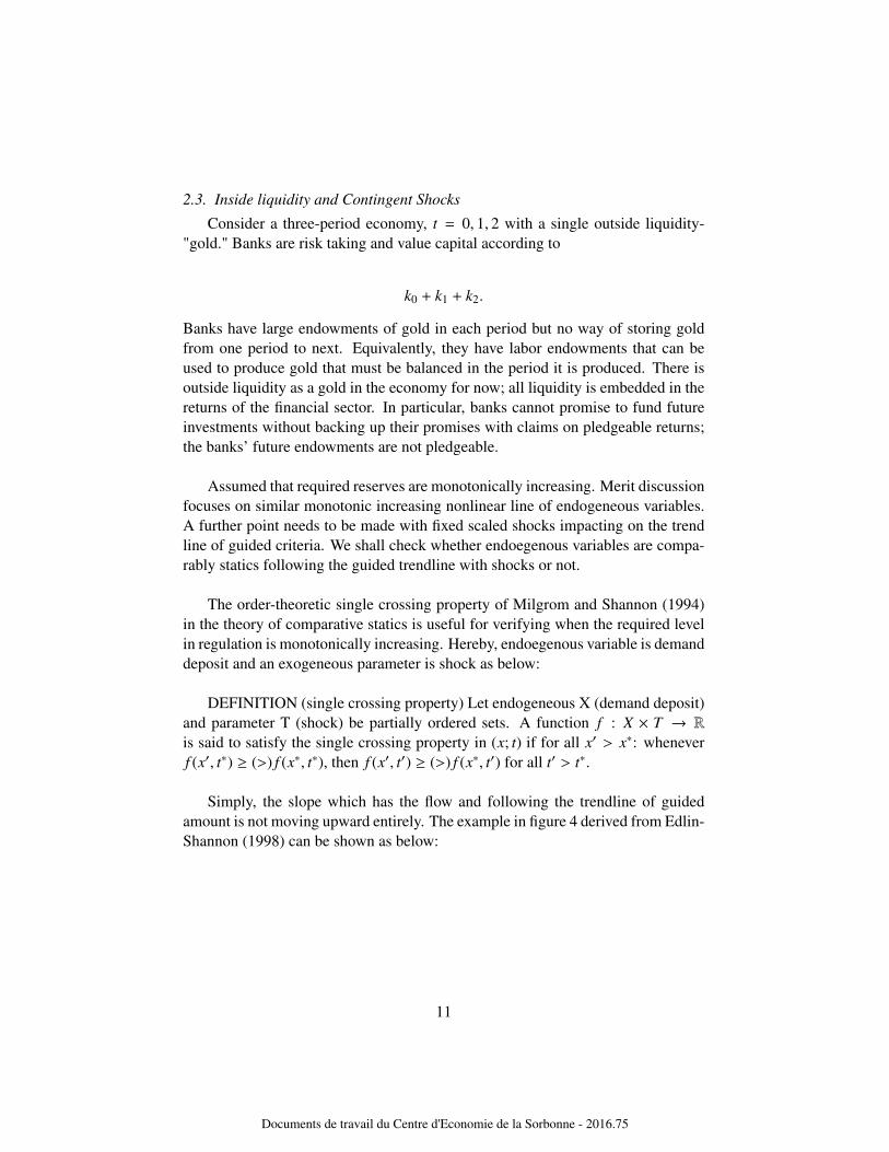
2.3. Inside liquidity and Contingent Shocks

Consider a three-period economy, t = 0, 1, 2 with a single outside liquidity-

"gold." Banks are risk taking and value capital according to

k0 + k1 + k2.

Banks have large endowments of gold in each period but no way of storing gold

from one period to next. Equivalently, they have labor endowments that can be

used to produce gold that must be balanced in the period it is produced. There is

outside liquidity as a gold in the economy for now; all liquidity is embedded in the

returns of the financial sector. In particular, banks cannot promise to fund future

investments without backing up their promises with claims on pledgeable returns;

the banks’ future endowments are not pledgeable.

Assumed that required reserves are monotonically increasing. Merit discussion

focuses on similar monotonic increasing nonlinear line of endogeneous variables.

A further point needs to be made with fixed scaled shocks impacting on the trend

line of guided criteria. We shall check whether endoegenous variables are compa-

rably statics following the guided trendline with shocks or not.

The order-theoretic single crossing property of Milgrom and Shannon (1994)

in the theory of comparative statics is useful for verifying when the required level

in regulation is monotonically increasing. Hereby, endoegenous variable is demand

deposit and an exogeneous parameter is shock as below:

DEFINITION (single crossing property) Let endogeneous X (demand deposit)

and parameter T (shock) be partially ordered sets. A function f : X × T → R

is said to satisfy the single crossing property in (x; t) if for all x′ > x∗: whenever

f (x′, t∗) ≥ (>) f (x∗, t∗), then f (x′, t′) ≥ (>) f (x∗, t′) for all t′ > t∗.

Simply, the slope which has the flow and following the trendline of guided

amount is not moving upward entirely. The example in figure 4 derived from Edlin-

Shannon (1998) can be shown as below:

11


Figure 4. Comparative statics in investment

Comparative statics in investment is the comparison of two different pledgeable

portpolios, before and after a change of an exogeneous shock within fixed scale by

credit rationing. Here by, credit rationing is specified in the gap between insured

amount and parameterized amount: pledgeable demand deposit and required re-

serves. The excess liquidity composed by excess reserves is a kind of a shock.

The exogeneous shock is measured by demand deposit index and required reserve

index obtained by credit rationing.

To reach a easier understanding of credit rationing, assume that required reserve

(RR) of a bank is monotonically increasing. Certainly, the aim of soft regulation

is to check comparatively statics to sufficiently follow the trend of guideline. not a

limitation of specific guideline about an amount.

Therefore, when we check the change when the slope is increasing, the change

before shock and one with shock increase. However, the change is not beyond

the required reserve line. Change is comparably statics but it shows increasing is

vigorously continous along monotonic increasing of criteria for regulation. There

remains a range of problems to be tackled because shocks in investment have com-

parativly statics so it can be nonlinear motions but the lending contract has the fixed

term which can be seen in the linear approximation.

2.4. Net lending: The case of certainty

At date 1, the liquidity shock ρ ≥ 0 takes place. Let i(ρ) ≤ RR denote the con-

tinuation scale and at least shock can cover the worst scenario, ρ0 < ρ. Remark that

ρ1 = pH × R,

ρ0 = pH × (R −B

ρ0

),(11)

12


where pH is denoted as the probability of success, B as the return of a bad plan, R

as return.

We assume the high liquidity shock is fL = 1 and ρH = ρ. Further, 1 + ρ < ρ1,

implying that the betting on overnight plan would always be worth undertaking

from a net present-value point of view. If there are no liquidity problems, a bank

with funds A ≡ DD − RR transfers certain amount to the central bank as follows at

date 0: He chooses RR as the initial scale of the project and invests (ρ−ρ1)×RR > 0

into a liquid asset or a credit line, where RR is set to exhaust the budget, (1 + ρ −

ρ0) × RR = A. With these initial investments the bank is able to cover exactly the

deterministic liquidity shock ρ at date 1. He can raise ρ1 × RR by making an angel

loan against his pledgeable date-2 deposits and add to it his portfolio in liquidity

(ρ − ρ1) × RR.

The plan presumes that there is a liquid assert, or a credit line backed by a liquid

asset, that allows the bank to save (ρ− ρ1)× RR from date 0 to date 1. However, in

the economy just described, the only available assets are claims on the continuation

value of banks looking to save. Suppose, hypothetically, that all banks are able to

meet the date-1 liquidity need ρ × RR and therefore to continue at full scale. Then

the date-1 continuation value of the financial sector is ρ1 × RR. But this is less

than the liquidity needed, ρ×RR. Since, the net continuation value of the financial

sector, (ρ1 − ρ) × RR, is negative, consequently the financial sector can neither act

as a store of value nor provide collateral for future funding by institution.

This is itself emblematic of certain inside liquidity. Lending can be tied to the

duration by fixed contract given five years or more. In detail, complete information

about returns of portfolio is revealed in the loan contract. By contrast, preference

of banks is incomplete information in comparative statics. Suffice it to say that this

requires uncertainty methodology which can be better in a pictorial way for easier

explanation.

2.5. Selected Liquid Characteristics of Village I and Village II

Having outlined the institutional context dealing with different countries, the

discussion now turns to the real economy. In order to provide a framework for

more detailed consideration of credit rationing, it will be helpful to compare two

villages. There is a marked contrast between a village I holding a small reserve

(reserve ratio 7%) and a village II holding an excess reserve (reserve ratio 30%).

To a great extent, within the outside liquidity system, both village I and village II

are conceived of excess liquidity (7867, 44800) : ≡ currency issued (5886, 400,

current USD, million) + excess reserve (1981, 44400, current USD, million).

13


(Current USD, million) Village I Village II

Outside Liquidity in domestic currency, liabilities

currency issued 5,886 400

required reserve 2,053 19,200

excess reserve 1,981 44,400

reserve money 9,920 64,000

demand deposit, commercial banks 12,684 3,028

excess liquidity R < DD DD < R

Inside Liquidity

overnight deposit window rate 2.75 2.75

credit rationed A -10,631 60,972

domestic credit to private sector by banks to GDP (%) 70 99.2

net commercial bank lending and other private credits 250 -43

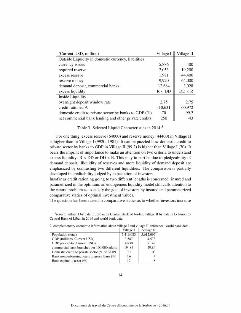
Table 3. Selected Liquid Characteristics in 2014 5

For one thing, excess reserve (64000) and reserve money (44400) in Village II

is higher than in Village I (9920, 1981). It can be puzzled how domestic credit to

private sector by banks to GDP in Village II (99.2) is higher than Village I (70). It

bears the imprint of importance to make an attention on two criteria to understand

excess liquidity: R < DD or DD < R. This may in part be due to pledgeability of

demand deposit, illiquidity of reserves and more liquidity of demand deposit are

emphasized by contrasting two different liquidities. The comparison is partially

developed in creditability judged by expectation of investors.

Insofar as credit rationing going to two different lengths is concerned: insured and

parametrized in the optimum, an endogenous liquidity model still calls attention to

the central problem as to satisfy the goal of investors by insured and parameterized

comparative statics of optimal investment values.

The question has been raised in comparative statics as to whether investors increase

5source: village I by data in Jordan by Central Bank of Jordan, village II by data in Lebanon by

Central Bank of Liban in 2014 and world bank data.

2. complementary economic information about village I and village II, reference: world bank data.

Village I Village II

Population (total) 7,416,083 5,612,096

GDP (millions, Current USD) 3,587 4,573

GDP per capita (Current USD) 4,830 8,148

commercial bank branches per 100,000 adults 19. 85 29.84

Domestic credit to private sector (% of GDP) 70 103

Bank nonperforming loans to gross loans (%) 5.6 4

Bank capital to asset (%) 12 8

14


the amount of investment or not. Our concern is not with the increase of broad in-

vestment amount which can be credited but with insured and parametrized amount

getting to the optimal value.

A richer analysis of the interdependence between the excess liquidity and credit

rationing components in the spread between pledgeable and unpleageable amount

for different countries can be carried out by considering the government policy rule

changing the mix of assets held by the private sector through open market opera-

tions (Kiyotaki-Moore, 2008).

For example, a look at functioning of the economy by the central bank’s balance

sheet, Garreth (2015) argues on impact of central bank collateral choices in Bank

of England caused by the Asset Purchase Facility (APF) reaching 375 billion by

late 2012.

Additionally, a clue to changes of asset composition is provided by numerous styl-

ized facts about the asset purchases and the freshly created reserves in Hong Kong

(long-standing currency peg regime since 2005 by Hong Kong Monetary Author-

ity (HKMA) and Thailand (inflationary targeted (0.5-3.0%) operational strategy to

absorb excess liquidity by market.

There can be little doubt that offset in the same composition is always possible in

the changeable composition. The change of positioning in the same frame figura-

tive as the change of a composition carries articulation of flows. By the way, this

framework requires heavy emphasis on the proof that the value of investment has

single-valued because the value can be representable in the balance sheet. The puz-

zle on offset among different values obtained by credit rationing sets the tone for

investment having multi-dimensional valued regardless of on-balancesheet factors

and off-balancesheet factors.

2.6. Composition of Liquidity

At the heart of credit rationing lies the conception of the liquidity composition.

In relation to what I have previously said that Village I and Village II are having

excess liquidity as far as excess cash and excess reserves concerned. In detail, even

though the measurement of excess cash is not easy, Village I are having the excess

reserve than required reserves (3340 > 694). Likewise, Village II are having the

excess reserves than required reserves as well as Village I (44400 > 19200). By

the way, a closer look at the compositon with credit rationing, demand deposit -

required reserves (-1764 , 16172) gives a different answer.

15


Village and Credit Rationing, Certainty, Precautionary Uncertainty,

Liquidity I : -(DD-R) excess liquidity Level Index inside liquidity

Composition II: RR-DD I: (R-RR) ÷ R (Lowest 1- I: (DD-R) ÷ DD

II: (R-RR) ÷ RR Highest 11) II: (DD-R) ÷ R

Village Village I, II Village I, II Village I, II Village I , II

currency issued 5886 , 400

required reserve 694 , 19200

reserve ratio 7% , 30%

excess reserve 3340, 44400

reserve money 9920, 64000

demand deposit 12684 , 3028

credit rationing -11990 , 16172

excess reserve 1981 (actu), 44400

(R-RR) ÷ RR 93 % , 233 %

Level Index level 11

(DD-R) ÷ R 22%, -0.0084 %

Table 4. Composition of Village Liquidity in 2014

identification symbols: DD (Demand Deposit), R (Reserve), RR (Required Reserves),

source: village I by data in Jordan by Central Bank of Jordan, village II by data in Lebanon by Central Bank of Liban in 2014 and world bank data.

Seen in the perspective of an asset-liability match, demand deposit exerted a

strong influence on reserves. It is not seem to rash to suggest required reserves as a

percentage of net demand deposits held in commercial banks by customer. Demand

deposit against reserves is total demand deposits less "due from" (Allen, 1956). No

single explanation can account for the single driver to describe the change of re-

serves with credit and demand deposit. However, Several assumptions are worth to

be mentioned for the sake of financial regulation.

It is not unreasonable to postulate that credit rationing is differently interpreted as a

transaction holding a liability (Henderson, 1960), reserve credit (Allen, 1956) and

a monetary instrument (Siegel, 1981). It can be a transaction (Henderson, 1960)

for a borrower occupied by the federal funds absorption ratio of a financial liabil-

ity defined as the amount of federal funds which directly and indirectly support a

one-dollar public holding of the liability. As a matter of the fact, a country bank

allows a reserve city bank with different reserve requirements by shifting interbank

deposits depending upon reserve credit (Allen, 1956) because the total reserve is

not changed and only distribution among banks by shifts in interbank balances.

Additionally, as a monetary instrument, optimal reserve requirement on demand

deposits (Siegel, 1981) controls the value of monetary aggregates.

As a closer look at the composition of Village Liquidity in 2014, credit rationing

of Village I (R < DD = 9920 < 12684) is negative and on the other hand, Village

16


II (R > DD = 64000 > 3028) is positive. It indeed may be said with safety that

motivation to hold liabilities excessively is purely surplus reserves in 1930 with-

out any economic purpose caused by lack of good loan opportunities. After crisis

2007, good loan opportunities hinges on a series of remedies in a bad economic

situation up to one country and more.

Passively accumulated excess liquidity is not merely explained by the conservative

banking system. At the same time, as a meaning of proper loan commitment, it is

no less dubious to connect that the bank behavior in the uncertain situation should

be viewed with reservation. It is no wonder the motif to hold excess liquidity is

good reason to show credit facility to induce good loan opportunities and obtain

safer investment return by overnight interest. This motivation requires a quite log-

ical explanation with small sample of reserves in a vulnerable economy.

3. Inside Liquidity in a Machina’s Triangle

A further point needs to be made with regard to inside liquidity. This part will

be a step toward a richer and more inclusive understanding of the ease with which

investors can obtain funding. With problems to deal with potential outcomes re-

sulting from funding, expected value needs to be calculated with cardinal utility

function before revealed preference.

Measurement of cardinal utility function needs to look more closely at the interval

scale. Now for an example of three events which the event A and B are uncertain

to occur and C is certain to occur:

P(A or B and C) = P(A ∪C) + P(B ∪C)

In this discussion, when we say "A or B and C occur" we include three possi-

bilities:

1. A occurs, B does not occur and C does occur,

2. B occurs, A does not occur and C does occur,

3. C occurs, A does not occur and B does not occurs.

This use of the word "or" is technically called exclusive because it does not

include the case in which both or more events occur at the same time.

Here are two worlds in antithesis. By and large, probabilities of various out-

comes arising from any chosen alternative are objectively known. Conversely, a

lottery representing risky alternatives might be monetary gambles on the spin of

an unbiased roulette wheel. Furthermore, compound lotteries (L1, ..., Lk;α1, ..., αk)

(MWG, session 6.B) is the risky alternative that yields the simple lottery ℓk with

probability αk for k = 1, ...,K, given K simple lotteries ℓk = (pk1, ..., pk

N), k =

17


1, ...,K, and probabilities rk > 0 with∑

k αk = 1. We can specify compound prob-

abilities with two uncertain events and a certain event in the following example.

Table 5. compound probabilities with heterogeneous valued weighted measure

EXAMPLE : The agent can carry fruits on the plate within three fruits. Letting

event A be an apple, event B be a banana and event C be a coconut on a plate. The

agent prefers three choices: an apple (a) to a banana (b) to a coconut (c). Three

events by each choice are: A ≻ B ≻ C. However, if the preference has the cardinal

value which can be numerical interpretation, then ordinal interpretation can be

challenged because it can have the homogeneity like:

P(r) × P(A) + P(r) × P(B) + P(r) × P(C) = 1

However, whether the weighted measure P(r) is homogenous or not, the

probability measure space ω = P(r) × P(A) + P(r) × P(B) + P(r) × P(C) is

different. In case of homogenous valued weighted measure P(r) = 1/10 and each

P(A) = 1/2, P(B) = 1/3, P(C) = 1/6 has combined measure space 1. In case of

heterogeneous valued weighted measure at P(r), combined measure space is not 1.

How we can intepret risk preference when compound measure space is not 1. The

lottery at the origin can be assumed that86

100is certain.

We shall start by an attempt to define independence axiom (Von Neumann and

Morgenstern, 1944) and preferential consequentialism (Vergopoulos, 2011) from

certain probability methodology to uncertainty. for the risk preference A ≻ B ≻ C,

the origin point has less riskier and certain value, C. The lottery point C in the y-

axis is more riskier and uncertain value than B in the x-axis. Binary choice B or C

is described in the half space of rectangular shaped space which is like a triangle

because compound probabilities are not jointed but weighted. If we imagine the

game tree, several subgame trees exist independently:

1) The preference relation on the space of simple lotteries ℓ satisfies the in the

independence axiom if for all L, L′, L” ∈ ℓ and α ∈ (0, 1), we have L L′ if and

only if αL + (1 − α)L” αL′ + (1 − α)L”

18


2) Preferential consequentialism is that the agent firstly recognizes the

endogenous event (E), regardless of the preferred act g in the exogenous event

(Ec), he will choose the preferred act f in the endogenous event (E): fEg ∼E f .

3) Savage’s Sure Thing Principle (STP) (Savage 1954; Aumann, Hart): For any

event E ⊂ Ω and any acts f , g, h, k ∈ B(Ω), fEh 0 gEh↔ fEk 0 gEk where 0 is

an optimal ex ante choice in the backward induction.

4) Dynamic Consistency: For any information structure (Ei)1≤i≤n and any acts

f , g ∈ B(Ω), ∀i ∈ [1, n], f Eig⇒ f 0 g. Additionally, if f ≺Ei

g for some i

such that Ei is not null, then f ≺0 g.

By the independence axiom, the agent should choose the first lottery (L) than

the second lottery (L’) regardless of the third one (L"). Excess liquidity is not as

compelling to be needed for the analysis in the presence of certainty as it is under

uncertainty. Machina’s paradox (1987) is an interesting technique to demonstrate

the influence of "what might have been." on consequences which is the violation of

the independence axiom. The independence axiom sets out examine the more ob-

scure and puzzling aspect of the third lottery. The order of two lotteries by certain

preference does not depend on (is independent of) the appearance of the particu-

lar third lottery. Significantly, particular certain event has increasing importance

by the preference indifference in the preferential consequentialism. In that, any

event E is the subset of a finite set of information structure Ω. Among any atomic

act set f , g in the information structure Ω, the act fEg is conditionally defined by

"( fEg)(ω) = f (ω) if state ω ∈ E" and "( fEg)(ω) = g(ω) if ω ∈ Ec."

EXAMPLE (independence axiom): There are three outcomes: "a trip to New-

york," "eating a New-york styled bagel," and "staying in the office. " Suppose that

you prefer the first lottery to the second one and the second one to third one. The

choice to select the second lottery is rational if you anticipate that you cannot travel

to New-york. However, the independence axiom forces you to prefer the first lot-

tery to the second one (Machina Paradox in section 6.B, MWG).

EXAMPLE (Preferential consequentialism) : You are invited for a dinner (E).

You were supposed to drink a Beer (g) in case of staying at home (Ec). However,

you decide to carry a Wine ( f ) for an invitation of dinner(E).

A prospect is a point (A, B, C, D in a certain year) in a triangle. Consider the

four prospects A, B, C and D. Note that the slope of the line CD is (1 − a)(1 −

b)/a(1 − b) = (1 − a)/a. This is also the slope of the line AB. We assume that

the independence axiom implies that indifference curves are parallel lines. Thus, if

D ≻ C, then expected utility must be rising along the line AB in the direction of B.

19


Conversely, if D ≺ C, then expected utility must be decreasing along the line AB.

Supposed by the 45 degree slope and the point value in a specific year, a = 0.5,

b = 0.43 are contributed to calculate four prospects are as follows:

A = (0, 1, 0)

B = (1/2, 0, 1/2)

C = (0, 0.43, 0.57)

D = (0.285, 0, 0.715)

As we can see at B (1/2, 0, 1/2) and D (0.285, 0, 0.715), if the point is the

remotest from the origin point A, then the probability is 0 at the state 2 of certain

outcome x2.

Figure 5. Remoted prospects from the origin point

Dynamic consistency is to maintain dynamics of ex post preference to select

acts in case of the event (E), then the optimal ex ante preference by backward

induction also follows same dynamics. Under preferential consequentialism, stan-

dard arguments of non-consequential theories (e.g. Machina 1989; Epstein and Le

Breton 1993; Hanany and Klibanoff 2007; Vergopoulos, 2011, proposition 1) al-

lows us to assume that violation of Sure Thing Principle implies dynamic inconsis-

tency. The slopes of indifference curves indicate the individual’s relative sensitivity

20


to changes in p1 versus changes in p3, are given by MRS(x2 → x3, x2 → x1) =

(U(x2; Fp1,p3)−U(x1; Fp1,p3

/U(x3; Fp1,p3−U(x2; Fp1,p3

)). A steeper slope indicates

a higher level of risk aversion. More risk averse of the local utility function raises

the slope of the indifference curves. The indifference curves will appear "fanned

out" (Machina, 1982) so that the relatively steeper slopes in the (p1, p3) plane near

the vertical axis than in the one near the horizontal axis illustrates the individual’s

greater sensitivity to changes in p1 relative to p3 when p1 is small relative to p3,

and vice versa.

Figure 6. risk preference and steeper slopes by fanned out

The precautionary reserve locates on the origin point which is not an argument

in uncertain outcome framework. Here by the argument is steeper slopes in the

(p1, p3) plane near the vertical axis which represents risk preference. Because the

logic of risk preference is outcome might be happened riskier so that the return of

riskier choices is expected greater than the choice in the origin point. Remarked

with two index, DD index (DD-R)/DD and RR index (R-RR)/R, the point of the

demand deposit (DD) index at the vertical axis than one of the required reserve

(RR) index at the horizontal axis raises the slope of the indifference curves.

4. Empirical founding in the case of Jordan and Lebanon during the period

1993-2015

This part takes a systemic and comprehensive approach from excess liquidity

to surplus liquidity with the case of Jordan and Lebanon during the period 1993-

2015. The MENA (Middle East and North Africa) region has passed political and

economic conflicts since the Gulf war in 1990 and 1991 located on Iraq, Kuwait,

Saudi Arabia and Israel. It affects Jordan as a small open oil-importing country

who is geographically in Southwest Asia, south of Syria, west of Iraq, northwest

21


of Saudi Arabia and east of Israel and the West Bank. As time goes by, conflict

areas neighbored with Jordan are seemed to have higher risk in finance. Especially,

liquid asset is spotlighted to be sent to a safer country Jordan and Lebanon by res-

idents in conflict areas.

Net lending in conflict areas is higher for restoration from the war. Ostensibly,

the confusion among net lending, grant and excess liquidity is bolded than before

1993. In case of Jordan, the holdings rate which is the exchange rate of a currency

against the special drawing right (SDR) derived from the currency’s representative

exchange rate reported by the central bank, is consistently about 1 from 1991 up

to 2016, radically decreasing from 2.5 in 1985. In detail, remoted from the im-

pact from the war, for the period (2009 – 2015), basic spread in financial sectors

in jordan: deposit interest rate, lending rate are consistently maintained from 4%

to 5% regarding to the bank lending-deposit spread. The deposit interest rate de-

creases from 4.8% in 2013 to 3.49% in 2015. In addition, the lending interest rate

decreases from 9.01% in 2013 to 8.47% in 2015 as well.

Real interest rate fluctuates even though there is stability of deposit interest rate,

lending rate and interest spread during 2003-2015. For economic financial stabil-

ity, in all probability, understanding liquidity in financial sector and remittance and

transaction in external sector is important than ever to analyze imbalanced part in

Jordan.

According to S.Gray (2006), excess reserves are described the position of most

developed country central banks: the Bank of England, the US Federal Reserve

Bank, the European (System of) Central Banks and the Bank of Japan. In addition,

it could be the case that the surplus is represented by excess cash in circulation

(supply is greater than demand) rather than by commercial bank balances at the

central bank; this is unlikely although it can be observed in a few countries. In

case of Jordan, this is the case of excess cash. On the other hand, cash is on deficit

as the percentage of GDP Regarding reserve money which contains currency and

reserves in central bank of Jordan, issued currency composed the major part of

reserve money during the period (2013-2015) and approximated 60% on average.

Issued currency increased from 3559 Jordanian million dinars in 2012 to 4336

Jordanian million dinars in 2015 and reserve money as well increased from 5229

Jordanian dinars in 2013 to 7505 Jordanian dinars in 2015.

Middle East and North Africa (MENA) after the Gulf war from 1990 and 1991

can access to get good loan opportunities: debt forgiveness. It is of course not

needed to say laziness of conflict countries to be vulnerable by external shocks in

their economies. To put it differently, the exact probabilities to indicate the bank

behavior in spite of short time series data which cannot be shocked durably and

sequentially up to future, better put, the worst situation is happened and should be

recovered by net lending, should be noted.

22


5. Summary

Credit rationing is rationing of excess liquidity by risk preference on compara-

ble statics of liquid investment. This study addressed two research questions: First,

the key question to be asked is how a subject of excess reserves in excess liquidity

after the banking crisis of the early 1930s or 1970 can be re-identified in 2016. And

second, needs of new technique about risk preference provides a useful ground to

test the cross-sectional data between economics and finance by applying theories

about uncertainty which is hereby the Machina’s triangle (1982, 1987). For one

thing, Excess liquidity has simply deduced itself from required reserves in banks.

By the way, if Increasing credit rationing at the precautionary level stand out from

the gap of required reserves and pledgeable demand deposit, RR−DD > 0. Not the

least of these is its mixture of styles, increasing credit rationing at the aim of in-

vestment is within fixed reserve scale, Reserves (R) - Demand Deposit (DD). Most

obviously, risk preference in the triangle distinguishes between risky loving behav-

ior inside of a triangle and risk aversion behavior at the origin. As has been noted

earlier, comparative statics in investment is a richly detailed study of the nature of

monotonic required regulation criteria. Especially important is hard regulation on

increasing the precautionary level is impossible to quibble with increasing every

level set above required level. Consequently, the aim of soft regulation is to check

comparatively statics to sufficiently follow the trend of guideline. not a limitation

of specific guideline about an amount. This technical result of my study point to

several promising applications for regulatory issues.

23


6. (Annex)

6.1. Village I (Jordan)

identification symbols: DD (Demand Deposit), RR (Required Reserves), R (Reserve), EL=Excess Liquidity

Year DD-RR/R R-RR/RR, Precautionary Reserves RR/DD, RR index (1-11th)

1993 -35% 567%,certain outcome 23%,3th(below 30%)









2002 1% 92%,uncertain outcome 11th(over 100%)






2008 0% 91%,certain outcome 1th(below 10%)








24


6.2. Risk preference description in the Machina Triangle

Village I (Jordan)

Framework of risk preference in the Machina Triangle

25


6.3. Village II (Lebanon)

identification symbols: DD (Demand Deposit), RR (Required Reserves), R (Reserve), EL=Excess Liquidity

Year DD-R/R R-RR/RR, Precautionary Reserves RR/DD, RR index (1-11th)


1994 -82% 233%,certain outcome 166,11th






















7. Bibliography

Allen, W. R. (1956). Interbank Deposits and Excess Reserves. The Journal of Finance,

11(1), 68. doi:10.2307/2976530.

Blanchard, O. (2007). Current Account Deficits in Rich Countries. doi:10.3386/w12925.

Brunnermeier, M., Pedersen, L. H. (2008). Market Liquidity and Funding Liquidity.

doi:10.3386/w12939.

Cressy, R. (2002). Introduction: Funding Gaps:. The Economic Journal, 112(477).

doi:10.1111/1468-0297.00680.

Diamond, D. W., Dybvig, P. H. (1983). Bank Runs, Deposit Insurance, and Liquidity.

Journal of Political Economy, 91(3), 401-419. doi:10.1086/261155.

Diamond, D. (1997). Liquidity, Banks, and Markets. Journal of Political Economy,

105(5), 928-956. doi:10.1086/262099.

Edlin, A. S., Shannon, C. (1998). Strict Single Crossing and the Strict Spence-

Mirrlees Condition: A Comment on Monotone Comparative Statics. Econometrica, 66(6),

1417. doi:10.2307/2999623

Frost, P. A. (1971). Banks’ Demand for Excess Reserves. Journal of Political Econ-

omy, 79(4), 805-825. doi:10.1086/259789.

26


Garreth, R. (2015). Centre for Central Banking Studies Handbook – No.32 Under-

standing the central bank balance sheet. Bank of England.

Gorton, G., Pennacchi, G. (1990). Financial Intermediaries and Liquidity Creation.

The Journal of Finance, 45(1), 49-71. doi:10.1111/j.1540-6261.1990.tb05080.x.

Gray, S. (2011). Central Bank Balances and Reserve Requirements. IMF Working

Papers, 11(36), 1. doi:10.5089/9781455217908.001.

Gray, S., Karam, P., Ariss, R. T. (2014). Are Banks Really Lazy? Evidence from Mid-

dle East and North Africa. IMF Working Papers, 14(86), 1. doi:10.5089/9781484386460.001.

Haubrich, J. G., King, R. G. (1990). Banking and insurance. Journal of Monetary

Economics, 26(3), 361-386. doi:10.1016/0304-3932(90)90003-m.

Hellwig, M. (1994). Liquidity provision, banking, and the allocation of interest rate

risk. European Economic Review, 38(7), 1363-1389. doi:10.1016/0014-2921(94)90015-9.

Henderson, J. M. (1960). Monetary reserves and credit control. Amercian Economic

Review, 348-369.

Holmstrom, B., Tirole, J. (1996). Private and Public Supply of Liquidity. doi:10.3386/w5817.

Holmstrom, B., Tirole, J. (2011). Inside and outside liquidity. Cambridge, MA: MIT

Press.

Jacklin, C. J. (1984). Demand deposits, trading restrictions and risk sharing. Chicago,

IL: Center for Research Security Prices, Guaduate School of Business, University of Chicago.

Kehoe, T. J., Levine, D. K. (2001). Liquidity Constrained Markets Versus Debt Con-

strained Markets. Econometrica, 69(3), 575-598. doi:10.1111/1468-0262.00206.

Kiyotaki, N., Moore, J. (2012). Liquidity, Business Cycles, and Monetary Policy.

doi:10.3386/w17934.

Kopecky, K. J. (1984). Monetary Control under Reverse Lag and Contemporaneous

Reserve Accounting: A Comparison: Comment. Journal of Money, Credit and Banking,

16(1), 81. doi:10.2307/1992652.

Machina, M. J. (1982). "Expected Utility" Analysis without the Independence Axiom.

Econometrica, 50(2), 277. doi:10.2307/1912631.

Machina, M. J. (1987). Choice Under Uncertainty: Problems Solved and Unsolved.

Journal of Economic Perspectives, 1(1), 121-154. doi:10.1257/jep.1.1.121.

Milesi-Ferretti, G., Blanchard, O. (2009). Global Imbalances: In Midstream? IMF

Staff Position Notes, 2009(29), 1. doi:10.5089/9781462333387.004.

Milgrom, P., Shannon, C. (1994). Monotone Comparative Statics. Econometrica,

62(1), 157. doi:10.2307/2951479

Niehans, J. (1978). The theory of money. Baltimore: Johns Hopkins University Press.

Patinkin, D. (1965). Money, interest, and prices; an integration of monetary and value

theory. New York: Harper Row.

Saxegaard, M. (2006). Excess Liquidity and the Effectiveness of Monetary Policy: Ev-

idence From Sub-Saharan Africa. IMF Working Papers, 06(15), 1. doi:10.5089/9781451863758.001.

Siegel, J. J. (1981). Bank Reserves and Financial Stability. The Journal of Finance,

36(5), 1073-1084. doi:10.1111/j.1540-6261.1981.tb01077.x.

Thadden, E. V. (1997). The term-structure of investment and the banks’ insurance

function. European Economic Review, 41(7), 1355-1374. doi:10.1016/s0014-2921(96)00030-

x.

27


Tobin, J. (1965). The theory of portfolio selection in The Theory of Interest Rates.London:

Macmillan.

28


Date post:	06-Apr-2022
Category:	Documents
Upload:	others
View:	4 times
Download:	0 times