Economics of silvoarable systems using LER approach T, Borrell 1 , C. Dupraz 1 , and F, Liagre 2 1 Institut National de la Recherche Agronomique, Montpellier, France 2 Assemblée Permanente des Chambres d’Agriculture, Paris, France Mars 2005
Transcript
Economics of silvoarable systems usingLER approach
T, Borrell1, C. Dupraz1 , and F, Liagre2
1Institut National de la Recherche Agronomique, Montpellier, France
2Assemblée Permanente des Chambres d’Agriculture, Paris, France
1 THE LER APPROACH ............................................................................................................4
LER-BIOMASS AND LER-PRODUCT .................................................................................................4THE LER-BASED GENERATOR .........................................................................................................4A WISE HYPOTHESIS FOR THE AGROFOREST TREE GROWTH ..............................................................5MAXIMUM EXPECTABLE LER IN FUNCTION OF SPECIES AND FINAL DENSITY....................................7IMPACT OF THE TGA ON THE LER RESULTS ....................................................................................8
2 DATA REFERENCES AND MAIN HYPOTHESIS ...............................................................9
THE FORESTRY REFERENCES ...........................................................................................................9REFERENCE DATA IN AGRICULTURE ................................................................................................9THE PROFITABILITY THRESHOLD YIELD ......................................................................................... 11MAIN MANAGEMENT FEATURES OF THE AGROFORESTRY SYSTEMS ................................................ 12ECONOMIC HYPOTHESIS ................................................................................................................ 13
CAP payments ........................................................................................................................... 13Tree grants................................................................................................................................ 13Costs and prices ........................................................................................................................ 14
3 MAIN RESULTS .................................................................................................................... 15
LABOUR IMPACT FOR ONE SILVOARABLE HECTARE........................................................................ 15PREDICTION OF YIELD EVOLUTION ................................................................................................ 15
Evolution of the cash flow at the plot scale ............................................................................ 18Influence of the CAP payment policy .................................................................................... 19Evolution of the cash flow at the farm scale ........................................................................... 19
PROFITABILITY OF A SILVOARABLE INVESTMENT .......................................................................... 20Comparing a silvoarable scenario with agricultural scenario .................................................... 20Influence of the TGA on the Agricultural Value ......................................................................... 22Which density to plant to get the best profitability? .................................................................... 22Comparing a silvoarable scenario with a forestry scenario ....................................................... 24Property holdings evaluation in agroforestry............................................................................. 25
MAIN CONCLUSIONS...................................................................................................................... 26
ANNEX 1: DETAILED DESCRIPTION OF THE LERBASED-GENERATOR.............................................. 28ANNEX 2: LABOUR, REVENUES AND COSTS IN THE 3 TYPES OF FARMS ............................................ 34ANNEX 3: ECONOMIC DATA RELATIVE TO MONOCROPPED OR INTERCROPPED WALNUT, WILDCHERRY AND POPLAR IN THE 3 FARMS ........................................................................................... 35
3
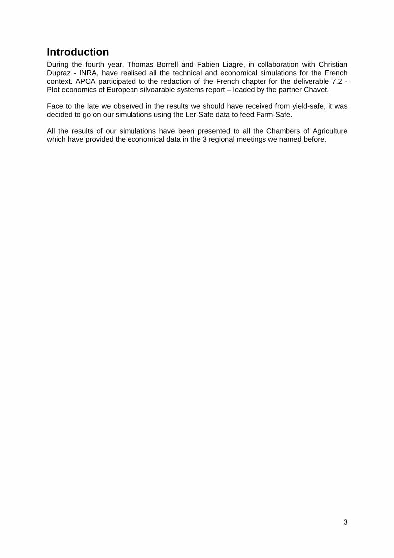
IntroductionDuring the fourth year, Thomas Borrell and Fabien Liagre, in collaboration with ChristianDupraz - INRA, have realised all the technical and economical simulations for the Frenchcontext. APCA participated to the redaction of the French chapter for the deliverable 7.2 -Plot economics of European silvoarable systems report – leaded by the partner Chavet.
Face to the late we observed in the results we should have received from yield-safe, it wasdecided to go on our simulations using the Ler-Safe data to feed Farm-Safe.
All the results of our simulations have been presented to all the Chambers of Agriculturewhich have provided the economical data in the 3 regional meetings we named before.
4
1 The LER approach
LER-biomass and LER-product
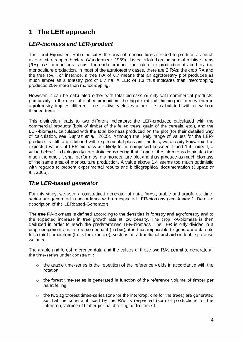
The Land Equivalent Ratio indicates the area of monocultures needed to produce as muchas one intercropped hectare (Vandermeer, 1989). It is calculated as the sum of relative areas(RA), i.e. productions ratios: for each product, the intercrop production divided by themonoculture production. In most of the agroforestry cases, there are 2 RAs: the crop RA andthe tree RA. For instance, a tree RA of 0.7 means that an agroforestry plot produces asmuch timber as a forestry plot of 0,7 ha. A LER of 1.3 thus indicates than intercroppingproduces 30% more than monocropping.
However, it can be calculated either with total biomass or only with commercial products,particularly in the case of timber production: the higher rate of thinning in forestry than inagroforestry implies different tree relative yields whether it is calculated with or withoutthinned trees.
This distinction leads to two different indicators: the LER-products, calculated with thecommercial products (bole of timber of the felled trees, grain of the cereals, etc.), and theLER-biomass, calculated with the total biomass produced on the plot (for their detailed wayof calculation, see Dupraz et al., 2005). Although the likely range of values for the LER-products is still to be defined with experimental plots and models, we already know that theexpected values of LER-biomass are likely to be comprised between 1 and 1.4. Indeed, avalue below 1 is biologically unrealistic considering that if one of the intercrops dominates toomuch the other, it shall perform as in a monoculture plot and thus produce as much biomassof the same area of monoculture production. A value above 1.4 seems too much optimisticwith regards to present experimental results and bibliographical documentation (Dupraz etal., 2005).
The LER-based generator
For this study, we used a constrained generator of data: forest, arable and agroforest time-series are generated in accordance with an expected LER-biomass (see Annex 1: Detaileddescription of the LERbased-Generator).
The tree RA-biomass is defined according to the densities in forestry and agroforestry and tothe expected increase in tree growth rate at low density. The crop RA-biomass is thendeduced in order to reach the predetermined LER-biomass. The LER is only divided in acrop component and a tree component (timber); it is thus impossible to generate data-setsfor a third component (fruits for example), such as for a traditional orchard or double purposewalnuts.
The arable and forest reference data and the values of these two RAs permit to generate allthe time-series under constraint :
o the arable time-series is the repetition of the reference yields in accordance with therotation;
o the forest time-series is generated in function of the reference volume of timber perha at felling;
o the two agroforest times-series (one for the intercrop, one for the trees) are generatedso that the constraint fixed by the RAs is respected (sum of productions for theintercrop, volume of timber per ha at felling for the trees).
5
Amongst the hypothesis made in this generator, we assume that :
o the agroforest trees are felled at the same time as the forest trees, but their highergrowth induces bigger individual pieces of timber; In any case, the unit volume inagroforestry doesn’t exceed 20 % of the forestry volume one.
o there is no difference in the partition of biomass for the intercrop and a classicalarable crop: the crop RA-products is thus equal to the crop RA-biomass, which shallboth be called “crop RA”;
o the intercrops cannot offer higher yields than the arable crops without any tree(consequently the value of the crop RA cannot be superior to the maximumintercropping area: 1 – the proportion of area occupied by the tree strips); we madetherefore the hypothesis that the trees don’t affect positively the crop yield whichcould be discuss on a long term period (soil erosion and fertility, wind effect, etc.).
o the width of the intercropped alley can be reduced by successive steps when theyield decreases (less productive areas are given up), in order to preserveeconomically acceptable yields as long as possible. When it cannot be reducedanymore (at a minimum width), the intercrop is suppressed when it is no moreprofitable (profitability threshold yield).
A wise hypothesis for the agroforest tree growth
In most of the cases, agroforest designs are at lower density than forest designs. As aconsequence, trees grow quicker. We assume that the growth rate increases when thedensity decreases, until to reach a critical final density where the genetic potential is fullyexpressed. Below this density, we assume that trees don’t grow more, even if they arecompletely isolated.
At this critical density, we assume that trees grow at a rate driven by a coefficient: theindividual tree timber volume growth acceleration in low density AF conditions, or TreeGrowth Acceleration (TGA). At critical density, the volume of an agroforest individual piece oftimber at felling, VAF, is thus calculated as:
VmaxAF =TGA x VF
where VF = volume of a forest individual piece of timber at felling (in the forestry reference data which is used).
VmaxAF is thus the maximum volume of an individual piece of timber.
Unfortunately, the critical densities and the likely range of values for TGA are not welldocumented. Thus these parameters had to be fixed by expert knowledge.
In order to realise wise simulations, we assumed a quite low value of TGA: 1,2 for the threespecies (Table I).
VF is the volume of timber of an individual forest tree. TGA is individual Tree timber volume GrowthAcceleration in agroforestry at densities lower or equal to the critical density. The critical density is the highestdensity at which the maximum volume of an individual piece of timber is reached. VmaxAF is the maximum timbervolume of an agroforest tree, reached at densities lower or equal to the critical density.
Table I: reference values in forestry and values of TGA, the critical density and VmaxAF for eachof three tree species
Nevertheless, some unpublished experimental results are in favour of higher values for TGA:at M. Jollet’s farm (Les Eduts, Charentes Maritimes, France), INRA’s measurements of theforest and agroforest trees at the middle of the revolution indicate a TGA of 2 for blackwalnuts, at 80 trees/ha (Gavaland, pers. com.). But another thinning will soon accelerate thegrowth of the forest trees, and then this estimated TGA is likely to decrease.
There is thus an important difference between our hypothesis and what we could expect(Figure 1).
0,5
1
1,5
2
0 20 40 60 80 100Final density (trees/ha)
indi
vidu
al p
iece
of t
imbe
r (m
3/ tr
ee)
with TGA = 2
with TGA = 1,2
Figure 1: Volume of the individual walnut timber volume in function of the final density and ofthe value of TGA.
As an economic consequence of such a wise hypothesis, the volume of timber at felling isless important, thus the revenue of the tree component might be under-estimated.
7
Maximum expectable LER in function of species and final density
As the production of agroforest timber is determined in accordance with the densities, thecritical density and TGA, the tree RA-products and the tree RA-biomass are fixed: it isimpossible to tune them without modifying one of these previous parameters. Then the rangeof variation of the LER (biomass or products) corresponds to the crop RA:
As a LER-biomass inferior to 1 is biologically unrealistic, the minimum value of thecrop RA is equal to 1 – tree RA-biomass.
As we assume lower or equal yields, the maximum value of the crop RA must beinferior or equal to the maximum intercropping area. In our optimistic assumptions, athighest densities (tree lines every 10 m), we assumed a crop RY at ¾ of themaximum intercropping area.
A likely value would be the mean of these two extreme values.
As the proportion of land required by the trees strips rises with the density, the maximumcrop RA decreases when the density gets higher. A first conclusion is that we obtainacceptable RA with densities which correspond to distances between the tree lines includedbetween 24 to 40 m.
0,2
0,3
0,4
0,5
0,6
0,7
0,8
0,9
1
1,1
0 20 40 60 80 100 120 140Distance between the trees lines (m)
LER maxLER-optimistLER-mediumLER-pessimist
No tree
Figure 2: Range of values of the crop RA with walnut, wild cherry and poplar, according thedistance of the tree lines and depending on how optimistic the dynamic of the LER is.
In forestry, the realisation of many thinnings means that a lot of biomass is synthesised inaddition of the trees which shall be conserved until the last fall. As we assume that thevolume of the agroforest trees is maximum 20% bigger than the one of the forest trees, theproduction of woody biomass is small compared to the one of a forestry plot. Thus the ratioof woody biomass, i.e. the tree RA-biomass, is low. At low density, even an optimistic valueof the crop RA is insufficient to compensate such a low tree RA. Consequently, high LER-biomass cannot be reached for all densities, in particular for species with a high rate ofthinning in forestry such as wild cherry (Figure 3).
8
However, very satisfactory LER-products can be reached even with these species.
0,6
0,8
1
1,2
1,4
1,6
0 20 40 60 80 100 120 140Tree final density (trees/ha)
LER
- Pr
oduc
ts
Optimist Crop RA
Medium Crop RA
Pessimist Crop RA
Figure 3: Expectable LER-products for walnut, cherry and poplar, depending on how optimisticthe dynamic of the intercrop is
Impact of the TGA on the LER results
In our simulations, we used a TGA of 1.20. We were cautious in our predictions if weconsider some experimental plots (such in Restinclières in France) or private site (Farm ofClaude Jollet in Charente Maritime) where we observed some TGA which reach 2. If we hadtaken this value of 2, the tree RA would have increased between 15 to 30 % in comparisonwith what we obtained with 1.20.
y = 0,4191x + 0,1123R2 = 0,9995
y = 0,2745x + 0,0955R2 = 0,9987
y = 0,2655x + 0,0018R2 = 0,9989
y = 0,1773x + 0,005R2 = 0,9965
0
0,1
0,2
0,3
0,4
0,5
0,6
0,7
0,8
0,9
1
0,8 1 1,2 1,4 1,6 1,8 2 2,2
Tree Growth Acceleration
TRE
E R
A
120 trees/ha - products
120 trees/ha - biomass
50 trees/ha - products
50 trees/ha - biomass
Figure 4: Influence of the Tree Growth Acceleration on the tree RA (biomass and products),according to the tree density.
9
2 Data references and main hypothesis
The forestry references
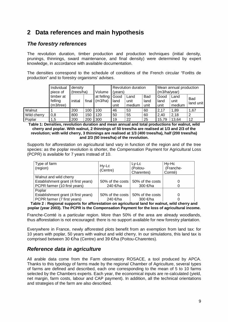
The revolution duration, timber production and production techniques (initial density,prunings, thinnings, sward maintenance, and final density) were determined by expertknowledge, in accordance with available documentation.
The densities correspond to the schedule of conditions of the French circular “Forêts deproduction” and to forestry organisms’ advises.
Table 1: Densities, revolution duration and mean annual and total productions for walnut, wildcherry and poplar. With walnut, 2 thinnings of 50 trees/ha are realised at 1/3 and 2/3 of the
revolution; with wild cherry, 3 thinnings are realised at 1/3 (400 trees/ha), half (200 trees/ha)and 2/3 (50 trees/ha) of the revolution.
Supports for afforestation on agricultural land vary in function of the region and of the treespecies: as the poplar revolution is shorter, the Compensation Payment for Agricultural Loss(PCPR) is available for 7 years instead of 10.
Type of farm(region) Hy-Lc
(Centre)
Ly-Lc(Poitou-Charentes)
Hy-Hc (Franche-Comté)
Walnut and wild cherryEstablishment grant (4 first years) 50% of the costs 50% of the costs 0PCPR farmer (10 first years) 240 €/ha 300 €/ha 0PoplarEstablishment grant (4 first years) 50% of the costs 50% of the costs 0PCPR farmer (7 first years) 240 €/ha 300 €/ha 0
Table 2 : Regional supports for afforestation on agricultural land for walnut, wild cherry andpoplar (year 2003). The PCPR is the Compensation Payment for the loss of agricultural income.
Franche-Comté is a particular region. More than 50% of the area are already woodlands,thus afforestation is not encouraged: there is no support available for new forestry plantation.
Everywhere in France, newly afforested plots benefit from an exemption from land tax: for10 years with poplar, 50 years with walnut and wild cherry. In our simulations, this land tax iscomprised between 30 €/ha (Centre) and 39 €/ha (Poitou-Charentes).
Reference data in agriculture
All arable data come from the Farm observatory ROSACE, a tool produced by APCA.Thanks to this typology of farms made by the regional Chamber of Agriculture, several typesof farms are defined and described, each one corresponding to the mean of 5 to 10 farmsselected by the Chambers experts. Each year, the economical inputs are re-calculated (yield,net margin, farm costs, labour and CAP payment). In addition, all the technical orientationsand strategies of the farm are also described.
10
We selected 3 types of farm, which we shall now designate with 4 initials:
Hy-Lc: High yields and Low fixed costs
Hy-Hc: High yields but High fixed costs
Ly-Lc: Low yields and Low fixed costs
For each of them, the ROSACE typology indicates:
The cropping area of the farm, distinguishing tenant farming and property;
The crop rotation in function of the quality of the soil (up to 3 Land Units: best,medium, worst);
The mean yields, attributed to the medium Land Unit (for the best and worst LandUnits, we respectively assumed an increase and a decrease of 10% of the meanyields);
The variable costs, assignable fixed costs and fixed costs and labour.
The prices of the products and sub-products (straws of the wheat) and the CAPpayments of the farm Single Farm Payment, SFP).
To elaborate the selection of each type of farms, various partners from the Chambers ofAgriculture have participated: Camille Laborie, who is in charge of ROSACE in APCA, Anne-Marie Meudre (Franche Comté), Catherine Micheluzzi (Poitou-Charentes) and Benoît Tassin(Centre).
Table 3 : Main economic data and total net margin (€/farm) for every type of farm. Rotation (a)corresponds to the best land units, rotation (b) to the worst. Set aside is realised on 10% of the
total farm area.
The Net Margin is equal to the Gross Margin minus the fixed assignable costs (land tax andmachinery costs). The Total Net Margin is equal to the Net Margin minus the fixed costs (rentof land, amortisation and maintenance of the buildings, social contributions, banking costs).Labour costs are not taken into account.
The profitability threshold yield
With the development of the trees, the crop yield decreases progressively. Below a certainlevel, the crop is not more profitable, above al near the tree area. For each crop of the threetypes of farm, the threshold yield was first determined according to the price of the product,the CAP payment and the variable costs, assignable fixed costs and a part of the fixedcosts1. As the results, in proportion of the mean yield of each crop, were roughly the same inthe three farms, we fixed this proportion in order to facilitate the extrapolation to other typesof farm.
1 If the crop is abandoned on a part of the cropping area, we assume that the fixed costs shoulddecrease a little; thus they must be taken into account in the calculation of this threshold yield.
Table 4: Profitability threshold yield in proportion of the mean yield in the farm and example forthe farm Hy-Hc
The threshold yield is the same in every farm, whatever the land unit is. Thus it shall bereached more quickly in the worst land unit than in the best land unit.
Main management features of the agroforestry systems
For each type of farm, we simulated the introduction of 2 agroforestry designs in the 3 landunits (best, medium, and worst):
Plantation at 50 trees/ha, on 40 m spaced tree-lines;
Plantation at 120 trees/ha, on 22 m spaced tree-lines.
The tree strip is 2 m wide. The width of the intercropped alley is respectively of 38 m and 20m, thus the maximum crop area represents 95% of the initial area at 50 trees/ha and 91% at113 trees/ha.
With walnut and wild cherry, an early thinning is realised when the timber volume reaches0,1 m3 (around the years 10-13), therefore the final densities are different from the poplars’one (see Table 5).
Table 5: Initial and final densities, volume of an individual piece of timber and production inforestry and in the simulated agroforestry systems; tree Relative Area (RA)-biomass and tree
RA-products
The crops Relative Areas (RA) have been fixed for 3 hypothesis: optimistic, probable andpessimistic.
The pessimistic hypothesis means that the LER-biomass is equal to 1. Therefore, the cropRA is equal to: (1 – tree RA-biomass).
The optimistic crop RA is determined according to 2 constraints:
The crop RA must be inferior to the maximum intercropping area
13
We also assumed to fix a ceiling for the LER-biomass of 1.4. Thus the crop RA isequal to: (1.4 – tree RA-biomass). This ceiling of 1.4 was reached with walnut andpoplar at 120 trees/ha, so the crop RA seems quite low with regards to the maximumintercropping area.
We assumed a probable crop RA as the arithmetic average of the 2 previous values(pessimistic and optimistic) (see Table 6 and Table 7).
Table 6: Crop RA in function of the tree species, density and optimism level. Bold values arethose which depend on the ceiling of 1.4 for the LER-biomass.
Table 7 : LER-biomass and LER-products in function of the tree species, density andhypothesis of optimism for the intercrop bold values are those which depend on the ceiling of
1.4 for the LER-biomass.
Economic hypothesis
CAP paymentsIn agriculture, the crops area benefits from the Single Farm Payment (SFP): it was calculatedon the basis of the historical references of each farm, in accordance with the way Francedecided to implement the new CAP in 2006.
In the basic scenario, we assumed that the intercrops are eligible to the SFP proportionally tothe area of the plot that they occupy. It is the present situation in France. The rightscorresponding to the tree area could be transferable to another eligible area which doesn’tbenefit from a payment right. In our simulations, we did not attribute them to new plots,considering therefore that these rights were lost for the farmer.
Tree grantsIn our basic scenario, agroforest trees benefit from the same establishment payments as theforest trees: 50% of the costs of the 4 first years in Poitou-Charentes and Centre. Itcorresponds to the present situation, permitted by the circular “Forêts de protection” which
14
relies on the line i of the French National Rural Development Programme. However anagroforest plot cannot benefit from neither the PCPR nor the exemption of land tax.
In France, an agro-environmental measure called “agroforest habitats” can be contractedunder certain conditions, but it still faces administrative difficulties and is not available in mostof the departments, thus it was not taken into account in our simulations.
Costs and pricesSome key points have to be underlined:
The cost of sward maintenance is higher in forestry than in agroforestry. In forestry, atthe beginning of the revolution, sward maintenance is realised thanks to two grindingsinstead of one for the maintenance of the tree strip in agroforestry.
The farmer makes all operations himself, except the marking out and plantation of theyoung trees. Both of these operations are charged 15 €/h. The timber pricescorrespond to standing trees, thus neither the harvesting cost is taken into account.
In a cash flow approach, the basic scenario doesn’t include the labour cost for thefarmer. While in a farming management scenario, we consider an hourly cost of 7,62€/h (minimum salary in France). In this last approach, it’s therefore possible toevaluate the efficiency of the farmer labour.
As it seems impossible to anticipate the future evolution of prices and costs, we assumedconstant values. For instance, a rise or a drop of timber value would respectively increase ordecrease the tree revenue.
15
3 Main results
Labour impact for one silvoarable hectare
0
2
4
6
8
10
12
14
16
1 6 11 16 21 26 31 36 41 46année
temps de travail(h/ha/an)
agriculturecultures intercalairesarbres
Case 1: Plantation of 120 trees/ha Case 2: Plantation of 50 trees/ha
Figure 5: Labour evolution in the management of a silvoarable plot during the tree rotation,separating the crop from the tree labour.
An essential condition for adopting agroforestry from the farmers’ point of view is that theydon’t want to devote more time to a new system. If the farmer planted more trees (case 1),he would need 1 to 1.5 days each year to maintain the trees. But in the second half of therotation, the labour decreases progressively due to the fact that trees don’t need morespecial maintenance and that the intercrop activity is reduced. If he plants fewer trees, theimpact during the first years is poor. With the small density, the intercrop activity is longer,because the crop yield is not so affected by the trees. The labour requested in the secondhalf of the rotation is therefore lower but very near from the initial scenario.
Prediction of yield evolution
Crop yield evolutionPredicting the crop yield during the second half of the rotation is a perilous venture. If weknow the behaviour of the intercrop during the first half thanks to experimental measures onexisting plots, we asked the bio-economics model to predict the yield evolution. In oursimulation, as we said, we used the LER-Safe prediction. We made the essential hypothesisthat the LER must be include between 1 and 1.4. This condition helps us to determine apossible range of crop yield evolution, from the pessimist one to the optimist one (see Figure6).
0
2
4
6
8
10
12
14
16
1 6 11 16 21 26 31 36 41 46année
temps de travail(h/ha/an)
agriculturecultures intercalairesarbres
16
0
20
40
60
80
100
0 Time
Cro
p yi
eld
(%)
0
20
40
60
80
100
Intercrop Yield
Pure Crop
Tree HarvestTree plantation
Optimist
Pessimist
Figure 6: Evolution of the relative intercrop yield according to optimist or pessimist view aboutthe tree competition. Case of one ha of wild cherry with an initial density of 120 trees/ha for a
final density of 80 trees/ha.
In this example of a plantation of wild cherry at 80 trees/ha (final density), which means adistance between the trees rows of 25m, the crop yield represent more than 90% during thefirst half of the tree rotation. According to the interaction level, the crop yield varies between30 and 75 % of the pure crop yield of reference the year before harvesting the trees.
The crop yield depends on different parameters:
The parameters due to some initial choices: the crop nature (a sunflower will be moreaffected by the shadow of the adult trees than a cereal), the density of the plantationand the distance between the lines, choice of the land unit (a deeper soil will be moreadapted),...
The parameters depending on the capacity of the farmer: well pruned trees, tree rootmaintenance (root cutting), …
In our economical scenarios, we have tested the different level of interaction.
Tree yield evolutionAs for the crop yield estimation, we put forward the hypothesis of different level of timberproductivity. But for our simulations, we only use one prediction of timber production. Tovalidate our approach, we use a very cautious estimation of production (see Figure 7). Ourresults can therefore be considered as the minimum result we can get from our hypothesis.
17
0
20
40
60
80
100
120
140
5 10 15 20 25 30 35 40 45
Time
Sta
ndin
g vo
lum
e (m
3/ h
a)
0
20
40
60
80
100
120
140Interval
BasicscenarioPureplantation
Optimist
Pessimist
Figure 7: Range of timber volume evolution for an initial plantation of 120 wild cherry. Thefigure indicates of the cautious hypothesis of standing volume we used for our simulations (77
m3 for 80 final trees).
Cash flow impact
To evaluate the impact of the project on the cash flow, we must distinguish first theinvestment cost and then the evolution of the annual cash flow depending of the crop yieldevolution and the possible over cost to crop between the trees in comparison with a purecrop system.
Initial investmentThe poor number of trees to plant in an agroforestry system reduces considerably theinvestment cost if we compare with a current afforestation cost on agricultural land. The treecost is nonetheless higher. The owner will choose a better quality of the trees and will haveto protect each one with a strong protection: each tree has a possible future value anddemands a special attention.
The total cost of a plantation (without subsidy) varies between 500 and 1000 euros/haaccording to the tree specie (the walnut plantation being the most expensive). This costrepresents between 20 to 60 % of the average cost in the case of common land afforestation(see Figure 8).
517 €/ha1 034 €/ha
1 633 €/ha
267 €/ha
469 €/ha
1 518 €/ha
367 €/ha695 €/ha
1 233 €/ha
Walnut
Wild Cherry
Poplar
Afforestation
120 trees/ha
50 trees/ha
Figure 8: Comparison of the investment in agroforestry and forestry scenario, WITHOUTsubsidy.
18
In France, it’s current to get a subsidy of 40 to 70% to cover the investment cost and themaintenance cost of the trees during the 4 first years (except in Franche Comté).
Since 2004, the French Government decided to suspend all economic aids to the landafforestation, excepted for agroforestry. In our simulations, we decided to conserve this aid,to be able to compare between the two options (see Figure 9).
259 €/ha517 €/ha
817 €/ha
134 €/ha
235 €/ha
759 €/ha
184 €/ha
348 €/ha
617 €/ha
Walnut
Wild Cherry
Poplar
Afforestation
120 trees/ha
50 trees/ha
Figure 9: Comparison of the investment in agroforestry and forestry scenario, WITH subsidy.
Cash flow evolution
Evolution of the cash flow at the plot scale
The cash flow evolution will depend of the crop yield evolution and the LER level we haveselected and the final density. For example, in the Figure 10, we’ve illustrated the cashevolution for two different densities but for a medium LER level.
0
10
20
30
40
50
60
70
80
90
100
Time
% A
nnua
l Gro
ss M
argi
n
0
10
20
30
40
50
60
70
80
90
100
Silvoarable Gross Margin
Agricultural Gross Margin
70 to 85 %
30 to 60 %
80 to 90 %
PlantationTrees Harvesting
50 trees/ha
120 trees/ha
Figure 10: Evolution of the annual cash flow for a probable scenario with wild cherry (LER=1.07for a density of 50 trees/ha and 1.15 for a density of 120 trees).
19
Being cautious in our forecast, we notice nonetheless that at half of the rotation, the grossmargin still represent 80 to 90 % of the agricultural gross margin. We must underline that inour simulations, we’ve considered that the crop payment area is reduced progressively bythe tree area. In case of the silvoarable area was eligible in its totality, the impact on the cashwould be sensible, above all in some regions where man get poor crop yield and where thecrop payment is essential in the gross margin calculation (Franche Comté for example).
Let’s also underline the fact that in the INRA experimental plots, the LER reaches more 1.3than 1.15 that we have chosen in our simulation with an initial density of 120 trees/ha.
Influence of the CAP payment policy
Inside the first pillar policy, the situation of the agroforestry plots could be different dependingof each country member. In fact, at a European level, the agroforestry plot could be eligibleto the Compensatory Payment. We compare here the possibility to get the payment on thewhole area (Request of the Safe consortium) or only on the intercrop area (French situation).
The impact of the eligibility given to the whole surface on the profitability is not so important.In all our simulations, the profitability increases by 3% in the best option for agroforestry. Theimpact is more at a cash flow level, when the crop gross margin is low. That’s typically thecase for the farms where:
The crop component is lower than the payment component in the gross margincalculation (Mediterranean area or farm with high cost of production)
The yield is decreasing faster in the silvoarable scenario (high density of plantation orstrong impact of the trees on the crop RA) (see Figure 11)
0%
20%
40%
60%
80%
100%
2% 12% 22% 32% 42% 52% 62% 72% 82% 92%
Time (Tree rotation)
% o
f the
Ara
ble
Gro
ss M
argi
n
agriculturePayment on intercrop area - 50 trees/haPayment 100% - 50 trees/haPayment on intercrop area - 120 trees/haPayment 100% - 120 trees/ha
Figure 11: Influence of the different CAP payment policies in agroforestry on the annual cashflow evolution.
Evolution of the cash flow at the farm scale
At the farm scale, one of the first questions of the farmer is about the importance of the areato plant. Does he have to plant on a big area? In several plots or in a single plot? There is noonly one answer. According to the strategy of the farmer, a large range of scenarios isavailable. The choice will depend to the cash flow context and to know if the farmer cansupport a strong investment or not, and above all if he aims to decrease progressively his
20
crop activity or not. The labour availability is also a strong parameter to decide which area toplant. According to our simulation and experimental experience, we often recommend notplanting more than 10 % of the cropping area. In that case, the impact on the farm grossmargin is less than 3 % in average on the first half of the tree rotation. A gradual plantationwill allow a reduction of the cash flow impact (see Figure 12).
50
75
100
125
150
175
0% 20% 40% 60% 80% 100% 120%% of the tree rotation
% o
f Far
m G
ross
Mar
gin
with
out A
F
Farm with 8% silvoarable area
Farm with 100 % of cropping area
435 %
50
75
100
125
150
175
0% 20% 40% 60% 80% 100% 120%% of the first tree rotation
% o
f Far
m G
ross
Mar
gin
with
out A
F Farm with 8% silvoarable area
Farm with 100 % of cropping area
178% 180% 191% 183%
a. Case of a single plantation b. Case of a gradual plantation
Figure 12: Comparison of the cash flow evolution when the farmer plants 8 % of his croppingarea (50/50 Walnut/Wild cherry). We compare the option where the farmer would plant thesilvoarable area in once time or if he decides to plant 2 % every 5 years during 20 years.
A gradual plantation will also allow a soft distribution of the timber income in the time fromthe moment where the owner begins to harvest the first mature trees (case b). From thismoment, the timber income is regular. In our example, he can harvest the trees every 5years. In this context, the farm gross margin increase by 15 %. According to the importanceof the plantation and of the species he planted, a farmer could increase his farm incomebetween 10 to 100%. Of course, it can suppose a long term to wait for the farmer before thefirst tree harvest…
Profitability of a silvoarable investment
Comparing a silvoarable scenario with agricultural scenarioFor our simulations, we have selected 3 kinds of farms:
Farm with good crop yields and few fixed costs.
Farm with medium crop yields with few fixed costs.
Farm with medium crop yields and high fixed costs.
For each farm, corresponding to each region of the LTS of the WP8, we have run differentscenarios according to:
the tree density: 120 versus 50 for the initial density which corresponds to a finaldensity of 80/40.
the LER level: optimist, probable and pessimist
the land unit: good/medium
the 3 tree species: poplar, walnut and wild cherry
21
108 scenarios have been run in total (36 scenarios / LTS). The Figure 13 shows a synthesisof the Agricultural Values for all these scenarios we have calculated for each specieaccording to the level of LER.
0%
20%
40%
60%
80%
100%
optim
ist
proba
ble
pess
imist
optim
ist
proba
ble
pess
imist
optim
ist
proba
ble
pess
imist
Scenario for intercrop productivity
% o
f rea
lised
sim
ulat
ions
> 1,35
1,20 - 1,35
1,05 - 1,20
0,95 - 1,04
< 0,95
Walnut Wild Cherry Poplar
AgriculturalValue Index
Figure 13: Profitability of the silvoarable scenarios according to the tree specie and the LERlevel.
A first interesting result is that the silvoarable scenarios are at least as profitable as theagricultural scenario.
Walnut timber is actually the most expensive timber on the market. For a same duration ofrotation, the best results have been logically obtained with the walnut than the wild cherry.The period of harvesting time is a key parameter in the profitability calculation (see Figure14).
0 , 0 0
0 , 2 0
0 , 4 0
0 , 6 0
0 , 8 0
1 , 0 0
1 , 2 0
1 , 4 0
1 , 6 0
1 , 8 0
2 , 0 0
T r è s b i e nf o r m é
( 4 0 a n s )
B i e n f o r m é( 5 0 a n s )
M a l f o r m é( 6 0 a n s )
Very well pruned Well pruned Badly pruned
40 years 50 years 60 years
0 , 0 0
0 , 2 0
0 , 4 0
0 , 6 0
0 , 8 0
1 , 0 0
1 , 2 0
1 , 4 0
1 , 6 0
1 , 8 0
2 , 0 0
T r è s b i e nf o r m é
( 4 0 a n s )
B i e n f o r m é( 5 0 a n s )
M a l f o r m é( 6 0 a n s )
Very well pruned Well pruned Badly pruned
40 years 50 years 60 years
Figure 14: Influence of the maintenance quality on the profitability.
22
A late in the pruning dates can put the harvesting date back by 10 or 20 years, above all forsome sensitive specie such as the hybrid walnut. In this example, a late of 20 years means areduction of 60% of the profitability in comparison of the agricultural profitability.
Influence of the TGA on the Agricultural ValueThe value of the Tree Growth Acceleration has a strong impact on the profitability of thesilvoarable scenarios. This impact is stronger for the scenario with higher densities ofplantation. In the following figure, we noticed that the scenario with a density of 120 ha reactmuch quicker than a scenario with 50 trees.
Again, in our simulations, we used a TGA of 1,20 which could be considered as a pessimistapproach with what we observe in the reality. For example, in the Jollet's case, theagricultural value would have been increased by 10 to 15 % (see Figure 15).
0,90
0,95
1,00
1,05
1,10
0,8 1 1,2 1,4 1,6 1,8 2Tree Growth Acceleration
Indi
ce o
f Agr
icul
tura
l Val
ue
120 wild cherry/ha
50 wild cherry/ha
Hypothesis simulation
Jollet TGA
Figure 15: Influence of the TGA on the Agricultural Value
Which density to plant to get the best profitability?A common question from the farmers is about the number of trees to plant. The farmers oftenwant to maintain a correct crop yield during the whole rotation but trying in the same time toget the best investment for timber. Other decides to plant more trees with the aim todecrease the agricultural activity, even till to suppress the intercrop. We didn’t take this casein this study.
For each specie, Walnut, Wild cherry and Poplar, according to our production hypothesis, wesimulated the impact of the density to the LER but also to the Agricultural Value (see Figure16).
23
0,6
0,8
1
1,2
1,4
1,6
0 20 40 60 80 100 120 140WILD CHERRY - Finale Density (trees/ha)
LER_optimist
LER_medium
LER_pessimist
Val-agri_optimist
Val-agri_medium
Val-agri_pessimist
0,6
0,8
1
1,2
1,4
1,6
0 20 40 60 80 100
WALNUT - Final Density (trees/ha)
LER_optimist
LER_medium
LER_pessimist
Val-agri_optimist
Val-agri_medium
Val-agri_pessimist
0,4
0,6
0,8
1
1,2
1,4
1,6
0 50 100 150 200
POPLAR - Final density (trees/ha)
LER_optimist
LER_medium
LER_pessimist
Val-agri_optimist
Val-agri_medium
Val-agri_pessimist
Figure 16: Influence of the tree density on the LER value and the Agricultural value for wildcherry, walnut and poplar.
24
We observe that for each specie, the best density to get the optimum LER is higher than thebest density to get the optimum Agricultural Value. For the species with a poor Tree RA(Walnut and wild cherry), the range of density are similar (see Table 8). The best densitywould vary between 80 to 120 trees/ha to get the highest LER, while the farmer will get thebest profitability with a density included between 60 and 90 trees/ha. Of course, with a higherTGA, this range would increase.
Result Wild Cherry Walnut Poplar
LER 80 - 120 80 - 120 130 - 200
Agricultural Value 60 - 90 60 - 90 100 - 130
Table 8: Range of density to get the optimum LER and Agricultural Value results for eachspecie (trees/ha – final density).
For the poplar, the optimum densities are higher than for the 2 others species. This result isdue to the fact that the biomass produced by the silvoarable poplar is similar to the biomassproduced by the forestry poplar. The Tree RA is therefore higher for a given densitycompared to other species which demand more important fellings.
What could influence these results? As we already said, the TGA level could stronglyinfluence these results, giving priority to higher densities. The policy schedule and the pricelevel of the crop and tree component will be therefore the most important parameters. In thecase of the walnut, the choice of a density of 75 trees/ha is a wise option. Below, the farmdoesn’t want to take any risk at a long term period, above he bets more on the trees.
Comparing a silvoarable scenario with a forestry scenarioWe compare also the case where the farmer was hesitating between a forestry investmentrather than a silvoarable investment from a profitability point of view (see Figure 17).
0,89
1,21
0,48
1,04
1,55
1,00
0,00
0,50
1,00
1,50
of a silvoarable scenario
of a pure plantation scenario
Agricultural Value Index
Poplar Walnut Wild Cherry
Figure 17: Comparison of the profitability of the silvoarable and afforestation scenario with theagricultural scenario. Silvoarable plantation of 120 wild cherry by ha characterized by a LER of
1,15.
In this example, we explore the case of a probable LER of 1.15 in the silvoarable option. Inalmost all our simulations, the silvoarable options are more profitable than the forestry option.
25
The forestry option may be more profitable in the case where the crop margin is very poor,above all if it’s possible to plant some valuable species such as walnut for example.
It’s also interesting to notice that for the poplar, the silvoarable option could be a possibility tostimulate the poplar market. In France, the poplar area is currently decreasing because ofthe price fall of the timber (less than 45 €/m3). Agroforestry could therefore be a possiblestrategy to reduce the market risks.
Property holdings evaluation in agroforestryAccording to his age, a land owner who plants trees, will not necessary benefit from theharvest… But, as a farmer told us, a farmer has three possibilities of income: the sale of hisproducts, the stock variation and the possibility to make a capital gain. In this last option, asilvoarable plot is a capital which could be evaluated if necessary (inheritance, expropriation,etc). The land evaluation in agroforestry is the combination of the agricultural land evaluationand the future value of the trees (see Figure 18).
0 €
2 000 €
4 000 €
6 000 €
8 000 €
10 000 €
12 000 €
14 000 €
16 000 €
10 20 30 40
Age of the trees (years)
Euro
s by
ha
Agriculture agroforestry
with commercial valueNo commercial value
Figure 18: Evolution of the monetary value of the silvoarable land according to the age of thetrees. In agroforestry, this value is the sum of the agricultural value plus the timber futurevalue. If the young trees could have a future value, for example at 10 years old, they don’tnecessary have a commercial value in the sense that the landowner can not expect some
income if he cut them.
In this example of a wild cherry plantation, the capital evaluation may represent betweentwice and four time the agricultural land value according to the age of the trees. In the caseof a walnut plantation, it may represent till 7 times this value 10 years before the treeharvesting.
26
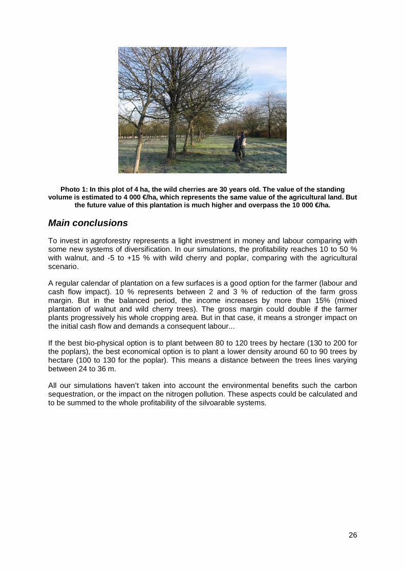
Photo 1: In this plot of 4 ha, the wild cherries are 30 years old. The value of the standingvolume is estimated to 4 000 €/ha, which represents the same value of the agricultural land. But
the future value of this plantation is much higher and overpass the 10 000 €/ha.
Main conclusions
To invest in agroforestry represents a light investment in money and labour comparing withsome new systems of diversification. In our simulations, the profitability reaches 10 to 50 %with walnut, and -5 to +15 % with wild cherry and poplar, comparing with the agriculturalscenario.
A regular calendar of plantation on a few surfaces is a good option for the farmer (labour andcash flow impact). 10 % represents between 2 and 3 % of reduction of the farm grossmargin. But in the balanced period, the income increases by more than 15% (mixedplantation of walnut and wild cherry trees). The gross margin could double if the farmerplants progressively his whole cropping area. But in that case, it means a stronger impact onthe initial cash flow and demands a consequent labour...
If the best bio-physical option is to plant between 80 to 120 trees by hectare (130 to 200 forthe poplars), the best economical option is to plant a lower density around 60 to 90 trees byhectare (100 to 130 for the poplar). This means a distance between the trees lines varyingbetween 24 to 36 m.
All our simulations haven’t taken into account the environmental benefits such the carbonsequestration, or the impact on the nitrogen pollution. These aspects could be calculated andto be summed to the whole profitability of the silvoarable systems.
27
4 BibliographyBorrell, T. (2004) De l’importance des interactions arbres-cultures sur les performances
économiques de l’agroforesterie tempérée. Mémoire de Diplôme d’AgronomieApprofondie, ENSAM-INRA, Montpellier. 98 p + annexes
Boulet-Gercourt, B. (1997) Le merisier. IDF, 2ème édition. 128 pp.
Coulon F, Dupraz C., Liagre F., Pointereau P. (2000) Etude des pratiques agroforestièresassociant des arbres fruitiers de haute tige à des cultures et pâtures, Rapport auministère de l’environnement, 199 p, Solagro/INRA, Fr
CRPF (1997) Boiser une Terre Agricole. 28 pp.
Dupraz C., Lagacherie M., Liagre F., Boutland A., (1995). Perspectives de diversification desexploitations agricoles de la région Midi-Pyrénées par l’agroforesterie. Rapport de find’étude commandité par le Conseil Régional Midi-Pyrénées, Inra-lepse éditeur,Montpellier, 253 pp.
Dupraz C., Lagacherie M., Liagre F., Cabannes B., (1996). Des systèmes agroforestiers pourle Languedoc-Roussillon. Impact sur les exploitations agricoles et aspectsenvironnementaux. Inra-Lepse éditeur, Montpellier, 418 pp.
Dupraz, C., Liagre, F. & Borrell, T. (2005) The Land Equivalent Ratio of a silvoarableagroforestry system. In preparation.
Graves, A.R., Burgess, P.J., Liagre, F., Dupraz, C. & Terreaux, J.-P. (in preparation) Thedevelopmentof an economic model of arable, agroforestry and forestry systems. To bepublished soon in Agroforestry Systems.
IDF (1997) Les noyer à bois. 3ème édition, Février 1997. 132 pp.
Liagre F., (1993). Les pratiques de cultures intercalaires dans la noyeraie fruitière duDauphiné. Mémoire de Mastère en Sciences Forestières, ENGREF, Montpellier, 80 pp
Segouin O., Valadon A., (1997) Enquête sur les boisements récents de peupliers en Lot-et-Garonne, Analyse de pratiques agroforestières ; les cultures intercalaires. Cemagref,Nogent-sur Vernisson, 45 pp.
Souleres, G. (1992) les milieux de la populiculture, IDF, 310 pp.
Terreaux, J.-P. & Chavet, M. (2002) Problèmes économiques liés à l’agroforesterie :éléments qualitatifs et quantitatifs. Silvoarable Agroforestry For Europe (SAFE) ;Cabinet Michel Chavet, Paris – UMR Lameta, Montpellier.
Vandermeer, J. (1989) The Ecology of Intercropping, Cambridge University Press, 225 pp.
28
5 Annex
Annex 1: Detailed description of the LERbased-Generator
Principle
Farm-SAFE does not have any biophysical module, the time-series must be generatedindependently: pure crop and intercrop yields, timber production in forestry and agroforestry.We used a generator constrained by the LER-biomass: depending on a previously fixedvalue and on a quite low number of parameters, these times-series are produced. Thestarting and final points are known, the evolution between them is drawn thanks to a logisticequation.
A key characteristic is that the climatic variability is not taken into account. It would havenecessitate to define the impact of variables (temperature, water, light, etc...) which are notimplicated in this type of constrained prediction. Nevertheless, we assume that except in veryparticular cases, this variability does not have any impact on the economic results: on awhole revolution (20 to 60 years), “bad weather” years are compensated by “good weather”ones, as we are not interested in year-by-year results but final profitability and globalevolution of financial results. Because of discounting, climate would only have a strong effectif “bad weather” years were concentrated in a specific part of the revolution, which is veryunlikely to happen.
Notations
We use the words “forestry” and “forest trees” for all types of pure trees plantation, evenwhen the initial density is very low, such as for walnut.
A distinction is made, in forestry and agroforestry, between the trees which are cut atthinnings and the trees which are maintained until last felling: the firsts are called “thinnedtrees”, the others “felled trees”.
We call “timber” the bole of the tree, which has the highest commercial value. The sameword is used for the thinned trees, even if the bole is often too small to be sold as goodtimber.
VF is the individual forest tree timber volume at forestry reference density.
VAF is the individual agroforest tree timber volume, depending on the density.
VmaxAF is the maximum individual agroforest tree timber volume.
Parameters
Parameters per tree species
- DC, the critical agroforestry density, i.e. the density at which the tree growthpotential is attained: the individual agroforest tree timber volume is equal to VmaxAF,the trees cannot be bigger, even at lower densities.
- TGA, the coefficient of individual Tree timber volume Growth Acceleration inlow density AF conditions, or Tree Growth Acceleration; e.g. 1,2 indicates that theindividual agroforest tree timber volume at a lower or equal density than DC will be20 % bigger than the one of a forest tree, due to the positive impact of both low
29
density and intercropping (exceeds of nitrogen, less competition than the perennialvegetation classically established between forest trees, etc…).
- Timber To Biomass in forestry, e.g. the timber contribution to the total biomassof a young forest tree (TTByoung-F) and of a felled forest tree (TTBfell-F);
- Timber To Biomass of a felled agroforest tree (TTBfell-AF);
- maximum value for the forestry ratio: biomass of all the thinned trees/biomassof all the felled trees;
- individual tree timber volume of the agroforest tree at thinning.
Parameters of the logistic curves
- curvature and inflexion for the individual forest tree timber volume, for theindividual agroforest tree timber volume;
- curvature and inflexion for the height of the forest trees, of the agroforesttrees;
- curvature for the intercrop yields.
Parameters used only as Farm-SAFE entries2
- final tree height (same in forestry and agroforestry);
- maximum bole height (same in forestry and agroforestry);
- fixed value of the ratio: firewood volume/timber volume in forestry, inagroforestry.
Entries
- arable rotation, reference yield and threshold yield for profitability for everycrop;
- tree species, revolution duration (60 years maximum);
- forestry: reference production, initial density, years of thinnings (maximum 5)and numbers of thinned trees;
- agroforestry: initial density, number of trees cut in the unique thinning, plotdesign (distance between tree lines, initial width of the intercropped alley, width ofthe intercropped alley reduction step);
- LER-biomass aimed.
2 These three parameters are not used in the generation of tree production data-sets (timber), but theyare needed as entries for Farm-SAFE (tree height and production of firewood).
30
The generation of data-sets
The first step is the generation of the time-series of the monocropping systems:
The time-series of pure agricultural yields are produced simply by repeating the referenceyields as many times as necessary to last the duration of the revolution.
The time series of the timber production of the felled trees are generated with the followinglogistic equation:
Yt = finalcourbure
lexion
finalinitial Y
Tt
YY
inf1
where Yt is the value of Y at year ;
Y initial and Y final are the initial and final values of Y;
T inflexion is the inflexion date (end of linear growth).
Y initial is equal to zero and Y final to any value, as the curve is then distended in order to gothrough a point {X’;Y’}: X’ is the date of fell of the trees and Y’ is the reference production (inm3/ha of timber at felling).
For forestry, 3 other time series are generated :
- The timber production of the thinned trees3, as it is considered that they canbe smaller than the felled trees. The same logistic equation is used, with an Y’calculated in function of 2 constraints:
(i) thinned tree timber volume felled tree timber volume.
(ii) the parameter “maximum value for the ratio: biomass of all thethinned trees/biomass of all the felled trees”
- The biomass of both the felled and the thinned trees, thanks to the ratioTimber To Biomass. We assume that if TTBF may vary with time t, it is a linearvariation:
FyoungFyoungFfell
F TTBtTTTBTTBtTTB
where T is the revolution duration.
The biomass of the felled trees and of the thinned trees is thus calculated by dividing theirrespective timber time series by TTBF(t).
3 There is only one time series for all the thinnings: late-thinned trees have the same rate of growth asearly-thinned trees.
31
The Relative Areas calculated in function of the Tree Growth Acceleration:
The coefficient of individual Tree timber volume Growth Acceleration in low density AFconditions, or Tree Growth Acceleration (TGA), permits the calculation of the agroforest treetimber volume:
- At D DC, VAF = VmaxAF
- At D = DF, VAF = VF
- D > DF is not possible
- At DC < D < DF, VAF =CF
FAFF
CF
AFFF DD
VVDDDVVDV maxmax
Where: D, DC and DF are the actual density, the critical density and the forestdensity
VAF, VF and VmaxAF are the actual agroforest tree timber volume, the foresttree timber volume and the maximum agroforest tree timber volume, withVmaxAF = TGA x VF
On the basis of the final densities in forestry and agroforestry, the forestry RA- products canthen be deduced.
With TTBfell-AF, we easily know the agroforest trees biomass at f elling.
With regards to the low initial density in agroforestry, we assume that the thinned trees growas well as the felled trees: the thinning is early enough to avoid a strong effect of competition,thus the individual thinned tree timber volume is the same as the one of a felled tree at thattime. And as the number of thinned trees is low and the thinning quite early, the volume ofthinned biomass is poor enough to permit us to consider a fixed TTBAF in time. Thus thevolume of thinned biomass in agroforestry is calculated by dividing the thinned timberproduction by TTBfell-AF.
The forestry RA-biomass can then be calculated.
The arable RA-biomass is deduced in function of the aimed LER-biomass. It is equal to thearable RA-products, as we assume that the proportion of grain in the biomass of the crop isthe same in agriculture and in agroforestry.
The generation of the agroforestry data-sets:
The agroforestry timber time-series are generated with the same logistic equation: Y’ is thenthe forestry reference production multiplied by the forestry RA-products.
Until the thinning, the volume of timber of the thinned trees is taken into account simply byadding the equivalent number of trees with the same individual tree timber volume.
The intercrop time-series are also generated with this logistic equation, with an Yfinal equalto 0: one time-series per crop of the rotation (maize, wheat, oilseed, etc...). For each crop,the curve is adjusted in function of the threshold yield and the width of the intercropped alleyreduction step: as the yield per total ha decreases with time due to tree growth andincreasing light competition, we assume that the cropped area is reduced by successivesteps (see Figure 19). A reduction of the width of the intercropped alley happens every time
32
the yield per cropped ha passes under an economically defined threshold. The last reductioncorresponds to the suppression of the intercrop.
Figure 19: chronological schema of the intercropped area in the alley in function of treegrowth.
The width of the intercropped strip (w) is reduced at t1 and t2 in order to increase the mean yield percropped ha. Its next reduction at t3 corresponds to the suppression of the intercrop. In the generator, upto 6 reductions can be made.
The intercrop curves are adjusted by modifying their inflexion date so that the sum of theintercrop productions is equal to the crop reference yield multiplied by the arable RA-products.
The intercrop time-series are then mixed according to the arable rotation to obtain a singletime-series.
The same tree height curve time series in forestry and agroforestry
A last time-series is generated for both forest and agroforest trees : their height growth. It isnot used in the timber volume calculation, but this time-series is needed in Farm-SAFE for its“autoprune” function.
We use the Boltzmann logistic equation :
0)(inf
1tfinal
curvatureTt
finalinitialt YY
e
YYYlexion
w
33
As for the timber time-series, Y initial is equal to zero and Y final to any value, as the curve isdistended in order to go through a point {X’;Y’} : X’ is the date of fell of the trees and Y’ is theaimed height.
34
Annex 2: Labour, revenues and costs in the 3 types of farms
Crop Annual labour(h/ha)
Price
(€/t)
Single FarmPayment
(€/ha)
Variablecosts
(€/ha)
Assignable fixedcosts
(€/ha)
Hy-
Lc
wheat 6, 110(straw 30 €/t) 343 300 207
oilseed 5,5 215 360 302 207
set aside 1,5 – 338 15 207
Ly-L
c
wheat 6 110(straw 30 €/t) 345 302 252
oilseed 5,5 220 361 391 252
sunflower 5,5 280 361 262 252
set aside 1,5 – 345 27 252
Hy-
Hc
wheat 7 102,10(straw 30 €/t) 328 278 315
oilseed 5,5 220 348 390 315
maize 7 85,4 348 434 315
set aside 1,5 – 328 15 315
35
Annex 3: Economic data relative to monocropped or intercroppedwalnut, wild cherry and poplar in the 3 farms
Tree timber standing value
Poplar
thinned trees felled trees thinned trees felled trees felled trees