64
Economics of the Firm Some Introductory Material
| Date post: | 21-Dec-2015 |
| Category: |
Documents |
| View: | 220 times |
| Download: | 0 times |

Economics of the Firm
Some Introductory Material

Introducing homo economicus….also known as “Economic Man”
Economic man is a RATIONAL being

Every decision we make involves both incremental benefits and costs…if we are acting rationally, we will undertake any action where the benefits outweigh the costs.
Example:
Suppose that you have been wandering in the desert for 5 days when you come across a lemonade stand. How much would you pay for a glass of lemonade?

Suppose that you have been wandering in the desert for 5 days when you come across a lemonade stand. How much would you pay for a glass of lemonade?
,LU
“Utility” is a function of lemonade (among other things)
A glass of lemonade will raise your utility…
LMU
A glass of lemonade isn’t free..it has a price
LP
You will buy a glass of lemonade as long as the benefits are greater than the costs

We can complicate the example by adding an alternative choice…a hot dog stand
,,HLU
“Utility” is a function of lemonade and hot dogs (among other things)
L
L
P
MU
H
H
P
MU
A glass of lemonade will raise your utility…
Every dollar spent on lemonade is a dollar that won’t be spent on hot dogs
You will buy a glass of lemonade as long as the benefits are greater than the costs

In either case, we can say that, given a representation of individual tastes, price should have a negative relationship with quantity purchased
,,HLU
“Utility” is a function of lemonade and hot dogs (among other things)
Rational Behavior
HLD PPDQ ,(-)
Purchases of lemonade are negatively related to the price of lemonade and positively related to the price of hot dogs
(+)

We can easily add another variable to our demand story…most of us are constrained by our disposable income.
IHPLP HL
Expenditures on Lemonade
Expenditures on Hot Dogs Available
Income
(Constraint)
,,HLU (Preferences)
Rational Behavior
IPPDQ HLD ,,(-)
Purchases of lemonade are negatively related to the price of lemonade and positively related to income and the price of hot dogs
(+)
+
(+)
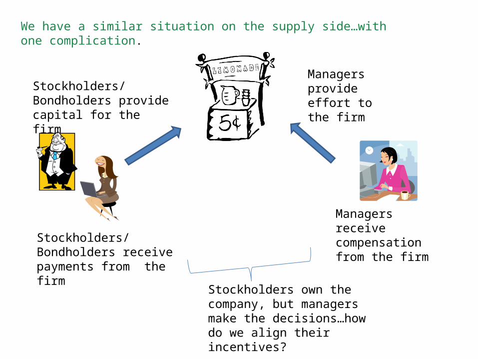
We have a similar situation on the supply side…with one complication.
Managers receive compensation from the firm
Managers provide effort to the firm
Stockholders/Bondholders provide capital for the firm
Stockholders/Bondholders receive payments from the firm
Stockholders own the company, but managers make the decisions…how do we align their incentives?
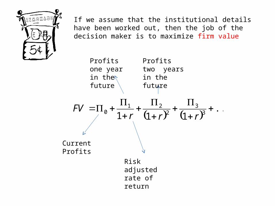
If we assume that the institutional details have been worked out, then the job of the decision maker is to maximize firm value
...
111 33
221
0
rrr
FV
Current Profits
Profits one year in the future
Risk adjusted rate of return
Profits two years in the future

While it is not necessary, it is sufficient to say that maximizing each year’s profits will maximize firm value
FCVCQPL
Price times quantity equals current revenues
Fixed costs (overhead) is not affected by the level of sales and, hence, has no impact on sales decisions
Variable costs are influenced by sales decisions
As with the average consumer, a firm’s decisions are made at the margin!!!

For each sale that is made, it must be profitable at the margin. For now, lets assume that the firm has no control over the price it charges
FCVCQPL
As with the average consumer, a firm’s decisions are made at the margin!!!
How does an additional sale affect revenues?
How does an additional sale affect costs?
LP MC
A sale will be made as long as it has a bigger impact on revenues than costs.

In either case, we can say that, given a representation of a firm’s cost structure, price should have a positive relationship with sales (higher price raises profit margin) while anything that influences costs at the margin should have a negative relationship with sales
Rational Behavior
MCPSQ LS ,(-)
Sales of lemonade are positively related to the price of lemonade and negatively related to marginal costs
FCVCQPL
Costs are a function of wages, material prices, etc.
(+)

A Demand Function represents the rational decisions made by a representative consumer(s)
IPDQ LD ,Quantity Purchased
“Is a function of”
Market Price (-)
Income (+)
For example, suppose that at a market price of $2.50, an individual with an annual income of $50,000 chooses to buy 5 glasses of lemonade per week.
000,50,$50.2$5 D

A Demand Curve is simply a graphical representation of a demand function
For example, suppose that at a market price of $2.50, an individual with an annual income of $50,000 chooses to buy 5 glasses of lemonade per week.
000,50,$50.2$5 D
Quantity
Price
$2.50
5
000,50$ID

A Demand Curve is simply a graphical representation of a demand function
Suppose that an increase in the market price from $2.50 to $2.75 causes this individual to reduce his/her lemonade purchases to 4 glasses per week
000,50,$75.2$4 D
Quantity
Price
$2.50
5
000,50$ID
$2.75
4
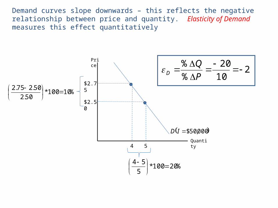
Demand curves slope downwards – this reflects the negative relationship between price and quantity. Elasticity of Demand measures this effect quantitatively
Quantity
Price
$2.50
5
000,50$ID
$2.75
4
%20100*5
54
%10100*50.2
50.275.2
210
20
%
%
P
QD

A Supply Function represents the rational decisions made by a representative firm(s)
MCPSQ LS ,Quantity Supplied
“Is a function of”
Market Price (+)
Marginal Costs (-)
For example, suppose that at a market price of $2.00, a firm facing a wage rate of $6/hr will supply 200 glasses per week.
6,$00.2$200 S

A Supply Curve is simply a graphical representation of a supply function
Quantity
Price
$2.00
200
6$CS
For example, suppose that at a market price of $3.00, a firm facing a wage rate of $6/hr will supply 200 glasses of lemonade per week.
6,$00.3$200 S
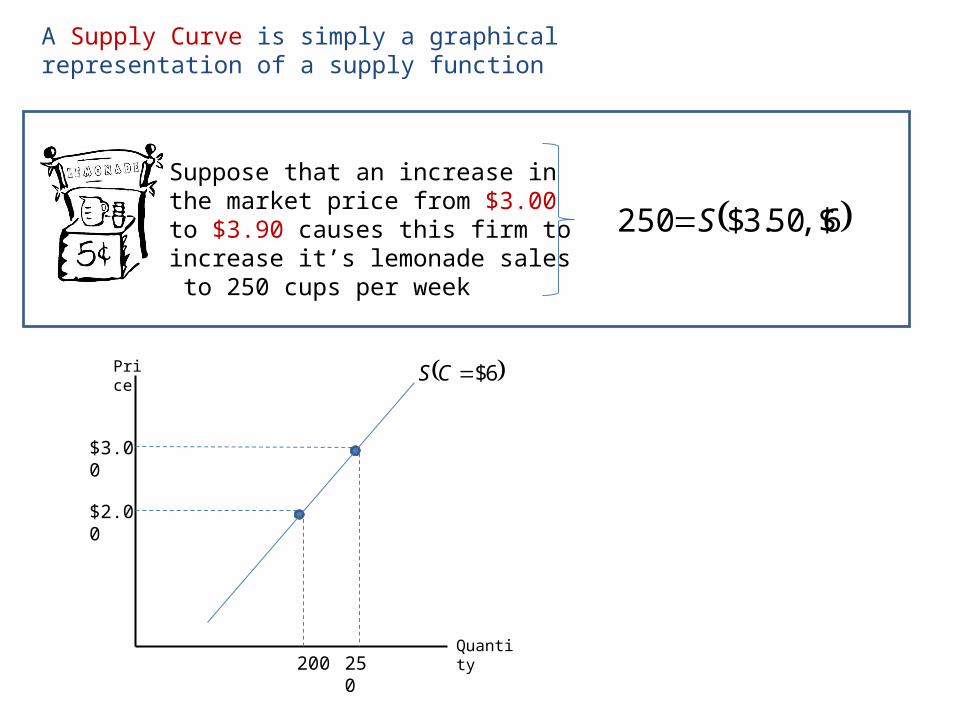
A Supply Curve is simply a graphical representation of a supply function
Suppose that an increase in the market price from $3.00 to $3.90 causes this firm to increase it’s lemonade sales to 250 cups per week
Quantity
Price
$2.00
200
6$CS
$3.00
250
6,$50.3$250 S
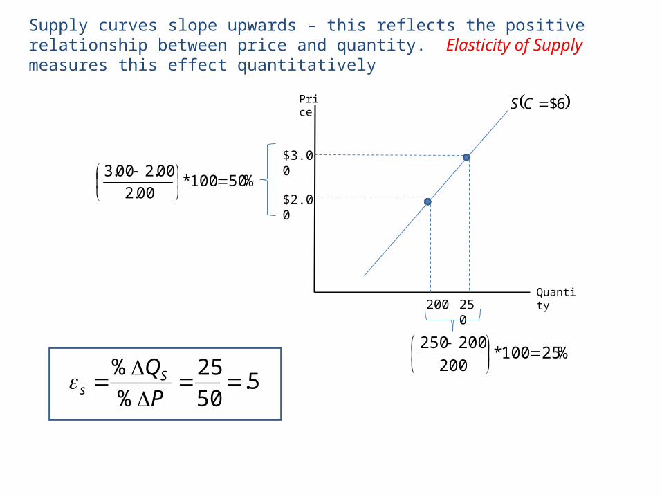
Supply curves slope upwards – this reflects the positive relationship between price and quantity. Elasticity of Supply measures this effect quantitatively
%25100*200
200250
%50100*00.2
00.200.3
5.50
25
%
%
P
QSs
Quantity
Price
$2.00
200
6$CS
$3.00
250

Quantity
Price
$2.00
6$CS
$3.00
Quantity
Price
25,000
000,50$ID
20,000 25,000
$2.50
$2.75
20,000
Suppose that the overall market consists of 5,000 identical lemonade drinkers and 100 lemonade suppliers
At a price of $2.50, each of the 5,000 lemonade drinkers buys 5 glasses per week.
At a price of $3.00, each of the 100 lemonade suppliers is willing to sell 250 glasses per week.
Quantity
Price
000,50$ID
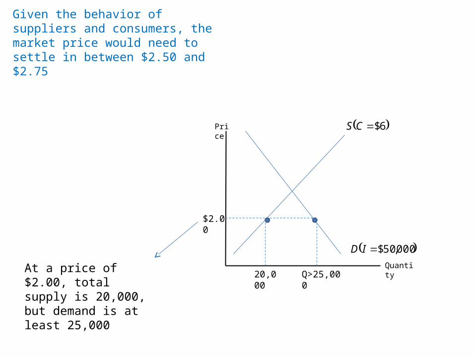
Given the behavior of suppliers and consumers, the market price would need to settle in between $2.50 and $2.75
6$CS
$2.00
20,000 Q>25,000At a price of $2.00, total supply is 20,000, but demand is at least 25,000

Quantity
Price
000,50$ID
Given the behavior of suppliers and consumers, the market price would need to settle in between $2.50 and $2.75
6$CS
$3.00
Q<20,000 25,000
At a price of $3.00, total supply is 25,000, but demand is less than 20,000

Quantity
Price
000,50$ID
Given the behavior of suppliers and consumers, the market price would need to settle in between $2.50 and $2.75
6$CS
$2.60
22,500
We would call the $2.60 price the equilibrium price
000,50$,60.2$6$,60.2$500,22 IDCS
Quantity
Price
000,50$ID
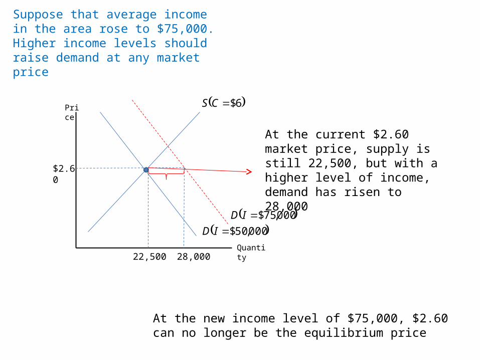
Suppose that average income in the area rose to $75,000. Higher income levels should raise demand at any market price
6$CS
$2.60
22,500
000,75$ID
28,000
At the current $2.60 market price, supply is still 22,500, but with a higher level of income, demand has risen to 28,000
At the new income level of $75,000, $2.60 can no longer be the equilibrium price

Quantity
Price
000,50$ID
Suppose that average income in the area rose to $75,000. Higher income levels should raise demand at any market price
6$CS
$2.60
22,500
000,75$ID
25,000
The increase in income causes a rise in sales and a rise in market price
$3.00 000,75$,00.3$6$,00.3$000,25 IDCS

Quantity
Price
000,50$ID
Suppose that lemonade store wages rose to $10/hr. Higher wages should lower supply at any market price
6$CS
$2.60
22,50018,000
At the current $2.60 market price, supply has fallen to 18,000, but demand is still at 22,500
At the wage level of $10, $2.60 can no longer be the equilibrium price

Quantity
Price
000,50$ID
Suppose that lemonade store wages rose to $10/hr. Higher wages should lower supply at any market price
6$CS
$2.60
22,50020,000
Higher wages cause a rise in market price and a drop in sales
$2.75 000,50$,75.2$10$,75.2$000,20 IDCS
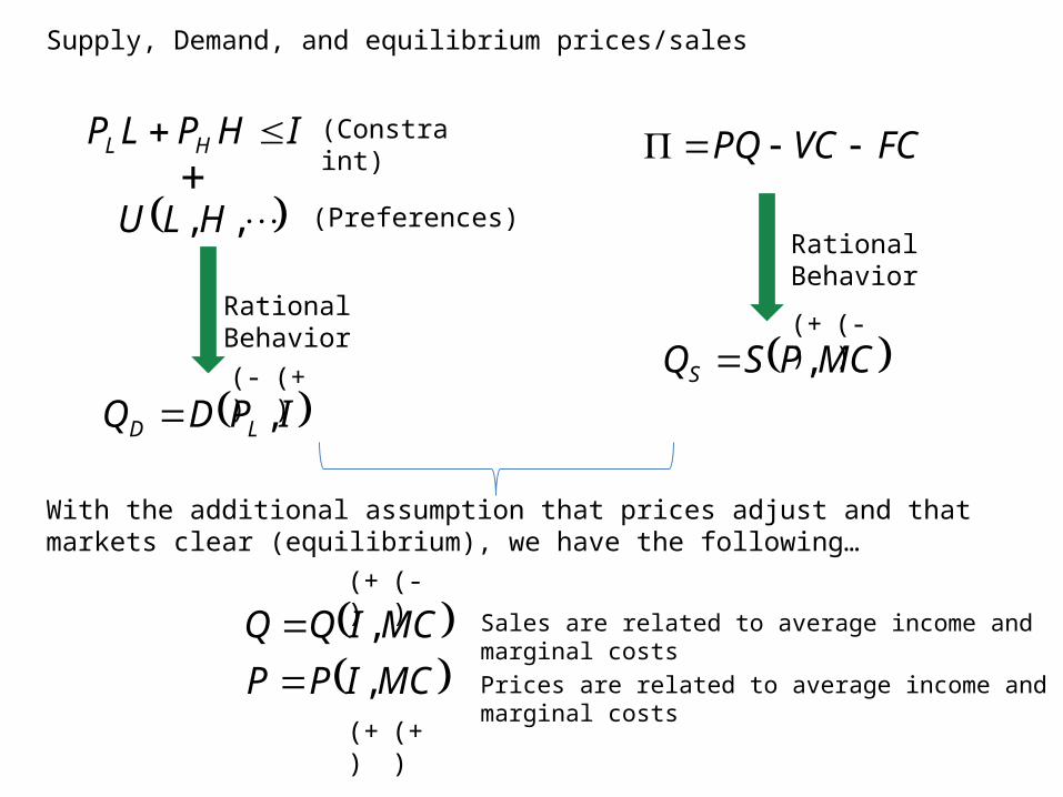
Supply, Demand, and equilibrium prices/sales
IHPLP HL
,,HLU (Preferences)
Rational Behavior
IPDQ LD ,(-) (+)
+(Constraint)
MCPSQS ,(-)
FCVCPQ
(+)
Rational Behavior
With the additional assumption that prices adjust and that markets clear (equilibrium), we have the following…
MCIPP
MCIQQ
,
,
(+) (-)
(+) (+)
Sales are related to average income and marginal costs
Prices are related to average income and marginal costs
Quantity
Price S
D
60.2$* P
500,22* Q
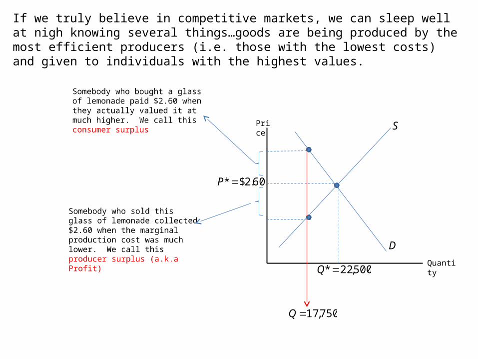
If we truly believe in competitive markets, we can sleep well at nigh knowing several things…goods are being produced by the most efficient producers (i.e. those with the lowest costs) and given to individuals with the highest values.
750,17Q
Somebody who bought a glass of lemonade paid $2.60 when they actually valued it at much higher. We call this consumer surplus
Somebody who sold this glass of lemonade collected $2.60 when the marginal production cost was much lower. We call this producer surplus (a.k.a Profit)

Quantity
Price S
D
60.2$* P
500,22* Q
We also can rest assured that we are producing exactly the right goods and services
Quantity
Price S
D
60.2$* P
500,22* Q
Hot DogsLemonade
If consumer preferences suddenly shifted away from lemonade and towards hot dogs, the lemonade market would shrink (as the price of lemonade falls) while the hot dog market expands (and the price rises)
'D
'D

High School Teacher: Salary = $50,000
Kobe Bryant: Salary = $23,000,000,000
Can we use our market model to explain differences in salaries?
Quantity
Price
D
S
$23M
1
Quantity
Price
D
S$50K
3,000,000$15K

Microsoft’s new Xbox 360 gaming console was released in North America on November 22 at a retail price of $299.99. Available supply sold out almost immediately as Christmas shoppers stood in line for this year’s hot item. (Microsoft has increased its sales target from 3M units to 6M units).
What’s odd about this??

Quantity
Price
D
3M
Clearly, $299.99 is not an equilibrium price !
S
???
$299.99
Why didn’t Microsoft raise their price?

When do our rationality assumptions begin to break down?
Situations involving interactions among small groups of people: Example: How to split $20.
Situations involving the immediate present vs. the future: Example: Instant gratification and the time value of money
Situations involving uncertaintyExample: The Monty Hall Problem

And now for something completely different….
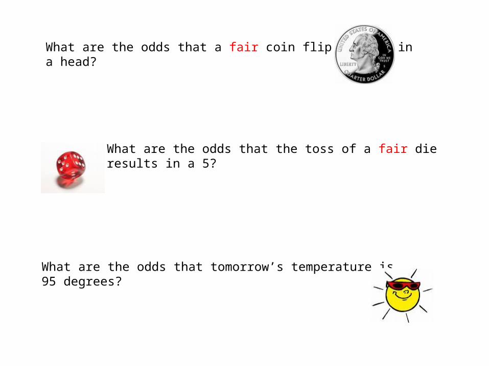
What are the odds that a fair coin flip results in a head?
What are the odds that the toss of a fair die results in a 5?
What are the odds that tomorrow’s temperature is 95 degrees?
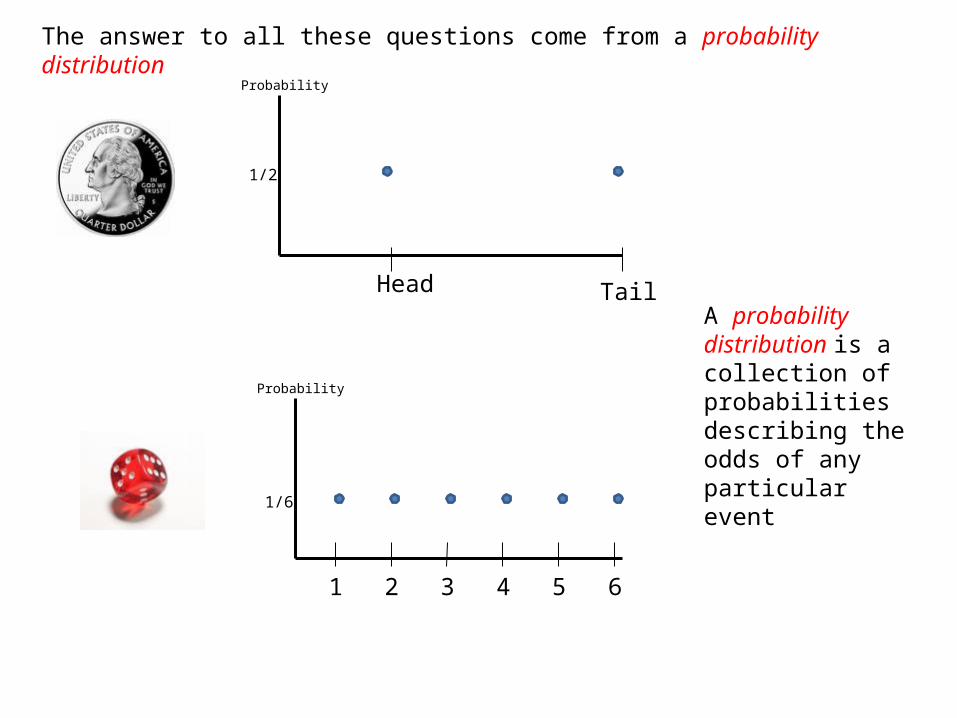
The answer to all these questions come from a probability distribution
Head Tail
1/2
Probability
1 6
1/6
Probability
2 3 4 5
A probability distribution is a collection of probabilities describing the odds of any particular event

The distribution for temperature in south bend is a bit more complicated because there are so many possible outcomes, but the concept is the same
Probability
Temperature
We generally assume a Normal Distribution which can be characterized by a mean (average) and standard deviation (measure of dispersion)
Mean
Standard Deviation

Probability
Temperature
Without some math, we can’t find the probability of a specific outcome, but we can easily divide up the distribution
Mean Mean+1SD Mean+2SDMean -1SDMean-2SD
2.5% 2.5%13.5% 34% 34% 13.5%

Annual Temperature in South Bend has a mean of 59 degrees and a standard deviation of 18 degrees.
Probability
Temperature59 77 954123
95 degrees is 2 standard deviations to the right – there is a 2.5% chance the temperature is 95 or greater (97.5% chance it is cooler than 95)
Can’t we do a little better than this?

Conditional distributions give us probabilities conditional on some observable information – the temperature in South Bend conditional on the month of July has a mean of 84 with a standard deviation of 7.
Probability
Temperature84 91 987770
95 degrees falls a little more than one standard deviation away (there approximately a 16% chance that the temperature is 95 or greater)
95
Conditioning on month gives us a more accurate forecast!

5.PrPr TailsHeads
We know that there should be a “true” probability distribution that governs the outcome of a coin toss (assuming a fair coin)
Suppose that we were to flip a coin over and over again and after each flip, we calculate the percentage of heads & tails
FlipsTotal
Headsof
#5.
That is, if we collect “enough” data, we can eventually learn the truth!
(Sample Statistic) (True Probability)

We can follow the same process for the temperature in South Bend
Temperature ~ 2,N
We could find this distribution by collecting temperature data for south bend
N
iixN
x1
1
2
1
22 1
N
ii xx
Ns
Sample Mean
(Average)
Sample Variance
Note: Standard Deviation is the square root of the variance.
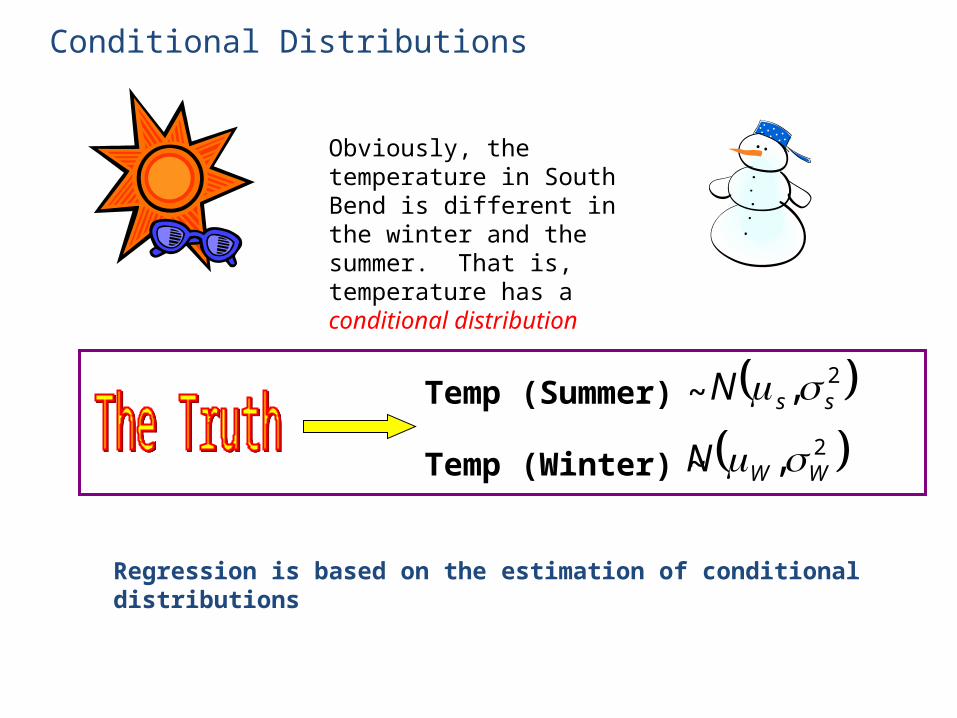
Conditional Distributions
Obviously, the temperature in South Bend is different in the winter and the summer. That is, temperature has a conditional distribution
Temp (Summer) ~ 2, ssN
Temp (Winter) ~ 2, WWN
Regression is based on the estimation of conditional distributions

Mean = 1
Variance = 4
Std. Dev. = 2
Probability distributions are scalable
22
2
σ,kkNy
kxy
μ,σNx
3 X =
Mean = 3
Variance = 36 (3*3*4)
Std. Dev. = 6
Some useful properties of probability distributions
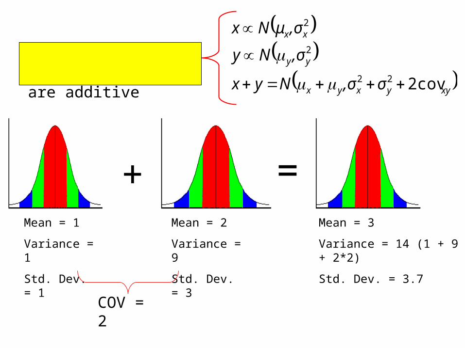
Mean = 1
Variance = 1
Std. Dev. = 1
Probability distributions are additive
xyyxyx
yy
xx
σ,σNyx
,σNy
,σμNx
cov222
2
2
+Mean = 2
Variance = 9
Std. Dev. = 3
COV = 2
=Mean = 3
Variance = 14 (1 + 9 + 2*2)
Std. Dev. = 3.7

Mean = 8
Variance = 4
Std. Dev. = 2
Mean = $ 12,000
Variance = 4,000,000
Std. Dev. = $ 2,000
Suppose we know that the value of a car is determined by its age
Value = $20,000 - $1,000 (Age)
Car Age Value

We could also use this to forecast:
Value = $20,000 - $1,000 (Age)
How much should a six year old car be worth?
Value = $20,000 - $1,000 (6) = $14,000
Note: There is NO uncertainty in this prediction.

Searching for the truth….
You believe that there is a relationship between age and value, but you don’t know what it is….
1. Collect data on values and age
2. Estimate the relationship between them
Note that while the true distribution of age is N(8,4), our collected sample will not be N(8,4). This sampling error will create errors in our estimates!!

Value = a + b * (Age) + error 20,σNerror
We want to choose ‘a’ and ‘b’ to minimize the error!
a
Slope = b
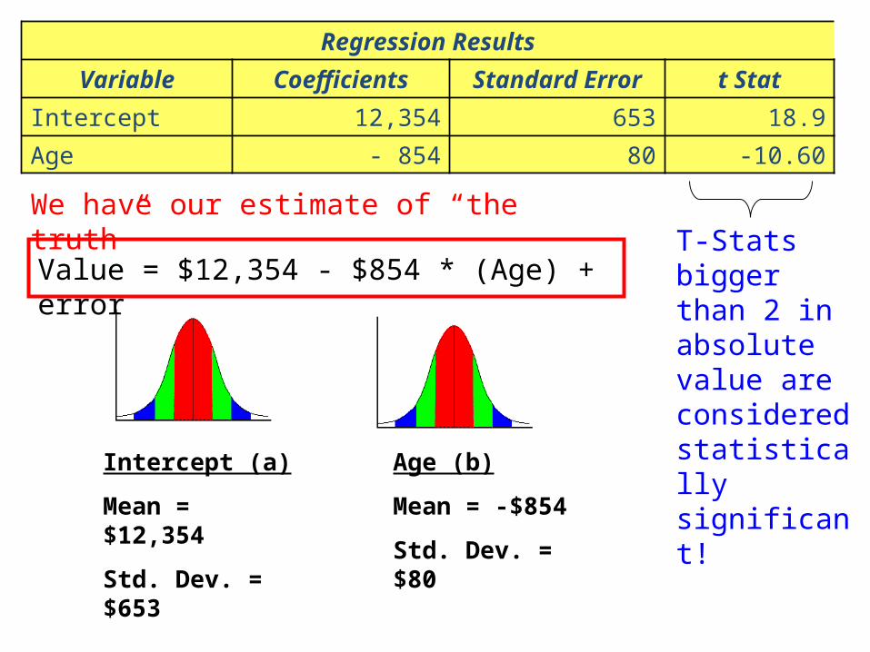
Regression Results
Variable Coefficients Standard Error t Stat
Intercept 12,354 653 18.9
Age - 854 80 -10.60
Value = $12,354 - $854 * (Age) + error
We have our estimate of “the truth”
Intercept (a)
Mean = $12,354
Std. Dev. = $653
Age (b)
Mean = -$854
Std. Dev. = $80
T-Stats bigger than 2 in absolute value are considered statistically significant!
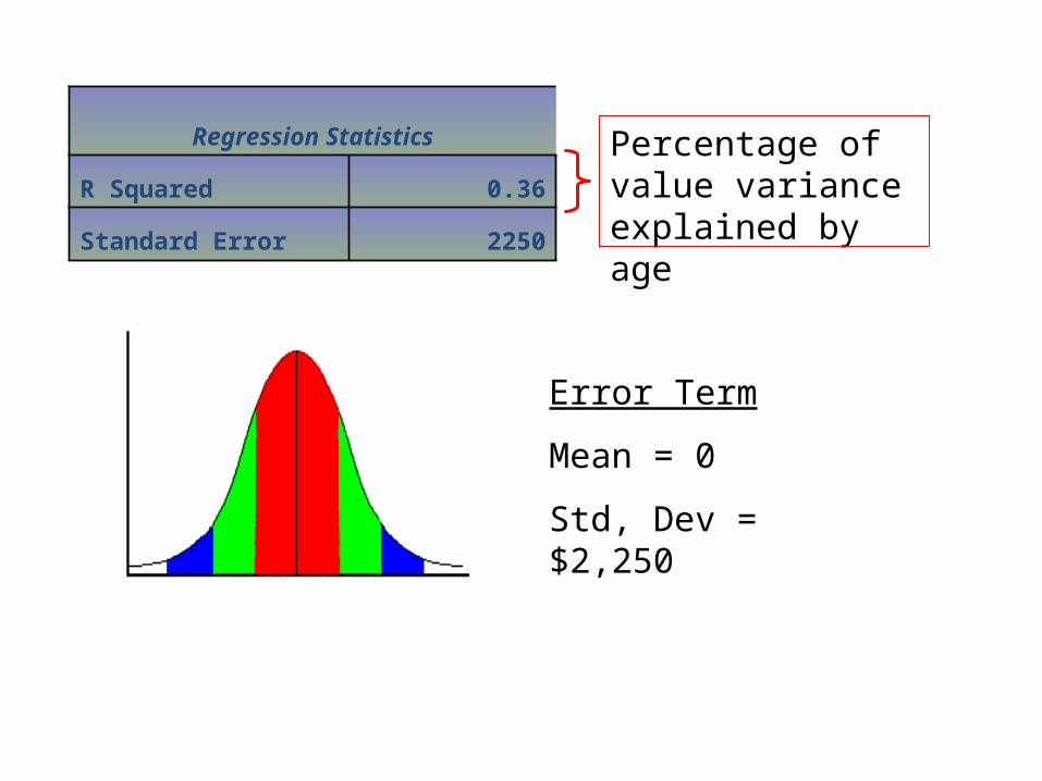
Regression Statistics
R Squared 0.36
Standard Error 2250
Error Term
Mean = 0
Std, Dev = $2,250
Percentage of value variance explained by age
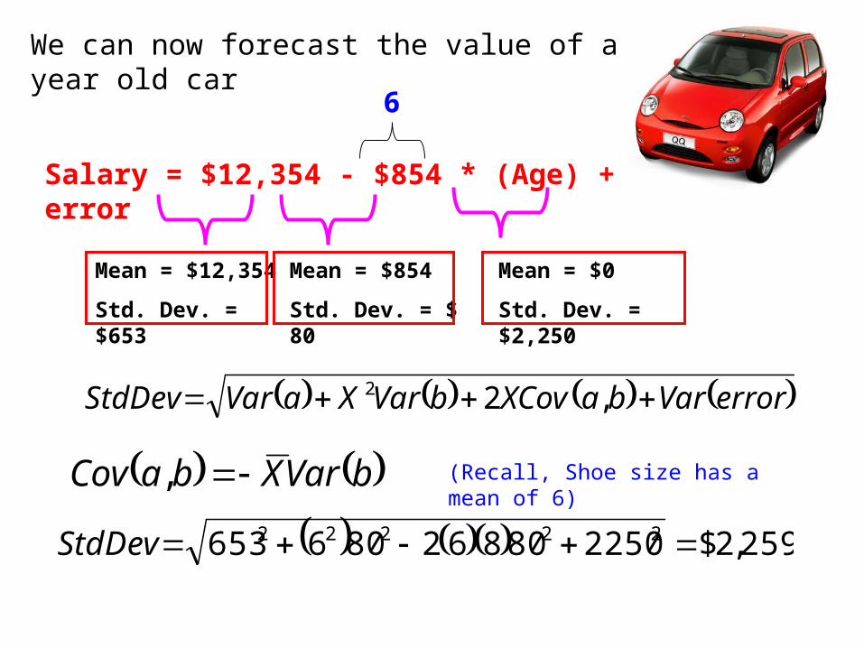
We can now forecast the value of a 6 year old car
Salary = $12,354 - $854 * (Age) + error
6
Mean = $12,354
Std. Dev. = $653
Mean = $854
Std. Dev. = $ 80
Mean = $0
Std. Dev. = $2,250
errorVarbaXCovbVarXaVarStdDev ,22
bVarXbaCov , (Recall, Shoe size has a mean of 6)
259,2$225080862806653 22222 StdDev

8x
+95%
-95%
Age
Value
Note that your forecast error will always be smallest at the sample mean! Also, your forecast gets worse at an increasing rate as you depart from the mean
6Age
Forecast Interval
259,2$225080862806653 22222 StdDev
230,7$6*854354,12 Value
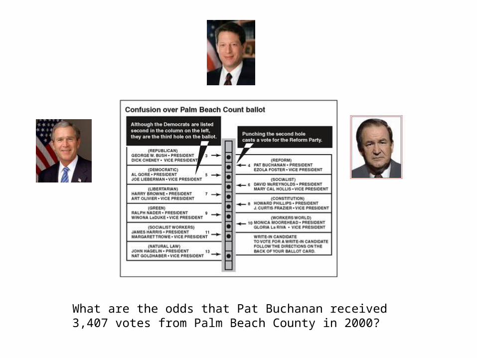
What are the odds that Pat Buchanan received 3,407 votes from Palm Beach County in 2000?

The Strategy: Estimate a conditional distribution for Pat Buchanan’s votes using every county EXCEPT Palm Beach
Using Palm Beach data, forecast Pat Buchanan’s vote total for Palm Beach
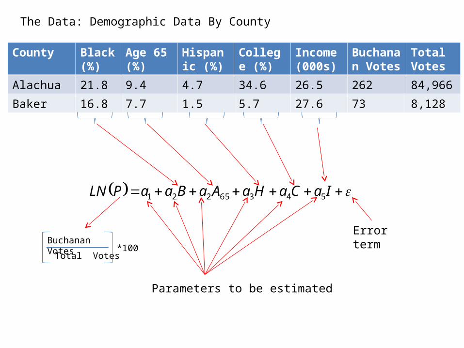
The Data: Demographic Data By County
County Black (%)
Age 65 (%)
Hispanic (%)
College (%)
Income (000s)
Buchanan Votes
Total Votes
Alachua 21.8 9.4 4.7 34.6 26.5 262 84,966
Baker 16.8 7.7 1.5 5.7 27.6 73 8,128
IaCaHaAaBaaPLN 54365221
Parameters to be estimated
Error termBuchanan Votes
Total Votes*100

Side note: Why logs?
BP 5.3
P = Buchanan’s Vote PercentageB = Percentage Black
Option #1: Linear
BPLN 5.3
Option #2: Semi –Log Linear
BLNPLN 5.3
Option #3: Log Linear
A 10% increase in the black percentage (say, from 30% to 40%) increases Pat Buchanan’s vote percentage by 5% (Say, from 1% to 6%)
A 10% increase in the black percentage (say, from 30% to 40%) increases Pat Buchanan’s vote percentage by 5% (Say, from 1% to 1(1.05) = 1.05%)
A 10% increase in the black percentage (say, from 30% 30(1.10) = 33% increases Pat Buchanan’s vote percentage by 5% (Say, from 1(1.05) = 1.05%)

The Results:
Variable Coefficient Standard Error t - statistic
Intercept 2.146 .396 5.48
Black (%) -.0132 .0057 -2.88
Age 65 (%) -.0415 .0057 -5.93
Hispanic (%) -.0349 .0050 -6.08
College (%) -.0193 .0068 -1.99
Income (000s) -.0658 .00113 -4.58
Now, we can make a forecast!
ICHABPLN 0658.0193.0349.0415.0132.146.2 65

County Black (%)
Age 65 (%)
Hispanic (%)
College (%)
Income (000s)
Buchanan Votes
Total Votes
Palm Beach 21.8 23.6 9.8 22.1 33.5 3,407 431,621
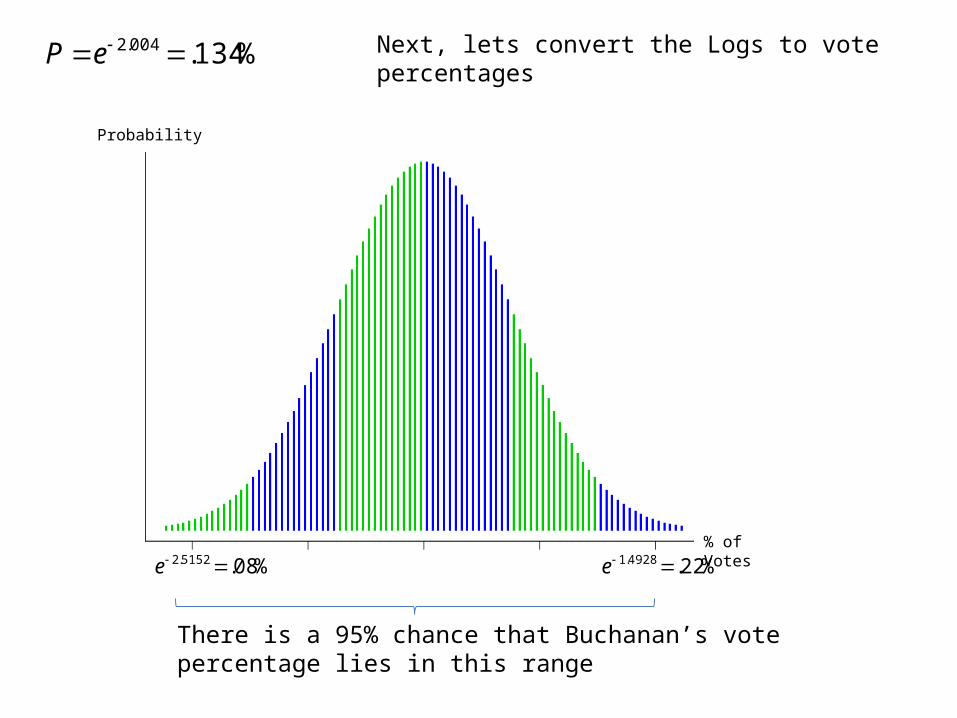
004.2PLN
%134.004.2 eP
578621,43100134. This would be our prediction for Pat Buchanan’s vote total!
ICHABPLN 0658.0193.0349.0415.0132.146.2 65

Probability
LN(%Votes)
There is a 95% chance that the log of Buchanan’s vote percentage lies in this range
-2.004 – 2*(.2556) -2.004 + 2*(.2556)= -2.5152 = -1.4928
004.2PLN We know that the log of Buchanan’s vote percentage is distributed normally with a mean of -2.004 and with a standard deviation of .2556
Probability
% of Votes
There is a 95% chance that Buchanan’s vote percentage lies in this range
%134.004.2 eP
%08.5152.2 e %22.4928.1 e
Next, lets convert the Logs to vote percentages

Probability
Votes
There is a 95% chance that Buchanan’s total vote lies in this range
348621,4310008. 970621,4310022.
Finally, we can convert to actual votes 578621,43100134.


