ECP Milestone Report Initial Integration of CEED Software ... · ECP Milestone Report Initial...

ECP Milestone Report

Initial Integration of CEED Software in ECP Applications

WBS 1.2.5.3.04, Milestone CEED-MS8

Misun MinJed Brown

Veselin DobrevPaul FischerTzanio KolevDavid MedinaElia MerzariAleks ObabkoScott ParkerRon Rahaman

Stanimire TomovVladimir TomovTim Warburton

October 4, 2017

DOCUMENT AVAILABILITY

Reports produced after January 1, 1996, are generally available free via US Department ofEnergy (DOE) SciTech Connect.

Website http://www.osti.gov/scitech/

Reports produced before January 1, 1996, may be purchased by members of the publicfrom the following source:

National Technical Information Service5285 Port Royal RoadSpringfield, VA 22161Telephone 703-605-6000 (1-800-553-6847)TDD 703-487-4639Fax 703-605-6900E-mail [email protected] http://www.ntis.gov/help/ordermethods.aspx

Reports are available to DOE employees, DOE contractors, Energy Technology DataExchange representatives, and International Nuclear Information System representativesfrom the following source:

Office of Scientific and Technical InformationPO Box 62Oak Ridge, TN 37831Telephone 865-576-8401Fax 865-576-5728E-mail [email protected] http://www.osti.gov/contact.html

This report was prepared as an account of work sponsored by an agencyof the United States Government. Neither the United States Governmentnor any agency thereof, nor any of their employees, makes any warranty,express or implied, or assumes any legal liability or responsibility forthe accuracy, completeness, or usefulness of any information, apparatus,product, or process disclosed, or represents that its use would not infringeprivately owned rights. Reference herein to any specific commercialproduct, process, or service by trade name, trademark, manufacturer,or otherwise, does not necessarily constitute or imply its endorsement,recommendation, or favoring by the United States Government or anyagency thereof. The views and opinions of authors expressed herein donot necessarily state or reflect those of the United States Government orany agency thereof.




Office of Advanced Scientific Computing ResearchOffice of Science

US Department of Energy

Office of Advanced Simulation and ComputingNational Nuclear Security Administration

US Department of Energy

October 4, 2017

Exascale Computing Project (ECP) iii CEED-MS8




Approvals

Submitted by:

Tzanio Kolev, LLNL DateCEED PI

Approval:

Douglas B. Kothe, Oak Ridge National Laboratory DateDirector, Applications DevelopmentExascale Computing Project

Exascale Computing Project (ECP) iv CEED-MS8

Revision Log

Version Creation Date Description Approval Date

1.0 October 4, 2017 Original

Exascale Computing Project (ECP) v CEED-MS8

EXECUTIVE SUMMARY

Key components of CEED software development involve fast finite element operator storage and evaluation,architecture optimizations, performant algorithms for all orders, global kernels for finite element operators,efficient use of the memory sub-system, optimal data locality and motion, enhanced scalability and parallelism,and fast tensor contractions. As ultimate goals of the project, CEED is exploring and identifying the bestalgorithms for the full range of discretizations and applying algorithmic and software development to supportECP applications’ needs.

In this milestone we report on the initial integration of CEED software in the selected first-wave ECP/CEEDapps and the continued exploration of other ECP applications as second-wave (milestone CEED-MS23) andthird-wave (milestone CEED-MS35) ECP/CEED application candidates. An extensive evaluation of variousapproaches for GPU acceleration of the CEED computational motives is also a major focus of the report, bothin the settings of CEED’s Nekbone and Laghos miniapps, as well as versions of CEED’s bake-off problems(introduced in milestone CEED-MS6).

The first-wave ECP applications targeted for coupling with CEED software include the ExaSMR andMARBL applications. We also report on near-term collaboration with the seed-funded Urban Systems project,as well as engagements with ACME, ExaAM, GEOS and the Application Assessment and Proxy App projects.

The ExaSMR project involves coupled thermal-hydraulics/neutronics, with the latter based on MonteCarlo methods and the former based on high-order discretizations of the Navier-Stokes and energy equationsfor accurate simulation of turbulent transport. The project requires fast and efficient turbulence simulationcapabilities that will scale to exascale platforms. Work within CEED will ensure that all aspects of theNek5000 workflow scale to the target problem space, which involves > 1010 degrees of freedom in typicalproduction runs. CEED’s goal is to provide implementations that perform with maximum attainable efficiencyand deliver low turn-around times. A deliverable for this milestone is beta-release of the GPU-based variantof Nek5000.

MARBL is targeting high-energy-density physics problems, including single fluid multi-material hydro-dynamics and radiation/magnetic diffusion simulation, with applications in inertial confined fusion, pulsedpower experiments, and equation of state/material strength analysis. The code uses high-order methods basedarbitrary Lagrangian-Eulerian, direct Eulerian, and unstructured adaptive mesh refinement. A deliverablefor this milestone is collaboration with MARBL for improved performance based on partially-assembledoperators.

The Urban exascale project is planning to couple real-time data with high performance simulations tostudy particulate transport in cities. Nek5000 will be used for large eddy and RANS (Reynolds-averagedNavier-Stokes) simulations of turbulent transport in these domains. Areas where the CEED team is aidingthe Urban Canyon group include creating high-order meshes for urban geometries and developing boundaryconditions appropriate for simulations close to real-life urban conditions.

The software artifacts delivered as part of this milestone include GPU-enabled versions of the Nekboneand Laghos miniapps, which are provided through the CEED website, http://ceed.exascaleproject.organd the CEED GitHub organization, http://github.com/ceed.

In addition to details and results from the above R&D efforts, in this document we are also reportingon other project-wide activities performed in Q4 of FY17, including: the CEED first annual meeting andparticipation of CEED researchers in a variety of outreach activities.

Exascale Computing Project (ECP) vi CEED-MS8

http://ceed.exascaleproject.org

http://github.com/ceed

TABLE OF CONTENTS

Executive Summary vi

List of Figures viii

List of Tables x

1 Introduction 1

2 ECP Applications 12.1 MARBL . . . . . . . . . . . . . . . . . . . . . . . . . . . . . . . . . . . . . . . . . . . . . . . . 1

2.1.1 Plan and Timeline for CEED Activities . . . . . . . . . . . . . . . . . . . . . . . . . . 12.1.2 Refactoring of MARBL/BLAST’s Lagrange phase . . . . . . . . . . . . . . . . . . . . 2

2.2 ExaSMR . . . . . . . . . . . . . . . . . . . . . . . . . . . . . . . . . . . . . . . . . . . . . . . . 32.2.1 Nek5000 GPU Implementation . . . . . . . . . . . . . . . . . . . . . . . . . . . . . . . 32.2.2 Nek5000 GPU/CPU Verification and Performance on ExaSMR Tests . . . . . . . . . . 4

2.3 Other ECP Applications . . . . . . . . . . . . . . . . . . . . . . . . . . . . . . . . . . . . . . . 62.3.1 Urban . . . . . . . . . . . . . . . . . . . . . . . . . . . . . . . . . . . . . . . . . . . . . 62.3.2 ACME . . . . . . . . . . . . . . . . . . . . . . . . . . . . . . . . . . . . . . . . . . . . . 72.3.3 ExaAM . . . . . . . . . . . . . . . . . . . . . . . . . . . . . . . . . . . . . . . . . . . . 82.3.4 GEOS . . . . . . . . . . . . . . . . . . . . . . . . . . . . . . . . . . . . . . . . . . . . . 82.3.5 Combustion . . . . . . . . . . . . . . . . . . . . . . . . . . . . . . . . . . . . . . . . . . 8

2.4 ECP Application Assessment . . . . . . . . . . . . . . . . . . . . . . . . . . . . . . . . . . . . 92.4.1 Nek5000 Full Application Weak and Strong Scaling . . . . . . . . . . . . . . . . . . . . 92.4.2 NekBench Utilities for Scaling Studies . . . . . . . . . . . . . . . . . . . . . . . . . . . 9

3 Miniapps 93.1 Laghos . . . . . . . . . . . . . . . . . . . . . . . . . . . . . . . . . . . . . . . . . . . . . . . . . 9

3.1.1 A GPU Version of MFEM Based on OCCA . . . . . . . . . . . . . . . . . . . . . . . . 103.1.2 Laghos on OCCA . . . . . . . . . . . . . . . . . . . . . . . . . . . . . . . . . . . . . . . 11

3.2 Nekbone . . . . . . . . . . . . . . . . . . . . . . . . . . . . . . . . . . . . . . . . . . . . . . . . 123.2.1 Introduction and Algorithm . . . . . . . . . . . . . . . . . . . . . . . . . . . . . . . . . 12

3.3 CORAL-2 Benchmarks and Vendor Interactions . . . . . . . . . . . . . . . . . . . . . . . . . . 16

4 GPU Performance Optimization 174.1 OCCA . . . . . . . . . . . . . . . . . . . . . . . . . . . . . . . . . . . . . . . . . . . . . . . . . 174.2 Background in GPU Acceleration of Finite Element Computations . . . . . . . . . . . . . . . 184.3 Notation . . . . . . . . . . . . . . . . . . . . . . . . . . . . . . . . . . . . . . . . . . . . . . . . 194.4 BP1.0: Mass Matrix Multiplication . . . . . . . . . . . . . . . . . . . . . . . . . . . . . . . . . 20

4.4.1 BP1.0 Mathematical Formulation . . . . . . . . . . . . . . . . . . . . . . . . . . . . . . 204.4.2 BP1.0 Implementation . . . . . . . . . . . . . . . . . . . . . . . . . . . . . . . . . . . . 22

4.5 BP3.5: Stiffness Matrix with Collocation Differentiation . . . . . . . . . . . . . . . . . . . . . 254.5.1 BP3.5 mathematical formulation . . . . . . . . . . . . . . . . . . . . . . . . . . . . . . 254.5.2 BP3.5 Implementation . . . . . . . . . . . . . . . . . . . . . . . . . . . . . . . . . . . . 26

4.6 BP3.0: Stiffness Matrix A Evaluated with Quadrature . . . . . . . . . . . . . . . . . . . . . . 314.6.1 BP3.0 Mathematical Formulation . . . . . . . . . . . . . . . . . . . . . . . . . . . . . . 31

4.7 Summary and Future Work . . . . . . . . . . . . . . . . . . . . . . . . . . . . . . . . . . . . . 34

5 Other Project Activities 355.1 CEED First Annual Meeting . . . . . . . . . . . . . . . . . . . . . . . . . . . . . . . . . . . . 355.2 Outreach . . . . . . . . . . . . . . . . . . . . . . . . . . . . . . . . . . . . . . . . . . . . . . . 36

6 Conclusion 36

Exascale Computing Project (ECP) vii CEED-MS8

LIST OF FIGURES

1 Integration plan and milestones for CEED/BLAST activities. . . . . . . . . . . . . . . . . . . 22 ExaSMR spectral element hexahedral meshes for subchannel and full assembly systems with

2× 2 (left) and 17× 17 (right) rods. . . . . . . . . . . . . . . . . . . . . . . . . . . . . . . . . 33 Nek5000 fully GPU-ported runs with validation for different boundary conditions for 3D eddy

simulations, demonstrating spectral convergence as increasing N = 3, 5, 7, 9, 11, 13, 15 withE = 4× 4× 3 at time step 50; A single-rod mesh with N = 7 and E = 2560 demonstratingpressure solve iteration counts for 1000 step runs with validated results agreeing up to 12–14digits between CPU vs. GPU. . . . . . . . . . . . . . . . . . . . . . . . . . . . . . . . . . . . . 4

4 Nek5000 performance on SummitDev, Titan, and Theta. . . . . . . . . . . . . . . . . . . . . . 55 Preliminary LES results for a reference dataset of the flow over a small but representative

landscape that includes the Lake Point Tower building geometry. . . . . . . . . . . . . . . . . 76 Nek5000 weak-scale study: (left) example of a scalable multi-rod mesh, (right) weak-scale

performance on CETUS for varying problem sizes and coarse-grid solver choices. . . . . . . . 107 Laghos: 2D inversion of the global mass operator. . . . . . . . . . . . . . . . . . . . . . . . . 128 Laghos: 3D inversion of the global mass operator. . . . . . . . . . . . . . . . . . . . . . . . . 139 Laghos: 2D application of the force operator. . . . . . . . . . . . . . . . . . . . . . . . . . . . 1310 Laghos: 3D application of the force operator. . . . . . . . . . . . . . . . . . . . . . . . . . . . 1311 Laghos: 2D update of quadrature data. . . . . . . . . . . . . . . . . . . . . . . . . . . . . . . 1312 Laghos: 3D update of quadrature data. . . . . . . . . . . . . . . . . . . . . . . . . . . . . . . 1413 Laghos: 2D total execution rates. . . . . . . . . . . . . . . . . . . . . . . . . . . . . . . . . . 1414 Laghos: 3D total execution rates. . . . . . . . . . . . . . . . . . . . . . . . . . . . . . . . . . 1415 Nekbone OpenMP results on a single node of Theta (KNL). . . . . . . . . . . . . . . . . . . . 1816 BP1.0: performance roofline bounds. The upper plot (line with diamond-shaped ticks) shows

theoretical bound obtained by using a theoretical peak bandwidth of 549GB/s for the NVIDIAP100 PCI-E 12GB GPU. The lower plot (line with circle-shaped ticks) shows the empiricalpeak bandwidth bound obtained by using the measured bandwidth attained when performinga device memory to device memory copy. Left: performance bounds for cubical mesh with512 hexahedral elements. Right: performance bounds for cubical mesh with 4, 096 hexahedralelements. . . . . . . . . . . . . . . . . . . . . . . . . . . . . . . . . . . . . . . . . . . . . . . . 22

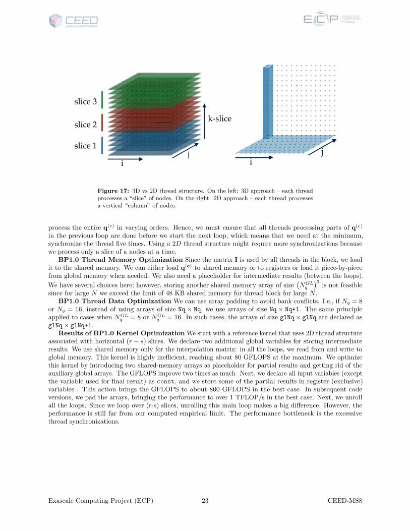
17 3D vs 2D thread structure. On the left: 3D approach – each thread processes a “slice” ofnodes. On the right: 2D approach – each thread processes a vertical “column” of nodes. . . 23

18 BP1.0: performance results for the code for BP1.0. Left: results obtained using cube-shapedmesh with 512 elements. Right: results obtained using cube-shaped mesh with 4,096 elementson a NVIDIA P100 PCI-E 12GB GPU. . . . . . . . . . . . . . . . . . . . . . . . . . . . . . . 24

19 BP1.0: the idea behind reducing synchronizations in kernel 9. We fetch pieces of qe to registersfrom shared memory and then write the result to shared memory. This action does not createrace conditions because we do use a 2D thread structure and interpolate only in one directionat a time. . . . . . . . . . . . . . . . . . . . . . . . . . . . . . . . . . . . . . . . . . . . . . . . 25

20 BP3.5: performance roofline bounds. The upper plot (line with diamond-shaped ticks) showstheoretical bound obtained using theoretical peak bandwidth of 549GB/s on a single NVIDIAP100 PCI-E 12GB GPU. The lower plot (line with circle-shaped ticks) shows the boundobtained using bandwidth for device to device copy. Left: performance bounds for cubicalmesh with 512 elements. Right: performance bounds for cubical mesh with 4, 096 elements. . 28

21 BP3.5: Performance of 2D kernels in various stages of optimization. The red line marked withcrosses is the empirically determined roofline based on optimal achievable device to devicememory copies on an NVIDIA P100 PCI-E 12GB GPU. Left: GFLOPS for cubical mesh with512 elements. Right: GFLOPS for cubical mesh with 4, 096 elements. . . . . . . . . . . . . . 30

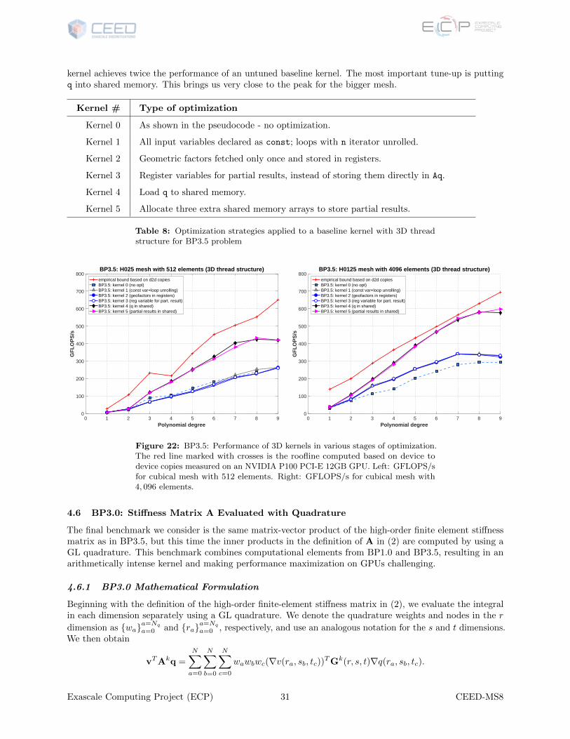
22 BP3.5: Performance of 3D kernels in various stages of optimization. The red line marked withcrosses is the roofline computed based on device to device copies measured on an NVIDIA P100PCI-E 12GB GPU. Left: GFLOPS/s for cubical mesh with 512 elements. Right: GFLOPS/sfor cubical mesh with 4, 096 elements. . . . . . . . . . . . . . . . . . . . . . . . . . . . . . . . 31

Exascale Computing Project (ECP) viii CEED-MS8

23 BP3.0: performance roofline bounds. The upper plot (line with diamond-shaped ticks) showstheoretical bound obtained using theoretical peack bandwidth of 549GB/s on an NVIDIA P100PCI-E 12GB GPU. The lower plot (line with circle-shaped ticks) shows the bound obtainedusing bandwidth for device to device copy. Left: performance bounds for cubical mesh with512 elements. Right: performance bounds for cubical mesh with 4, 096 elements. . . . . . . . 33

24 BP3.0: Performance of 2D kernels in various stages of optimization. The red line marked withcrosses is the roofline computed based on device to device copies on a single NVIDIA P100PCI-E 12GB GPU. Left: GFLOPS/s for cubical mesh with 512 elements. Right: GFLOPS/sfor cubical mesh with 4, 096 elements. . . . . . . . . . . . . . . . . . . . . . . . . . . . . . . . 34

25 BP3.0: Performance of 3D kernels in various stages of optimization. The red line marked withcrosses is the roofline computed based on device to device copies on a single NVIDIA P100PCI-E 12GB GPU. Left: GFLOPS/s for cubical mesh with 512 elements. Right: GFLOPS/sfor cubical mesh with 4096 elements. . . . . . . . . . . . . . . . . . . . . . . . . . . . . . . . . 35

Exascale Computing Project (ECP) ix CEED-MS8

LIST OF TABLES

1 Nek5000 single-rod run timings on P100 vs. Intel Xeon GHz (JLSE neddy/maud). . . . . . . 52 Compute systems overview for ExaSMR/Nek5000 runs . . . . . . . . . . . . . . . . . . . . . . 63 Performance model of CPU Nekbone . . . . . . . . . . . . . . . . . . . . . . . . . . . . . . . . 154 Comparison of KNL and P100 Statistics . . . . . . . . . . . . . . . . . . . . . . . . . . . . . . 165 Performance Analysis of Nekbone on KNL . . . . . . . . . . . . . . . . . . . . . . . . . . . . . 176 Performance Analysis of Nekbone on GPU . . . . . . . . . . . . . . . . . . . . . . . . . . . . . 177 Optimization strategies applied to a baseline kernel with 2D thread structure for BP3.5 problem 308 Optimization strategies applied to a baseline kernel with 3D thread structure for BP3.5 problem 319 Optimization strategies applied to a baseline kernel with 2D thread structure for BP3.0 problem 3410 Optimization strategies applied to a baseline kernel with 3D thread structure for BP3.0 problem 35

LIST OF ALGORITHMS

1 Improved Quadrature Evaluation for MARBL/BLAST . . . . . . . . . . . . . . . . . . . . . . 22 Conjugate Gradient Solver in Nekbone . . . . . . . . . . . . . . . . . . . . . . . . . . . . . . . 153 BP1.0: mass matrix multiplication . . . . . . . . . . . . . . . . . . . . . . . . . . . . . . . . . 214 BP3.5: collocation differentiation for 3D hexahedral mesh . . . . . . . . . . . . . . . . . . . . 275 BP3.5: starting point of the implementation (2D thread structure) . . . . . . . . . . . . . . . 296 BP3.5: collocation differentiation for 3D hexahedral mesh (3D thread structure) . . . . . . . 397 BP3.0: differentiation for 3D hexahedral elements . . . . . . . . . . . . . . . . . . . . . . . . . 40

Exascale Computing Project (ECP) x CEED-MS8

1. INTRODUCTION

Key components of CEED software development involve fast finite element operator storage and evaluation,architecture optimizations, performant algorithms for all orders, global kernels for finite element operators,efficient use of the memory sub-system, optimal data locality and motion, enhanced scalability and parallelism,and fast tensor contractions. As ultimate goals of the project, CEED is exploring and identifying the bestalgorithms for the full range of discretizations and applying algorithmic and software development to supportECP applications’ needs.

In this milestone we report on the initial integration of CEED software in the selected first-wave ECP/CEEDapps and the continued exploration of other ECP applications as second-wave (milestone CEED-MS23) andthird-wave (milestone CEED-MS35) ECP/CEED application candidates. An extensive evaluation of variousapproaches for GPU acceleration of the CEED computational motives is also a major focus of the report, bothin the settings of CEED’s Nekbone and Laghos miniapps, as well as versions of CEED’s bake-off problems(introduced in milestone CEED-MS6).

The software artifacts delivered as part of this milestone include GPU-enabled versions of the Nekboneand Laghos miniapps, which are provided through the CEED website, http://ceed.exascaleproject.organd the CEED GitHub organization, http://github.com/ceed.

2. ECP APPLICATIONS

The first-wave ECP applications targeted for coupling with CEED software include the ExaSMR and MARBLapplications. We also report on near-term collaboration with the seed-funded Urban Systems project, as wellas engagements with ACME, ExaAM, GEOS and the Application Assessment and Proxy App projects.

2.1 MARBL

As discussed in previous reports, the MARBL application has two major components, namely BLAST andMIRANDA. The CEED efforts are concentrated exclusively on BLAST, which is an MFEM-based ArbitraryLagrangian-Eulerian (ALE) hydrodynamics code that uses high-order finite elements. In this section wepresent the plan and timeline for integrating the CEED technologies into BLAST and report the CEEDefforts related to this plan, including the CEED-developed Laghos miniapp, see Section 3.1.

2.1.1 Plan and Timeline for CEED Activities

The initial target of CEED is the optimization of the Lagrangian phase in BLAST. This part of the BLASTcode is complicated, as it contains many physical manipulations and different options, making it difficultto work and optimize this code directly. As an initial step, it was decided to write a new MFEM miniapp,called Laghos (LAGrangian High-Order Solver), which resembles the main computational kernels without theadditional overhead of physics-specific code. As both BLAST and Laghos are high-order finite element codesbased on MFEM, improvements made in Laghos are easily extendable to BLAST.

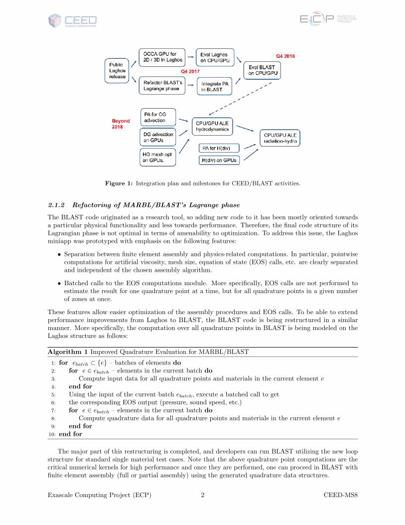
Figure 1 shows a detailed plan and timeline for integrating CEED technologies into BLAST, derived inclose collaboration between the CEED and BLAST teams. In this report we concentrate on the first threetasks that were planned for completion by the end of Q4 FY17. Details of Laghos, its recent improvements,and the related Open Concurrent Compute Abstraction (OCCA) GPU implementation efforts are discussedin Section 3.1. The refactoring of the BLAST Lagrange phase code is addressed in the next section.

As indicated in Figure 1, a main focus in FY18 will be the completion of the BLAST Lagrangian phaseoptimization, for both CPU and GPU performance. The exploration of different CPU and GPU optimizationtechniques in Laghos can make a big difference and will be invaluable in that regard, see e.g. Section 4.1in this report. Beyond FY18, the CEED efforts will target the optimization of the full ALE algorithm,which includes methods for Continuous Galerkin (CG) advection, Discontinuous Galerkin (DG) monotoneadvection and high-order mesh optimization. After these tasks, CEED will concentrate on optimizing theradiation-hydrodynamics module of BLAST, which requires GPU implementation of operations on the H(div)spaces, including partial assembly and matrix-free preconditioners for H(div) linear systems.

Exascale Computing Project (ECP) 1 CEED-MS8



Figure 1: Integration plan and milestones for CEED/BLAST activities.

2.1.2 Refactoring of MARBL/BLAST’s Lagrange phase

The BLAST code originated as a research tool, so adding new code to it has been mostly oriented towardsa particular physical functionality and less towards performance. Therefore, the final code structure of itsLagrangian phase is not optimal in terms of amenability to optimization. To address this issue, the Laghosminiapp was prototyped with emphasis on the following features:

• Separation between finite element assembly and physics-related computations. In particular, pointwisecomputations for artificial viscosity, mesh size, equation of state (EOS) calls, etc. are clearly separatedand independent of the chosen assembly algorithm.

• Batched calls to the EOS computations module. More specifically, EOS calls are not performed toestimate the result for one quadrature point at a time, but for all quadrature points in a given numberof zones at once.

These features allow easier optimization of the assembly procedures and EOS calls. To be able to extendperformance improvements from Laghos to BLAST, the BLAST code is being restructured in a similarmanner. More specifically, the computation over all quadrature points in BLAST is being modeled on theLaghos structure as follows:

Algorithm 1 Improved Quadrature Evaluation for MARBL/BLAST

1: for ebatch ⊂ {e} – batches of elements do2: for e ∈ ebatch – elements in the current batch do3: Compute input data for all quadrature points and materials in the current element e4: end for5: Using the input of the current batch ebatch, execute a batched call to get6: the corresponding EOS output (pressure, sound speed, etc.)7: for e ∈ ebatch – elements in the current batch do8: Compute quadrature data for all quadrature points and materials in the current element e9: end for

10: end for

The major part of this restructuring is completed, and developers can run BLAST utilizing the new loopstructure for standard single material test cases. Note that the above quadrature point computations are thecritical numerical kernels for high performance and once they are performed, one can proceed in BLAST withfinite element assembly (full or partial assembly) using the generated quadrature data structures.


2.2 ExaSMR

The ExaSMR project is focused on the exascale application of single and coupled MC and CFD physics.The application development objective is to optimize these applications for exascale execution of full coresimulations. A CEED milestone, joint with ExaSMR, in Q4 FY17 focuses on initial GPU porting of Nek5000for assembly-level simulations, provided with baseline performance. We report a successful GPU porting ofNek5000 with validation and demonstrate baseline performance for two benchmark problems: a subchannelproblem (single-rod) to assess intranode performance and a larger full assembly problem with 17× 17 rods,shown in Figure 2.

Figure 2: ExaSMR spectral element hexahedral meshes for subchannel and fullassembly systems with 2× 2 (left) and 17× 17 (right) rods.

2.2.1 Nek5000 GPU Implementation

The initial GPU implementation is based on OpenACC pragmas and provides a basis for future accelerator-based development for Nek5000, extended from previous works[1, 2]. The principal focus has been onthe linear system solves that constitute 70–80% of typical production runtimes. The port includes thefull spectral element multigrid preconditioner and uses an extension of the Nek gather-scatter librarygslib, http://github.com/gslib, that supports local (on-device) gather-scatters to minimize off-devicecommunication.

We use OpenACC as a strategy for porting Nek5000 to GPU because of the relative ease of the pragma-based porting. OpenACC is a directive-based HPC parallel programming model, using host-directed executionwith an attached accelerator device. The compiler maps the compute and data regions specified by theOpenACC directives to GPUs for higher performance. In contrast to other low-level GPU programming, suchas CUDA and OpenCL, where more explicit compute and data management is necessary, porting of legacyCPU-based applications with OpenACC does not require significant structural changes in the original code,which allows considerable simplification and productivity improvement when hybridizing existing applications.

Before starting the Nek5000 time-advancement, each CPU executes data movement from the host CPUmemory to GPU memory, and the majority of the computation is performed on GPUs during each time step.Within each step, the host CPU transfers GPU results back to the host when processing boundary conditionsand the coarse-grid solver, neither of which are compute intensive. User-prescribed forcing functions andmaterial properties are also implemented on the host. Inter-element (GPU-GPU) data exchanges are effectedusing GPU-direct communication, when available, or through a device-to-host transfer followed by MPI. Bothmodes are supported by gslib, which is called directly from the GPU.

While the directive-based approach of OpenACC greatly simplifies programming, it does not provide theperformance flexibility of CUDA or OpenCL. For example, both CUDA and OpenCL provide fine-grained


http://github.com/gslib

Figure 3: Nek5000 fully GPU-ported runs with validation for different boundaryconditions for 3D eddy simulations, demonstrating spectral convergence as in-creasing N = 3, 5, 7, 9, 11, 13, 15 with E = 4× 4× 3 at time step 50; A single-rodmesh with N = 7 and E = 2560 demonstrating pressure solve iteration counts for1000 step runs with validated results agreeing up to 12–14 digits between CPUvs. GPU.

synchronization primitives, such as thread synchronization and atomic operations, whereas OpenACC doesnot. Efficient implementations of applications may depend on the availability of software-managed on-chipmemory, which can be used directly in CUDA and OpenCL, but not in OpenACC. These differences mayprevent full use of the available architectural resources, potentially resulting in inferior performance whencompared to highly tuned CUDA and OpenCL code. As a future strategy, we investigate highly optimizedkernels based on the OCCA abstraction, which can produce low-level CUDA, OpenCL, or OpenMP codewithin a unified flexible framework. The potential for high performance using this strategy is discussed indetail in Section 4.1.

2.2.2 Nek5000 GPU/CPU Verification and Performance on ExaSMR Tests

The Nek5000 port has been developed on single-GPU platforms at ANL and extensively tested in multi-GPUsettings on Titan and Summit-Dev at ORNL. Verification has included extensive comparisons to analyticalsolutions and to the baseline Nek5000 code for single- and multi-rod simulations relevant to the ExaSMRapplication. Figure 3 demonstrates verification of the GPU port for analytical solutions (3D extensionsof Nek5000’s eddy case) for the Navier-Stokes equations with Dirichlet, Neumann and mixed boundary


conditions. Spectral (exponential) convergence is observed at time step 50 with increasing N for a mesh withE = 4 × 4 × 3 elements. In Figure 3, we also demonstrate that the pressure solve iteration counts are inagreement between the GPU and CPU versions for 1000 time steps of a single-rod mesh with polynomialorder N = 7 and E = 2, 560 elements. In all cases, the GPU version agrees to within 12–14 digits with thestandard Nek5000 baseline.

Table 1: Nek5000 single-rod run timings on P100 vs. Intel Xeon GHz (JLSEneddy/maud).

single-rodComparison

1 GPU 16 CPU Corestotal elapsed time 1.64117E+01 sec 1.73326E+01 sectotal solver time incl. I/O 1.06078E+01 sec 1.18436E+01 sectime/timestep 2.12157E+00 sec 2.36871E+00 sec

Figure 4: Nek5000 performance on SummitDev, Titan, and Theta.

Performance tuning of the GPU port is continuing on the platforms listed in Table 2. Current peakperformance for the OpenACC kernels is a few hundred GFLOPS on an NVIDIA P100 (ALCF JLSE maud)demonstrating 90% of the speed of 16 Intel Xeon 2.2 GHz cores (ALCF JLSE), as shown in Table 1. Bycontrast, highly-tuned OCCA-driven CUDA kernels are exceeding 1 TFLOPS on the same GPU. (See Section4.1). The next round of Nek5000-GPU development will involve using the OCCA-based kernels beingdeveloped by the group of Warburton at Virginia Tech under CEED.

Initial GPU+MPI simulation results with Nek5000 are shown in Figure 4, along with several CPU+MPIresults. At this point, the GPU results are still slower than the parallel CPU runs, which have benefited fromdecades of development and tuning. We have identified several areas that need to be addressed in the Nek5000GPU port which include: reductions in the number of host-device transfers, functional implementationof essentially all compute-intensive kernels (e.g., GPU-based advection is not properly functioning at thismoment), and running sufficiently large (local) problems to keep each GPU busy and amortize MPI overhead.From Figure 4 (left), it is clear that there is not enough work to saturate the (current) GPU implementationin the single-rod case. (This latter point has been explored in the context of our earlier work with NekCEMon Titan.) Technical issues have kept the GPU version from functioning for the 17x17 rod case on SummitDevin GPU mode, so timings are not yet available for the larger cases.

In addition to the holistic approach of having a functional GPU-based version of Nek5000 that is consistent


(to very high precision) with the baseline version, we have pursued development and tests of highly performantkernels with several implementations of OpenACC. For example, one of the most important is the Poissonkernel (BP3.5, described in Section 4.1). Working with NVIDIA and ORNL engineers, we were able to get∼200-300 GFLOPS for this kernel (GPU only, no MPI). A key factor in boosting performance was to lock inarray dimensions at compile time, rather than leaving the (leading) array dimensions as run-time variables.This change was straightforward in Nek5000 because the polynomial order is fixed at compile time. For somekernels, this change yielded as much as a six-fold performance gain.

Despite these gains, it became clear that OpenACC might not be able to deliver the high fraction ofpeak that we are seeking on the GPU and some approach affording more fine-grained control is in order.Our choice will be OCCA, because it does not lock us into vendor-specific code (e.g., CUDA). Even withsuch fine-grained control, high-performance is not automatic. As described in Section 4.1, many iterations ofdevelopment were required to yield TFLOPS/s performance.

2.3 Other ECP Applications

2.3.1 Urban

Urbanization is one of the great challenges and opportunities of this century, inextricably tied to globalchallenges ranging from climate change to sustainable use of energy and other natural resources, and frompersonal health and safety to accelerating innovation in metropolitan communities. Enabling science- andevidence-based urban design, policy and operation will require discovery, characterization and quantificationof the inter-dependencies between major metropolitan sectors. Central to these inter-dependencies is humanactivity—decisions driven by social and economic factors—underpinning much of the use and development ofcities.

The Urban team, in collaboration with the CEED team, explore the coupling of LES and building energydemand models, considering the building envelope as the boundary while current LES models operate atresolutions too coarse for use to examine the heat flow in urban canyons and how building designs and otherfactors related to urban form impact that flow. Using Nek5000 as the LES code, we have ongoing scopingsimulations with grid sizes ranging from 1 to 100 meters square buildings, evaluating data flow characteristicsand mesh requirements particularly with respect to further coupling with the building energy models thatcan be efficiently marched in time. In order to overcome the vast disparity of spatio-temporal scales for atarget exascale simulation, we plan to mesh a sufficiently small but representative urban flow domain andcompute a reference solution with maximum fidelity and resolution possible at a current leadership platforms.Then we can use this simulation to compare with a faster-turn-around but reduced fidelity models that canbe further applied to larger urban landscape geometries.

As a first step toward acquiring the reference simulation, we have obtained preliminary simulation resultswith Nek5000 for airflow around the Lake Point Tower building geometry. Figure 5 shows velocity magnitudeslices for a case where wind blowing from the lake shows regions of large sheer and velocity gradients whichrequire further mesh improvements for an efficient computation at scale.

On a separate note relevant to target exascale simulations, the CEED team’s effort in FY17 Q4 includedsignificant performance improvement in I/O kernels, supporting large element counts (> 15M elements).

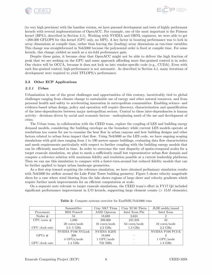
Table 2: Compute systems overview for ExaSMR/Nek5000 runs

SummitDev Cray XK7 Titan Cray XC40 Theta JLSE neddy/maud

Processors IBM Power9 AMD Opteron Intel Xeon Phi Intel Xeon

Nodes # 54 18,688 3,624 2

CPU cores # 1,080 299,008 231,935 3220 cores/node 16 cores/node 64 cores/node 16 cores/node

CPU clock rate 2.5–5 GHz 2.2 GHz 1.3 GHz 2.2 GHz

NVIDIA P100 NVLink NVIDIA K20X NVIDIA P100 PCI-EGPUs # 208 18,688 – 2

4 GPUs/node 1 GPU/node – 1 GPU/nodeGPU clock rate 1.4 GHz 732 MHz – 1.3 GHz


Figure 5: Preliminary LES results for a reference dataset of the flow over asmall but representative landscape that includes the Lake Point Tower buildinggeometry.

Further improvements and testing is ongoing.

2.3.2 ACME

The ACME-MMF project is developing a super-parameterized configuration of the DOE ACME Earth SystemModel, targeting the super-parametrization subcomponent modeling and simulations on future exascalearchitectures. One of the most compute expensive subcomponent includes the atmosphere dynamical core,HOMME, that is based on the spectral-element method, and ACME-MMF team plans to benefit by advancesdeveloped by the CEED project in high-order-element-based methods to achieve exascale performance andperformance portability. Ongoing discussion identifying potential collaboration between ACME-MMF andCEED team include the following.

• Flow on a manifold. One of the most effective ways of dealing with spherical geometry in atmospheremodels, and the approach taken by HOMME, is to use a 2D+1 approach. This approach separates thehorizontal (surface of the sphere directions) from the vertical/radial direction and uses a 2D spectralelement discretization of spherical shells, coupled to a 1D finite-difference discretization in the vertical.For a spectral element library, the key requirements are the ability to include metric terms (curvature)in the map from the physical element to the reference element while the physical element is a 2Delement that lives in R3, while the reference element lives in R2.

• For efficiency, with a 2D+1 approach, ideally the vertical direction should be included as an array indexfor all state and field variables within each element, but not included with the various metric terms andhorizontal derivatives that do not depend on the vertical coordinate. Vertical operators are relativelystraightforward and could be implemented in the application or in the CEED library.


• Support for general curvilinear maps where the most natural map for spherical geometry is projectionfrom the center of the sphere, which is non-orthogonal.

• Support efficient kernels for horizontal differential operators: HOMME relies on div, grad, and curloperators in strong form (nodal values), separate routines for their integrated-by-parts form and anintegrated-by-parts scalar Laplacian and vector Laplacian.

2.3.3 ExaAM

The ECP Exascale Additive Manufacturing Application Project (ExaAM) couples multi-physics and multi-codes in an effort to use exascale computing to enable better qualification of additive manufacturing(AM) built parts. Fundamentally, this means coupling microsctructure development and local propertyanalysis with process simulation. The ExaAM code with the physics required for the local property analysisis an export controlled code, and with the goal of creating an open source software platform for AMsimulation, the ExaAM team explored the space of mini and proxy apps, and none were found suitable.The ExaAM team decided to create a new miniapp specifically for local property analysis in collaborationwith the CEED team. The initial release (ExaConstit) is planned to remain ExaAM’s miniapp for thisapplication area and will become the foundation of a prototype application as required physics is addedfor local property analysis for AM materials. Significant integration between the ExaAM and CEEDECP activities is planned during this process. The new ExaConstit miniapp is currently available athttps://github.com/mfem/mfem/tree/exaconstit-dev/miniapps/exaconstit and, after approval, willbe part of the MFEM release on GitHub.

2.3.4 GEOS

The ECP Subsurface Simulator application (ADSE05) utilizes LLNL’s GEOS code to model large scaledeformation and flow, and LBNL’s Chombo-Crunch code to pore scale flow and geochemistry in an effort tosolve reservoir scale problems that also require direct simulation of pore scale physics. GEOS is a generalpurpose simulation framework that facilitates various numerical schemes such as the Finite Element Methodand the Finite Volume Method, and has had success modeling the coupled flow, deformation, and fractureinvolved in the hydraulic stimulation of a tight shale reservoir. The approach to modeling fracture throughmesh topology change has distinct advantages but also carries limitations, such as difficulties utilizing higherorder discretizations. Although CEED is primarily an effort focused on higher order methods, the organizationof various computational kernels that arise from the Finite Element Methods into a collection is potentiallyuseful for any finite element code. As such, the GEOS-ECP team intends to utilize the CEED kernel library toorganize a collection of low order super-element kernels that take advantage of the reduced memory demandsof a higher order element while maintaining the topological flexibility of a low order discretization. TheCEED and GEOS teams are also exploring the possibility of developing a simple MFEM-based miniapp forsubsurface flow.

2.3.5 Combustion

DNS and LES of combustion problems is of major importance to the DOE mission. In collaboration withthe Energy Systems Division at Argonne and Aerothermochemistry and Combustion Systems Laboratory atETH Zurich, we have extended the arbitrary Lagrangian Eulerian (ALE) formulation in Nek5000 to supportcharacteristics-based time-stepping that allows simulations to exceed standard Courant-Friedrichs-Lewy (CFL)stability constraints. In internal combustion simulations, the CFL constraint can be quite limiting duringvalve-open events, when the highest velocities are flowing through the intake or exhaust valve regions whichtypically have very fine mesh spacing. The characteristics scheme decouples advection from the pressure andviscous solves of the associated unsteady Stokes problem. Advection is effected through small CFL-stabletime steps with no expensive pressure solves. The linear Stokes problems can be advanced with a time stepthat is an order of magnitude larger than the CFL-limited step size. Accounting for all the overhead, the netsavings observed in recent (cold-flow) engine simulations is a factor of 3 to 4.


https://github.com/mfem/mfem/tree/exaconstit-dev/miniapps/exaconstit

2.4 ECP Application Assessment

2.4.1 Nek5000 Full Application Weak and Strong Scaling

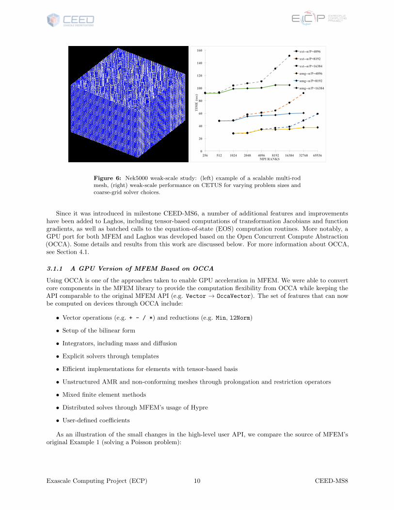
As part of the ECP Application Assessment Project with Kenny Roche (PNNL), we have performed aweak-scale study of Nek5000 on multipin geometries similar to those required for ExaSMR, as shown inFigure 6 (left). To simplify this study for a relatively large weak/strong-scale study, which involves generationof several meshes to cover the range of interest, we have eliminated the solid center of the pins in thismulti-rod test case and thus focus only on the hydro plus thermal advection. (That is, we ignore diffusionin the additional elements that would make up the solid.) This simplification permits more transparentperformance analysis across a wide range of processor counts and problem sizes because the algorithm ismore homogeneous. Given that hydrodynamics typically dominates the solution time, this simplification canbe made safely without undue compromise of the model problem’s fidelity to the target exascale application.

The baseline mesh for single-rod consisted of Exy = 256 elements in the x − y plane, extrude in the zdirection to yield E = Exy × Ez = 2560 elements. (Thus, Ez = 10.) For this larger study, we use anywhereup to E = 524288 elements, which can be realized through a combination of multiple pins and multiple layersin the axial flow direction. The 3D meshes are a tensor product of the 256-element 2D unit cell with Ez slabsin the z direction, and Cx × Cy cells in the x and y directions, respectively. In the present study, we fix thepolynomial order to N = 7, which implies for the largest case, of E = 219, we have n ≈ EN3 = 179.8 millionpoints. Note that we would expect a problem of this size to strong scale out to about P = 100, 000 on BG/Q[3], where there are about n/P=2000 points per core. On other machines, strong-scale fall-off will probablybe at P < 100, 000.

Figure 6 (right) shows the weak-scale performance on BG/Q (Cetus) for several values of n/P . Twofamilies of curves are shown. One uses the Nek5000 default fast direct XXT -solver [4] that is used forstandard small-scale production runs. The other uses algebraic multigrid [5] for the coarse-grid solver. XXT

is highly effective up to about 100,000 elements (in accord with analysis in [4], but AMG is superior beyondthat point).

2.4.2 NekBench Utilities for Scaling Studies

The Nekbench repository https://github.com/thilinarmtb/NekBench provides scripts for benchmarkingNek5000. The user provides ranges for the important parameters (e.g., processor counts and local problemsize ranges) and a test type (e.g., scaling or ping-pong test). Nekbench will run the given test in the givenparameter space using a Nek5000 case file, which is also given by the user (in the ping-pong tests, the casefile is optional). Nekbench is written using bash scripting language and runs any Unix-like operating systemthat supports bash. It has been successfully tested on Linux laptops/desktops, ALCF Theta, NERSC Cori(KNL and Haswell), and NERSC Edison machines for scaling tests.

Planned extensions for Nekbench include adding more machine types like Cetus, additional support forthe ping-pong test type, and automated plot generation (e.g., scaling study graphs) for each test run.

3. MINIAPPS

3.1 Laghos

Laghos (LAGrangian High-Order Solver) is a new miniapp developed in CEED that solves the time-dependentEuler equations of compressible gas dynamics in a moving Lagrangian frame using unstructured high-orderfinite element spatial discretization and explicit high-order time-stepping. In CEED, Laghos serves as a proxyfor a sub-component of the MARBL/LLNLApp application.

Laghos captures the basic structure and user interface of many other compressible shock hydrocodes,including the BLAST code at LLNL. The miniapp is built on top of a general discretization library (MFEM),thus separating the pointwise physics from finite element and meshing concerns. It exposes the principalcomputational kernels of explicit time-dependent shock-capturing compressible flow, including the FLOP-intensive definition of artificial viscosity at quadrature points. The implementation is based on the numericalalgorithm from [6]. The miniapp is available at https://github.com/ceed/Laghos.


https://github.com/thilinarmtb/NekBench

https://github.com/ceed/Laghos

0

20

40

60

80

100

120

140

160

256 512 1024 2048 4096 8192 16384 32768 65536

TIM

E (s

ec)

MPI RANKS

xxt--n/P=4096

xxt--n/P=8192

xxt--n/P=16384

amg--n/P=4096

amg--n/P=8192

amg--n/P=16384

Figure 6: Nek5000 weak-scale study: (left) example of a scalable multi-rodmesh, (right) weak-scale performance on CETUS for varying problem sizes andcoarse-grid solver choices.

Since it was introduced in milestone CEED-MS6, a number of additional features and improvementshave been added to Laghos, including tensor-based computations of transformation Jacobians and functiongradients, as well as batched calls to the equation-of-state (EOS) computation routines. More notably, aGPU port for both MFEM and Laghos was developed based on the Open Concurrent Compute Abstraction(OCCA). Some details and results from this work are discussed below. For more information about OCCA,see Section 4.1.

3.1.1 A GPU Version of MFEM Based on OCCA

Using OCCA is one of the approaches taken to enable GPU acceleration in MFEM. We were able to convertcore components in the MFEM library to provide the computation flexibility from OCCA while keeping theAPI comparable to the original MFEM API (e.g. Vector → OccaVector). The set of features that can nowbe computed on devices through OCCA include:

• Vector operations (e.g. + - / *) and reductions (e.g. Min, l2Norm)

• Setup of the bilinear form

• Integrators, including mass and diffusion

• Explicit solvers through templates

• Efficient implementations for elements with tensor-based basis

• Unstructured AMR and non-conforming meshes through prolongation and restriction operators

• Mixed finite element methods

• Distributed solves through MFEM’s usage of Hypre

• User-defined coefficients

As an illustration of the small changes in the high-level user API, we compare the source of MFEM’soriginal Example 1 (solving a Poisson problem):


FiniteElementSpace *fespace = new FiniteElementSpace(mesh , fec);

Array <int > ess_tdof_list;

Vector x, b;

...

Operator *A;

Vector B, X;

BilinearForm *a = new BilinearForm(ofespace );

a->AddDomainIntegrator(new DiffusionIntegrator (1.0));

a->FormLinearSystem(ess_tdof_list , x, b, A, X, B);

CG(*A, B, X, 1, 500, 1e-12, 0.0);

with the OCCA-ported version:

occa:: setDevice("mode: CUDA , deviceID: 0")

OccaFiniteElementSpace *fespace = new OccaFiniteElementSpace(mesh , fec);

Array <int > ess_tdof_list;

OccaVector x, b;

...

Operator *A;

OccaVector B, X;

OccaBilinearForm *a = new OccaBilinearForm(ofespace );

a->AddDomainIntegrator(new OccaDiffusionIntegrator (1.0));

a->FormLinearSystem(ess_tdof_list , x, b, A, X, B);

CG(*A, B, X, 1, 500, 1e-12, 0.0);

In raw numbers, the OCCA port of MFEM required a change of 13k lines added and 1k lines removed, tobe compared with the initial 120k lines of code in the MFEM library. Using sloccount, we see a change from93k lines to 100k lines which include 2.5k lines from OCCA kernels. We were able to reduce the amount of codeneeded by leveraging OCCA’s just in time (JIT) kernel compilation and templating. For example, OccaVectorincludes 25 methods computed in OCCA with a 2-5 line kernels such as the OccaVector::operator +=

kernel.

makeCustomBuilder("vector_op_add", "v0[i] += c0;");

3.1.2 Laghos on OCCA

Laghos is the first miniapp to make use of the MFEM+OCCA API. Every time step of the computationfound in this miniapp contains three major stages:

• Inversion of a global mass operator based on the H1 space. This operation involves applications of themass operator for every CG iteration.

• Application of a force operator, using both H1 and L2 spaces. The force operator is applied two timesper time step.

• Computation of physical stresses at all quadrature points.


We leveraged the OccaMassIntegrator that was already ported in MFEM, but created custom kernelsfor the force operator and quadrature point updates. For the force operator and stress updates, distinctkernels were written for combinations of 2D and 3D elements, as well as for CPU and GPU architectures.

Below, in Figures 7–12, we present a preliminary comparison between the performance of the CPU Laghoscode (original CPU version without OCCA) and the OCCA GPU implementation. For the CPU case, we testboth the full and partial assembly options, denoted by FA and PA in the figures. We perform one time stepof the Taylor-Green test case, which does not involve any discontinuities in the solution fields (test on theSedov blast problem will be performed soon). Execution rates for all three major stages are presented, in 2Dand 3D. Each label denotes the finite element spaces used for the corresponding result set, e.g., Q4Q3 meanscontinuous kinematic space of type Q4 and discontinuous thermodynamic set of type Q3 on each cell.

All tests were performed on the Ray machine at LLNL, where each node has two IBM Power8 CPUs, eachwith 10 cores with 8 threads per core, and 4 Tesla P100 GPUs. All CPU runs were performed on one nodeusing 16 and 64 MPI tasks in 2D and 3D, respectively. The GPU calculations use only one of the GPUs.

In Figures 7 and 8 we see that the CPU PA option is more beneficial than the CPU FA for orders 3 andabove. It is important to keep in mind that the CPU FA applies a precomputed sparse matrix without anyassembly operations (they are not included in the timing). The OCCA code is currently slower than theCPU partial assembly but, based on the BP2 results in CEED-MS6, we beleive that this performance can beimproved significantly.

Figures 9 and 10 are related only to the application of the force operator; the computation of the dataneeded to form it is not included in the timing. The OCCA version is the best choice, performing better thanthe PA for every order and achieving about 800 MDOFs. Focusing on Figure 9, we see that we get about anorder of magnitude improvement from a better algorithm (PA vs FA) and another order from the hardware(going from 16 cores to 1 GPU).

Figures 11 and 12 show that the OCCA code is also the best option for quadrature-based computations,exploiting the fact that these calculations do not involve any communication.

Figures 13 and 14 compare the total execution time of the three main kernels for the FA and PA options.The show that PA is the clearly preferred options for all orders except order 1 in 3D.

Figure 7: Laghos: 2D inversion of the global mass operator.

3.2 Nekbone

3.2.1 Introduction and Algorithm

Nekbone is a lightweight subset of Nek5000 that is intended to mimic the essential computational complexityof Nek5000, relevant to large eddy simulation (LES) and direct numerical simulation (DNS) of turbulence incomplex domains, in relatively few lines of code. It allows software and hardware developers to understandthe basic structure and computational costs of Nek5000 over a broad spectrum of architectures ranging fromsoftware-based simulators running at one ten-thousandth the speed of current processors to exascale platformsrunning millions of times faster than single-core platforms. Nekbone has weak-scaled to 6 million MPI rankson the Blue Gene/Q Sequoia at LLNL while Nek5000 has strong-scaled to over a million ranks on the BlueGene/Q Mira at ANL. Nekbone provides flexibility to adapt new programming approaches for scalabilityand performance studies on a variety of platforms without having to understand all the features of Nek5000,


Figure 8: Laghos: 3D inversion of the global mass operator.

Figure 9: Laghos: 2D application of the force operator.

Figure 10: Laghos: 3D application of the force operator.

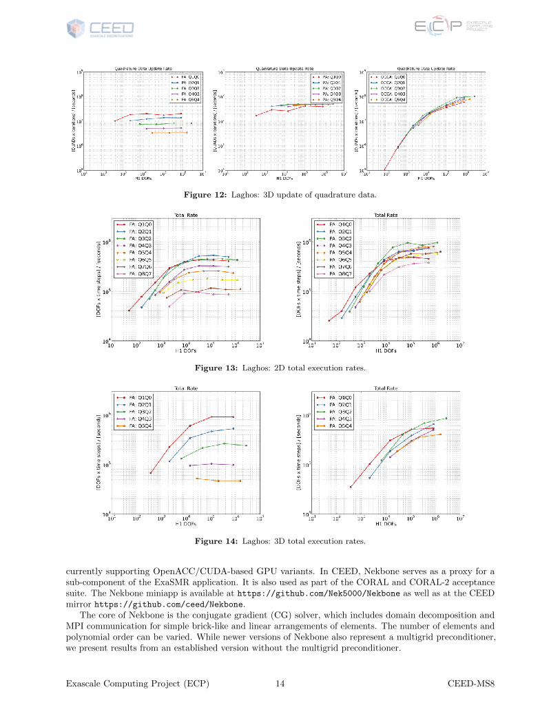
Figure 11: Laghos: 2D update of quadrature data.


Figure 12: Laghos: 3D update of quadrature data.

Figure 13: Laghos: 2D total execution rates.

Figure 14: Laghos: 3D total execution rates.

currently supporting OpenACC/CUDA-based GPU variants. In CEED, Nekbone serves as a proxy for asub-component of the ExaSMR application. It is also used as part of the CORAL and CORAL-2 acceptancesuite. The Nekbone miniapp is available at https://github.com/Nek5000/Nekbone as well as at the CEEDmirror https://github.com/ceed/Nekbone.

The core of Nekbone is the conjugate gradient (CG) solver, which includes domain decomposition andMPI communication for simple brick-like and linear arrangements of elements. The number of elements andpolynomial order can be varied. While newer versions of Nekbone also represent a multigrid preconditioner,we present results from an established version without the multigrid preconditioner.


https://github.com/Nek5000/Nekbone

https://github.com/ceed/Nekbone

Table 3: Performance model of CPU Nekbone

Subroutine DP Loads DP Stores DP Ops q

glsc3 3n 0 3n 0.125add2s1 2n n 2n 0.083

local grad3 n 0 6nnx 0.75nxwr ws wt 6n 0 15n 0.26

local grad3 t 0 n 6nnx + 2n 0.75 + 0.25nxadd2s2 2n n 2n 0.083

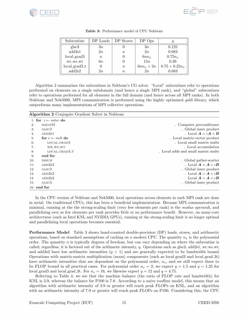
Algorithm 2 summarizes the subroutines in Nekbone’s CG solver. “Local” subroutines refer to operationsperformed on elements on a single subdomain (and hence a single MPI rank), and “global” subroutinesrefer to operations performed for all elements in the full domain (and hence across all MPI ranks). In bothNekbone and Nek5000, MPI communication is performed using the highly optimized gslib library, whichoutperforms many implementations of MPI collective operations.

Algorithm 2 Conjugate Gradient Solver in Nekbone

1: for i← niter do2: solveM . Computer preconditioner3: glsc3 . Global inner product4: add2s1 . Local A = cA + B5: for e← nelt do . Local matrix-vector product6: local grad3 . Local small matrix mults7: wr ws wt . Local accumulation8: local grad3 t . Local adds and small matrix mults9: end for

10: dssum . Global gather-scatter11: add2s2 . Local A = A + cB12: glsc3 . Global inner product13: add2s2 . Local A = A + cB14: add2s2 . Local A = A + cB15: glsc3 . Global inner product

16: end for

In the CPU version of Nekbone and Nek5000, local operations across elements in each MPI rank are donein serial. On traditional CPUs, this has been a beneficial implementation. Because MPI communication isminimal, running at the the strong-scaling limit (very few elements per rank) is the modus operandi, andparallelizing over so few elements per rank provides little or no performance benefit. However, on many-corearchitectures (such as Intel KNL and NVIDIA GPUs), running at the strong-scaling limit is no longer optimaland parallelizing local operations becomes essential.

Performance Model Table 3 shows hand-counted double-precision (DP) loads, stores, and arithmeticoperations, based on standard assumptions of caching on a modern CPU. The quantity nx is the polynomialorder. The quantity n is typically degrees of freedom, but can vary depending on where the subroutine iscalled; regardless, it is factored out of the arithmetic intensity, q. Operations such as glsc3, add2s1, wr ws wt,and add2s2 have low arithmetic intensities (q < 1) and are generally expected to be bandwidth bound.Operations with matrix-matrix multiplication (mxm) components (such as local grad3 and local grad 3t)have arithmetic intensities that are dependent on the polynomial order, nx, and we still expect these tobe FLOP bound in all practical cases. For polynomial order nx = 2, we expect q = 1.5 and q = 1.25 forlocal grad3 and local grad 3t. For nx = 16, we likewise expect q = 12 and q = 4.75.

Referring to Table 4, we see that the machine balance (the ratio of FLOP rate and bandwidth) forKNL is 3.9, whereas the balance for P100 is 7.8. According to a naive roofline model, this means that analgorithm with arithmetic intensity of 3.9 or greater will reach peak FLOPs on KNL, and an algorithmwith an arithmetic intensity of 7.9 or greater will reach peak FLOPs on P100. Considering this, the CPU


performance model in Table 5 demonstrates that in general, mxm operations (local grad3 and local grad 3t)will only approach peak FLOP/s for higher polynomial orders, since the arithmetic intensity of mxm isproportional to polynomial order. Finally, this model demonstrates that, on GPU compared to KNL, thepolynomial must be higher to reach peak on-node FLOP/s.

This performance model alone does not offer insight into performance with respect to number of elementsper node. The following tests provide some insight into this question for the particular case of KNL usingOpenMP. Figure 15 shows the CG solve time with respect to degrees of freedom per node for 100-timestepproblems with polynomial order 7 on an Intel KNL (one node of Theta). The implementations include:

• Serial/OpenMP execution on KNL

• Serial/OpenMP on KNL using a DGEMMs expressed as unrolled loops

• Serial/OpenMP on KNL using vendor-optimized libxsmm for matrix-vector products

From Figure 15, we see that at least n = 220 gridpoints are required before a single node of KNL, running 64OpenMP threads, demonstrates linear scaling. Below this number, the runtime is flat, i.e., not decreasing withreduced problem size, because the resources are not being fully utilized. If we denote by P the number of threads(or MPI ranks in the all-MPI case), this value of n/P = 16384 is consistent with but larger than what is foundto be required on BG/Q, where the performance roll-off is (conservatively) at n/P ≈ 8000 [3]. More detailson this analysis are presented here: https://asc.llnl.gov/DOE-COE-Mtg-2016/talks/1-13_Parker.pdf.

3.3 CORAL-2 Benchmarks and Vendor Interactions

The CEED miniapps are designed to be used as CEED’s main vehicle in a variety of co-design activities withECP vendors, software technologies projects and external partners.

A major highlight in this direction is that two of the CEED high-order miniapps: Nekbone, and thenewly developed Laghos, were selected to be part of the CORAL-2 procurement benchmark suite, seehttps://asc.llnl.gov/coral-2-benchmarks. In addition, Nekbone, Laghos and HPGMG are now part ofthe proxy app list https://exascaleproject.github.io/proxy-apps/all-apps maintained by the ECPProxy App project.

The CEED team has been using the Nekbone and Laghos miniapps, as well as the CEED benchmarks, http://ceed.exascaleproject.org/bps to engage researchers in Intel, Cray and AMD, as well as the internationalhigh-order community. We sent multiple representatives to Intel’s first hackathon in Hudson, MA (where weran kernels from these miniapps on their simulators) and will be represented in all of the Cray, Intel and AMDdeep-dives coming up in October 2017. External researchers from the deal.ii project have picked up and runour proposed bake-off problems (BPs), see https://github.com/kronbichler/ceed_benchmarks_dealii.

Table 4: Comparison of KNL and P100 Statistics

Metric KNL P100

Cores / SMX 64 56SIMD DP Width 8 32

Clock Speed [GHz] 1.1 1.3Peak f32 [TFLOP/s] 4.5 9.3Peak f64 [TFLOP/s] 2.3 4.7

Peak DGEMM [TFLOP/s] 1.9 4.5Memory (IPM) [GB] 16 16

IPM Bandwidth [GB/s] 600 732STREAM Bandwidth [GB/s] 488 574

L1 Cache per core / SMX [KB] 32(D), 32(I) 64L2 Cache [MB] 32 4

TDP[W] 215 250


https://asc.llnl.gov/DOE-COE-Mtg-2016/talks/1-13_Parker.pdf

https://asc.llnl.gov/coral-2-benchmarks

https://exascaleproject.github.io/proxy-apps/all-apps

http://ceed.exascaleproject.org/bps

http://ceed.exascaleproject.org/bps

https://github.com/kronbichler/ceed_benchmarks_dealii

Table 5: Performance Analysis of Nekbone on KNL

Subroutine Time (s) % Solve time BW (GB/s) % Peak BW GFLOP/s % Peak GFLOP/s

glsc3 1.56E-1 20.2 351.2 72 43.9wrwswt 1.28E-1 16.5 314.1 64 98.1add2s2 1.23E-2 16.02 480.3 98 40.0

local grad3 t 1.09E-1 14.1 754.4 40gs op 8.89E-2 11.5

local grad3 8.31E-2 10.7 969.6 51add2s1 4.23E-2 5.4 475.6 97 39.6

Table 6: Performance Analysis of Nekbone on GPU

Subroutine Time (s) % Solve time BW (GB/s) % Peak BW GFLOP/s % Peak GFLOP/s

local grad3 3.35e-1 33.1 187.01 278.22 6+ wrwswt

local grad3 t 2.96e-1 29.3 85.04 272.00 6glsc3 9.23e-2 12.4 545.31 95 109.42

add2s2 1.09e-1 10.8 512.36 89 46.20gs op 5.56e-2 5.5

add2s1 3.61e-2 3.6 512.81 89 46.52

4. GPU PERFORMANCE OPTIMIZATION

4.1 OCCA

In this section, we analyze the implementation strategies for spectral element operators on GPUs. We usethree benchmark problems taken from the CEED benchmark suite that are representative for a wide class ofoperators arising in spectral and high-order finite element methods. While there is no doubt that the GPUsare good accelerators, designing code that uses the GPU to its full potential requires deeper understanding ofboth the problem and the hardware architecture. We guide the reader through the benchmark problems, thechallenges associated with each problem, and through the implementation details and fine-tuning of the code.using the Open Concurrent Compute Abstraction (OCCA) [7]. As a result of the code optimization process,our GPU code reaches an empirically defined memory roofline bounds for all benchmark problems.

The choice of OCCA for this initial exploration is motivated by the fact that it offers several importantadvantages in the context of CEED applications:

• It exposes all performance critical features of CUDA required for finite element calculations, allowing usto experiment with different kernel implementations and achieve CUDA-like performance (as illustratedin this section).

• It offers runtime compilation of compute kernels with JIT specialization and optimization, which isparticularly important for high-order methods where innermost loops have bounds depending on theorder.

• It allows developers to write kernels in a portable code language that is simple to understand

• Unifies and simplifies interacting with CUDA, OpenCL, and OpenMP backends.

• Can be called from both C++ (MFEM) and FORTRAN (Nek), and kernels can be shared betweenlanguages.

• It is lightweight and very portable ( 60k lines of C++) so it can be used only internally in CEED tools,without requiring changes in the application.

The rest of this section is organized as follows: in Section 4.2 we provide a review of past efforts inGPU optimization of key finite element kernels. Section 4.3 introduces the notation used in the benhcmark


Figure 15: Nekbone OpenMP results on a single node of Theta (KNL).

problems described in the follow-on sections as follows: in Section 4.4, we introduce the first benchmarkproblem (mass matrix multiplication, BP1.0) and discuss the implementation and optimization choices; inSection 4.5, we discuss the second benchmark problem (collocation differentiation, BP3.5); and in Section 4.6,we analyze the third benchmark problem (differentiation involving interpolation and projection operations,BP3). We conclude the section by summarizing the GPU results and discussing future work in Section 4.7.

All kernel tuning was performed on an NVIDIA P100 PCI-E 12GB model. The fact that OCCA exposesa sufficiently comprehensive amount of CUDA functionality, allows us to fine tune the benchmark kernels fornearly ideal performance when compared with an empirical roofline model.

4.2 Background in GPU Acceleration of Finite Element Computations

Even before the era of easily programmable, general-purpose Graphic Processing Units, GPUs have beenused to speed up finite element codes. As early as 2007, Goddeke had solved 2D elliptic PDEs using a clusterequipped with GPU accelerators [8, 9], and during the next ten years, there have been a lot advancements inimplementation strategies.

Research generally focuses on accelerating specific parts of the computation and various aspects of thethe solution process, such as global assembly or the solver. For example, Cecka et al [10] targets the globalassembly phase of the finite element method (FEM), and shows how to optimize this phase for the GPUexecution. Markall et al [11] also concentrates on the global assembly phase. The authors emphasize that thechoice of the most efficient algorithm strongly depends on the available hardware and selected programmingmodel. The authors consider both the GPU and the CPU hardware, and both OpenCL and CUDA parallelimplementation. Some authors argue that making the code portable between different threading systems(such as many-core and multi-core architectures) requires a high-level language, see Markall et al [12, 11].Other researchers focus mostly on the solver part; in the paper by Goddeke et al [13] the authors use GPUsto accelerate Navier-Stokes solver for (lid) driven cavity and laminar flow over cylinder.

Few authors target the entire FEM pipeline using a canonical problems, i.e., Fu et. al. [14] used ellipticHelmholtz problem to show how to port the code to the GPU. The paper discusses strategies for acceleratingCG and multigrid solver. Another class of papers are those devoted to the GPU implementation of finiteelement discontinuous Galerkin (FEM-DG) methods. In [15], Klockner et. al. applies FEM-DG to solvehyperbolic PDEs on the GPUs. The work is continued by Klockner and coauthors in [16], where the details ofimplementation are provided. Remacle et. al. [17] shows a finite element scheme for solving elliptic equationsfor unstructured all-hex meshes on the GPUs. The authors also analyze the performance of the scheme usingan off-the-shelf GPU. Chan et. al. [18] constructs similar analysis for wave equation using hybrid meshes.


The cost of the matrix-vector multiplication typically accounts for the highest cost of the elliptic FEMsolver; see the work of Remacle et. al. [17, Table 2, Table 3]. Several authors target optimizing just this partof the solution process. For example, in the papers by Dehnavi et. al. [19] and Grigoras et. al. [20] we finddetailed description of implementation strategies for the matrix-vector product. Also, in [17], Remacle et. al.put high emphasis on optimizing matrix-free matrix-vector multiplication.

We have also concentrated on tuning GPU implementation of matrix-vector products arising in the CGsolver for elliptic FEM. In our case, we perform this operation elementwise, and we never assemble the globalmatrix, which is known as matrix-free matvec in the literature. There are many reasons why this matrix-vectorproduct is not easy to optimize on the GPU. First, by design we must perform the matrix-vector product instages with thread synchronization in between, and synchronization is expensive on the GPU. Second, weneed to allocate additional memory to store the intermediate results. For higher-order polynomials, doing sois troublesome because of the limited size of the on-chip memory. Third, we load and store a lot of data,especially if using geometric factors. Fourth, interpolation to a different set of nodes means that we areaccessing memory in an irregular fashion, which might cause bank conflicts.

4.3 Notation

In this section, we use the following notation.

SymbolCode Math MeaningN N degree of the polynomial used in the interpolationNq Nq number of Gauss-Lobatto-Legendre (GLL) nodes in 1 dimension. Note:

Nq = N + 1Np Np number of nodes in an element: Np = N3

q

glNq NGLq number of Gauss-Jacobi (GJ) nodes in 1 dimension. Note: NGL

q = N + 2

gjNp NGLp number of Gauss-Jacobi nodes in an element. NGL

p =(NGL

q

)3I I (N + 1)×N interpolation matrix used to interpolate GLL nodes to GJ nodesD D (N + 1)× (N + 1) differentiation matrix used in BP1.0, see (3)gjD DGL (N + 2)× (N + 2) differentiation matrix, used in BP3.0

NElements Nel Number of elements in the mesh

While listing parallel pseudocode, we use OCCA notation

• The shared quantifier denotes shared memory; shared variables are shared among all threads in thesame thread block.

• The exclusive quantifier denotes a register variable; a register variable belongs to one and only onethread.

• The occaBarrier and barrier quantifiers are used to denote thread synchronization; the code afterthe barrier is executed only if all the threads have finished the computations preceding the barrier.

• occaUnroll or Unroll is used to denote loop unrolling.

To present our analysis and results, we use three benchmark problems that capture typical part ofmatrix-vector multiplication in FEM: interpolation, differentiation, and projection in various configurations.Our main focus here is on performance of these benchmark problems on the GPU. We discuss the choicesone can make for the implementation, including the choices for parallel structure, memory layout, and datastreaming.


4.4 BP1.0: Mass Matrix Multiplication

The first benchmark we consider consists of the matrix-vector product of a high-order finite-element massmatrix and corresponding vector.This operation is used in several kinds of implementations of finite elementoperators including, but not limited to, elliptic operators, projection operations, and some preconditioningstrategies. This problem serves as a good initial performance benchmark as it consists of a very simple localmatrix action. The operation also requires relatively little data transfers compared with more demandingdifferential operators which necessitates loading geometric factors from the elements.

4.4.1 BP1.0 Mathematical Formulation

Let us consider an unstructured mesh of a domain D into K hexahedral elements Dk, k = 1, . . . ,K such that

D =

K⋃k=1

Dk.

We construct a high-order finite element approximation of a function u on the domain D by forming apolynomial uk on each element Dk. We express the polynomial uk as a sum of basis interpolation polynomialsby mapping the element Dk to a reference element D defined to be the bi-unit cube:

D = {(r, s, t) : 1 ≤ r ≤ 1,−1 ≤ s ≤ 1,−1 ≤ t ≤ 1}.

We choose a polynomial basis on D by taking a tensor product of one-dimensional Lagrange interpolationpolynomials lj based on N + 1 Gauss-Lobatto-Legendre (GLL) nodes on the interval [−1, 1]. In this way wecan write the polynomial uk as

uk (r, s, t) =

N∑i=0

N∑j=0

N∑k=0

uknijkli (r) lj (s) lk (t) ,

wherenijk = i+ j(N + 1) + k(N + 1)2,

so that 0 ≤ nijk < Np = (N + 1)3. We encode a polynomial q as a vector q of its polynomial coefficients,i.e. q = [q0, q1, . . . , qNp ]T . Using this notation, we define the local element mass matrix Mk to satisfy thefollowing definition

vTMkq =

∫D

|Jk(r, s, t)|v(r, s, t)q(r, s, t) drdsdt.

where |Jk| is determinant of the Jacobian of the mapping from Dk to D, given by

Jk =

∂x∂r

∂x∂s

∂x∂t

∂y∂r

∂y∂s

∂y∂t

∂z∂r

∂z∂s

∂z∂t

.

We evaluate the integral in each dimension separately using a Nq node GL quadrature. We denote the

quadrature weights and nodes in the r dimension as {wa}a=Nq

a=1 and {ra}a=Nq

a=1 , respectively, and use ananalogous notation for the s and t dimensions. We then write

vTMkq =

Nq∑a=1

Nq∑b=1

Nq∑c=1

wawbwcJk(ra, sb, tc)v(ra, sb, tc)q(ra, sb, tc).

Since the numerical quadrature is performed on the GL quadrature nodes instead of the GLL interpolationnodes, we need to interpolate uk to the GL nodes first before performing the integration. We define theinterpolation operators Ir, Is, and It such that

Irqili(r) = li(rq),

Isqj lj(s) = lj(sq), (1)

Itqklk(t) = lk(tq),


for all i, j, k = 0, . . . , N and q = 0, . . . , Nq. Using these operators and letting q = li(r)lj(s)lk(t) andv = li′(r)lj′(s)lk′(t), we find

Mkni′j′k′ ,nijk

=

Nq∑a=1

Nq∑b=1

Nq∑c=1

wawbwcJk(ra, sb, tc)I

rai′I

sbj′I

tck′IraiI

sbjI

tck,

Using matrix notation, we can write the action of the local mass matrix concisely as

Mk = (It)T (Is)T (Ir)TWIrIsIt,

where W is a diagonal matrix of weights and geometric data, i.e. W has entries

Wnabc,nabc= wawbwcJ

k(ra, sb, tc).

Note that the interpolation operators Ir, Is, and It are the same matrix operator acting of different dimensions.Hence the action of the local mass matrix consists of seven matrix-vector operations. Interpolation fromthe GLL interpolation nodes to the GL quadrature nodes comprises three matrix-vector products while thequadrature summation comprises a single matrix-vector product. Finally, the projection back to the GLLnodes via the transpose interpolation operator comprises three matrix-vector products.

We assemble the global mass matrix operator M by concatenating each of the element local mass matricesto form a block diagonal operator on the global vector of solution coefficients. Doing so, we write the actionof the mass matrix M on a vector q as

w = Mq.

Due to its block-diagonal structure, the mass matrix operator can be applied in a matrix-free (element-wise)way and no communication is required between elements. We detail the full matrix-free action of the massmatrix in the pseudocode in Algorithm 3.

Algorithm 3 BP1.0: mass matrix multiplication

1: Data: (1) q, size Nel ·N3q ; (2) Interpolation matrix I, size NGL

q ×Nq; (3) weights, G, size NGLq ·NGL

q ·NGLq

2: Output: Mq, size Nel ·N3q × 1

3: for every element e do4: for c, a = 1, . . . Nq, j = 1, . . . , NGL

q do

5: q(e)cja =

∑Nq

b=1 Ijbq(e)cba . Interpolate in b direction

6: end for7: for c = 1, . . . Nq, i, j = 1, . . . , NGL

q do

8: q(e)cja =

∑Nq

a=1 Iiaq(e)cja . Interpolate in a direction

9: end for10: for k, i, j = 1, . . . , NGL

q do

11: q(e)kji = G

(e)kji

∑Nq

c=1 Ikcq(e)cji . Interpolate in c direction, integrate

12: end for . Scale by Jacobian and integration weights13: for k, i = 1, . . . , NGL

q , b = 1, . . . , Nq do

14: q(e)kbi =

∑NGLq

j=1 Ijbq(e)kji . Project back in b direction

15: end for16: for k = 1, . . . , NGL

q , b, a = 1, . . . , Nq do

17: q(e)kja =

∑NGLq

i=1 Iiaqkbi . Project back in a direction18: end for19: for c, b, a = 1, . . . , Nq do

20: Aq(e)cba =

∑NGLq

k=1 Ikcqkba . Project back in c direction, save21: end for22: end for


4.4.2 BP1.0 Implementation

In our analysis, we measure performance (runtime and the number of FLOPS) of our GPU code. To assessthe performance, we need a roofline bound, an upper limit to compare to in order to measure the performanceof the implementation against a realistic metric. While theoretical performance bounds are generally notachievable, we create a model that produces an empirical bound.

Our empirical roofline model is based on an observation that the dominant cost for the benchmarksbeing considered is the cost of data movement [21]. In the three problems considered, we load and store asubstantial amount of data. Based on Algorithm 3, in BP1.0 we load (Np + NGL

p ) · Nel double-precisionvariables and write Np ·Nel variables. Even if our code performed no floating-point operations or performedthe operations perfectly overlapped with the data movement, our code would not be faster than the timeneeded to transfer the data. Hence, we consider the cost of data movement an upper limit for the performance.More sophisticated models exist; see [22, 23, 24]. The advantage of our approach is its simplicity.

Let us assume that in some kernel, we load din bytes and store dout bytes. The total data transfer isthen din + dout bytes. Considering the two-way memory bus, we compare the performance of this kernelwith copying din+dout

2 bytes of data from device to device memory.We measure the time needed to transfer the data; and based on the time, we estimate the bandwidth, b.

Let us assume that our kernel executes w FLOPS. We estimate the roofline bound using the formula b·wdin+dout

.

The performance of BP1.0 is limited by copying (2Np + NGLp )/2 bytes of data from device to device.

Figure 16 shows the GFLOPS for two meshes (with 512 elements and with 4,096 elements) plotted againstpolynomial degree.

0 5 10 15Polynomial degree

0

500

1000

1500

2000

2500

3000

3500

4000

4500

5000

GFL

OPS

/s

BP1: performance roofline bounds for a mesh with 512 elements

theoretical boundd2d bound for BP1


0

500

1000

1500

2000

2500

3000

3500

4000

4500

5000

GFL

OPS

/s



Figure 16: BP1.0: performance roofline bounds. The upper plot (line withdiamond-shaped ticks) shows theoretical bound obtained by using a theoreticalpeak bandwidth of 549GB/s for the NVIDIA P100 PCI-E 12GB GPU. The lowerplot (line with circle-shaped ticks) shows the empirical peak bandwidth boundobtained by using the measured bandwidth attained when performing a devicememory to device memory copy. Left: performance bounds for cubical meshwith 512 hexahedral elements. Right: performance bounds for cubical mesh with4, 096 hexahedral elements.

BP1.0 kernel optimization The problem comes with a natural parallel structure. We can assign anelement to a block of threads. The first challenge in this kernel is that we cannot associate a thread with anode of an element as in [17] because with a high-order interpolation we easily exceed the maximum numberof threads per block of threads. Thus, we need to find a way of assigning multiple nodes to a thread. We canuse either a 3D thread structure or a 2D thread structure. Figure 17 shows two different approaches. For theBP1.0, we use a 2D thread structure since we found it more effective; we investigate the 3D thread structurefor BP3.5 and BP3.0.

Another challenge comes with synchronization. The algorithm consists of 6 loops and in each loop we


ij

k-slice

slice 1

slice 2

slice 3

ij

Figure 17: 3D vs 2D thread structure. On the left: 3D approach – each threadprocesses a “slice” of nodes. On the right: 2D approach – each thread processesa vertical “column” of nodes.

process the entire q(e) in varying orders. Hence, we must ensure that all threads processing parts of q(e)

in the previous loop are done before we start the next loop, which means that we need at the minimum,synchronize the thread five times. Using a 2D thread structure might require more synchronizations becausewe process only a slice of a nodes at a time.

BP1.0 Thread Memory Optimization Since the matrix I is used by all threads in the block, we loadit to the shared memory. We can either load q(e) to shared memory or to registers or load it piece-by-piecefrom global memory when needed. We also need a placeholder for intermediate results (between the loops).

We have several choices here; however, storing another shared memory array of size(NGL

q

)3is not feasible

since for large N we exceed the limit of 48 KB shared memory for thread block for large N .BP1.0 Thread Data Optimization We can use array padding to avoid bank conflicts. I.e., if Nq = 8

or Nq = 16, instead of using arrays of size Nq × Nq, we use arrays of size Nq × Nq+1. The same principleapplied to cases when NGL

q = 8 or NGLq = 16. In such cases, the arrays of size glNq× glNq are declared as

glNq× glNq+1.Results of BP1.0 Kernel Optimization We start with a reference kernel that uses 2D thread structure

associated with horizontal (r − s) slices. We declare two additional global variables for storing intermediateresults. We use shared memory only for the interpolation matrix: in all the loops, we read from and write toglobal memory. This kernel is highly inefficient, reaching about 80 GFLOPS at the maximum. We optimizethis kernel by introducing two shared-memory arrays as placeholder for partial results and getting rid of theauxiliary global arrays. The GFLOPS improve two times as much. Next, we declare all input variables (exceptthe variable used for final result) as const, and we store some of the partial results in register (exclusive)variables . This action brings the GFLOPS to about 800 GFLOPS in the best case. In subsequent codeversions, we pad the arrays, bringing the performance to over 1 TFLOP/s in the best case. Next, we unrollall the loops. Since we loop over (r-s) slices, unrolling this main loop makes a big difference. However, theperformance is still far from our computed empirical limit. The performance bottleneck is the excessivethread synchronizations.



0

500

1000

1500

2000

2500

3000

3500G

FLO

PS/s

BP1: H025 mesh with 512 elementsempirical bound based on d2d copiesKernel 1: No optimizationsKernel 2: shared memory instead of globalKernel 3: shared + registersKernel 4: constant input variablesKernel 5: paddingKernel 6: Loop unrollingKernel 7: less barriers


0

500

1000

1500

2000

2500

3000

3500

GFL

OPS

/s

BP1: H0125 mesh with 4096 elementsempirical bound based on d2d copiesKernel 1: No optimizationsKernel 2: shared memory instead of globalKernel 3: shared + registersKernel 4: constant input variablesKernel 5: paddingKernel 6: Loop unrollingKernel 7: less barriers

Figure 18: BP1.0: performance results for the code for BP1.0. Left: resultsobtained using cube-shaped mesh with 512 elements. Right: results obtainedusing cube-shaped mesh with 4,096 elements on a NVIDIA P100 PCI-E 12GBGPU.

Hence, we devise an alternative approach in which we use the same 2D thread structure but minimize thenumber of synchronizations to 5. To achieve this , however, we need to allocate more shared memory. In thisapproach we load the entire q(e) to shared memory (not slicewise as in the previous versions) so use of sharedmemory increases. We call this approach “Kernel 9.” Figure 18 illustrates the difference in performance invarious stages of optimization on a cube hexagonal mesh with 512 elements and with 4, 192 elements. For thesmaller mesh and N = 13 and N = 15, eliminating unnecessary barriers improves performance by about 33%.The second kernel achieves over 2 TFLOPS for the bigger mesh with N = 13.

We point out that our least-tuned kernel (kernel 0) barely achieves 80 GFLOPS in the best case, whereasour best kernel achieves 2 TFLOPS = 2000 GFLOPS, a 25-fold speedup. For BP1.0, the most effective stepsin performance optimization were replacing all the global memory loads/stores with shared memory andregisters and unrolling the loops. To get to 2 TFLOPS, however, we need to change the algorithm to accountfor the limitations intrinsic to the GPU (cost of many thread synchronizations). Figures 18 show that theperformance of all the kernels is better for the bigger mesh; in the case of the smaller mesh, we underused theGPU because we do not have enough data to fully saturate it. For N up to 13 we are close to the empiricalbound.


i

j

thread (i,j) fetch q(i,j, :) from sharedto registers

thread (i,j) multiply q(i,j, :) by

interpolation matrix

I q(i,j

, :)

x

q(i,j, :)

=

thread (i,j) store the result in shared memory

Figure 19: BP1.0: the idea behind reducing synchronizations in kernel 9. Wefetch pieces of qe to registers from shared memory and then write the result toshared memory. This action does not create race conditions because we do use a2D thread structure and interpolate only in one direction at a time.

4.5 BP3.5: Stiffness Matrix with Collocation Differentiation

The second benchmark we consider is a matrix-vector product of a high-order finite-element stiffness matrixand corresponding vector. This operation is central to the many elliptic finite-element codes and is usuallypart of a discrete operator we wish to invert. For example, incompressible flow solvers such as Nek5000 [25]require solving a Poisson potential problem at each time step. Consequently, this matrix-vector product ispotentially evaluated many times in each time step of a flow simulation, making its optimization a significantfactor for good performance.

4.5.1 BP3.5 mathematical formulation

We consider the same discrete problem setup as in Section 4.4. Namely we discretize our domain D into Khexahedral elements Dk, k = 1, . . . ,K. We map each element to a bi-unit reference cube D and consider ahigh-order polynomial uk on D. We express the polynomial uk as a sum of a tensor product basis of Lagrangeinterpolation polynomials at the GLL nodes.

Using the notation defined in Section 4.4, we define the local element stiffness matrix Ak to satisfy thefollowing definition:

vTAkq =

∫D

(∇v(r, s, t))TGk(r, s, t)∇q(r, s, t) drdsdt, (2)

where Gk is the scaled metric tensor on element Dk given by Gk = |Jk|(Jk)TJk which we write as the

matrix

Gk =

Gkrr Gk

rs Gkrt

Gksr Gk

ss Gkst

Gktr Gk

ts Gktt

.

The ∇ operators are understood as operations on the (r, s, t) variables. We evaluate the integral in eachdimension separately using the GLL interpolation nodes. We denote the quadrature weights and nodes in ther dimension as {wa}a=N

a=0 and {ra}a=Na=0 , respectively, and use an analogous notation for the s and t dimensions.


We use the fact that since these are the basis interpolation nodes we have li(ra) = δia for all i, a = 0, . . . , N .We then obtain

vTAkq =

N∑a=0

N∑b=0

N∑c=0

wawbwc(∇v(ra, sb, tc))TGk(r, s, t)∇q(ra, sb, tc).

To perform the differentiation operation, we introduce the derivative operators Dr, Ds, and Dt, which satisfy

Draili(r) = l′i(ra),

Dsbj lj(s) = l′j(sb), (3)

Dtcklk(t) = l′k(tc),

for all i, j, k = 0, . . . , N and a, b, c = 0, . . . , N . Using these operators and letting q = li(r)lj(s)lk(t) andv = li′(r)lj′(s)lk′(t), we find

Akni′j′k′ ,nijk

=

N∑a=0

N∑b=0

N∑c=0

wawbwc

(Dr

ai′(Gk

rrDraiδjbδkc + Gk

rsDsbjδck + Gk

rtDtckδbj

)Ds

bj′(Gk

srDraiδkc + Gk

ssDsbjδaiδck + Gk

stDtckδai

)Dt

ck′

(Gk

trDraiδbj + Gk

tsDsbjδai + Gk

ttDtckδaiδbj

) ).

(4)

Absorbing the integration weights into the geometric factors G and collapsing the products involving theδ-functions we can write this compactly using matrix notation as

Ak =(Dr)T(Gk

rrDr + Gk

rsDs + Gk

rtDt)

(Ds)T(Gk

srDr + Gk

ssDs + Gk

stDt)

(Dt)T(Gk

trDr + Gk

tsDs + Gk

ttDt).

Therefore, we can apply the action of the local stiffness matrix using six matrix-vector operations. First,we differentiate along each dimension using three matrix-vector products and multiply by the necessarygeofactors. Then we multiply by the transpose derivative operators with three additional matrix-vectorproducts and sum the result.

We assemble the global stiffness matrix operator A by concatenating each of the element local stiffnessmatrices to form a block diagonal operator on the global vector of solution coefficients. Doing so, we writethe action of the mass matrix A on a vector q as

w = Aq.

Due to its block diagonal structure, the stiffness matrix operator can be applied in a matrix-free (element-wise)way. We detail the full matrix-free action of the stiffness matrix in the pseudocode in Algorithm 4.

4.5.2 BP3.5 Implementation

For performance assessment, we use the same empirical model as in the BP1.0. Looking at Algorithm 4, inBP3.5 we load and store 2Np +NGL

p variables, therefore the performance is bounded by the cost of copying

(2Np +NGLp )/2 bytes of data from device to device. Figure 20 shows the computed bound. The maximal

expected GFLOPS/s are much lower than for BP1.0.BP3.5 kernel optimization As in BP1.0, the problem comes with a natural parallel structure, since all

the elements can be processed simultaneously. Hence we assign each element to a separate thread block. Weinvestigate both 3D and 2D thread structure.

The biggest challenge in optimizing this kernel is hiding the cost of the data transfer. To differentiate, weneed to multiply by geometric factors (Equation (4)). This means that we need to load 7 double precisionvariables for every node in an element (6 actual geometric factors and the quantity

∣∣J∣∣wiwjwk); see lines 7, 8,and 21 in Algorithm 4). To hide global memory latency, we can overlap loading with computation.


Algorithm 4 BP3.5: collocation differentiation for 3D hexahedral mesh

1: Data: (1) Vector q, size Nelements N3q , (2) differentiation matrix D, size Nq × Nq, (3) geometric

factors G, size Nelements ·N3q × 7, (4) parameter λ ;

2: Output: Vector Aq, size Nelements ·N3q × 1 ;

3: for e = 1, 2, . . . Nel do4: for i = 1, 2, . . . Nq do5: for j = 1, 2, . . . Nq do6: for k = 1, 2, . . . Nq do

. Load geometric factors ↓7: G00 = G

(e)1;kji, G01 = G

(e)2;kji, G02 = G

(e)3;kji;

8: G11 = G(e)4;kji, G12 = G

(e)5;kji, G22 = G

(e)6;kji;

. Multiply by D ↓9: qr =

∑Nq

n=1 Dinq(e)kjn;

10: qs =∑Nq

n=1 Djnq(e)kni;

11: qt =∑Nq

n=1 Dknq(e)nji;

. Apply chain rule ↓12: rqr

(e)ijk = G00*qr + G01*qs + G02*qt;

13: rqs(e)ijk = G01*qr + G11*qs + G12*qt;

14: rqt(e)ijk = G02*qr + G12*qs + G22*qt;

15: end for16: end for17: end for18: for i = 1, 2, . . . Nq do19: for j = 1, 2, . . . Nq do20: for k = 1, 2, . . . Nq do

21: GwJ = G(e)7;kji

22: Aq(e)ijk = λGwJq

(e)kji +

∑Nq

n=1 Dnirqr(e)kjn + Dnjrqs

(e)kin + Dnkrqr

(e)nji;

23: end for24: end for25: end for26: end for

The extra load increases both the number of.global memory reads and the number of registers neededper thread. Another idea is to compute geometric factors “on the fly” inside the kernel instead of loadingthem from global memory. This reduces the number of global loads to 18 + 2Nq per block but increases thenumber of registers needed in a kernel, which turned out to be impractical.



0

200

400

600

800

1000

1200

1400

1600

1800

GFL

OPS

/sBP3.5: performance roofline bounds for a mesh with 512 elements

theoretical boundd2d bound for BP3.5


0

200

400

600

800

1000

1200

1400

1600

1800

GFL

OPS

/s

BP3.5: performance roofline bounds for a mesh with 4096 elements

theoretical boundd2d bound for BP3.5

Figure 20: BP3.5: performance roofline bounds. The upper plot (line withdiamond-shaped ticks) shows theoretical bound obtained using theoretical peakbandwidth of 549GB/s on a single NVIDIA P100 PCI-E 12GB GPU. The lowerplot (line with circle-shaped ticks) shows the bound obtained using bandwidthfor device to device copy. Left: performance bounds for cubical mesh with 512elements. Right: performance bounds for cubical mesh with 4, 096 elements.

2D thread structure. We investigate a sequence of kernels. We start from a kernel that is a direct,straightforward implementation of Algorithm 5.


Algorithm 5 BP3.5: starting point of the implementation (2D thread structure)

1: for All elements e, in parallel do2: for each thread i,j do3: Load D to shared memory variable s D

4: Allocate one shared auxiliary array s_tmps[Nq][Nq][Nq] and three register arrays: r_Aq[Nq],r_qt[Nq] and r_tmpt[Nq] for storing intermediate results;

5: Synchronize threads;6: for k = 1, . . . , Nq do7: base = i + j*p_Nq + e*p_Np;8: for n = 1, . . . , Nq do9: qtk = s D[k][n]*q[base + n*Nq*Nq];

10: end for11: r_qt[k] = qtk;12: end for13: for k = 1, . . . , Nq do14: Load geometric factors to local variables G00, G01, G02, G11, G12, G12, G22, GwJ15: Declare variables qr and qs and set them to 0.16: for n = 1, . . . , Nq do17: qr = qr + s_D[i][n]*q[n + j*Nq + k*Nq*Nq+e*Np];18: qs = qs + s_D[j][n]*q[i + n*Nq + k*Nq*Nq+e*Np];19: end for20: base = i + j*p_Nq + e*p_Np;21: Aqtemp[base + k*Nq*Nq] = G00*qr + G01*qs + G02*r_qt[k];22: s_tmps[k][j][i] = G01*qr + G11*qs + G12*r_qt[k];23: r_tmpt[k] = G02*qr + G12*qs + G22*r_qt[k];24: end for25: Aq[base + k*Nq*Nq] = Aq[base + k*Nq*Nq]

+GwJ*lambda*q[i + j*Nq + k*Nq*Nq+e*Np]

26: for n = 1, . . . , Nq do27: Aq[base + n*Nq*Nq] =Aq[base + n*Nq*Nq+s_D[k][n]*r_tmpt[k];28: end for29: Synchronize threads;30: for k = 1, . . . , Nq do31: base = i + j*Nq + e*Np;32: Declare variables Aq1 and Aq2 and set them to 0.33: for n = 1, . . . , Nq do34: Aq1 = Aq1 + s_D[n][i]*Aqtemp[k*Nq*Nq + j*Nq + e*Np +n];35: Aq2 = Aq2 + s_D[n][j]*s_tmps[k][n][i];36: end for37: Aq[base + k*Nq*Nq] += Aq1 + Aq2;38: end for39: end for40: end for

Many of the speedups are due to subtle changes in the code: declaring variables as constant, addingpadding, or unrolling the loops. Storage type has the biggest impact on the performance; once we reduce theuse of global memory (starting in Kernel 6), the performance improves substantially, especially for bigger N .Even with all application of these strategies, however, obtaining a kernel performance close to the roofline isdifficult. Performance results are shown in Figure 21.

In the first version of the code, the performance barely reached 200 GFLOPS and the best versionachieved up to 1 TFLOP/s. Although it is only five fold improvement, for the 4096 mesh we reached thepeak performance. This means that the best kernel is achieving throughput comparable with just streamingthe minimally necessary data.


Kernel # Type of Optimization

Kernel 0 As shown in the pseudocode - no optimization.

Kernel 1 All input variables declared as const.

Kernel 2 All loops involving k and n unrolled.

Kernel 3 The internal loop (lines 390–404) becomes external (i.e., in the new setup, k is theslowest changing index).

Kernel 4 Replace a cube of shared memory ( s_tmps[Nq][Nq][Nq]) with two shared arraysof size Nq*Nq each.

Kernel 5 The variable q is loaded to shared memory.

Kernel 6 Eliminate any unnecessary use of global memory; q is read once and stored inshared memory. We write to Aq only once at the very end of the kernel.

Kernel 7 We add padding to all shared arrays in case Nq=7 and Nq=15; this eliminates bankconflicts.

Kernel 8 Slightly different approach; in this kernel we copy q from shared memory toregisters before differentiating (before main k-loop.

Kernel 9 We use three shared memory variables of size Nq*Nq to store partial results. Thevariable q is copied to registers, not to shared;.

Table 7: Optimization strategies applied to a baseline kernel with 2D threadstructure for BP3.5 problem


0

200

400

600

800

1000

1200

GFL

OPS

/s

BP3.5: H025 mesh with 512 elementsempirical bound based on d2d copiesBP3.5: kernel 0 (no opt)BP3.5: kernel 1 (const var)BP3.5: kernel 2 (loop unrolling)BP3.5: kernel 3 (restructured main loop)BP3.5: kernel 4 (aux variables in shared)BP3.5: kernel 5 (q in shared)BP3.5: kernel 6 (no global storage)BP3.5: kernel 7 (padding)BP3.5: kernel 8 (register fetch)BP3.5: kernel 9 (only 2d shared)


0

200

400

600

800

1000

1200

GFL

OPS

/s

BP3.5: H0125 mesh with 4096 elementsempirical bound based on d2d copiesBP3.5: kernel 0 (no opt)BP3.5: kernel 1 (const var)BP3.5: kernel 2 (loop unrolling)BP3.5: kernel 3 (restructured main loop)BP3.5: kernel 4 (aux variables in shared)BP3.5: kernel 5 (q in shared)BP3.5: kernel 6 (no global storage)BP3.5: kernel 7 (padding)BP3.5: kernel 8 (register fetch)BP3.5: kernel 9 (only 2d shared)

Figure 21: BP3.5: Performance of 2D kernels in various stages of optimization.The red line marked with crosses is the empirically determined roofline based onoptimal achievable device to device memory copies on an NVIDIA P100 PCI-E12GB GPU. Left: GFLOPS for cubical mesh with 512 elements. Right: GFLOPSfor cubical mesh with 4, 096 elements.

For the BP3.5 kernel treatment using a 3D thread structure, we start with the pseudocode in Algorithm 6.We optimize this kernel only up to N = 9, since it will require more than the maximum of 1,024 threads

for higher degree. Note also that Aqtemp is a global array used as a placeholder. Table 8 shows steps in theoptimization process. The results are shown in Figure 22.

In the case of 3D kernels with N ≤ 9, we have relatively little data per thread (we associate one node inan element with one thread). Hence, we expect good performance. Due to optimization, the most tuned


kernel achieves twice the performance of an untuned baseline kernel. The most important tune-up is puttingq into shared memory. This brings us very close to the peak for the bigger mesh.

Kernel # Type of optimization


Kernel 1 All input variables declared as const; loops with n iterator unrolled.

Kernel 2 Geometric factors fetched only once and stored in registers.

Kernel 3 Register variables for partial results, instead of storing them directly in Aq.

Kernel 4 Load q to shared memory.

Kernel 5 Allocate three extra shared memory arrays to store partial results.


0 1 2 3 4 5 6 7 8 9Polynomial degree

0

100

200

300

400

500

600

700

800

GFL

OPS

/s

BP3.5: H025 mesh with 512 elements (3D thread structure)empirical bound based on d2d copiesBP3.5: kernel 0 (no opt)BP3.5: kernel 1 (const var+loop unrolling)BP3.5: kernel 2 (geofactors in registers)BP3.5: kernel 3 (reg variable for part. result)BP3.5: kernel 4 (q in shared)BP3.5: kernel 5 (partial results in shared)

0 1 2 3 4 5 6 7 8 9Polynomial degree

0

100

200

300

400

500

600

700

800

GFL

OPS

/s

BP3.5: H0125 mesh with 4096 elements (3D thread structure)empirical bound based on d2d copiesBP3.5: kernel 0 (no opt)BP3.5: kernel 1 (const var+loop unrolling)BP3.5: kernel 2 (geofactors in registers)BP3.5: kernel 3 (reg variable for part. result)BP3.5: kernel 4 (q in shared)BP3.5: kernel 5 (partial results in shared)

Figure 22: BP3.5: Performance of 3D kernels in various stages of optimization.The red line marked with crosses is the roofline computed based on device todevice copies measured on an NVIDIA P100 PCI-E 12GB GPU. Left: GFLOPS/sfor cubical mesh with 512 elements. Right: GFLOPS/s for cubical mesh with4, 096 elements.

4.6 BP3.0: Stiffness Matrix A Evaluated with Quadrature

The final benchmark we consider is the same matrix-vector product of the high-order finite element stiffnessmatrix as in BP3.5, but this time the inner products in the definition of A in (2) are computed by using aGL quadrature. This benchmark combines computational elements from BP1.0 and BP3.5, resulting in anarithmetically intense kernel and making performance maximization on GPUs challenging.

4.6.1 BP3.0 Mathematical Formulation

Beginning with the definition of the high-order finite-element stiffness matrix in (2), we evaluate the integralin each dimension separately using a GL quadrature. We denote the quadrature weights and nodes in the r

dimension as {wa}a=Nq

a=0 and {ra}a=Nq

a=0 , respectively, and use an analogous notation for the s and t dimensions.We then obtain

vTAkq =

N∑a=0

N∑b=0

N∑c=0

wawbwc(∇v(ra, sb, tc))TGk(r, s, t)∇q(ra, sb, tc).


Note that the quadrature requires the gradients of q and v to be evaluated at the GL quadrature nodes.Using our interpolation operators defined in (1) and the derivative operators on the Lagrange interpolationpolynomials defined in (3), we would require nine matrix-vector products to evaluate this quantity. Specifically,for each of the r, s, and t derivatives of q, we would require an operation that combines differentiation andinterpolation to the GL quadrature along one dimension and only interpolation to the GL quadrature alongthe remaining two dimensions.

We can, however, reduce the number of required matrix-vector operations by considering the Lagrangeinterpolating polynomials ln(r) associated with the set of GL quadrature nodes. We can then define thederivative operators one this set of polynomials as follows:

Drai li(r) = l′i(ra),

Dsbj lj(s) = l′j(sb),

Dtck lk(t) = l′k(tc).

Thus, if we view the interpolation operators defined in (1) as transforming a polynomial from the basis ofLagrange interpolating polynomials on the GLL nodes to the basis of Lagrange interpolating polynomials onthe GL quadrature, we can use the operators Dr, Ds, and Dt to evaluate the derivatives of this polynomialon the GL node basis.

With these derivative operators, we continue the derivation of the stiffness matrix Ak analogously toSection 4.5 for BP3.5 and introduce the interpolation operators as done in Section 4.4 for BP1.0 to find that

Ak = (It)T (Is)T (Ir)T(

(Dr)T(Gk

rrDr + Gk

rsDs + Gk

rtDt)

(Ds)T(Gk

srDr + Gk

ssDs + Gk

stDt)

(Dt)T(Gk

trDr + Gk

tsDs + Gk

ttDt))

IrIsIt

Therefore, we can apply the action of this quadrature version of the local stiffness matrix using twelvematrix-vector operations. We first interpolate to the GL quadrature nodes along each dimension using threematrix-vector products. We then differentiate along each dimension using three matrix-vector products andmultiply by the necessary geofactors. We multiply by the transpose derivative operators with three additionalmatrix-vector products and sum the result. We then multiply by the transpose interpolation operators ineach dimension to project the result back to the GLL interpolation nodes.

We assemble the global stiffness matrix operator A as before by concatenating each of the element localstiffness matrices to form a block diagonal operator on the global vector of solution coefficients. Doing so, weagain write the action of the mass matrix A on a vector q as

w = Aq.

We detail the full matrix-free action of the stiffness matrix evaluated with the numerical quadrature inpseudocode in Algorithm 7.

BP3.0 Kernel Design Considerations BP3.0 can be considered a fusion of BP1.0 and BP3.5. Itshares the interpolation/projection part with BP1.0 and the integration part with BP3.5, and hence it comeswith all the challenges inherited from BP1.0 and BP3.5 i.e., we need to synchronize threads multiple times,and we transfer a large quantity of data. The additional issue is that now we need even more memory tostore partial results (shared and/or registers). We also transfer more data per block compared with BP3.5because we differentiate on a denser grid. Figure 23 shows theoretical performance bounds. Since in thiskernel we load and store (2Np + 7NGL

p ) bytes of data, we compute the bounds by copying (2Np + 7NGLp )/2

from device to device memory.



0

500

1000

1500

2000

2500

3000

3500

GFL

OPS

/sBP3: performance roofline bounds for a mesh with 512 elements



0

500

1000

1500

2000

2500

3000

3500

GFL

OPS

/s



Figure 23: BP3.0: performance roofline bounds. The upper plot (line withdiamond-shaped ticks) shows theoretical bound obtained using theoretical peackbandwidth of 549GB/s on an NVIDIA P100 PCI-E 12GB GPU. The lower plot(line with circle-shaped ticks) shows the bound obtained using bandwidth fordevice to device copy. Left: performance bounds for cubical mesh with 512elements. Right: performance bounds for cubical mesh with 4, 096 elements.

We associate an element with a tread block, and we have a choice between using 2D or 3D thread structure.With 3D structure, if N > 8, we cannot associate a node with a thread because we do not have enoughthreads.

Since BP3.0 has three distinct parts, we might consider splitting the problem into three kernels. Thisstrategy reduces the memory requirements per kernel and makes the code more readable. One of the advancedfeatures of OCCA, which we use for implementation, is that the OCCA language lets us easily split onekernel into multiple kernels. The kernels can all be written as one kernel in the OCCA language (the splittinghappens during compilation), and we investigate this possibility.

BP3.0 2D Thread Structure. We performed a sequence of optimization strategies on this version(see Table 9). The results are shown in Figure 24. While the more basic strategies bring some performanceimprovements, we need a more substantial changes in algorithm to see more gains.

Since the first kernel reads q from the global memory multiple times, we expect its performance to bepoor. Adding const does not bring noticeable improvement. Unrolling the loops has more influence onthe performance on the bigger grid. Loading q to register makes a difference only for N < 5 and N ≥ 13on bigger mesh. A surprising result is that what makes the biggest difference for GFLOPS/s is using theinterpolation/projection as developed in the best kernel in BP1.0; changing the impact of using more efficientdifferentiation is marginal. Reducing the use of shared memory (Kernel 6) leads to a better performance forbig mesh with N = 11 and N = 13.

In this case, the most-tuned kernel performs 4x as fast as the least tuned kernel. Although we did not hitthe peak performance, for the H0125 mesh (4096 elements) and N ≤ 11 we are very close.

BP3.0 Kernel with 3D Thread StructureWe perform an analogous tuning process using a 3D thread structure for N < 9. In this case, we start

with an unoptimized version with three separate kernels. That is, in Kernel 0 we split the launch intothree separate CUDA kernels, and we execute Kernel 1 as one CUDA kernel. Barely any difference existsbetween these two kernels. Thus, the cost of addition kernel launches is small compared with the cost ofdata transfer. Next we add quantifier const and unroll the loops, and we fetch geometric factors to registervariables declared as exclusive. The first major speedup is the result of explicitly caching q in sharedmemory during the differentiation part. Eliminating more and more global reads and then replacing themwith shared variables and registers brings us close to the peak for the mesh with 4, 096 elements.

The sequence of progressive optimizations is shown in Table 9, and the results are shown in Figure 25.


Kernel # Type of optimization


Kernel 1 All input variables declared as const. We load q to register array to eliminateglobal accesses.

Kernel 2 All loops involving k and n unrolled.

Kernel 3 We add padding to all shared-memory arrays.

Kernel 4 We change the interpolation and projection to what we developed in the mostoptimized kernel for BP1.0. As a result, we reduce the number of synchronizations.

Kernel 5 We change the differentiation strategy.

Kernel 6 We eliminate one of the shared-memory arrays used as placeholder for partialresult on the cost of extra synchronization.

Kernel 7 Both D and its transpose DT are stored in shared memory.



0

500

1000

1500

2000

2500

GFL

OPS

/s

BP3: H025 mesh with 512 elementsempirical bound based on d2d copiesBP3: kernel 0 (no opt)BP3: kernel 1 (const var, load q to registers)BP3: kernel 2 (loop unrolling)BP3: kernel 3 (padding)BP3: kernel 4 (different interpolation)BP3: kernel 5 (different differentiation)BP3: kernel 6 (less shared memory)BP3: kernel 7 (D and DT stored in shared)


0

500

1000

1500

2000

2500

GFL

OPS

/s

BP3: H0125 mesh with 4096 elementsempirical bound based on d2d copiesBP3: kernel 0 (no opt)BP3: kernel 1 (const var, load q to registers)BP3: kernel 2 (loop unrolling)BP3: kernel 3 (padding)BP3: kernel 4 (different interpolation)BP3: kernel 5 (different differentiation)BP3: kernel 6 (less shared memory)BP3: kernel 7 (D and DT stored in shared)

Figure 24: BP3.0: Performance of 2D kernels in various stages of optimization.The red line marked with crosses is the roofline computed based on device todevice copies on a single NVIDIA P100 PCI-E 12GB GPU. Left: GFLOPS/s forcubical mesh with 512 elements. Right: GFLOPS/s for cubical mesh with 4, 096elements.

4.7 Summary and Future Work

We have demonstrated that one can develop kernels expressed in the OCCA OKL kernel language that achieveclose to empirical peak performance for all CEED benchmark problems considered (BP1.0, BP3.0, and BP3.5)up to a reasonable polynomial order on the NVIDIA P100 PCI-E 12GB GPU. The kernel optimization taskwas simplified by several OCCA features, not least the ability to access shared memory, control register usage,and easily combine or split kernels.

We focused in particular on BP3.5 given its direct relevance as the most time intensive component of theNek5000 simulation code. We obtained a true empirical peack for BP3.5 on a mesh of 4,096 elements. Ourperformance model does, however, need further work. One of our future goals is to improve the model toaccount for additional performance limiters, which will be able to provide the true peak performance with


Kernel # Type of Optimization

Kernel 0 Naive kernel: intentionally unoptimized.

Kernel 1 One-kernel version.

Kernel 2 All loops unrolled; input variables declared as const.

Kernel 3 Geometric factors loaded to registers once (eliminated redundant reads).

Kernel 4 q loaded to shared memory in the differentiation part.

Kernel 5 Partial results stored in registers, not in global memory, in the differentiation part.

Kernel 6 All the global storage eliminated except between three kernel parts.

Kernel 7 All the unnecessary global storage eliminated.

Kernel 8 Partial results stored in shared variables


0 1 2 3 4 5 6 7 8Polynomial degree

0

200

400

600

800

1000

1200

1400

GFL

OPS

/s

BP3: H025 mesh with 512 elements (3D thread structure)empirical bound based on d2d copiesBP3: kernel 0 (no opt)BP3: kernel 1 (one kernel)BP3: kernel 2 (const. var. + loop unrolling)BP3: kernel 3 (geometric factors in registers)BP3: kernel 4 (q in shared for differentiation)BP3: kernel 5 (registers storage in differentiation)BP3: kernel 6 (global storage only between parts)BP3: kernel 7 (no global storage)BP3: kernel 8 (shared variables for partial result)

0 1 2 3 4 5 6 7 8Polynomial degree

0

200

400

600

800

1000

1200

1400

GFL

OPS

/s

BP3: H0125 mesh with 4096 elements (3D thread structure)empirical bound based on d2d copiesBP3: kernel 0 (no opt)BP3: kernel 1 (one kernel)BP3: kernel 2 (const. var. + loop unrolling)BP3: kernel 3 (geometric factors in registers)BP3: kernel 4 (q in shared for differentiation)BP3: kernel 5 (registers storage in differentiation)BP3: kernel 6 (global storage only between parts)BP3: kernel 7 (no global storage)BP3: kernel 8 (shared variables for partial result)

Figure 25: BP3.0: Performance of 3D kernels in various stages of optimization.The red line marked with crosses is the roofline computed based on device todevice copies on a single NVIDIA P100 PCI-E 12GB GPU. Left: GFLOPS/s forcubical mesh with 512 elements. Right: GFLOPS/s for cubical mesh with 4096elements.

more confidence at all polynomial orders targeted for optimization.Our plans involve using different threading models for testing our approaches (OpenCL, OpenMP). These

will provide insight into how fine-tuning the code for different threading systems differs from one threadingsystem to the next.

5. OTHER PROJECT ACTIVITIES

5.1 CEED First Annual Meeting

The first annual meeting of the CEED co-design center took place August 15–17 at the HPC Innovation Centerof Lawrence Livermore National Laboratory. Participants reported on the progress in the center, deepenedexisting and established new connections with ECP hardware vendors, ECP software technologies projects andother collaborators, planned project activities and brainstormed / worked as a group to make technical progress.


The meeting was very successful and was attended by 50+ participants from several DOE labs, academia andindustry. Presentations and other meeting documents are available at https://tinyurl.com/ceed1am.

5.2 Outreach

CEED researchers were involved in a number of outreach activities, including 8 presentations at the ArgonneTraining Program on Extreme-Scale Computing (ATPESC17), as well as participation in the 8th InternationalConference on Numerical Methods for Multi-Material Fluid Flow (MultiMat 2017), the ASCR Applied MathPI meeting and the US Congress on Computational Mechanics. We are also organizing a 3-part minisimposiumat the upcoming International Conference in Spectral and High-Order Methods (ICOSAHOM18) centeredaround the work in CEED and including key representatives of the international high-order community.

6. CONCLUSION

In this milestone we worked closely with the ExaSMR and MARBL teams to help them integrate and use thecurrently available CEED discretization technologies (Nek5000 and MFEM, respectively). We also helpedthe ExaAM team to develop a new MFEM-based miniapp for their project and engaged and planned futureactivities with Urban, ACME, GEOS, the Application Assessment and Proxy App projects. We deliveredGPU-enabled versions of the Nekbone and Laghos miniapp, which are available through the CEED website,http://ceed.exascaleproject.org and the CEED GitHub organization, http://github.com/ceed. Inthis report, we also described additional CEED activities performed in Q4 of FY17, including: the CEEDfirst annual meeting and participation of CEED researchers in a variety of outreach efforts.

ACKNOWLEDGMENTS

This research was supported by the Exascale Computing Project (ECP), Project Number: 17-SC-20-SC,a collaborative effort of two DOE organizations—the Office of Science and the National Nuclear SecurityAdministration—responsible for the planning and preparation of a capable exascale ecosystem—includingsoftware, applications, hardware, advanced system engineering, and early testbed platforms—to support thenation’s exascale computing imperative.

This work performed under the auspices of the U.S. Department of Energy by Lawrence LivermoreNational Laboratory under Contract DE-AC52-07NA27344, LLNL-TR-739479.

REFERENCES

[1] Matthew Otten, Jing Gong, Azamat Mametjanov, Aaron Vose, John Levesque, Paul Fischer, and MisunMin. An MPI/OpenACC implementation of a high order electromagnetics solver with GPUDirectcommunication. The International Journal of High Performance Computing Application, 30(3):320–334,2016.

[2] Jing Gong, Stefano Markidis, Erwin Laure, Matthew Otten, Paul Fischer, and Misun Min. Jing gong,stefano markidis, erwin laure, matthew otten, paul fischer, misun min, nekbone performance on gpuswith openacc and cuda fortran implementations, special issue on sustainability on ultrascale computingsystems and applications. Journal of Supercomputing, 72:4047–4068, 2016.

[3] P. Fischer, K. Heisey, and M. Min. Scaling limits for pde-based simulation (invited). In 22nd AIAAComputational Fluid Dynamics Conference, AIAA Aviation. AIAA 2015-3049, 2015.

[4] H.M. Tufo and P.F. Fischer. Fast parallel direct solvers for coarse-grid problems. J. Parallel Distrib.Comput., 61:151–177, 2001.

[5] P.F. Fischer, J. Lottes, W.D. Pointer, and A. Siegel. Petascale algorithms for reactor hydrodynamics. J.Phys. Conf. Series, 125:012076, 2008.


https://tinyurl.com/ceed1am



[6] V. A. Dobrev, T. V. Kolev, and R. N. Rieben. High-order curvilinear finite element methods forLagrangian hydrodynamics. SIAM J. Sci. Comp., 34(5):B606–B641, 2012.

[7] David S. Medina, Amik St.-Cyr, and Timothy Warburton. OCCA: A unified approach to multi-threadinglanguages. CoRR, abs/1403.0968, 2014.

[8] Dominik Goddeke, Robert Strzodka, and Stefan Turek. Accelerating double precision FEM simulationswith GPUs. Univ. Dortmund, Fachbereich Mathematik, 2005.

[9] Dominik Goddeke, Robert Strzodka, Jamaludin Mohd-Yusof, Patrick McCormick, Sven H. M. Buijssen,Matthias Grajewski, and Stefan Turek. Exploring weak scalability for FEM calculations on a GPU-enhanced cluster. Parallel Comput., 33(10-11):685–699, November 2007.

[10] Cris Cecka, Adrian J Lew, and Eric Darve. Assembly of finite element methods on graphics processors.International journal for numerical methods in engineering, 85(5):640–669, 2011.

[11] GR Markall, A Slemmer, DA Ham, PHJ Kelly, CD Cantwell, and SJ Sherwin. Finite element assemblystrategies on multi-core and many-core architectures. International Journal for Numerical Methods inFluids, 71(1):80–97, 2013.

[12] Graham R Markall, David A Ham, and Paul HJ Kelly. Towards generating optimised finite elementsolvers for gpus from high-level specifications. Procedia Computer Science, 1(1):1815–1823, 2010.

[13] Dominik Goddeke, Sven HM Buijssen, Hilmar Wobker, and Stefan Turek. Gpu acceleration of anunmodified parallel finite element navier-stokes solver. In High Performance Computing & Simulation,2009. HPCS’09. International Conference on, pages 12–21. IEEE, 2009.

[14] Zhisong Fu, T James Lewis, Robert M Kirby, and Ross T Whitaker. Architecting the finite elementmethod pipeline for the gpu. Journal of computational and applied mathematics, 257:195–211, 2014.

[15] Andreas Klockner, Tim Warburton, Jeff Bridge, and Jan S Hesthaven. Nodal discontinuous Galerkinmethods on graphics processors. Journal of Computational Physics, 228(21):7863–7882, 2009.

[16] Andreas Klockner, Timothy Warburton, and Jan S Hesthaven. High-order discontinuous galerkin methodsby gpu metaprogramming. In GPU Solutions to Multi-scale Problems in Science and Engineering, pages353–374. Springer, 2013.

[17] J-F Remacle, R Gandham, and Tim Warburton. GPU accelerated spectral finite elements on all-hexmeshes. Journal of Computational Physics, 324:246–257, 2016.

[18] Jesse Chan, Zheng Wang, Axel Modave, Jean-Francois Remacle, and Tim Warburton. GPU-accelerateddiscontinuous Galerkin methods on hybrid meshes. Journal of Computational Physics, 318:142–168,2016.

[19] Maryam Mehri Dehnavi, David M Fernandez, and Dennis Giannacopoulos. Finite-element sparse matrixvector multiplication on graphic processing units. IEEE Transactions on Magnetics, 46(8):2982–2985,2010.

[20] Paul Grigoras, Pavel Burovskiy, Wayne Luk, and Spencer Sherwin. Optimising sparse matrix vectormultiplication for large scale fem problems on fpga. In Field Programmable Logic and Applications(FPL), 2016 26th International Conference on, pages 1–9. IEEE, 2016.

[21] Stephen W Keckler, William J Dally, Brucek Khailany, Michael Garland, and David Glasco. GPUs andthe future of parallel computing. IEEE Micro, 31(5):7–17, 2011.

[22] Yu Jung Lo, Samuel Williams, Brian Van Straalen, Terry J. Ligocki, Matthew J. Cordery, Nicholas J.Wright, Mary W. Hall, and Leonid Oliker. Roofline Model Toolkit: A Practical Tool for Architecturaland Program Analysis, pages 129–148. Springer International Publishing, Cham, 2015.


[23] James Stevens and Andreas Klockner. A unified, hardware-fitted, cross-GPU performance model. arXivpreprint arXiv:1604.04997, 2016.

[24] David H Bailey, Robert F Lucas, and Samuel Williams. Performance tuning of scientific applications.CRC Press, 2010.

[25] P.F. Fischer. Nek5000: Fast & scalable spectral element CFD solver. https://nek5000.mcs.anl.gov/.Accessed: 2017-09-26.


Algorithm 6 BP3.5: collocation differentiation for 3D hexahedral mesh (3D thread structure)

1: for All elements e, in parallel do2: for each thread i,j, k do3: If k=0, load D to shared memory variable s D;4: Declare register variables r_qr, r_qs, and r_qt;5: Synchronize threads6: Load GwJ;7: Declare variables qr, qs, qt and set them to 0.8: for n = 1, . . . , Nq do9: qr = qr + s_D[i][n]*q[n + j*Nq + k*Nq*Nq + e*Np];

10: qs = qs + s_D[j][n]*q[i + n*Nq + k*Nq*Nq + e*Np];11: qt = qt + s_D[k][n]*q[i + j*Nq + n*Nq*Nq + e*Np];12: end for13: Set r_qr = qr, r_qs = qs and r_qt = qt;14: Aq[i + j*Nq + k*Nq*Nq + e*Np]

=GwJ*lambda*q[i + j*Nq + k*Nq*Nq + e*Np];15: end for16: for each thread i,j, k do17: Load G00, G01, G02;18: Aqtemp[i + j*Nq + k*Nq*p_Nq + e*Np;

= G00*r_qr + G01*r_qs + G02*r_qt;19: end for20: for each thread i,j, k do21: Declare variable tmp and set them to 0.22: for n = 1, . . . , Nq do23: tmp = tmp+ s_D[n][i]* Aqtemp[n + j*Nq + k*Nq*Nq + e*Np];24: end for25: Aq[i + j*Nq + k*Nq*Nq + e*Np]

= Aq[i + j*Nq + k*Nq*Nq + e*N]+ tmp;26: end for27: for each thread i,j, k do28: Load G10, G11, G12;29: Aqtemp[i + j*Nq + k*Nq*p_Nq + e*Np;

= G10*r_qr + G11*r_qs + G12*r_qt;30: end for31: for each thread i,j, k do32: Declare variable tmp and set them to 0.33: for n = 1, . . . , Nq do34: tmp = tmp+ s_D[n][j]* Aqtemp[i + n*Nq + k*Nq*p_Nq + e*Np];35: end for36: Aq[i + j*Nq + k*Nq*Nq + e*Np]

= Aq[i + j*Nq + k*Nq*Nq + e*N]+ tmp;37: end for38: for each thread i,j, k do39: Load G10, G11, G12;40: Aqtemp[i + j*Nq + k*Nq*p_Nq + e*Np;

= G20*r_qr + G21*r_qs + G22*r_qt;41: end for42: for each thread i,j, k do43: Declare variable tmp and set them to 0.44: for n = 1, . . . , Nq do45: tmp = tmp+ s_D[n][k]* Aqtemp[i + j*Nq + n*Nq*p_Nq + e*Np];46: end for47: Aq[i + j*Nq + k*Nq*Nq + e*Np]

= Aq[i + j*Nq + k*Nq*Nq + e*N]+ tmp;48: end for49: end for


Algorithm 7 BP3.0: differentiation for 3D hexahedral elements

1: Data: (1) Vector q, size Nelements N3q , (2) differentiation matrix D, size gjNq×gjNq, (3) Interpolation

matrix I, size glNq ×Nq, (4) geometric factors G, size Nelements ·gjN3q × 7, (5) parameter λ ;

2: Output: Vector Aq, size Nelements ·N3q × 1 ;

3: for e = 1, 2, . . . NElements do4: Interpolate q(e) to q(e,GJ), size glNq3 × 15: for i = 1, 2, . . . gjNq do6: for j = 1, 2, . . . gjNq do7: for k = 1, 2, . . . gjNq do

. Load geometric factors ↓8: G00 = G

(e)1;kji, G01 = G

(e)2;kji, G02 = G

(e)3;kji ;

9: G11 = G(e)4;kji, G12 = G

(e)5;kji, G22 = G

(e)6;kji;

. Multiply by D ↓10: qr =

∑Ngjqn=1 Dinq

(e,GJ)kjn ;

11: qs =∑Ngjq

n=1 Djnq(e,GJ)kni ;

12: qt =∑Ngjq

n=1 Dknq(e,GJ)nji ;

. Apply chain rule ↓13: rqr

(e)ijk = G00*qr + G01*qs + G02*qt;

14: rqs(e)ijk = G01*qr + G11*qs + G12*qt;

15: rqt(e)ijk = G02*qr + G12*qs + G22*qt;

16: end for17: end for18: end for19: for i = 1, 2, . . . gjNq do20: for j = 1, 2, . . . gjNq do21: for k = 1, 2, . . . Nq do

22: GwJ = G(e)7;kji

23: Aq(e,GJ)ijk = λGwJq

(e,GJ)kji +

∑gjNq

n=1 Dnirqr(e)kjn + Dnjrqs

(e)kin + Dnkrqr

(e)nji;

24: end for25: end for26: end for27: Project Aq

(e,GJ)ijk to Aq

(e)ijk;

28: end for


Date post:	28-May-2020
Category:	Documents
Upload:	others
View:	6 times
Download:	0 times

ECP Milestone Report Initial Integration of CEED Software ... · ECP Milestone Report Initial...

Documents