Eddy Current Reliability Results from the Steam … Revision 1 ANL-08/30 Eddy Current Reliability...

NUREG/CR-6791 Revision 1 ANL-08/30

Eddy Current Reliability Results from the Steam Generator Mock-up Analysis Round-Robin

Office of Nuclear Regulatory Research

NUREG/CR-6791 Revision 1 ANL-08/30

Eddy Current Reliability Results from the Steam Generator Mock-up Analysis Round-Robin Manuscript Completed: February 2007 Date Published: October 2009 Prepared by D.S. Kupperman, S. Bakhtiari, W.J. Shack, J.Y. Park, and S. Majumdar Argonne National Laboratory 9700 South Cass Avenue Argonne, IL 60439 C. Harris, NRC Project Manager NRC Job Code W6487 Office of Nuclear Regulatory Research

This page is intentionally left blank.

ii

Abstract

This report presents the results of a nondestructive evaluation round–robin designed to independently assess the reliability of steam generator (SG) tube inspection. A steam generator mock–up at Argonne National Laboratory (ANL) was used for this study. The goal of the round–robin was to assess the current state of in–service eddy–current inspection reliability for SG tubing, determine the probability of detection (POD) as a function of flaw size or severity, and assess the capability for sizing of flaws. Eleven teams participated in analyzing bobbin and rotating coil mock–up data collected by qualified industry personnel. The mock–up contains hundreds of cracks and simulations of artifacts such as corrosion deposits and tube support plates. This configuration mimics more closely than most laboratory situations the difficulty of detection and characterization of cracks experienced in an operating steam generator. An expert task group from industry, ANL, and the Nuclear Regulatory Commission (NRC) has reviewed the signals from the laboratory–grown cracks used in the mock–up to ensure that they provide reasonable simulations of those obtained in the field. The number of tubes inspected and the number of teams participating in the round–robin are intended to provide better statistical data on the POD and characterization accuracy than is currently available from Electric Power Research Institute (EPRI) qualification programs.

This report does not establish regulatory position.

iii


iv

Foreword

This report discusses a study conducted by Argonne National Laboratory (ANL) under contract with the U.S. Nuclear Regulatory Commission (NRC), Office of Nuclear Regulatory Research (RES). RES initiated this study as part of the agency’s Steam Generator Tube Integrity Program. Through this work, RES aims to support the NRC’s Office of Nuclear Reactor Regulation (NRR) in evaluating licensee inspection programs that utilize eddy current examination technology. Inspection reliability is important to properly assess the condition of steam generator tubes.

A mock-up tube bundle was constructed for this study and inspected with bobbin coil and motorized rotating pancake probes. The mock-up bundle contained artifacts that would be encountered in operating steam generators like support structures and variations in tube geometry. Hundreds of flaws were added to the bundle to simulate the types of flaws commonly observed in the field. For instance, the bundle contained corrosion deposits, dents, wear, and stress-corrosion cracks. An expert task group with members from industry, ANL and NRC reviewed the eddy current signals from the mock-up flaws to ensure they realistically simulated flaws found in the field.

The data analysis process was designed to simulate the process used in the field. Eleven teams participated in the round robin exercise, each consisting of a primary analyst, a secondary analyst, and a resolution analyst. Each team member provided independent reports. The team generated reports for the three primary sets of data: the bobbin coil data, the pancake probe data in the tube sheet areas, and the pancake probe data collected in a variety of locations elsewhere in the bundle. The data from the human analyst teams was compared to the results of an automatic analysis algorithm developed by ANL and benchmarked against destructive fractography.

This work produced many interesting findings with regard to flaw detection and sizing. The probability of flaw detection was modeled for the different categories of flaws and the data was assessed for variations among the teams. The rate of false calls was found to be about 2% for flaws near tube support plates and 0.1% for flaws in the free span of tubes. As expected, analysts tend to treat bobbin coil data conservatively, meaning they may call many EC indications flaws, and they rely on the pancake probe data to make the final decision about the indications. Interestingly, this study found that pancake probe data can lead analysts to dismiss flaws in dented areas. These conclusions along with the other analyses in the report provide a useful comparison of human and automatic analysis in the probability of detecting flaws in steam generator tubes.

Michael J. Case, Director Division of Engineering Office of Nuclear Regulatory Research U.S. Nuclear Regulatory Commission

v


vi

Contents

Abstract ............................................................................................................................................ iii

Foreword ..............................................................................................................................................v

Contents ........................................................................................................................................... vii

Figures ..............................................................................................................................................x

Tables ......................................................................................................................................... xvii

Executive Summary .................................................................................................................................. xix

Acknowledgments..................................................................................................................................... xxii

Acronyms and Abbreviations ...................................................................................................................xxiii

1 Introduction ........................................................................................................................................ 1

2 Program Description........................................................................................................................... 3

2.1 Steam Generator Mock–up Facility ........................................................................................ 3

2.1.1 Comparison with EC Signals from a retired steam generator .................................... 9 2.1.2 Equivalencies............................................................................................................... 11 2.1.3 Standards ..................................................................................................................... 12 2.1.4 Flaw Fabrication and Morphology .............................................................................. 12

2.1.4.1 Justification for Selection of Flaw Types....................................................... 12 2.1.4.2 Process for Fabricating Cracks....................................................................... 12 2.1.4.3 Matrix of Flaws .............................................................................................. 16 2.1.4.4 Crack Profiles by Advanced Multiparameter Algorithm and

Comparison to Fractography .......................................................................... 16 2.1.4.4.1 Procedures for Collecting Data for Multiparameter Analysis ........ 16 2.1.4.4.2 Fractography Procedures................................................................ 18 2.1.4.4.3 Procedure for Comparing Multiparameter Results to

Fractography .................................................................................. 18 2.1.4.4.4 Comparison of Multiparameter Profiles with Fractography

for Laboratory Samples.................................................................. 19 2.1.4.5 Sizing studies of crack profiles....................................................................... 23

2.1.4.4.5 Characterization of Cracks in Terms of mp ................................... 25 2.1.4.6 Reference–State Summary Table for Mock–up ............................................. 27

2.2 Design and Organization of Round–Robin............................................................................. 28

2.2.1 The Mock–up as ANL’s Steam Generator .................................................................. 28 2.2.1.1 Responsibilities .............................................................................................. 28

2.2.1.1.1 Data Collection............................................................................... 28 2.2.1.1.2 NDE Task Group............................................................................ 28 2.2.1.1.3 Analysis of Round–Robin .............................................................. 29 2.2.1.1.4 Statistical Analysis ......................................................................... 29

vii

2.2.1.1.5 Documentation ............................................................................... 29 2.2.2 Round–Robin Documentation ..................................................................................... 29

2.2.2.1 Degradation Assessment (ANL003 Rev. 3) ................................................... 29 2.2.2.2 Preparations for Examination Technique Specification Sheets (ETSSs) ....... 30 2.2.2.3 Data Acquisition Documentation (ANL002 Rev. 3) ...................................... 30 2.2.2.3 ANL Analysis Guideline (ANL001 Rev. 3)................................................... 31 2.2.2.4 Training Manual (ANL004 Rev. 3)................................................................ 32 2.2.2.5 Preparations for Examination Technique Specification Sheets (ETSSs) ....... 32

2.2.3 Acquisition of Eddy Current Mock–up Data and Description of Data Acquisition Documentation......................................................................................... 33

2.2.4 Participating Companies and Organization of Team Members................................... 37 2.2.5 Review of Training Manual by Teams....................................................................... 37 2.2.6 Data Analysis Procedures and Guidelines.................................................................. 37 2.2.7 Sequence of Events during Round–Robin Exercise ................................................... 38

2.3 Comparison of Round–Robin Data Acquisition and Analysis to Field ISI ............................ 38

2.4 Strategy for Evaluation of Results .......................................................................................... 42

2.4.1 General Principles ....................................................................................................... 42 2.4.2 Tolerance for Errors in Location ................................................................................. 46 2.4.3 Handling of False Calls ............................................................................................... 46 2.4.4 Procedures for Determining POD................................................................................ 47

2.4.4.1 Converting Site–Specific Performance Demonstration (SSPD) Results to Text Files and Excel Files .......................................................................... 48

2.5 Statistical Analysis.................................................................................................................. 49

2.5.1 Determination of Logistic Fits..................................................................................... 49 2.5.2 Uncertainties in the POD Curves ................................................................................ 51 2.5.3 Significance of Difference between Two POD Curves............................................... 54 2.5.4 Alternate Forms of the POD Curves............................................................................ 55

2.6 Results of Round–Robin Analysis .......................................................................................... 57

2.6.1 POD Curve Fits ........................................................................................................... 57 2.6.1.1 Bobbin Coil Results........................................................................................ 57 2.6.1.2 MRPC Tube-sheet Results ............................................................................. 64 2.6.1.3 MRPC Special Interest Results ...................................................................... 67 2.6.1.4 Analysis of Subsets of Data............................................................................ 69

2.6.1.4.1 Dented TSP with LIDSCC ............................................................. 69 2.6.1.4.2 Intergranular Attack ....................................................................... 69 2.6.1.4.3 EDM Notches and Laser Cut Slots................................................. 73 2.6.1.4.4 Doped Steam vs. Argonne Grown Tube-sheet SCC ...................... 73 2.6.1.4.5 POD for LODSCC with Magnetite ................................................ 74 2.6.1.4.6 Detection with Sludge as Artifact .................................................. 75 2.6.1.4.7 Detection of wastage and wear....................................................... 75

2.7 Nature of Missed Flaws .......................................................................................................... 76

2.8 Nature of Overcalls ................................................................................................................. 77

3 Summary ............................................................................................................................................. 78

viii

ix

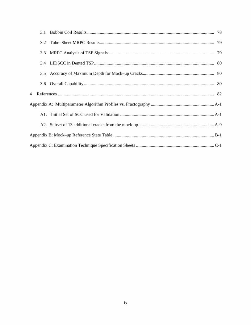
3.1 Bobbin Coil Results ................................................................................................................ 78

3.2 Tube–Sheet MRPC Results..................................................................................................... 79

3.3 MRPC Analysis of TSP Signals.............................................................................................. 79

3.4 LIDSCC in Dented TSP.......................................................................................................... 80

3.5 Accuracy of Maximum Depth for Mock–up Cracks............................................................... 80

3.6 Overall Capability ................................................................................................................... 80

4 References .......................................................................................................................................... 82

Appendix A: Multiparameter Algorithm Profiles vs. Fractography ........................................................ A-1

A1. Initial Set of SCC used for Validation ................................................................................... A-1

A2. Subset of 13 additional cracks from the mock-up................................................................... A-9

Appendix B: Mock–up Reference State Table ......................................................................................... B-1

Appendix C: Examination Technique Specification Sheets ..................................................................... C-1

Figures

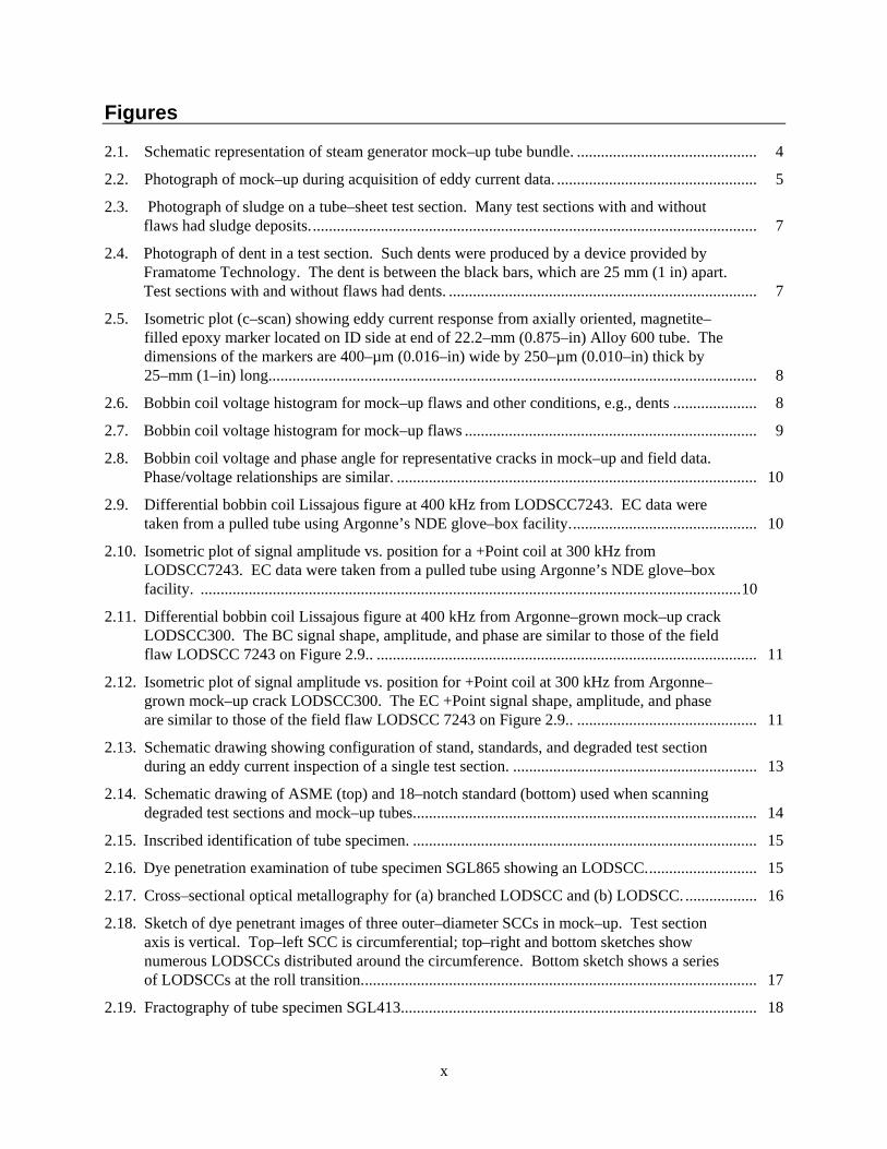
2.1. Schematic representation of steam generator mock–up tube bundle. ............................................. 4

2.2. Photograph of mock–up during acquisition of eddy current data. .................................................. 5

2.3. Photograph of sludge on a tube–sheet test section. Many test sections with and without flaws had sludge deposits................................................................................................................ 7

2.4. Photograph of dent in a test section. Such dents were produced by a device provided by Framatome Technology. The dent is between the black bars, which are 25 mm (1 in) apart. Test sections with and without flaws had dents. ............................................................................. 7

2.5. Isometric plot (c–scan) showing eddy current response from axially oriented, magnetite–filled epoxy marker located on ID side at end of 22.2–mm (0.875–in) Alloy 600 tube. The dimensions of the markers are 400–µm (0.016–in) wide by 250–µm (0.010–in) thick by 25–mm (1–in) long.......................................................................................................................... 8

2.6. Bobbin coil voltage histogram for mock–up flaws and other conditions, e.g., dents ..................... 8

2.7. Bobbin coil voltage histogram for mock–up flaws ......................................................................... 9

2.8. Bobbin coil voltage and phase angle for representative cracks in mock–up and field data. Phase/voltage relationships are similar. .......................................................................................... 10

2.9. Differential bobbin coil Lissajous figure at 400 kHz from LODSCC7243. EC data were taken from a pulled tube using Argonne’s NDE glove–box facility............................................... 10

2.10. Isometric plot of signal amplitude vs. position for a +Point coil at 300 kHz from LODSCC7243. EC data were taken from a pulled tube using Argonne’s NDE glove–box facility. .......................................................................................................................................10

2.11. Differential bobbin coil Lissajous figure at 400 kHz from Argonne–grown mock–up crack LODSCC300. The BC signal shape, amplitude, and phase are similar to those of the field flaw LODSCC 7243 on Figure 2.9.. ............................................................................................... 11

2.12. Isometric plot of signal amplitude vs. position for +Point coil at 300 kHz from Argonne–grown mock–up crack LODSCC300. The EC +Point signal shape, amplitude, and phase are similar to those of the field flaw LODSCC 7243 on Figure 2.9.. ............................................. 11

2.13. Schematic drawing showing configuration of stand, standards, and degraded test section during an eddy current inspection of a single test section. ............................................................. 13

2.14. Schematic drawing of ASME (top) and 18–notch standard (bottom) used when scanning degraded test sections and mock–up tubes...................................................................................... 14

2.15. Inscribed identification of tube specimen. ...................................................................................... 15

2.16. Dye penetration examination of tube specimen SGL865 showing an LODSCC............................ 15

2.17. Cross–sectional optical metallography for (a) branched LODSCC and (b) LODSCC. .................. 16

2.18. Sketch of dye penetrant images of three outer–diameter SCCs in mock–up. Test section axis is vertical. Top–left SCC is circumferential; top–right and bottom sketches show numerous LODSCCs distributed around the circumference. Bottom sketch shows a series of LODSCCs at the roll transition................................................................................................... 17

2.19. Fractography of tube specimen SGL413......................................................................................... 18

x

2.20. Sizes and shapes of LODSCCs in tube specimen AGL 536 determined by EC NDE using the multiparameter algorithm (dotted curve) and fractography (smooth curve). ............................ 19

2.21. Comparison of maximum depths determined by the multiparameter algorithm with that determined by fractography (a) set of 23 cracks; (b) set of 36 cracks; (c) comparison of the best fits to the two sets. ................................................................................................................... 20

2.22. Comparison of depths (% TW) determined by the multiparameter algorithm with those by fractography and regression fit and estimated 95% bounds for the observed depth as a function of the multiparameter depth estimate. Multiple observations from a single crack. .......... 21

2.23. Comparison of maximum depths (% TW) determined by the phase analysis of +Point data with those by fractography. A regression fit and estimated 95% bounds for the observed depth as a function of the +Point depth estimate are also shown.................................................... 21

2.24. Comparison of maximum depth determined by the multiparameter algorithm with metallographic results for the ten specimens that were destructively analyzed. Destructive evaluation (DE) was carried out using metallographic sectioning techniques................................ 22

2.25. Estimates of maximum crack depths by the multiparameter algorithm compared with estimates using +Point phase analysis at 300 kHz. ......................................................................... 22

2.26. Maximum bobbin coil voltage as a function of maximum crack depth for FS and TSP SCC in the mock-up. The eddy current multiparameter algorithm was used to profile the crack and determine the maximum depth. ................................................................................................ 22

2.27. Bobbin coil phase–angle as a function of maximum crack depth for LODSCC at TSPs in the mock-up. The eddy current multiparameter algorithm was used to profile the crack and determine the maximum depth. ....................................................................................................... 23

2.28. Bobbin coil phase–angle as a function of maximum crack depth for mock–up TSP LIDSCC. The eddy current multiparameter algorithm was used to profile the crack and determine the maximum depth. ....................................................................................................... 23

2.29. Standard deviation in percent throughwall as a function of predicted maximum depth. ................ 25

2.30. (a) Crack depth profile measured by eddy current and (b) a candidate equivalent rectangular crack corresponding to depth do = 50% and Lo = 10 mm (0.39 in). ........................... 27

2.31. Ligament rupture pressures corresponding to three candidate equivalent rectangular cracks, 11 mm (0.43 in) by 60%, 9 mm (0.35 in) by 70%, and 7 mm (0.28 in) by 75%. The equivalent rectangular crack is 9 mm (0.35 in) by 70% because these values correspond to the lowest ligament rupture pressure (30 MPa or 4.35 ksi)............................................................. 27

2.32. Photograph of underside of tube bundle. Conduit carrying the EC probe is shown being positioned under a tube. .................................................................................................................. 36

2.33. Isometric plot of mock–up roll transition collected with a rotating +Point coil at 300 kHz (example 1). .................................................................................................................................... 40



2.36. Isometric plot of roll transition from a retired steam generator. ..................................................... 41

xi

2.37. MRPC data plotted for LODSCC at TS with sludge. ..................................................................... 43

2.38. BC data plotted for LODSCC at TSP. ............................................................................................ 43

2.39. MRPC data plotted for LODSCC at TSP........................................................................................ 44

2.40. BC data plotted for LIDSCC in dent at TSP. .................................................................................. 44

2.41. Isometric plot for LIDSCC in dent at TSP...................................................................................... 45

2.42. Isometric plot for CIDSCC at TS with sludge. ............................................................................... 45

2.43. RPC data plotted for IGA at TSP.................................................................................................... 46

2.44 Range of POD curves represented by linear–logistic functions with varying values of the parameters a and b........................................................................................................................... 50

2.45 Linear–logistic, log–logistic, and linear–log–log fits to mockup inspection data for longitudinal OD SCC at tube support plates. .................................................................................. 56

2.46. Effect of the choice of depth (identified as % TW) at which to impose the false call constraint on log–logistic fits for the POD curve for LODSCC at the TSP. The choice of the 5% TW depth gives the optimum fit. ........................................................................................ 57

2.47. Cumulative distribution of normalized standard deviations for bobbin coil voltages for LODSCC at tube support plates. ..................................................................................................... 58

2.48. BC POD for TSP data as a function of maximum depth for LODSCC and LIDSCC using maximum likelihood fits; (a) linear–logistic fit and the one–sided 95% confidence limit (OSL) including uncertainty in the maximum depth; (b) linear–logistic, linear log–log, and log–logistic fits for LODSCC. The solid curve in each figure is the best–fit to the data. ............. 59

2.49. BC POD for TSP data as a function of maximum depth (as fraction through–wall) for LODSCC using maximum likelihood fits. The fits are to data from one team only. The circles show the raw data from which the curve is generated. Depths are determined with the multiparameter algorithm. Although the log–logistic is the best–fit, differences between the models for this team are not statistically significant. .................................................. 59

2.50. BC POD for free–span data as a function of maximum depth (as fraction throughwall) for LODSCC by using maximum likelihood fits to linear–logistic, linear log–log, and log–logistic curves. Depths are determined with the multiparameter algorithm................................... 60

2.51. BC POD for LIDSCC at the TSP data as a function of maximum depth (as fraction throughwall) by using maximum likelihood linear logistic fit........................................................ 60

2.52. Round–robin resolution analysts’ results as a function of BC voltage for TSP crack. The BC POD has been evaluated for LODSCC at the TSP. .................................................................. 60

2.53. Log–logistic fits for BC POD as a function of voltage for LODSCC in TSP. POPCD is a voltage–based POD curve developed by industry........................................................................... 61

2.54. BC POD by team for free–span and TSP LODSCC combined as a function of depth. The maximum crack depth (as fraction of wall) was determined by the multiparameter algorithm. The highest solid line represents the best team, the lowest dashed line represents the worst team, and the other symbols represent the remaining teams. .......................................... 62

2.55. BC POD by team for free–span LODSCC as function of depth. The maximum crack depth (as fraction of wall) was determined by the multiparameter algorithm. The solid line represents the best team, while the symbols and dashed line represent the remaining teams. ........ 62

xii

2.56. BC POD for TSP LODSCC as a function of mp. Curves derived by maximum likelihood fit and an estimate of the one–sided 95% confidence limit. The values of mp are derived by using depths from the multiparameter algorithm. ........................................................................... 63

2.57. BC POD for free–span data for LODSCC as a function of mp. Curves derived by maximum likelihood fit and an estimate of the one–sided 95% confidence limit. The values of mp are derived by using depths from the multiparameter algorithm. ......................................................... 63

2.58. Tube–sheet MRPC POD as a function of maximum depth (as fraction of wall) for axial and circumferential inner–diameter SCC. Depths are determined with the multiparameter algorithm. ........................................................................................................................................ 65

2.59. Tube–sheet MRPC POD by team as a function of maximum depth (as fraction of wall) for axial and circumferential IDSCC and ODSCC. Maximum depth is estimated by the multiparameter algorithm. The solid line represents the best team, the dashed line represents the worst team, and the symbols represent the remaining teams. .................................. 66

2.60. Tube–sheet MRPC POD as a function of maximum depth (as fraction of wall) for LODSCC and CODSCC combined. All three statistical models have similar goodness of fit measures so that model uncertainty is large over a significant fraction of the depth. Depths are determined with the multiparameter algorithm. .............................................................................. 66

2.61. Tube–sheet MRPC POD for ID axial and circumferential SCC combined as a function of maximum depth (as fraction of wall). Depths estimated by conventional phase analysis with a +Point™ probe (pp) and by the multiparameter method (mp). ............................................ 66

2.62. Tube–sheet BC and MRPC POD for CIDSCC and LIDSCC. Depths are determined with the multiparameter algorithm. ......................................................................................................... 67

2.63. Tube–sheet BC and MRPC POD for LIDSCC. Depths are determined with the multiparameter algorithm................................................................................................................ 67

2.64. Depth profiles of TSP LODSCC with maximum depth of 99% TW that was missed by all teams analyzing MRPC data. The largest piece of the segmented crack has a length of about 10 mm (0.4 in). The lower part of the figure shows the crack along the test section axis. ........................................................................................................................................... 68

2.65. Bobbin coil voltage as a function of maximum depth of LIDSCC in a TSP dent. These data show no correlation between BC voltage and LIDSCC depth. The depth was determined by application of Argonne’s multiparameter algorithm to MRPC data. ......................................... 70

2.66. Number of teams out of 11 correctly calling LIDSCC in a dented TSP from mock–up bobbin coil data (using resolution analyst reports) as a function of maximum crack depth. The depth was determined by application of Argonne’s multiparameter algorithm to MRPC data. ........................................................................................................................................... 70

2.67. Number of teams out of 11 correctly calling LIDSCC in a dented TSP from mock–up bobbin coil data (using resolution analyst reports) as a function of BC voltage............................. 70

2.68. Number of teams out of 10 correctly calling an LIDSCC in a dented TSP from mock–up bobbin coil data followed by a correct call for that crack using MRPC data (from resolution analyst reports) as a function of maximum crack depth. The depth was determined by application of Argonne’s multiparameter algorithm to MRPC data. .............................................. 71

2.69. Number of teams out of 10 correctly calling an LIDSCC in a dented TSP from bobbin coil data followed by dismissing that crack using MRPC data (from resolution analyst reports)

xiii

as a function of maximum crack depth. The depth was determined by application of Argonne’s multiparameter algorithm to MRPC data. ..................................................................... 71

2.70. Number of teams out of 10 missing an LIDSCC in a dented TSP from bobbin coil data followed by a correct call using MRPC data (from resolution analyst reports) as a function of maximum crack depth. The depth was determined by application of Argonne’s multiparameter algorithm to MRPC data. ....................................................................................... 71

2.71. Number of teams out of 10 missing an LIDSCC in a dented TSP with both bobbin coil and MRPC data (from resolution analyst reports) as a function of maximum crack depth. The depth was determined by application of the multiparameter algorithm to MRPC data. ................. 72

2.72. Number of false calls in dented TSP test sections as a function of BC voltage (0.1–V window). ......................................................................................................................................... 72

2.73. Number of teams correctly calling an LIDSCC in a dented TSP using MRPC data (from resolution analyst reports) as a function of maximum crack depth. The depth was determined by application of Argonne’s multiparameter algorithm to MRPC data. ...................... 72

2.74. Number of teams out of 11 correctly calling IGA from bobbin coil data (using resolution analyst reports) as a function of maximum flaw depth. The depth was determined by application of Argonne’s multiparameter algorithm to MRPC data. .............................................. 73

2.75. Number of teams out of 11 correctly calling EDM and laser cut slots (LAS) from bobbin coil data (using resolution analyst reports) as a function of maximum depth. The location and type of notch missed is indicated in the graph. ........................................................................ 74

2.76. POD for Tube–sheet MRPC as a function of maximum depth (as fraction of wall) for axial and circumferential IDSCC and ODSCC grown at Argonne and cracks grown using doped steam technique. Depths are determined with the multiparameter algorithm. ............................... 74

2.77. POD with 95% one–sided confidence limits for TSP LODSCC with magnetite on the tube OD surface. ..................................................................................................................................... 75

2.78 POD using MRPC data for OD and ID SCC at the RTZ with sludge above the tube-sheet........... 76

2.79. Fractional detection rate for wastage and wear using bobbin coil data. ......................................... 76

A1. AGL 2241 CODSCC: EC NDE depth versus position using the multiparameter algorithm (dotted curve) and fractography depth versus position (smooth curve). ......................................... A-1

A2. AGL 2242 CIDSCC: EC NDE depth versus position using the multiparameter algorithm (dotted curve) and fractography depth versus position (smooth curve). ......................................... A-1

A3. AGL 288 LIDSCC: EC NDE depth versus position using the multiparameter algorithm (dotted curve) and fractography depth versus position (smooth curve). ......................................... A-2


A5. AGL 533 LODSCC: EC NDE depth versus position using the multiparameter algorithm (dotted curve) and fractography depth versus position (smooth curve). ......................................... A-2



xiv

















A24. Test section 42 removed from mock–up with a CODSCC. EC NDE depth versus position using the multiparameter algorithm (dotted curve) and fractography depth versus position (smooth curve). ............................................................................................................................... A-9

A25. Test section 43 removed from mock–up with a CODSCC. EC NDE depth versus position using the multiparameter algorithm (dotted curve) and fractography depth versus position (smooth curve). ............................................................................................................................... A-9

A26. Test section 45 removed from mock–up with a CODSCC. EC NDE depth versus position using the multiparameter algorithm (dotted curve) and fractography depth versus position (smooth curve). ...............................................................................................................................A-10

xv

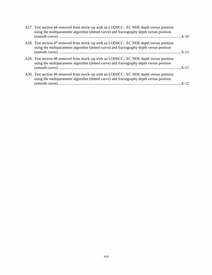
A27. Test section 44 removed from mock–up with an LODSCC. EC NDE depth versus position using the multiparameter algorithm (dotted curve) and fractography depth versus position (smooth curve). ...............................................................................................................................A-10




xvi

Tables

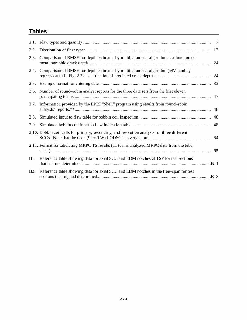
2.1. Flaw types and quantity................................................................................................................... 7

2.2. Distribution of flaw types. ............................................................................................................... 17

2.3. Comparison of RMSE for depth estimates by multiparameter algorithm as a function of metallographic crack depth.............................................................................................................. 24

2.4. Comparison of RMSE for depth estimates by multiparameter algorithm (MV) and by regression fit in Fig. 2.22 as a function of predicted crack depth.................................................... 24

2.5. Example format for entering data .................................................................................................... 33

2.6. Number of round–robin analyst reports for the three data sets from the first eleven participating teams........................................................................................................................... 47

2.7. Information provided by the EPRI “Shell” program using results from round–robin analysts’ reports.**.......................................................................................................................... 48

2.8. Simulated input to flaw table for bobbin coil inspection................................................................. 48

2.9. Simulated bobbin coil input to flaw indication table....................................................................... 48

2.10. Bobbin coil calls for primary, secondary, and resolution analysts for three different SCCs. Note that the deep (99% TW) LODSCC is very short. ....................................................... 64

2.11. Format for tabulating MRPC TS results (11 teams analyzed MRPC data from the tube-sheet). .............................................................................................................................................. 65

B1. Reference table showing data for axial SCC and EDM notches at TSP for test sections that had mp determined. ..................................................................................................................B–1

B2. Reference table showing data for axial SCC and EDM notches in the free–span for test sections that mp had determined......................................................................................................B–3

xvii


xviii

Executive Summary

A major outcome of regulatory activity over the past 10 years has been the development and implementation of two key concepts, condition monitoring and operational assessment. That effort was intended to develop guidance for tube integrity assessments. Condition monitoring is an assessment of the current state of the steam generator (SG) relative to the performance criteria for structural integrity and leakage. An operational assessment involves an attempt to assess the state of the generator relative to the structural integrity and leakage performance criteria at the end of the next inspection cycle. Predictions of the operational assessment from the previous cycle can be compared with the condition monitoring assessment to verify the adequacy of the methods and data used to perform the operational assessment.

The reliability of the in-service inspection is critical to the effectiveness of the operational assessment and condition monitoring is the reliability of the nondestructive evaluation (NDE) techniques used to establish the flaw distribution. An NDE round–robin exercise has been used to independently assess SG inspection reliability. This exercise employed a steam generator mock–up at ANL. The purpose was to assess the current state of in–service inspection (ISI) reliability for SG tubing, determine the probability of detection (POD) as a function of flaw size or severity, and assess the capability for flaw sizing. Note that this report does not establish a regulatory position.

Eleven teams participated in analyzing bobbin and rotating probe data from the mock–up that were collected by qualified industry personnel. The mock–up tube bundle contains hundreds of cracks and simulations of artifacts such as corrosion deposits, support structures, and tube geometry variations that, in general, make the detection and characterization of cracks more difficult. An expert NDE Task Group from ISI vendors, utilities, EPRI, ANL, and the NRC has reviewed the eddy current signals from laboratory–grown cracks used in the mock–up to ensure that they provide a realistic simulation of those obtained in the field. The number of tubes inspected and the number of teams participating in the round–robin are expected to provide better statistical data on the POD and characterization accuracy than is currently available from industry performance–demonstration programs.

The mock–up tube bundle consists of 400 Alloy 600 tubes, each divided into nine test sections, 0.3 m (1 ft) long. The test sections are arranged in nine levels. The lowest level simulates the tube-sheet, while three other levels simulate tube support plate (TSP) intersections. The remaining five levels are free–span (FS) regions. Tubes rolled into ferritic steel collars simulate the tube-sheet geometry. Thus, both the roll transition geometry and the effect of the ferritic tube-sheet are simulated. Axial and circumferential cracks are present in the roll transition region. In the TSP crevice, the presence of magnetite was simulated by filling the crevice with magnetic tape or a ferromagnetic fluid. A mixture of magnetite and copper powder in an epoxy binder simulated sludge deposits. Longitudinal outer–diameter stress corrosion cracks (LODSCC), both planar and segmented, and cracks in dents with varying morphologies are present at TSP locations. Cracks in the five FS levels are primarily LODSCC, both planar and segmented. Other types of flaws such as intergranular attack (IGA) and wear are found in the tube bundle but in small numbers.

Bobbin coil (BC) data were collected on all 3600 test sections of the mock–up by using magnetically biased (“mag–biased”) probes. A mag–biased, rotating, three–coil probe was used to collect data from all 400 tube-sheet and special–interest test sections. This motorized rotating pancake coil (MRPC) probe included a midrange +Point coil, a 2.9–mm (0.115–in)–diameter pancake coil, and a 2–mm (0.080–in)–diameter, high–frequency, shielded pancake coil. Eddy current data were collected by a qualified industry team and stored on optical disks. Round–robin (RR) teams later analyzed the data with an ANL proctor present to monitor the analysis process. The intent was to make the analysis as close a

xix

simulation of an actual inspection as possible. The procedures and training sets were developed in cooperation with the NDE Task Group so that the inspection protocols and training would mimic those in current practice.

The reference state for each flaw in the mock–up, i.e., crack geometry and size, was established by calculations using a multiparameter algorithm developed at ANL for analyzing eddy current (EC) data. Both pre– and post–assembly inspection results were used for this purpose. Throughout the development stage of the algorithm, comparisons were made between the NDE predictions and results obtained by destructive analyses for dozens of flaws. A blind test was performed comparing the NDE results to destructive analyses on a set of 23 flawed specimens. The results from this comparison were used to make an initial estimate of the uncertainties associated with the depth estimates from the multiparameter algorithm. Further validation was carried out by destructive examination of 13 additional tubes removed from the mock–up. Inclusion of this additional data had a small effect on the initial estimates of the uncertainties in the depth measurements and their effects on the POD curves.

Eleven teams participated in the analysis round–robin. Each team provided nine reports: a primary analyst report, a secondary analyst report, and a resolution analyst report for each of the three optical data disks containing the inspection results (bobbin coil for all tubes, MRPC for all tube–sheet test sections, and MRPC for a set of selected test sections). Results were analyzed for all teams, including the team–to–team variation in the POD, along with the population average. Analysis of the LODSCC data at the tube support plate and in the free–span showed that BC false call rates are about 2% for the TSP and 0.1% for the free–span. The BC false call rate for longitudinal inner–diameter stress corrosion cracks (LIDSCC) in dents is very high (44%); the final resolution is based on MRPC results. The MRPC false call rate for flaws at the top of the tube-sheet is about 6%.

The BC POD for TSP inner-diameter SCC is higher than for outer–diameter SCC, although this conclusion should be tempered in light of the large difference in false call rates. The BC POD for free–span LODSCC is higher than the POD for TSP LODSCC, but lower than that for TSP LIDSCC. However, the comparison with LIDSCC should also consider the difference in false call rates. For the MRPC in the tube-sheet, the POD for inner-diameter SCC is about 75% with an one–sided 95% confidence limit of about 65%. The highest tube-sheet MRPC POD curve is for LIDSCC, where the POD for 60% through wall flaws is 85%.

A review was carried out of MRPC results for BC voltages from 2.0 to 5.6 V. Such calls are normally made to confirm or dismiss the BC flaw call. The result for LODSCC > 75% TW, which are of greatest concern in terms of integrity, is an average correct call of 98%. However, even with MRPC data all teams missed an LODSCC at the TSP with an estimated maximum depth of 39% TW. Another test section had a flaw with an estimated maximum depth of 99% TW, but signal from the +Point coil at 300 kHz was only a few tenths of a volt. This sample shows that it is possible to have a strong BC signal and a weak MRPC signal that would not be called a crack.

The detection results for the 11 teams were used to develop POD curves as a function of maximum depth and the parameter mp, a stress multiplier that relates the stress in the ligament ahead of the crack to the stress in an unflawed tube under the same loading. Because mp incorporates the effect of both crack depth and length, it better characterizes the effect of a flaw on the structural and leakage integrity of a tube than do traditional indicators, such as maximum depth. When the PODs are considered as a function of mp in the TSP and FS regions, the POD for cracks that would fail or leak under 3p internal pressure (corresponding to mp ≈ 2.3) is > 95%, even when uncertainties are accounted for.

xx

The POD curves were represented as linear–logistic curves, log–logistic, or linear–log–log fits and the curve parameters were determined by the method of maximum likelihood. The statistical uncertainties inherent in sampling from distributions and the uncertainties due to errors in the estimates of maximum depth and mp were determined. The 95% one–sided confidence limits (OSLs), which include errors in maximum depth estimates, are presented along with the POD curves.

For the mockup inspection data, the linear–logistic, log–logistic, and linear–log–log fits are in some cases statistically indistinguishable. This is because the bulk of the mockup cracks are deep and for deep cracks the different statistical fits give similar results. For very shallow cracks, the results are fixed by the false–call rate. For depths in the intermediate region, where the different fits have different types of behavior. there may be few cracks, and the measures of differences in fit may not be statistically significant. These features make it difficult to determine a “best fit”.

POD curves are also sensitive to variability in signal–to–noise ratio. Because the results are based on test sections with a variety of local noise levels, the curves developed in this report represent POD curves representative of the average local noise level in the ANL Steam Generator Mockup. The average local noise level in operating steam generators is probably somewhat higher than in the mockup, although this must be addressed case–by–case. The variability in local noise levels within a given facility such as the mockup is also important. The POD curves represent the probability that a flaw of a given depth or with a given voltage signal will be detected at the average local noise level. For locations with higher or lower local noise levels, the POD for a flaw of a given depth will be smaller or greater than the POD for the average level.

The results were analyzed by team to determine whether there was a strong team–to–team variation in the POD. The performances of most of the teams cluster rather tightly, although in some cases a significant variation existed between the best and the worst. The probability that the team–to–team variations in the logistic fits to the data were due to chance was estimated. For LIDSCC at the TSP, the variation from best to worst is very significant statistically. The probability is < 0.1% that the difference is due to chance. For free span (FS) ODSCC, the variation from best to worst is likely to be significant, i.e., the likelihood that it is due to chance is < 20%. For TSP ODSCC, this variability is probably not significant, i.e., the likelihood that it is due to chance is > 60%.

The BC voltages reported for LODSCC indications at TSP regions were also analyzed. In most cases, the differences in the voltage reported by the different teams were small. This finding, in part, is attributed to the fact that all teams analyzed the same set of data, i.e., had identical data acquisition and calibration setups. For each longitudinal ODSCC indication, an average BC voltage and a corresponding standard deviation were computed for all teams. For almost 85% of all indications, the normalized standard deviation in the reported voltage is < 0.1 V. Indications with larger variations are not associated with particularly high or low voltage values (i.e., approximately half the signals with standard deviations of > 0.1 V have voltages of > 2 V). Instead, they are associated with the complexity of the signal and the difficulty of identifying the peak voltage and the associated null position.

The round–robin results for the small number of test sections with IGA have been analyzed separately from the other flawed test sections. The result suggests that this type of volumetric cracking can be detected easily with a bobbin coil for depths greater than 40% TW.

The BC results for electro–discharged machined (EDM) notches and laser–cut slots have also been analyzed as a subset of the mock–up. For depths 40% TW and greater, the success in detecting notches and laser–cut slots is greater than for SCCs of comparable depths. This finding suggests that POD curves generated using notches are unrealistically high for deep cracks.

xxi

Acknowledgments

The authors thank C. Vulyak and L. Knoblich for their contributions to the experimental effort, and P. Heasler and R. Kurtz for discussions related to the statistical analysis. The authors thank NDE Task Group Members G. Henry and J. Benson (EPRI), T. Richards and R. Miranda (Framatome Technology), D. Adamonis and R. Maurer (Westinghouse), D. Mayes (Duke Engineering and Services), S. Redner (Northern States Power), and B. Vollmer and N. Farenbaugh (Zetec). Thanks also to H. Houserman and H. Smith for their input in this effort. The authors acknowledge the contributions of C. Gortemiller, C. Smith, S. Taylor, and the staff from Zetec, Inc. to the data acquisition and analysis effort. The authors also thank proctors S. Gopalsami, K. Uherka, and M. Petri, as well as ASEA Brown–Boveri–Combustion Engineering, Anatec, Duke Engineering and Services, Framatome Technology, KAITEC, Ontario Power Generation, Westinghouse, and Zetec, for providing round–robin analysis teams. This work is sponsored by the Office of Nuclear Regulatory Research, U.S. Nuclear Regulatory Commission, under Job Code W6487, Dr. J. Muscara provided very helpful guidance in the performance of this work.

xxii

Acronyms and Abbreviations

ABB–CE ASEA Brown–Boveri–Combustion Engineering AECL Atomic Energy of Canada, Ltd. ANL Argonne National Laboratory ASME American Society of Mechanical Engineers BC bobbin coil CIDSCC circumferential inner–diameter stress corrosion crack/cracking CODSCC circumferential outer–diameter stress corrosion crack/cracking DE&S Duke Engineering and Services DTC difference due to chance EC eddy current ECT eddy current testing EDM electro–discharge machining EPRI Electric Power Research Institute ETSS examination technique specification sheet FS free–span FTI Framatome Technology–ANP ID inner diameter IDSCC inner–diameter stress corrosion crack/cracking IGA intergranular attack INEEL Idaho National Engineering and Environmental Laboratory ISI in–service inspection LIDSCC longitudinal inner–diameter stress corrosion crack/cracking LODSCC longitudinal outer–diameter stress corrosion crack/cracking MLE maximum likelihood estimate MRPC motorized rotating pancake coil NDD nondetectable degradation NDE nondestructive evaluation NRC U.S. Nuclear Regulatory Commission OD outer diameter ODSCC outer–diameter stress corrosion crack/cracking OPG Ontario Power Generation OSL one–sided 95% confidence limit PNNL Pacific Northwest National Laboratory POD probability of detection PWR pressurized water reactor PWSCC primary–water stress corrosion crack/cracking QDA qualified data analyst RMSE root mean square error RPC rotating pancake coil RR round–robin RTZ roll transition zone SCC stress corrosion crack/cracking SG steam generator SSPD site–specific performance demonstration TS tube-sheet TSP tube support plate TTS top of tube-sheet TW throughwall UT ultrasonic testing W Westinghouse

xxiii


xxiv

1 Introduction

A major outcome of the regulatory activity to develop guidance for tube integrity assessments over the past 10 years was the development and implementation of two key concepts, condition monitoring and operational assessment. Condition monitoring is an assessment of the current state of the steam generator (SG) relative to the performance criteria for structural and leakage integrity. An operational assessment is an attempt to assess the state of the SG relative to the structural and leakage integrity performance criteria at the end of the next inspection cycle. The predictions of the operational assessment from the previous cycle can be compared with the results of the condition monitoring assessment to verify the adequacy of the methods and data used to perform the operational assessment. The reliability of the in–service inspection (ISI) is critical to the effectiveness of the assessment processes. Quantitative information on probability of detection (POD) and sizing accuracy of flaws of inspection techniques used for SG tubes is needed to determine if tube integrity performance criteria were met during the last operating cycle, and if performance criteria for SG tube integrity will continue to be met until the next scheduled ISI. An increased understanding of inspection reliability permits better estimation of the true state of SG tubes after an ISI. Similarly, knowledge of sizing accuracy allows corrections to be made to flaw sizes obtained from ISI.

Eddy–current (EC) inspection techniques are the primary means of ISI for assessing the condition of SG tubes. Detection of flaws by EC techniques depends on detecting the changes in impedance produced by a flaw. Although the relative impedance changes are small (≈1/106), they are readily detected by modern electronic instrumentation. However, many other factors, including tube material properties, tube geometry, and degradation morphology, can produce impedance changes, and the capability to distinguish between the changes produced by such artifacts and those produced by flaws is strongly influenced by EC data acquisition practices (including human factors) and data analysis procedures. Similarly, although there is a physics–based relationship between the depth of a defect into the tube wall and the EC signal phase response, the factors discussed above that affect detection also affect sizing capability.

The most desirable approaches to establish the reliability of current ISI methods would be to carry out round–robin (RR) exercises where a number of teams would perform inspections on either operating SGs or those removed from service. However, access to such facilities for this purpose is difficult, and validation of the results would be difficult. Such work would also very expensive. In addition, obtaining data on all morphologies of interest could require tubes from or access to many different plants.

The approach chosen for this program was to develop an SG tube bundle mock–up that simulates the key features of an operating SG so that the inspection results from the mock–up would be expected to be representative of those for operating SGs. The mock–up is also being used as a test bed for evaluating emerging technologies for the ISI of SG tubes. Considerable effort was expended in preparing realistic flaws and verifying that their EC signals and morphologies are representative of those from operating SGs. The mock–up includes stress corrosion cracks of different orientations and morphologies at various locations in the mock–up and simulates the artifacts and support structures that can affect the EC signals. Factors that influence detection of flaws include probe wear, EC signal noise, signal–to–noise ratio, analyst fatigue, and the subjective nature of interpreting complex EC signals. None of these factors were explicitly addressed in the study, but they were implicitly included and affected the results. In this exercise, all analysts analyzed the same data, which were provided on optical disks. The team–to–team variation in detection capability is the result of analyst variability in interpretation of EC signals. The fits to the POD data and the subsequent lower 95% confidence limits are influenced by the uncertainty in crack depths determined by a multiparameter algorithm and the number of cracks in the sample set.

1

This report includes revised POD curves based on additional destructive examination of specimens from the mockup and reconsideration of the uncertainties associated with the choice of statistical models to fit the data. In this report, although the probabilities of detecting flaws of various types and at various locations are presented, the results do not establish regulatory position.

2

2 Program Description

The overall objective of the SG tube integrity program [2] is to provide the experimental data and predictive correlations and models needed to permit the NRC to independently evaluate the integrity of SG tubes as plants age and degradation proceeds, new forms of degradation appear, and new defect–specific management schemes are implemented. The objective of the inspection task is to evaluate and quantify the reliability of current and emerging inspection technology for current–day flaws, i.e., establish the probability of detection (POD) and sizing accuracy for different size cracks. Both EC and ultrasonic testing (UT) techniques are being evaluated, although only EC testing organizations have participated in the round–robin up to now.

The procedures and processes for the round–robin (RR) studies mimic those currently practiced by commercial teams in actual inspections. Teams participating in the RR exercise report their data analysis results on flaw types, sizes, and locations, as well as other commonly used parameters such as signal amplitude (voltage) and phase.

An important part of the RR exercise was the NDE Task Group, an expert group from ISI vendors, utilities, EPRI, ANL, and the NRC. This group reviewed the signals from the laboratory–grown cracks used in the mock–up to ensure that they provide reasonable simulations of those obtained from real cracks. The Task Group provided input on the quality of the mock–up data, the nature of the flaws, and procedures for data acquisition, analysis, and documentation. To the extent possible, the intent was to mimic current industry practices.

Because the destructive examination of all the flaws in the mock–up would be extremely expensive and time–consuming, several laboratory NDE methods (including various EC and UT procedures) were evaluated as a way to characterize the defects in the mock–up tubes so that the reference state can be estimated without destructive examinations. Based on these evaluations, multiparameter analysis of rotating probe data that was implemented at ANL was used to determine the reference state of the mock–up test sections [3]. This effort has provided sizing estimates for the tube bundle defects. The multiparameter algorithm was initially validated by using 23 test sections with SCCs like those in the mock–up. The depth profiles generated by the multiparameter algorithm were compared to profiles of test sections destructively analyzed with cracks mapped by fractography techniques. These results were further validated by the destructive examination of 13 test sections from the mock–up.

2.1 Steam Generator Mock–up Facility

The mock–up tube bundle consists of 400, 22.2–mm (0.875–in)–diameter, Alloy 600 tubes consisting of 9 test sections, each 0.3 m (1 ft) long. The tube sections are arranged in nine levels with 400 tubes at each elevation. The centers of the tubes are separated by 3.25 cm (1.28 in). Tie rods hold the test sections together. The ends of each test section are pressed into 19–mm (0.75–in)–thick high–density polyethylene plates that hold it in alignment. One end of each tube is spring–loaded. The lowest level (A) has a roll transition zone (RTZ) and simulates the tube-sheet, while the 4th, 7th, and 9th levels simulate intersections of the drilled hole tube support plate (TSP). The other five levels are free–span regions. Above the 9th level is a 0.91–m (3–ft)–long probe run–out section. See Fig. 2.1 for the tube bundle diagram, and Fig. 2.2 for a photograph of the mock–up. Debris generated during assembly (e.g., shavings from the polyethylene plates) was cleared to assure that the eddy current probes could travel unobstructed through all test sections.

3

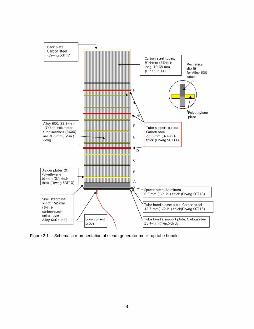
Figure 2.1. Schematic representation of steam generator mock–up tube bundle.

4

Figure 2.2. Photograph of mock–up during acquisition of eddy current data.

5

Most of the degraded test sections were produced at ANL, although some were produced by Pacific Northwest National Laboratory (PNNL); Westinghouse; Equipos Nucleares, SA (ENSA); and the Program for the Inspection of Steel Components (PISC).

The test sections in the tube-sheet level are all mechanically expanded into a 30.5–cm (6–in)–long carbon steel collar, leaving a RTZ halfway from the tube end. To produce cracks in and near the RTZ, the steel collar was split and removed from the expanded tube. Cracking was induced by exposing the expanded test specimen to a chemical solution. Axial and circumferential outer diameter (OD) and inner diameter (ID) stress corrosion cracks (SCC) were produced in the RTZs. New steel collars that were expanded by heating were slipped over the cracked tubes. This process produced flawed test sections with realistic EC signals.

In the TSP regions, filling the crevice with magnetic tape or a ferromagnetic fluid simulated magnetite in the crevices. A mixture of magnetite and copper bonded with epoxy simulated sludge deposits. Sludge was placed above the RTZ and at TSP intersections in some cases (see Fig. 2.3 for photograph of sludge on a tube-sheet test section). Many test sections had sludge or magnetite but no flaws. LODSCC and LIDSCC, both planar and segmented, and cracks with varying morphologies are present at TSP locations with and without denting (see Fig. 2.4 for a photograph of a dent). Some flaw–free test sections were dented. Cracks in the remaining five free–span levels are primarily LODSCC, both planar and segmented. Axial and circumferential cracks of ID and OD origin are found in the RTZ. A small number of other flaw types such as IGA and wear are placed in the tube bundle. The mock–up also contains test sections with electro–discharge–machined (EDM) notches and laser–cut slots. Table 2.1 summarizes the degradation types and their locations in the mock–up. Flaw types included IGA, outer–diameter SCC, primary–water or ID SCC (PWSCC), wear/wastage, and fatigue.

Magnetite–filled epoxy markers were placed at the ends of all test sections to provide a reference for the angular location of flaws when collecting data with a rotating or array probe. Figure 2.5 shows an isometric plot (c–scan) indicating the EC response from an axially oriented, magnetite–filled epoxy marker that is 400–µm (0.016–in) wide by 250–µm (0.010–in) thick by 25–mm (1–in) long and, located on the ID side at the end of a test section. The data were acquired at 400 kHz with a 2.03–mm (0.080–in)–diameter, high–frequency, shielded pancake coil. This test section also contains an outer–diameter SCC at the TSP intersection region. The analysts were instructed to ignore the region 25 mm (1 in) from each test section end when carrying out their analysis.

Prior to assembly, flawed test sections in the tube bundle were examined with both a bobbin coil (BC) and a three–coil rotating probe that incorporates a +Point coil, a 2.9–mm (0.115–in) pancake coil, and a 2–mm (0.080–in) shielded pancake coil. In addition to a full EC examination, many cracked test sections were examined by the dye-penetrant method before being incorporated into the mock–up tube bundle. If EC data or dye-penetrant results indicated that a crack was present, the test section was included in the mock–up. Because primary interest is with deep flaws, the majority of cracks selected for the mock–up had a +Point phase angle consistent with deep (> 60% TW) cracks. Note that since the importance of obtaining POD data from deep flaws is greater than that for shallow ones, high voltage signals are more prevalent in the mock–up than in operating steam generators.

BC data from the mock–up were analyzed to show the distribution of voltages. The histograms (Figs. 2.6 and 2.7) show a reasonable distribution of BC voltages (up to 20 V) for cracks and other conditions, and for cracks alone. Figure 2.6 shows the distribution for all the signals in the mock–up

6

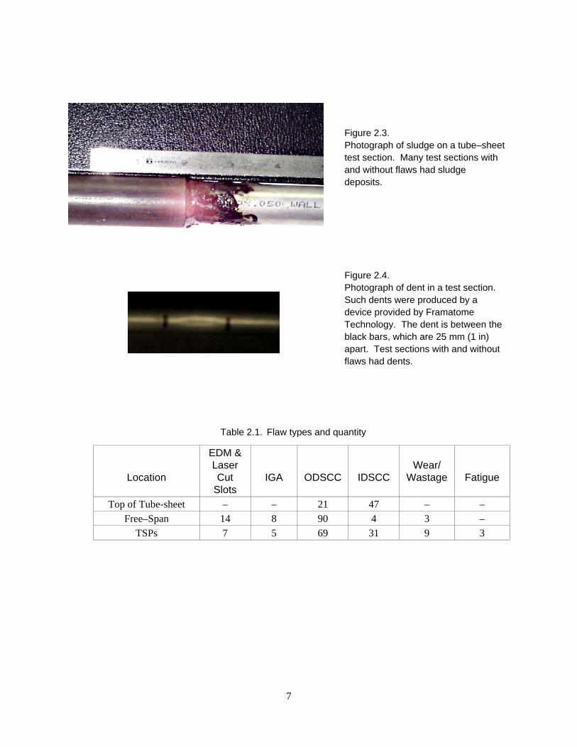
Figure 2.3. Photograph of sludge on a tube–sheet test section. Many test sections with and without flaws had sludge deposits.

Figure 2.4. Photograph of dent in a test section. Such dents were produced by a device provided by Framatome Technology. The dent is between the black bars, which are 25 mm (1 in) apart. Test sections with and without flaws had dents.

Table 2.1. Flaw types and quantity

Location

EDM & Laser Cut

Slots

IGA

ODSCC

IDSCC

Wear/

Wastage

Fatigue

Top of Tube-sheet – – 21 47 – –

Free–Span 14 8 90 4 3 –

TSPs 7 5 69 31 9 3

7

Figure 2.5. Isometric plot (c–scan) showing eddy current response from axially oriented, magnetite–

filled epoxy marker located on ID side at end of 22.2–mm (0.875–in) Alloy 600 tube. The dimensions of the markers are 400–µm (0.016–in) wide by 250–µm (0.010–in) thick by 25–mm (1–in) long.

Figure 2.6. Bobbin coil voltage histogram for mock–up flaws and other conditions, e.g., dents

8

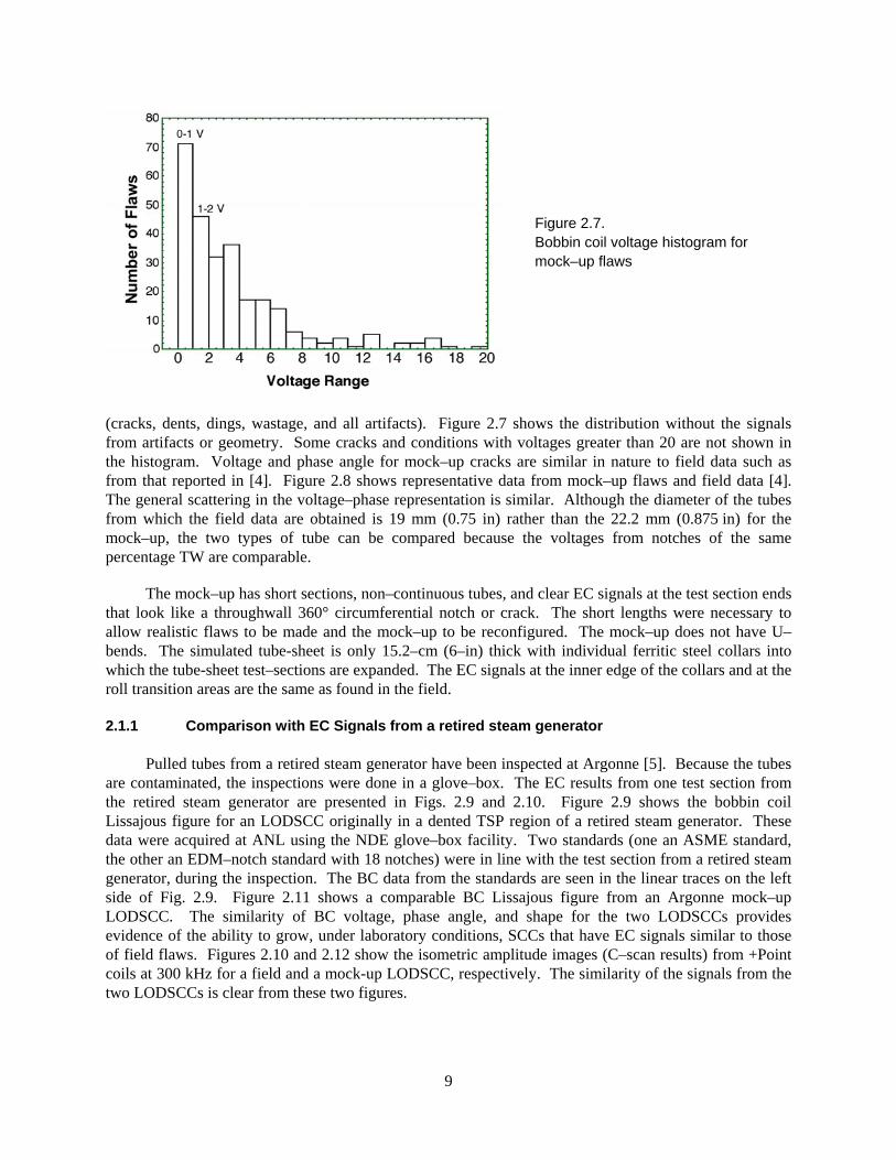
Figure 2.7. Bobbin coil voltage histogram for mock–up flaws

(cracks, dents, dings, wastage, and all artifacts). Figure 2.7 shows the distribution without the signals from artifacts or geometry. Some cracks and conditions with voltages greater than 20 are not shown in the histogram. Voltage and phase angle for mock–up cracks are similar in nature to field data such as from that reported in [4]. Figure 2.8 shows representative data from mock–up flaws and field data [4]. The general scattering in the voltage–phase representation is similar. Although the diameter of the tubes from which the field data are obtained is 19 mm (0.75 in) rather than the 22.2 mm (0.875 in) for the mock–up, the two types of tube can be compared because the voltages from notches of the same percentage TW are comparable.

The mock–up has short sections, non–continuous tubes, and clear EC signals at the test section ends that look like a throughwall 360° circumferential notch or crack. The short lengths were necessary to allow realistic flaws to be made and the mock–up to be reconfigured. The mock–up does not have U–bends. The simulated tube-sheet is only 15.2–cm (6–in) thick with individual ferritic steel collars into which the tube-sheet test–sections are expanded. The EC signals at the inner edge of the collars and at the roll transition areas are the same as found in the field.

2.1.1 Comparison with EC Signals from a retired steam generator

Pulled tubes from a retired steam generator have been inspected at Argonne [5]. Because the tubes are contaminated, the inspections were done in a glove–box. The EC results from one test section from the retired steam generator are presented in Figs. 2.9 and 2.10. Figure 2.9 shows the bobbin coil Lissajous figure for an LODSCC originally in a dented TSP region of a retired steam generator. These data were acquired at ANL using the NDE glove–box facility. Two standards (one an ASME standard, the other an EDM–notch standard with 18 notches) were in line with the test section from a retired steam generator, during the inspection. The BC data from the standards are seen in the linear traces on the left side of Fig. 2.9. Figure 2.11 shows a comparable BC Lissajous figure from an Argonne mock–up LODSCC. The similarity of BC voltage, phase angle, and shape for the two LODSCCs provides evidence of the ability to grow, under laboratory conditions, SCCs that have EC signals similar to those of field flaws. Figures 2.10 and 2.12 show the isometric amplitude images (C–scan results) from +Point coils at 300 kHz for a field and a mock-up LODSCC, respectively. The similarity of the signals from the two LODSCCs is clear from these two figures.

9

Figure 2.8. Bobbin coil voltage and phase angle for representative cracks in mock–up and field data. Phase/voltage relationships are similar.

Figure 2.9. Differential bobbin coil Lissajous figure at 400 kHz from LODSCC7243. EC data were taken

from a pulled tube using Argonne’s NDE glove–box facility.

Figure 2.10. Isometric plot of signal amplitude vs. position for a +Point coil at 300 kHz from

LODSCC7243. EC data were taken from a pulled tube using Argonne’s NDE glove–box facility.

10

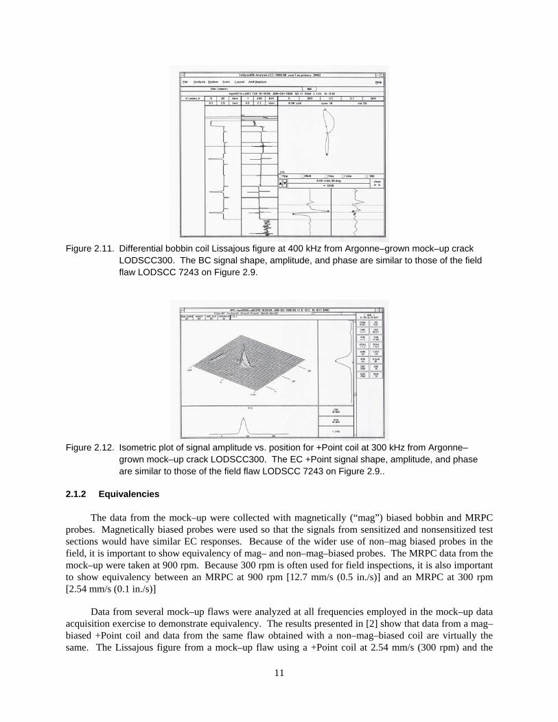
Figure 2.11. Differential bobbin coil Lissajous figure at 400 kHz from Argonne–grown mock–up crack

LODSCC300. The BC signal shape, amplitude, and phase are similar to those of the field flaw LODSCC 7243 on Figure 2.9.

Figure 2.12. Isometric plot of signal amplitude vs. position for +Point coil at 300 kHz from Argonne–

grown mock–up crack LODSCC300. The EC +Point signal shape, amplitude, and phase are similar to those of the field flaw LODSCC 7243 on Figure 2.9..

2.1.2 Equivalencies

The data from the mock–up were collected with magnetically (“mag”) biased bobbin and MRPC probes. Magnetically biased probes were used so that the signals from sensitized and nonsensitized test sections would have similar EC responses. Because of the wider use of non–mag biased probes in the field, it is important to show equivalency of mag– and non–mag–biased probes. The MRPC data from the mock–up were taken at 900 rpm. Because 300 rpm is often used for field inspections, it is also important to show equivalency between an MRPC at 900 rpm [12.7 mm/s (0.5 in./s)] and an MRPC at 300 rpm [2.54 mm/s (0.1 in./s)]

Data from several mock–up flaws were analyzed at all frequencies employed in the mock–up data acquisition exercise to demonstrate equivalency. The results presented in [2] show that data from a mag–biased +Point coil and data from the same flaw obtained with a non–mag–biased coil are virtually the same. The Lissajous figure from a mock–up flaw using a +Point coil at 2.54 mm/s (300 rpm) and the

11

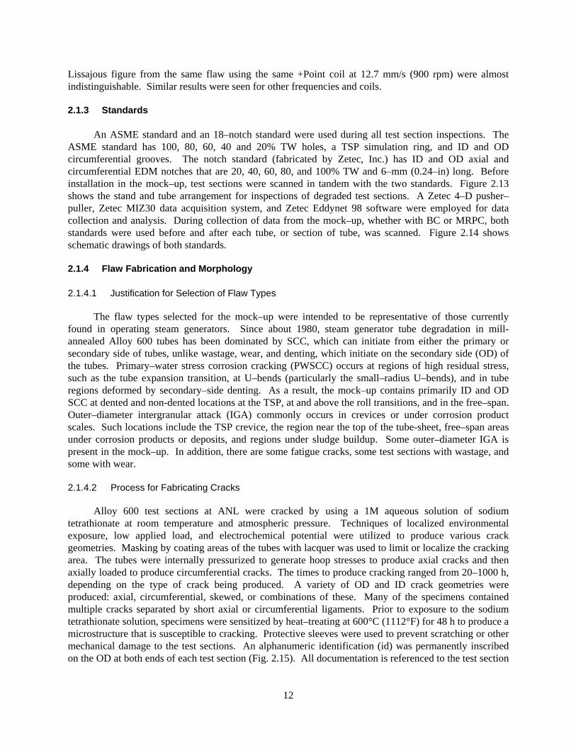
Lissajous figure from the same flaw using the same +Point coil at 12.7 mm/s (900 rpm) were almost indistinguishable. Similar results were seen for other frequencies and coils.

2.1.3 Standards

An ASME standard and an 18–notch standard were used during all test section inspections. The ASME standard has 100, 80, 60, 40 and 20% TW holes, a TSP simulation ring, and ID and OD circumferential grooves. The notch standard (fabricated by Zetec, Inc.) has ID and OD axial and circumferential EDM notches that are 20, 40, 60, 80, and 100% TW and 6–mm (0.24–in) long. Before installation in the mock–up, test sections were scanned in tandem with the two standards. Figure 2.13 shows the stand and tube arrangement for inspections of degraded test sections. A Zetec 4–D pusher–puller, Zetec MIZ30 data acquisition system, and Zetec Eddynet 98 software were employed for data collection and analysis. During collection of data from the mock–up, whether with BC or MRPC, both standards were used before and after each tube, or section of tube, was scanned. Figure 2.14 shows schematic drawings of both standards.

2.1.4 Flaw Fabrication and Morphology

2.1.4.1 Justification for Selection of Flaw Types

The flaw types selected for the mock–up were intended to be representative of those currently found in operating steam generators. Since about 1980, steam generator tube degradation in mill-annealed Alloy 600 tubes has been dominated by SCC, which can initiate from either the primary or secondary side of tubes, unlike wastage, wear, and denting, which initiate on the secondary side (OD) of the tubes. Primary–water stress corrosion cracking (PWSCC) occurs at regions of high residual stress, such as the tube expansion transition, at U–bends (particularly the small–radius U–bends), and in tube regions deformed by secondary–side denting. As a result, the mock–up contains primarily ID and OD SCC at dented and non-dented locations at the TSP, at and above the roll transitions, and in the free–span. Outer–diameter intergranular attack (IGA) commonly occurs in crevices or under corrosion product scales. Such locations include the TSP crevice, the region near the top of the tube-sheet, free–span areas under corrosion products or deposits, and regions under sludge buildup. Some outer–diameter IGA is present in the mock–up. In addition, there are some fatigue cracks, some test sections with wastage, and some with wear.

2.1.4.2 Process for Fabricating Cracks

Alloy 600 test sections at ANL were cracked by using a 1M aqueous solution of sodium tetrathionate at room temperature and atmospheric pressure. Techniques of localized environmental exposure, low applied load, and electrochemical potential were utilized to produce various crack geometries. Masking by coating areas of the tubes with lacquer was used to limit or localize the cracking area. The tubes were internally pressurized to generate hoop stresses to produce axial cracks and then axially loaded to produce circumferential cracks. The times to produce cracking ranged from 20–1000 h, depending on the type of crack being produced. A variety of OD and ID crack geometries were produced: axial, circumferential, skewed, or combinations of these. Many of the specimens contained multiple cracks separated by short axial or circumferential ligaments. Prior to exposure to the sodium tetrathionate solution, specimens were sensitized by heat–treating at 600°C (1112°F) for 48 h to produce a microstructure that is susceptible to cracking. Protective sleeves were used to prevent scratching or other mechanical damage to the test sections. An alphanumeric identification (id) was permanently inscribed on the OD at both ends of each test section (Fig. 2.15). All documentation is referenced to the test section

12

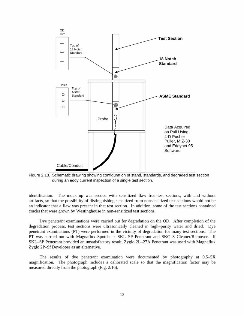
Cable/Conduit

Test Section

18 NotchStandard

ASME Standard

Data Acquired�on Pull Using�4-D Pusher�Puller, MIZ-30�and Eddynet 95�Software

Probe

Top of�18 Notch�Standard

OD�Circ

Top of�ASME�Standard

Holes

Figure 2.13. Schematic drawing showing configuration of stand, standards, and degraded test section

during an eddy current inspection of a single test section.

identification. The mock–up was seeded with sensitized flaw–free test sections, with and without artifacts, so that the possibility of distinguishing sensitized from nonsensitized test sections would not be an indicator that a flaw was present in that test section. In addition, some of the test sections contained cracks that were grown by Westinghouse in non-sensitized test sections.

Dye penetrant examinations were carried out for degradation on the OD. After completion of the degradation process, test sections were ultrasonically cleaned in high–purity water and dried. Dye penetrant examinations (PT) were performed in the vicinity of degradation for many test sections. The PT was carried out with Magnaflux Spotcheck SKL–SP Penetrant and SKC–S Cleaner/Remover. If SKL–SP Penetrant provided an unsatisfactory result, Zyglo 2L–27A Penetrant was used with Magnaflux Zyglo 2P–9f Developer as an alternative.

The results of dye penetrant examination were documented by photography at 0.5–5X magnification. The photograph includes a calibrated scale so that the magnification factor may be measured directly from the photograph (Fig. 2.16).

13

Figure 2.14. Schematic drawing of ASME (top) and 18–notch standard (bottom) used when scanning

degraded test sections and mock–up tubes.

14

Figure 2.15. Inscribed identification of tube specimen.

Figure 2.16. Dye penetration examination of tube specimen SGL865 showing an LODSCC.

Cross–sectional microscopy was performed on metallographically polished surfaces of many samples to provide documentation of the mock–up crack morphology. Figure 2.17 shows examples of LODSCC. The specimens were sometimes etched to delineate grain boundaries and other microstructural features, by electrolytic etching in 5% nitric acid–alcohol solution at 0.1 mA/mm2 for 5–30 seconds. The etching may enhance contrast of the image, but the tip of a tight intergranular crack can still be confused with a grain boundary. Photographic images were recorded at 10–500X magnifications.

About 50 of the cracks in the mock–up were provided by PNNL and produced by Westinghouse using a proprietary, doped–steam method. Axial and circumferential cracks, both ID and OD, were produced for the free–span, TSP, and roll transitions. Several IGA specimens, as well as fatigue and wastage samples, were also provided by PNNL. Figure 2.18 shows sketches of dye penetrant images for ODSCC specimens provided by PNNL for the mock–up.

15

(a) (b) Figure 2.17. Cross–sectional optical metallography for (a) branched LODSCC and (b) LODSCC.

2.1.4.3 Matrix of Flaws

Table 2.2 shows the distribution of flaw types in the mock–up. The flaw depths are distributed into three ranges, 0–50% TW, 51%–80% TW, and 81–100% TW. The distribution was intentionally skewed toward deeper cracks. This was intentional, to increase confidence in the POD values for deep cracks. Draft Regulatory Guide 1074 (“Steam Generator Tube Integrity”) describes criteria for performance demonstrations to quantify defect detection performance (POD for a given defect). The distribution of flaw sizes for the round–robin is not as uniform as suggested in Draft Regulatory Guide 1074, but other criteria involving extraneous signals, signals from fabricated defects, and detection and false calls have been met for the most part.

2.1.4.4 Crack Profiles by Advanced Multiparameter Algorithm and Comparison to Fractography

As part of the development of the multiparameter algorithm, the predictions of the algorithm have been compared to fractographic results on a wide variety of SCC cracks and EDM and laser notches. To provide an objective benchmark, however, blind–tests, in which the NDE estimates of the profiles were made without knowledge of the fractographic results, were performed.

The stress corrosion cracks for the blind tests were produced using the same techniques used to create the mock-up test sections (immersion in 1M aqueous solutions of sodium tetrathionate). A variety of OD and ID crack geometries were produced: axial, circumferential, skewed, and combinations of these. Many of the specimens contained multiple cracks separated by short axial or circumferential ligaments. The cracked tubes were examined using dye penetrant techniques, eddy current NDE, and destructive methods. The procedures for obtaining the data and the results are discussed below.

2.1.4.4.1 Procedures for Collecting Data for Multiparameter Analysis

The data collection procedures for inspection of the mock–up tubes are described in Section 2.2.2.2. These guidelines define the instrumentation setup (coil excitation frequencies, gain setting, cable length, sampling rate, probe speed, etc.) and calibration procedures for a given probe (e.g., bobbin, rotating,

16

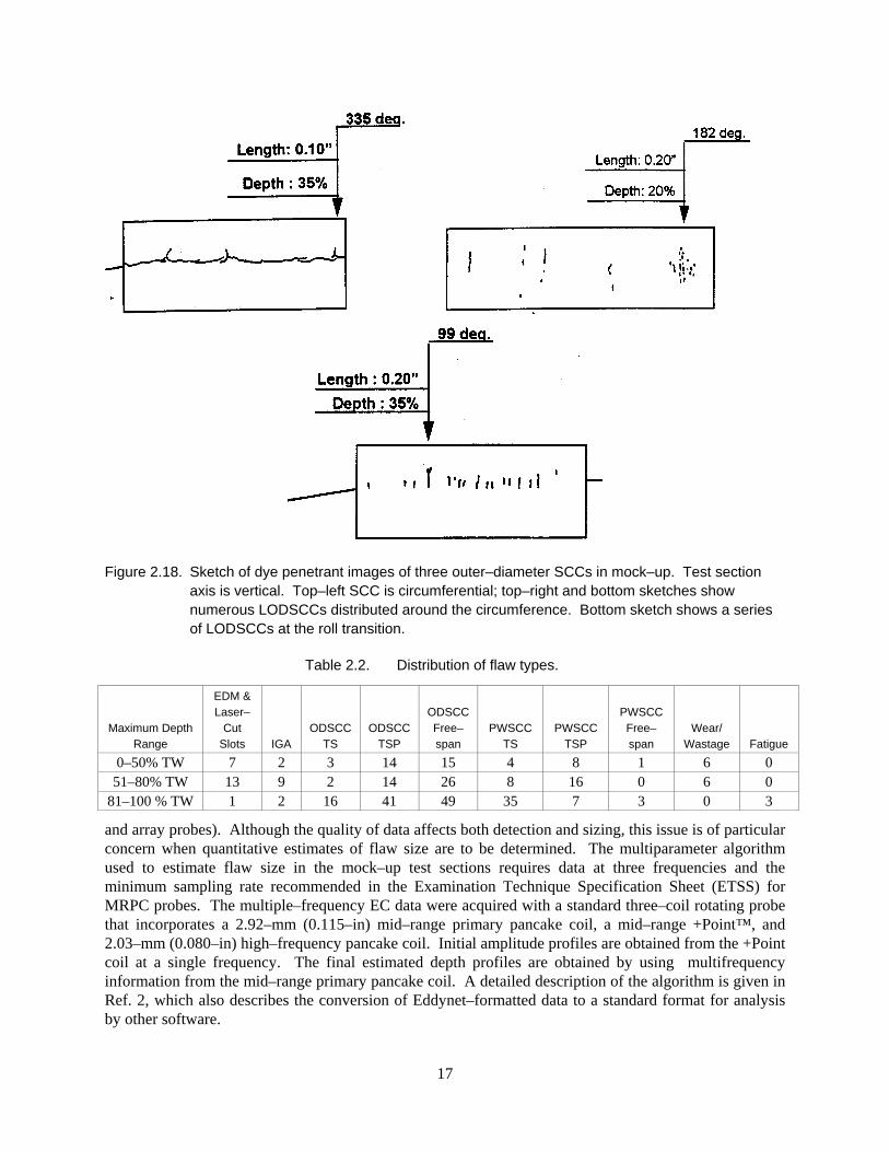
Figure 2.18. Sketch of dye penetrant images of three outer–diameter SCCs in mock–up. Test section

axis is vertical. Top–left SCC is circumferential; top–right and bottom sketches show numerous LODSCCs distributed around the circumference. Bottom sketch shows a series of LODSCCs at the roll transition.

Table 2.2. Distribution of flaw types.

Maximum Depth Range

EDM & Laser–

Cut Slots IGA

ODSCC TS

ODSCC TSP

ODSCC Free–span

PWSCC TS

PWSCC TSP

PWSCC Free–span

Wear/ Wastage Fatigue

0–50% TW 7 2 3 14 15 4 8 1 6 0 51–80% TW 13 9 2 14 26 8 16 0 6 0

81–100 % TW 1 2 16 41 49 35 7 3 0 3

and array probes). Although the quality of data affects both detection and sizing, this issue is of particular concern when quantitative estimates of flaw size are to be determined. The multiparameter algorithm used to estimate flaw size in the mock–up test sections requires data at three frequencies and the minimum sampling rate recommended in the Examination Technique Specification Sheet (ETSS) for MRPC probes. The multiple–frequency EC data were acquired with a standard three–coil rotating probe that incorporates a 2.92–mm (0.115–in) mid–range primary pancake coil, a mid–range +Point™, and 2.03–mm (0.080–in) high–frequency pancake coil. Initial amplitude profiles are obtained from the +Point coil at a single frequency. The final estimated depth profiles are obtained by using multifrequency information from the mid–range primary pancake coil. A detailed description of the algorithm is given in Ref. 2, which also describes the conversion of Eddynet–formatted data to a standard format for analysis by other software.

17

2.1.4.4.2 Fractography Procedures

For the destructive examination, the samples were heat–tinted before fracture to permit differentiation of the SCC and fracture opening surfaces. The specimens were then chilled in liquid nitrogen, and cracks were opened by fracture. Individual pieces of the specimen resulting from fracture are clearly identified, marked with new IDs, and documented. The fracture surfaces were examined macroscopically and with optical and scanning electron microscopy. The fractography and NDE data were digitized to obtain tabular and graphical comparisons of the depths as a function of axial or circumferential position. Well–defined markers on the test sections provided a means to accurately overlap the profiles.

The fractured surfaces were recorded by digital photography at a 0.2–10X magnification (Fig. 2.19). The method of illuminating the fracture surface plays an important role in obtaining the optimal image quality of the degradation. Optimal illumination was found by a trial–and–error method. For lagers crack, photographs may be taken at points along the fracture surface, and then a whole composite photograph be constructed later. All digital photographs have been identified with a unique file name that is traceable to a particular degradation mode and tube.

2.1.4.4.3 Procedure for Comparing Multiparameter Results to Fractography

Crack profiles were obtained by digitizing the photographs of the fracture surfaces and drawing lines through the points. The sampling distance depends on the complexity of the crack geometry. Short sampling distances were used for complicated geometries, while longer distances were used for simpler geometries, e.g., straight line or smooth contours. Fractography and NDE results were plotted in the same figure for comparative purposes (e.g., see Fig. 2.20). Lines were drawn through the EC data points to generate the NDE profiles (there were nominally 12 data points per centimeter [30 data points per inch] around the circumference and 30 data points per inch axially). The NDE and fractography profiles were then compared at many axial and circumferential positions, and the differences were used to establish the NDE uncertainty as a function of depth. The NDE uncertainties were then used to help assess the uncertainty in the POD curves presented in the report.

Figure 2.19. Fractography of tube specimen SGL413.

18

0.00

20.00

40.00

60.00

80.00

100.00

120.00

-2 0 2 4 6 8 10 12

EC NDEFractography

Dep

th (

%T

W)

Crack Length (mm)

Figure 2.20. Sizes and shapes of LODSCCs in tube specimen AGL 536 determined by EC NDE using the multiparameter algorithm (dotted curve) and fractography (smooth curve).

2.1.4.4.4 Comparison of Multiparameter Profiles with Fractography for Laboratory Samples

Initially, a set of 23 SCC was produced, which formed the basis for the initial assessment of the accuracy of the algorithm. Following the completion of the RR analysis, an additional 13 specimens from the mock–up were examined. Figures A1–A30 of Appendix A show profiles obtained from the multiparameter algorithm compared with those determined by fractography.

Figures 2.21a and 2.21b compare the maximum depths determined by destructive analysis with the predictions of the multiparameter algorithm for the initial set of 23 cracks and for all 36 cracked specimens. Linear regression fits and 95% confidence bounds for the observed data as a function of the multiparameter estimates are shown in the figures. The multiparameter model appears to do better at predicting the depths of deeper cracks. It also generally underestimates crack depths, a trend which is most pronounced for shallow cracks. This is not surprising. Because cracks are tighter near the crack tip, the signal from the deeper region is smaller and more difficult to characterize. Similarly, shallow cracks are very tight and have correspondingly smaller signals, and hence, again, are more difficult to characterize.

The least square fits from the set of 23 cracks and the set of 36 cracks are compared in Fig. 2.21c. The correlations are essentially identical and the estimate of the uncertainty in the depths predicted by the multiparameter algorithm is essentially unchanged by the addition of the 13 samples.

The least square fits can be used together with the direct estimate of the depth from the multiparameter method to get a better estimate of the error in the depth measurement. The overall root mean square error (RMSE) in the maximum depths given directly by the multiparameter method is 12.2%. The overall root mean square error (RMSE) in the adjusted predicted maximum depths using the fit in Fig. 2.21b is 8.6%. If the comparison is limited to deeper cracks, the RMSE is smaller, 8.0% for depths 50–100%, and 5.7% for outer–diameter SCCs of depths 80–100%. There are not enough data, however, to determine whether the apparent variation of the RMSE with depth is statistically significant.

Because the field of view of the rotating pancake probe is small, the depth measurements at points ≥ 5 mm apart along the crack profile are essentially independent, and additional comparisons of the estimated depth with that determined by fractography were made at various points along the crack profile for the cracks in the initial sample set. To avoid observer bias in the selection of the data used in this comparison, the intersections of the crack profiles with the major grid lines in the graphs of the

19

superimposed profiles were chosen as the points for the comparison. This corresponds, in most cases, to a spacing of 5 to 10 mm between points. Figures 2.22 show the results for 89 points from 23 different cracks, axial and circumferential, ID and OD. A linear regression curve and 95% confidence bounds for the observed data as a function of the multiparameter estimates are shown. The intercept in Fig. 2.22 is 13.8, somewhat less than that generated from the maximum depth data, i.e., there is a shift in the predicted values based on maximum depth and those based on points on the profile, but the slope of 0.78 is similar to the linear regression line slopes for the maximum depth data. In Fig. 2.23, the maximum depths for the initial set of 23 cracks as determined by phase analysis of +Point data are compared with the fractographic results. The regression line is close to that obtained from analysis of the maximum depth in terms of the multiparameter estimate of depth shown in Fig. 2.21, but there is greater scatter in the results.

Many NDE techniques were evaluated before selecting the multiparameter algorithm to estimate flaw sizes in the mock-up. The evaluated techniques include phase analysis of +Point data, multivariate regression analysis of EC data, multiparameter analysis of EC data with neural networks, high–frequency ultrasonics (UT) from the OD, Lamb waves, acoustic microscopy, and a combination of UT and EC data (from the ID). The multiparameter algorithm provided the most accurate estimate of crack sizes. A set of 20 test sections with cracks produced by a doped–steam technique were analyzed with the multiparameter algorithm and destructively analyzed by PNNL in an exercise carried out before the set of 23 test sections was evaluated. The NDE results from this set provided data for the development of the multiparameter

(a) (b)

Figure 2.21. Comparison of maximum depths determined by the multiparameter algorithm with that determined by fractography (a) set of 23 cracks; (b) set of 36 cracks; (c) comparison of the best fits to the two sets.

(c)

20

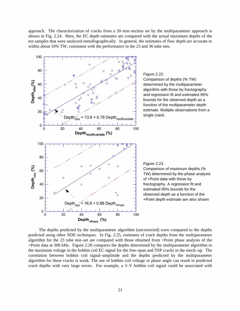
approach. The characterization of cracks from a 20–test–section set by the multiparameter approach is shown in Fig. 2.24. Here, the EC depth estimates are compared with the actual maximum depths of the ten samples that were analyzed metallographically. In general, the estimates of flaw depth are accurate to within about 10% TW, consistent with the performance in the 23 and 36 tube sets.

Figure 2.22. Comparison of depths (% TW) determined by the multiparameter algorithm with those by fractography and regression fit and estimated 95% bounds for the observed depth as a function of the multiparameter depth estimate. Multiple observations from a single crack.

Figure 2.23. Comparison of maximum depths (% TW) determined by the phase analysis of +Point data with those by fractography. A regression fit and estimated 95% bounds for the observed depth as a function of the +Point depth estimate are also shown

The depths predicted by the multiparameter algorithm (uncorrected) were compared to the depths predicted using other NDE techniques. In Fig. 2.25, estimates of crack depths from the multiparameter algorithm for the 23 tube test–set are compared with those obtained from +Point phase analysis of the +Point data at 300 kHz. Figure 2.26 compares the depths determined by the multiparameter algorithm to the maximum voltage in the bobbin coil EC signal for the free–span and TSP cracks in the mock–up. The correlation between bobbin coil signal–amplitude and the depths predicted by the multiparameter algorithm for these cracks is weak. The use of bobbin coil voltage or phase angle can result in predicted crack depths with very large errors. For example, a 3–V bobbin coil signal could be associated with

21

0

20

40

60

80

100

0 20 40 60 80 100

LODSCCCODSCCM

axim

um

Dep

th f

rom

M

ult

ipar

amet

er A

lgo

rith

m (

%T

W)

Maximum Depth from DE (%TW)

Two Points

Figure 2.24. Comparison of maximum depth determined by the multiparameter algorithm with metallographic results for the ten specimens that were destructively analyzed. Destructive evaluation (DE) was carried out using metallographic sectioning techniques.

0

20

40

60

80

100

0 20 40 60 80 100

LODSCC

CODSCC

LIDSCC

CIDSCC

Mu

ltip

aram

eter

Max

imu

m D

epth

(%

TW

)

+Point Phase Maximum Depth (%TW)

Figure 2.25. Estimates of maximum crack depths by the multiparameter algorithm compared with estimates using +Point phase analysis at 300 kHz.

Figure 2.26. Maximum bobbin coil voltage as a function of maximum crack depth for FS and TSP SCC in the mock-up. The eddy current multiparameter algorithm was used to profile the crack and determine the maximum depth.

0

5

10

15

20

25

30

0 20 40 60 80 100

TS

P FS

BC Voltage (volts)

Max Depth (multiparameter %TW)

22

Cracks of depths ranging from 25–100% TW. The correlation between bobbin coil phase angles and the depths predicted by the multiparameter algorithm for TSP cracks is also weak, as can be seen in Fig. 2.27 for LODSCC and in Fig. 2.28 for LIDSCC.

0

50

100

150

200

0 20 40 60 80 1

Bo

bb

in C

oil

Ph

ase

An

gle

(d

eg.)

Max Depth of LODSCC at TSP (%TW)

00

Figure 2.27. Bobbin coil phase–angle as a function of maximum crack depth for LODSCC at TSPs in the mock-up. The eddy current multiparameter algorithm was used to profile the crack and determine the maximum depth.

0

50

100

150

200

0 20 40 60 80 1

Bo

bb

in C

oil

Ph

ase

An

gle

(d

eg.)

Max Depth of LIDSCC at TSP (%TW)00

Figure 2.28. Bobbin coil phase–angle as a function of maximum crack depth for mock–up TSP LIDSCC. The eddy current multiparameter algorithm was used to profile the crack and determine the maximum depth.

2.1.4.5 Sizing studies of crack profiles

The probability of detection will be correlated with maximum depth. Since sizing will be done based on the multiparameter algorithm, it is important to understand uncertainties associated with the depth estimates. The database used for this evaluation was the initial set of 23 cracks (see Figures A1-23). Instead of just the maximum depth estimates to quantify the uncertainty, multiple depth measurements from the crack profile were used as discussed in Section 2.1.4.4.3 (Figure 2.22). This increases the number of data points used in the evaluation and it covers a wider range of depths. Because of the limited field of view of the rotating probe, the conclusions from the analysis of this data are expected to be generally applicable to the maximum depth estimates used in developing the POD curves.

The RMSE values for various binned depth ranges, are presented in Tables 2.3 and 2.4. In Table 2.3, the depth ranges are given in terms of the fractographic depths. This is useful when assessing the capability

23

of the multiparameter algorithm for cracks of a certain depth. In Table 2.4, the depth ranges are given in terms of the predicted depths. This is more useful when assessing the uncertainty in estimates from the multiparameter algorithm. In Fig. 2.29, the RMS in depth (in % TW) is plotted as a function of maximum depth. In the graph it is assumed that the values in Table 2.3 are at the midpoint of the depth range. The variation is truncated at 5% and 95% throughwall.

Table 2.3. Comparison of RMSE for depth estimates by multiparameter algorithm as a function of fractographic crack depth.

Depth Range (% TW)

RMSE Crack Profiling (% TW)

0–20 10.7

20–40 16.5

40–60 15.8

60–80 14.7

80–100 11.0

Table 2.4. Comparison of RMSE for depth estimates by multiparameter algorithm (MV) and by regression fit in Fig. 2.22 as a function of predicted crack depth.

Depth Range (% TW)

RMSE Crack Depth Multiparameter

(% TW)

RMSE Crack Depth Multiparameter corrected

(% TW)

0–20 19.5 12.8

20–40 21.0 23.0

40–60 16.3 16.1

60–80 12.2 10.6

80–100 9.8 9.5

The overall RMSE for all cracks of all depths is 15.1%, but this value is somewhat misleading because of the significant variation in the RMSE with depth.

In Table 2.4, two sets of RMSE values are given: one is based on the values obtained directly from the multiparameter algorithm, and the other on “corrected” values obtained from the regression fit shown in Fig. 2.22. For the shallowest cracks, the “corrected” values give a significantly lower RMSE value, but when all the data are considered, the differences in the RMSE for corrected and uncorrected predictions are small. This finding indicates little systematic bias in the predictions of the multiparameter algorithm, i.e., the errors are random.

24

Figure 2.29. Standard deviation in percent throughwall as a function of predicted maximum depth.

The effect of uncertainty in depths on the POD curves if the multiparameter algorithm is used to determine the “true” state of the mock–up for the NDE round–robin is based on the results for the maximum depths shown in Fig. 2.21 for the multiparameter estimates and Fig. 2.23 for the +Point estimates. The variance is taken to be constant over the central 80% of the wall thickness and then to decrease linearly for very shallow and very deep cracks. For the multiparameter estimates the standard deviation over the central portion is taken as 0.089; for the +Point estimates it is taken as 0.17.

2.1.4.4.5 Characterization of Cracks in Terms of mp

Although the probability of detection is normally expressed in terms of the maximum depth of the crack, it is also useful to express POD in terms of a parameter that better characterizes the structural integrity of the tube. A useful parameter for this purpose is mp, which characterizes the strength of the remaining throughwall ligament of a part–through crack and is defined as:

m p p b

p sc , (1)

where pb is the bursting pressure of an unflawed tube, and psc is the ligament rupture pressure of a part–throughwall crack. The parameter mp can be interpreted as a stress multiplier that relates the stress in the ligament ahead of the crack to the stress in an unflawed tube under the same loading. Incorporating the effect of both crack depth and length, mp better characterizes the effect of a flaw on the integrity of a tube than does maximum depth, although for short cracks, ligament rupture may not correspond to tube burst. The crack may just “pop” through without increasing in length. For rectangular cracks, mp can be expressed as a function of the crack and tube geometries by using the correlation [4]:

m p 1

amh

1ah

, (2a)

25

1 0.9a

h

2

11

m

, (2b)

where a = crack depth, h = wall thickness of tube, and m = bulging parameter [4].

Although Eqs. 1 and 2a–b can be used to estimate pressure for the tip ligament rupture of rectangular part–throughwall cracks, they are not directly applicable to SCC cracks, which can be irregular in shape and have variable depths along their lengths. Instead of being a single planar crack, they may be composed of a family of crack segments in different planes.

Currently, no widely accepted models are available for predicting the ligament rupture pressure of cracks with such complex geometries. Based on a plastic limit-load analysis viewpoint, it can be argued that the collapse behavior of a crack tip ligament with an irregular point–by–point variation of crack depth should be similar to a crack with a smoothed–out, “average” profile for crack depth. Although the real crack may have short throughwall segments at a number of locations, from the standpoint of plastic collapse of the ligament, the tube behaves as if it has a smoothly varying average ligament thickness (or crack depth) profile. Thus, we assume that the average profile measured by the EC method, which gives a smoothed–out, “average” profile, can be used for the analysis of the flaw.

Because the measured crack depth profile by the ANL multifrequency EC algorithm is generally not rectangular, the following procedure was used to establish the length and depth of an equivalent rectangular crack [4]:

Choose a crack depth do and assume that any crack segment with depth d < do does not adversely affect the crack tip ligament rupture pressure of the tube (Fig. 2.30a). In other words, replace the original crack depth profile by a new crack depth profile in which any crack segment with depth d < do is replaced by d = 0 (Fig. 2.30b). The choice of do fixes the length of the candidate equivalent rectangular crack (Lo).

Determine the depth of the candidate equivalent rectangular crack by equating its area to the area under the crack depth profile defined in step 1 (Fig. 2.30b). For example, in Figs. 2.30a–b, the choice of do = 50% fixes the length and depth of the candidate equivalent rectangular crack at 9 mm and 70%, respectively.

Generate a series of candidate equivalent rectangular cracks by parametrically varying do and calculate the ligament rupture pressures for all the candidates (Fig. 2.31). The final equivalent rectangular crack corresponds to the candidate with the lowest ligament rupture pressure (Fig. 2.31).

26

-20

0

20

40

60

80

100

-10 -5 0 5 10

Cra

ck D

epth

(%

TW

)

Relative Axial Position (mm)

do

-20

0

20

40

60

80

100

-10 -5 0 5 10

Cra

ck D

epth

(%

TW

)

Relative Axial Position (mm)

do

Candidateequivalentrectangularcrack

(a) (b) Figure 2.30. (a) Crack depth profile measured by eddy current and (b) a candidate equivalent

rectangular crack corresponding to depth do = 50% and Lo = 10 mm (0.39 in).

15

20

25

30

35

40

45

0.5 0.6 0.7 0.8 0.9 1

11mm9 mm7 mm

Liga

men

t Fai

lure

Pre

ssur

e (M

Pa)

Crack Depth (a/h)

Figure 2.31. Ligament rupture pressures corresponding to three candidate equivalent rectangular cracks, 11 mm (0.43 in) by 60%, 9 mm (0.35 in) by 70%, and 7 mm (0.28 in) by 75%. The equivalent rectangular crack is 9 mm (0.35 in) by 70% because these values correspond to the lowest ligament rupture pressure (30 MPa or 4.35 ksi).

This procedure has been automated by systematically choosing various candidate equivalent crack lengths Lo (instead of do), determining the corresponding candidate equivalent crack depths, and selecting the equivalent crack length, depth, and value of mp that correspond to the minimum ligament rupture pressure.

2.1.4.6 Reference–State Summary Table for Mock–up

Tables B1 and B2 of Appendix B summarize information about the flaws in the mock-up. The flaw type, BC volts, BC phase, whether ID or OD, three–letter code for the flaw, maximum depth as determined by multiparameter algorithm, flaw length, average depth area, and mp are all included in the flaw table. Not shown are flaw location in the mock–up (row, column, and level) and beginning and end points of the flaw, in BC data points. The test sections included in the tables are those for which mp was determined. As a result, these tables present data from the flaws that have relatively large EC signals, permitting the profiling to be carried out accurately and leading to an accurate value of mp. Table B1 shows the values for TSP SCC, while Table B2 shows the values for free–span SCC.

27

2.2 Design and Organization of Round–Robin

A very important aspect of developing the round–robin (RR) exercise was input from an NDE Task Group. The Task Group helped define the parameters found in a field inspection and provided input on how to ensure that the RR mimicked an in–service inspection (ISI). Members of the Task Group were from utilities, vendors, EPRI, NRC, and ANL. The industry members were G. Henry and J. Benson (EPRI), T. Richards and R. Miranda (FTI), D. Adamonis and R. Maurer (Westinghouse), D. Mayes (Duke Engineering and Services), S. Redner (Northern States Power), and B. Vollmer and N. Farenbaugh (Zetec).

The Task Group provided input related to the makeup of the mock–up, the quality of the data collected for the RR, the nature of the flaws, procedures for analyzing data, and documentation. The Task Group helped meet the goal of providing an RR exercise that represents, as closely as possible, a true field inspection. The Task Group provided input on the analysis guidelines, data acquisition, degradation assessment, training manual, and examination technique specification sheets (ETSSs). The RR began only after the Task Group approved the documentation used for the RR and concluded that flaws in the mock–up had EC signals similar to those observed under field conditions. In addition, opinions were expressed on the handling of rotating probe spin calls, the handling of the logistics of distributing EC data to the various teams, the content of the training documentation, the makeup of the analysis team, and the equivalency demonstrations needed. Because of input from the Task Group on the makeup of the analysis teams, a decision was made to use a five–member team that would include a primary, a secondary, and two equally qualified resolution analysts to analyze the EC data. The fifth member, the independent qualified data analyst (QDA), would be from a utility. The primary and secondary analysts were to report their observations independently of each other. The resolution analysts would review calls when the primary and secondary analysts’ calls differed. The independent QDA uses his judgment to monitor the effort, looking for excess overcalls and reviewing a sample of 40 test sections to ascertain if flaws are being missed.

2.2.1 The Mock–up as ANL’s Steam Generator

The mock–up was treated as though it were a steam generator owned by a utility. The role of the utility in this case was taken by ANL. The ISI followed the process and procedures used by industry. ANL was responsible for preparing documentation, monitoring data collection, monitoring data analysis, and carrying out statistical analysis.

2.2.1.1 Responsibilities

2.2.1.1.1 Data Collection

Data were collected by a qualified (according to EPRI guidelines) team from Zetec in June and again in August 1999. A qualified observer from Westinghouse was also present. The data acquisition team included a QDA Level II and a QDA Level IIIa.

2.2.1.1.2 NDE Task Group

The NDE Task Group provided input on data collection during the development of the documentation. They also provided input on how to carry out the degradation assessment, how to select the ETSS, how to carry out the site–specific examinations, and how to prepare the training manual. The role of the Task Group, in general, was to help ANL mimic a field inspection.

28

2.2.1.1.3 Analysis of Round–Robin

Analysts’ RR reports were collected from RR teams by ANL proctors and converted to Excel files so they could be analyzed in a convenient manner. Proctors (ANL staff) were present during all analysts’ activities to ensure that procedures developed for the analysis of data were followed correctly.

2.2.1.1.4 Statistical Analysis

The RR reports were analyzed at ANL. Statistical fits to the inspection results for POD as a function of crack depth and mp with confidence limits that include errors in reference state were developed. P. Heasler and R. Kurtz of PNNL provided assistance on the statistical analysis based on their experience with previous RR tests for NDE. Decisions regarding the grading unit for the statistical analysis were arrived at through discussions with P. Heasler.

2.2.1.1.5 Documentation

The documentation prepared included the degradation assessment, the appropriate ETSS, data collection procedures, analysis guidelines, and the training manual. Detailed documentation was prepared on how the RR exercise was carried out, the sequence of events, and the role of the ANL proctors, including administration of site–specific exams.

2.2.2 Round–Robin Documentation

Four documents were prepared for the mock–up testing and for the RR data analysis. They are ANL001 Rev. 3 “Argonne Analysis Guideline,” ANL002 Rev. 3 “Multifrequency EC Examination of Tubing within the ANL SG Mock–up,” ANL003 Rev. 3 “SG Mock–up Tubing Degradation Assessment and Technique Qualification,” and ANL004 Rev. 3 “Training Manual.” These documents are discussed below.

2.2.2.1 Degradation Assessment (ANL003 Rev. 3)

A “Steam Generator Tube Degradation Assessment” for flaws was prepared, per the requirements specified in NEI–97–06 and Revision 5 of the “EPRI PWR Steam Generator Examination Guidelines.” In accordance with Rev. 5 of the “EPRI PWR Steam Generator Examination Guidelines,” the EPRI–qualified techniques were reviewed to ensure that application of these techniques was pertinent to site–specific conditions of the mock–up.

This document identified the degradation mechanisms in the tubing of the steam generator mock–up. This assessment also identified the inspection methods to be used to ensure that the inspection techniques and personnel used for the detection and sizing of tube flaws are appropriate for all degradation mechanisms. The training document for the RR addressed the handling of anomalous signals.

The degradation assessment reviewed all types of degradation in the mock–up, including the following:

(a) Intergranular attack (IGA) is characterized by a uniform or relatively uniform attack of the grain boundaries over the surface of the tubing. When the occurrence is over a relatively large extent exhibiting three–dimensional features, the IGA is referred to as volumetric IGA. IGA is initiated at the outside surface of the tubing material. The IGA present in the mock–up is not mixed with SCC,

29

a combination that can be found in the field, which is easier to detect than pure IGA. However, the unmixed IGA in the mock–up is similar to that found in plants, such as Cook, Point Beach, and San Onofre.

(b) Primary–water stress corrosion cracking (PWSCC) describes the cracking that occurs on the primary side of tubes (the inside diameter) when a source of stress is present in a susceptible material. Locations of PWSCC in the mock–up include expansion transitions and dents.

(c) Wear is the volumetric removal of material caused by the mechanical action of one material in contact with another.

(d) Corrosive fatigue can result from the alternating stress cycles produced by tube vibration that may be accelerated by a corrosion process occurring during stress cycling. A few fatigue cracks can be found in the mock–up.

(e) Wastage is loss of material initiating at the outer wall of the tubing by corrosion.

(f) Outer diameter stress corrosion cracking (ODSCC) refers to a range of stress corrosion cracking morphologies observed to occur along the OD of Alloy 600 steam generator tubing. It is mainly found at the TSP, in the free–span, and in the tube-sheet.

2.2.2.2 Preparations for Examination Technique Specification Sheets (ETSSs)

The EPRI Appendix H EC techniques used to examine steam generator tubes were reviewed to determine their applicability to the site–specific mock–up conditions. The tube bundle degradation was investigated to support the Appendix H technique qualifications. Three classifications of EC techniques are available: “site–qualified,” “qualified,” and “nonqualified.”

“Site–qualified techniques” have an EPRI Examination Technique Specification Sheet (ETSS) for detection and/or sizing. Before development of the mock–up ETSSs, the essential variables for all EPRI–qualified techniques were reviewed. This procedure ensured that the applications of the EPRI techniques are pertinent to site–specific conditions for the mock–up steam generator.

The EPRI ETSSs have been reviewed for similarity and applicability to the mock–up conditions. For degradation previously “detected” in the mock–up, the EC signals have been compared to the EPRI signals to classify the technique as site–qualified. Damage mechanisms in the mock–up have site–qualified techniques for detection.

Two ETSSs were developed for the ANL mock–up. These ETSSs are the result of reviewing EPRI ETSSs for the various degradation mechanisms in the mock–up and combining them into two documents. The ETSSs for the round–robin are given in Appendix C.

2.2.2.3 Data Acquisition Documentation (ANL002 Rev. 3)

The document “Multifrequency EC Examination of Tubing within the ANL SG Mock–up” provides all information necessary to collect the RR data. The procedures mimic those of an actual ISI. The basis of the data acquisition is the ETSS. The document defines the frequencies, axial and rotational speeds, and calibration procedures.

30

All of the tubes were inspected over their full length with a bobbin coil. The EPRI site–qualified technique ETSS 96008, covered by ANL’s ETSS#1 (described later), was used. This technique has an EPRI–reported probability of detection of 85% at > 40% TW at a confidence level of 90% in those areas not associated with the roll transition.

The tubing in the mock–up steam generator was mechanically expanded (rolled) in the ANL shop. The transition zone is the region of the tube where the tube transitions from the expanded tube diameter to the nominal tube. Axial and circumferential indications are found in this region. All the tubes were inspected with a three–coil MRPC probe (Plus–Point, standard pancake and shielded high–frequency coil) at the top of the tube–sheet region. The EPRI site–qualified technique ETSS 96508, covered by mock–up ETSS#2, was used for detection of IDSCC in the tube-sheet. This technique has an EPRI–reported probability of detection of 84% at > 50% TW and a 90% confidence level for both axial and circumferential indications. The EPRI site–qualified technique ETSS 96403, covered by ANL’s ETSS#2 (described later), was used for the detection of ODSCC in the tube-sheet. This technique has an EPRI–reported probability of detection of 81% at > 50% TW and a 90% confidence level for both axial and circumferential indications.

Bobbin–coil indications at TSPs were investigated with a rotating coil (Plus–Point). The site–qualified bobbin technique for nondented TSPs is EPRI ETSS 96007, covered by mock–up ETSS#1. The EPRI–reported probability of detection is 89% at > 60% TW and a 90% level of confidence. For all rotating coil inspections, the site–qualified technique EPRI ETSS 96403, covered by mock–up ETSS#2, was used. This technique has an EPRI–reported probability of detection for axial and circumferential indications of 81% at > 50% TW and a 90% confidence level.

Corrosion of the TSPs causes the tubing to become dented, resulting in high localized stresses that lead to stress corrosion cracking. The EPRI site–qualified Technique ETSS 96012 (covered by mock–up ETSS#1) was used for bobbin detection of axial PWSCC at TSP intersections (dent < 2 V). This technique has an EPRI–reported probability of detection of 89% at > 34% TW and a confidence level of 90%. Site–qualified technique EPRI ETSS 96508 (covered by mock–up ETSS#2) was used for rotating coil detection of axial and circumferential PWSCC at dented locations and has an EPRI–reported probability of detection of 84% at > 50% TW and a confidence level of 90%.

Degradation due to wear is adequately identified by a bobbin coil examination. The technique used for detection of tube wear was EPRI ETSS 96004 (covered by mock–up ETSS#1) with an EPRI–reported probability of detection of 82% for > 50% TW and a 90% confidence level.

No special examination requirements are listed in the “EPRI PWR Steam Generator Examination Guidelines” for fatigue degradation due to the rapid growth rates associated with fatigue cracks, making them difficult to detect before they leak and become readily identifiable.+++

Note that the EPRI–reported PODs may be determined from small sample sets, with the lower confidence limit being the stated POD. As an example, if all cracks in a set of 11 test sections were detected (100% detection), the lower 90% confidence limit is 82%, and the stated POD would be 0.82. EPRI–stated PODs are adjusted to sample size.

2.2.2.3 ANL Analysis Guideline (ANL001 Rev. 3)

This procedure provided the technical direction for the performance of EC examinations of the ANL SG mock–up. It was followed by all examination personnel and mimics industry ISI guidelines. Flaws were located by data point. Percent throughwall and the three–letter codes for the flaw types were

31

recorded, with the exception of dents and dings. Data were reviewed for the presence of undesirable noise with the following criteria: (a) Undesirable system noise was determined by identifying electrical interference or spiking associated with faulty probes, cabling, and equipment. Studies have shown that probe wear can generate undesirable horizontal noise, resulting in poor signal–to–noise ratios. (b) Undesirable tube noise was determined by identifying signals caused by excessive permeability, pilgering, chatter, variations in tube geometry and tube cleanliness, and secondary–side sludge and deposits. These conditions were reported by the analyst so that a review could be performed to disposition these locations.

The primary and secondary analysts generated data used in the final analyst report and were responsible for reporting all indications. The resolution team (consisting of two resolution analysts and an independent QDA) performed the task of comparing and resolving discrepancies between the primary and secondary analyses. All identified differences in data interpretation were reviewed by resolution analysts to arrive at the final interpretation. The following procedures were used:

(a) If the primary and secondary analysts agreed that an indication is a flaw, it was reviewed by two resolution analysts. The independent QDA has the final say if there is no consensus on the call.

(b) If the primary and secondary analysts both give the “no detectable degradation” (NDD) call for a test section, there was no further analysis.

(c) If the primary and secondary analysts disagreed, the disagreement was resolved by the two resolution analysts. If the resolution analysts were not in agreement, the independent QDA made the final call.

Table 2.5 shows an example of the data recorded by the analysts. The row and column of the test section was entered along with the voltage, phase angle, percentage TW, EC analysis channel (CH), location by data point, three–letter code, and whether ID or OD.

2.2.2.4 Training Manual (ANL004 Rev. 3)

A training manual was developed for the analysts to read before the RR exercise. The manual was intended to provide a level of information about the mockup similar to that which would be provided for an industry inspection. The information provided included a schematic diagram, a listing of type of artifacts present, a discussion regarding the presence of the circumferential markers, a discussion of how the data for the RR were acquired, and a table showing the format for entering data. It also describes the types of degradation that could be present: LODSCC and CODSCC at the top of the tube-sheet (TTS) with and without sludge; LODSCC at TSPs and in the free–span; CODSCC in the free–span; PWSCC at dented TSPs and at the top of the tube-sheet with and without sludge; free–span dings with and without LIDSCC, fatigue cracks; and IGA. Examples of mock–up bobbin coil data (Eddynet 98 line traces and Lissajous figures), followed by MRPC data (isometric plots) for the various types of flaws present, were provided.

2.2.2.5 Preparations for Examination Technique Specification Sheets (ETSSs)

The EPRI Appendix H EC techniques used to examine steam generator tubes were reviewed to determine their applicability to the site–specific mock–up conditions. The tube bundle degradation was investigated to support the Appendix H technique qualifications. Three classifications of EC techniques are available: “site–qualified,” “qualified,” and “nonqualified.”

32

Table 2.5. Example format for entering data

SG ROW COL VOLTS DEG % TW CH LOC (Data Point)

UTIL 1 UTIL 2

1 F 19 4.23 174 0 P1 +2383 DNT OD

11 B 20 3.67 110 50 P 1 +2578 DSI OD

11 B 15 1.31 13 33 P 1 +3789 NQI ID

11 C 14 0.32 109 52 P 1 +3299 NQI OD

11 D 3 3.1 180 0 P 1 +2678 DNT

11 E 8 1.51 125 30 P 1 +2276 NQI OD

11 F 6 2.36 88 68 6 +6578 ADI OD

11 E 7 2.98 181 0 P 1 +2386 DNG

11 G 13 4.56 125 30 P 1 +2768 DTI OD

11 E 8 2.61 89 66 6 +3287 VOL OD

11 A 15 1.76 76 80 P2 +2367 SCI ID

11 I 17 2.67 89 66 6 +987 SAI OD

11 G 11 4.7 105 50 6/P +1224 MVI OD

11 A 5 3.8 98 40 P2 +3398 MCI OD

11 D 3 1.6 15 40 P1 +2688 DNI ID

11 B 22 3.45 76 80 6 +3267 MAI OD

“Site–qualified techniques” have an EPRI Examination Technique Specification Sheet (ETSS) for detection and/or sizing. Before development of the mock–up ETSSs, the essential variables for all EPRI–qualified techniques were reviewed. This procedure ensured that the applications of the EPRI techniques are pertinent to site–specific conditions for the mock–up steam generator.

The ETSSs have been reviewed for similarity and applicability to the mock–up conditions. For degradation previously “detected” in the mock–up, the EC signals have been compared to the EPRI signals to classify the technique as site–qualified. Damage mechanisms in the mock–up have site–qualified techniques for detection. The ETSSs for the round–robin are given in Appendix C.

2.2.3 Acquisition of Eddy Current Mock–up Data and Description of Data Acquisition Documentation

The qualified Level II Operator was responsible for acquiring examination data and for the quality of that data. This Operator reviewed all calibrations performed, for acceptance. The Level III Examiner was responsible for all aspects of the examination task: establishing the essential variables for the examination, approving the procedures to be used and making changes when required, recommending the appropriate examination technique(s), providing judgment on data quality issues, resolving analysis discrepancies, and evaluating data.

33

The equipment used for data acquisition was the Zetec MIZ–30(A) Digital Multi–frequency Eddy Current Instrument used with Zetec Eddynet Software for data acquisition and analysis. The electronic instrumentation of the EC system was certified. A Hewlett–Packard computer, configured to operate the EC instrument and associated controllers and fixtures, was used for data acquisition. Removable–media data storage devices, such as optical disk drives and disks, of a type compatible with the EC system and operating software were used.

The EC probes were specified on the appropriate technique sheets. For each examination, the manufacturer, a description or part number, type, and size and length of probe used were reported on the summary form recorded with each calibration group. The calibration tube standards were manufactured from a length of tubing of the same nominal size and material type as that of the tubing examined. The tubing size and material type are listed on each technique sheet.

The inside surfaces of all tubes to be examined were as clean as practical and free of obstructions or other extraneous matter. For bobbin probe examination, the scan included the full length of each tube, unless specified differently in the inspection plan. For rotating–probe examination, the scan was as specified in the inspection plan. Bobbin–coil examination data were acquired during probe retraction (pull). Rotating probe data was acquired during either probe insertion or retraction (push or pull).

During June and August of 1999, a qualified three–person team from Zetec collected data from the mock–up (Fig. 2.32); an observer from Westinghouse was also present. The data acquisition team included a QDA Level IIa and a QDA Level IIIa. Data were acquired with a 10–D pusher–puller, MIZ30 with 36–pin cables, and Eddynet software. BC data from a mag–biased probe were collected from all 3600 test sections of the mock–up. The BC data were calibrated before and after the 4–h interval required to collect the data. No changes in voltage from the defects in the calibration standard were observed during this time period. A magnetically biased, rotating, three–coil probe that includes a +Point, 2.9–mm (0.115–in)–diameter pancake and high–frequency shielded coil was used to collect data from all 400 tube–sheet test sections and all special–interest (spin call) test sections. A comparison of magnetically biased and unbiased coils showed that biasing eliminates the voltage shift and noise in the +Point EC signal resulting from tube sensitization.

The BC data were taken at 0.53 m/s (21 in./s), maintaining a digitization rate of 15 samples/cm (37 samples per in). Bobbin coil data were taken at 400, 200, 100, and 20 kHz (differential and absolute). MRPC data were obtained from all degraded test sections and test sections with artifacts, as well as hundreds of test sections without flaws or artifacts. An ASME standard and a standard with 18 ID and OD axial and circumferential EDM notches (20, 40, 60, 80, and 100% TW) were used for calibration. MRPC data were taken at 900 rpm and an axial speed of 12.7 mm/s (0.5 in./s) to maintain a digitization rate of 12 samples/cm (30 samples per in) in the circumferential direction and 30 per in the axial direction. Data were taken at 600, 400, 300, 200, and 100 kHz. Nine +Point probes were used during this exercise because of probe wear. MRPC probes were replaced when one of the channels could not be nulled. This condition appears on the computer screen as an alert “flag.”

All data were recorded on 2.6–GB magneto–optical disks. Two copies of the master disk were made, and all the data were copied to an ANL computer backup system. The setup for the bobbin coil and +Point probe matches or exceeds the specifications of the ETSSs for the tube bundle.

The mock–up data collected by Zetec were analyzed at ANL (by ANL personnel) with Eddynet98 software. The locations of the flaw signals in the mock–up were checked against the assembly data for the mock–up. Locations of possible dings introduced during assembly of the mock–up were

34

noted. These dings could be created if a test section were inadvertently pressed against the simulated TSP during assembly.

During summer 1999, a recognized industry expert reviewed the bobbin coil data from the ANL steam generator mock–up and some of the MRPC data acquired by Zetec. The overall quality of the data was judged good, generally representative of field data, and meeting or exceeding requirements for qualified techniques.

35

Figure 2.32. Photograph of underside of tube bundle. Conduit carrying the EC probe is shown being

positioned under a tube.

36

2.2.4 Participating Companies and Organization of Team Members

Companies participating in the RR provided a list of analysts who would be available to participate. For those companies who supplied more names than would be needed, ANL selected the team members by random picks from the list provided. The team members were expected to be available during the entire exercise, generally seven to eight working days. Analysts were generally QDA Level IIa or III. The resolution analysts and independent QDAs were Level III or IIIa. During the RR exercise, the primary and secondary analysts did not communicate with each other or the resolution analysts. Upon submitting their reports, the primary and secondary analysts could discuss the reports with the resolution analysts, but the reports were not changed as a result. The resolution analysts provided the report used for establishing POD.

2.2.5 Review of Training Manual by Teams

Team members reviewed the training manual either the day before or the same day that the ANL proctor arrived with the mock–up data and site–specific tests. The analysts were able to review the types of degradation in the mock–up and typical EC signal responses. They also carefully reviewed the mock–up geometry and became familiar with the EC signal response from test–section ends, as well as from roll transitions, TSPs, and the run–out section of the mock–up. The analysts reviewed the reporting procedure and could ask the ANL staff questions related to the training manual.

2.2.6 Data Analysis Procedures and Guidelines

All flaw indications were to be evaluated. Indication types to be reported were characterized by the frequencies or frequency mixes that were qualified. For indication types to be reported in terms of depth, a means of correlating the indication depth with the signal amplitude or phase was established and based on the basic calibration. Flaw depth was reported in terms of percentage of loss of tube wall. For axial and circumferential flaws reported with MRPC, depth was determined from the “hit” that provides the greatest amplitude. For circumferential cracks, the maximum depth was determined from axial cuts through the crack. Reported indications of possible tube wall degradation were described in terms of the following, as a minimum:

(a) The location along the length of the tube with respect to the actual data point, as appropriate for the technique used. For MRPC data, the circumferential location was defined by the data point of the flaw called.

(b) The depth of the indication through the tube wall, when applicable.

(c) The signal amplitude.

(d) The frequency or frequency mix from which the indication was evaluated.

In addition to the ANL documents, the analysts were given an errata sheet with eight corrections and two procedure changes. The errata sheet indicated additional three letter codes to be used, clarifications regarding setting of span and inputting of data, and corrections to references in documentation provided. The changes involved clarification regarding how to input MRPC data for complex flaws (at a maximum, four indications were recorded for a given axial position) and a channel change for the voltage normalization of the high–frequency coil of the three–coil MRPC probe.

37

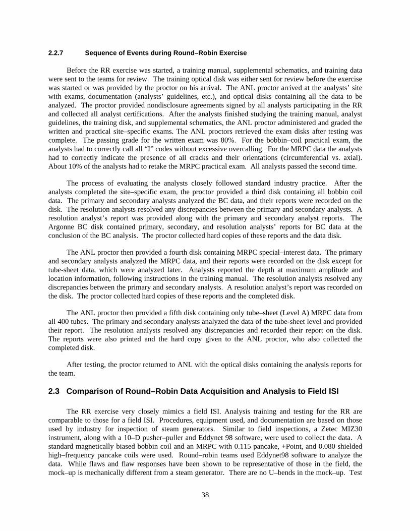
2.2.7 Sequence of Events during Round–Robin Exercise

Before the RR exercise was started, a training manual, supplemental schematics, and training data were sent to the teams for review. The training optical disk was either sent for review before the exercise was started or was provided by the proctor on his arrival. The ANL proctor arrived at the analysts’ site with exams, documentation (analysts’ guidelines, etc.), and optical disks containing all the data to be analyzed. The proctor provided nondisclosure agreements signed by all analysts participating in the RR and collected all analyst certifications. After the analysts finished studying the training manual, analyst guidelines, the training disk, and supplemental schematics, the ANL proctor administered and graded the written and practical site–specific exams. The ANL proctors retrieved the exam disks after testing was complete. The passing grade for the written exam was 80%. For the bobbin–coil practical exam, the analysts had to correctly call all “I” codes without excessive overcalling. For the MRPC data the analysts had to correctly indicate the presence of all cracks and their orientations (circumferential vs. axial). About 10% of the analysts had to retake the MRPC practical exam. All analysts passed the second time.

The process of evaluating the analysts closely followed standard industry practice. After the analysts completed the site–specific exam, the proctor provided a third disk containing all bobbin coil data. The primary and secondary analysts analyzed the BC data, and their reports were recorded on the disk. The resolution analysts resolved any discrepancies between the primary and secondary analysts. A resolution analyst’s report was provided along with the primary and secondary analyst reports. The Argonne BC disk contained primary, secondary, and resolution analysts’ reports for BC data at the conclusion of the BC analysis. The proctor collected hard copies of these reports and the data disk.

The ANL proctor then provided a fourth disk containing MRPC special–interest data. The primary and secondary analysts analyzed the MRPC data, and their reports were recorded on the disk except for tube-sheet data, which were analyzed later. Analysts reported the depth at maximum amplitude and location information, following instructions in the training manual. The resolution analysts resolved any discrepancies between the primary and secondary analysts. A resolution analyst’s report was recorded on the disk. The proctor collected hard copies of these reports and the completed disk.

The ANL proctor then provided a fifth disk containing only tube–sheet (Level A) MRPC data from all 400 tubes. The primary and secondary analysts analyzed the data of the tube-sheet level and provided their report. The resolution analysts resolved any discrepancies and recorded their report on the disk. The reports were also printed and the hard copy given to the ANL proctor, who also collected the completed disk.

After testing, the proctor returned to ANL with the optical disks containing the analysis reports for the team.

2.3 Comparison of Round–Robin Data Acquisition and Analysis to Field ISI

The RR exercise very closely mimics a field ISI. Analysis training and testing for the RR are comparable to those for a field ISI. Procedures, equipment used, and documentation are based on those used by industry for inspection of steam generators. Similar to field inspections, a Zetec MIZ30 instrument, along with a 10–D pusher–puller and Eddynet 98 software, were used to collect the data. A standard magnetically biased bobbin coil and an MRPC with 0.115 pancake, +Point, and 0.080 shielded high–frequency pancake coils were used. Round–robin teams used Eddynet98 software to analyze the data. While flaws and flaw responses have been shown to be representative of those in the field, the mock–up is mechanically different from a steam generator. There are no U–bends in the mock–up. Test

38

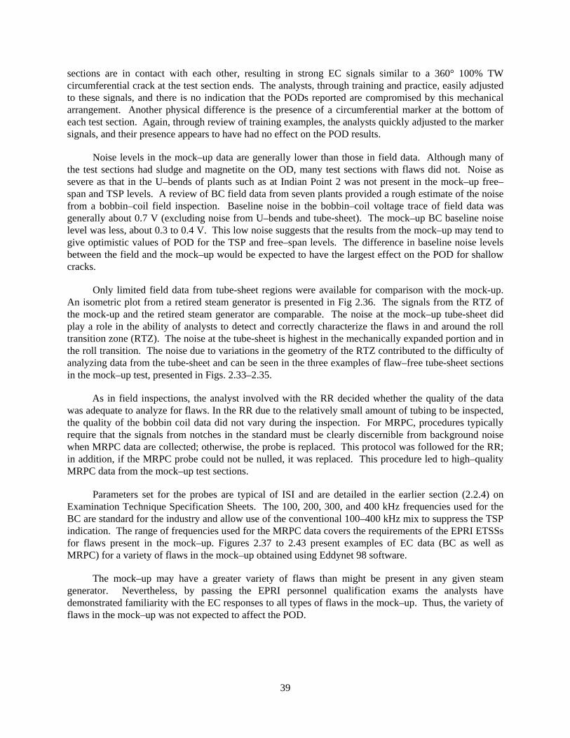
sections are in contact with each other, resulting in strong EC signals similar to a 360° 100% TW circumferential crack at the test section ends. The analysts, through training and practice, easily adjusted to these signals, and there is no indication that the PODs reported are compromised by this mechanical arrangement. Another physical difference is the presence of a circumferential marker at the bottom of each test section. Again, through review of training examples, the analysts quickly adjusted to the marker signals, and their presence appears to have had no effect on the POD results.

Noise levels in the mock–up data are generally lower than those in field data. Although many of the test sections had sludge and magnetite on the OD, many test sections with flaws did not. Noise as severe as that in the U–bends of plants such as at Indian Point 2 was not present in the mock–up free–span and TSP levels. A review of BC field data from seven plants provided a rough estimate of the noise from a bobbin–coil field inspection. Baseline noise in the bobbin–coil voltage trace of field data was generally about 0.7 V (excluding noise from U–bends and tube-sheet). The mock–up BC baseline noise level was less, about 0.3 to 0.4 V. This low noise suggests that the results from the mock–up may tend to give optimistic values of POD for the TSP and free–span levels. The difference in baseline noise levels between the field and the mock–up would be expected to have the largest effect on the POD for shallow cracks.

Only limited field data from tube-sheet regions were available for comparison with the mock-up. An isometric plot from a retired steam generator is presented in Fig 2.36. The signals from the RTZ of the mock-up and the retired steam generator are comparable. The noise at the mock–up tube-sheet did play a role in the ability of analysts to detect and correctly characterize the flaws in and around the roll transition zone (RTZ). The noise at the tube-sheet is highest in the mechanically expanded portion and in the roll transition. The noise due to variations in the geometry of the RTZ contributed to the difficulty of analyzing data from the tube-sheet and can be seen in the three examples of flaw–free tube-sheet sections in the mock–up test, presented in Figs. 2.33–2.35.

As in field inspections, the analyst involved with the RR decided whether the quality of the data was adequate to analyze for flaws. In the RR due to the relatively small amount of tubing to be inspected, the quality of the bobbin coil data did not vary during the inspection. For MRPC, procedures typically require that the signals from notches in the standard must be clearly discernible from background noise when MRPC data are collected; otherwise, the probe is replaced. This protocol was followed for the RR; in addition, if the MRPC probe could not be nulled, it was replaced. This procedure led to high–quality MRPC data from the mock–up test sections.

Parameters set for the probes are typical of ISI and are detailed in the earlier section (2.2.4) on Examination Technique Specification Sheets. The 100, 200, 300, and 400 kHz frequencies used for the BC are standard for the industry and allow use of the conventional 100–400 kHz mix to suppress the TSP indication. The range of frequencies used for the MRPC data covers the requirements of the EPRI ETSSs for flaws present in the mock–up. Figures 2.37 to 2.43 present examples of EC data (BC as well as MRPC) for a variety of flaws in the mock–up obtained using Eddynet 98 software.

The mock–up may have a greater variety of flaws than might be present in any given steam generator. Nevertheless, by passing the EPRI personnel qualification exams the analysts have demonstrated familiarity with the EC responses to all types of flaws in the mock–up. Thus, the variety of flaws in the mock–up was not expected to affect the POD.

39

Figure 2.33. Isometric plot of mock–up roll transition collected with a rotating +Point coil at 300 kHz

(example 1).


(example 2).

40


(example 3).

Figure 2.36. Isometric plot of roll transition from a retired steam generator.

41

The reporting requirements for the RR were slightly different than those for a field ISI. There is an extra column in the analyst reports for the mock–up showing whether the flaw indication is OD or ID. In addition, the location of an indication is given by data point, not number of inches from a physical reference. Another variation from conventional reporting is that no more than four flaws (two axial and two circumferential) are reported for any given axial location. These variations from standard practice were necessary so that the RR exercise could be completed in a reasonable time (7–8 days) and yet provide as much information as possible without not negatively affecting the work of the analysts. These variations were carefully described in the training manual and analyst guidelines. The analysts quickly adjusted to the mock–up reporting requirements.

A primary objective of the RR is to establish the POD for deep flaws. While some deep flaws may result in relatively low EC signal amplitude, deep flaws generally have high signal amplitudes. As a result, although the voltage histogram for the mock–up flaws looks reasonable, more high–voltage signals are present than expected in a field inspection. A review of field data, such as from the retired steam generator, shows that while BC signals from TTS can be many volts in amplitude (i.e., > 10 V), the signals from the TSP regions are primarily less than 3 V, with most being less than 1 V in the 100–400 kHz mix channel. Stronger TSP flaw signals can be found in the mock–up because of the emphasis on deep flaws.

2.4 Strategy for Evaluation of Results

2.4.1 General Principles

The POD has been determined for the flaws in the mock–up as a function of flaw type and flaw location (i.e., free–span, TSP, and tube-sheet). The PODs have been plotted against maximum depth, mp, average depth, and, for the case of circumferential cracking, area. Logistic fits to the data have been calculated and include estimates of the effects of errors in depth sizing and false call rates. Lower 95% confidence limits have also been estimated. An analyst is given credit for detecting a flaw if the call is an “I” code (e.g., NQI, DNI, DTI for BC calls, MAI, SAI, SCI, MCI and MMI for MRPC calls) and the location is within 25 mm (1 in) of the ends of the flaw.

42

Figure 2.37. MRPC data plotted for LODSCC at TS with sludge.

Figure 2.38. BC data plotted for LODSCC at TSP.

43

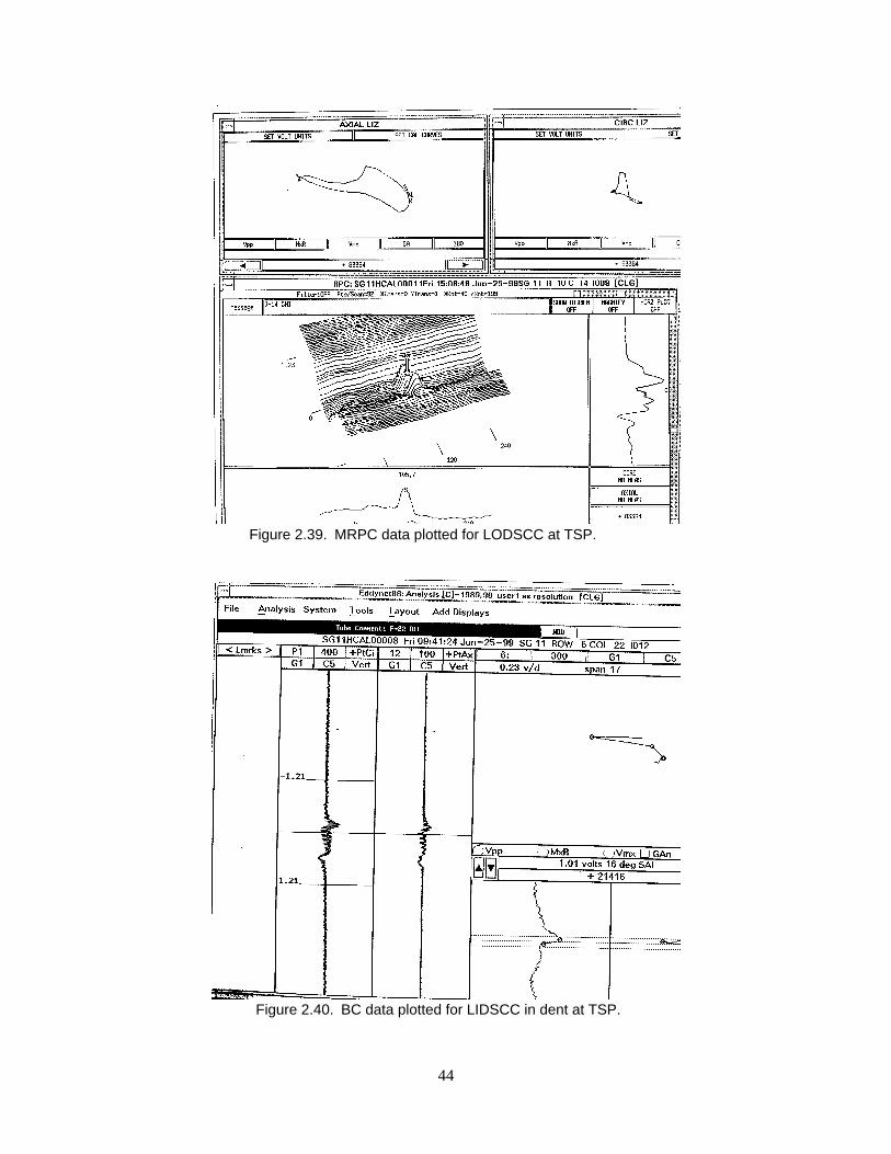
Figure 2.39. MRPC data plotted for LODSCC at TSP.

Figure 2.40. BC data plotted for LIDSCC in dent at TSP.

44

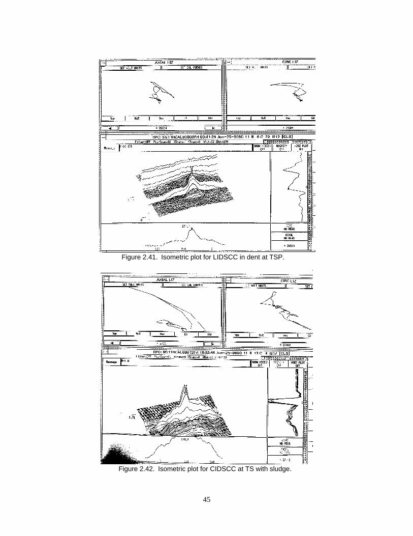
Figure 2.41. Isometric plot for LIDSCC in dent at TSP.

Figure 2.42. Isometric plot for CIDSCC at TS with sludge.

45

Figure 2.43. RPC data plotted for IGA at TSP.

2.4.2 Tolerance for Errors in Location

The location error allowed for calls made from bobbin coil data is 25 mm (1 in) from either end of the flaw along the tube axis. This allowed error equates to 30 data points for bobbin coil data. For MRPC data, the error allowed in the axial direction is also 25 mm (1 in) from the ends of the flaw along the tube axis. This allowed error equates to 3000 data points for the MRPC data.

2.4.3 Handling of False Calls

Analysts’ reports were used to determine the false call rate. The rate was determined from a review of randomly selected flaw–free test sections in the mock–up and the number of “I” codes called in those test sections. An “I” code call (NQI, DTI, DNI) signifies a flaw indication in the section, even though no flaw was actually present. In total, 522 test sections were analyzed. No known stress corrosion cracks were in any of the test sections. With 11 teams, there were 5742 chances to make a false call. The result was 6% for the tube–sheet level using MRPC data, 1.7% for the TSP with BC data, and 0.1% for the free–span with BC data. These rates are low enough to avoid any consideration of penalizing the analysts for false calls. The false call rates for the TSP and free–span would be expected to be lower than those in field inspections because of the lower noise levels in the mock–up. Because the noise levels are more comparable, the false call rate for the tube-sheet would be expected to be more comparable to that in the field. Since higher false call rates would lead to higher POD curves (TSP and free–span), the results presented in this report could be considered conservative from that stand point, although the overall effect of the lower noise on the POD is probably non-conservative because of the higher likelihood of a false negative associated with higher noise levels. However, even doubling the false call rate would have no discernible effect on the POD curves presented in this report.

46

2.4.4 Procedures for Determining POD

Data from the eleven teams participating in the RR exercise were first handled by using the EPRI “Shell” program, which had been loaded into an ANL computer. The optical disks used by the analysts contained the analysts’ reports and were read by the “Shell” Program. The program sorted the data. Calls from primary, secondary, and resolution analysts were compared to the results of expert opinion. Note that the comparison to expert opinion is not the result sought because expert opinion does not always provide the true state of the flaws. The reference state of the flaws was provided by the ANL flaw characterization algorithm, which uses a multiparameter approach to analyzing the EC data taken at multiple frequencies. All POD curves use the depth estimates determined by analyzing the EC data with the multiparameter algorithm. Three reports were analyzed for each team for each of the three parts of the RR: the bobbin coil data, the MRPC tube-sheet data, and the MRPC special–interest (spin call) data. The “Shell” program sorted the data by degradation and, for LODSCC at the tube support plate, by voltage. The principal advantage of using the “Shell” program is the ability to transfer the analysts’ reports into an Excel file, which can then be used to carry out the statistical analysis. Table 2.6 gives the number of teams analyzing the three data disks. One team was not able to complete the Special Interest MRPC disk. Table 2.7 summarizes the information provided by the EPRI “Shell” program.

Indication tables are generated for both bobbin coil and MRPC data and compared with the Flaw Indication Table, which contains all the information needed to estimate POD.

Tables 2.8 and 2.9 show simulated inputs to the Flaw Table and the Flaw Indication Table for a bobbin coil inspection. Table 2.8 shows input for a flaw in row A, column 7, at TSP level D, where the maximum BC voltage is at data point 1865 (as noted in the column “Flaw ID”). The flaw is a longitudinal ID with a BC voltage of 2.04 V and phase angle of 25 degrees. The flaw begins at data point 1839 and ends at 1873. About 3600 data points are stored for each tube examined with the bobbin coil (nine test sections). Table 2.8 shows the estimated depth to be 40% TW. This depth is determined by application of the ANL multiparameter algorithm to MRPC data for the flaw. An “I” code triggers an inspection with an MRPC. The reference–state three–letter code is SAI, single axial indication. A second example is also provided in Table 2.8. The second flaw, a longitudinal ODSCC, is at row M, column 14, and free–span level F. The result for the bobbin coil inspection is shown in Table 2.9. An indication was found in row A, column 7, at data point 1855, close to the correct flaw location. The ID/OD call is correct, and an “I” code is also called, although in this case it is DTI (distorted TSP indication). The DTI call also requires MRPC data to be acquired. The second indication would also be graded as a correct call.

Table 2.6. Number of round–robin analyst reports for the three data sets from the first eleven participating teams.

Mock–up Data Set

Number of Primary Analyst

Reports to Date

Number of Secondary

Analyst Reports to

Date

Number of Resolution

Analyst Reports to

Date Bobbin Coil (All Tubes) 11 11 11 MRPC (All Tube–Sheet Test Sections)

11 11 11

MRPC (All Special Interest, i.e., Spin Calls)

10 10 10

47

Table 2.7. Information provided by the EPRI “Shell” program using results from round–robin analysts’ reports.**

Flaw Type 2 3 4 5 6 7 8 9 10 11 12 13 14 26 27 28 Total 31 32 Total 33 34 Total

No. of Expert

Opinion Calls

* * * * * * * * * * * * * * * * * * * * * * *

No. Analyst

Calls

* * * * * * * * * * * * * * * * * * * * * * *

RMSE Volts * * * * * * *

No. of

Overcalls

* * * * * * * * * * * * * * * * * * * * * * *

*Data generated. **Note that analysts’ reports are compared to expert opinion, not to true state of the mock–up.

2 TSP/BC/ODSCC 0.25–0.49 v. 3 TSP/BC/ODSCC 0.50–0.74 v. 4 TSP/BC/ODSCC 0.75–0.99 v. 5 TSP/BC/ODSCC 1.00–.1.49 v. 6 TSP/BC/ODSCC 1.50–2.99 v. 7 TSP/BC/ODSCC > 3.00 v. 8 TSP/BC/PWSCC–Dent < 2.0 v. 9 BC/ODSCC/Free–span 10 BC/PWSCC–Ding/Free–span 11 TSP/BC/Wear/Free–span

12 TSP/BC/IGA/Free–span 13 BC/ODSCC/Sludge Pile 14 Expansion/BC/PWSCC 26 BC/ All Dents 27 BC/Other 28 TSP/BC/Thinning–Wastage/Free–span 31 +Point/PWSCC 32 +Point/ODSCC 33 +Point/Expansion/PWSCC 34 +Point/Expansion/ODSCC

Table 2.8. Simulated input to flaw table for bobbin coil inspection.

Flaw ID

Flaw

BC

Volts

BC Phase

ID/OD

Beg. Pt.

End Pt.

Depth (% TW)

Expert BC Call

True State Call

A07D1865

LID 2.04 25 ID 1839 1873 40 NQI SAI

M14F3177

LOD 2.61 70 OD 3157 3192 90 NQI SAI

Table 2.9. Simulated bobbin coil input to flaw indication table.

Indication BC Volts BC Phase ID/OD Depth Est. Call AO7 1855 2.14 29 ID 50 DTI M14 3157 2.68 60 OD 80 NQI

2.4.4.1 Converting Site–Specific Performance Demonstration (SSPD) Results to Text Files and Excel Files

The Eddynet software provides a series of files that contain the reports of results from each analyst who participated in the RR. These data are saved under an Eddynet environment and are identified by extensions that refer to primary, secondary, and resolution analysts’ reports. These files are then read by

48

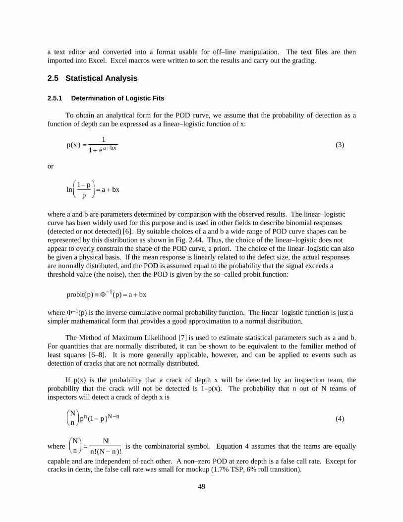
a text editor and converted into a format usable for off–line manipulation. The text files are then imported into Excel. Excel macros were written to sort the results and carry out the grading.

2.5 Statistical Analysis

2.5.1 Determination of Logistic Fits

To obtain an analytical form for the POD curve, we assume that the probability of detection as a function of depth can be expressed as a linear–logistic function of x:

p(x ) 1

1 eabx (3)

or

ln

1 p

p

a bx

where a and b are parameters determined by comparison with the observed results. The linear–logistic curve has been widely used for this purpose and is used in other fields to describe binomial responses (detected or not detected) [6]. By suitable choices of a and b a wide range of POD curve shapes can be represented by this distribution as shown in Fig. 2.44. Thus, the choice of the linear–logistic does not appear to overly constrain the shape of the POD curve, a priori. The choice of the linear–logistic can also be given a physical basis. If the mean response is linearly related to the defect size, the actual responses are normally distributed, and the POD is assumed equal to the probability that the signal exceeds a threshold value (the noise), then the POD is given by the so–called probit function:

probit(p) 1(p) a bx

where –1(p) is the inverse cumulative normal probability function. The linear–logistic function is just a simpler mathematical form that provides a good approximation to a normal distribution.

The Method of Maximum Likelihood [7] is used to estimate statistical parameters such as a and b. For quantities that are normally distributed, it can be shown to be equivalent to the familiar method of least squares [6–8]. It is more generally applicable, however, and can be applied to events such as detection of cracks that are not normally distributed.

If p(x) is the probability that a crack of depth x will be detected by an inspection team, the probability that the crack will not be detected is 1–p(x). The probability that n out of N teams of inspectors will detect a crack of depth x is

Nn

pn (1 p )N n (4)

where Nn

N!

n!(N n )! is the combinatorial symbol. Equation 4 assumes that the teams are equally

capable and are independent of each other. A non–zero POD at zero depth is a false call rate. Except for cracks in dents, the false call rate was small for mockup (1.7% TSP, 6% roll transition).

49

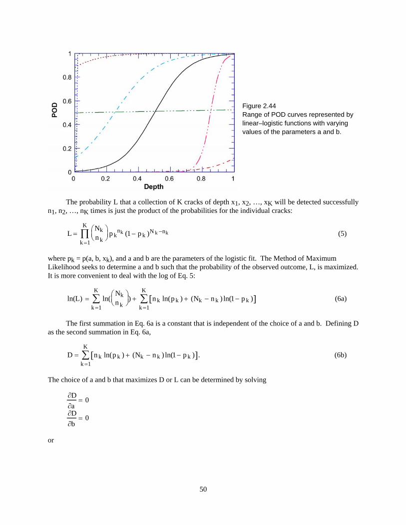
Figure 2.44 Range of POD curves represented by linear–logistic functions with varying values of the parameters a and b.

The probability L that a collection of K cracks of depth x1, x2, …, xK will be detected successfully n1, n2, …, nK times is just the product of the probabilities for the individual cracks:

L Nkn k

p knk (1 p k )N k nk

k 1

K

(5)

where pk = p(a, b, xk), and a and b are the parameters of the logistic fit. The Method of Maximum Likelihood seeks to determine a and b such that the probability of the observed outcome, L, is maximized. It is more convenient to deal with the log of Eq. 5:

ln(L) ln(Nkn k

k 1

K

) n k ln(p k ) (Nk n k ) ln(1 p k ) k 1

K

(6a)

The first summation in Eq. 6a is a constant that is independent of the choice of a and b. Defining D as the second summation in Eq. 6a,

D n k ln(p k ) (Nk n k ) ln(1 p k ) k 1

K

. (6b)

The choice of a and b that maximizes D or L can be determined by solving

D

a 0

D

b 0

or

50

n k Nk p k

p k (1 p k )p k

ak 1

K

0

n k Nk p kp k (1 p k )

p kb

k 1

K

0

(7)

Differentiating Eq. 3, we find that

p k

a p k (1 p k )

p k

b p k (1 p k )x k

(8)

Using Eqs. 8, Eqs. 7 reduce to

(n k Nk p k ) 0k 1

K

(n k Nk p k )x k 0k 1

K

(9)

Equations 9a and 9b are a pair of simultaneous nonlinear equations for a and b. For computation, it is generally more convenient to determine a and b by algorithms that directly maximize D rather than attempt to solve these equations. Excel spreadsheets were developed for this purpose and benchmarked against the commercial statistical software package STATA.

2.5.2 Uncertainties in the POD Curves

Equation 9 can be solved for a and b. These values depend on the round–robin results, i.e., on n1, n2, etc. If the round–robin was repeated with a different set of teams or a different set of cracks, different values would be obtained for a and b, i.e., there will be distributions for a and b rather than fixed values. Similarly, the actual depths of the cracks, xk, are not known exactly, instead we have a measured value ˆ x k x k k , where k is the error in the measured value of xk. The errors will be random variables.

The distributions for a and b can be characterized by mean values and variances. The mean values can be found by solving Eq. 9, although it is generally easier to obtain a and b by direct maximization of D (Eq. 6b). However, Eq. 9 involves the unknown quantities xk, where, in reality, only the measured values, ˆ x k , are known. If we denote the solution of the approximate equations,

(nk Nk ˆ p k ) 0k1

K

(nk Nk ˆ p k ) ˆ x k 0k1

K

(10)

which involve only the measured values ˆ x k as and ˆ ˆ a b , then the shift or bias in the mean values due to the errors in the measured depths ˆ x k , a and b, can be determined by expanding Eq. 9 in terms of k, a, and b. Thus

51

pk ˆ p k ˆ p ka

a ˆ p kb

bˆ p kx k

k 2ˆ p kx k

2 k2 O(a2,b2,k

3 ) (11)

The derivatives with respect to a and b are given by Eq. 8. The other derivatives are

ˆ p kx k

ˆ p k (1 ˆ p k ) ˆ b

2 ˆ p kx k

2 ˆ p kx k

(1 ˆ p k ) ˆ b ˆ p k ˆ p kx k

ˆ b

ˆ p k (1 3ˆ p k 2 ˆ p k3) ˆ b 2

(12)

If the set of trials is repeated m times, the values of a, b, and k would be different for each trial. If we average over the trials, the average value of k goes to zero, and the average values of a and b depend only on the average values of k

2 i.e., the variance which is known from NDE studies of sizing errors. Substituting from Eq. 11 into Eq. 9, using Eqs. 10, and retaining only terms O(k

2 , one can obtain equations for the average values of a and b. The final equations for the average values of a and b are

Nk ˆ p kk1

K

(1 ˆ p k)

a Nk ˆ x k ˆ p k

k1

K

(1 ˆ p k )

b Nk (ˆ p k 2ˆ p k

2 )k 1

K

(1 ˆ p k ) ˆ b 2

x k2

Nk ˆ x k ˆ p kk1

K

(1 ˆ p k)

a Nk ˆ x k

2 ˆ p kk1

K

(1 ˆ p k )

b Nkx k ˆ p k (1 2ˆ p k )

k 1

K

(1 ˆ p k ) ˆ b 2 Nk ˆ p k(1 ˆ p k )ˆ b

xk

2

(13)

where is the estimated variance of the errors in the measured depths. The variance can be

determined from comparisons of the NDE and destructive data. It will vary with the depth of the crack.

x k2 x k

2

Equations 10 and 13 give estimates of the mean values of a and b. Note that variances in dependent variables like a and b are related to the variances of the independent variables nk and xk through the propagation of error equations:

a2 nk

2 an k

2

x k2 a

x k

2

k 1

K

b2 nk

2 b

n k

2

x k2 b

x k

2

k 1

K

ab2 nk

2 an k

bn j

x k

2 ax k

bx j

k 1

K

(14)

The variance for a binomial process is nk2

52

nk2 Nk p k (1 p k )

The array is generally referred to as the covariance matrix C. a

2 ab2

ab2 b

2

The derivatives

an k

,a

xk,b

n k, and

b

xkcan be obtained from Eq. 9. Differentiating Eq. 9 with

respect to nj gives

1 Nkp k

n jk 1

K

0

x j Nk x kp kn jk 1

K

0

(15)

Differentiating Eq. 9 with respect to xj gives

Nkp k

x jk 1

K

0

n j Njp j Nk x kp kx jk 1

K

0

(16)

The partial derivatives of pk can be expressed in terms of the derivatives of a and b:

pkn j

pka

a

n jp kb

bn j

(a )

p k (1 p k )a

n j p k (1 p k ) x k

b

n j(b)

pkx j

pkxk

x k

x jp ka

a

x jp kb

b

x j(c )

p k 1 p k bkj pk (1 pk )a

x j pk (1 pk ) x k

b

x j(d )

(17)

Substituting Eq. 17 into Eqs. 15 gives

0an j

1bn j

1

1an j

2bn j

x j

(18)

where

53

0 Nk p k (1 p k )k 1

K

1 Nk p k (1 p k )k 1

K

x k

2 Nk p k (1 p k )k 1

K

x k2

(19)

Equation 18 is easily solved for the partial derivatives of a and b with respect to nj:

bn j

x j

10

12

0 2

an j

10

10

bn j

(20)

Similar expressions can be obtained for the partial derivatives of a and b with respect to xj.

Defining

(x ) ln1 p

p

a bx (21)

the variance of j corresponding to the jth crack is

j

2 a2

j

a

2

b2

j

b

2

2ab2

j

a

j

b

a2 x j

2 b2 2 x jab

2

(22)

The confidence limits for pj can be expressed in terms of j:

p j 1

1 ej Z j

(23)

where Z is a constant that depends on the confidence level desired.

2.5.3 Significance of Difference between Two POD Curves

There are a several ways to test whether two POD curves are the same. The test described below is the easiest because it only requires the logistic regression results. A logistic regression is run on two sets of data. Each regression fit has as a result a set of parameter estimates u = (a,b) and an associated covariance matrix C. The two data sets are designated by letters and and the two regression fits are described by

54

p,i = logistic(a,1 +b,2 x,i ) (24)

p,i = logistic(a,1 +b,2 x,i ) (25)

The regression fits produce the estimates u and u, along with the covariance matrices C and C. To test whether u = u , one forms a chi–squared statistic:

2 = (u – u)T [C + C]–1 (u – u) (26)

and compares 2 to a critical value obtained from a chi–squared table. The degree of freedom associated with the critical value equals the number of model parameters; in this case, two. The two sets of parameters are equal when 2 is less than the critical value. For example, to conduct the test at a 10% level of significance, the critical value would be 4.61.

A chi–squared table can also be used to assign a p–value to the statistic 2. When performing this test, a less stringent level of significance than typical can be used, such as 10% or 20% instead of the typical 5%. This approach has been used to determine if POD curves by different teams using the same data are different by chance or if the difference is significant.

2.5.4 Alternate Forms of the POD Curves

Although the linear–logistic form is widely used to describe POD curves, other forms of the analysis of binomial data need to be considered. If the linear–logistic equation is written in the form

ln

p

1 p

a bx , (27)

then other potential forms include the log–logistic:

ln

p

1 p

a bln(x) (28)

and the linear–log–log:

ln(ln(p)) = a + bx. (29)

Like the linear–logistic, the choice of the log–logistic can be justified in terms of a physical argument. If the mean response is exponentially related to the defect size, the actual response is log–normally distributed, and the POD is assumed equal to the probability that the signal exceeds a threshold value (the noise), then the POD is given the log–normal equivalent of the probit function, which can be approximated by the log–logistic. An application of these models to detection data from the mockup is shown in Fig. 2.45.

55

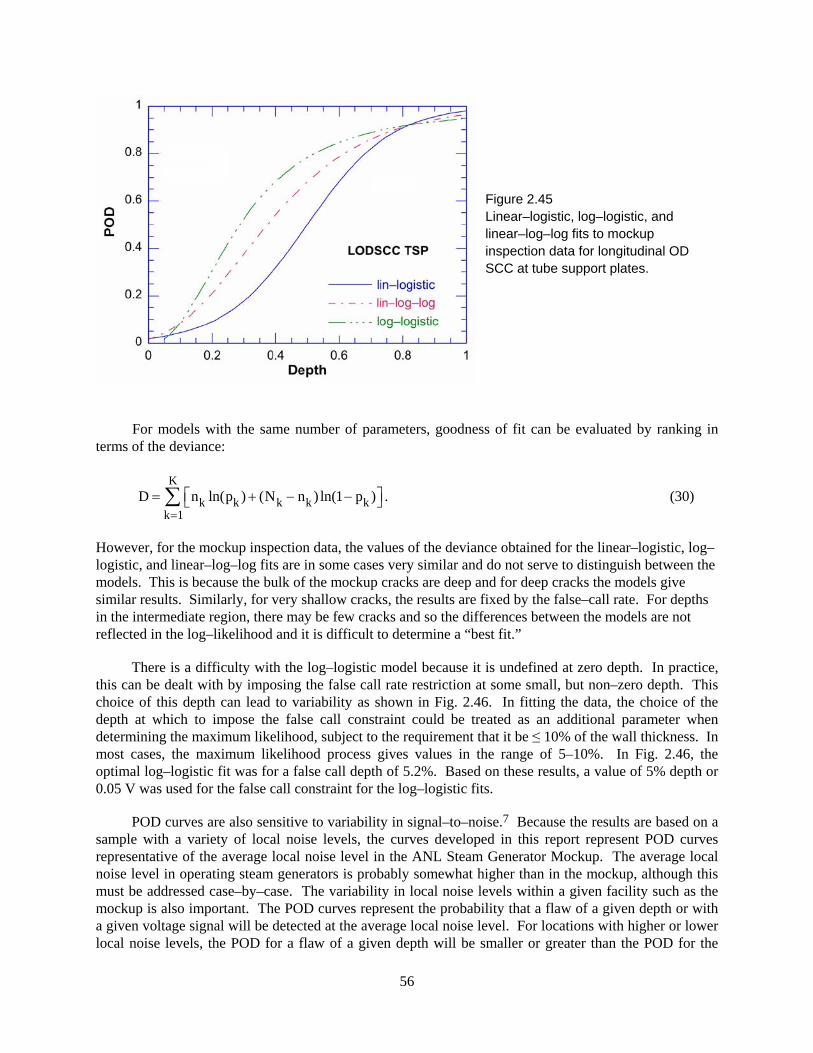
Figure 2.45 Linear–logistic, log–logistic, and linear–log–log fits to mockup inspection data for longitudinal OD SCC at tube support plates.

For models with the same number of parameters, goodness of fit can be evaluated by ranking in terms of the deviance:

. (30)

D nk ln(pk ) (Nk nk ) ln(1 pk ) k1

K

However, for the mockup inspection data, the values of the deviance obtained for the linear–logistic, log–logistic, and linear–log–log fits are in some cases very similar and do not serve to distinguish between the models. This is because the bulk of the mockup cracks are deep and for deep cracks the models give similar results. Similarly, for very shallow cracks, the results are fixed by the false–call rate. For depths in the intermediate region, there may be few cracks and so the differences between the models are not reflected in the log–likelihood and it is difficult to determine a “best fit.”

There is a difficulty with the log–logistic model because it is undefined at zero depth. In practice, this can be dealt with by imposing the false call rate restriction at some small, but non–zero depth. This choice of this depth can lead to variability as shown in Fig. 2.46. In fitting the data, the choice of the depth at which to impose the false call constraint could be treated as an additional parameter when determining the maximum likelihood, subject to the requirement that it be ≤ 10% of the wall thickness. In most cases, the maximum likelihood process gives values in the range of 5–10%. In Fig. 2.46, the optimal log–logistic fit was for a false call depth of 5.2%. Based on these results, a value of 5% depth or 0.05 V was used for the false call constraint for the log–logistic fits.

POD curves are also sensitive to variability in signal–to–noise.7 Because the results are based on a sample with a variety of local noise levels, the curves developed in this report represent POD curves representative of the average local noise level in the ANL Steam Generator Mockup. The average local noise level in operating steam generators is probably somewhat higher than in the mockup, although this must be addressed case–by–case. The variability in local noise levels within a given facility such as the mockup is also important. The POD curves represent the probability that a flaw of a given depth or with a given voltage signal will be detected at the average local noise level. For locations with higher or lower local noise levels, the POD for a flaw of a given depth will be smaller or greater than the POD for the

56

Figure 2.46. Effect of the choice of depth (identified as % TW) at which to impose the false call constraint on log–logistic fits for the POD curve for LODSCC at the TSP. The choice of the 5% TW depth gives the optimum fit.

average level. Reference 7 presents estimates of the potential effect of local noise for the mockup and for the potential effect of differences between the average local noise level in the mockup and operating steam generators.

2.6 Results of Round–Robin Analysis

2.6.1 POD Curve Fits

2.6.1.1 Bobbin Coil Results

The reference table in Appendix B shows the important characteristic parameters of the axial flaws: max depth, mp, and average depth. The flaw characterization parameters were determined from the profiles generated by the multiparameter algorithm. The results reported here are derived from the bobbin coil reports of resolution analysts from the eleven RR teams. Analysts are given credit for calling a flaw if their reported flaw location is within 25 mm (1 in) of the ends of the flaw. The analyst’s estimate of depth was not a factor in calculating POD.

The bobbin coil voltages reported for LODSCC at tube support plates by teams analyzing the mock–up data have been statistically examined. In most cases, the differences in the voltage reported by the different teams were small. For each LODSCC, an average BC voltage and a corresponding standard deviation were computed. The cumulative distribution of the normalized standard deviations (i.e., the standard deviation divided by the corresponding value of the average voltage) can be fit well by a Weibull distribution (the RMS difference between the observed distribution and the Weibull fit is < 0.03). The fitted distribution is shown in Fig. 2.47. For almost 90% of the indications, the normalized standard deviation in the reported voltages is < 0.15. This result is consistent with NRC Generic Letter 95–05, which assumes that a 15% cutoff for the voltage–response variability distribution is acceptable. The indications with larger variations are not associated with particularly high or low voltages (i.e., approximately half the signals with standard deviations > 0.1 have voltages > 2 V), but are associated with the complexity of the signal and the difficulty in identifying the peak voltage.

Figure 2.48 shows maximum likelihood fits for the POD with LODSCC at the TSP as a function of maximum depth as determined from the multiparameter algorithm. These are composite results based on

57

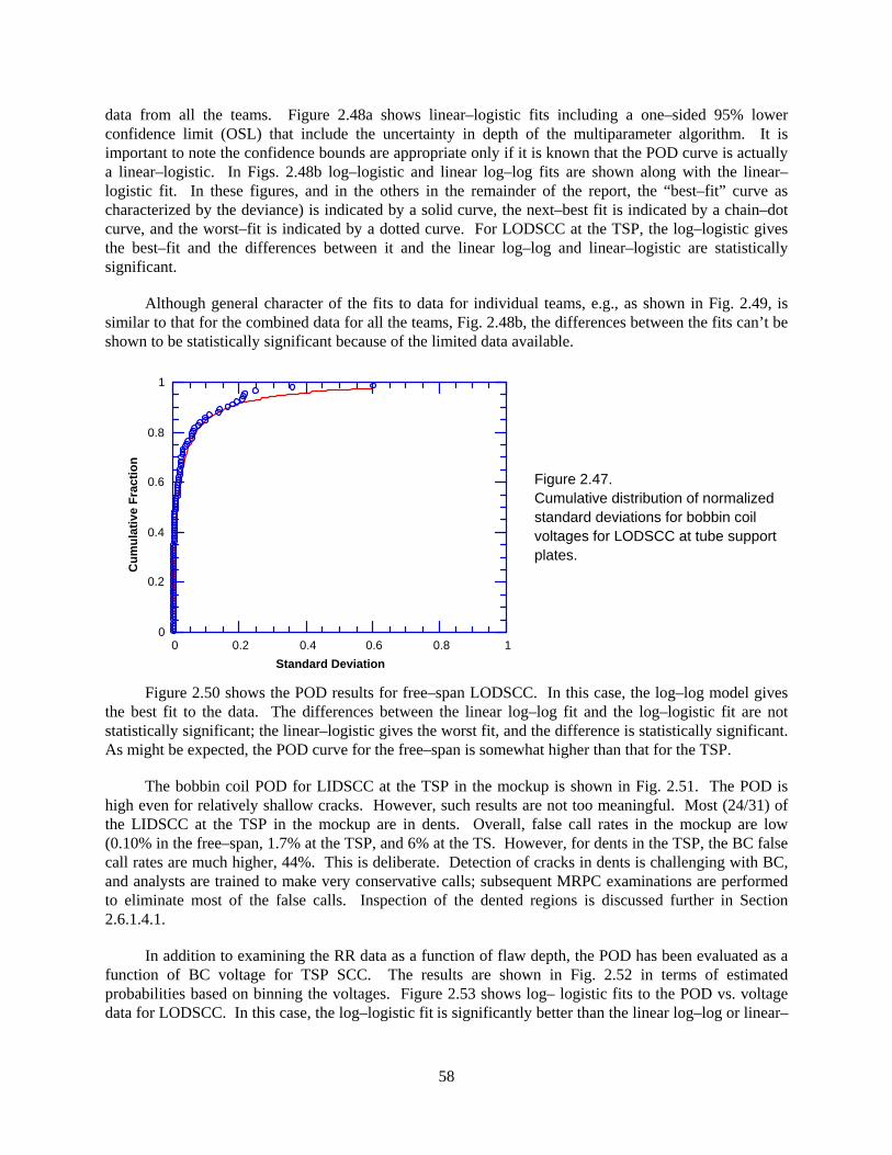
data from all the teams. Figure 2.48a shows linear–logistic fits including a one–sided 95% lower confidence limit (OSL) that include the uncertainty in depth of the multiparameter algorithm. It is important to note the confidence bounds are appropriate only if it is known that the POD curve is actually a linear–logistic. In Figs. 2.48b log–logistic and linear log–log fits are shown along with the linear–logistic fit. In these figures, and in the others in the remainder of the report, the “best–fit” curve as characterized by the deviance) is indicated by a solid curve, the next–best fit is indicated by a chain–dot curve, and the worst–fit is indicated by a dotted curve. For LODSCC at the TSP, the log–logistic gives the best–fit and the differences between it and the linear log–log and linear–logistic are statistically significant.

Although general character of the fits to data for individual teams, e.g., as shown in Fig. 2.49, is similar to that for the combined data for all the teams, Fig. 2.48b, the differences between the fits can’t be shown to be statistically significant because of the limited data available.

0

0.2

0.4

0.6

0.8

1

0 0.2 0.4 0.6 0.8 1

Cu

mu

lati

ve F

ract

ion

Standard Deviation

Figure 2.47. Cumulative distribution of normalized standard deviations for bobbin coil voltages for LODSCC at tube support plates.

Figure 2.50 shows the POD results for free–span LODSCC. In this case, the log–log model gives the best fit to the data. The differences between the linear log–log fit and the log–logistic fit are not statistically significant; the linear–logistic gives the worst fit, and the difference is statistically significant. As might be expected, the POD curve for the free–span is somewhat higher than that for the TSP.

The bobbin coil POD for LIDSCC at the TSP in the mockup is shown in Fig. 2.51. The POD is high even for relatively shallow cracks. However, such results are not too meaningful. Most (24/31) of the LIDSCC at the TSP in the mockup are in dents. Overall, false call rates in the mockup are low (0.10% in the free–span, 1.7% at the TSP, and 6% at the TS. However, for dents in the TSP, the BC false call rates are much higher, 44%. This is deliberate. Detection of cracks in dents is challenging with BC, and analysts are trained to make very conservative calls; subsequent MRPC examinations are performed to eliminate most of the false calls. Inspection of the dented regions is discussed further in Section 2.6.1.4.1.

In addition to examining the RR data as a function of flaw depth, the POD has been evaluated as a function of BC voltage for TSP SCC. The results are shown in Fig. 2.52 in terms of estimated probabilities based on binning the voltages. Figure 2.53 shows log– logistic fits to the POD vs. voltage data for LODSCC. In this case, the log–logistic fit is significantly better than the linear log–log or linear–

58

logistic fits. An industry voltage–based POD curve referred to as the POPCD curve8 is shown for comparison. The agreement between the two is reasonably good.

(a) (b) Figure 2.48. BC POD for TSP data as a function of maximum depth for LODSCC and LIDSCC using

maximum likelihood fits; (a) linear–logistic fit and the one–sided 95% confidence limit (OSL) including uncertainty in the maximum depth; (b) linear–logistic, linear log–log, and log–logistic fits for LODSCC. The solid curve in each figure is the best–fit to the data.

Figure 2.49. BC POD for TSP data as a function of maximum depth (as fraction through–wall) for LODSCC using maximum likelihood fits. The fits are to data from one team only. The circles show the raw data from which the curve is generated. Depths are determined with the multiparameter algorithm. Although the log–logistic is the best–fit, differences between the models for this team are not statistically significant.

59

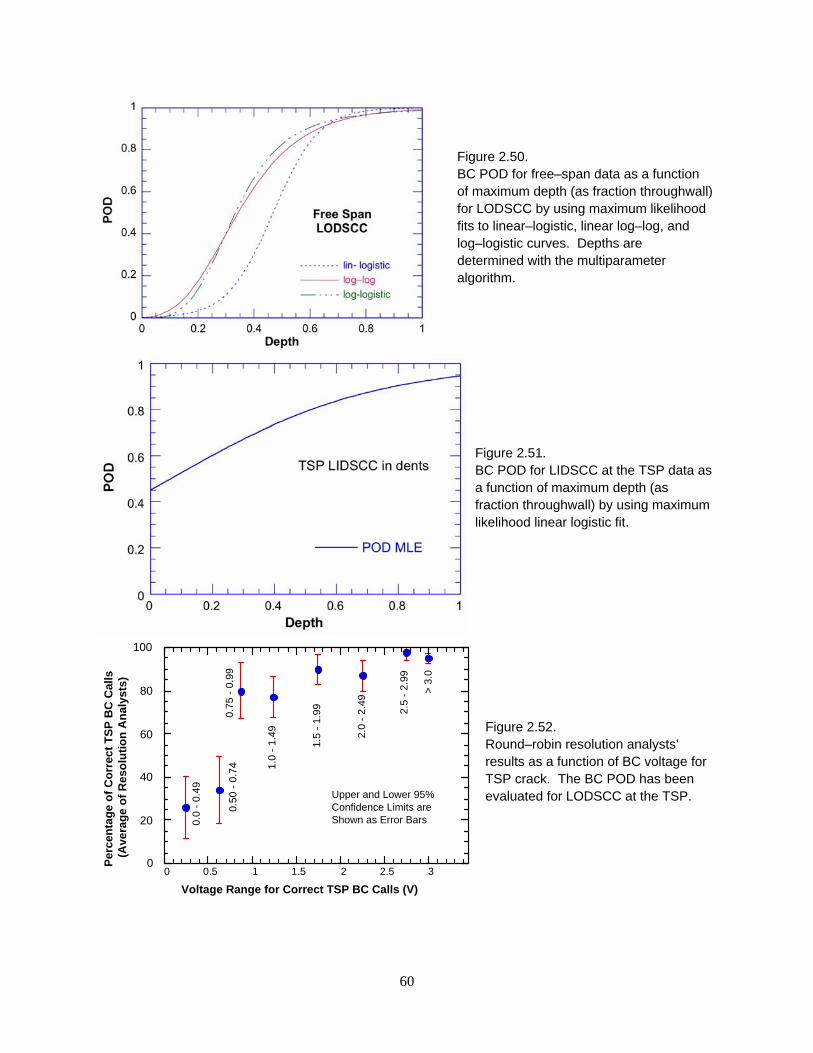
Figure 2.50. BC POD for free–span data as a function of maximum depth (as fraction throughwall) for LODSCC by using maximum likelihood fits to linear–logistic, linear log–log, and log–logistic curves. Depths are determined with the multiparameter algorithm.

Figure 2.51. BC POD for LIDSCC at the TSP data as a function of maximum depth (as fraction throughwall) by using maximum likelihood linear logistic fit.

0

20

40

60

80

100

0 0.5 1 1.5 2 2.5 3

Per

cen

tag

e o

f C

orr

ect

TS

P B

C C

alls

(Ave

rag

e o

f R

eso

luti

on

An

alys

ts)

Voltage Range for Correct TSP BC Calls (V)

0.0

- 0.

49

0.50

- 0

.74

0.75

- 0

.99

1.0

- 1.

49

> 3

.0

Upper and Lower 95%Confidence Limits areShown as Error Bars

1.5

- 1.

99

2.0

- 2.

49

2.5

- 2.

99

Figure 2.52. Round–robin resolution analysts’ results as a function of BC voltage for TSP crack. The BC POD has been evaluated for LODSCC at the TSP.

60

Figure 2.53. Log–logistic fits for BC POD as a function of voltage for LODSCC in TSP. POPCD is a voltage–based POD curve developed by industry.

The results were also analyzed by teams to determine whether strong team–to–team variations in the POD exist. All teams were given optical disks containing exactly the same data to analyze. All analysts were given the same instructions and documents related to analyzing the data. Team–to–team variations resulted from varying analyst interpretations of the same signals. The results as a function of team for free–span and TSP LODSCC combined are shown in Fig. 2.54. The performance of most of the teams clusters rather tightly, although there is a significant variation between best and worst. Figure 2.55 shows team–by–team variation for free–span LODSCC alone.

Based on the procedure discussed in Section 2.5.2, we can estimate the probability that team–to–team variations in logistic fits to data are due to chance. For FS LODSCC, the variation from best to worst (Fig. 2.55) is probably significant. The probability is < 20% that the difference is due to chance (DTC). For free–span and TSP LODSCC combined (Fig. 2.54), the variation from best to worst (DTC > 60%) is probably not significant.

61

Figure 2.56 shows the POD linear–logistic fits for LODSCC at the TSP as a function of mp. Figure 2.57 shows the fits for POD for axial SCC in free–span test sections as a function of mp. In the case of mp, the linear–logistic fits are statistically much more robust than either the log–logistic or linear log–log fits. The errors in calculating mp by using the NDE characterization of the crack geometry compared to using fractography data have been determined with the 23–tube set (Tables 2.3 and 2.4 and Fig. 2.22). Because only one value of mp per crack is obtained, fewer data are available than in the case of depth (multiple points per crack); hence, estimates of mp have greater uncertainty. In both graphs, the 95% one–sided lower confidence limit includes the error due to the use of NDE data to calculate mp, as well as the statistical uncertainties associated with finite samples. In the TSP and FS regions, the POD for cracks that would fail or leak under 3p internal pressure (corresponding to mp ≈ 2.3) is > 95%, even when accounting for depth uncertainties.

Figure 2.54. BC POD by team for free–span and TSP LODSCC combined as a function of depth. The maximum crack depth (as fraction of wall) was determined by the multiparameter algorithm. The highest solid line represents the best team, the lowest dashed line represents the worst team, and the other symbols represent the remaining teams.

0

0.2

0.4

0.6

0.8

1

0 0.2 0.4 0.6 0.8 1

PO

D

Depth

FreespanLODSCC

Figure 2.55. BC POD by team for free–span LODSCC as function of depth. The maximum crack depth (as fraction of wall) was determined by the multiparameter algorithm. The solid line represents the best team, while the symbols and dashed line represent the remaining teams.

62

0

0.2

0.4

0.6

0.8

1

1 1.5 2 2.5 3

POD95 OSL

PO

D

mp

TSP LODSCC

Figure 2.56. BC POD for TSP LODSCC as a function of mp. Curves derived by maximum likelihood fit and an estimate of the one–sided 95% confidence limit. The values of mp are derived by using depths from the multiparameter algorithm.

0

0.2

0.4

0.6

0.8

1

1 1.5 2 2.5 3

POD95 OSL

PO

D

mp

FreespanLODSCC

Figure 2.57. BC POD for free–span data for LODSCC as a function of mp. Curves derived by maximum likelihood fit and an estimate of the one–sided 95% confidence limit. The values of mp are derived by using depths from the multiparameter algorithm.

The analysis presented in this section is based on the resolution analysts’ reports. In some cases, the bobbin coil signal was difficult to analyze, and significant disagreement occurred between the calls of the resolution analyst and the primary and secondary analysts. Three examples for the TSP are presented here. The first is for a 39% TW LIDSCC, the second is for a 67% TW LODSCC, and the third is for a very short 99% TW LODSCC. Table 2.10 shows that while for 13 out of the 33 cases all analysts were in agreement with respect to making I–code calls with the bobbin coil data; for the other 20 cases, there was disagreement. In 13 of the 20 cases, the resolution analysts incorrectly dismissed a correct call by the primary and/or secondary analyst. In four cases, the resolution analysts made a correct call while the primary and/or secondary analysts did not. In three cases, all analysts made incorrect calls. These examples show significant team–to–team variations for difficult–to–analyze signals and suggest that limiting the impact that the resolution analysts have in making the final call for these types of SCC might be prudent.

63

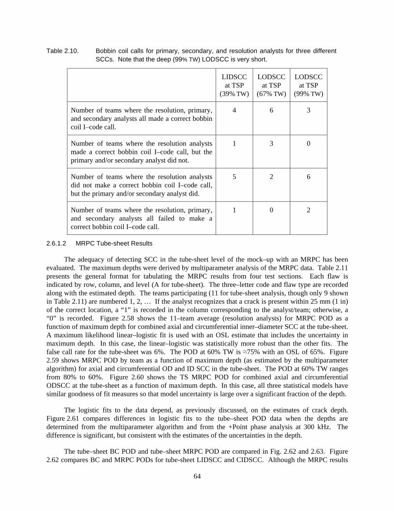
Table 2.10. Bobbin coil calls for primary, secondary, and resolution analysts for three different SCCs. Note that the deep (99% TW) LODSCC is very short.

LIDSCC at TSP

(39% TW)

LODSCC at TSP

(67% TW)

LODSCC at TSP

(99% TW)

Number of teams where the resolution, primary, and secondary analysts all made a correct bobbin coil I–code call.

4 6 3

Number of teams where the resolution analysts made a correct bobbin coil I–code call, but the primary and/or secondary analyst did not.

1 3 0

Number of teams where the resolution analysts did not make a correct bobbin coil I–code call, but the primary and/or secondary analyst did.

5 2 6

Number of teams where the resolution, primary, and secondary analysts all failed to make a correct bobbin coil I–code call.

1 0 2

2.6.1.2 MRPC Tube-sheet Results

The adequacy of detecting SCC in the tube-sheet level of the mock–up with an MRPC has been evaluated. The maximum depths were derived by multiparameter analysis of the MRPC data. Table 2.11 presents the general format for tabulating the MRPC results from four test sections. Each flaw is indicated by row, column, and level (A for tube-sheet). The three–letter code and flaw type are recorded along with the estimated depth. The teams participating (11 for tube-sheet analysis, though only 9 shown in Table 2.11) are numbered 1, 2, … If the analyst recognizes that a crack is present within 25 mm (1 in) of the correct location, a “1” is recorded in the column corresponding to the analyst/team; otherwise, a “0” is recorded. Figure 2.58 shows the 11–team average (resolution analysts) for MRPC POD as a function of maximum depth for combined axial and circumferential inner–diameter SCC at the tube-sheet. A maximum likelihood linear–logistic fit is used with an OSL estimate that includes the uncertainty in maximum depth. In this case, the linear–logistic was statistically more robust than the other fits. The false call rate for the tube-sheet was 6%. The POD at 60% TW is ≈75% with an OSL of 65%. Figure 2.59 shows MRPC POD by team as a function of maximum depth (as estimated by the multiparameter algorithm) for axial and circumferential OD and ID SCC in the tube-sheet. The POD at 60% TW ranges from 80% to 60%. Figure 2.60 shows the TS MRPC POD for combined axial and circumferential ODSCC at the tube-sheet as a function of maximum depth. In this case, all three statistical models have similar goodness of fit measures so that model uncertainty is large over a significant fraction of the depth.

The logistic fits to the data depend, as previously discussed, on the estimates of crack depth. Figure 2.61 compares differences in logistic fits to the tube–sheet POD data when the depths are determined from the multiparameter algorithm and from the +Point phase analysis at 300 kHz. The difference is significant, but consistent with the estimates of the uncertainties in the depth.

The tube–sheet BC POD and tube–sheet MRPC POD are compared in Fig. 2.62 and 2.63. Figure 2.62 compares BC and MRPC PODs for tube-sheet LIDSCC and CIDSCC. Although the MRPC results

64

are best fit with a linear–logistic, the linear–logistic and log–logistic fits can’t be distinguished on statistical grounds and both are shown in the figure. Figure 2.63 compares BC and MRPC POD for tube-sheet LIDSCC only. Again the linear–logistic and log–logistic fits can’t be distinguished statistically. However even considering the large uncertainties in the BC PODs, it is clear that the MRPC POD curve is substantially higher than the BC POD, especially for very deep flaws.

Table 2.11. Format for tabulating MRPC TS results (11 teams analyzed MRPC data from the tube-sheet).

Flaw ID

MRPC Location

Three– Letter Code

FlawType

Depth% TW 1 2 3 4 5 6 7 8 9

H21A 14314 MAI LOD 51 0 1 1 1 1 0 1 1 1 N18A 20550 MCI COD 85 1 1 1 1 1 1 1 1 1 N08A 20286 MAI LID 87 1 1 1 1 1 1 1 0 1 K24A 21870 MMI LOD 90 1 1 0 1 0 1 1 0 1

Figure 2.58. Tube–sheet MRPC POD as a function of maximum depth (as fraction of wall) for axial and circumferential inner–diameter SCC. Depths are determined with the multiparameter algorithm.

65

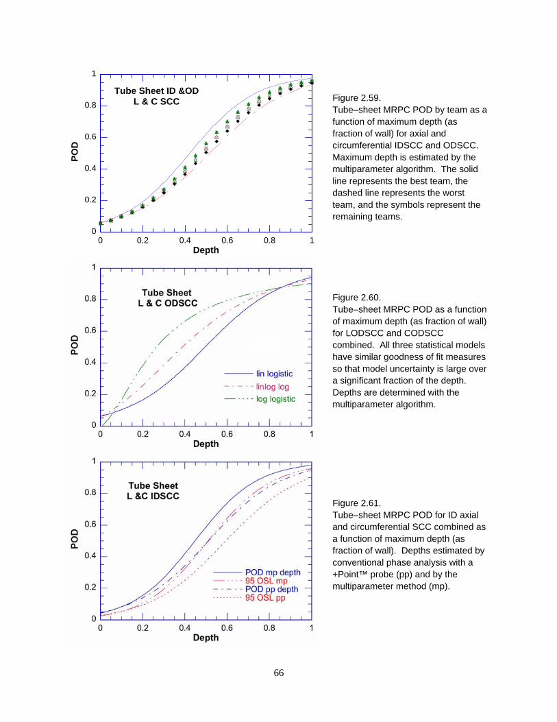
0

0.2

0.4

0.6

0.8

1

0 0.2 0.4 0.6 0.8 1

PO

D

Depth

Tube Sheet ID &ODL & C SCC

Figure 2.59. Tube–sheet MRPC POD by team as a function of maximum depth (as fraction of wall) for axial and circumferential IDSCC and ODSCC. Maximum depth is estimated by the multiparameter algorithm. The solid line represents the best team, the dashed line represents the worst team, and the symbols represent the remaining teams.

Figure 2.60. Tube–sheet MRPC POD as a function of maximum depth (as fraction of wall) for LODSCC and CODSCC combined. All three statistical models have similar goodness of fit measures so that model uncertainty is large over a significant fraction of the depth. Depths are determined with the multiparameter algorithm.

Figure 2.61. Tube–sheet MRPC POD for ID axial and circumferential SCC combined as a function of maximum depth (as fraction of wall). Depths estimated by conventional phase analysis with a +Point™ probe (pp) and by the multiparameter method (mp).

66

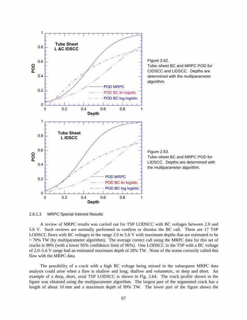
Figure 2.62. Tube–sheet BC and MRPC POD for CIDSCC and LIDSCC. Depths are determined with the multiparameter algorithm.

Figure 2.63. Tube–sheet BC and MRPC POD for LIDSCC. Depths are determined with the multiparameter algorithm.

2.6.1.3 MRPC Special Interest Results

A review of MRPC results was carried out for TSP LODSCC with BC voltages between 2.0 and 5.6 V. Such reviews are normally performed to confirm or dismiss the BC call. There are 17 TSP LODSCC flaws with BC voltages in the range 2.0 to 5.6 V with maximum depths that are estimated to be > 70% TW (by multiparameter algorithm). The average correct call using the MRPC data for this set of cracks is 98% (with a lower 95% confidence limit of 96%). One LODSCC in the TSP with a BC voltage of 2.0–5.6 V range had an estimated maximum depth of 28% TW. None of the teams correctly called this flaw with the MRPC data.

The possibility of a crack with a high BC voltage being missed in the subsequent MRPC data analysis could arise when a flaw is shallow and long, shallow and volumetric, or deep and short. An example of a deep, short, axial TSP LODSCC is shown in Fig. 2.64. The crack profile shown in the figure was obtained using the multiparameter algorithm. The largest part of the segmented crack has a length of about 10 mm and a maximum depth of 99% TW. The lower part of the figure shows the

67

projection of the crack on the axial plane. The dye penetrant image of the crack intersection with the tube OD is consistent with the isometric image generated by the multiparameter algorithm. The mp for this flaw is ≈4.5, indicating that the tube would leak at pressures well below 3p. The crack was missed by some teams analyzing MRPC data. The MRPC +Point voltage at 300 kHz was only ≈0.2 V. The reported BC voltage for this crack varied from 4.5 to 8 V.

These results illustrate that flaws detected correctly by bobbin coil inspections can subsequently be dismissed upon further examination of MRPC data, even when flaws are relatively deep. MRPC probes are very effective in characterizing defects, compared to bobbin coils, but in some cases may be less effective than bobbin coils in recognizing that a crack is present.

Figure 2.64. Depth profiles of TSP LODSCC with maximum depth of 99% TW that was missed by all teams analyzing MRPC data. The largest piece of the segmented crack has a length of about 10 mm (0.4 in). The lower part of the figure shows the crack along the test section axis.

68

2.6.1.4 Analysis of Subsets of Data

2.6.1.4.1 Dented TSP with LIDSCC

The BC and MRPC results for LIDSCC in dented TSP test sections have been analyzed as a subset of the mock–up data (using resolution analyst reports). Figure 2.65 shows the BC voltage vs. maximum LIDSCC depth as determined from the Argonne multiparameter algorithm. The voltages are large because of the dents. As expected since the amplitude is dominated by the response to the dent, the BC voltage does not correlate with maximum crack depth.

Figure 2.66 shows the results for the 11 teams using the bobbin coil data only. This graph shows the detection rate increasing with depth. The overall success in detecting an LIDSCC in a dented TSP location is somewhat less than for LIDSCC in TSP locations without dents. Nevertheless, success with a bobbin coil in detecting LIDSCC in a dent is generally high for depths greater than 40% TW. However, as noted in the previous section, the relatively high POD for LIDSCC in dents appears to be strongly influenced by the conservatism of the analysts in making such calls, which leads to a very high false call rate, 44%. Detection as a function of BC voltage is presented in Fig. 2.67. The dent signal can mask the presence of a SCC, but for the 2.5–4.5 volt range, the detection rate was generally good whether due to actual analysis of the signal or due to the conservatism of the analysts in inspecting dented regions.

Figure 2.68 shows the result for a correct call using the BC data followed by a correct call using the MRPC data for the same SCC. It is evident (Fig. 2.68) that some mock–up LIDSCCs in a dented TSP were detected by the BC data, presumably due to very conservative calls, but then incorrectly dismissed using the MRPC data. Figure 2.69 shows the results for those LIDSCCs correctly called with BC data and then dismissed with the MRPC data. Most but not all of those cases are for depths less than about 50% TW.

Figure 2.70 shows the result for a BC miss but detection with an MRPC. Some of the shallow mock–up LIDSCCs missed by the BC could be detected with the MRPC data. Figure 2.71 shows the result for LIDSCCs in a dented TSP where there was a miss with both BC and MRPC data. The double misses are mainly for shallow LIDSCCs.

As noted previously, there were numerous false calls in test sections with a dent but no SCC. Figure 2.72 shows the result for dented TSP test sections without SCC as a function of BC dent voltage. In more than half of the dented test sections without an SCC, an “I Code” was called. This is a very high false call rate and explains the apparently high BC POD for SCC in a dent. In reality, it is very difficult to detect SCC in dents with BC. However, with the MRPC data the dents without SCC were easily characterized.

Figure 2.73 summarizes the results for LIDSCCs in dented TSP test sections by showing the correct calls using MRPC data only as a function of maximum crack depth. The MRPC reports from resolution analysts were used for this graph.

2.6.1.4.2 Intergranular Attack

The round–robin results for the small number of test sections with IGA were analyzed separately from the other flawed test sections. The resolution analyst calls using bobbin coil data for the 11 teams are presented in Fig. 2.74 for IGA. The maximum depths were determined using Argonne’s multiparameter algorithm. The results suggest that for depths greater than 40% TW this type of volumetric cracking can be detected easily with a bobbin coil.

69

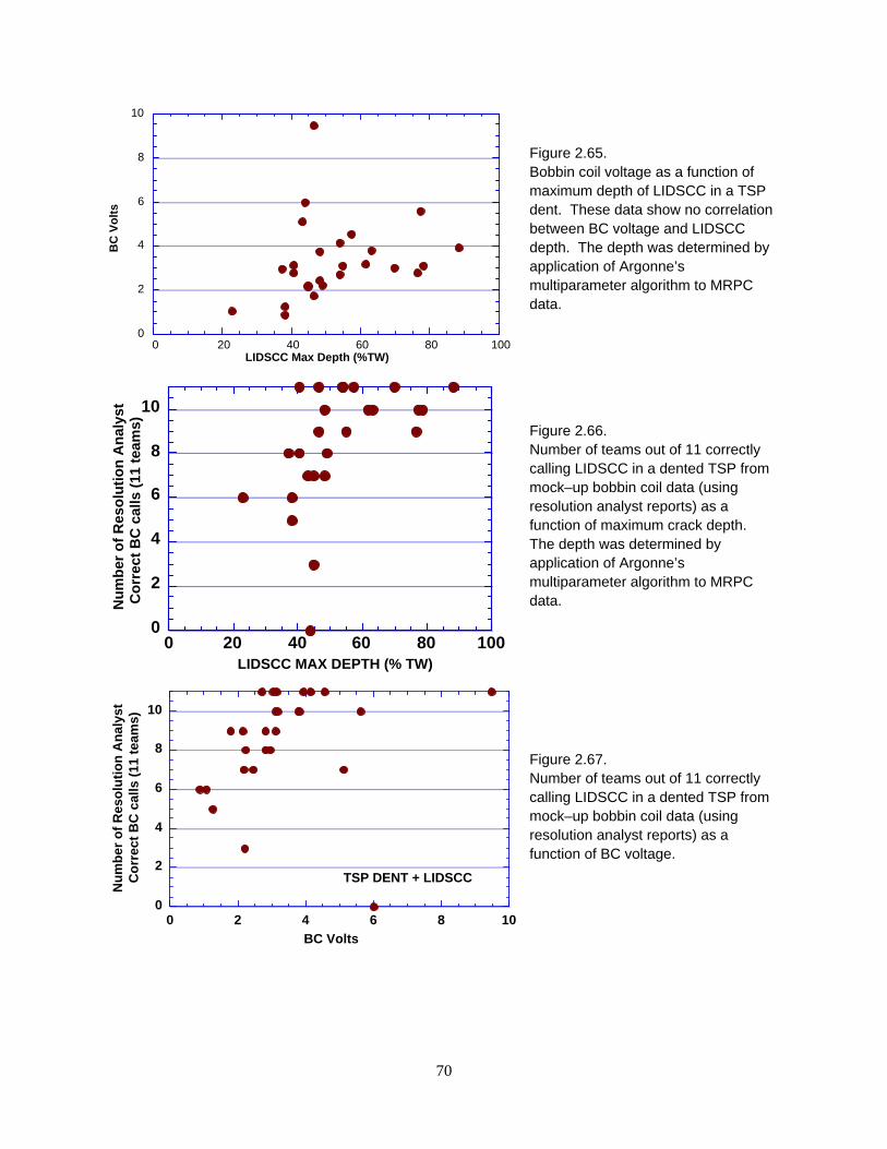
0

2

4

6

8

10

0 20 40 60 80

BC

Vo

lts

LIDSCC Max Depth (%TW)100

Figure 2.65. Bobbin coil voltage as a function of maximum depth of LIDSCC in a TSP dent. These data show no correlation between BC voltage and LIDSCC depth. The depth was determined by application of Argonne’s multiparameter algorithm to MRPC data.

0

2

4

6

8

10

0 20 40 60 80 100

Nu

mb

er o

f R

eso

luti

on

An

alys

tC

orr

ect

BC

cal

ls (

11 t

eam

s)

LIDSCC MAX DEPTH (% TW)

Figure 2.66. Number of teams out of 11 correctly calling LIDSCC in a dented TSP from mock–up bobbin coil data (using resolution analyst reports) as a function of maximum crack depth. The depth was determined by application of Argonne’s multiparameter algorithm to MRPC data.

0

2

4

6

8

10

0 2 4 6 8

TSP DENT + LIDSCC

Nu

mb

er o

f R

eso

luti

on

An

alys

tC

orr

ect

BC

cal

ls (

11 t

eam

s)

BC Volts

10

Figure 2.67. Number of teams out of 11 correctly calling LIDSCC in a dented TSP from mock–up bobbin coil data (using resolution analyst reports) as a function of BC voltage.

70

0

2

4

6

8

10

0 20 40 60 80 1

Nu

mb

er o

f C

orr

ect

BC

Cal

ls F

oll

ow

ed

by

Co

rrec

t M

RP

C C

all

(10

Tea

ms)

LIDSCC Max Depth (% TW)

00

Figure 2.68. Number of teams out of 10 correctly calling an LIDSCC in a dented TSP from mock–up bobbin coil data followed by a correct call for that crack using MRPC data (from resolution analyst reports) as a function of maximum crack depth. The depth was determined by application of Argonne’s multiparameter algorithm to MRPC data.

0

2

4

6

8

10

0 20 40 60 80 1

Nu

mb

er o

f C

orr

ect

BC

Cal

lsD

ism

isse

d b

y M

RP

C D

ata

(10

Tea

ms)


00

Figure 2.69. Number of teams out of 10 correctly calling an LIDSCC in a dented TSP from bobbin coil data followed by dismissing that crack using MRPC data (from resolution analyst reports) as a function of maximum crack depth. The depth was determined by application of Argonne’s multiparameter algorithm to MRPC data.

0

2

4

6

8

10

0 20 40 60 80 1

TSP DENT + LIDSCC

Nu

mb

er o

f C

orr

ect

MR

PC

Cal

lsW

ith

Mis

sed

BC

Ca

ll (1

0 T

eam

s)


00

Figure 2.70. Number of teams out of 10 missing an LIDSCC in a dented TSP from bobbin coil data followed by a correct call using MRPC data (from resolution analyst reports) as a function of maximum crack depth. The depth was determined by application of Argonne’s multiparameter algorithm to MRPC data.

71

0

2

4

6

8

10

0 20 40 60 80 100

TSP DENT + LIDSCCNu

mb

er

of

Re

so

luti

on

An

aly

sts

Mis

se

s b

y b

oth

MR

PC

an

d B

C (

10

Te

am

s)


Figure 2.71. Number of teams out of 10 missing an LIDSCC in a dented TSP with both bobbin coil and MRPC data (from resolution analyst reports) as a function of maximum crack depth. The depth was determined by application of the multiparameter algorithm to MRPC data.

0

0.4

0.8

1.2

1.6

2

2.4

2.8

3.2

0 2 4 6 8 10

TSP DENT without LIDSCC

BC

Vo

lts

NUMBER OF FALSE CALLS (Resolution Analysts for11 teams)

Figure 2.72. Number of false calls in dented TSP test sections as a function of BC voltage (0.1–V window).

Figure 2.73. Number of teams correctly calling an LIDSCC in a dented TSP using MRPC data

(from resolution analyst reports) as a function of maximum crack depth. The depth was determined by application of Argonne’s multiparameter algorithm to MRPC data.

72

Figure 2.74. Number of teams out of 11 correctly calling IGA from bobbin coil data (using

resolution analyst reports) as a function of maximum flaw depth. The depth was determined by application of Argonne’s multiparameter algorithm to MRPC data.

2.6.1.4.3 EDM Notches and Laser Cut Slots

Figure 2.75 shows the POD results for EDM notches and laser cut slots. The very high detection rate for all but an approximately 40% TW deep notch suggests there is limited value in POD of notches as the POD would be much larger than an SCC of comparable depth.

2.6.1.4.4 Doped Steam vs. Argonne Grown Tube-sheet SCC

Most of the SCC flaws in the mock-up were fabricated at Argonne as described in Section 2.1.4.2. A small number of the SCC in the TS test sections were grown with doped steam. The data were reviewed to determine if there was obvious difference in the ease of detection for cracks fabricated by the two methods. The POD for SCC in the TS as a function of SCC depth is shown in Fig. 2.76 for the four types of SCC. The data are very sparse. Two doped steam cracks with depths 45-65% TW were detected by all the teams. The ANL grown cracks less than 50% TW were missed by most of the teams. A 60% TW crack grown by doped steam was missed by all teams. Deep cracks grown by either technique were detected by most teams. No significant difference in detectability is indicated by these limited data.

73

0

2

4

6

8

10

0 20 40 60 80 100

Nu

mb

er o

f R

eso

luti

on

An

alys

t C

orr

ect

BC

Cal

ls (

11 t

eam

s)

MAXIMUM DEPTH (% TW)

EDM and Laser Cut Notches

TSPEDM

FSEDM

TSPLAS

TSPEDM

Figure 2.75. Number of teams out of 11 correctly calling EDM and laser cut slots (LAS) from

bobbin coil data (using resolution analyst reports) as a function of maximum depth. The location and type of notch missed is indicated in the graph.

Figure 2.76. POD for Tube–sheet MRPC as a function of maximum depth (as fraction of wall) for axial and circumferential IDSCC and ODSCC grown at Argonne and cracks grown using doped steam technique. Depths are determined with the multiparameter algorithm.

2.6.1.4.5 POD for LODSCC with Magnetite

Eddy current examinations of tubes with and without magnetite on tube OD suggest that magnetite can introduce distortion of Lissajous figures and reduce EC signal–to–noise ratios, which could lead to diminished PODs relative to magnetite free tubes. Bobbin coil results from the analysis round robin for tubes with magnetite were used to establish the POD for TSP axial SCC with magnetite and the results compared to the POD for tubes without magnetite. The magnetite was on the tube OD in all cases. Figure 2.77 shows the results for TSP LODSCC. OD surface magnetite had no significant effect on the POD in this case.

74

Figure 2.77. POD with 95% one–sided confidence limits for TSP LODSCC with magnetite on the tube OD surface.

2.6.1.4.6 Detection with Sludge as Artifact

Some of the test sections with cracks in the RTZ have sludge above the TTS. Figure 2.78 shows the POD using MRPC when sludge was present at the TTS. The sludge does not appear to present a problem for the analysts.

2.6.1.4.7 Detection of wastage and wear

The mock–up contains several sections with chemically produced wastage and several with mechanically produced wear. Figure 2.79 shows the fractional detection rate for these flaws. All of the test sections with wastage were readily detected, as distortion of the bobbin coil signal was significant. However, for the test sections with wear, which had physically smooth surfaces, detection was somewhat difficult at the TSP. For the wear at the TSP test section that was missed by all 11 teams, the BC signal was practically indiscernible even though the wear was almost 50% TW.

75

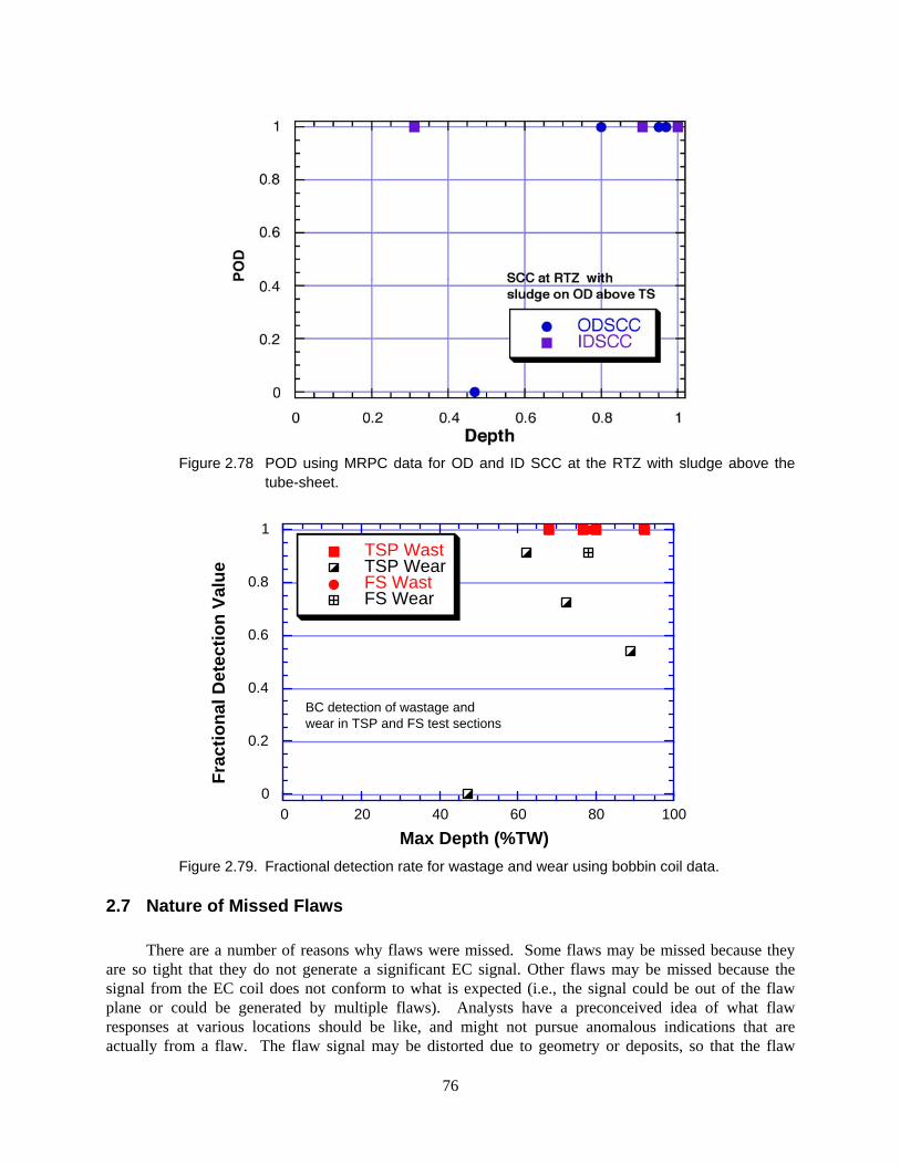
Figure 2.78 POD using MRPC data for OD and ID SCC at the RTZ with sludge above the

tube-sheet.

0

0.2

0.4

0.6

0.8

1

0 20 40 60 80 100

TSP WastTSP WearFS WastFS Wear

Fra

ctio

nal

Det

ecti

on

Val

ue

Max Depth (%TW)

BC detection of wastage and wear in TSP and FS test sections

Figure 2.79. Fractional detection rate for wastage and wear using bobbin coil data.

2.7 Nature of Missed Flaws

There are a number of reasons why flaws were missed. Some flaws may be missed because they are so tight that they do not generate a significant EC signal. Other flaws may be missed because the signal from the EC coil does not conform to what is expected (i.e., the signal could be out of the flaw plane or could be generated by multiple flaws). Analysts have a preconceived idea of what flaw responses at various locations should be like, and might not pursue anomalous indications that are actually from a flaw. The flaw signal may be distorted due to geometry or deposits, so that the flaw

76

signal is no longer recognized. Very long flaws may be missed because the analysts may concentrate on a small portion of the flaw, thereby missing the overall response. Confusion could also arise from conflicting behavior of two or more coils. For example, there could be a clear bobbin coil signal, but nothing reportable from an MRPC. Some cracks detectable with an MRPC are not detected by the bobbin coil.

Human factors are also clearly important. Some teams missed flaws that seem to have very clear signals. This may be related to analyst fatigue, but this is conjectural since no effort was made to track, e.g., when during the day an analysis of a particular indication was performed.

2.8 Nature of Overcalls

Overcalls are generally the result of the characteristic of certain coils to generate flaw–like signals from geometrical distortions and deposits. Overcalls could also be the result of confusion from conflicting behavior of two or more coils. In a round–robin exercise, participants tend to make calls that might not be made under field conditions because there is no penalty for overcalling as long as the overcalling is not abused. In fact, the reports from the resolution analysts show that, except for dents, the overcalling rates are low in the free–span (0.1%) and TSP (1.7%). Overcalling in the tube-sheet region is higher (6%). The complex nature of the roll transition is probably the root cause of the tube-sheet overcalling, although further review and destructive analysis suggest that some mechanical deformation of the tube may have occurred in the mock-up specimens at the tube-sheet level during tube expansion, flaw fabrication, and assembly.

77

3 Summary

The mock–up has been shown to have flaws similar to those in operating steam generators, and the RR exercise has successfully mimicked an in–service inspection from preparation of documentation, to collection of BC and MRPC data, to analysis of the data by qualified teams. Eleven teams have participated in the steam–generator RR exercise. The resolution analysts’ reports have been used to provide POD estimates for some flaw morphologies. The feasibility of determining the reference state (that is, estimating the maximum depth, average depth, area, and mp) from the eddy current profile of mock–up flaws has been validated through fractography of laboratory samples containing cracks with various morphologies similar to those in the mock–up and through the destructive analysis of some of the flaws from the mockup. The current NDE validation effort has led to POD estimates for axial and circumferential ID and OD SCC, shallow to deep. For the flaws analyzed, the mock–up POD is generally high for the deeper free–span and tube–support–plate SCCs. However, as noted previously, noise levels in the mock–up are generally less than in field data. Noise as severe as that sometimes observed, e.g., in the U–bends of operating steam generators, was not present in the mock–up free–span and TSP levels.

Most of the cracks in the mock–up are deep, as determined by the application of the multiparameter algorithm. The uncertainty in depth and the skewing toward deeper cracks are accounted for in the confidence limits associated with POD curves.

MRPC probes are more effective in characterizing defects than are BCs. For the tube-sheet where all test sections were examined by MRPC and BC, the MRPC POD is higher than the BC POD (see Figs. 2.62 and 2.63). In cases where MRPC examinations were performed following “I” code calls made with the bobbin coil, the resulting POD is lower than for the case of the BC. However, much of the apparent effectiveness of the BC is due to the conservative nature of the analyst’s calls and a potential for very high false call rates in some cases.

3.1 Bobbin Coil Results

The RR data and false call rates and the estimates of maximum depth were used to establish POD as a function of crack depth or mp and to generate logistic curve fits to the data. In general, the curves have a reasonable shape and thus provide plausible PODs (increasing POD with increasing depth). As expected, the POD for TSP ID cracks is higher than for OD cracks (95% with 93% OSL at 60% TW for IDSCC vs. 70% with 65% OSL at 60% TW for ODSCC). While as expected, the POD for free–span LODSCC (85% at 60% TW) is higher than that for TSP LODSCC (70% at 65% TW), it is lower than that for TSP LIDSCC (95% at 60% TW). The logistic fits using depths estimated by ANL’s multiparameter algorithm were compared to fits using the +Point maximum depth estimates. Using the +Point maximum depth estimates results led to a more conservative POD curve.

The NDE uncertainty in depth is included in the one–sided 95% lower confidence limit (OSL). However, these results only affect the uncertainty in the parameters of a particular model and do not account for the uncertainty in the choice of a model (e.g., linear logistic or log logistic). In some cases, because not enough flaws covering a complete range of depths were available and thus could be used to determine the goodness of the statistical fit reliably, the model uncertainty can be large. This uncertainty primarily affects the portion of the POD curves between about 25 to 80% TW.

In addition to determining POD as a function of flaw depth, the POD has been evaluated as a function of BC voltage for TSP LODSCC. The resulting curve was similar to the POPCD curved developed by industry.

78

The results were also analyzed by team to determine whether strong team–to–team variations existed in the POD. The performances of most of the teams cluster rather tightly, although in some cases significant variation occurred between best and worst. The probability that team–to–team variations in logistic fits to data are due to chance was estimated. For LIDSCC at the TSP, the variation from best to worst is very significant statistically. The probability is < 0.1% that the difference is due to chance (DTC). For FS OD, the variation from best to worst is likely to be significant (DTC is < 20%). For TSP OD, this variation is probably not significant (DTC > 60%).

The round–robin results for the small number of test sections with IGA were analyzed separately from the other flawed test sections. The results suggest that this type of volumetric cracking can be detected easily with a bobbin coil when the depth of attack is greater than 40% TW.

The BC results for EDM notches and laser cut slots have also been analyzed as a subset of the mock–up. For depths of 40% TW and greater, the success in detecting notches and laser cut slots is greater than for SCC of comparable depths. This finding suggests that POD curves generated using notches are unrealistically high for deep cracks.

3.2 Tube–Sheet MRPC Results

The POD has been calculated for SCC in the tube-sheet level of the mock–up with an MRPC. The maximum–likelihood logistic fit as a function of depth is presented in this report. For all TS POD curves, a false call rate of 6% was used. The OSLs included uncertainties in maximum depth.

For MRPC in the tube-sheet, the POD for inner–diameter SCC is ≈75%, with an OSL of ≈65%. The highest POD curve is for LIDSCC where the POD at 60% TW is 85%. Results are given for MRPC POD by team for axial and circumferential ID and OD SCC in the tube-sheet. The POD at 60% TW ranges from 80 to 60%.

Comparisons were made between the BC and MRPC PODs for the tube-sheet. For all SCCs, the POD curve is higher for the MRPC as might be expected. For tube–sheet LIDSCC only, the MRPC POD at 60% TW is 85%, while the BC POD is only 35%. For the tube-sheet, the MRPC is clearly the probe of choice for detection of SCCs. The complication of the roll transition and the presence of circumferential SCCs make separating the crack signals from geometry difficult when using a bobbin coil.

3.3 MRPC Analysis of TSP Signals

A review was performed of the practice of using the MRPC results for BC voltages between 2.0 and 5.6 V. Such calls are normally made to confirm or dismiss the BC flaw call. The result for LODSCC > 75% TW was an average correct call of 98%. However, results are less reliable for shallower cracks. All teams missed an LODSCC at the TSP with an estimated maximum depth of 39% TW. The signal from the +Point coil at 300 kHz for this crack was only a few tenths of a volt. This example illustrates the possibility of having a strong BC signal and a weak MRPC signal that would not be called a crack by analysts. Such situations could arise when a flaw is shallow and long, shallow and volumetric, or short and tight.

79

3.4 LIDSCC in Dented TSP

The BC and MRPC results for LIDSCC in dented TSP test sections have been analyzed as a subset of the mock–up (using resolution analyst reports). While there was a significant amount of overcalling of dents without SCC using the bobbin coil, the analysts were able to recognize the dents without cracking with the MRPC data.

3.5 Accuracy of Maximum Depth for Mock–up Cracks

Accuracy in estimating the maximum depth of cracks in the mock–up was determined by a comparison between crack profiles generated by ANL’s multiparameter algorithm and profiles determined from fractography. The overall RMSE for all cracks of all depths is 15.1%, but the RMSE varies significantly with depth. The RMSE value is significantly better for 80–100% TW cracks than for cracks with other depths.

Table 2.4 gives two sets of RMSE values. One set is based on the values obtained directly from the multiparameter algorithm and the other on “corrected” values obtained from the regression fit shown in Fig. 2.22. For the shallowest cracks, the “corrected” values give a significantly lower RMSE value, but when all the data are considered, the differences in the RMSE for corrected and uncorrected predictions are small. This finding indicates little systematic bias in the predictions of the multiparameter algorithm, i.e., the errors are random.

These sizing–accuracy results can be used to estimate the uncertainty in POD curves if the multiparameter algorithm is used to determine the “true” state of the mock–up for the NDE round–robin. Instead of characterizing the error in the depths in terms of the overall average for all depths (≈15%), the error was taken as a function of depth. Analytically, the RMSE values given in Table 2.3 are assumed to apply at the midpoint of the depth range for each bin. The error at other depths is then estimated by linear interpolation of these values.

3.6 Overall Capability

The detection capability of current ISI technology and procedures has been assessed by an eddy–current RR exercise with a mock–up of a steam–generator tube bundle. Inspection of the mock–up and analysis of the data mimicked industry ISI practices conducted on operating steam generators. All documentation for conducting the inspection was prepared with input from an industry–based NDE Task Group, and the realism of the mock–up was established. Data were acquired in June and August 1999, and the data were analyzed by 11 commercial teams in December 2000. Each team consisted of five qualified analysts. The exercise took seven to eight working days per team.

The conclusion from the RR results is that a good POD can be achieved for deep flaws when commercial techniques are used in a similar manner to the RR exercise. The level of success in detection of SCCs did vary with flaw location. The maximum depth from eddy current crack profiles and false call rates were estimated to establish POD as a function of depth and mp.

No useful correlation was found between signal amplitude or phase and the maximum depth of the mock–up flaws. When the PODs are considered as a function of mp in the TSP and FS regions, the POD for cracks that would fail or leak under 3p internal pressure (corresponding to mp ≈ 2.3) is > 95%, even when uncertainties are accounted for.

80

In sum, the adequacy of the multiparameter algorithm for obtaining profiles and maximum depth was established. The results of POD as a function of depth or mp were based on the profiles generated with this algorithm.

81

82

4 References

1. D. S. Kupperman, S. Bakhtiari, W. J. Shack, J. Y. Park, and S. Majumdar, Evaluation of Eddy Current Reliability from Steam Generator Mock–Up Round Robin ANL–01/22, U.S. Nuclear Regulatory Commission, Washington, DC (2002).

2. D. R. Diercks, S. Bakhtiari, K. E. Kasza, D. S. Kupperman, S. Majumdar, J. Y. Park, and W. J. Shack, Steam Generator Tube Integrity Program, Annual Report, October 1999–September 2000, NUREG/CR–6511, Vol. 8, U.S. Nuclear Regulatory Commission, Washington, DC (2002).

3. S. Bakhtiari, J. Y. Park, D. S. Kupperman, S. Majumdar, and W. J. Shack, Advanced NDE for Steam Generator Tubing, NUREG/CR–6746, U. S. Nuclear Regulatory Commission, Washington, DC (2001).

4. D. S. Kupperman, J. Y. Park, S. Majumdar, S. Bakhtiari, K. Kasza and W. J. Shack, Non-destructive and Failure Evaluation of Tubing from a Retired Steam Generator, NUREG/CR–6924, U.S. Nuclear Regulatory Commission, Washington, DC (2007).

5. S. Majumdar, K. Kasza, and J. Franklin, Pressure and Leak–Rate Tests and Models for Predicting Failure of Flawed Steam Generator Tubes, NUREG/CR–6664, U.S. Nuclear Regulatory Commission, Washington, DC (2000).

6. P. R. Bevington and D. K. Robinson, Data Reduction and Error Analysis for the Physical Sciences, 2nd Ed., McGraw Hill, New York (1992).

7. A. H. Bowker and G. J. Lieberman, Engineering Statistics, Prentice Hall, Englewood Cliffs, NJ (1972).

8. S. Bakhtiari, D. S. Kupperman, and W. J. Shack, Assessment of Noise Level for Eddy Current Inspection of Steam Generator Tubes, NUREG/CR–6982, U.S. Nuclear Regulatory Commission, Washington, DC (2009).

9. Special Report 06–02 – Results of Steam Generator (SG) Tube Inspections for Diablo Canyon Power Plant Unit 2 Thirteenth Refueling Outage. ML062400518 (2006)

Appendix A: Multiparameter Algorithm Profiles vs. Fractography

A1. Initial Set of SCC used for Validation

0

20

40

60

80

100

0 10 20 30 40 50 60 70

EC NDEFractography

Figure A1. AGL 2241 CODSCC: EC NDE depth versus position using the multiparameter algorithm (dotted curve) and fractography depth versus position (smooth curve).

Dep

th (

% T

W)

Crack Length (mm)

0

20

40

60

80

100

0 10 20 30 40 50 60 70

EC NDEFractography

Figure A2. AGL 2242 CIDSCC: EC NDE depth versus position using the multiparameter algorithm (dotted curve) and fractography depth versus position (smooth curve).

De

pth

(%

TW

)

Length (mm)

A–1

0.00

20.00

40.00

60.00

80.00

100.00

-10 0 10 20 30 40 50 60

EC NDEFractography

Figure A3. AGL 288 LIDSCC: EC NDE depth versus position using the multiparameter algorithm (dotted curve) and fractography depth versus position (smooth curve).

Dep

th (

% T

W)

Crack Length (mm)

0.00

20.00

40.00

60.00

80.00

100.00

120.00

20 25 30 35 40 45 50 55 60

EC NDEFractography


Dep

th (

% T

W)

Crack Length (mm)

0.00

20.00

40.00

60.00

80.00

100.00

120.00

-2 0 2 4 6 8 10 12

EC NDEFractography

Figure A5. AGL 533 LODSCC: EC NDE depth versus position using the multiparameter algorithm (dotted curve) and fractography depth versus position (smooth curve). D

epth

(%

TW

)

Crack Length (mm)

A–2

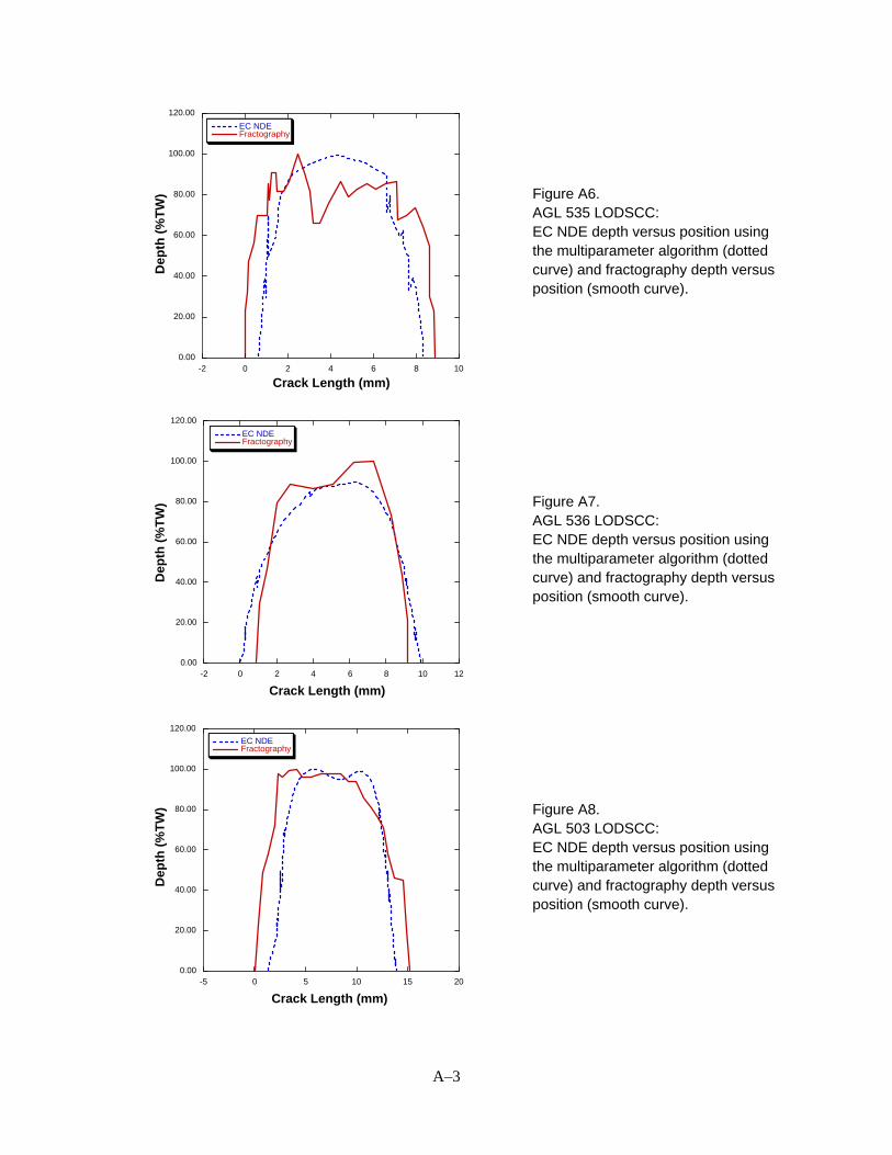
0.00

20.00

40.00

60.00

80.00

100.00

120.00

-2 0 2 4 6 8 10

EC NDEFractography

Figure A6. AGL 535 LODSCC: EC NDE depth versus position using the multiparameter algorithm (dotted curve) and fractography depth versus position (smooth curve).

Dep

th (

%T

W)

Crack Length (mm)

0.00

20.00

40.00

60.00

80.00

100.00

120.00

-2 0 2 4 6 8 10 12

EC NDEFractography


Dep

th (

%T

W)

Crack Length (mm)

0.00

20.00

40.00

60.00

80.00

100.00

120.00

-5 0 5 10 15 20

EC NDEFractography


Dep

th (

%T

W)

Crack Length (mm)

A–3

0.00

20.00

40.00

60.00

80.00

100.00

120.00

-5 0 5 10 15 20

EC NDEFractography


Dep

th (

%T

W)

Crack Length (mm)

0.00

20.00

40.00

60.00

80.00

100.00

-5 0 5 10 15 20

EC NDEFractography

Dep

th (

% T

W)

Crack Length (mm)


0.00

20.00

40.00

60.00

80.00

100.00

120.00

-10 0 10 20 30 40 50 60 70

EC NDEFractography


Dep

th (

% T

W)

Crack Length (mm)

A–4

0.00

20.00

40.00

60.00

80.00

100.00

120.00

-10 0 10 20 30 40 50 60 70

EC NDEFractography


De

pth

(%

TW

)

Crack Length (mm)

0.00

20.00

40.00

60.00

80.00

100.00

120.00

-10 0 10 20 30 40 50 60

EC NDEFractography


Dep

th (

%T

W)

Crack Length (mm)

0.00

20.00

40.00

60.00

80.00

100.00

0 10 20 30 40 50

EC NDEFractography


Dep

th (

% T

W)

Crack Length (mm)

A–5

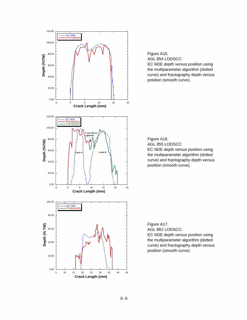
0.00

20.00

40.00

60.00

80.00

100.00

120.00

-5 0 5 10 15 20

EC NDEFractography


Dep

th (

%T

W)

Crack Length (mm)

0.00

20.00

40.00

60.00

80.00

100.00

120.00

-5 0 5 10 15 20 25

EC NDEFractographyFractography

Dep

th (

%T

W)

Crack Length (mm)

1 mm Off-setLigament

Crack A Crack B


0.00

20.00

40.00

60.00

80.00

100.00

5 10 15 20 25 30 35 40 45

EC NDEFractography


De

pth

(%

TW

)

Crack Length (mm)

A–6

0

20

40

60

80

100

120

-5 0 5 10 15 20 25 30 35

EC NDEFractography

Dep

th (

%T

W)

Crack Length (mm)


0.00

20.00

40.00

60.00

80.00

100.00

0 5 10 15 20

EC NDEFractography


Dep

th (

% T

W)

Crack Length (mm)

0

20

40

60

80

100

120

0 20 40 60 80

EC NDEFractography


Dep

th (

%T

W)

Crack Length (mm)

A–7

0

20

40

60

80

100

-5 0 5 10 15 20

EC NDEFractography


Dep

th (

% T

W)

crack Length (mm)

0.00

20.00

40.00

60.00

80.00

100.00

-10 0 10 20 30 40 50 60

EC NDEFractography


Dep

th (

% T

W)

Crack Length (mm)

0.00

20.00

40.00

60.00

80.00

100.00

0 5 10 15 20

EC NDEFractography


Dep

th (

% T

W)

Crack Length (mm)

A–8

A2. Subset of 13 additional cracks from the mock-up.

0

20

40

60

80

100

-5 0 5 10 15 20 25 30 35

EC NDEFractography

Dep

th (

% T

W)

Length (mm)

CODSCC

Figure A24. Test section 42 removed from mock–up with a CODSCC. EC NDE depth versus position using the multiparameter algorithm (dotted curve) and fractography depth versus position (smooth curve).

0

20

40

60

80

100

-5 0 5 10 15 20 25 30

EC NDEFractography

Dep

th (

% T

W)

Length (mm)

CODSCC


A–9

0

20

40

60

80

100

-5 0 5 10 15 20 25 30

EC NDEFractography

Dep

th (

% T

W)

Length (mm)

CODSCC


0

20

40

60

80

100

-10 0 10 20 30

EC NDEFractography

Dep

th (

% T

W)

Length (mm)

LODSCC

Figure A27. Test section 44 removed from mock–up with an LODSCC. EC NDE depth versus position using the multiparameter algorithm (dotted curve) and fractography depth versus position (smooth curve).

A–10

0

20

40

60

80

100

120

0 5 10 15 20 25 30

EC NDEFractography

Dep

th (

% T

W)

Length (mm)

LODSCC


0

20

40

60

80

100

120

-5 0 5 10 15 20

EC NDEFractography

Dep

th (

% T

W)

Length (mm)

LODSCC


A–11

0

20

40

60

80

100

120

-5 0 5 10 15 20 25

EC NDEFractography

Dep

th (

% T

W)

Length (mm)

LODSCC


A–12

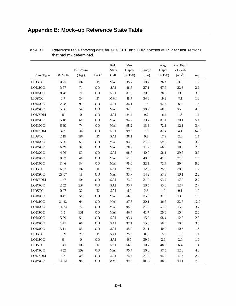
Appendix B: Mock–up Reference State Table

Table B1. Reference table showing data for axial SCC and EDM notches at TSP for test sections that had mp determined.

Flaw Type

BC Volts

BC Phase

(deg.)

ID/OD

Ref.

State

Call

Max

Depth

(% TW)

Length

(mm)

Avg.

Depth

(% TW)

Ave. Depth

x Length

(mm2)

mp

LIDSCC 9.97 107 ID MAI 35.2 10.7 26.4 3.5 1.2

LODSCC 3.57 71 OD SAI 88.8 27.1 67.6 22.9 2.6

LODSCC 8.78 70 OD SAI 87.8 20.0 78.8 19.6 3.6

LIDSCC 2.7 24 ID MMI 45.7 34.2 19.2 8.1 1.2

LODSCC 2.28 91 OD SAI 84.1 7.8 62.7 6.0 1.5

LODSCC 5.56 59 OD MAI 94.5 30.2 68.5 25.8 4.5

LODEDM 0 0 OD SAI 24.4 9.2 16.4 1.8 1.1

LODSCC 5.18 68 OD MAI 94.2 29.7 81.4 30.1 5.4

LODSCC 6.69 74 OD MAI 95.2 13.6 72.1 12.1 3.4

LODEDM 4.7 36 OD SAI 99.8 7.0 82.4 4.1 34.2

LIDSCC 2.19 187 ID SAI 28.1 9.5 17.3 2.0 1.1

LODSCC 5.56 63 OD MAI 93.8 21.0 69.8 16.5 3.2

LODSCC 6.49 39 OD MAI 78.9 21.9 66.0 18.0 2.3

LODSCC 4.76 53 OD SAI 98.7 40.7 58.1 29.5 3.3

LODSCC 0.63 46 OD MAI 61.3 40.5 41.5 21.0 1.6

LODSCC 3.46 54 OD MAI 95.0 32.5 72.4 29.4 5.2

LIDSCC 6.02 187 ID SAI 29.5 12.0 25.5 38.3 1.2

LODSCC 29.07 18 OD MAI 93.7 14.2 57.3 10.1 2.2

LODEDM 1.47 104 OD SAI 73.5 21.6 63.9 17.3 2.2

LODSCC 2.52 134 OD SAI 93.7 18.5 53.8 12.4 2.4

LIDSCC 0.97 32 ID SAI 4.0 2.6 1.9 0.1 1.0

LODSCC 0.47 58 OD MAI 66.5 35.0 31.2 13.6 1.6

LODSCC 21.42 64 OD MAI 97.8 30.1 86.6 32.5 12.0

LODSCC 16.74 77 OD MAI 95.6 21.6 57.5 15.5 3.7

LODSCC 1.5 131 OD MAI 86.4 41.7 29.6 15.4 2.3

LODSCC 5.89 51 OD SAI 93.4 15.0 68.4 12.8 2.3

LODSCC 1.41 66 OD SAI 97.4 15.8 50.8 10.0 3.5

LODSCC 3.11 53 OD SAI 85.0 21.1 40.0 10.5 1.8

LIDSCC 1.09 25 ID SAI 25.5 8.0 15.5 1.5 1.1

LODSCC 0 0 OD SAI 9.5 59.8 2.8 2.0 1.0

LIDSCC 1.41 103 ID SAI 66.9 10.7 48.2 6.4 1.4

LODSCC 4.53 192 OD MAI 99.4 16.8 57.5 12.0 4.8

LODEDM 3.2 89 OD SAI 74.7 21.9 64.0 17.5 2.2

LODSCC 19.84 90 OD MMI 97.5 283.7 80.0 24.1 7.7

B–1

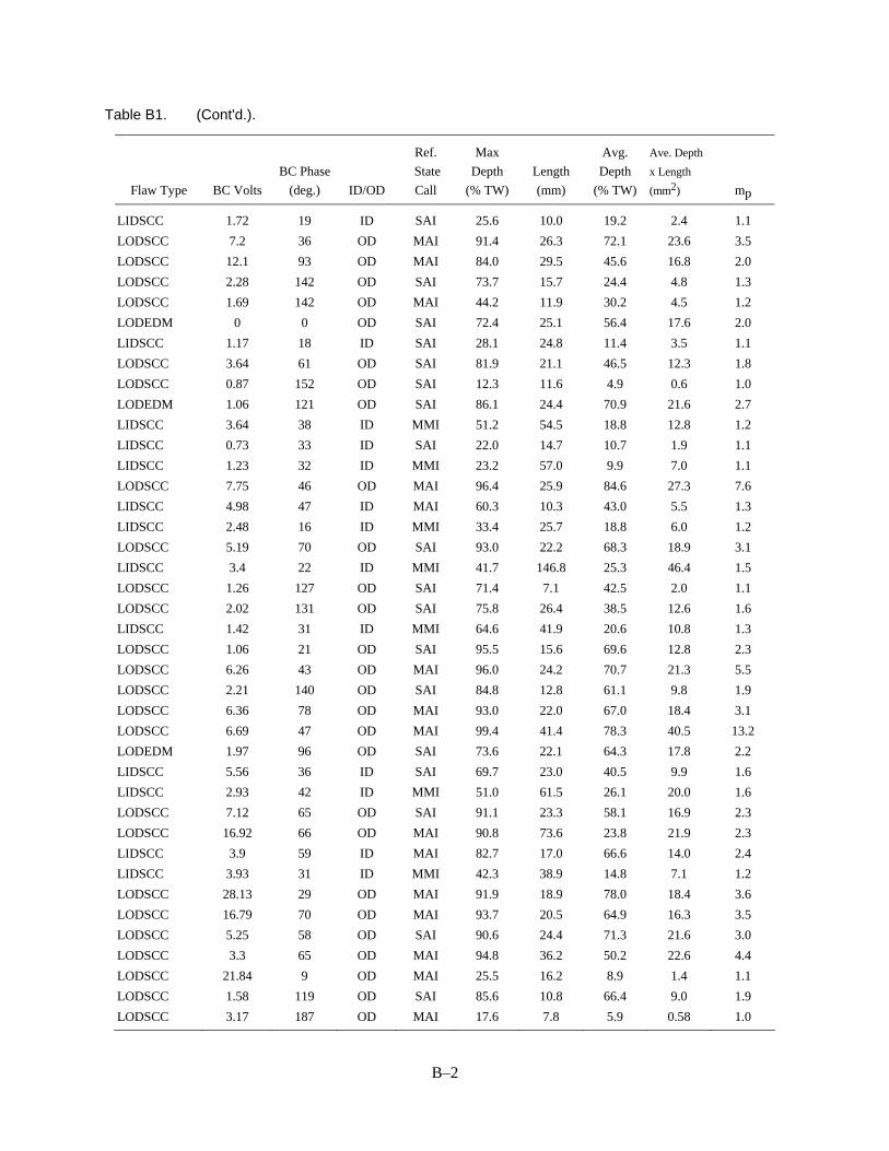
Table B1. (Cont'd.).

Flaw Type

BC Volts

BC Phase

(deg.)

ID/OD

Ref.

State

Call

Max

Depth

(% TW)

Length

(mm)

Avg.

Depth

(% TW)

Ave. Depth

x Length

(mm2)

mp

LIDSCC 1.72 19 ID SAI 25.6 10.0 19.2 2.4 1.1

LODSCC 7.2 36 OD MAI 91.4 26.3 72.1 23.6 3.5

LODSCC 12.1 93 OD MAI 84.0 29.5 45.6 16.8 2.0

LODSCC 2.28 142 OD SAI 73.7 15.7 24.4 4.8 1.3

LODSCC 1.69 142 OD MAI 44.2 11.9 30.2 4.5 1.2

LODEDM 0 0 OD SAI 72.4 25.1 56.4 17.6 2.0

LIDSCC 1.17 18 ID SAI 28.1 24.8 11.4 3.5 1.1

LODSCC 3.64 61 OD SAI 81.9 21.1 46.5 12.3 1.8

LODSCC 0.87 152 OD SAI 12.3 11.6 4.9 0.6 1.0

LODEDM 1.06 121 OD SAI 86.1 24.4 70.9 21.6 2.7

LIDSCC 3.64 38 ID MMI 51.2 54.5 18.8 12.8 1.2

LIDSCC 0.73 33 ID SAI 22.0 14.7 10.7 1.9 1.1

LIDSCC 1.23 32 ID MMI 23.2 57.0 9.9 7.0 1.1

LODSCC 7.75 46 OD MAI 96.4 25.9 84.6 27.3 7.6

LIDSCC 4.98 47 ID MAI 60.3 10.3 43.0 5.5 1.3

LIDSCC 2.48 16 ID MMI 33.4 25.7 18.8 6.0 1.2

LODSCC 5.19 70 OD SAI 93.0 22.2 68.3 18.9 3.1

LIDSCC 3.4 22 ID MMI 41.7 146.8 25.3 46.4 1.5

LODSCC 1.26 127 OD SAI 71.4 7.1 42.5 2.0 1.1

LODSCC 2.02 131 OD SAI 75.8 26.4 38.5 12.6 1.6

LIDSCC 1.42 31 ID MMI 64.6 41.9 20.6 10.8 1.3

LODSCC 1.06 21 OD SAI 95.5 15.6 69.6 12.8 2.3

LODSCC 6.26 43 OD MAI 96.0 24.2 70.7 21.3 5.5

LODSCC 2.21 140 OD SAI 84.8 12.8 61.1 9.8 1.9

LODSCC 6.36 78 OD MAI 93.0 22.0 67.0 18.4 3.1

LODSCC 6.69 47 OD MAI 99.4 41.4 78.3 40.5 13.2

LODEDM 1.97 96 OD SAI 73.6 22.1 64.3 17.8 2.2

LIDSCC 5.56 36 ID SAI 69.7 23.0 40.5 9.9 1.6

LIDSCC 2.93 42 ID MMI 51.0 61.5 26.1 20.0 1.6

LODSCC 7.12 65 OD SAI 91.1 23.3 58.1 16.9 2.3

LODSCC 16.92 66 OD MAI 90.8 73.6 23.8 21.9 2.3

LIDSCC 3.9 59 ID MAI 82.7 17.0 66.6 14.0 2.4

LIDSCC 3.93 31 ID MMI 42.3 38.9 14.8 7.1 1.2

LODSCC 28.13 29 OD MAI 91.9 18.9 78.0 18.4 3.6

LODSCC 16.79 70 OD MAI 93.7 20.5 64.9 16.3 3.5

LODSCC 5.25 58 OD SAI 90.6 24.4 71.3 21.6 3.0

LODSCC 3.3 65 OD MAI 94.8 36.2 50.2 22.6 4.4

LODSCC 21.84 9 OD MAI 25.5 16.2 8.9 1.4 1.1

LODSCC 1.58 119 OD SAI 85.6 10.8 66.4 9.0 1.9

LODSCC 3.17 187 OD MAI 17.6 7.8 5.9 0.58 1.0

B–2

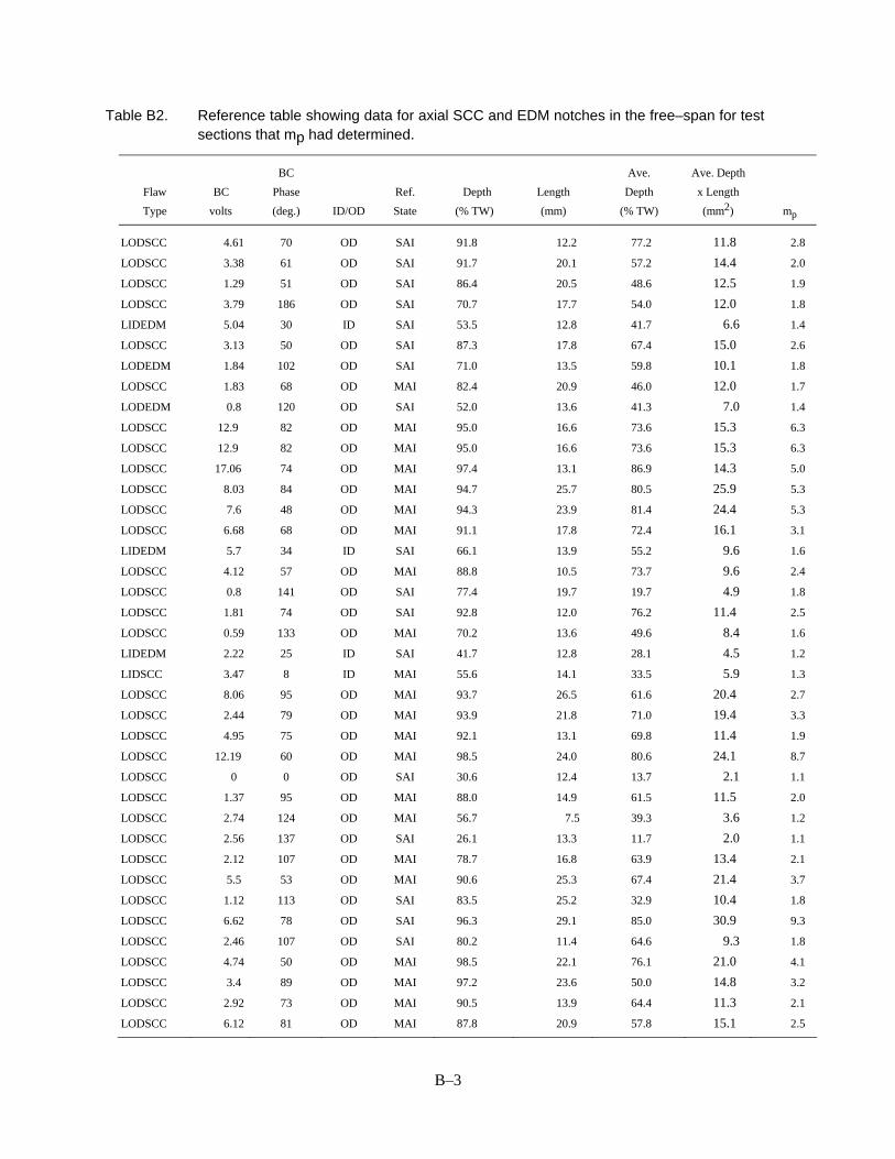
Table B2. Reference table showing data for axial SCC and EDM notches in the free–span for test sections that mp had determined.

Flaw

Type

BC

volts

BC

Phase

(deg.)

ID/OD

Ref.

State

Depth

(% TW)

Length

(mm)

Ave.

Depth

(% TW)

Ave. Depth

x Length

(mm2)

mp

LODSCC 4.61 70 OD SAI 91.8 12.2 77.2 11.8 2.8

LODSCC 3.38 61 OD SAI 91.7 20.1 57.2 14.4 2.0

LODSCC 1.29 51 OD SAI 86.4 20.5 48.6 12.5 1.9

LODSCC 3.79 186 OD SAI 70.7 17.7 54.0 12.0 1.8

LIDEDM 5.04 30 ID SAI 53.5 12.8 41.7 6.6 1.4

LODSCC 3.13 50 OD SAI 87.3 17.8 67.4 15.0 2.6

LODEDM 1.84 102 OD SAI 71.0 13.5 59.8 10.1 1.8

LODSCC 1.83 68 OD MAI 82.4 20.9 46.0 12.0 1.7

LODEDM 0.8 120 OD SAI 52.0 13.6 41.3 7.0 1.4

LODSCC 12.9 82 OD MAI 95.0 16.6 73.6 15.3 6.3

LODSCC 12.9 82 OD MAI 95.0 16.6 73.6 15.3 6.3

LODSCC 17.06 74 OD MAI 97.4 13.1 86.9 14.3 5.0

LODSCC 8.03 84 OD MAI 94.7 25.7 80.5 25.9 5.3

LODSCC 7.6 48 OD MAI 94.3 23.9 81.4 24.4 5.3

LODSCC 6.68 68 OD MAI 91.1 17.8 72.4 16.1 3.1

LIDEDM 5.7 34 ID SAI 66.1 13.9 55.2 9.6 1.6

LODSCC 4.12 57 OD MAI 88.8 10.5 73.7 9.6 2.4

LODSCC 0.8 141 OD SAI 77.4 19.7 19.7 4.9 1.8

LODSCC 1.81 74 OD SAI 92.8 12.0 76.2 11.4 2.5

LODSCC 0.59 133 OD MAI 70.2 13.6 49.6 8.4 1.6

LIDEDM 2.22 25 ID SAI 41.7 12.8 28.1 4.5 1.2

LIDSCC 3.47 8 ID MAI 55.6 14.1 33.5 5.9 1.3

LODSCC 8.06 95 OD MAI 93.7 26.5 61.6 20.4 2.7

LODSCC 2.44 79 OD MAI 93.9 21.8 71.0 19.4 3.3

LODSCC 4.95 75 OD MAI 92.1 13.1 69.8 11.4 1.9

LODSCC 12.19 60 OD MAI 98.5 24.0 80.6 24.1 8.7

LODSCC 0 0 OD SAI 30.6 12.4 13.7 2.1 1.1

LODSCC 1.37 95 OD MAI 88.0 14.9 61.5 11.5 2.0

LODSCC 2.74 124 OD MAI 56.7 7.5 39.3 3.6 1.2

LODSCC 2.56 137 OD SAI 26.1 13.3 11.7 2.0 1.1

LODSCC 2.12 107 OD MAI 78.7 16.8 63.9 13.4 2.1

LODSCC 5.5 53 OD MAI 90.6 25.3 67.4 21.4 3.7

LODSCC 1.12 113 OD SAI 83.5 25.2 32.9 10.4 1.8

LODSCC 6.62 78 OD SAI 96.3 29.1 85.0 30.9 9.3

LODSCC 2.46 107 OD SAI 80.2 11.4 64.6 9.3 1.8

LODSCC 4.74 50 OD MAI 98.5 22.1 76.1 21.0 4.1

LODSCC 3.4 89 OD MAI 97.2 23.6 50.0 14.8 3.2

LODSCC 2.92 73 OD MAI 90.5 13.9 64.4 11.3 2.1

LODSCC 6.12 81 OD MAI 87.8 20.9 57.8 15.1 2.5

B–3

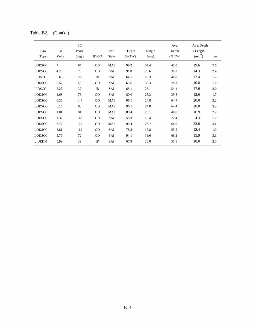
B–4

Table B2. (Cont'd.)

Flaw

Type

BC

Volts

BC

Phase

(deg.)

ID/OD

Ref.

State

Depth

(% TW)

Length

(mm)

Ave.

Depth

(% TW)

Ave. Depth

x Length

(mm2) mp

LODSCC 7 65 OD MAI 99.2 37.4 42.0 19.6 7.5

LODSCC 4.28 70 OD SAI 91.8 28.6 39.7 14.3 2.4

LIDSCC 0.68 110 ID SAI 64.1 20.3 48.8 12.4 1.7

LODSCC 0.57 45 OD SAI 65.5 30.3 28.3 10.8 1.4

LIDSCC 5.27 37 ID SAI 68.1 26.1 54.1 17.6 2.0

LODSCC 1.68 76 OD SAI 80.0 25.3 39.8 12.6 1.7

LODSCC 0.36 144 OD MAI 96.1 24.8 64.4 20.0 3.2

LODSCC 6.15 68 OD MAI 96.1 24.8 64.4 20.0 3.2

LODSCC 1.01 81 OD MAI 80.4 28.1 48.0 16.9 2.2

LODSCC 1.37 148 OD SAI 58.3 12.4 27.4 4.3 1.2

LODSCC 6.77 129 OD MAI 90.4 28.7 66.0 23.6 3.1

LODSCC 8.81 169 OD SAI 78.2 17.8 55.5 12.4 1.9

LODSCC 5.76 72 OD SAI 94.1 18.6 68.2 15.9 3.3

LIDEDM 5.99 39 ID SAI 67.3 25.8 55.8 18.0 2.0

Appendix C: Examination Technique Specification Sheets

Examination Technique Specification Sheet for Bobbin Coil

ETSS #1 BOBBIN PROBE ACQUISITION Revision 6 Site: Argonne SG Mock–up Page 1 of 5

Examination Scope Applicability: Standard ASME Code examination for tubing. Detection of IGA/ODSCC in free–span with and without sludge, at nondented drilled TSPs, and above the TS sludge pile region. Detection of axial PWSCC at dented drilled tube support plate intersections, wastage and wear. This technique meets the requirements of App. H ETSSs 96001, 96004 (except sizing), 96007 and 96008 and 96012. Instrument Tubing

Manufacturer/Model: Zetec MIZ–30, Tecrad TC6700 Material Type: Inconel 600

Data Recording Equipment OD X Wall (inch): 0.875 X 0.050

Manuf./Media: HP Hard Drive, 2.6 Gb Optical or Equiv. Calibration Standard

Software Type: ASME Rev. 5 requirements

Manufacturer: Zetec or Westinghouse latest approved version Analog Signal Path Probe Extension Manuf.: Zetec

Examination Procedure Extension Type & Length: Universal 940–1760, 50 ft.

Number/Revision: ANL002/Rev. 3 Slip Ring Model Number: 508–2052 or equivalent

Scan Parameters

Scan Direction: Pull

Digitization Rate, Samples Per Inch (minimum): Axial Direction 37 Circ. Direction N/A

Nominal Probe Speed Sample Rate RPM Set RPM Recommended Min

RPM Recommended

21”/sec. 800 N/A N/A N/A

Probe/Motor Unit

Description (Model/Diameter/Coil Dimensions) Manufacturer/Part Number Length

A–720–M/ULC (720UL) Zetec 760–1192–000 110 ft.

Data Acquisition

Calibration Coil 1 Channels Frequency Channel

400 kHz Ch.1

200 kHz Ch. 3

100 kHz Ch. 5

20 kHz Ch. 7

Phase Rotation

100% TWH 40 degrees

100% TWH 40 degrees

100% TWH 40 degrees

TSP 270 Degrees

Span Setting

100% TWH 5 divisions



TSP 5 divisions

Calibration Coil 5 Channels

Frequency Channel

400 kHz Ch. 2

200 kHz Ch. 4

100 kHz Ch. 6

20 kHz Ch. 8

Phase Rotation

100% TWH 40 degrees

100% TWH 40 degrees

100% TWH 40 degrees

TSP 270 Degrees

Span Setting




TSP 5 divisions

C–1

ETSS#1 BOBBIN PROBE ACQUISITION Revision 6

Site: Argonne SG Mock–up Page 2 of 5

Configuration Board Settings

trig: off down configuration#:0 name:Bobbin samples/sec:see pg1 rec.media = HD

tester= board#1 board#2 board#3 board#4 board#5

#of channels= 8 probe#1 probe#1 probe#2 probe#2 probe#1

DRIVE DRIVE DRIVE DRIVE DRIVE

A D B C A D B C A D B C A D B C A D B C

Drive Polarity N N

Group Number 1 1

Coil Number 1 5

freq#1 Time slot #1

400kHz G:x2 12.0V D A

freq#2 Time slot#2

200kHz G:x2 12.0V D A

freq#3 Time slot#3

100kHz G:x2 12.0V D A

freq#4 Time slot#4

20kHz G:x2 12.0V D A

freq#5 Time slot#5

End loc ch: 1 1 driveA: D=A1–A2, P=dr.A1 pu:A2, DP= dr: D1&D2 pu:A1&A2

Threshold off off driveB: D=B1–B2, A=A1–A2

(P) Gain x6 P=dr: B1 pu:B2, DP = dr:C1&C2 pu: B1&B2

Active Probes 1 drive C:D=C1– C2, A=D1–C2

(see note 1) drive D:D= D1–D2

Special Instructions

1. The 720MULC probe is the primary use probe for the bobbin examination.

2. Examine each tube full length or to the extent possible.

3. Three recordings of the calibration standard should be performed at the beginning and end of

each calibration group or every four hours, whichever comes first.

4. Periodically monitor all channels for data quality and acceptability.

C–2

Examination Technique Specification Sheet

ETSS#1– BOBBIN PROBE ANALYSIS Revision 6 Page: 3 of 5

Data Analysis

Calibration Differential Channels

Channels & Ch 1 Ch 3 Ch 5 Ch 7

Frequency 400 kHz 200 kHz 100 kHz 20 kHz

Phase Rotation 100% TWH 100% TWH 100% TWH TSP

40±1° 40±1° 40±1° 270±3°

Span Setting 4x20FBH @ 4 Div 4x20FBH @ 4 Div 4x20FBH @ 4 Div TSP

Minimum 5 divisions

Calibration Absolute Channels

Channel & Ch 2 Ch 4 Ch 6 Ch 8

Frequency 400 kHz 200 kHz 100 kHz 20 kHz

Phase Rotation Probe Motion Horiz. Probe Motion Horiz. Probe Motion Horiz. TSP

Flaws Up Flaws Up Flaws Up 270±3°

Span Setting 100% TWH 100% TWH 100% TWH TSP

Minimum 2 divisions 2 divisions 2 divisions 5 divisions

Calibration Process and Other Channels

Channels & P1(Ch 1/5) P2(Ch 2/6) P3(Ch 3/1/5)

Frequency 400/100 kHz Diff 400/100 kHz ABS 200/400/100 kHz Diff

Configure & Suppress Suppress Save 100,60,20

Adjust Drilled TSP Drilled TSP Suppress Drilled

Parameters TSP, Expansion

Phase Rotation 100% TWH 100% TWH 100% TWH

~35° , noise horiz. ~35°, noise horiz. @40±3°

Span Setting 4x20 FBH 100% TWH 100% TWH

Minimum @ 4 divisions 2 divisions 5 divisions

Voltage Normalization Calibration Curves

CH Signal Set Normalize Type CH Set Points

1 4X20% FBH 4.0 volts All Phase 1,3,5,P1 Max Rate 100,60,20,FBH

Curve 2,4,6,P2 Vpp (use as–built dimens)

Data Screening

Left Strip Chart Right Strip Chart Lissajous

P1 Ch 6 P1

Reporting Requirements

Condition/Region Report Ch Comment

Free–span NQI P1 All indications

Absolute Drift ADI 6 Gradual indications that lack a differential response

Drilled TSP DSI P1 All indications within TSP

Tubesheet Interface DTI P1 Distorted Top of Tubesheet

Dent(Structure) DNT P1(Vpp) Report all Dents > 2.0 volts at TSP's or TS interface

Ding(Free–span) DNG P1(Vpp) Report all Dings in free–span > 2.00 volts

Dent/Ding with ind. DNI P1 Distorted dent/ding with possib. indication of degrad

ID Chatter or Pilger. IDC P1 Any indication which you believe could mask an indic.

Permeability Variat. PVN P1 Any indication which you believe could mask an indic.

C–3

Examination Technique Specification Sheet ETSS# 1– Bobbin Probe Analysis Revision 6 Page 4 of 5


1. Provide a best estimate of % TW on all bobbin indications based on ASME calibration curve. Place appropriate "I–Code" in the Utility 1 field. Place flaw origin in Util 2 (ID or OD). 2. Zoom the strip charts to 3 (or equivalent setting based on window size) for increased visibility of small amplitude indications. 3. Scroll each free–span region with channel 3. 4. Scroll each top of tube–sheet region and expansion transition with channel P1 and P3. 5. Review each drilled TSP with channel P1 and Channel 3. 6. Monitor the 100 kHz absolute strip chart for positive drift. 7. Refer to the flow chart on the following page for additional information on evaluation of indications. 8. When distorted indications within dents or dings are identified, record the dent voltage as well as the indication. 9. All data should be analyzed unless voided by the operator. There are no retest codes necessary for the mock–up. Use BDA for bad data. 10. Landmarking is not necessary. All elevations will be recorded by data point. 11. Graphics are not required. 12. Do not report signals within one inch of test section ends.

C–4

Report as NQI on P1

ETSS#1-Bobbin Probe Revision 6 Page 5 of 5


Bobbin Probe Flow Chart

Differential Signal

yes

Indication Located Within or Influenced by a TSP

Report %TW on Process Channel P1

yes

yes

Report as DSI in UTIL 1 and ID or OD in Util 2

Examine with MRPC

Indications of possible degradation located at a TS expansion transition shall be reported as DTI using P1 regardless of any correlation in this Logic Flow

NoChange Test Mode

*Absolute Signal

No Indication Located at the TS Expansion Region

No Indication Located in Free Span

yes

Report %TW Indication with P1

yes

Report as DTI in UTIL 1 and ID or OD in Util 2

Indication Measures %TW on Channel 3

yes

yes

Indication Shows Logical Phase Rotation Between Chs 1,3,5 and Displays a Response on P1

yes

Report %TW on Ch. P1, "I" Code in UTIL 1, ID or OD in Util 2

Go to Absolute Signal *

yes

Report %TW on Highest Frequency Channel

yes

Report as ADI in Util 1 and ID or OD in Util 2

No

NDD

Examine with MRPC and evaluate the morphology

Phase Influence where an accurate %TW cannot be made

No

No yes

No

C–5

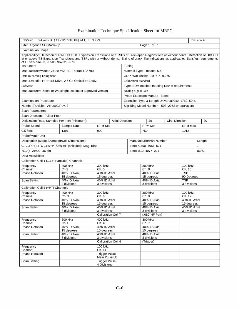
Examination Technique Specification Sheet for MRPC

ETSS #2 3–Coil RPC (.115/+PT/.080 HF) ACQUISITION Revision 6

Site: Argonne SG Mock–up Page 1 of 7

Examination Scope

Applicability: Detection of PWSCC at TS Expansion Transitions and TSPs or Free–span Regions with or without dents. Detection of ODSCC at or above TS Expansion Transitions and TSPs with or without dents. Sizing of crack–like indications as applicable. Satisfies requirements of ETSSs, 96403, 96508, 96702, 96703. Instrument Tubing

Manufacturer/Model: Zetec MIZ–30, Tecrad TC6700 Material Type: Inconel 600

Data Recording Equipment OD X Wall (inch): 0.875 X 0.050

Manuf./Media: HP Hard Drive, 2.6 Gb Optical or Equiv. Calibration Standard

Software Type: EDM notches meeting Rev. 5 requirements

Manufacturer: Zetec or Westinghouse latest approved version Analog Signal Path

Probe Extension Manuf.: Zetec

Examination Procedure Extension Type & Length:Universal 940–1760, 50 ft.

Number/Revision: ANL002/Rev. 3 Slip Ring Model Number: 508–2052 or equivalent

Scan Parameters

Scan Direction: Pull or Push

Digitization Rate, Samples Per Inch (minimum): Axial Direction 30 Circ. Direction 30

Probe Speed Sample Rate RPM Set RPM Min RPM Max

0.5”/sec. 1391 900 750 1012

Probe/Motor Unit

Description (Model/Diameter/Coil Dimensions) Manufacturer/Part Number Length

0.720(775) 3–C 115/+PT/080 HF (shielded), Mag–Bias Zetec C700–4055–071 .

.610(5–2)M/U–36 pin Zetec 810–4077–001 83 ft.

Data Acquisition

Calibration Coil 1 (.115" Pancake) Channels

Frequency Channel

400 kHz Ch.2

300 kHz Ch. 5

200 kHz Ch. 8

100 kHz Ch. 10

Phase Rotation

40% ID Axial 15 degrees



TSP 90 Degrees

Span Setting

40% ID Axial 3 divisions



TSP 3 divisions

Calibration Coil 5 (+PT) Channels

Frequency Channel

400 kHz Ch. 3

300 kHz Ch. 6

200 kHz Ch. 9

100 kHz Ch. 12

Phase Rotation





Span Setting





Calibration Coil 7 (.080"HF Pan)

Frequency Channel

600 kHz Ch.1

400 kHz Ch. 4

300 kHz Ch. 7

Phase Rotation




Span Setting




Calibration Coil 4 (Trigger)

Frequency Channel

100 kHz Ch. 11

Phase Rotation Trigger Pulse Main Pulse Up

Span Setting

Trigger Pulse 4 Divisions

C–6


ETSS#2 – 3–Coil RPC (.115/+PT/.080) Revision 6 Page: 2 of 7

Configuration Board Settings

trig: off down configuration#:0 name: samples/sec:see page 1 rec.media = HD

tester= board#1 board#2 board#3 board#4 board#5

#of channels= 12 probe#1 probe#1 probe#3 probe#4 probe#5

DRIVE DRIVE DRIVE DRIVE DRIVE

A D B C A D B C A D B C A D B C A D B C

Drive Polarity N N N N N

Group Number 1 1 1 1 1

Coil Number 1 4 5 7 8

freq#1 Time slot #1

600kHz G:x2 12.0V D

freq#2 Time slot#2

400kHz G:x2 12.0V D D D

freq#3 Time slot#3

300kHz G:x2 12.0V D D D

freq#4 Time slot#4

200kHz G:x2 12.0V D D

freq#5 Time slot#5

100kHz G:x2 12.0V D D D


1. One calibration standard may be recorded at the beginning and end of each cal group provided

it is a successful scan of the standards’ complete length.

2. Data will be recorded on the PUSH when running top of tube–sheet exams. Data recorded on the

PUSH is acceptable for other regions of the mock–up. The operator shall state the direction of

scanning in a message.

3. All locations shall be acquired from structure to structure unless an encoder is used. When an

encoder is used the location may be acquired from the respective structure to a few inches past

the area of interest. Care should be taken to insure that the proper location is scanned with

adequate data past the target location to account for any variations in probe speed or axial

scaling.

4. Tubes that have been mis–encoded should be corrected by entering a message to void that entry

and re–examining the tube with the proper encode.

5. Periodically monitor all channels for data quality and acceptability.

C–7


ETSS#2–3 Coil RPC (.115/+PT/.080) Analysis Revision 6 Page: 3 of 7

Data Analysis


Channels & Ch 2 Ch 5 Ch 8 Ch 10 Frequency 400 kHz 115MR 300 kHz 115MR 200 kHz 115MR 100 kHz 115MR

Phase Rotation 40% ID Axial 40% ID Axial 40% ID Axial 40% ID Axial 15±1° 15±1° 15±1° 15±1°

Span Setting 40% ID Axial 40% ID Axial 40% ID Axial 40% ID Axial Minimum 3 divisions 3 divisions 3 divisions 3 divisions


Channel & Ch 3 Ch 6 Ch 9 Ch 12 Frequency 400 kHz+Axial 300 kHz+Axial 200 kHz+Axial 100 kHz+Axial

Phase Rotation 40%ID Axial 40%ID Axial 40%ID Axial 40%ID Axial 15°±1° 15°±1° 15°±1° 15°±1°

Span Setting 40% ID Axial 40% ID Axial 40% ID Axial 40%ID Axial Minimum 3 divisions 3 divisions 3 divisions 3 divisions

Calibration Coil 7(.080" HF Pancake)

Channels & Ch 1 Ch 4 Ch 7 Frequency 600 kHz 080HF 400 kHz 080HF 300 kHz 080HF

Phase Rotation 40%ID Axial 40%ID Axial 40%ID Axial 15°±1° 15°±1° 15°±1°

Span Setting 40%ID Axial 40%ID Axial 40%ID Axial Minimum 3 divisions 3 divisions 3 divisions

Calibration Coil 4 (Trigger) Channels

Channel & Ch 11 Frequency 100 kHz TRIG


Span Setting Trigger Pulse Minimum 4 divisions

Calibration Process Channels

Channels & Ch P1(Ch 3) Ch P2 (Ch 6) Ch P3 (Ch 9) Ch P4 (Ch 12) Frequency 400 kHz + CIRC 300 kHz+CIRC 200 kHz +CIRC 100 kHz + CIRC

Adjust Parameters N/A N/A N/A N/A

Phase Rotation 40%ID Circ 40%ID Circ 40%ID Circ 40%ID Circ 15°±1° 15°±1° 15°±1° 15°±1°

Span Setting 40%ID Circ 40%ID Circ 40%ID Circ 40%ID Circ Minimum 3 divisions 3 divisions 3 divisions 3 divisions

Voltage Normalization (See note #3) Calibration Curve (See Note #11)


1,5,6 100% Axial 20 Vpp C.1 Chnls

EDM (Note 3) (Note 3) C.5 Chnls Ph (Vpp) when req'd 6 Ax. OD 100,60.40/ID 100,60,20

P2 100%Circ 20 volts Ch P1,P2 Ph (Vpp) when req'd P2 Cir OD 100,60,40/ID 100,60,20

Data Screening


Ch P2 Ch 10 or Analyst Discretion Ch 6



Single/Multi.Ax.Ind. S/MAI 6 Report depth at max amplitude( I–Code Util.1field)

Single/Multi.Cir.Ind. S/MCI P2 Report depth at max amplitude( I–Code Util.1field)

Single/Multi.Vol.Ind. S/MVI 6 or P2 Report depth at max amplitude( I–Code Util.1field)

Volumetric VOL 6 or P2 Report depth at max amplitude( I–Code Util.1field)

Mixed mode MMI 6 or P2 Report depth at max amplitude( I–Code Util.1field)

C–8


ETSS #2 – 3–Coil RPC (.115/+PT/.080) Analysis Revision 6 Page: 4 of 7

Specific Instructions

1. Span, Phase, and Volts are to be set using the center of the notch. The above span settings are a minimum. 2. Rotate data using "Data Slew Menu" so coils 5 and 7 are aligned with Coil 1. Label the coils using the acronyms shown in the "channel & frequency" column of the data analysis calibration section. 3. When the 100% axial EDM notch saturates, substitute the 60% ID axial EDM notch for voltage normalization and set it to a value of seven (7) volts (Vpp). 4. Use the tube outside diameter (0.875 in) in user selects for tube diameter. 5. The evaluation shall consist of reviewing Lissajous, strip chart, and C–scan displays to the extent that all tube wall degradation and other conditions are reported. 6. All data shall be screened using the +300 kHz Point coil channel as a minimum. 7. All indications indicative of degradation shall be reported, with no minimum voltage threshold. All types of degradation shall be reported with % TW estimate (% TW Field) and a characterization code in the Utility 1 field. 8. To achieve accurate measurements, the axial scale should be set using a known distance of greatest length. Manual scales should be reset on each data record, which provides structure–to–structure response. 9. All reported indications shall have ID or OD in Util2. 10. All coils must be producing acceptable data for all scans. Normalize voltage, set up Cal curves, and report all indications in the main Lissajous window. Do not report signals within 1” of the test section.Use the axial and circumferential Lissajous windows provided in the C–scan plot for determining ID or OD origination if necessary.

C–9


ETSS#2–3 Coil RPC (.115/+PT/.080) Analysis Revision 6 Page: 5 of 7

Data Sizing


Channels & Ch 2 Ch 5 Ch 8 Ch 10 Frequency 400 kHz 115MR 300 kHz 115MR 200 kHz 115MR 100 kHz 115MR

Phase Rotation 40% ID Axial 40% ID Axial 40% ID Axial 40% ID Axial 15±1° 15±1° 15±1° 15±1°

Span Setting 40% ID Axial 40% ID Axial 40% ID Axial 40% ID Axial Minimum 3 divisions 3 divisions 3 divisions 3 divisions


Channel & Ch 3 Ch 6 Ch 9 Ch 12 Frequency 400 kHz+Axial 300 kHz+Axial 200 kHz+Axial 100 kHz+Axial

Phase Rotation 40%ID Axial 40%ID Axial 40%ID Axial 40%ID Axial 15°±1° 15°±1° 15°±1° 15°±1°

Span Setting 40% ID Axial 40% ID Axial 40% ID Axial 40%ID Axial Minimum 3 divisions 3 divisions 3 divisions 3 divisions

Calibration Coil 7(.080" HF Pancake)

Channels & Ch 1 Ch 4 Ch 7 Frequency 600 kHz 080HF 400 kHz 080HF 300 kHz 080HF

Phase Rotation 40%ID Axial 40%ID Axial 40%ID Axial 15°±1° 15°±1° 15°±1°

Span Setting 40%ID Axial 40%ID Axial 40%ID Axial Minimum 3 divisions 3 divisions 3 divisions

Calibration Coil 4 (Trigger) Channels

Channel & Ch 11 Frequency 100 kHz TRIG


Span Setting Trigger Pulse Minimum 4 divisions

Calibration Process Channels

Channels & Ch P1(Ch 3) Ch P2 (Ch 6) Ch P3 (Ch 9) Ch P4 (Ch 12) Frequency 400 kHz + CIRC 300 kHz+CIRC 200 kHz +CIRC 100 kHz + CIRC

Adjust Parameters N/A N/A N/A N/A

Phase Rotation 40%ID Circ 40%ID Circ 40%ID Circ 40%ID Circ 15°±1° 15°±1° 15°±1° 15°±1°

Span Setting 40%ID Circ 40%ID Circ 40%ID Circ 40%ID Circ Minimum 3 divisions 3 divisions 3 divisions 3 divisions

Voltage Normalization (See note #3) Calibration Curve


1,5,6 100% Axial 20 Vpp C.1 Chnls

EDM C.5 Chnls Phase (Vpp) 6 Ax. OD 100,60.40/ID 100,60,40

P2 100%Circ 20 Vpp Ch P1,P2 Phase (Vpp) P2 Cir OD 100,60,40/ID 100,60,40

Data Screening


Ch P2 Ch 10 or Analyst Discretion Ch 6



Single/Multi.Ax.Ind. S/MAI 6 See next page

Single/Multi.Cir.Ind. S/MCI P2 See next page

Single/Multi.Vol.Ind. S/MVI 6 or P2 See next page

Volumetric VOL 6 or P2 See next page

Mixed mode MMI 6 or P2 See next page

C–10

Examination Technique Specification Sheet ETSS #2 – 3–Coil RPC (.115/+PT/.080) Analysis Revision 6 Page: 6 of 7 Specific Instructions These instructions apply to line–by–line sizing of all indications. The specific instructions for analysis as delineated in ETSS#2 still apply, as appropriate, to this ETSS. For sizing circumferential indications: Voltage normalization is performed in the axial Lissajous window and is set on the 100% circumferential notch at 20 volts. Adjust the span such that the 40% ID circ notch is 3 div for 300 kHz. Monitor the 300 kHz raw and process channels on the strip chart and scroll the region of interest while viewing the Lissajous. Terrain–plot the 300 kHz raw and process channels in the area of interest. A phase curve is established on process channel P2 using 100%, 60%, 40% circumferential notches in the axial Lissajous window; in addition, set a zero percent value in the curve. All phase measurements are performed on the Lissajous response in the axial Lissajous window. Careful analysis should be performed, watching specifically for any change in the Lissajous signal. Record a zero percent call prior to the first call of the indication and after the last call unless the indication is 360 degrees. Record only those indications which provide a flaw–like Lissajous response at a maximum of 10 degree increments. Applying an axial “to–from” may be necessary to reduce the effect of geometry on the indication phase measurement. Filters are acceptable for detection but are not applied for sizing. Dent responses may also form in the same plane as the flaw response. For sizing axial flaws: Voltage normalization is performed in the circ. Lissajous window and is set on the 100% axial notch at 20 volts. Adjust the span such that the 40% OD axial notch is 3 div. at 300 kHz (channel 6). Set phase so that the 40% ID axial notch is 15 degrees at 300 kHz. A phase curve is established on the 300 kHz raw channel using 100%, 60%, and 40% ID axial notches. Terrain–plot the 300 kHz raw channel in the area of interest. Axial indications will form in the positive direction. Dent responses may also form in the same plane as the flaw response. Careful analysis should be performed watching specifically for any change in the Lissajous signal. Phase and amplitude measurements are performed on the Lissajous response from the circumferential Lissajous window. Record only those indications which provide a flaw–like Lissajous response. Apply a circ. from–to to isolate the indication and minimize the number of data points in the Lissajous. Use the strip chart to step through one scan line at a time along the length of the indication. Record a call for each step along the length of the indication. Record a zero percent call prior to and as near the first call of the indication and after the last call.

C–11

C–12

Examination Technique Specification Sheet ETSS #3 – 3–Coil RPC (.115/+PT/.080) Analysis and Sizing

Revision 6 Page: 7 of 7

Specific Instructions Filters are acceptable for detection but are not applied for sizing. Adjustment Procedure At the completion of the initial analysis process, adjustment for data points at the ends of the cracks is required. Data points within 0.2 in. of the indicated crack ends will be adjusted as follows: (a) Ignore all data points from the first reading to the point at which phase angles change from ID to OD. (Paragraph A does not apply if the crack exhibits primarily OD phase angles over its length.) (b) Data points of less than 1 volt, with ID phases indicating 85% throughwall and greater, will be ignored from the first reading to that point provided within 0.2 in. of the first reading. c) ID phase data points of less than 1 volt, exhibiting depth increases of greater than 10% throughwall over approximately a 0.05 in. span, will be ignored.

Date post:	25-May-2018
Category:	Documents
Upload:	lehanh
View:	214 times
Download:	0 times

Eddy Current Reliability Results from the Steam … Revision 1 ANL-08/30 Eddy Current Reliability...

Documents