14
Global Hydrolic-Cycle Impacts Due to Different CO 2 Trends Tracey Dorian
| Date post: | 24-Oct-2015 |
| Category: |
Documents |
| Upload: | tdorian240 |
| View: | 123 times |
| Download: | 4 times |
Global Hydrolic-Cycle Impacts Due to Different CO2 Trends
Tracey Dorian
Generated using version 3.2 of the official AMS LATEX template
ABSTRACT
Future changes in global precipitation can be caused by many climate forcings, and climatemodels are used to try to understand the consequences of changing certain climate variables.In this study, we change only carbon dioxide concentrations through different CO2 trends inan EdGCM global climate model for a 100-year period from 2000-2100. Thus, the changes wesee between different experiments should solely be due to changes in human-induced carbondioxide concentrations. Overall we found that in the short-term, higher global precipitationaverages were found for fewer carbon dioxide concentrations, but the global precipitationdifferences between increasing CO2 emissions and decreasing CO2 emissions averaged out to0. The spatial distribution of precipitation was very patchy but correlated well with lowclouds over land, but with high clouds over the oceans. In the long-term, we found thatwith less CO2 emissions there were mostly increases globally in precipitation, especially atthe equator and poles. We also found that precipitation seemed well correlated with highclouds both over land and over oceans in the long-term.
1
1. Introduction
Computer models today used for forecasting the future climate rely on atmospheric
physics and climate feedbacks. Today in the year 2013, carbon dioxide emissions have
become the highest that we‘ve seen in Earth‘s recent past (estimated to be since around 1
million years ago) by reaching 400 parts per million (ppm) at Mauna Loa, Hawaii on May
9, 2013. The rates of carbon dioxide emissions in ppm per year have also been increasing
and are projected to continue to increase into the future. According to the Earth System
Research Laboratory Global Monitoring Division, at Mauna Loa the yearly average increase
rate was 0.8 ppm/year in the 1960s, but then the rate doubled to 2.0ppm/year in the 2000s
and the rate increased to 2.65 ppm/year in 2012 (Trends in Atmospheric Carbon Dioxide).
Much research has been conducted as a result of these increases in atmospheric carbon
dioxide concentrations to try to predict the impacts this could have on climate variables such
as precipitation, surface temperature, jet stream strength, and cloud cover just to name a few.
In Cao et al 2011, it was found by using a Hadley Center coupled atmospheric-ocean model
called HadCM3L, that “reductions in precipitation associated with slow cooling of the ocean
eventually overwhelms the CO2 effect, and thus after a few decades there are net reductions
in precipitation.“ They continued to state that we would expect to see short-term decreases
in global precipitation in response to CO2 emissions, and an increase in precipitation in
the long-term due to Earth‘s surface warming (Cao et al 2011). Our hypothesis in this
study is that by using a program called EdGCM (Educational Global Climate Modeling),
which runs a simplified global climate model (GCM), we would expect to see increases in
global precipitation with decreasing CO2 in the short-term, and perhaps a decrease in global
precipitation with decreasing CO2 emissions in the long-term due to surface cooling.
2
2. Results
a. About EdGCM
EdGCM is computer software that provides a user-friendly interface that can be used to
run a 3-D global climate model to give students and researchers access to a simple global
climate model. The project is available from Columbia University and was developed by
NASA‘s Goddard Institute for Space Studies (GISS). The climate model has 8◦ x 10◦ grid
boxes and includes a mixed ocean layer and land and sea ice modules.
b. Experimental Setup
Our experimental setup was to use a slope of CO2 emission rates of ±4ppm per year as a
forcing. We chose 4 ppm/year as an extreme case since largest slopes today are predicted to
be around 3 ppm/year (Scribbler 2013). We ran the simulation for 100 years from 2000 to
2100 using initial CO2 trends from 2000 and we made no other changes to initial conditions
other than the trend of CO2 emissions. We ran five different experiments that we named
PositiveLinear, NegativeLinear, PositiveLinearSteady, NegativeLinearSteady, and PosNeg-
Linear. The PositiveLinear experiment included a constant positive slope of +4 ppm/year
for all 100 years, while the NegativeLinear experiment involved a constant negative slope of -4
ppm/year for all 100 years. The PositiveLinearSteady case included a positive +4 ppm/year
slope for 2000-2050 followed by constant emissions and thus a slope of 0 ppm/year for the
last 50 years from 2050-2100. The NegativeLinearSteady included a negative -4 ppm/year
slope of carbon dioxide from 2000-2050 followed by constant emissions and thus a slope of 0
ppm/year from 2050-2100. Finally, the PosNegLinear case included a positive slope of +4
ppm/year from 2000-2050 followed by a negative slope of -4 ppm/year from 2050-2100.
3
c. Results
The cases that we concentrated on for our study on for the short-term effects (2000-
2050) were the PositiveLinear and NegativeLinear cases. We created several difference plots
of NegativeLinear-PositiveLinear, and we used the PositiveLinear experiment as the baseline
case since this situation is the “business as usual“ case. Based on the plots, we found the
short-term global averages to be greater for the NegativeLinear case for precipitation DJF,
precipitation JJA, ground wetness, soil moisture, jet speed, and surface air temperature. On
the other hand, we found global averages to be less for NegativeLinear case for planetary
albedo, high and low clouds, and length of growing season. The short-term global averages
were equal between PositiveLinear and NegativeLinear for annual precipitation, evaporation,
latent heat, and surface runoff.
The short-term global differences we found for NegativeLinear-PositiveLinear were ex-
tremely small and are shown in Figure 1. In the short-term, precipitation, evaporation,
and surface runoff had extremely small and thus negligible differences between increasing
CO2 emissions and decreasing CO2 emissions. Ground wetness and surface temperature had
slightly positive differences, while soil moisture and jet speed had larger positive differences.
Cloud cover showed slight negative differences while annual length of growing season showed
the largest difference of -0.4 days.
Seen in Figure 2, the spatial distribution of changes in the short-term between the Nega-
tiveLinear and PositiveLinear experiments show very spotty and inhomogeneous differences.
The annual evaporation seems to be more correlated with the annual low cloud cover over
land, while evaporation seems to be more correlated with the annual high cloud cover over
the oceans. The same correlations seem to be present between precipitation distributions
and high and low cloud cover. Perhaps this is because over land there may be more precipita-
tion associated with lower clouds in mid-latitude cyclones, while over the oceans most of the
rainfall may be associated with deep convective clouds. Ground wetness and surface runoff,
as one would guess, are positively correlated with precipitation and evaporation. The largest
4
zonal variability between positive and negative short-term differences of precipitation seem
to be found in the subtropical regions where the annual jet speed seemed to have increase
slightly. This patchiness of positive and negative differences in precipitation may be related
to model-predicted storm tracks based on the projected strength and position of the jet.
In the long-term between 2000-2100, we found global average annual, DJF, and JJA
precipitation as well as annual evaporation to be only slightly greater for the PositiveLin-
earSteady case as compared to the PositiveLinear and PosNegLinear cases. The long-term
global differences shown in Figure 3 were overall larger than the short-term differences. The
main findings include the fact that for the first 3 cases in the plot legend, the first 50 years
are all the same positive increase of +4 ppm/year, followed by a different scenario for the
last 50 years. The green, blue, and purple colors represent differences where the baseline was
the PositiveLinear case. In the cases where you have less of an increase of CO2 and where
the baseline is between a less increasing CO2 case and an increasing CO2 case, less CO2
seems to lead to fewer high and low clouds, longer growing seasons, and higher surface air
temperatures. At the same time, precipitation and evaporation only very slightly increase in
the long-term when we focus on the difference cases where the PositiveLinear is the baseline
case.
For the long-term difference plots, we once again see a good correlation between precip-
itation and evaporation and ground wetness, soil moisture, and surface runoff. As seen in
Figures 4 and 5, the spatial distributions of the long-term positive and negative differences are
generally less spotty than what we saw with the short-term differences. Unlike in the short-
term difference plots, in these long-term differences plots there does not seem to be any real
correlation between evaporation and precipitation and low cloud cover. The only exception
to this is one concentrated region over the south Asian region in the PositiveLinearSteady-
PositiveLinear case where an increase in low cloud cover is located right where there was a
decrease in evaporation. The high cloud cover seems to match very well with the precipi-
tation both over land and over oceans. The global precipitation differences difference plots
5
appear to suggest mostly positive differences across the entire globe over the equator and
poles, with the highest positive global precipitation differences occurring over the equator.
3. Conclusions
Overall, the short-term and long-term global averages of precipitation generally were
greater for cases with less carbon dioxide emissions. The short-term difference plots showed
that even though we saw slightly more average global precipitation in the negative CO2
emission trends, the actual differences between the experiments were very small. The short-
term global precipitation differences were virtually non-existent, while the long-term global
precipitation differences were also small but larger and on the order of .5 mm/day. These
findings seem to suggest that globally speaking, the changes in precipitation would be very
small and negligible in the short-term, but may be a cause for concern for the long-term,
especially in certain localized regions.
Compared to the Cao et al 2011 paper, their statement about expected increases in global
precipitation in the long-term with increasing CO2 emissions seem to disagree with our plots
of long-term annual global precipitation differences. The global precipitation difference plots
show that there is mostly an increase in annual global precipitation in the long-term with
less CO2 emissions compared to what we would see if we continued our current CO2 emission
trends. The short-term difference plots show neither a global increase or decrease, because
there seems to be a global balance between areas with more precipitation and areas with less
precipitation. Additionally, the short-term global difference plots for the spatial distribution
of all variables seems to be much less conclusive compared to the long-term plots since the
short-term plots are very inhomogeneous.
One can conclude from this simple global climate model that results very much depend
on the trends in the first 50 years that occur before the sudden change in the last 50 years.
One can also conclude that the final output of the differences between experiments is very
6
sensitive to the chosen baseline case with which you compare the plots to. The EdGCM plots
also suggest that short-term effects of decreasing CO2 emissions would not have much of an
effect on our global precipitation at least on the global scale. On the other hand, long-term
effects may be more concerning if we decrease CO2 emissions since globally the precipitation
seems to increase almost everywhere save the subtropical regions. Some limitations with
this EdGCM model include the fact that the model is very simplified, and that the spatial
resolution is rather course, and so there are problems with coastal areas and also with land
variables showing up over oceans. Every global climate model has its own limitations, even
the complex ones used today, simply because it is impossible to perfectly represent the real
atmosphere with all of its complexities, but we meteorologists will continue to try to improve
climate models so that we can best represent our future climate.
4. References
Cao, L., and G. Bala, and K. Caldeira (2011), Why is there a short-term increase in
global precipitation in response to diminished CO2 forcing?, Geophysical Research Letters,
Vol. 38, L06703, doi:10.1029/2011GL046713
Tans, P., Trends in Atmospheric Carbon Dioxide, Earth System Research Laboratory:
Global Monitoring Division, NOAA<http://www.esrl.noaa.gov/gmd/ccgg/trends/mlo.html>
RobertScribbler, (2013), Worldwide CO2 Levels at 394.4 ppm in Early November, Likely
to Hit 402 ppm byMay, 2014, WordPress, November 7, 2013: <http://robertscribbler.wordpress.com/2013/11/07/worldwide-
co2-levels-at-394-4-ppm-in-early-november-likely-to-hit-402-ppm-by-may-2014/>
7
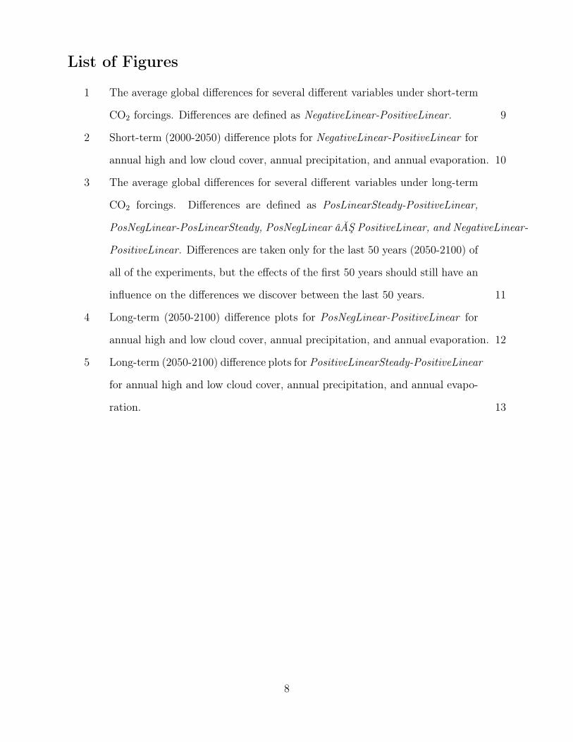
List of Figures
1 The average global differences for several different variables under short-term
CO2 forcings. Differences are defined as NegativeLinear-PositiveLinear. 9
2 Short-term (2000-2050) difference plots for NegativeLinear-PositiveLinear for
annual high and low cloud cover, annual precipitation, and annual evaporation. 10
3 The average global differences for several different variables under long-term
CO2 forcings. Differences are defined as PosLinearSteady-PositiveLinear,
PosNegLinear-PosLinearSteady, PosNegLinear âĂŞ PositiveLinear, and NegativeLinear-
PositiveLinear. Differences are taken only for the last 50 years (2050-2100) of
all of the experiments, but the effects of the first 50 years should still have an
influence on the differences we discover between the last 50 years. 11
4 Long-term (2050-2100) difference plots for PosNegLinear-PositiveLinear for
annual high and low cloud cover, annual precipitation, and annual evaporation. 12
5 Long-term (2050-2100) difference plots for PositiveLinearSteady-PositiveLinear
for annual high and low cloud cover, annual precipitation, and annual evapo-
ration. 13
8
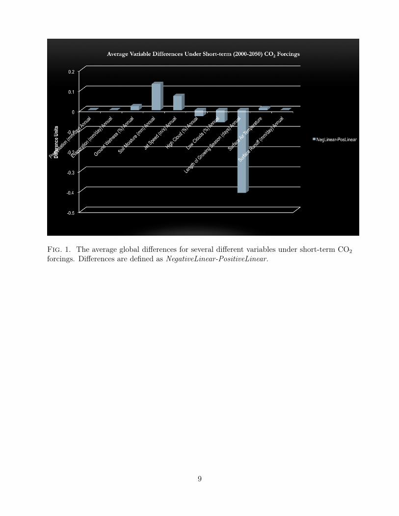
Fig. 1. The average global differences for several different variables under short-term CO2
forcings. Differences are defined as NegativeLinear-PositiveLinear.
9
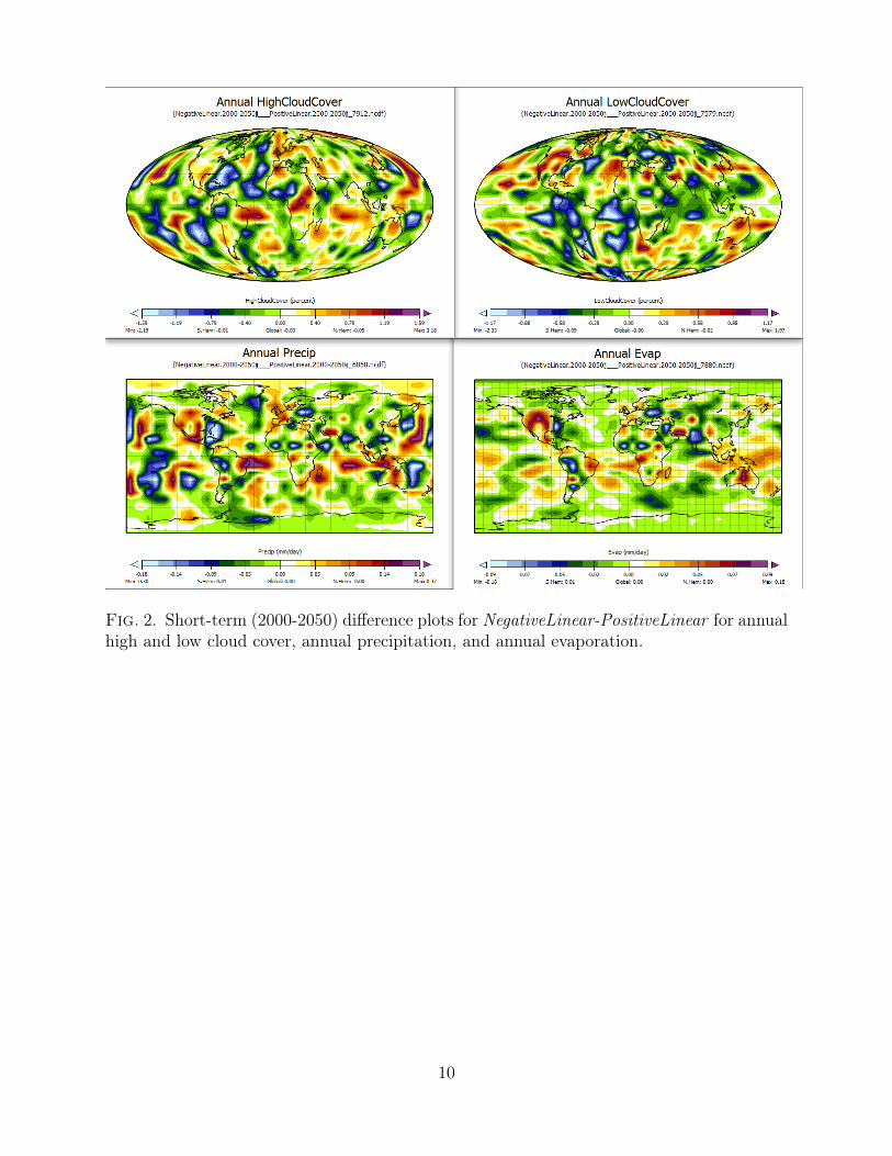
Fig. 2. Short-term (2000-2050) difference plots for NegativeLinear-PositiveLinear for annualhigh and low cloud cover, annual precipitation, and annual evaporation.
10
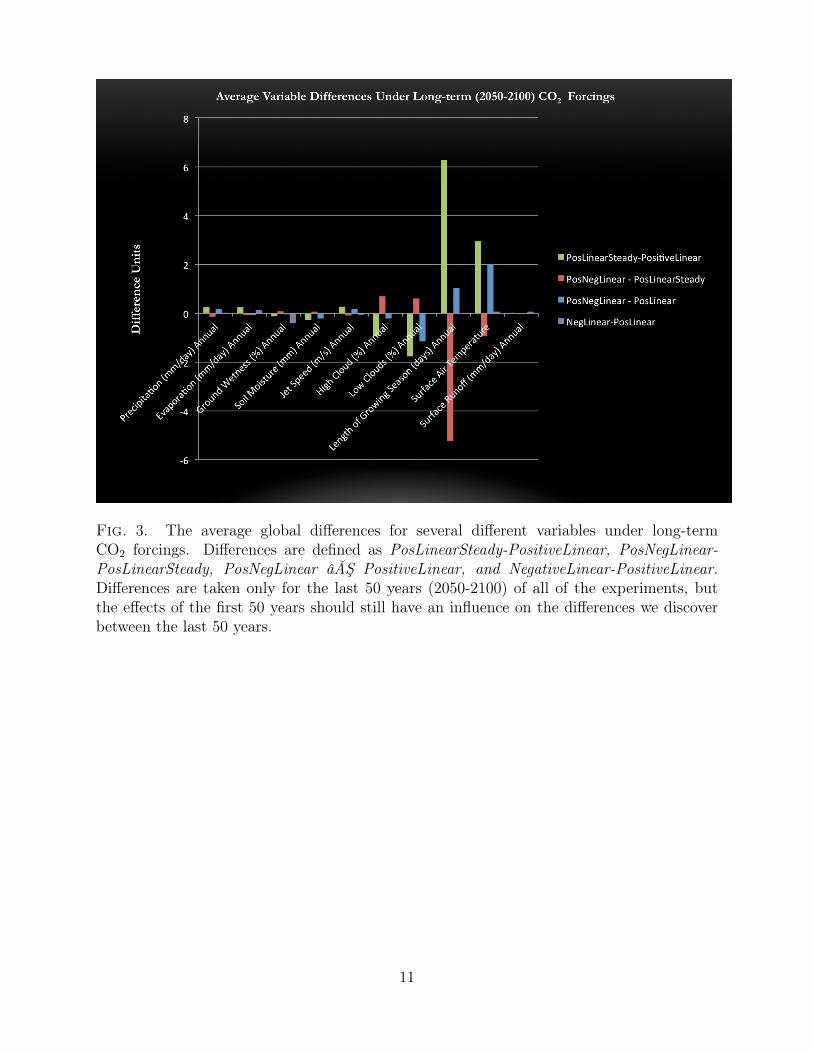
Fig. 3. The average global differences for several different variables under long-termCO2 forcings. Differences are defined as PosLinearSteady-PositiveLinear, PosNegLinear-PosLinearSteady, PosNegLinear âĂŞ PositiveLinear, and NegativeLinear-PositiveLinear.Differences are taken only for the last 50 years (2050-2100) of all of the experiments, butthe effects of the first 50 years should still have an influence on the differences we discoverbetween the last 50 years.
11
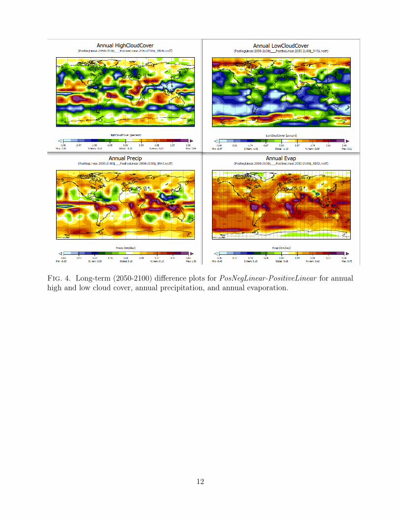
Fig. 4. Long-term (2050-2100) difference plots for PosNegLinear-PositiveLinear for annualhigh and low cloud cover, annual precipitation, and annual evaporation.
12
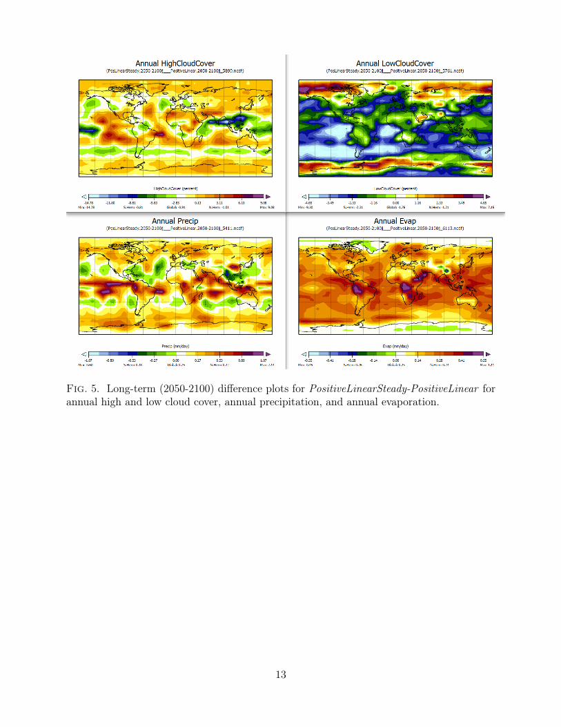
Fig. 5. Long-term (2050-2100) difference plots for PositiveLinearSteady-PositiveLinear forannual high and low cloud cover, annual precipitation, and annual evaporation.
13


