53
Edge Detection EE/CSE 576 Linda Shapiro

Edge Detection
EE/CSE 576 Linda Shapiro

Edge
Attneave's Cat (1954)
2

Edges are caused by a variety of factors.
depth discontinuity
surface color discontinuity
illumination discontinuity
surface normal discontinuity
Origin of edges

Characterizing edges • An edge is a place of rapid change in the
image intensity function
image intensity function
(along horizontal scanline) first derivative
edges correspond to extrema of derivative
4

• The gradient of an image:
• The gradient points in the direction of most rapid change in intensity
Image gradient
5
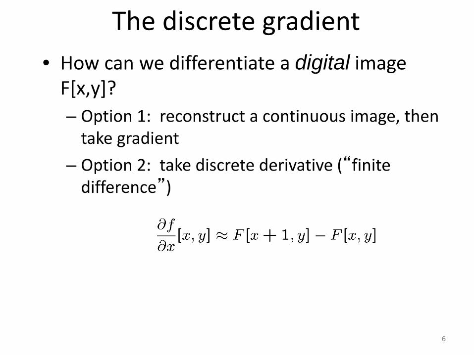
The discrete gradient • How can we differentiate a digital image
F[x,y]? – Option 1: reconstruct a continuous image, then
take gradient – Option 2: take discrete derivative (“finite
difference”)
6

The gradient direction is given by:
How does this relate to the direction of the edge? The edge strength is given by the gradient magnitude
Simple image gradient
How would you implement this as a filter?
7
perpendicular
or various simplifications
0 -1 1

Sobel operator
-1 0 1
-2 0 2
-1 0 1
-1 -2 -1
0 0 0
1 2 1
Magnitude:
Orientation:
In practice, it is common to use:
What’s the C/C++ function? Use atan2
Who was Sobel?

Sobel operator
Original Orientation Magnitude

Effects of noise • Consider a single row or column of the image
– Plotting intensity as a function of position gives a signal
Where is the edge? 10

Effects of noise
• Difference filters respond strongly to noise – Image noise results in pixels that look very
different from their neighbors – Generally, the larger the noise the stronger the
response
• What can we do about it?
Source: D. Forsyth 11

Where is the edge?
Solution: smooth first
Look for peaks in 12

• Differentiation is convolution, and convolution is associative:
• This saves us one operation:
gdxdfgf
dxd
∗=∗ )(
Derivative theorem of convolution
gdxdf ∗
f
gdxd
Source: S. Seitz How can we find (local) maxima of a function? 13
We don’t do that.

Remember: Derivative of Gaussian filter
x-direction y-direction
14

Laplacian of Gaussian • Consider
Laplacian of Gaussian operator
Where is the edge? Zero-crossings of bottom graph 15

2D edge detection filters
is the Laplacian operator:
Laplacian of Gaussian
Gaussian derivative of Gaussian
16

Edge detection by subtraction
original 17

Edge detection by subtraction
smoothed (5x5 Gaussian) 18

Edge detection by subtraction
smoothed – original (scaled by 4, offset +128)
19

Using the LoG Function (Laplacian of Gaussian)
• The LoG function will be – Zero far away from the edge – Positive on one side – Negative on the other side – Zero just at the edge
• It has simple digital mask implementation(s) • So it can be used as an edge operator • BUT, THERE’S SOMETHING BETTER
20

Canny edge detector
• This is probably the most widely used edge detector in computer vision
J. Canny, A Computational Approach To Edge Detection, IEEE Trans. Pattern Analysis and Machine Intelligence, 8:679-714, 1986.
Source: L. Fei-Fei 21

The Canny edge detector
• original image (Lena) 22
Note: I hate the Lena images.

The Canny edge detector
norm of the gradient
23

The Canny edge detector
thresholding
24

Get Orientation at Each Pixel
theta = atan2(-gy, gx)
25

The Canny edge detector
26

The Canny edge detector
thinning (non-maximum suppression)
27
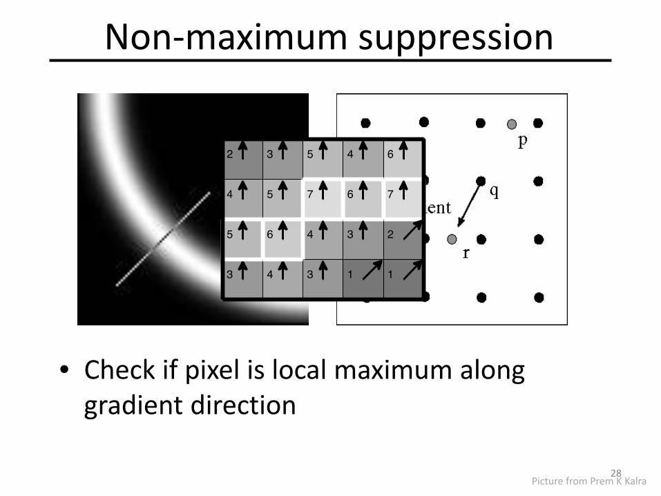
Non-maximum suppression
• Check if pixel is local maximum along gradient direction
Picture from Prem K Kalra 28

Canny Edges
30

Canny on Kidney
31

Canny Characteristics
• The Canny operator gives single-pixel-wide images with good continuation between adjacent pixels
• It is the most widely used edge operator today; no one has done better since it came out in the late 80s. Many implementations are available.
• It is very sensitive to its parameters, which need to be adjusted for different application domains.
32

Effect of σ (Gaussian kernel spread/size)
Canny with Canny with original
The choice of depends on desired behavior • large detects large scale edges • small detects fine features
33

An edge is not a line...
How can we detect lines ?
34

Finding lines in an image
• Option 1: – Search for the line at every possible
position/orientation – What is the cost of this operation?
• Option 2: – Use a voting scheme: Hough transform
35

• Connection between image (x,y) and Hough (m,b) spaces – A line in the image corresponds to a point in Hough
space – To go from image space to Hough space:
• given a set of points (x,y), find all (m,b) such that y = mx + b
x
y
m
b
m0
b0
image space Hough space
Finding lines in an image
36

Hough transform algorithm • Typically use a different parameterization
– d is the perpendicular distance from the line to the
origin – θ is the angle of this perpendicular with the
horizontal.
37

Hough transform algorithm • Basic Hough transform algorithm
1. Initialize H[d, θ]=0 2. for each edge point I[x,y] in the image
for θ = 0 to 180
H[d, θ] += 1
3. Find the value(s) of (d, θ) where H[d, θ] is maximum 4. The detected line in the image is given by
• What’s the running time (measured in # votes)?
38
1. How big is the array H? 2. Do we need to try all θ?
d
θ
Array H

Example
0 0 0 100 100 0 0 0 100 100 0 0 0 100 100 100 100 100 100 100 100 100 100 100 100
- - 0 0 - - - 0 0 - 90 90 40 20 - 90 90 90 40 - - - - - -
- - 3 3 - - - 3 3 - 3 3 3 3 - 3 3 3 3 - - - - - -
360 . 6 3 0
- - - - - - - - - - - - - - - - - - - - - 4 - 1 - 2 - 5 - - - - - - -
0 10 20 30 40 …90
360 . 6 3 0
- - - - - - - - - - - - - - - - - - - - - * - * - * - * - - - - - - -
(1,3)(1,4)(2,3)(2,4)
(3,1) (3,2) (4,1) (4,2) (4,3)
gray-tone image DQ THETAQ
Accumulator H PTLIST
distance angle
39

Chalmers University of Technology
40

Chalmers University of Technology
41

How do you extract the line segments from the accumulators?
pick the bin of H with highest value V while V > value_threshold { • order the corresponding pointlist from PTLIST • merge in high gradient neighbors within 10 degrees • create line segment from final point list • zero out that bin of H • pick the bin of H with highest value V }
42

Line segments from Hough Transform
43

Extensions • Extension 1: Use the image gradient
1. same 2. for each edge point I[x,y] in the image
compute unique (d, θ) based on image gradient at (x,y) H[d, θ] += 1
3. same 4. same
• What’s the running time measured in votes?
• Extension 2 – give more votes for stronger edges
• Extension 3 – change the sampling of (d, θ) to give more/less resolution
• Extension 4 – The same procedure can be used with circles, squares, or any other shape,
How? • Extension 5; the Burns procedure. Uses only angle, two different
quantifications, and connected components with votes for larger one.
44

A Nice Hough Variant The Burns Line Finder
1. Compute gradient magnitude and direction at each pixel. 2. For high gradient magnitude points, assign direction labels to two symbolic images for two different quantizations. 3. Find connected components of each symbolic image.
1 2 3
4 5
6 7 8 1
2 3 4 5 6 7 8
• Each pixel belongs to 2 components, one for each symbolic image.
• Each pixel votes for its longer component.
• Each component receives a count of pixels who voted for it.
• The components that receive majority support are selected.
-22.5
+22.5 0
45
45

Example
46
Quantization 1 Quantization 2
• Quantization 1 leads to 2 yellow components and 2 green. • Quantization 2 leads to 1 BIG red component. • All the pixels on the line vote for their Quantization 2 component. It becomes the basis for the line.
1 2 3
4 5
6 7 8 1
2 3 4 5 6 7 8 -22.5
+22.5 0

Burns Example 1
47

Burns Example 2
48

Hough Transform for Finding Circles
Equations: r = r0 + d sin θ c = c0 - d cos θ
r, c, d are parameters
Main idea: The gradient vector at an edge pixel points to the center of the circle.
*(r,c) d
49

Why it works
Filled Circle: Outer points of circle have gradient direction pointing to center.
Circular Ring: Outer points gradient towards center. Inner points gradient away from center.
The points in the away direction don’t accumulate in one bin!
50

51
Procedure to Accumulate Circles
• Set accumulator array A to all zero. Set point list array PTLIST to all NIL. • For each pixel (R,C) in the image { For each possible value of D { - compute gradient magnitude GMAG - if GMAG > gradient_threshold { . Compute THETA(R,C,D) . R0 := R - D*sin(THETA) . C0 := C + D*cos(THETA) . increment A(R0,C0,D) . update PTLIST(R0,C0,D) }}

52

Finding lung nodules (Kimme & Ballard)
53

Finale
• Edge operators are based on estimating derivatives. • While first derivatives show approximately where the
edges are, zero crossings of second derivatives were shown to be better.
• Ignoring that entirely, Canny developed his own edge detector that everyone uses now.
• After finding good edges, we have to group them into lines, circles, curves, etc. to use further.
• The Hough transform for circles works well, but for lines the performance can be poor. The Burns operator or some tracking operators (old ORT pkg) work better.
54


