IPA97 SPECIA L SECTION Edge operator error estimation incorporating measurements of CCD TV camera translferfunction R.C.Staunton Indexing terms: Transferfunction, CCD camera, Image sampling, Edge detector accuracy Abstract: A method for measuring the two- dimensional modulation transfer function of an image acquisition system with a CCD TV camera input device is presented. The measurements are then used in the estimation of image edge operator performance. A high resolution edge profile is assembled after the analysis of many profiles from the image of a step. Modulation transfer function measurements beyond the system’s Nyquist limit have been obtained. A minimum of apparatus is required. The performances of several systems have been compared. The band limiting of spatial frequencies are considered with respect to signal aliasing, matching components, feature representation and image operator accuracy. The results indicate the efficiency of system aliasing and reconstruction filters, differences in the vertical and horizontal responses of CCD arrays, and that the rectangular CCD element shape has not deflected the shape of the two dimensional modulation transfer function. Various edge operators have been tested and compared using high resolution edge spread function data computed during the transfer function measurements. These data were from realistically smoothed edges and represent the most difficult edges that the practical system would need to detect. Significant differences were found between results using the traditional pixel average and the new step edge models, indicating that in some cases a simpler, more computationally efficient operator may be sufficient. 1 Introduction Many of the analogue front end components of a dig- ital image processing system low-pass filter the light or electronic signals they process. The lens of a camera and its charge coupled device (CCD) array can be con- sidered as two-dimensional (2-D) filters, whereas the camera electronics and the digitiser’s antialiasing filter can be considered to be one-dimensional (1 -D). This 0 IEE, 1998 Paper first received 12th December 1997 and in remsed form 28th April 1998 The author is with the Department of Engneenng, Umversity of War- wck, Coventry CV4 7AL, UK IEE P~oceedznp onhe no 19981915 IEE Proc.-Vis. Image Signal Process., Vol. 145, No. 3, June 1998 paper describes a method by which the combined effect of these components, the front eind modulation transfer function (MTF), can be measured and discusses the implications of this band limiting for image processing. Measurements of the optical transfer function (OTF), which contains both gain and phase information, and the MTF, which is the modulus of the OTF, have been used extensively for evaluating lenses and continuous systems such as film cameras [I, 21. These traditional techniques fail with TV cameras and imagers contain- ing discrete devices, such as CCD arrays or analogue- to-digital converters (ADC), due to signal aliasing. Sig- nal aliasing results from the foldiing back of frequencies above the Nyquist limit to frequencies below it. In a typical TV camera based acquisition system continuous signals from the object are focused onto the surface of the CCD array by the lens, which also band-limits their spatial frequencies. Often significant signal components above the Nyquist frequency of the array are unchanged by the lens [l]. The CCD array elements integrate the image over i.heir active area and for a set exposure time. This information is held as an electric charge. This integration can also be considered as low- pass filtering, but again is insufficient to prevent alias- ing [2]. The charges stored in the array are then raster scanned using charge shifting mechanisms [3] and con- verted to electronic signals that can be further proc- essed by, for instance, a horizontal reconstruction filter. For a typical system, the input to the frame grabber is vertically discrete and horizontallly continuous. The ras- tered signal is then sampled at the ADC. If the sam- pling frequency of the AlDC is appropriate, the image can be considered as sarnpled on a square grid. The accurate representation of the object by the sampled image is a function of the quality of the acquisition sys- tem. The MTF can be measured by a knife edge technique [I]. Light from a suitably long and straight step edge object is focused by the camera lens onto the CCD array, a TV frame is grabbed, aind the MTF is calcu- lated. Problems occur with discrete system measure- ments as, ideally, the akerage response of the entire CCD array and its frequency response beyond the Nyquist limit are required. Reichenbach et al. [2] have reported a knife edge technique for use with discrete systems where the edge is used to provide many step profiles in the digitised image that can be assembled to produce a composite, (ESF) that contains non-aliased spatial frequency infor- mation obtained from several elements in the CCD array. The ESFs were obtained for vertical and hor- izontal edges and were then further processed by a low noise, high resoltitiam 1-D edge spread function 229
Transcript
IPA97 SPECIA L SECTION
Edge operator error estimation incorporating measurements of CCD TV camera translfer function
Abstract: A method for measuring the two- dimensional modulation transfer function of an image acquisition system with a CCD TV camera input device is presented. The measurements are then used in the estimation of image edge operator performance. A high resolution edge profile is assembled after the analysis of many profiles from the image of a step. Modulation transfer function measurements beyond the system’s Nyquist limit have been obtained. A minimum of apparatus is required. The performances of several systems have been compared. The band limiting of spatial frequencies are considered with respect to signal aliasing, matching components, feature representation and image operator accuracy. The results indicate the efficiency of system aliasing and reconstruction filters, differences in the vertical and horizontal responses of CCD arrays, and that the rectangular CCD element shape has not deflected the shape of the two dimensional modulation transfer function. Various edge operators have been tested and compared using high resolution edge spread function data computed during the transfer function measurements. These data were from realistically smoothed edges and represent the most difficult edges that the practical system would need to detect. Significant differences were found between results using the traditional pixel average and the new step edge models, indicating that in some cases a simpler, more computationally efficient operator may be sufficient.
1 Introduction
Many of the analogue front end components of a dig- ital image processing system low-pass filter the light or electronic signals they process. The lens of a camera and its charge coupled device (CCD) array can be con- sidered as two-dimensional (2-D) filters, whereas the camera electronics and the digitiser’s antialiasing filter can be considered to be one-dimensional (1 -D). This 0 IEE, 1998
Paper first received 12th December 1997 and in remsed form 28th April 1998 The author is with the Department of Engneenng, Umversity of War- wck, Coventry CV4 7AL, UK
IEE P~oceedznp o n h e no 19981915
IEE Proc.-Vis. Image Signal Process., Vol. 145, No. 3, June 1998
paper describes a method by which the combined effect of these components, the front eind modulation transfer function (MTF), can be measured and discusses the implications of this band limiting for image processing.
Measurements of the optical transfer function (OTF), which contains both gain and phase information, and the MTF, which is the modulus of the OTF, have been used extensively for evaluating lenses and continuous systems such as film cameras [ I , 21. These traditional techniques fail with TV cameras and imagers contain- ing discrete devices, such as CCD arrays or analogue- to-digital converters (ADC), due to signal aliasing. Sig- nal aliasing results from the foldiing back of frequencies above the Nyquist limit to frequencies below it. In a typical TV camera based acquisition system continuous signals from the object are focused onto the surface of the CCD array by the lens, which also band-limits their spatial frequencies. Often significant signal components above the Nyquist frequency of the array are unchanged by the lens [l]. The CCD array elements integrate the image over i.heir active area and for a set exposure time. This information is held as an electric charge. This integration can also be considered as low- pass filtering, but again is insufficient to prevent alias- ing [2]. The charges stored in the array are then raster scanned using charge shifting mechanisms [3] and con- verted to electronic signals that can be further proc- essed by, for instance, a horizontal reconstruction filter. For a typical system, the input to the frame grabber is vertically discrete and horizontallly continuous. The ras- tered signal is then sampled at the ADC. If the sam- pling frequency of the AlDC is appropriate, the image can be considered as sarnpled on a square grid. The accurate representation of the object by the sampled image is a function of the quality of the acquisition sys- tem.
The MTF can be measured by a knife edge technique [I]. Light from a suitably long and straight step edge object is focused by the camera lens onto the CCD array, a TV frame is grabbed, aind the MTF is calcu- lated. Problems occur with discrete system measure- ments as, ideally, the akerage response of the entire CCD array and its frequency response beyond the Nyquist limit are required.
Reichenbach et al. [2] have reported a knife edge technique for use with discrete systems where the edge is used to provide many step profiles in the digitised image that can be assembled to produce a composite,
(ESF) that contains non-aliased spatial frequency infor- mation obtained from several elements in the CCD array. The ESFs were obtained for vertical and hor- izontal edges and were then further processed by a
low noise, high resoltitiam 1-D edge spread function
229
Fourier domain technique to give the MTF. Their method utilised the discrete Fourier transform and required periodically extended data from multiple knife edges. Tzannes and Mooney [4] improved the technique by employing a spatial domain approach requiring only a single edge.
In this paper, the above method is extended to enable measurements to be made for edges presented at any angle to the camera. Measurements in 2-D of both the ESF and MTF of three raster scanned TV cameras and two frame grabber systems have been compared. In each case the resulting images had resolutions of 512 x 512 pixels. The measurements, although performed in the laboratory, required only the simple apparatus of a knife edge and a direct current (DC) light box.
To obtain the high resolution ESF with this tech- nique, edge profiles across the discrete image of the knife edge are modelled and then registered with each other, assuming the edge to be straight. Because of this registering, geometric image distortions caused by the lens or the camera are not detectable. Barrel distortion, in which the image of a straight line located away from the centre of the image becomes curved, is one example of geometric distortion. The resultant MTFs are unlikely to be useful for image restoration. Another limitation is that the system's response must be linear. This requires the camera's automatic gain control (AGC) and gamma correction to be disabled, thus measurements are most useful in controlled lighting and machine vision applications. A non-parametric technique which overcomes problems with geometric and amplitude distortion in the measurement of the point spread function (PSF) and its application to a thermal image flying spot scanner has recently been published [5] .
The MTF method used here is easy to apply and has been designed to work on a computing platform with a C compiler and the standard Matlab package. The 2-D MTF can be used to investigate the production of ali- ased components when the image is sampled by the CCD array, and a horizontal l-D MTF used to investi- gate the band limiting characteristics of the input sec- tion of the frame grabber. The 2-D MTF has implications for the efficient sampling of the image [6] and to system spatial resolution, in that a feature dis- tinguished when presented at one angle may be missed at another, or measurements may potentially be more accurate on a feature presented at one angle than at another. The main application presented here concerns measurements of the gradient and angle accuracy of edge operators.
Traditionally, edge operators have been tested on step edges as these have been considered the most diffi- cult edges to detect accurately [7]. These edges have been synthesised within a computer and modified to allow for pixel shaped windowing of the data while sampling [SI. In this paper, realistic physical models based on the ESF measurements are used for testing the operators and the results compared with those from the pixel window approach. The high resolution 1-D ESF can be considered as being copied vertically through a 2-D space to produce a high resolution image of an edge in which the line joining the points of inflection of the ESFs align vertically and pass through the centre of the image. Such a 2-D image is shown in Fig. 1. A sampling grid with the correct resolution and number of points with which to test an edge detector
230
are then applied at random position and orientation with respect to the edge, and the image is resampled to provide test data. In this way accuracy statistics can be compiled.
X
high brightness low brightness Fig. 1 pled (Xi by run&mly translated and oriented 3 x 3 grid
ESF CO ied vertically to form high resolution 2-D image and sum-
2 Camera and frame grabber specifications
The following specifications have been obtained from the manufacturers' data sheets: Camera A: 213 inch CCD. Square shaped element area. Horizontal and vertical sampling point spacing 10 prn. Resolution: 756 elements horizontal x 58 1 vertical. Lens: Fixed focal length, 16". AGC select switch. Gamma correction factory set to 1.0. Cameva B: 1/2 inch CCD. Resolution: 752 elements horizontal x 582 vertical. Lens: Fixed focal length, 16". AGC select switch. Gamma correction switcha- ble to 0.45 or 1.0. Camera C: 113 inch CCD. Resolution: 750 elements horizontal. Vertical resolution not stated. Lens: Fixed focal length, 16". AGC select switch. Gamma cor- rection switchable: On or Off. Frame grubber X: 512 x 512 pixels. Aspect ratio: 1 to 1. Frame grubber Y: 512 x 512 pixels. Aspect ratio: 4 to 3.
3 Measurement of 2-D MTF
The first step is to set up the camera to be as linear as possible. The AGC should be disabled and the gamma correction removed. A high resolution ESF is then assembled from several low resolution ESFs. Knife edge methods that assemble a high resolution l-D ESF from the contributions of low resolution ESFs along the edge have been reported in the literature [2, 4, 9, 101. If the image of the edge does not align with an axis of symmetry of the CCD array, sampling points along a profile at right angles to the edge will be positioned differently with respect to the edge discontinuity as it is moved along the edge. For a 512 x 512 CCD array it can easily be arranged for at least 512 elements to be cut by the edge, and for at least 512 profiles to be measured from which the high resolution ESF can be assembled. Commercial systems are available that mechanically increment the position of an edge to effect the same result, but here we are researching a method with a greater potential for application outside
IEE Proc.-Vis. Image Signal Process., Vol. 145, No. 3, June 1998
the laboratory and that includes the limitations of the frame grabber. The ESF provides data on which edge detectors can be tested [9, lo], but for general use the ESF can be differentiated and transformed to the Fou- rier plane to give the OTF.
'h 0.8
0.6
0.4
0.2
0 0 0.5 1 1.5 2 2.5 3
normalised frequency f/fNyq a
250 i 2oo t 7
0 -10 -8 -6 -4 -2 0 2 4 6 8 10
CCD element spacing
b Fig.2 a Typical MTF b Typical ESF
Camera A, frame grabber X
The knife edge was a straight edge mounted on a DC light box at a known angle to the base of the camera and at a distance of 0.5m from the front of the lens. Light from the edge was the acquisition system's input and the image data in the frame store, its output. An optical filter was used to block infrared (IR) from entering the lenses. Cameras A and B with their lens combinations were found to be IR sensitive in that a slightly lower cut-off frequency was measured when imaging the DC light box directly than when the IR was blocked. The processing was implemented using a combination of C and Matlab, and was based on the 1-D method developed by Tzannes and Mooney [4]. However, cubic splines were fitted to the ESF instead of Fermi functions before differentiation to obtain the point spread function (PSF). Cubic spline functions are readily available in the Matlab package and formed a good fit to all the edge profiles processed. The modulus of the Fourier transform of the PSF gives the MTF of the system. Fig. 2 shows simulated and measured 1-D MTFs and an ESF for an acquisition system compris- ing camera A and frame grabber X. The simulation result is obtained by modelling the diffraction limit of
IEE Proc.-Vis. Image Signal Process., Vol. 145, No. 3, June 1998
the lens and a rectangular reception profile for a CCD element [4]. Lens aberrations [I], light reflection and charge leakage within the CCD array [ll], and low- pass filters within the frame grabber or the camera's electronics, will also liniit the high frequency response and may explain the differences between the simulated and actual results.
The basic method was designed for edges presented to the camera at 0 or 910 degrees and had to be modi- fied to enable data at other angles to be processed for the compilation of a 2-D MTF. First, the edge angle was measured to an accuracy of k0.65 degrees using a 7 x 7 integrated directiional derivative detector (IDD) [12] and averaging over all edge pixels to obtain a high signal-to-noise ratio (SIVR). The angle of a normal to the edge can then be found. To obtain a low resolution ESF, brightness samples on a normal to the edge are extracted into a 1-D array. Samples on edge normals are readily obtained for edge angles of 0 or 90 degrees as each normal can be chosen to pass directly through a number of image sampling points. At other angles it is possible to lock a noirmal to a single sampling point, but a closely spaced sequence of samples across the edge is required. As shown in Fig. 3, for these angles a 1-D shift parallel to the edge was performed from nearby grid points to estimate brightness values on these normals. This simple technique was sufficient as brightness contours were found to be reasonably paral- lel to the edge. These brightness values were usually not equally spaced along the normal, but more were obtained per unit distaince than for the 0 or 90 degree edges, increasing the resolution of the ESF.
? grid point I
Fig. 3 sition of brightness data along the normal
Edge and normal positions within square sumpling grid and acqui-
1
0.8
.- 5 - ';j
E!
,E P
0.6
U 3 0.4
0.2
0 0 0.5 1 1.5
spatial frequency nornialised to Nyquist frequency of CCD array I-D MTFs obtained from ed!e normals at angles of 0 to 90 Fig.4
degrees to the horizontal for camera A, frame grabber X
23 1
For the 2-D MTF results presented here, 1-D MTFs were computed for the quadrant 0 to 90 degrees in 15 degree steps. Fig. 4 shows the seven I-D MTFs obtained when camera A was connected to frame Grabber X. The 0 degree MTF has the lowest cut-off frequency, with the cut-off frequency of the others increasing as the angle of the edge normal at which the MTF was obtained increases. This reduction in cut-off frequency at lower normal angles could be a result of either a low-pass filter in the camera’s analogue output circuitry or an anti-aliasing filter in the frame grabber. Each would operate maximally in the horizontal (0 degree) direction.
Fig. 5 shows polar plots of the -3dB modulation points of the 2-D MTFs obtained from various camera and frame grabber combinations. Each camera has a 512 x 512 CCD array, but the sampling point spacing varies between cameras. To enable a comparison between the frequency responses of the different sys- tems, they have been normalised to the vertical Nyquist frequency of camera A. For each camera system the vertical sampling point spacing was found to be within 1% when connected to frame grabber X or Y.
0.6
0.2
0 0 0.2 04 0.6 0.8
normalised frequency Fig.5 Polar obtainedfrom e&e normals at angles of0 to 90 degrees to the horizontal a Camera A, Grabber Y b Camera A, Grabber X c Camera B, Grabber Y d Camera B, Grabber X e Camera C, Grabber Y f Camera C, Grabber X
lots of the -3dB modulation paints of the 2-D MTFs
The vertical normalised cut-off frequencies for each test lie in the range 0.37 to 0.69, whereas the horizontal normalised cut-off frequencies lie in the range 0.27 to 0.48. Vertically, the lens and the CCD array are the main factors limiting the cut-off frequency. Horizon- tally, the camera and frame grabber electronics can also limit the cut-off frequency as they process the raster scanned signals. The different vertical and hori- zontal shifting processes within the CCD devices (inter- line transfer devices) that are used to effect the rastered output may also modify cut-off frequencies differently at each edge application angle.
The trace for camera A connected to grabber X shows an increase in cut-off frequency with an increase in the angle of the edge normal, whereas for camera B and grabber X the band limiting is more nearly circu- lar. For camera C connected to grabber X there is
232
again an increase in the cut-off frequency with increas- ing angle. The cut-off frequencies for the system combi- nations of camera A and camera C with grabber X are being limited maximally in the horizontal direction. Reconstruction or other filters in the camera’s electron- ics, and anti-aliasing filters in the grabber operate in the horizontal direction, but as the horizontal cut-off for the camera A system is so much lower than for the other systems, the limiting must be by filtering within the camera. If the grabbers have anti-aliasing filters then their cut-off frequencies must be close to the hori- zontal Nyquist frequencies of 1.00 for grabber X and 0.75 for grabber Y. There is evidence for such filtering as the measured horizontal cut-off frequencies for cam- eras B and C connected to grabber Y are lower than those for grabber X. The possibility of signal aliasing due to sampling by the grabber can be seen in Fig. 4. The horizontal frequency signals have been highly attenuated above the Nyquist frequency, although this is by the camera’s electronics which process the raster scanned lines, whereas the normalised modulation of the vertical signals are above 0.2 at this frequency.
If the only frequency limitation was due to the rec- tangular CCD elements then the frequency plane would be tiled by periodically extended rectangular band regions [6], which, given an optimal 2-D anti-aliasing filter, would reduce to a single rectangular band region. In which case the highest frequency in each trace on the polar plot would be at 45 degrees (grabber X) or 60 degrees (grabber Y). For these practical measurements no increase at these frequencies was observed, indicat- ing that the CCD elements were either not rectangular, or not integrating light energy uniformly throughout their area, that there was charge leakage or light scat- tering within the device, or that other system elements were smoothing the signals. Lens diffraction limiting will circularly band limit in the frequency plane and therefore would limit the frequency of the 45 or 60 degree MTFs equally with that at other frequencies.
4 Operator performance
By convolving a model of an object to be displayed with the OTF and adding noise, a digitised image as it would be degraded by the imaging system can be obtained on which to test a recognition or measure- ment process. As an example edge detection is consid- ered further.
4. I Edge model Lyvers and Mitchell [8] and Haralick and Shapiro [12] have used edge models that incorporate pixel averaging to compare the accuracy of several edge detectors rang- ing in size from 3 x 3 to 7 x 7 pixels. Their edges were a function of edge orientation, edge position within the central pixel, edge contrast and a rectangular pixel area. Sampled values were the average brightness in the pixel window. Such pixel averaging could be considered to incorporate a simple model of a rectangular CCD sensing element. However, as noted in Section 3, for the cameras tested there was no deflection in the MTFs to indicate that a rectangular shaped element would affect the system model. The ESF provides a more real- istic edge model and, in addition, can be used more efficiently. The edge model used here was obtained from the 1-D ESF by combining the results from sev- eral CCD elements. It is reasonably noise free and can easily be translated and re-sampled to produce a high
IEE Proc -VIS Imuge Signal Pvocess , Vol 145, No 3, June 1998
resolution 2-D image of a vertical edge with its half height points positioned half way across. A grid of sampling points can then be positioned at random translations and angles with respect to the edge to pro- duce sets of image data on which to test an edge detec- tor. Gaussian distributed random noise can be added to the sampled values. The signal-to-noise ratio is defined as
(3 dB S N R = 2010g,,
where c is the edge contrast [13] and CJ the standard deviation of the noise. Once the ESF is known, the technique has a greater computational efficiency than the pixel averaging technique, in that thousands of ran- dom edges could be tested in seconds rather than min- utes (Sun Ultra 140).
4.2 Edge detector error estimation Errors will occur in position, height, gradient and angle measurements. The high resolution edge simulated from the ESF contains an edge, the position of which is typically known to within *0.2% of the re-sampling grid point spacing. The edge angle accuracy is similarly high and the height and gradient are realistic values. In this study, pairs of first derivative detectors were used which returned horizontal and vertical gradient vectors. These were analysed in the usual way to provide edge gradient and angle information. Such detectors exhibit larger errors with step edges than with planar edges [7], and the 2-D MTF results from Section 3 were con- sulted to find the most suitable ESF, the sharpest, on which to test the detectors. The detector templates tested varied in size from 3 x 3 to 7 x 7 pixels. A larger template should have a higher noise immunity and pro- duce more accurate results, but may take longer to compute. The templates are described either by Haral- ick and Shapiro [I21 or by Davies [14]. Davies describes two templates for the circular 7 x 7 operator, one with a design radius, r = 2.915 pixels, and the other with r = 3.500 pixels. Both were tested.
The operators tested are named in Table 1. For each operator 10000 randomly oriented and positioned edges of height 28 brightness units were tested, and sta- tistics of the angle error and gradient measurement were compiled.
Under gradient, the first column is the SD when the mean of the edge gradients is normalised to 100, and the second is the mean. Under angle error, the first column is the standard devi- ation (SD) of the error, and the second is the peak error
Table 1 compares tlhe perlformance of each edge operator when operating on nloise free edges modelled using the ESF. For four operators the angle error results can be further compared with results from tradi- tionally modelled edges published in [8]. Such compari- son shows the peak anglle errors with the ESF modelled edges to be approximately 50% of those from the tradi- tionally modelled edges. The smaller errors from the more realistic ESF model indicate that a smaller, more computationally efficient operator may be sufficient for a particular application. The gradient measurements were made on edges with a height matching the full range of the 8 bit digitisers. This has resulted in a wide spread of gradient values and differing mean gradient values for each detector. To enable easy comparison, the mean gradient of each detector has been shifted to 100 and a normalised SD calculated. The circular oper- ator gave the best gradient estimation and the IDD the best angle estimation for the grloup of 5 x 5 detectors in this noise free comparison. The circular 7 x 7 (v = 3.500) gave the best overall results.
Fig. 6 shows a compairison of the gradient estimation performance of each operator in the presence of noise. The 5 x 5 circular and 7 x 7 circular ( r = 3.500) opera- tors have performed best in their classes, although at low SNRs the distinctioiis are less clear. The mean and SD of the gradient can be used to influence the choice of threshold value for edge detector applications.
signal to noise ratio,dB Fig.6 a Sobel 3 x 3 b Sobel 5 x 5 c Prewitt 5 x 5 d Standard cubic facet 5 x 5 e Integrated directional derivative (IDD) 5 x 5 f Circular 5 x 5 P IDD 7 x 7
ESfect of noise on standard deviaiion of gradient estimation
" ~~
h Circular 7 x 7 (2.915) i Circular 7 x 7 (3.500) Edge contrast = 255 units. For standard deviations of gradient each mean value is scaled to 100
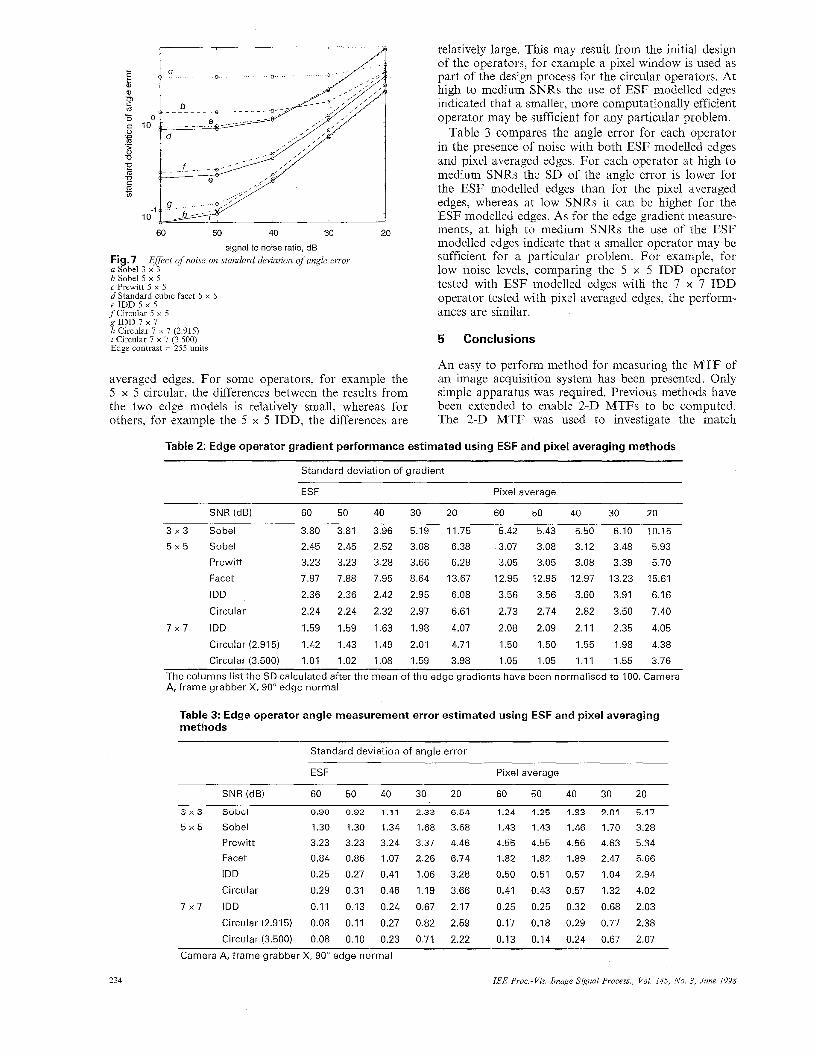
Fig. 7 shows a comparison of the angle error per- formance of each operalor in the presence of noise. The 5 x 5 IDD was the best 5 x 5 operator, and the 7 x 7 (v = 3.500) circular the best 7 x 7 operator. The 3 x 3 Sobel performed well at low noise levels, outperforming two of the 5 x 5 detectors for angle measurement.
Table 2 compares the gradient performance of each operator in the presence of noise, first, with ESF mod- elled edges and, secondly, with pixel averaged edges. Apart from the Prewitt operator, lower SDs of gradient measurements were recorded with the ESF modelled edges indicating that, in general, the cut-off frequency of the smoothing filtering in the ESF modelling was lower and the edge more planar than that in the pixel
233 IEE Proc-Vis. Image Signal Process., Vol. 145. No. 3, June 1998
60 50 40 30 20
signal to noise ratio, dB Fig.7 a Sobel 3 x 3 b Sobel 5 x 5
Effect of noise on standard deviation of angle error
c Prewitt 5 x 5 d Standard cubic facet 5 x 5 e IDD 5 x 5 fCircuiar 5 x 5 g IDD 7 x 7 h Circular 7 x 7 (2.915) i Circular 7 x 7 (3.500) Edge contrast = 255 units
averaged edges. For some operators, for example the 5 x 5 circular, the differences between the results from the two edge models is relatively small, whereas for others, for example the 5 x 5 IDD, the differences are
relatively large. This may result from the initial design of the operators, for example a pixel window is used as part of the design process for the circular operators. At high to medium SNRs the use of ESF modelled edges indicated that a smaller, more computationally efficient operator may be sufficient for any particular problem.
Table 3 compares the angle error for each operator in the presence of noise with both ESF modelled edges and pixel averaged edges. For each operator at high to medium SNRs the SD of the angle error is lower for the ESF modelled edges than for the pixel averaged edges, whereas at low SNRs it can be higher for the ESF modelled edges. As for the edge gradient measure- ments, at high to medium SNRs the use of the ESF modelled edges indicate that a smaller operator may be sufficient for a particular problem. For example, for low noise levels, comparing the 5 x 5 IDD operator tested with ESF modelled edges with the 7 x 7 IDD operator tested with pixel averaged edges, the perform- ances are similar.
5 Conclusions
An easy to perform method for measuring the MTF of an image acquisition system has been presented. Only simple apparatus was required. Previous methods have been extended to enable 2-D MTFs to be computed. The 2-D MTF was used to investigate the match
Table 2: Edge operator gradient performance estimated using ESF and pixel averaging methods
The columns list the SD calculated after the mean of the edge gradients have been normalised to 100. Camera A, frame grabber X, 90" edge normal
Table 3: Edge operator angle measurement error estimated using ESF and pixel averaging methods
Standard deviation of angle error
ESF Pixel average
SNR (dB) 60 50 40 30 20 60 50 40 30 20
3 x 3 Sobel 0.90 0.92 1.11 2.33 6.54
5 x 5 Sobel 1.30 1.30 1.34 1.68 3.68
Prewitt 3.23 3.23 3.24 3.37 4.46
Facet 0.84 0.86 1.07 2.26 6.74
IDD 0.25 0.27 0.41 1.06 3.28
Circular 0.29 0.31 0.46 1.19 3.66
7 x 7 IDD 0.11 0.13 0.24 0.67 2.17
Circular (2.915) 0.08 0.11 0.27 0.82 2.59
Circular (3.500) 0.08 0.10 0.23 0.71 2.22
1.24 1.25 1.33 2.01 5.17
1.43 1.43 1.46 1.70 3.28 4.55 4.55 4.56 4.63 5.34
1.82 1.82 1.89 2.47 5.66
0.50 0.51 0.57 1.04 2.94
0.41 0.43 0.57 1.32 4.02
0.25 0.25 0.32 0.68 2.03
0.17 0.18 0.29 0.77 2.38
0.13 0.14 0.24 0.67 2.07
Camera A, frame grabber X, 90" edge normal
234 IEE Proc-Vis. Image Signal Process., Vol. 14.5, No. 3, June 1998
between cameras and frame grabbers, with a circular band limit indicating that a feature would be equally represented when presented at any angle to the system. A near circular band limit was found with one camera and frame grabber combination.
Three cameras and two frame grabbers were tested in five system combinations. The systems were investi- gated for possible signal aliasing and it was found such aliasing was likely to occur with each combination. The technique was able to show the existence of a recon- struction filter in one camera, differences between the vertical and horizontal responses of the CCD arrays, that the 2-D MTF shape was independent of the rec- tangular CCD element shape, and that there were dif- ferent low-pass cut-off frequencies for the analogue electronics in each frame grabber.
The method was used to provide high resolution test data that enabled edge detector accuracy to be deter- mined. The edges used in the testing were modelled as step edges that had been modified by the lens-camera- frame grabber system, and represented the most diffi- cult to detect edges that would be found in a practical situation.
The detector errors were found to be less than those measured by traditional methods that use a pixel aver- aging model. This indicated that for a particular appli- cation a smaller, more computationally efficient operator may be sufficient. Detector tests were com- puted more quickly on the ESF modelled edges than on the pixel averaged edges.
~
6
1
2
3
4
5
6
7
8
9
References
RAY, S.F.: ‘Applied photographic optics’ (Focal Press, London, UK, 1988) REICHENBACH, S.E., PARK, S.K., and NARAYAN- SWAMY, R.: ‘Characterizing digitall image acquisition devices’, Opt. Eng., 1991, 30, (2), pp. 170-177 BATCHELOR, B.G., HILL, D.A., and HODGSON, D.C.: ‘Automated visual inspection’ (IFS Publications Ltd, UK, 1985) TZANNES, A.P., and MOONEY, J.M.: ‘Measurement of the modulation transfer function of infrared cameras’, Opt. Eng.,
ZANDHUIS, J.A., PYCOCK, D.., QUIGLEY, S.F., and WEBB, P.W.: ‘Sub-pixel non-parametric PSF estimation for image enhancement’, IEE Proc., Vis. Zmuge Signal Process., 1997, 144, (5), pp. 285-292 MERSEREAU, R.M.: ‘The processing of hexagonally sampled two dimensional signals’, Proc. IEEE, 1979, 67, (6), pp. 930-949 DAVIS, L.S.: ‘A survey of edge detection techniques’, Comput. Graph. Image Process., 1975, 4, pp. 248-270 LYVERS, E.P., and MITCHELL, O.R.: ‘Precision edge contrast and orientation estimation’, IEEE Trans., 1988, PAMI-10, (6) ,
STAUNTON, R.C.: ‘Edge (detector error estimation incorporat- ing CCD camera limitations’. Proceedings of IEEE Norsig96 Sig- nal processing conference, Espoo, Finland, 1996, pp. 243-246
1995, 34, (6), pp. 1808-1817
pp. 927-937
10 STAUNTON, R.c.: TCD camera transfer function measurement and its implication for sampling and operator performance’. Pro- ceedings of IEE IPA97 hiage processing and its applications, Dublin, Ireland, 1997, pp. 5’76-580