Edinburgh Research Explorer

Automated analysis and benchmarking of GCMC simulationprograms in application to gas adsorption.

Citation for published version:Gowers, R, Hajiahmadi Farmahini, A, Friedrich, D & Sarkisov, L 2017, 'Automated analysis andbenchmarking of GCMC simulation programs in application to gas adsorption.', Molecular simulation.https://doi.org/10.1080/08927022.2017.1375492

Digital Object Identifier (DOI):10.1080/08927022.2017.1375492

Link:Link to publication record in Edinburgh Research Explorer

Document Version:Peer reviewed version

Published In:Molecular simulation

General rightsCopyright for the publications made accessible via the Edinburgh Research Explorer is retained by the author(s)and / or other copyright owners and it is a condition of accessing these publications that users recognise andabide by the legal requirements associated with these rights.

Take down policyThe University of Edinburgh has made every reasonable effort to ensure that Edinburgh Research Explorercontent complies with UK legislation. If you believe that the public display of this file breaches copyright pleasecontact openaccess@ed.ac.uk providing details, and we will remove access to the work immediately andinvestigate your claim.

Download date: 03. Jun. 2020

July 3, 2017 Molecular Simulation main

To appear in Molecular SimulationVol. 00, No. 00, Month 20XX, 1–22

Automated analysis and benchmarking of GCMC simulation programs in

application to gas adsorption.

Richard J. Gowersa∗ Amir H. Farmahinia, Daniel Friedrichb, and Lev Sarkisova∗

aInstitute for Materials and Processes, School of Engineering, The University of Edinburgh, UK;bInstitute for Energy Systems, School of Engineering, The University of Edinburgh, UK

(Received 00 Month 20XX; final version received 00 Month 20XX)

In this work we set out to evaluate the computational performance of several popular Monte Carlo sim-ulation programs, namely Cassandra, DL Monte, Music, Raspa and Towhee, in modelling gas adsorptionin crystalline materials. We focus on the reference case of CO2 adsorption in IRMOF-1 at 208K.

To critically assess their performance, we first establish some criteria which allow us to make thisassessment on a consistent basis. Specifically, the total computational time required for a program tocomplete a simulation of an adsorption point, consists of the time required for equilibration plus timerequired to generate a specific number of uncorrelated samples of the property of interest.

Our analysis shows that across different programs there is a wide difference in the statistical value ofa single MC step, however their computational performance is quite comparable. We further explore theuse of energy grids and energy bias techniques, as well as the efficiency of the parallel execution of thesimulations. The test cases developed are made openly available as a resource for the community, andcan be used for validation and as a template for further studies.

Keywords: benchmarking; Grand Canonical Monte Carlo; adsorption; computational performance;sampling

1. Introduction

Recent advances in synthesis of novel porous materials, such as Metal-Organic Frameworks (MOFs),Zeolitic Imidazolate Frameworks (ZIFs) and polymers with intrinsic microporosity (PIMs) have aprofound impact on the way we now approach design of technologies and applications based onthese materials. Indeed, it is not possible to test the thousands of already discovered MOFs, ZIFs,PIMs and related materials in the context of each potential application, while the best materialfor a particular purpose may exist among those not yet synthesised, but hypothetically possiblestructures within these classes. Hence the idea of computational screening of materials, the newstarting point of process design and optimisation, which aims to identify the best material or groupof materials for a particular application before the actual experimental effort is committed.

Broadly speaking, computational screening can be separated into two phases. The first phaseinvolves building a database of possible structures, both real and hypothetical. The modular natureof these new materials allows one to guess the structure of not yet synthesised materials, usinga systematic variation and assembly of the building blocks through what can be best describedas molecular Lego approaches. In the second phase, computational methods are used to assessthe key characteristics of the materials within the database, based on the performance metricsassociated with a particular application. Although in principle this strategy can be employed in

∗Corresponding author. Email: richard.gowers@ed.ac.uk∗Corresponding author. Email: lev.sarkisov@ed.ac.uk

July 3, 2017 Molecular Simulation main

the context of any application, the tunable porosity and surface area of MOFs and ZIFs makes themparticularly interesting for adsorption applications, such as methane storage and carbon capture,and this is what most of the recent screening studies have been focused on. Prominent examplesof this approach include studies from Snurr and co-workers [1], Smit and co-workers [2] and Sholland co-workers [3]. For comprehensive reviews in the field of molecular simulation of adsorptionprocesses in MOFs see Refs [4–8].

Application of these virtual screening strategies is associated with several challenges. Firstly,the screening algorithms must be computationally efficient to be able to sieve through potentiallymillions of structures under a number of conditions of interest; secondly, the accuracy of themolecular simulation methods crucially depends on the availability of accurate forcefields. Althoughseveral groups have made substantial contributions to the development of the parameters for severalimportant classes of materials [9–13], a fully comprehensive and transferrable forcefield for MOFs,ZIFs and related materials remains elusive. Finally, the third challenge is associated with thetransition from the predictions of the virtual screening to the actual processes and applications [14,15]. At this stage a number of additional factors, such as stability of the materials and cost, becomeimportant. This article deals with the first challenge, related to the computational efficiency.

Unless one is interested in adsorption at very low pressures (in other words, in the low load-ing, Henry’s law regime), calculation of loading in a material at a specific pressure requires agrand canonical Monte Carlo (GCMC) simulation and its variants, such as the configurational biasGCMC (CB-GCMC) for flexible molecules. A recent special issue of Molecular Simulation reviewedseveral of the currently existing Monte Carlo programs, presented by their developers [16]. It isquite clear that different academic groups adopted different philosophies, programming techniques,algorithms, and target problems in the development of their computational tools. The special issuealso highlighted an important problem. In the field of molecular dynamics healthy competitionbetween several programs and the appetite of the biological community for ever longer trajectoriesand larger systems led to systematic assessment of the computational efficiency of the programs,their propensity to parallelism on different platforms [17] as well as the development of documentedcase studies that can be used as benchmarks [18].

No such effort has been undertaken in the community using Monte Carlo programs in thecontext of adsorption problems. Typically, the efficiency of the new programs is tested against theexisting in-house programs of a specific group, but the efficiency and the accuracy of the programsfrom across different groups has not been systematically assessed or explored. We believe this isan important undertaking in order to establish the best starting point and algorithms for thedevelopment of the next generation of programs, to share best practices and methodologies, and toestablish references cases which can be used by the developers around the world to validate theirresults.

This defines the remit of the current article. Our original idea was quite simple: to surveythe existing, freely available programs for GCMC simulations; explore how accurate they are inreproducing reference data and how fast they are in a sense of the computational resources requiredto get to the reference data within a certain accuracy. This proved to be a challenging task.

Firstly, it is important to explore how and why different programs can deviate in their predictionsand also the possible extent of these deviations. Consider the adsorption of carbon dioxide in aMOF, such as IRMOF-1 [19] which will be our main case study as justified below. Of course for thecomparison of two programs we need to set all the parameters for the two runs to identical values.This includes forcefield parameters, mixing rules, distances for the potential cut-off and rules forhandling the potential beyond the cut-off distance, number of trial Monte Carlo moves and thedistribution of the weights among the available moves, coordinates for the input crystal structureand so on. This nevertheless leaves a substantial amount of technical details outside of what a userof the program can control or may be aware of. This includes conventions on the precision of theirrational numbers and constants, such as Boltzmann constant and π; internal procedures for thecontrol of a trial move acceptance ratio (which may or may not be automatically adjusted to be

2

July 3, 2017 Molecular Simulation main

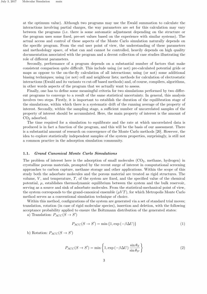
at the optimum value). Although two programs may use the Ewald summation to calculate theinteractions involving partial charges, the way parameters are set for this calculation may varybetween the programs (i.e. there is some automatic adjustment depending on the structure orthe program uses some fixed, pre-set values based on the experience with similar systems). Theactual access and control of these aspects of the Monte Carlo simulation naturally depends onthe specific program. From the end user point of view, the understanding of these parametersand methodology space, of what can and cannot be controlled, heavily depends on high qualitydocumentation associated with the program and a decent collection of case studies illustrating therole of different parameters.

Secondly, performance of a program depends on a substantial number of factors that makeconsistent comparison quite difficult. This include using (or not) pre-calculated potential grids ormaps as oppose to the on-the-fly calculation of all interactions; using (or not) some additionalbiasing techniques; using (or not) cell and neighbour lists; methods for calculation of electrostaticinteractions (Ewald and its variants vs cut-off based methods) and, of course, compilers, algorithms,in other words aspects of the program that we actually want to assess.

Finally, one has to define some meaningful criteria for two simulations performed by two differ-ent programs to converge to a result of the same statistical uncertainty. In general, this analysisinvolves two steps. Firstly, it is important to establish the duration of the equilibration stage ofthe simulations, within which there is a systematic drift of the running average of the property ofinterest. Secondly, within the sampling stage, a sufficient number of uncorrelated samples of theproperty of interest should be accumulated. Here, the main property of interest is the amount ofCO2 adsorbed.

The time required for a simulation to equilibrate and the rate at which uncorrelated data isproduced is in fact a function of the program, and this will be the basis of our assessment. Thereis a substantial amount of research on convergence of the Monte Carlo methods [20]. However, theidea to explore statistically independent samples of the system properties, surprisingly, is still nota common practice in the adsorption simulation community.

1.1. Grand Canonical Monte Carlo Simulations

The problem of interest here is the adsorption of small molecules (CO2, methane, hydrogen) incrystalline porous materials, prompted by the recent surge of interest in computational screeningapproaches to carbon capture, methane storage and other applications. Within the scope of thisstudy both the adsorbate molecules and the porous material are treated as rigid structures. Thevolume, V , and temperature, T , of the system are fixed, and the specified value of the chemicalpotential, µ, establishes thermodynamic equilibrium between the system and the bulk reservoir,serving as a source and sink of adsorbate molecules. From the statistical-mechanical point of view,the system corresponds to the grand-canonical ensemble (µV T ), for which Metropolis Monte Carlomethod serves as a conventional simulation technique of choice.

Within this method, configurations of the system are generated via a set of standard trial moves;translation, rotation (in case of rigid molecular species), insertion and deletion, with the followingacceptance probability applied to ensure the Boltzmann distribution of the generated states:

a) Translation: PACC(S → S′)

PACC(S → S′) = min {1, exp (−β∆U)} (1)

b) Rotation: PACC(S → S′)

PACC(S → S′) = min

{1, exp (−β∆U)

sin θSsin θS′

}(2)

3

July 3, 2017 Molecular Simulation main

c) Insertion: PACC(Na → Na + 1)

PACC(Na → Na + 1) = min

{1,

βfV

Na + 1exp (−β∆U)

}(3)

d) Deletion: PACC(Na → Na − 1)

PACC(Na → Na − 1) = min

{1,

Na

βfVexp(−β∆U)

}(4)

where U represents the potential energy, Na, and V are the number of molecules and volumerespectively, β is the reciprocal thermodynamic temperature, 1/kBT , with kB being the Boltzmannconstant; θ is an Euler angle of the rigid body rotation as defined in Ref [21], f is the fugacity ofthe adsorbing species, which is related to the chemical potential as:

f =qrotβΛ3

exp (βµ) (5)

where qrot is the rotational partition function for a single rigid molecule, equal to 1 for a singleparticle molecule, and Λ is the thermal de Broglie wavelength:

Λ =

(βh2

2πm

) 1

2

(6)

where h is Planck’s constant and m is the molecule mass [21].

2. Methodology

2.1. Case study: CO2 adsorption in IRMOF-1

As has been already discussed in the introduction, computational screening and optimisation ofMOFs and ZIFs for carbon capture applications has been a rapidly developing area of research,driven by both the new opportunities emerging in the material science and the societal importanceof the problem. For this reason, the adsorption of CO2 in IRMOF-1 was selected as the case study.IRMOF-1 is one of the earliest reported MOFs, with a substantial amount of experimental andsimulation data accumulated on its structural and adsorptive properties [22–24].

The study of Walton et al. [24] provides one of the first examples of both experimental andsimulation studies of CO2 adsorption in a MOF (specifically, IRMOF-1). Six adsorption isothermswere reported at 195K, 208K, 218K, 233K, 273K and 298K. Two isotherms at lower temperatures(195K and 208K) feature a sharp transition of the adsorbed density associated with the capillarycondensation of CO2 within the pores of IRMOF-1. The authors argued that it was the Coulombicterm of the fluid-fluid interactions responsible for the shape of the isotherms.

Following this original study, CO2 adsorption in IRMOF-1 at 208K has been used as a tuto-rial case study in Sarkisov’s group for incoming research students and staff. The location of thetransition, as well as the other features of the isotherm, proved to be sensitive to the parametersof the model, cut-off distances, and interaction terms included. For example, in the original studyby Walton et al. [24] the Coulombic interactions between CO2 and IRMOF-1 were not consid-ered, and yet, if included, they shift the isotherm toward lower pressure values. In fact, one ofthe motivations for this study was the significant amount of effort and attention to detail required

4

July 3, 2017 Molecular Simulation main

Table 1.: Summary of the GCMC programs studied.

Program Version License Citation Energy Grid Parallel capability

Cassandra 1.2 GPL v3 Shah and Maginn [26] × OpenMPDL Monte 2.0.1 Custom Purton et al. [27] × MPIMusic 4.0 GPL v2 Gupta et al. [28] X ×Raspa 2.0 GPL v3 Dubbeldam et al. [29] X ×Towhee 7.1.0 GPL v2 Martin [30] × MPI

for different programs to generate exactly the same result. This highlighted the importance of theconsistency between the parameters and methods used, and prompted us to produce and documentthis comparison for other available programs. Hence, in the case study we will focus specifically onCO2 adsorption at 208K.

2.2. Programs under consideration

The special issue of the Molecular Simulation [16], in particular the review by Dubbeldam et al. [25]and our own experience helped us to identify five commonly used, free programs for molecularsimulation of adsorption. All programs are distributed under a GNU GPL license, except DL Montewhich is distributed under a custom academic license which enables it to be used freely for academicand other non-commercial work. The license for DL Monte does not allow distribution of the sourcecode to third parties. This may lead to obstacles in the future in reproducing scientific data whichrequires consistency in both the simulation setups as well as in the program used to execute thesesetups.

The programs studied and their relevent capabilities are summarised in Table 1, while for thecomplete description of all capabilities within each program we refer the reader to the respectiveoriginal publications. It should be emphasised that at no point have we made any alterations tothe source code of the programs under study. We have downloaded each program as it is madeavailable to users and treated it strictly as a black box.

All simulations were ran on identical hardware, using single cores of Intel Xeon E5 2360 v3 nodes,running Scientific Linux version 7.2. Each program was compiled using version 16.0 of the Intelcompilers with the compilation flags ‘-O3 -xcore-AVX2 -ip -ipo’. This combination of softwareand hardware is typical of most modern high performance CPU based supercomputers.

2.2.1. Energy grids and energy-bias GCMC

The calculation of pairwise energies between atoms is by far the single most time consuming stepin the process of GCMC simulation. For a single fluid atom i the contribution to potential energycan be expressed as:

U(ri) =∑

j∈fluidU(rij) +

∑j∈solid

U(rij) (7)

where U represents the potential energy, r the position of an atom, i and j are indices of theatoms, and the two summations are performed over fluid atoms and solid atoms respectively.Since the porous material considered in this study is treated as a rigid structure, it is possible toprecalculate and store solid–fluid interactions. As described elsewhere [31], the simulation volumecan be divided into a regular grid and for each atom type in the adsorbate the correspondingpotential grid is calculated by placing the probe atom onto each grid point and calculating itsinteraction with the solid framework. In case of Coulombic interactions the probe placed in the grid

5

July 3, 2017 Molecular Simulation main

is a single +1 charge. Although it requires a set of additional ‘upfront’ calculations, this procedureis needed only once for all pressure points and temperatures. The potential energy contribution ofa single fluid atom can then be given as:

U(ri) ≈∑

j∈fluidU(rij) + Ugrid(ri) (8)

where the summation is now only performed over other fluid atoms, while the solid–fluid interac-tion is approximated by interpolating within the potential grid, alleviating the need for on-the-flycalculations of the solid–fluid interactions. We will refer to this element of the simulation setup asan energy grid, however it is also known as a potential map [28]. Of the programs examined in thiswork, only Raspa and Music are capable of using this technique.

Using energy grids also opens a possibility for the improvement of sampling efficiency via so-called energy-biasing techniques [32]. Here it is recognised that the solid structure of the framework(zeolite or MOF) may occupy a substantial portion of the simulation cell and choosing a positionfor the potential molecule insertion at random will likely lead to a large number of rejections (due tothe positions overlapping with the structure of the material). Furthermore, certain positions withinthe available porous space will be preferred for the insertion (at an optimal distance from the atomsof the framework), compared to other locations, such as in the center of a large cavity where theinteractions with the framework structure can be quite weak. Hence the idea of the energy-biasingmethod: bias selection of the trial locations for the molecule insertion towards regions of favourableinteraction with the framework structure. For this the location of the insertion is selected from wcubelets according to a weight assigned to each cubelet. Specifically, this weight is based on theenergy of interaction Ugrid(rz) of the probe atom placed in the center of cubelet z within theframework:

ηz =exp (−βUgrid (rz))∑

y=1,w exp (−βUgrid (ry))(9)

where the sum in the denominator is over all grids. This method requires a single energy gridfor a probe atom of choice and naturally, if the program uses energy grids in general, it should alsoinvoke energy biasing as described above since it does not require any additional calculation. Inparticular, this approach is used by Music [28].

2.2.2. Parallelism

Two of the programs investigated have the ability to accelerate simulations through using multipleCPU cores. Cassandra uses OpenMP to distribute the calculation of contributions to the totalenergy, both Lennard-Jones and electrostatics. For the Lennard-Jones contribution within thesummation of Equation 7, it is possible to assign cores to different j indices and calculate eachcontribution simultaneously. For electrostatics an Ewald summation is used, and it is possible tocalculate different k-vectors independently across different cores. OpenMP is a shared memoryprotocol, which limits the extent to which the problem can be split to the number of cores ona single node, typically around 12–24. DL Monte uses a similar strategy, however it parallelisescalculation of the electrostatic interactions only and uses MPI, rather than OpenMP. Towhee alsouses MPI, but instead of parallel execution of a single simulation, it runs several parallel simulationsfor each point on the adsorption isotherm in a so-called jobfarm or task-based parallelism fashion.MPI is a distributed memory paradigm, and so there is no upper limit on the number of cores whichcan be included, although there will be inevitably diminishing returns in terms of computational

6

July 3, 2017 Molecular Simulation main

efficiency.

2.3. Forcefield and simulation setup details

For the selected system of CO2 in IRMOF-1 at 208K we consider three different forcefield setups.In the first setup only Lennard-Jones interactions between CO2 molecules and between CO2 andIRMOF-1 are considered. In the second setup, we further include Coulombic interactions betweenthe molecules of CO2. The final setup has all interaction terms considered, including the CoulombicCO2–IRMOF-1 contribution. This three-level approach allows us to revisit the issue of the role ofthe different terms in the adsorption behavior of CO2 in IRMOF-1 and individually benchmarkthe computational cost associated with the different terms of the interaction energy.

Pressures of 5, 10, 20, 30, 40, 50, 60, and 70 kPa are modelled, with the Peng-Robinson equationof state [33] used to calculate the fugacity and chemical potential of the fluid phase across allprograms. The solid framework consists of 2×2×2 replicas of the crystal unit cell for IRMOF-1,resulting in 3392 atoms of the framework, and up to 1600 CO2 molecules at the highest loadings.Here we use DREIDING [34] parameters for the atoms of IRMOF-1, charges for IRMOF-1 fromYazaydın et al. [35] and TraPPE [36] parameters for CO2.

While the exact implementation of the MC moves is beyond our control, we have attemptedto make the simulation setups as consistent as possible across all programs. All analysis in thiswork is based on the number of MC steps. Raspa instead defines simulation length as a numberof cycles, where a cycle is min(20, N) attempted MC moves, where N is the number of moleculesin the system. Throughout this work we have translated cycles to steps through knowing thenumber of adsorbed molecules. Each MC step has an equal probability of performing an insertion,deletion, rotation or translation move. All the parameters and the details of the simulation setupsare provided as case studies in the Supplementary Material.

3. Defining computational performance

For any meaningful comparison of the performance of different simulation programs, we first needto precisely define how it is measured. In benchmarks of molecular dynamics (MD) simulations itis typical to express performance as a measure of the number of time steps that a program cancomplete in a given time [37]. Two different programs using the time step of the same size andsimulate the same number of time steps should in principle explore the same volume of the phasespace and arrive at the same statistical averages of the properties of interest. From this point ofview, the number of MD steps peformed per unit time can be seen as a direct measurement of datagenerated per unit time.

The situation is different in Monte Carlo simulations, where each step represents an attemptedchange in the system which may or may not be accepted. Equations 1 to 4 provide the foundationfor the most basic Metropolis algorithm, however different programs may have more advancedacceptance criteria which aim to increase the sampling efficiency through various type of biasing.Although, more complex biasing moves may come with an additional computational cost, theresulting simulation scheme may be much more efficient in sampling the phase space.

Therefore depending on the exact implementation of MC moves within a program a fixed numberof steps may traverse a differing volume of the phase space. This means that a direct comparison ofthe rate with which an MC program performs a fixed number of steps, similarly to MD simulations,is an incomplete metric of performance. Instead, we must measure both the rate with which stepsare performed as well as the rate with which these steps traverse the phase space to arrive to theexpected statistical averages. As we will further argue later in this section, it is a product of thesetwo rates which quantifies the performance of the program.

Each GCMC simulation consists of two stages. In the first, so-called equilibration stage, the

7

July 3, 2017 Molecular Simulation main

0 0.5 1.0 1.5 2.0 2.5

Number of MC steps (×108)

100

120

140

Na(m

ol/uc)

Mean and variancefrom final half

Figure 1.: Illustration of the procedure for the location of the equilibration stage in an MC sim-ulation. Data taken from a simulation at 70 kPa, forcefield setup 1, performed using Music. Theblue line represents the rolling mean of the number of adsorbed molecules (over 20,000 steps) asa function of the number of MC steps. Instantaneous values of the number of adsorbed moleculesare not shown for clarity. The vertical dotted line indicates the final half of the data set, the hor-izontal black dashed line represents the value of the mean from this region while the red dashedline underneath corresponds to two standard deviations below the mean. The red dot delineatesthe equilibration and sampling stages, according to the procedure described in the text.

properties of the system drift from the initial conditions until they stabilise around some averagevalues. Once the system reached this point, we can commence the second, sampling stage, wherestatistical averages of the properties of interest are accumuluated. To assess computational pefor-mance of the program we need to measure how long it takes for the program to reach the samplingstage and then apply our definition of the performance of a Monte Carlo simulation in terms ofdata generated per MC step in the second stage of the simulation.

In the following three sections we will describe our methodology for measuring computationalperformance, from defining the equilibration and sampling stages of a simulation, defining the rateat which sampling occurs and the method by which we timed these processes. We have endeavouredto make this analysis as automated as possible, both to make the results as impartial as possible andto ensure that this analysis can be reproduced independently by other researchers. All preparationof inputs and implementation of the analysis was achieved using a combination of the Pythonpackages datreant [38], matplotlib [39], MDAnalysis [40, 41], numpy [42] and pandas [43]. Examplesof the analysis performed are also made available in the Supplementary Material.

3.1. Equilibration stage

In this section we explain how we determine the duration of the equilibration stage in a GCMCsimulation. Figure 1 shows a typical evolution of the number of adsorbed molecules in the systemas a function of the number of MC steps. Initially the system is empty, and as the simulationprogresses the number of molecules rapidly increases to about 135 molecules. For the remainingpart of the run, the instantaneous values of the number of molecules in the system fluctuate aroundsome average value. The visual inspection of Figure 1 gives us a fairly good understanding of theboundary between the equilibration and sampling stages. In fact, in the MC community such avisual inspection is still commonly used to identify the number of steps required for equilibration.However, we are interested in having an automated procedure to identify this boundary.

This procedure works as follows. We first run a very long simulation, typically around 250×106

MC steps. The results of the second half of the long simulation are used to estimate the mean andstandard deviation of the number of molecules at this pressure. At this stage it is important to

8

July 3, 2017 Molecular Simulation main

emphasise that calculating the standard deviation in this fashion significantly underestimates thetrue value, as there will be correlation between data points, as we will discuss later in the article.However, for the purposes of the algorithm that simply intends to locate the equilibration stagethis crude approach suffices. As an additional test to ensure that the sampling stage is reached, astraight line of best fit is constucted through the data in the second half of the simulation and thedifference between the starting point of this line and final point of this line must be less than 5%of the mean value.

We then consider a rolling mean average of the number of molecules in the system using awindow width of 20,000 MC steps. Again, this number may seem rather arbitrary and the statisticalquality of this mean for different programs will be different, but extensive testing of the approachon a number of systems shows that it works well in practice. We then move this rolling averagebackwards from the halfway point until it falls below two standard deviations from the estimatedmean (Figure 1). According to our protocol, this point delineates equilibrium and sampling stages.All MC steps before this point belong to the equilibration stage, while all subsequent points areconsidered to be within the sampling stage.

This process gives us, for each simulation condition in each program, a measure of the numberof MC steps required to reach the sampling stage. We acknowlege that the criteria for defining thetwo stages are fairly arbitrary and alternative algorithms could have been used [44]. However itprovided consistent and sensible results across the data we examined. Moreover it could be usedin a fully automised fashion, removing any human interaction in interpreting the results.

3.2. Sampling stage

As has been discussed, comparison of the computational performance of GCMC programs cannotbe based on a fixed number of MC steps, since it will produce averages of different statistical qualityand uncertainty. Instead we base this analysis on the number of steps required for a program togenerate a certain number of independent, uncorrelated configurations.

For this we consider the normalised autocorrelation function (ACF) of the number of moleculesadsorbed, C(n), shown in Equation 10.

C(n) =〈Na(n0)Na(n0 + n)〉 − 〈Na〉2

〈N2a 〉 − 〈Na〉2

(10)

where angular brackets denote an average over the ensemble, n is the number of the MC stepsand n0 denotes the starting step.

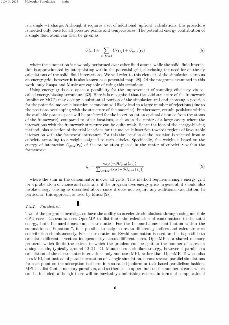
The ACF can then be fitted using a least squares regression to an exponential decay with aconstant τ , Equation 11. As the ACF is inherently noisy for low values of C(n), we identify thefirst point at which it falls below a value of 0.1 and only the initial portion of the function is usedfor fitting. An example of this procedure is illustrated in Figure 2.

C(n) ≈ exp(−nτ

)(11)

This then allows us to define the so-called statistical inefficiency, g [45, 46]:

g = 1 + 2τ (12)

The value g is a measure of the number of MC steps required to move to a statistically novelpoint in the simulation, with any measurement inbetween being correlated and therefore yielding

9

July 3, 2017 Molecular Simulation main

0 1 2 3 4

n (×106)

0.0

0.5

1.0

C(n)

Figure 2.: Illustration of the fitting of the ACF to an exponential decay, using the same datashown in Figure 1. The blue section indicates the portion used for the fitting, while the red sectionindicates the discarded portion of the function. The truncation point is shown as black dashedlines. Black dotted line indicates the function estimated by the fitting procedure.

0 2.5 5.0 7.5 10

m (×106)

0.06

0.12

0.18

0.24

BSE(m

)

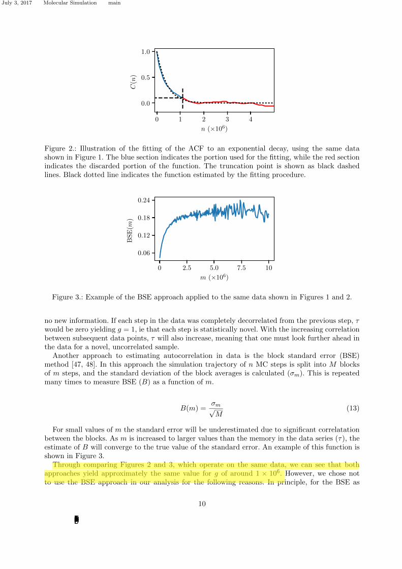
Figure 3.: Example of the BSE approach applied to the same data shown in Figures 1 and 2.

no new information. If each step in the data was completely decorrelated from the previous step, τwould be zero yielding g = 1, ie that each step is statistically novel. With the increasing correlationbetween subsequent data points, τ will also increase, meaning that one must look further ahead inthe data for a novel, uncorrelated sample.

Another approach to estimating autocorrelation in data is the block standard error (BSE)method [47, 48]. In this approach the simulation trajectory of n MC steps is split into M blocksof m steps, and the standard deviation of the block averages is calculated (σm). This is repeatedmany times to measure BSE (B) as a function of m.

B(m) =σm√M

(13)

For small values of m the standard error will be underestimated due to significant correlatationbetween the blocks. As m is increased to larger values than the memory in the data series (τ), theestimate of B will converge to the true value of the standard error. An example of this function isshown in Figure 3.

Through comparing Figures 2 and 3, which operate on the same data, we can see that bothapproaches yield approximately the same value for g of around 1 × 106. However, we chose notto use the BSE approach in our analysis for the following reasons. In principle, for the BSE as

10

July 3, 2017 Molecular Simulation main

a function of m, gradual increase in B is to be followed by a plateau region. At higher valuesof m a significant scattering in B is observed due to the small number of blocks available. Thismakes it difficult, especially in a fully automated procedure, to accurately locate the start of theplateau region. We also observe that in the systems under consideration much longer simulations arerequired to arrive at the same estimate of τ compared to the direct calculation of the ACF. Finally,one of the original arguments advocating the use of BSE was the high computational cost associatedwith directly calculating the ACF [47]. However, through the Wiener–Khinchin theorem [49] it ispossible to calculate this function in a much faster way using the Fourier transformations and ona modern desktop workstation it is now possible to do this in a negligible amount of time. Overall,we find the approach based on the ACF analysis easy to implement in a fully atomatic fashion,and this convenience provides the final decisive arguement in its favour.

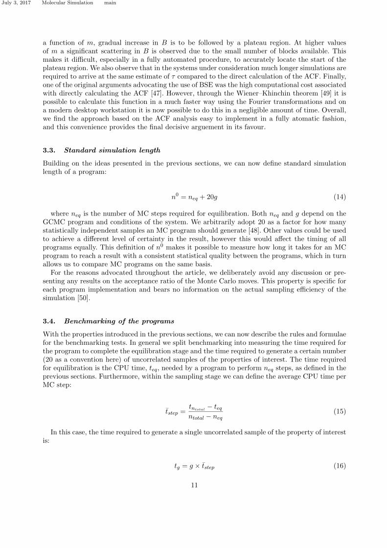
3.3. Standard simulation length

Building on the ideas presented in the previous sections, we can now define standard simulationlength of a program:

n0 = neq + 20g (14)

where neq is the number of MC steps required for equilibration. Both neq and g depend on theGCMC program and conditions of the system. We arbitrarily adopt 20 as a factor for how manystatistically independent samples an MC program should generate [48]. Other values could be usedto achieve a different level of certainty in the result, however this would affect the timing of allprograms equally. This definition of n0 makes it possible to measure how long it takes for an MCprogram to reach a result with a consistent statistical quality between the programs, which in turnallows us to compare MC programs on the same basis.

For the reasons advocated throughout the article, we deliberately avoid any discussion or pre-senting any results on the acceptance ratio of the Monte Carlo moves. This property is specific foreach program implementation and bears no information on the actual sampling efficiency of thesimulation [50].

3.4. Benchmarking of the programs

With the properties introduced in the previous sections, we can now describe the rules and formulaefor the benchmarking tests. In general we split benchmarking into measuring the time required forthe program to complete the equilibration stage and the time required to generate a certain number(20 as a convention here) of uncorrelated samples of the properties of interest. The time requiredfor equilibration is the CPU time, teq, needed by a program to perform neq steps, as defined in theprevious sections. Furthermore, within the sampling stage we can define the average CPU time perMC step:

tstep =tntotal

− teqntotal − neq

(15)

In this case, the time required to generate a single uncorrelated sample of the property of interestis:

tg = g × tstep (16)

11

July 3, 2017 Molecular Simulation main

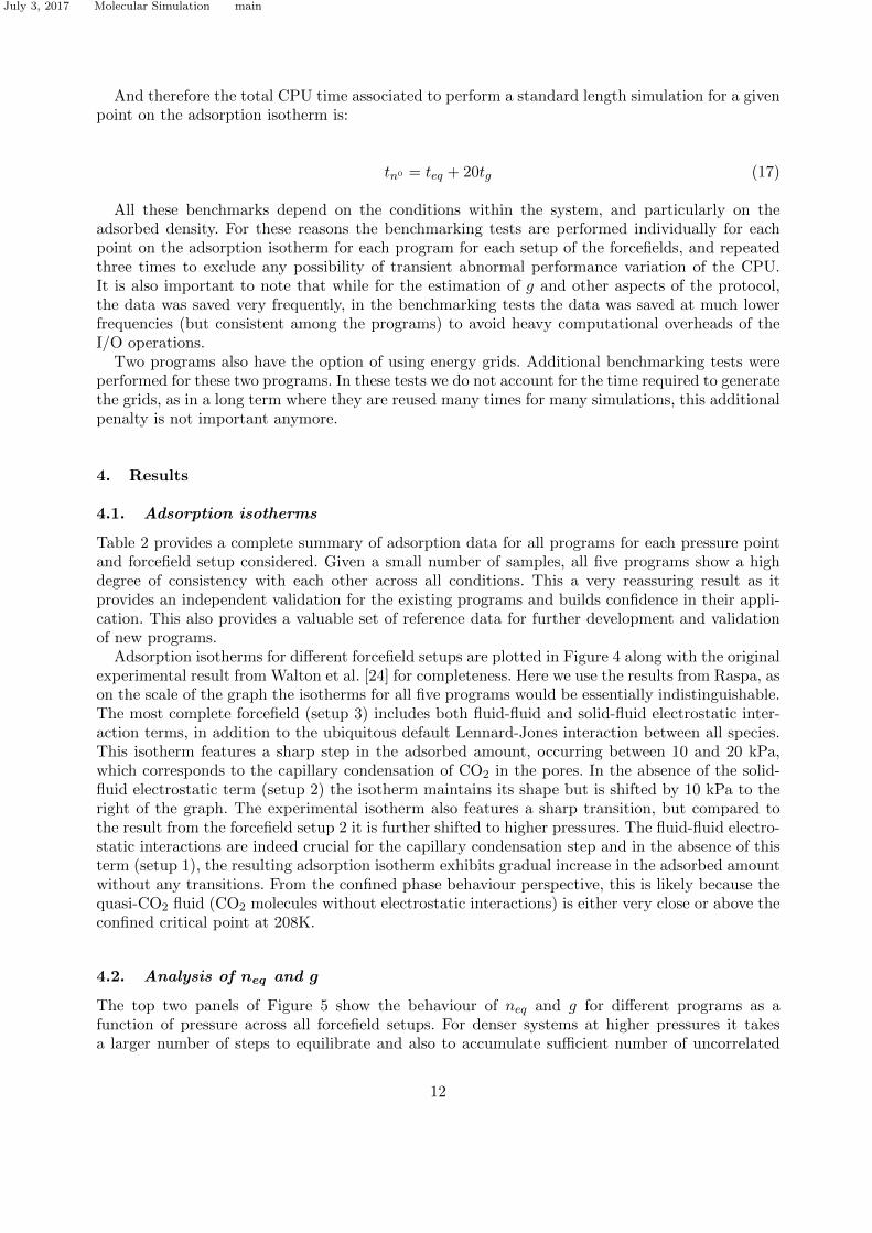
And therefore the total CPU time associated to perform a standard length simulation for a givenpoint on the adsorption isotherm is:

tn0 = teq + 20tg (17)

All these benchmarks depend on the conditions within the system, and particularly on theadsorbed density. For these reasons the benchmarking tests are performed individually for eachpoint on the adsorption isotherm for each program for each setup of the forcefields, and repeatedthree times to exclude any possibility of transient abnormal performance variation of the CPU.It is also important to note that while for the estimation of g and other aspects of the protocol,the data was saved very frequently, in the benchmarking tests the data was saved at much lowerfrequencies (but consistent among the programs) to avoid heavy computational overheads of theI/O operations.

Two programs also have the option of using energy grids. Additional benchmarking tests wereperformed for these two programs. In these tests we do not account for the time required to generatethe grids, as in a long term where they are reused many times for many simulations, this additionalpenalty is not important anymore.

4. Results

4.1. Adsorption isotherms

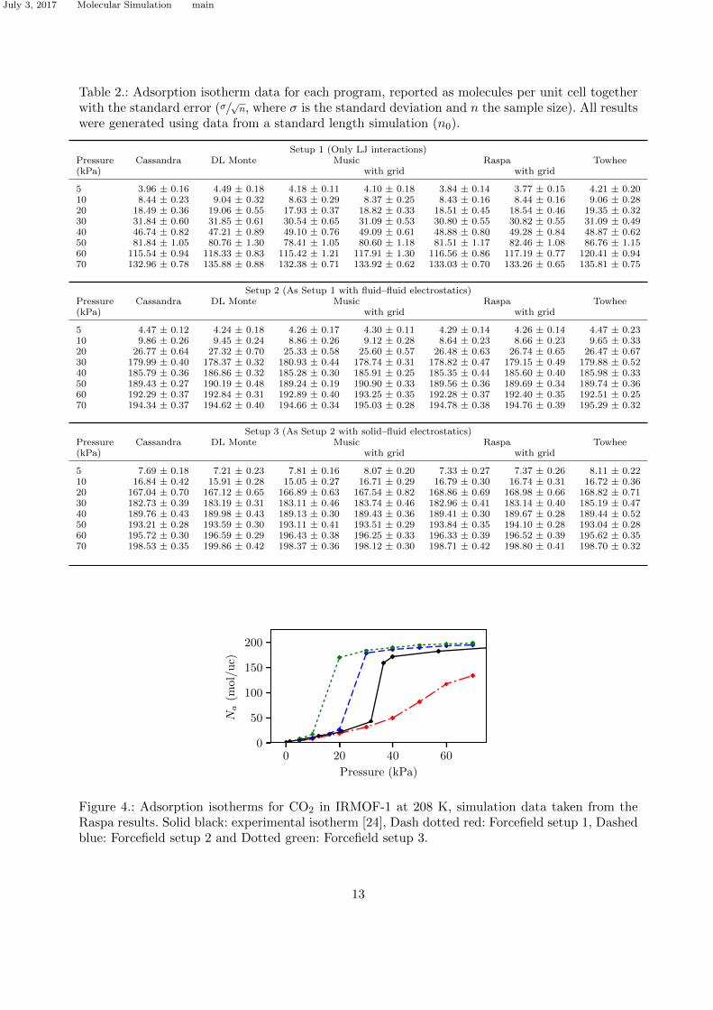
Table 2 provides a complete summary of adsorption data for all programs for each pressure pointand forcefield setup considered. Given a small number of samples, all five programs show a highdegree of consistency with each other across all conditions. This a very reassuring result as itprovides an independent validation for the existing programs and builds confidence in their appli-cation. This also provides a valuable set of reference data for further development and validationof new programs.

Adsorption isotherms for different forcefield setups are plotted in Figure 4 along with the originalexperimental result from Walton et al. [24] for completeness. Here we use the results from Raspa, ason the scale of the graph the isotherms for all five programs would be essentially indistinguishable.The most complete forcefield (setup 3) includes both fluid-fluid and solid-fluid electrostatic inter-action terms, in addition to the ubiquitous default Lennard-Jones interaction between all species.This isotherm features a sharp step in the adsorbed amount, occurring between 10 and 20 kPa,which corresponds to the capillary condensation of CO2 in the pores. In the absence of the solid-fluid electrostatic term (setup 2) the isotherm maintains its shape but is shifted by 10 kPa to theright of the graph. The experimental isotherm also features a sharp transition, but compared tothe result from the forcefield setup 2 it is further shifted to higher pressures. The fluid-fluid electro-static interactions are indeed crucial for the capillary condensation step and in the absence of thisterm (setup 1), the resulting adsorption isotherm exhibits gradual increase in the adsorbed amountwithout any transitions. From the confined phase behaviour perspective, this is likely because thequasi-CO2 fluid (CO2 molecules without electrostatic interactions) is either very close or above theconfined critical point at 208K.

4.2. Analysis of neq and g

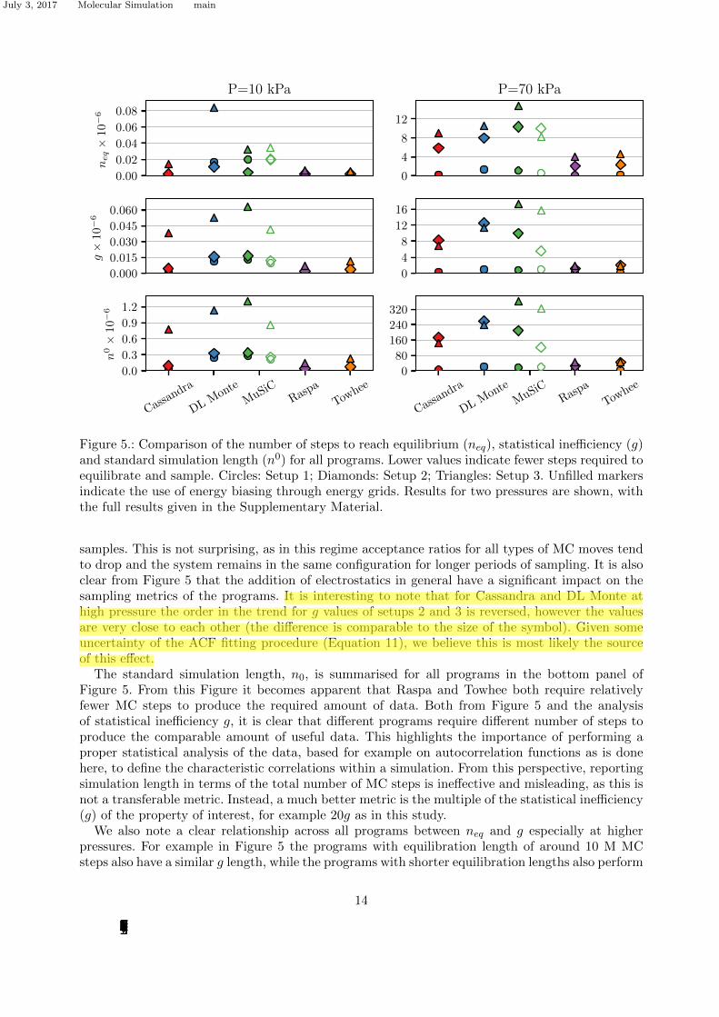
The top two panels of Figure 5 show the behaviour of neq and g for different programs as afunction of pressure across all forcefield setups. For denser systems at higher pressures it takesa larger number of steps to equilibrate and also to accumulate sufficient number of uncorrelated

12

July 3, 2017 Molecular Simulation main

Table 2.: Adsorption isotherm data for each program, reported as molecules per unit cell togetherwith the standard error (σ/

√n, where σ is the standard deviation and n the sample size). All results

were generated using data from a standard length simulation (n0).

Setup 1 (Only LJ interactions)Pressure Cassandra DL Monte Music Raspa Towhee(kPa) with grid with grid

5 3.96 ± 0.16 4.49 ± 0.18 4.18 ± 0.11 4.10 ± 0.18 3.84 ± 0.14 3.77 ± 0.15 4.21 ± 0.2010 8.44 ± 0.23 9.04 ± 0.32 8.63 ± 0.29 8.37 ± 0.25 8.43 ± 0.16 8.44 ± 0.16 9.06 ± 0.2820 18.49 ± 0.36 19.06 ± 0.55 17.93 ± 0.37 18.82 ± 0.33 18.51 ± 0.45 18.54 ± 0.46 19.35 ± 0.3230 31.84 ± 0.60 31.85 ± 0.61 30.54 ± 0.65 31.09 ± 0.53 30.80 ± 0.55 30.82 ± 0.55 31.09 ± 0.4940 46.74 ± 0.82 47.21 ± 0.89 49.10 ± 0.76 49.09 ± 0.61 48.88 ± 0.80 49.28 ± 0.84 48.87 ± 0.6250 81.84 ± 1.05 80.76 ± 1.30 78.41 ± 1.05 80.60 ± 1.18 81.51 ± 1.17 82.46 ± 1.08 86.76 ± 1.1560 115.54 ± 0.94 118.33 ± 0.83 115.42 ± 1.21 117.91 ± 1.30 116.56 ± 0.86 117.19 ± 0.77 120.41 ± 0.9470 132.96 ± 0.78 135.88 ± 0.88 132.38 ± 0.71 133.92 ± 0.62 133.03 ± 0.70 133.26 ± 0.65 135.81 ± 0.75

Setup 2 (As Setup 1 with fluid–fluid electrostatics)Pressure Cassandra DL Monte Music Raspa Towhee(kPa) with grid with grid

5 4.47 ± 0.12 4.24 ± 0.18 4.26 ± 0.17 4.30 ± 0.11 4.29 ± 0.14 4.26 ± 0.14 4.47 ± 0.2310 9.86 ± 0.26 9.45 ± 0.24 8.86 ± 0.26 9.12 ± 0.28 8.64 ± 0.23 8.66 ± 0.23 9.65 ± 0.3320 26.77 ± 0.64 27.32 ± 0.70 25.33 ± 0.58 25.60 ± 0.57 26.48 ± 0.63 26.74 ± 0.65 26.47 ± 0.6730 179.99 ± 0.40 178.37 ± 0.32 180.93 ± 0.44 178.74 ± 0.31 178.82 ± 0.47 179.15 ± 0.49 179.88 ± 0.5240 185.79 ± 0.36 186.86 ± 0.32 185.28 ± 0.30 185.91 ± 0.25 185.35 ± 0.44 185.60 ± 0.40 185.98 ± 0.3350 189.43 ± 0.27 190.19 ± 0.48 189.24 ± 0.19 190.90 ± 0.33 189.56 ± 0.36 189.69 ± 0.34 189.74 ± 0.3660 192.29 ± 0.37 192.84 ± 0.31 192.89 ± 0.40 193.25 ± 0.35 192.28 ± 0.37 192.40 ± 0.35 192.51 ± 0.2570 194.34 ± 0.37 194.62 ± 0.40 194.66 ± 0.34 195.03 ± 0.28 194.78 ± 0.38 194.76 ± 0.39 195.29 ± 0.32

Setup 3 (As Setup 2 with solid–fluid electrostatics)Pressure Cassandra DL Monte Music Raspa Towhee(kPa) with grid with grid

5 7.69 ± 0.18 7.21 ± 0.23 7.81 ± 0.16 8.07 ± 0.20 7.33 ± 0.27 7.37 ± 0.26 8.11 ± 0.2210 16.84 ± 0.42 15.91 ± 0.28 15.05 ± 0.27 16.71 ± 0.29 16.79 ± 0.30 16.74 ± 0.31 16.72 ± 0.3620 167.04 ± 0.70 167.12 ± 0.65 166.89 ± 0.63 167.54 ± 0.82 168.86 ± 0.69 168.98 ± 0.66 168.82 ± 0.7130 182.73 ± 0.39 183.19 ± 0.31 183.11 ± 0.46 183.74 ± 0.46 182.96 ± 0.41 183.14 ± 0.40 185.19 ± 0.4740 189.76 ± 0.43 189.98 ± 0.43 189.13 ± 0.30 189.43 ± 0.36 189.41 ± 0.30 189.67 ± 0.28 189.44 ± 0.5250 193.21 ± 0.28 193.59 ± 0.30 193.11 ± 0.41 193.51 ± 0.29 193.84 ± 0.35 194.10 ± 0.28 193.04 ± 0.2860 195.72 ± 0.30 196.59 ± 0.29 196.43 ± 0.38 196.25 ± 0.33 196.33 ± 0.39 196.52 ± 0.39 195.62 ± 0.3570 198.53 ± 0.35 199.86 ± 0.42 198.37 ± 0.36 198.12 ± 0.30 198.71 ± 0.42 198.80 ± 0.41 198.70 ± 0.32

0 20 40 60

Pressure (kPa)

0

50

100

150

200

Na(m

ol/uc)

Figure 4.: Adsorption isotherms for CO2 in IRMOF-1 at 208 K, simulation data taken from theRaspa results. Solid black: experimental isotherm [24], Dash dotted red: Forcefield setup 1, Dashedblue: Forcefield setup 2 and Dotted green: Forcefield setup 3.

13

July 3, 2017 Molecular Simulation main

0.00

0.02

0.04

0.06

0.08neq×10−6

P=10 kPa

0

4

8

12

P=70 kPa

0.000

0.015

0.030

0.045

0.060

g×10−6

0

4

8

12

16

Cassa

ndra

DLMon

te

MuSiC

Raspa

Towh

ee0.0

0.3

0.6

0.9

1.2

n0×10−6

Cassa

ndra

DLMon

te

MuSiC

Raspa

Towh

ee0

80

160

240

320

Figure 5.: Comparison of the number of steps to reach equilibrium (neq), statistical inefficiency (g)and standard simulation length (n0) for all programs. Lower values indicate fewer steps required toequilibrate and sample. Circles: Setup 1; Diamonds: Setup 2; Triangles: Setup 3. Unfilled markersindicate the use of energy biasing through energy grids. Results for two pressures are shown, withthe full results given in the Supplementary Material.

samples. This is not surprising, as in this regime acceptance ratios for all types of MC moves tendto drop and the system remains in the same configuration for longer periods of sampling. It is alsoclear from Figure 5 that the addition of electrostatics in general have a significant impact on thesampling metrics of the programs. It is interesting to note that for Cassandra and DL Monte athigh pressure the order in the trend for g values of setups 2 and 3 is reversed, however the valuesare very close to each other (the difference is comparable to the size of the symbol). Given someuncertainty of the ACF fitting procedure (Equation 11), we believe this is most likely the sourceof this effect.

The standard simulation length, n0, is summarised for all programs in the bottom panel ofFigure 5. From this Figure it becomes apparent that Raspa and Towhee both require relativelyfewer MC steps to produce the required amount of data. Both from Figure 5 and the analysisof statistical inefficiency g, it is clear that different programs require different number of steps toproduce the comparable amount of useful data. This highlights the importance of performing aproper statistical analysis of the data, based for example on autocorrelation functions as is donehere, to define the characteristic correlations within a simulation. From this perspective, reportingsimulation length in terms of the total number of MC steps is ineffective and misleading, as this isnot a transferable metric. Instead, a much better metric is the multiple of the statistical inefficiency(g) of the property of interest, for example 20g as in this study.

We also note a clear relationship across all programs between neq and g especially at higherpressures. For example in Figure 5 the programs with equilibration length of around 10 M MCsteps also have a similar g length, while the programs with shorter equilibration lengths also perform

14

July 3, 2017 Molecular Simulation main

0.00

0.01

0.02

0.03

0.04t e

q(hours)

P=10 kPa

08

16243240

P=70 kPa

0.0

0.8

1.6

2.4

3.2

t step×106(hours)

0.01.53.04.56.0

Cassa

ndra

DLMon

te

MuSiC

Raspa

Towh

ee0.00

0.01

0.02

0.03

0.04

t g(hours)

Cassa

ndra

DLMon

te

MuSiC

Raspa

Towh

ee08

16243240

Figure 6.: Top panel: time required to reach equilibrium, teq. Middle panel: time required to perform1 M sampling steps. Bottom panel: time required to produce g sampling steps. Legend as in Figure 5,unfilled markers indicate the use of energy grids. Results for two pressures are shown, with the fullresults given in the Supplementary Material.

a statistical decorrelation faster. This prompts us to speculate that the sampling rate in MC stepsof a program can be roughly assessed from neq alone.

4.3. Program timing

Now that we have defined the required number of MC steps to perform equivalent simulations, wecan proceed to measuring the time this will take to calculate, this is shown in Figure 6. Immediatelyapparent is that simulations at higher loadings take longer to complete. This is not surprising asat higher loadings larger number of intermolecular interactions must be calculated with each MCmove.

The time to produce sampling MC steps is shown in Figure 6 and from this we see again a largedifference between programs to perform a seemingly similar task. This time however the order ofprograms is reversed compared to Figure 5, which clearly indicates that whilst programs such asRaspa and Towhee are able to produce more data with a fixed number of steps, it also takes longer tocalculate such steps. Conversely we can see that the two programs with the longest decorrelationtimes, Music and DL Monte, are also the two fastest programs to complete a fixed number ofsampling steps. Clearly there is a difference between the various programs in the definition of whatconstitutes a single MC step, as without any biasing neq should be identical between programs asit relies on random insertions. This again underlines the importance of the steps to decorrelation(g) as previously measured, by naively benchmarking the time to perform a fixed number of MCsteps we might arrive at the wrong conclusion.

15

July 3, 2017 Molecular Simulation main

Cassa

ndra

DLMon

te

MuSiC

Raspa

Towh

ee0

300

600

900

1200

t n0(hours)

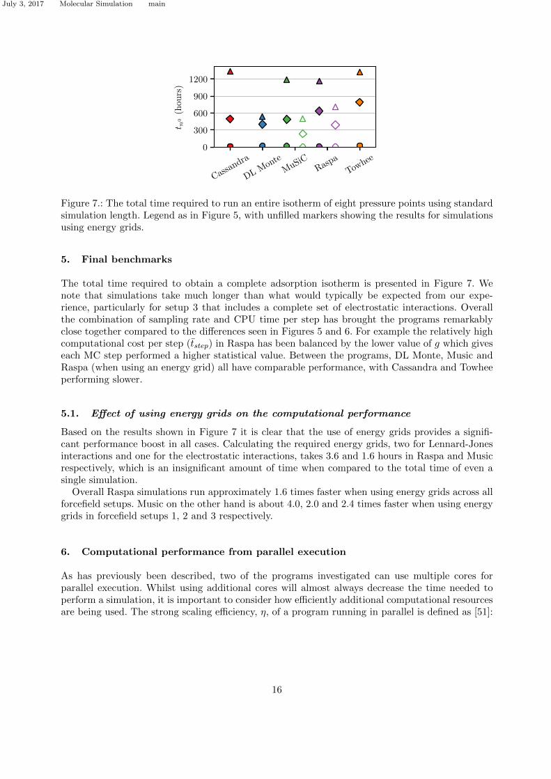
Figure 7.: The total time required to run an entire isotherm of eight pressure points using standardsimulation length. Legend as in Figure 5, with unfilled markers showing the results for simulationsusing energy grids.

5. Final benchmarks

The total time required to obtain a complete adsorption isotherm is presented in Figure 7. Wenote that simulations take much longer than what would typically be expected from our expe-rience, particularly for setup 3 that includes a complete set of electrostatic interactions. Overallthe combination of sampling rate and CPU time per step has brought the programs remarkablyclose together compared to the differences seen in Figures 5 and 6. For example the relatively highcomputational cost per step (tstep) in Raspa has been balanced by the lower value of g which giveseach MC step performed a higher statistical value. Between the programs, DL Monte, Music andRaspa (when using an energy grid) all have comparable performance, with Cassandra and Towheeperforming slower.

5.1. Effect of using energy grids on the computational performance

Based on the results shown in Figure 7 it is clear that the use of energy grids provides a signifi-cant performance boost in all cases. Calculating the required energy grids, two for Lennard-Jonesinteractions and one for the electrostatic interactions, takes 3.6 and 1.6 hours in Raspa and Musicrespectively, which is an insignificant amount of time when compared to the total time of even asingle simulation.

Overall Raspa simulations run approximately 1.6 times faster when using energy grids across allforcefield setups. Music on the other hand is about 4.0, 2.0 and 2.4 times faster when using energygrids in forcefield setups 1, 2 and 3 respectively.

6. Computational performance from parallel execution

As has previously been described, two of the programs investigated can use multiple cores forparallel execution. Whilst using additional cores will almost always decrease the time needed toperform a simulation, it is important to consider how efficiently additional computational resourcesare being used. The strong scaling efficiency, η, of a program running in parallel is defined as [51]:

16

July 3, 2017 Molecular Simulation main

η (c) =ideal run time

actual run time

=trun(1)/c

trun(c)

(18)

where c is the number of cores and trun the runtime of a program as a function of the numberof computer cores used.

As an alternative to running a single simulation in parallel, we can consider running differentportions of the total number of MC steps of a long run using different instances of a program.In the context of adsorption simulation using GCMC methods, we also need to be aware that inthe system which is always initiated from an empty unit cell, a certain portion of a single runwill be spent on the equilibration stage. For example a simulation of 106 equilibration steps and107 sampling steps could be split into two simulations, consisting of 106 equilibration steps and5×106 sampling steps each. As long as the smaller parallel runs and one long run produce the samenumber of uncorrelated samples, these two modes of execution are equivalent and this approachis a common practice in the MD community [52]. In the previous example of splitting a long runinto two runs, this doubles the number of steps and computational effort spent on equilibration.

This is implemented in Towhee, however this can also be done outside of the program by simplysetting up and running multiple simulations as independent tasks. Mathematically, assuming trunis simply proportional to the number of MC steps, the efficiency of these parallel tasks can beestimated as

η(c) =trun(1)/c

trun(c)

≈(neq + nsamp)/c

neq + nsamp/c=

1 + nsamp

neq

c+ nsamp

neq

(19)

where neq refers to the number of equilibration steps, and nsamp the number of sampling steps.The efficiency at a given number of cores can be seen to rely on the ratio of sampling steps toequilibration steps, with relatively longer equilibration periods leading to less efficient usage ofparallel cores. Splitting single simulations into separate tasks has previously been dismissed dueto the long equilibration times [27]. Our previous results however show that typically neq and gare of the same order of magnitude, therefore long equilibration stages simply indicate that longsampling stages are also required. In these circumstances, task based parallelism is a valid route toaccelerate simulations. Based on our previously discussed observations and our defined standardsimulation length (n0), we have used a nsamp/neq ratio of 20 to estimate the efficiency of task basedparallelism.

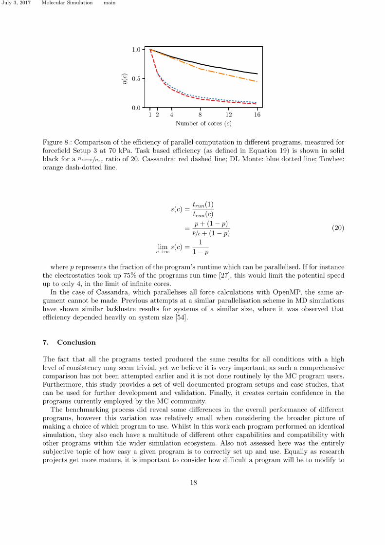
From Figure 8 it can be seen that both Cassandra and DL Monte do not efficiently use parallelcores, and these results are in agreement with the previously published results for DL Monte [27].Under these circumstances, for the simulation of a single pressure point, computational resourceswould be much better used by running many serial tasks and collating the results at the end ofthe simulations. This is shown in the results for Towhee, where the efficiency is much greater thanthe other two programs.

In the case of DL Monte, where only the electrostatic interactions are parallelised, the poorefficiency can be explained by considering Amdahl’s Law [53] which states that the limit of speedup(s) for a program is given as:

17

July 3, 2017 Molecular Simulation main

1 2 4 8 12 16

Number of cores (c)

1.0

0.5

0.0

η(c)

Figure 8.: Comparison of the efficiency of parallel computation in different programs, measured forforcefield Setup 3 at 70 kPa. Task based efficiency (as defined in Equation 19) is shown in solidblack for a nsamp/neq ratio of 20. Cassandra: red dashed line; DL Monte: blue dotted line; Towhee:orange dash-dotted line.

s(c) =trun(1)

trun(c)

=p+ (1− p)p/c + (1− p)

limc→∞

s(c) =1

1− p

(20)

where p represents the fraction of the program’s runtime which can be parallelised. If for instancethe electrostatics took up 75% of the programs run time [27], this would limit the potential speedup to only 4, in the limit of infinite cores.

In the case of Cassandra, which parallelises all force calculations with OpenMP, the same ar-gument cannot be made. Previous attempts at a similar parallelisation scheme in MD simulationshave shown similar lacklustre results for systems of a similar size, where it was observed thatefficiency depended heavily on system size [54].

7. Conclusion

The fact that all the programs tested produced the same results for all conditions with a highlevel of consistency may seem trivial, yet we believe it is very important, as such a comprehensivecomparison has not been attempted earlier and it is not done routinely by the MC program users.Furthermore, this study provides a set of well documented program setups and case studies, thatcan be used for further development and validation. Finally, it creates certain confidence in theprograms currently employed by the MC community.

The benchmarking process did reveal some differences in the overall performance of differentprograms, however this variation was relatively small when considering the broader picture ofmaking a choice of which program to use. Whilst in this work each program performed an identicalsimulation, they also each have a multitude of different other capabilities and compatibility withother programs within the wider simulation ecosystem. Also not assessed here was the entirelysubjective topic of how easy a given program is to correctly set up and use. Equally as researchprojects get more mature, it is important to consider how difficult a program will be to modify to

18

July 3, 2017 Molecular Simulation main

allow it to meet future, more specific needs. When selecting a MC program to use all these variousfactors must also be taken into consideration alongside considering the computational performance.

Whilst it is common to report the lengths of MC simulations as a number of steps, we have shownthat this metric is not transferable between different programs, and therefore between researchgroups who have built an intuition for a given program. Instead, we argue it would be much moreuseful and important for reproducibility of the results to report simulation length as a multiple ofg, along with the value of g for each specific simulation, which reflects the quantity of sampling thathas been performed. When analysing a MC simulation, calculating the length of the simulation interms of g allows us to define if enough data has been gathered and for the level of confidence inthe result to be quantified. We have found that for systems of this type that g can be estimated asapproximately the same order of magnitude as neq, and this can be used to estimate the requiredlength of additional simulation required once a simulation has reached equilibrium.

The varying relative value in data of an MC step simply reflects the fact that there are differentstrategies to implement an MC move. From a program development point of view it would bevery misleading to concentrate on the required walltime for a single move in order to optimisethe performance of a program. Instead, the larger picture of the entire sampling process mustbe considered. The choice of which MC moves to use and the proportion of each move to useremains open for investigation, however using the metrics developed in this work it should now bepossible to accurately quantify the effects these moves make. This will become especially true whenconsidering more complicated MC moves, such as configuration bias moves for flexible molecules.

Our further recommendations can be summarised as follows. Energy grids must definitely beused when possible as they clearly provide a quick and efficient way to substantially increasecomputational performance of the MC programs in the context of adsorption problems. The scopefor increasing performance through parallelism within a program seems limited, due mostly to theinherently small system sizes, and measured performances of existing implementations show poorefficiency. In fact, we argue that in the context of adsorption problems and computational screeningof materials, parallel execution of multiple instances of the process offers much better efficiencyand overall speed up for a fixed amount of computational resources.

7.1. Acknowledgements

The authors would like to thank Dr. David Dubbeldam, Dr. Martin Sweatman, Dr. Daniel Sideriusand Prof. Randy Snurr for useful discussions and advice. The work has made use of resourcesprovided by the Edinburgh Compute and Data Facility (ECDF; www.ecdf.ed.ac.uk)

7.2. Disclosure

No potential conflict of interest was reported by the authors.

7.3. Funding

This work was supported by the EPSRC funding Grant EP/N007859/1

References

[1] Wilmer CE, Leaf M, Lee CY, et al. Large-scale screening of hypothetical metal-organic frameworks.Nature Chemistry. 2012 Feb;4:83–89.

[2] Lin LC, Berger AH, Martin RL, et al. In silico screening of carbon-capture materials. Nature materials.2012;11:633–641.

19

July 3, 2017 Molecular Simulation main

[3] Keskin S, Sholl DS. Efficient methods for screening of metal organic framework membranes for gasseparations using atomically detailed models. Langmuir. 2009;25:11786–11795.

[4] Jiang J, Babarao R, Hu Z. Molecular simulations for energy, environmental and pharmaceutical appli-cations of nanoporous materials: From zeolites, metal–organic frameworks to protein crystals. ChemicalSociety Reviews. 2011;40:3599–3612.

[5] Yang Q, Liu D, Zhong C, et al. Development of computational methodologies for metalorganic frame-works and their application in gas separations. Chemical Reviews. 2013;113:8261–8323.

[6] Jiang J. Molecular simulations in metalorganic frameworks for diverse potential applications. MolecularSimulation. 2014;40:516–536.

[7] Fischer M, Gomes JR, Jorge M. Computational approaches to study adsorption in MOFs with unsat-urated metal sites. Molecular Simulation. 2014;40:537–556.

[8] Erucar I, Manz TA, Keskin S. Effects of electrostatic interactions on gas adsorption and permeabilityof MOF membranes. Molecular Simulation. 2014;40:557–570.

[9] Chen L, Morrison CA, Duren T. Improving predictions of gas adsorption in metalorganic frameworkswith coordinatively unsaturated metal sites: Model potentials, ab initio parameterization, and GCMCsimulations. The Journal of Physical Chemistry C. 2012;116:18899–18909.

[10] Dzubak AL, Lin LC, Kim J, et al. Ab initio carbon capture in open-site metalorganic frameworks.Nature Chemistry. 2012;4:810–816.

[11] Kim J, Lin LC, Lee K, et al. Efficient determination of accurate force fields for porous materials usingab initio total energy calculations. The Journal of Physical Chemistry C. 2014;118:2693–2701.

[12] Haldoupis E, Borycz J, Shi H, et al. Ab initio derived force fields for predicting CO2 adsorption andaccessibility of metal sites in the metalorganic frameworks M-MOF-74 (M = Mn, Co, Ni, Cu). TheJournal of Physical Chemistry C. 2015;119:16058–16071.

[13] Becker TM, Heinen J, Dubbeldam D, et al. Polarizable force fields for CO2 and CH4 adsorption inM-MOF-74. The Journal of Physical Chemistry C. 2017;121:4659–4673.

[14] Banu AM, Friedrich D, Brandani S, et al. A multiscale study of mofs as adsorbents in h2 psa purification.Industrial & Engineering Chemistry Research. 2013;52:9946–9957.

[15] Hasan MF, First EL, Floudas CA. Discovery of novel zeolites and multi-zeolite processes for p-xyleneseparation using simulated moving bed (smb) chromatography. Chemical Engineering Science. 2017;159:3 – 17.

[16] Sweatman MB. Preface to the special issue on Monte Carlo codes, tools and algorithms. MolecularSimulation. 2013;39:1123–1124.

[17] Abraham MJ, Murtola T, Schulz R, et al. GROMACS: High performance molecular simulations throughmulti-level parallelism from laptops to supercomputers. SoftwareX. 2015;12:19 – 25.

[18] Eastman P, Friedrichs MS, Chodera JD, et al. OpenMM 4: A reusable, extensible, hardware independentlibrary for high performance molecular simulation. Journal of Chemical Theory and Computation. 2013;9:461–469.

[19] Li H, Eddaoudi M, O’Keeffe M, et al. Design and synthesis of an exceptionally stable and highly porousmetal-organic framework. Nature. 1999 Nov;402:276–279.

[20] Frenkel D, Smit B. Understanding molecular simulation. 2nd ed. Orlando, FL, USA: Academic Press,Inc.; 2001.

[21] Allen MP, Tildesley DJ. Computer simulation of liquids. New York, NY, USA: Clarendon Press; 1989.[22] Babarao R, Hu Z, Jiang J, et al. Storage and separation of CO2 and CH4 in silicalite, C168 schwarzite,

and IRMOF-1: a comparative study from Monte Carlo simulation. Langmuir. 2007;23:659–666.[23] Liu B, Smit B. Comparative molecular simulation study of CO2/N2 and CH4/N2 separation in zeolites

and metal- organic frameworks. Langmuir. 2009;25:5918–5926.[24] Walton KS, Millward AR, Dubbeldam D, et al. Understanding inflections and steps in carbon dioxide

adsorption isotherms in metal-organic frameworks. Journal of the American Chemical Society. 2008;130:406–407.

[25] Dubbeldam D, Torres-Knoop A, Walton KS. On the inner workings of Monte Carlo codes. MolecularSimulation. 2013;39:1253–1292.

[26] Shah JK, Maginn EJ. A general and efficient Monte Carlo method for sampling intramolecular degreesof freedom of branched and cyclic molecules. The Journal of Chemical Physics. 2011;135:134121.

[27] Purton J, Crabtree J, Parker S. DL Monte: a general purpose program for parallel Monte Carlo simu-lation. Molecular Simulation. 2013 Dec;39:1240–1252.

20

July 3, 2017 Molecular Simulation main

[28] Gupta A, Chempath S, Sanborn MJ, et al. Object-oriented Programming Paradigms for MolecularModeling. Molecular Simulation. 2003 Jan;29:29–46.

[29] Dubbeldam D, Calero S, Ellis DE, et al. RASPA: molecular simulation software for adsorption anddiffusion in flexible nanoporous materials. Molecular Simulation. 2016 Jan;42:81–101.

[30] Martin MG. MCCCS Towhee: a tool for Monte Carlo molecular simulation. Molecular Simulation. 2013Dec;39:1212–1222.

[31] Kim J, Rodgers JM, Athenes M, et al. Molecular monte carlo simulations using graphics processingunits: To waste recycle or not? Journal of Chemical Theory and Computation. 2011;7:3208–3222.

[32] Snurr RQ, Bell AT, Theodorou DN. Prediction of adsorption of aromatic hydrocarbons in silicalite fromgrand canonical Monte Carlo simulations with biased insertions. The Journal of Physical Chemistry.1993;97:13742–13752.

[33] Peng DY, Robinson DB. A new two-constant equation of state. Industrial & Engineering ChemistryFundamentals. 1976;15:59–64.

[34] Mayo SL, Olafson BD, Goddard WA. DREIDING: a generic force field for molecular simulations. TheJournal of Physical Chemistry. 1990;94:8897–8909.

[35] Yazaydın AO, Snurr RQ, Park TH, et al. Screening of metalorganic frameworks for carbon dioxidecapture from flue gas using a combined experimental and modeling approach. Journal of the AmericanChemical Society. 2009;131:18198–18199.

[36] Potoff JJ, Siepmann JI. Vaporliquid equilibria of mixtures containing alkanes, carbon dioxide, andnitrogen. AIChE Journal. 2001;47:1676–1682.

[37] Plimpton SJ, Thompson AP. Computational aspects of many-body potentials. MRS Bulletin. 2012May;37:513521.

[38] David L Dotson, Sean L Seyler, Max Linke, et al. datreant: persistent, Pythonic trees for heteroge-neous data. In: Sebastian Benthall, Scott Rostrup, editors. Proceedings of the 15th Python in ScienceConference; 2016. p. 51 – 56.

[39] Hunter JD. Matplotlib: A 2d graphics environment. Computing in Science & Engineering. 2007;9:90–95.[40] Michaud-Agrawal N, Denning EJ, Woolf TB, et al. MDAnalysis: A toolkit for the analysis of molecular

dynamics simulations. Journal of Computational Chemistry. 2011;32:2319–2327.[41] Richard J Gowers, Max Linke, Jonathan Barnoud, et al. MDAnalysis: A Python Package for the

Rapid Analysis of Molecular Dynamics Simulations. In: Sebastian Benthall, Scott Rostrup, editors.Proceedings of the 15th Python in Science Conference; 2016. p. 98 – 105.

[42] van der Walt S, Colbert SC, Varoquaux G. The NumPy array: A structure for efficient numericalcomputation. Computing in Science & Engineering. 2011 mar;13:22–30.

[43] McKinney W. Data structures for statistical computing in python. In: van der Walt S, Millman J,editors. Proceedings of the 9th Python in Science Conference; 2010. p. 51 – 56.

[44] Chodera JD. A simple method for automated equilibration detection in molecular simulations. Journalof Chemical Theory and Computation. 2016;12:1799–1805.

[45] Janke W. Statistical analysis of simulations: Data correlations and error estimation. In: Grotendorst J,Marx D, Muramatsu A, editors. Quantum Simulations of Complex Many-Body Systems: From Theoryto Algorithms; Vol. 10; 2002. p. 423–445.

[46] Shirts MR, Chodera JD. Statistically optimal analysis of samples from multiple equilibrium states. TheJournal of Chemical Physics. 2008;129:124105.

[47] Flyvbjerg H, Petersen HG. Error estimates on averages of correlated data. The Journal of ChemicalPhysics. 1989;91:461–466.

[48] Grossfield A, Zuckerman DM. Quantifying uncertainty and sampling quality in biomolecular simula-tions. Annual reports in computational chemistry. 2009 Jan;5:23–48.

[49] Chatfield C. The analysis of time series: An introduction. 6th ed. Florida, US: CRC Press; 2004.[50] Frenkel D. Simulations: The Dark side. The European Physical Journal Plus. 2013;128:10.[51] Kale L, Skeel R, Bhandarkar M, et al. NAMD2: Greater scalability for parallel molecular dynamics.

Journal of Computational Physics. 1999;151:283 – 312.[52] Balasubramanian V, Treikalis A, Weidner O, et al. EnsembleMD Toolkit: Scalable and flexible execution

of ensembles of molecular simulations. CoRR. 2016;abs/1602.00678.[53] Amdahl GM. Validity of the single processor approach to achieving large scale computing capabilities.

In: Proceedings of the April 18-20, 1967, Spring Joint Computer Conference; Atlantic City, New Jersey;AFIPS ’67 (Spring). New York, NY, USA: ACM; 1967. p. 483–485.

21

July 3, 2017 Molecular Simulation main

[54] Tarmyshov KB, Muller-Plathe F. Parallelizing a molecular dynamics algorithm on a multiprocessorworkstation using OpenMP. Journal of Chemical Information and Modeling. 2005;45:1943–1952.

22