Editors in Chief Editorial Board -...

Editors in Chief

Adelina Georgescu, Professor, Member of Academy of Romanian Scientists, 54, Splaiul Independentei, 050094, Bucharest, ROMANIA

Ilie Burdujan, Professor, University of Agricultural Sciences and Veterinary Medicine “Ion Ionescu de la Brad” Iaşi 3, Mihail Sadoveanu, 700490 Iaşi, ROMANIA

Editorial Board Nuri Aksel, Professor, Faculty of Applied Sciences, Department of Applied Mechanics and Fluid Dynamics, University of Bayreuth, D-95440 Bayreuth, GERMANY

Dumitru Botnaru, Professor, Chair of Superior Mathematics, Technical University of Moldova, Bv. Stefan cel Mare, 168, MD 2004, Chişinău, REPUBLIC OF MOLDOVA

Tassos Bountis, Professor , Centre for Research and Applications of Nonlinear Systems and Department of Mathematics, University of Patras, 26500, Patras, GREECE

Mitrofan Choban, Professor, Member of Academy of Sciences of Moldova, State University of Tiraspol, Iablocikin, 5, MD 2069, Chişinău, REPUBLIC OF MOLDOVA

Sanda Cleja-Ţigoiu, Professor, Faculty of Mathematics and Computer Science, University of Bucharest, Academiei, 14, 010014, Bucharest, ROMANIA

Constantin Fetecău, Professor, Faculty of Mechanical Engineering, The Gh. Asachi Technical University of Iaşi, Bv. Dimitrie Mangeron, 61-63, 700050, Iaşi, ROMANIA

Peter Knabner, Professor, Chair for Applied Mathematics, Faculty of Science, Friedrich Alexander University Erlangen-Nuremberg, Martensstr. 3, 91058, Erlangen, GERMANY

Boris V. Loginov, Professor, Faculty of Natural Sciences, Ulyanovsk State Technical University, Severny Venetz, 32, 432027, Ulyanovsk, RUSSIA

Nenad Mladenovici, Professor, Mathematical Sciences, John Crank 210, Brunel University, Uxbridge, UB8 3PH, Uxbridge, UNITED KINGDOM Emilia Petrişor, Professor, Department of Mathematics, University Politehnica of Timişoara, Victoriei Square, 2, 300006, Timişoara, ROMANIA

Toader Morozan, Senior Researcher, Institute of Mathematics Simion Stoilow of The Romanian Academy, Calea Griviţei, 21, 010702, Bucharest, ROMANIA Mihail Popa, Senior Researcher, Institute of Mathematics and Computer Science of The Academy of Sciences of Moldova, Academiei, 5, MD 2028, Chişinău, REPUBLIC OF MOLDOVA

Kumbakonam Rajagopal, Professor, Department of Mathematics, Texas A&M University, Mailstop 3368, College Station, TX 77843-3368, UNITED STATES OF AMERICA

Mefodie Raţă, Professor, Senior Researcher, Corr. Member of Academy of Sciences of Moldova, Institute of Mathematics and Computer Science of The Academy of Sciences of Moldova, Academiei, 5, MD 2028, Chişinău, REPUBLIC OF MOLDOVA

Panayotis Siafarikas, Professor, Department of Mathematics, University of Patras, 26500, Patras, GREECE

Mirela Ştefănescu, Professor, Faculty of Mathematics and Computer Science, Ovidius University, Bv. Mamaia, 124, 900527, Constanţa, ROMANIA

Nicolae Suciu, Senior Researcher, Tiberiu Popoviciu Institute of Numerical Analysis, P.O. Box 68-1, 400110, Cluj-Napoca, ROMANIA

Kiyoyuki Tchizawa, Professor, Kanrikogaku Kenkyusho, Ltd., 2-2-2 Sotokanda, Chiyoda-ku, 101-0021, Tokyo, JAPAN

Vladilen A. Trenogin, Professor, Moscow Institute of Steel and Alloys, B-49, Leninsky Prospect, 4, 119049, Moscow, RUSSIA

Constantin Vârsan, Senior Researcher, Institute of Mathematics Simion Stoilow of The Romanian Academy, Calea Griviţei, 21, 010702, Bucharest, ROMANIA

- i -

ADELINA GEORGESCU (1942-2010)

The founder and first President of the

Romanian Society of Applied and Industrial Mathematics – ROMAI passed away on May 1st, 2010, at the age of 68

IN MEMORIAM

- ii -

- iii -

Adelina Georgescu was born in Drobeta Turnu-Severin on April 25, 1942 in a family of intellectuals (her mother, Maria Berindei, was a teacher of history and geography and her father, Constantin Georgescu, was a lawyer). She finished the high school with excellent results and in 1960 she began the universitary studies, at the Faculty of Mathematics and Mechanics of the University of Bucharest. In 1965 she successfully defended her graduation thesis of the bachelor degree. After graduation she started to work at the Institute of Fluid Mechanics and Aerospace Constructions of the Romanian Academy. The theory of hydrodynamic stability was her first domain of research. This theory is mainly known to engineers, meteorologists, hydrologists, physicists, due to its relevance for practical applications. In 1970, Adelina Georgescu defended at the Institute of Mathematics of the Romanian Academy, her PhD thesis on linear hydrodynamic stability under the supervision of the Academician Caius Iacob, one of the leaders of the Romanian School of Mechanics. In 1976 she published the first Romanian monograph on hydrodynamic stability. In 1985 Kluwer issued its enlarged and improved English version, being a bridge between the classical theory, addressed mainly to engineers, and the pure mathematical one, belonging to applied functional analysis. This monograph was cited by many authors, since it was widely used as an universitary textbook and by researchers, being a pioneer work in this field. After 1985, due to her interest in the still unsolved problem of the origin of turbulence – a topic related to the loss of stability – the spectrum of scientific work of Adelina Georgescu became very broad, including closely interrelated areas as: the stability and the multiparametric bifurcation in fluid dynamics, spectral problems for ODE in the hydrodynamic stability theory, dynamical systems associated with fluid flows, the transition to turbulence as a deterministic chaos, fractals, models of asymptotic approximation in fluid dynamics, synergetics, nonlinear dynamics. Besides her research work, she devoted a lot of time to teaching. Since 1974 at the Faculty of Mathematics of Bucharest University she led courses devoted to the theory of Navier-Stokes equations, dynamics of rivers, boundary layer theory, turbulence in fluids, bifurcation theory (the first such course in Romania), analytical mechanics, mechanics of continua, nonlinear dynamics, sinergetics. During the communist regime, in spite of her non-proletarian origin rising many obstacles to her career, she did not join the communist party, giving up the opportunities of quick advancement her adhesion would have provided.

- iv -

In 1990, as soon as the conditions following the fall of the communism allowed the affirmation of personal initiative in science, Adelina Georgescu became the initiator of the project of a new research institute – the Institute of Applied Mathematics of the Romanian Academy. The Institute was created in 1991 and Adelina Georgescu became its first director. Simultaneously, she initiated the foundation of the Romanian Society of Applied and Industrial Mathematics – ROMAI. Adelina Georgescu was President of ROMAI from the moment of the birth of this Society up to 2009. In 1997 she enforced her the didactic activity as a professor of the University of Piteşti, whose Department of Applied Mathematics she led between 1999 and 2005. At the Faculty of Mathematics of Piteşti, Adelina Georgescu led the courses at the 3rd, 4th year and the master level in Analytical Mechanics, Mechanics of continua, Fluid dynamics, Dynamical systems, Bifurcation theory. She also founded and led the ”Victor Vâlcovici” scientific seminar for master students and PhD students. Adelina Georgescu was involved in the supervision of many master theses and of 19 PhD theses. Throughout the time spent at the University of Piteşti, she enthusiastically encouraged the work of young researchers in her fields of interest and especially in dynamical systems and bifurcation theory. New fields as the application of bifurcation theory in the economy and the biology were explored by some of her PhD students with remarkable, internationally recognized results. The results of Professor’s Adelina Georgescu scientific activity were published in 18 books (some of them by well-known publishing houses as Kluwer, Chapman and Hall or World Scientific) and more than200 scientific papers in prestigious journals of mathematics.) A great energy and a lot of work were invested by Professor Adelina Georgescu in gathering the material and writing, with a few collaborators, two editions (2004 and 2006) of a Dictionary of Romanian Mathematicians, a precious tool in making a genuine image of the Romanian mathematical school. This was one of Professor’s Adelina Georgescu many acts of patriotism. As a recognition of her scientific value, she was invited as visiting professor at foreign universities or research institutes, delivering a large number of conferences, leading doctoral courses and research seminars at the Politecnico di Bari (2000); Istituto per le Applicazioni del Calculo, Roma (1997, 1996); University of Bari, (1991, 1992, 1993, 1994, 1995, 1996, 2004, 2005, 2006, 2007); Instituto Pluridisciplinar, University Complutense, Madrid (1996); Institut für Chemie und Dynamik der Geosphäre (ICG-4), KFA, Julich (1999, 1998, 1996, 1995); University of

- v -

Le Havre (1994); University of Paris VI (1994, 1995), Istituto per le Ricerche di Matematica Applicata (IRMA), Bari (1992,1994); University of Metz (1991); Polytechnical Institute of Poznan (1991); Institute of Mathematics and its Applications, Minneapolis (1990); Institut für Strömungslehre und Strömungsmechanik, Karlsruhe (1990); University of Catania (2002); University of Lecce (2001, 2002); University of Messina (2001, 2002, 2003, 2004, 2005, 2006, 2007); Institute of Mathematics, Belgrad (2003); CREATIS-INSA, Lyon (2003, 2004), University of Patras (2001, 2007). In addition to her own scientific and didactic activity, Adelina Georgescu has brought a significant contribution to the developing of Romanian applied and industrial mathematics as a talented manager of sciences. She was one of the main organizers of the first (1990) and second (1992) Preparatory Conference for the International Congress of Romanian Mathematicians. Since 1993 annually, ROMAI and some universities (of Piteşti, of Oradea, Tiraspol State University) organized the already well-known International Conferences on Applied and Industrial Mathematics – CAIM, important forums of genuine debates and exchanges of ideas in mathematics and its applications. These conferences widened the traditional lines of Romanian mathematical research to recent topics developped by a large number of professionals, mainly from Romania and the Republic of Moldova, ranging from pure mathematics to engineering and high-school mathematics. As President of ROMAI, Adelina Georgescu led a policy of constant support to the mathematical community of the Republic of Moldova. This represented another act of patriotism, which led to the creation of strong collaboration and friendship relations between the mathematical schools from the two sides of the Prut. Besides the participants from Romania and Republic of Moldova, mathematicians from countries like Canada, France, Greece, Italy, Russia, Slovakia, Ukraine, Uzbekistan, took part at the successive editions of CAIM. From 1997 until 2004, the CAIM Proceedings were published mainly in the journal Buletinul Ştiinţific al Universităţii din Piteşti, (Seria Matematica şi Informatica) this bringing to this journal a good place in the CNCSIS classification of scientific journals (namely a category B journal). Adelina Georgescu was practically the Main Editor of this journal in the mentioned period (with the exception of vol. 5). Since 2005, ROMAI began to issue ROMAI Journal that publishes mainly papers presented at CAIM, but also other valuable mathematical papers and Educational ROMAI Journal, which is devoted to preuniversitary mathematics. Adelina

- vi -

Georgescu was Editor in Chief of ROMAI Journal. She was also a member of the editorial board of some scientific journals like Int. J. Chaos Theory and Applications, Applied and Numerical Mathematics, reviewer for Math. Reviews, Zentralblatt für Mathematik., and peer-reviewer for Rev. Roum. Math. Pures Appl., Rev. Roum. Phys., Rev. Roum. Sci. Tech.-Mec. Appl.; St. Cerc. Mat.; St.Cerc. Mec. Appl. As a Professor at the University of Piteşti, Adelina Georgescu initiated the Series of Applied and Industrial Mathematics of the University of Piteşti, a collection of books containing 29 titles up to now. Five among her former PhD students, are now teaching at this University. Her activity was devoted to the formation of a school of Dynamical Systems Theory at the University of Piteşti, when no similar school existed in our country, as well as the permanent attempt of inducing high universitary standards at this University. After her first visit to Chişinău in 1990, Adelina Georgescu played an important role in the mathematical life of the Republic of Moldova: she became an active participant to many mathematical forums organized in Moldova; she took part in the expert commissions in PhD dissertations; she supervised several moldavian PhD and masters theses. Her valuable and multilateral contribution to the progress of mathematics received a high recognition from the highest scientific entitities of Moldova, by receiving the Diplom of Honour of the Academy and the title of Doctor Honoris Causa of the University of Tiraspol. Other international signs of recognition of Professor Adelina Georgescu activity were her election as member of the Russian Academy of Nonlinear Sciences, of the Accademia Peloritana dei Pericolanti (Messina) and of the AOSR (Academia Oamenilor de Ştiinţă din România). Her tremendous energy and will power, unyielding integrity and idealistic dedication to the aim of opening new research lines in the field of Romanian applied mathematics will remain for ever engraved in the memories and hearts of her many friends, collaborators and students.

Directory Committee of the Romanian Society of Applied and Industrial Mathematics – ROMAI

.

- vii -

.

- viii -

A NOTE ON DIFFERENTIALSUBORDINATIONS USINGSALAGEAN AND RUSCHEWEYHOPERATORS

ROMAI J., 6, 1(2010), 1–4

Alina Alb LupasDepartment of Mathematics and Computer Science, University of Oradea, [email protected]

Abstract In the present paper we define a new operator using the Salagean and Ruscheweyh op-erators. Then we study some differential subordinations regarding the new operator.

Keywords: differential subordination, convex function, best dominant, differential operator, convolu-tion product.2000 MSC: 30C45, 30A20, 34A40.

1. INTRODUCTIONDenote by U the unit disc of the complex plane, U = z ∈ C : |z| < 1, and by

H(U) the space of holomorphic functions in U.Let

An = f ∈ H(U), f (z) = z + an+1zn+1 + . . . , z ∈ U,for n ∈ N = 1, 2, ....

Denote by

K =

f ∈ An, Re

z f ′′(z)f ′(z)

+ 1 > 0, z ∈ U

the class of normalized convex functions in U.If f and g are analytic functions in U, we say that f is subordinate to g, written

f ≺ g, if there is a function w analytic in U, with w(0) = 0, |w(z)| < 1, for all z ∈ U,such that f (z) = g(w(z)) for all z ∈ U. If g is univalent, then f ≺ g if and only iff (0) = g(0) and f (U) ⊆ g(U).

Let ψ : C3 ×U → C and h be an univalent function in U. If p is analytic in U andsatisfies the (second-order) differential subordination

ψ(p(z), zp′(z), z2 p′′(z); z) ≺ h(z), for z ∈ U, (1)

then p is called a solution of the differential subordination. The univalent function qis called a dominant of the solutions of the differential subordination, or more simplya dominant, if p ≺ q for all p satisfying (1).

1

2 Alina Alb Lupas

A dominant q that satisfies q ≺ q for all dominants q of (1) is said to be the bestdominant of (1). The best dominant is unique up to a rotation of U.

Definition 1. (Salagean [4]) For f ∈ An, n ∈ N, m ∈ N ∪ 0, the operator S m isreccurently defined by S m : An → An,

S 0 f (z) = f (z)S 1 f (z) = z f ′(z)

...

S m+1 f (z) = z(S m f (z)

)′ , for z ∈ U.

Remark 1.1. If f ∈ An, i.e. f (z) = z +∑∞

j=n+1 a jz j, then S m f (z) = z +∑∞

j=n+1 jma jz j,for z ∈ U.

Definition 2. (Ruscheweyh [3]) For f ∈ An, n ∈ N, m ∈ N ∪ 0, the operator Rm isdefined by Rm : An → An,

R0 f (z) = f (z)R1 f (z) = z f ′ (z)

...

(m + 1) Rm+1 f (z) = z(Rm f (z)

)′+ mRm f (z) , for z ∈ U.

Remark 1.2. If f ∈ An, i.e. f (z) = z+∑∞

j=n+1 a jz j, then Rm f (z) = z+∑∞

j=n+1 Cmm+ j−1a jz j,

for z ∈ U.

Lemma 1. (Miller and Mocanu [1]) Let g be a convex function in U and let

h(z) = g(z) + nαzg′(z), for z ∈ U,

where α > 0 and n is a positive integer.If

p(z) = g(0) + pnzn + pn+1zn+1 + . . . , for z ∈ U

is holomorphic in U and

p(z) + αzp′(z) ≺ h(z), for z ∈ U,

then

p(z) ≺ g(z), for z ∈ U,

and this result is sharp.

A note on differential subordinations using Salagean and Ruscheweyh operators 3

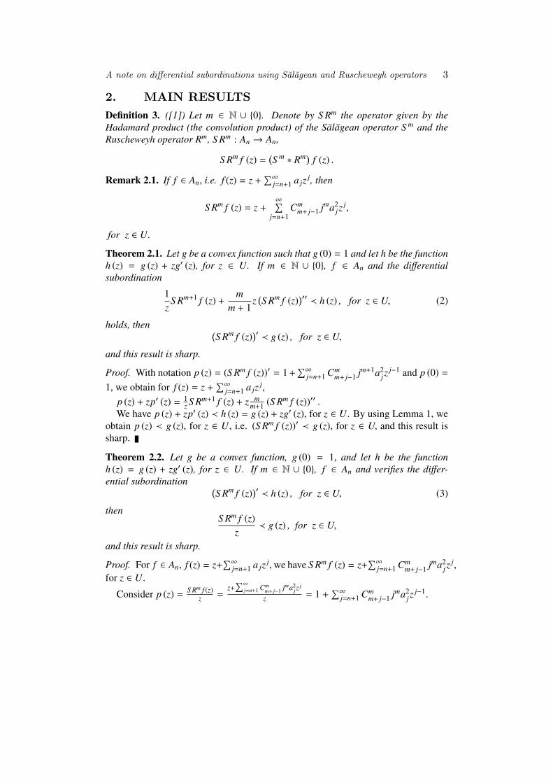
2. MAIN RESULTSDefinition 3. ([1]) Let m ∈ N ∪ 0. Denote by S Rm the operator given by theHadamard product (the convolution product) of the Salagean operator S m and theRuscheweyh operator Rm, S Rm : An → An,

S Rm f (z) =(S m ∗ Rm)

f (z) .

Remark 2.1. If f ∈ An, i.e. f (z) = z +∑∞

j=n+1 a jz j, then

S Rm f (z) = z +∞∑

j=n+1Cm

m+ j−1 jma2jz

j,

for z ∈ U.

Theorem 2.1. Let g be a convex function such that g (0) = 1 and let h be the functionh (z) = g (z) + zg′ (z), for z ∈ U. If m ∈ N ∪ 0, f ∈ An and the differentialsubordination

1z

S Rm+1 f (z) +m

m + 1z(S Rm f (z)

)′′ ≺ h (z) , for z ∈ U, (2)

holds, then (S Rm f (z)

)′ ≺ g (z) , for z ∈ U,


Proof. With notation p (z) = (S Rm f (z))′ = 1 +∑∞

j=n+1 Cmm+ j−1 jm+1a2

jzj−1 and p (0) =

1, we obtain for f (z) = z +∑∞

j=n+1 a jz j,

p (z) + zp′ (z) = 1z S Rm+1 f (z) + z m

m+1 (S Rm f (z))′′ .We have p (z) + zp′ (z) ≺ h (z) = g (z) + zg′ (z), for z ∈ U. By using Lemma 1, we

obtain p (z) ≺ g (z), for z ∈ U, i.e. (S Rm f (z))′ ≺ g (z), for z ∈ U, and this result issharp.

Theorem 2.2. Let g be a convex function, g (0) = 1, and let h be the functionh (z) = g (z) + zg′ (z), for z ∈ U. If m ∈ N ∪ 0, f ∈ An and verifies the differ-ential subordination (

S Rm f (z))′ ≺ h (z) , for z ∈ U, (3)

thenS Rm f (z)

z≺ g (z) , for z ∈ U,


Proof. For f ∈ An, f (z) = z+∑∞

j=n+1 a jz j,we have S Rm f (z) = z+∑∞

j=n+1 Cmm+ j−1 jma2

jzj,

for z ∈ U.

Consider p (z) =S Rm f (z)

z =z+∑∞


j zj

z = 1 +∑∞


jzj−1.

4 Alina Alb Lupas

We have p (z) + zp′ (z) = (S Rm f (z))′, for z ∈ U.Then (S Rm f (z))′ ≺ h (z), for z ∈ U, becomes p (z)+zp′ (z) ≺ h (z) = g (z)+zg′ (z),

for z ∈ U. By using Lemma 1, we obtain p (z) ≺ g (z), for z ∈ U, i.e. S Rm f (z)z ≺ g (z),

for z ∈ U.

Theorem 2.3. Let g be a convex function such that g (0) = 1 and let h be the functionh (z) = g (z) + zg′ (z), for z ∈ U. If m ∈ N ∪ 0, f ∈ An and verifies the differentialsubordination (

zS Rm+1 f (z)S Rm f (z)

)′≺ h (z) , for z ∈ U, (4)

thenS Rm+1 f (z)S Rm f (z)

≺ g (z) , for z ∈ U,


Proof. For f ∈ An, f (z) = z+∑∞

j=n+1 a jz j,we have S Rm f (z) = z+∑∞


jzj,

for z ∈ U.

Consider p (z) =S Rm+1 f (z)S Rm f (z) =

z+∑∞

j=n+1 Cm+1m+ j jm+1a2

j zj

z+∑∞


j zj

=1+

∑∞j=n+1 Cm+

m+ j jm+1a2j z

j−1

1+∑∞


j zj−1.

We have p′ (z) =(S Rm+1 f (z))′

S Rm f (z) − p (z) · (S Rm f (z))′S Rm f (z) .

Then p (z) + zp′ (z) =

(zS Rm+1 f (z)

S Rm f (z)

)′.

Relation (4) becomes p (z) + zp′ (z) ≺ h (z) = g (z) + zg′ (z), for z ∈ U, and by usingLemma 1, we obtain p (z) ≺ g (z), for z ∈ U, i.e. S Rm+1 f (z)

S Rm f (z) ≺ g (z), for z ∈ U.

References[1] A. Alb Lupas, Certain differential subordinations using Salagean and Ruscheweyh operators,

Mathematica (Cluj), Proceedings of International Conference on Complex Analysis and RelatedTopics, The 11th Romanian-Finnish Seminar, Alba Iulia, 2008 (to appear).

[2] S.S. Miller, P.T. Mocanu, Differential Subordinations. Theory and Applications, Marcel DekkerInc., New York, Basel, 2000.

[3] St. Ruscheweyh, New criteria for univalent functions, Proc. Amet. Math. Soc., 49(1975), 109-115.

[4] G. St. Salagean, Subclasses of univalent functions, Lecture Notes in Math., Springer Verlag,Berlin, 1013(1983), 362-372.

ON TOPOLOGICAL AG-GROUPOIDSAND PARAMEDIAL QUASIGROUPSWITH MULTIPLE IDENTITIES

ROMAI J., 6, 1(2010), 5–14

Natalia Bobeica, Liubomir ChiriacTiraspol State University, Chisinau, Republic of [email protected], [email protected]

Abstract This paper studies some properties of (n,m)-homogeneous isotopies of topological AG-groupoids and paramedial quasigroups with (n,m)-identities. We study properties ofparamedial groupoids with multiple identities. We extend some affirmations of the the-ory of topological groups on the class of topological (n,m)-homogeneous quasigroups.

Keywords: AG-groupoid, quasigroups, (n,m)-identity, (n,m)-homogeneous isotope.2000 MSC: 97U99.

1. INTRODUCTIONIn this work we study the (n,m)-homogeneous isotopies of AG-topological groupoid

with multiple identities and some topological properties of topological paramedialquasigroups.The results established in this paper are related to the results of M.Choban and L. Kiriyak in [2] and to the research papers [6-14]. In section 3 weexpand on the notions of multiple identities and (n,m)-homogeneous isotopies in-troduced in [5]. This concept facilitates the study of topological groupoids with(n,m)-identities. In this section we prove that if (G,+) is an AG-topological groupoidand e is an (1, p)-zero, then every (n, 1)-homogeneous isotope (G, ·) of (G,+) is anAG-groupoid, with (1, np)-identity e in (G, ·). In section 4 we study the paramedialgroupoids with multiple identities. We present some interesting properties of a classof paramedial groupoids with (2, 1)-identities. We prove that if P is an open compactset of a right identity of a topological right paramedial loop G, then P contains anopen compact topological right paramedial subloop Q. This result was obtained byL.S. Pontrjagin for topological groups in (Theorem 16, [13]) and by L.L. Chiriac fortopological left medial quasigroups in [14]. We shall use the notations and terminol-ogy from [1-3, 13].

2. BASIC NOTIONSA non-empty set G is said to be a groupoid relatively to a binary operation denoted

by “ · ”, if for every ordered pair (a, b) of elements of G there is a unique elementab = a · b ∈ G.

5

6 Natalia Bobeica, Liubomir Chiriac

If the groupoid G is a topological space and the binary operation (a, b) → a · b iscontinuous, then G is called a topological groupoid.

An element e ∈ G is called an identity if ex = xe = x for every x ∈ X.A quasigroup with an identity is called a loop. A groupoid G is called medial if it

satisfies the law xy · zt = xz · yt for all x, y, z, t ∈ G.A groupoid G is called paramedial if it satisfies the law xy · zt = ty · zx for all

x, y, z, t ∈ G.If a paramedial guasigroup G contains an element e such that e · x = x(x · e = x)

for all x in G, then e is called a left (right) identity element of G and G is called a left(right) paramedial loop.

A groupoid (G, ·) is called a groupoid Abel-Grassmann or AG-groupoid if it satis-fies the left invertive law (a · b) · c = (c · b) · a for all a, b, c ∈ G.

A groupoid G is said to be hexagonal if it is idempotent, medial and semisymetric,i.e. the equalities x · x = x, xy · zt = xz · yt, x · zx = xz · x = z hold for all of itselements. The last identities (semisymetric law) can be represented in the form of anequivalence x · z = t ⇔ x = z · t.

A groupoid G is called bicommutative if it satisfies the law xy · zt = tz · yx for allx, y, z, t ∈ G.

3. GROUPOIDS WITH MULTIPLE IDENTITIESConsider a groupoid (G,+). For every two elements a, b from (G,+) we denote:

1(a, b,+) = (a, b,+)1 = a + b, and n(a, b,+) = a + (n − 1)(a, b,+),(a, b,+)n = (a, b,+)(n − 1) + b

for all n ≥ 2.If a binary operation (+) is given on a set G, then we shall use the symbols n(a, b)

and (a, b)n instead of n(a, b,+) and (a, b,+)n.

Definition 3.1. Let (G,+) be a groupoid and let n,m ≥ 1. The element e of thegroupoid (G,+) is called:

- an (n,m)-zero of G if e + e = e and n(e, x) = (x, e)m = x for every x ∈ G;- an (n,∝)-zero if e + e = e and n(e, x) = x for every x ∈ G;- an (∝,m)-zero if e + e = e and (x, e)m = x for every x ∈ G.

Clearly, if e ∈ G is both an (n,∝)-zero and an (∝,m)-zero, then it is also an (n,m)-zero. If (G, ·) is a multiplicative groupoid, then the element e is called an (n,m)-identity. The notion of (n,m)-identity was introduced in [5].

Example 3.1. Let (G, ·) be a paramedial groupoid, e ∈ G and ex = x for every x ∈ G.Then (G, ·) is a paramedial groupoid with (1, 2)-identity e in G. Indeed, if x ∈ G, thenxe · e = xe · ee = ee · ex = e · ex = e · x = x.

Example 3.2. Let G = 1, 2, 3, 4, 5. We define the binary operation ” · ”:

On topological AG-groupoids and paramedial quasigroups with multiple identities 7

· 1 2 3 4 5

1 1 5 4 3 2

2 3 2 1 5 4

3 5 4 3 2 1

4 2 1 5 4 3

5 4 3 2 1 5

Then (G, ·) is a non-commutative, hexagonal and AG-quasigroup and each elementfrom (G, ·) is a (2, 4)-identity in G.

Definition 3.2. Let (G,+) be a topological groupoid. A groupoid (G, ·) is called ahomogeneous isotope of the topological groupoid (G,+) if there exist two topologicalautomorphisms ϕ, ψ : (G,+)→ (G,+) such that x · y = ϕ(x) + ψ(y), for all x, y ∈ G.

For every mapping f : X → X we denote f 1(x) = f (x) and f n+1(x) = f ( f n(x)) forany n ≥ 1.

Definition 3.3. Let n,m ≤ ∞. A groupoid (G, ·) is called an (n,m)-homogeneous isotope of a topological groupoid (G,+) if there exist two topologicalautomorphisms ϕ, ψ : (G,+)→ (G,+) such that:

1. x · y = ϕ(x) + ψ(y) for all x, y ∈ G;2. ϕψ = ψϕ;3. If n < ∞, then ϕn(x) = x for all x ∈ G;4. If m < ∞, then ψm(x) = x for all x ∈ G.

Definition 3.4. A groupoid (G, ·) is called an isotope of a topological groupoid(G,+), if there exist two homeomorphisms ϕ, ψ : (G,+) → (G,+) such that x · y =

ϕ(x) + ψ(y) for all x, y ∈ G.

Under the conditions of Definition 3.4 we shall say that the isotope (G, ·) is gen-erated by the homeomorphisms ϕ, ψ of the topological groupoids (G,+) and write(G, ·) = g(G,+, ϕ, ψ).

Example 3.3. Let (R,+) be the topological Abelian group of real numbers.1. If ϕ(x) = 5x, ψ(x) = x and x · y = 5x + y, then (R, ·) = g(R,+, ϕ, ψ) is a

locally compact medial quasigroup. By virtue of Theorem 7 from [2], there exists aleft invariant Haar measure on (R, ·).

2. If ϕ(x) = 5x, ψ(x) = 7x and x ·y = 5x + 7y, then (R, ·) = g(R,+, ϕ, ψ) is a locallycompact medial quasigroup and on (R, ·) as above, by virtue of Theorem 7 from [2],does not exist any left or right invariant Haar measure.

Example 3.4. Denote by Zp = Z/pZ = 0, 1, ..., p − 1 the cyclic Abelian group oforder p. Consider the commutative group (G,+) = (Z7,+), ϕ(x) = 3x, ψ(x) = 4x and


x ·y = 3x+4y. Then (G, ·) = g(G,+, ϕ, ψ) is a medial, paramedial and bicommutativequasigroup and the neutral element of (G,+) is a (3, 6)-identity in (G, ·).Example 3.5. Consider the commutative group (G,+) = (Z5,+), ϕ(x) = 3x, ψ(x) =

2x and x · y = 3x + 2y. Then (G, ·) = g(G,+, ϕ, ψ) is a medial, paramedial andbicommutative quasigroup and the neutral element of (G,+) is a (4, 4)-identity in(G, ·).Example 3.6. Consider the commutative group (G,+) = (Z7,+), ϕ(x) = 2x, ψ(x) =

5x and x · y = 2x + 5y. Then (G, ·) = g(G,+, ϕ, ψ) is a medial, paramedial andbicommutative quasigroup and the neutral element of (G,+) is a (6, 3)-identity in(G, ·).Example 3.7. Consider the commutative group (G,+) = (Z7,+), ϕ(x) = 3x, ψ(x) =

5x and x · y = 3x + 5y. Then (G, ·) = g(G,+, ϕ, ψ) is a medial and hexagonalquasigroup and each element of (G, ·) is a (6, 6)-identity.

Theorem 3.1. If (G,+) is an AG-groupoid and e ∈ G is an (1, p)-zero, then every(n, 1)-homogeneous isotope (G, ·) of the topological groupoid (G,+) is AG-groupoidwith (1, np)-identity e in (G, ·) and a + bc = b · (a + c) for all a, b, c ∈ G and n, p ∈ N.

Proof. We will prove that e is an (1, np)-identity in (G, ·) by the method described in[2]. Let (G, ·) be an (n, 1)-homogeneous isotope of the groupoid (G,+) and e be an(1, p)-zero in (G,+). We mention that ϕq(e) = ψq(e) = e for every q ∈ N. Then in(G,+) we have q · 1(e, x,+) = x for each x ∈ G and for every q ∈ N. Since we have(n, 1)-homogeneous isotope (G, ·) then m = 1 and ψ(x) = x for all x ∈ G. In this case

1(e, x, ·) = 1(e, ψ(x),+)

and

q(e, x, ·) = q(e, ψq(x),+)

for every q ≥ 1. Therefore

1(e, x, ·) = 1(e, ψ(x),+) = 1(e, x,+) = x.

Analogously we obtain that

(e, x, ·)np = (e, ϕnp(x),+)np = (e, x,+)np = x.

Hence e is an (1, np)-identity in (G, ·). The mediality of the AG-topological groupoid(G,+) follows from [4]. Really,

(x + y) + (z + t) = ((z + t) + y) + x = ((y + t) + z) + x = (x + z) + (y + t).


Since e is an (1, p)-zero in (G,+), hence e is left zero and e + x = x for everyx ∈ (G,+). In this case for each AG-groupoid (G,+) with (1, p)-zero we get

x + (z + t) = (e + x) + (z + t) = (e + z) + (x + t) = z + (x + t).

We will prove that (n, 1)-homogeneous isotope (G, ·) of the topologicalgroupoid (G,+) is AG-groupoid and x·(zt) = z·(xt). Since (G, ·) is (n, 1)-homogeneousisotope of (G,+), then ψ(x) = x. Hence

x · zt = ϕ(x) + ψ(zt) =

= ϕ(x) + zt = ϕ(x) + (ϕ(z) + ψ(t)) = ϕ(z) + (ϕ(x) + ψ(t)) =

= ϕ(z) + xt = ϕ(z) + ψ(xt) = z · xt.

Therefore the identity x · zt = z · xt holds in groupoid (G, ·). We will show thata + bc = b · (a + c). Really,

a + bc = (ea) + (bc) = (ϕ(e) + ψ(a)) + (ϕ(b) + ψ(c)) =

= (ϕ(e) + ϕ(b)) + (ψ(a) + ψ(c)) = ϕ(e + b) + ψ(a + c) =

= ϕ(b) + ψ(a + c) = b · (a + c).

The proof is complete.

Corollary 3.1. If (G,+) is an AG-groupoid and e is a left zero, then every (1, 1)-homogeneous isotope (G, ·) of the topological groupoid (G,+) is AG-groupoid withleft identity e in (G, ·) and a + bc = b · (a + c), for all a, b, c ∈ G.

4. SOME PROPERTIES OF PARAMEDIALQUASIGROUPS

We provide an example of a paramedial quasigroup which is not medial.

Example 4.1. Let G = 1, 2, 3, 4. We define the binary operation ” · ”:

· 1 2 3 4

1 2 1 3 4

2 3 4 2 1

3 4 3 1 2

4 1 2 4 3

Then (G, ·) is a paramedial quasigroup but it is not medial. Indeed, for example

(2 · 3) · (1 · 4) , (2 · 1) · (3 · 4).


Theorem 4.1. If (G, ·) is a multiplicative groupoid, e ∈ G and the following condi-tions hold:

1. xe = x for every x ∈ G,2. x2 = x · x = e for every x ∈ G,3. xy · z = xz · y for all x, y, z ∈ G,4. for every a, b ∈ G there exists an unique point y ∈ G such that ya = b,

then e is a (2, 1)-identity in G.

Proof. Fix x ∈ G. Pick y ∈ G such that y · ex = x. By conditions 2 of Theorem 4.1we have

(y · ex) · x = x · x = e. (1)

By condition 3 of this theorem

(y · ex) · x = yx · ex. (2)

From (1) and (2) we obtain

yx · ex = e. (3)

It is clear that

ex · ex = e. (4)

Thus, from (3) and (4)

yx · ex = ex · ex.

Hence yx = ex and y = e. Therefore y · (e · x) = e(ex) = x and e is a(2, 1)− identity in G. The proof is complete.


1. xe = x for every x ∈ G,2. x2 = x · x = e for every x ∈ G,3. x · zt = t · zx for all x, y, z ∈ G,4. for every a, b ∈ G there exists a unique point y ∈ G such that ya = b,

then e is a (2, 1)-identity in G.

Proof. Similar to Theorem 4.1.

Remark 4.1. The proofs of Theorems 4.1. and 4.2. are based on a rather generalmethod. Professor I. Burdujan noticed that there is an easier way to prove Theorem4.2. He observed that e · ex = x · ee = xe = x and e is a (2, 1)-identity in G.



1. xe = x for every x ∈ G,2. x2 = x · x = e for every x ∈ G,3. xy · uv = vy · ux for all x, y, u, v ∈ G,4. if xa = ya then x = y for all x, y, a ∈ G,

then (G, ·) is a paramedial quasigroup with a (2, 1)-identity e.

Proof. If x ∈ G, then

e · ex = ee · ex = xe · ee = xe · e = x · e = x.

Thus e is (2, 1)− identity. Consider the equation xa = b. Then

xa · e = b · e,xa · ee = be,ea · ex = be,

(ea · ex) · be = be · be.

Thus, (ea · ex) · (be) = e. By condition (3) of theorem 4.3 we have

(e · ex) · (b · ea) = e. (5)

From (5) we obtain

x · (b · ea) = e. (6)

By condition (2) of theorem 4.3

(b · ea) · (b · ea) = e. (7)

From (6) and (7) have x = b · ea. Since xa = b we can verify that (b · ea) · a =

(b · ea) · (ae) = (e · ea) · (ab) = a · ab = ae · ab = be · aa = be · e = b.In this case the element x = b ·ea is a unique solution of the equation xa = b. Now

we consider the equation ay = b. We have

e · b = e · ay = ee · ay = ye · ae = y · a.

Thus ya = eb and, by considering the solution of equation xa = b we have

y = eb · ea = ab · ee = ab · e = ab.

It follows that y = ab is a unique solution of the equation ay = b. The proof iscomplete.

Corollary 4.1. If (G, ·) is a paramedial quasigroup with a (2, 1)-identity e, then so-lutions of the equations xa = b and ay = b are respectively x = b · ea and y = ab forevery a, b ∈ G.

Lemma 4.1. Let P be a subset of topological right paramedial loop (G, ·) and e ∈ P.If P1 = P ∩ eP, then


1. eP1 = P1.2. If P is open, then P1 is open.3. If P is closed, then P1 is closed.4. If P is compact, then P1 is compact.

Proof. The mapping f : G → G, where f (x) = ex, is a homeomorphism and P1 =

P ∩ eP. That proved the assertions 2, 3 and 4. For every x ∈ G we have e · ex = x.Therefore, eP1 = eP ∩ (e · eP) = eP ∩ P = P1. The proof is complete.

Proposition 4.1. Let (G, ·) be a right paramedial loop. Then the mapping

f : G → G, where f (x) = ex,

is an involutive mapping, i.e. f = f −1.

Proof. It is obvious that f is an one-to-one mapping. The solution of a equationay = b is y = ab. Hence a · ab = b for every y ∈ G. In particular e · ex = x andf ( f (x)) = x. Hence f = f −1.The proof is complete.

Theorem 4.4. Let (G, ·) be a topological right paramedial loop with the identityx2 = e. If P is an open compact subset such that e ∈ P, then P contains an opencompact right paramedial subloop (Q, ·) of (G, ·).Proof. In virtue of Lemma 4.1 we consider that eP = P. Note Q = q ∈ G : qP∪Pq ⊂P. We prove that Q is an open compact right paramedial subloop. Now we show thatQ is the open set. Let q be a fixed point of Q and x be an arbitrary point of P. Sincexq ∈ P and P is an open set, then there exists such neighborhoods Ux 3 x and Vx 3 q,such that UxVx ⊂ P. In this case we have P =

⋃∞i=1 Uxi . Because P is a compact

set we can extract an open finitely subcovering Ux1 , ...,Uxk such that P =⋃k

i=1 Uxi .Note V =

⋂ki=1 Vxi . Then PV ⊂ P. Let us consider qx ∈ P. By analogy we prove that

there exists such neighborhood W 3 q so that WP ⊂ P. Note V ∩W = U. Then wehave that UP ⊂ P and PU ⊂ P. Hence for the open set U 3 q we have that U ⊂ Q.Therefore Q is the open set.

Let us show that Q is a closed set. Suppose that p < Q. Then for some q ∈ P wehave that pq < P or qp < P. Let us assume that pq < P. Then there exists an open setU such that p ∈ U and Uq ⊂ G \ P. Therefore U ∩ Q = ∅ and q is not a limit pointof a set Q. It follows that the set Q is closed.

We show that Q ⊂ P. If q ∈ Q, then q ∈ qP ∩ Pq. Since if qP ∪ Pq ⊂ P, thenq ∈ P. Therefore Q ⊂ P. By condition of theorem eP ∪ Pe = P ∪ P = P ⊂ P. Hencee ∈ Q.

We will prove that Q is a right paramedial loop. Fix a, b ∈ Q. Then

P · ab = Pe · ab = be · aP = b · aP = b · P ⊂ P


and

ab · P = ab · eP = Pb · ea = P · ea = Pe · ea = ae · eP = a · P ⊂ P.

Therefore ab ∈ Q and Q is a subgroupoid of G. If a, b ∈ Q then for equation xa = bhis solution x = b · (ea) is in Q. Really, since e, a ∈ Q we have ea ∈ Q, and b · ea ∈ Q.For equation ay = b his solution y = ab is also in Q. Hence Q is a right paramedialsubloop of G. The proof is complete.

Theorem 4.5. Let (G, ·) be a topological paramedial quasigroup with a (2, 1)-identitye and x2 = e for every x ∈ G. If P is an open compact subset from G such thate ∈ P, then P contains an open compact paramedial subquasigroup (Q, ·) with a(2, 1)-identity e.

Proof. It follows from Theorem 4.3, Lemma 4.1 and Theorem 4.4. The proof iscomplete.

Remark 4.2. For topological groups a series of properties that are based on thenotion of open compact are proved (see[3, 13]).

5. SOME REMARKS OF MEDIALQUASIGROUPS

The ideas used in the proofs of Theorem 4.3, Lemma 4.1, Theorem 4.4 can beadopted for topological right medial loops. We mention the following properties.

Remark 5.1. If (G, ·) is a right medial loop, then the mapping f : G → G, wheref (x) = ex, is an involutive automorphism, i.e. f = f −1 and f (x · y) = f (x) · f (y) forevery x, y ∈ G.

Remark 5.2. If (G, ·) is a right medial loop, e ∈ G and x2 = e for every x ∈ G, thene is a (2, 1)-identity.

Remark 5.3. Let (G, ·) be a right medial loop and x2 = e for every x ∈ G. Therelated operation x y = ex · ey in G satisfies the following properties:1. (G, ) is a medial quasigroup.2. e x = x for every x ∈ G.3. H = x ∈ G : ex = x is a commutative group and is a subloop of the loops (G, ·)and (G, ).Example 5.1. Let (G,+) be a commutative group. We define in G the operation ” · ”:x · y = x − y for every x, y ∈ G. Then (G, ·) is a right medial loop and the identityelement e of (G,+) is a (2, 1)-identity for it.

Acknowledgements. The authors gratefully acknowledge helpful suggestions ofthe referees.


References[1] V. D. Belousov, Foundation of the theory of quasigroups and loops, Moscow, Nauka, 1967.

[2] M. M. Choban, L. L. Kiriyak, The topological quasigroups with multiple identities, Quasigroupsand Related Systems, 9(2002), 19-31.

[3] E. Hewitt, K. A. Ross, Abstract harmonic analysis, Vol. 1: Structure of topological groups. Inte-gration theory. Group representation, Springer-Verlag, Berlin-Gottingen-Heidelberg, 1963.

[4] M. A. Kazim, M. Naseeruddin, On almost-semigroups, Aligarh Bulletin of Mathematics, AligarhMuslim Univ., Aligarh, India, 8(1978), 67-70.

[5] M. M. Choban, L. L. Kiriyak, The Medial Topological Quasigroup with Multiple identities, The4 th Conference on Applied and Industrial Mathematics, Oradea-CAIM, 1995, p.11.

[6] L. L. Chiriac, On Topological Quasigroups and Homogeneous Isotopies, Analele Universitatiidin Pitesti, Buletin Stiintific, Seria Matematica si Informatica, 9(2003), 191-196.

[7] L. L. Chiriac, N. Bobeica, Some properties of the homogeneous isotopies, Acta et Commenta-tiones, Universitatea de Stat Tiraspol, Chisinau, 3(2006), 107-112.

[8] L. L. Chiriac, N. Bobeica, Paramedial topological groupoids, 6th Congress of Romanian Mathe-maticians, Bucharest, Romania, June 28-July 4, 2007, 25-26.

[9] L. L. Chiriac, L. Chiriac Jr, N. Bobeica, On topological groupoids and multiple identities, Bulet-inul Academiei de Stiinte a RM, Matematica, 1(59)(2009), 67-78.

[10] L. L. Chiriac, Topological paramedial groupoids with multiple identities, The 17-th Conferenceon Applied and Industrial Mathem., Constantza-CAIM, Romania, 2009, p. 28.

[11] N. Bobeica, On Paramedial Loops, The 17-th Conference on Applied and Industrial Mathem.,Constantza-CAIM, Romania, 2009, p. 20.

[12] N. Bobeica, Topological Hexagonal Groupoids with Multiple Identities, MITRE-2009, State Uni-versity of Moldova, October, 2009, 5-6.

[13] L. S. Pontrjagin, Neprerivnie gruppi, Nauka, Moskow, 1984.

[14] L. L. Chiriac, Topological Algebraic System, Stiinta, Chisinau, 2009.

AUTOMORPHISMS AND DERIVATIONSOF HOMOGENEOUS QUADRATICDIFFERENTIAL SYSTEMS

ROMAI J., 6, 1(2010), 15–28

Ilie BurdujanDepartment of Mathematics, University of Agricultural and Veterinary Medicine”Ion Ionescu de la Brad” Iasi, Romaniaburdujan [email protected]

Abstract A binary algebra is associated with any homogeneous quadratic differential system.Derivations and automorphisms of a homogeneous quadratic differential system are justderivations and automorphisms of the algebra associated to it. The real 3-dimensionalcommutative algebras without nilpotent elements of order two, which have a derivation,are classified up to an isomorphism. Consequently, the corresponding homogeneousquadratic differential systems are classified up to a center-affine equivalence.

Keywords: homogeneous quadratic differential system.2000 MSC: 37C99.

1. INTRODUCTIONThe theory of quadratic differential system (shortly, QDS) is the first step toward

a systematic study of nonlinear systems of differential equations. There exist almostexhaustive studies on QDSs with two unknown functions [8], [5], [13], [14]. Moreexactly, the classification up to an affine equivalence of these systems was achieved.In fact, several classifications were made according with various classification cri-teria. Among them we quote the classifications which were achieved by Markus[8] (with a completion due to Date [5]) and those due to Vulpe-Sibirschii [13] forquadratic differential systems in plane.

Unfortunately, the similar studies for similar systems in R3 creates important tech-nical difficulties. A direction which had opened large perspectives for the study ofsystems of quadratic differential equations (and, more general, of systems of polyno-mial differential equations) was the one revealed by L. Markus [8] in 1960. Markusrealized that a commutative algebra, which may be a non-associative one (in gen-eral), can be naturally associated to each homogeneous quadratic differential system(shortly, HQDS). Along this way, the homogeneous quadratic differential systemscan be studied on the multidimensional spaces and on Banach spaces as well.

The derivations and the automorphisms of a HQDS (i.e. of the quadratic vectorform which defines it) are defined. The existence of such automorphisms entails theexistence of certain symmetries that - in their turn - imply the existence of some

15

16 Ilie Burdujan

suitable coordinates in which the system would take the simplest form (i.e., a largenumber of system’s coefficients would be either 0 or ”small” integers). Notice thatany derivation (resp. automorphism) of a HQDS is a derivation (resp. automorphism)of its associated algebra.

In the first part of this paper we present several results concerning the HQDSson Banach spaces. They generalize the similar results that were already proved forHQDSs on Rn (see, for example, [6], [7], [9], [14]). The last part of our paper dealswith the classification of some HQDSs on R3. To this end, we firstly remark thatthe set of important general results, concerning the derivation algebra of a real com-mutative algebra, is not too large. However, there exist notable progresses on thissubject for the so-called NN-algebras, i.e. algebras without nilpotent elements of or-der 2 (see [1], [2]). Some results concerning the derivation algebra of an NN-algebraare presented and they are used for classifying the real 3-dimensional commutativeNN-algebras having at least a derivation. It was proved that there exist nine multi-parametric classes of nonisomorphic such NN-algebras. Accordingly, there exist ninemultiparametric classes of HQDSs onR3, whose associated algebras are NN-algebraswith a derivation, that are mutually nonequivalent up to an affinity.

2. PRELIMINARIESLet E(‖ · ‖1) be a real Banach space.

Definition 2.1. Any equation of the form

dXdt

= F(X) (1)

where F : E → E is a continuous quadratic vector form on E is called a homoge-neous quadratic differential equation (shortly, HQDE) on E.

Recall that a vector form F is quadratic if F(sX) = s2F(X) for all s ∈ R and X ∈ E.With any quadratic vector form F is associated its polar form which is a symmetricbilinear vector form G : E × E → E defined by

G(X,Y) =12

[F(X + Y) − F(X) − F(Y)] , (2)

for all X,Y ∈ E. The definition of tensor product assures us that there exists a uniquelinear mapping µF : E ⊗ E → E such that µ ιE = G (here ιE(x, y) = x ⊗ y). In itsturn, µF is naturally identified with a (1,2)-tensor. Since G is symmetric, it resultsthat µF is a covariant symmetric (1,2)-tensor.

On the other hand, G allows to define a commutative binary operation ”·” on E by

x · y = G(x, y) for all x, y ∈ E. (3)

The obtained commutative algebra is denoted by E(·). In general, E(·) is a non-associative algebra. Taking into account that x · x = x2 = F(x), HQDE (1) can be

Automorphisms and derivations of homogeneous quadratic differential systems 17

written in the formdXdt

= X2, (4)

for pointing out its connection with algebra E(·).Now, let us consider another HQDE on the real Banach space E′, namely

dYdt

= F1(Y), (5)

where F1 : E′ → E′ is a continuous quadratic vector form. The polar form G1 of F1can be identified with a covariant symmetric (1,2)-tensor on E′. The binary operation” ∗ ”, defined on E′ by

x ∗ y = G1(x, y) for all x, y ∈ E, (6)

organizes E′ as a commutative algebra denoted by E′(∗).Definition 2.2. It is said that HQDE (1) is center-affinely equivalent (or, CA-equiva-lent) with the HQDE (5) if and only if there exists a continuously invertible linearmapping h : E′ → E such that X = h(Y) is a solution for (1) whenever Y is a solutionfor (5); in this case it is said that h is an equivalence of equation (1) with equation(5). An equivalence of equation (1) with itself is called an automorphism of equation(1) or an automorphism of F.

Proposition 2.1. [3] HQDE (1) is CA-equivalent with the HQDE (5) if and only ifthere exists a continuously invertible linear mapping h : E′ → E such that

h F1 = F h. (7)

Since h−1 is continuous and the equality h−1 F = F1 h−1 holds, it results thefollowing assertion.

Corolar 2.1. If (1) is CA-equivalent with (5), then (5) is also CA-equivalent with (1).

Theorem 2.1. [3] Equations (1) and (5) are CA-equivalent if and only if the algebrasE(·) and E′(∗) are continuously isomorphic. The continuous linear mapping h : E →E is an automorphism for (1) if and only if it is a continuous automorphism of algebraE(·).

If Φt and Ψt denote the flows of equations (1) and (5), respectively, then the twoequations are CA-equivalent if and only if there exists a continuous invertible linearmapping h : E′ → E such that

h Ψt = Φt h.

Remark 2.1. The existence of a CA-equivalence h : E′ → E allows to identify thespaces E′ and E. Then, Theorem 2.1 assures us that there exists a 1-to-1 correspon-dence between the set of classes of CA-equivalent HQDEs on E and the set of classes

18 Ilie Burdujan

of isomorphic commutative algebras defined on E. Accordingly, there exists a corre-spondence between certain qualitative properties of a HQDE (1) and the propertiesinvariant up to an isomorphism of the associated algebra.

Remark 2.2. The binary CA-equivalence relation defined by Definition 2.2 on theset of HQDEs on a fixed Banach space is an equivalence relation (i.e. it is reflex-ive, symmetric and transitive). That is why, in what follows, we shall use the termequivalence instead of CA-equivalence.

Theorem 2.1 assures us that there exists a correspondence between the affinelyinvariant properties of any HQDE and the properties invariant up to an isomorphismof the associated algebra. This correspondence is not completely identified. Some ofits components are presented in the next Proposition.

Proposition 2.2. The following assertions hold, for any HQDE (1) on the Banachspace E:

1. the set N(E) of all nilpotents of order two of E(·) is in a bijective correspondencewith the set of all steady state solutions of (1),

2. the set I(E) of all idempotents of E(·) is in a bijective correspondence with theset of ray (from or to 0) solutions of (1),

3. E(·) is a nilalgebra if and only if all solutions of (1) are polynomials,4. E2 = E · E is a proper ideal of E if and only if (1) has at least a linear prime

integral,5. if E(·) is a power-associative algebra then all solutions of (1) are rational

functions.

In fact, any structural property of E(·) (i.e., a property which is invariant up to anisomorphism) enforces the existence of a property of Eq. (1) (and conversely). Forexample, if E(·) has no idempotent element then the zero solution of (1) is not asymp-totically stable; if (1) has a Liapunov function then E has no idempotent element.

NOTE. These results were already proved, in the finite dimensional case, byKinyon&Sagle, Rorhl, Walcher (see [6], [9], [14]).

3. DERIVATIONS AND AUTOMORPHISMS OFA HQDS

Definition 3.1. A derivative of F is any continuous linear transformation D : E → Esatisfying

DF(X) = F′(X) · DX f or all X ∈ E, (8)

where F′(X) · Y = lims→0

dF(X + sY)ds f or all X, Y ∈ E. Any derivative of the vector

form F is also named a derivation of HQDE (1).


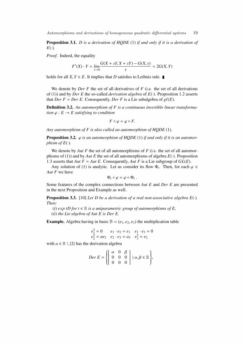
Proposition 3.1. D is a derivation of HQDE (1) if and only if it is a derivation ofE(·).Proof. Indeed, the equality

F′(X) · Y = lims→0

G(X + sY, X + sY) −G(X, y)s

= 2G(X, Y)

holds for all X,Y ∈ E. It implies that D satisfies to Leibniz rule.

We denote by Der F the set of all derivatives of F (i.e. the set of all derivationsof (1)) and by Der E the so-called derivation algebra of E(·). Proposition 1.2 assertsthat Der F = Der E. Consequently, Der F is a Lie subalgebra of g`(E).

Definition 3.2. An automorphism of F is a continuous invertible linear transforma-tion ϕ : E → E satisfying to condition

F ϕ = ϕ F.

Any automorphism of F is also called an automorphism of HQDE (1).

Proposition 3.2. ϕ is an automorphism of HQDE (1) if and only if it is an automor-phism of E(·).

We denote by Aut F the set of all automorphisms of F (i.e. the set of all automor-phisms of (1)) and by Aut E the set of all automorphisms of algebra E(·). Proposition1.3 asserts that Aut F = Aut E. Consequently, Aut F is a Lie subgroup of GL(E).

Any solution of (1) is analytic. Let us consider its flow Φt. Then, for each ϕ ∈Aut F we have

Φt ϕ = ϕ Φt .

Some features of the complex connections between Aut E and Der E are presentedin the next Proposition and Example as well.

Proposition 3.3. [10] Let D be a derivation of a real non-associative algebra E(·).Then:

(i) exp tD for t ∈ R is a uniparametric group of automorphisms of E,(ii) the Lie algebra of Aut E is Der E.

Example. Algebra having in basis B = (e1, e2, e3) the multiplication table

e21 = 0 e1 · e2 = e1 e1 · e3 = 0

e22 = ae2 e2 · e3 = a3 e2

3 = e2

with a ∈ R \ 2 has the derivation algebra

Der E =

α 0 β0 0 00 0 0

| α, β ∈ R,

20 Ilie Burdujan

and the automorphism group

Aut E =

α 0 β0 1 00 0 ±1

| α, β ∈ R, α , 0

.

4. THE CLASSIFICATION OF REAL3-DIMENSIONAL NN-ALGEBRAS WITHDERIVATIONS

In [2], [3] it was proved that any real 3-dimensional NN-algebra A(·) hasdim Der A ∈ 0, 1 and that there exist NN-algebras having a derivation. Conse-quently, the problem to classify, up to an isomorphism, the real 3-dimensional NN-algebras having derivations is consistent.

Let A(·) be a real 3-dimensional NN-algebra with a nonzero derivation. Then thereexists a derivation D with the eigenvalues 0,±i ([1], [2]). Accordingly, there existsa basis B = (e1, e2, e3) such that

De1 = 0, De2 = −e3, De3 = e2, e22 = e2

3, e2 · e3 = 0.

In fact, the natural vector space decomposition A = ker D ⊕ Im D exists. Sinceker D is a 1-dimensional NN-algebra, it contains an idempotent element e1. Then,the equalities De2

2 = −2e2 · e3 = 0 imply e22 = e2

3 = εe1 with ε , 0. We can choose e2and e3 such that ε = ±1. Supposing now that e1 · e2 = ae1 + be2 + ce3 and applyingD to it, it follows e1 · e3 = −ce2 + be3. Applying again D to e1 · e3 it results thate1 · e2 = be2 + ce3. Therefore, the multiplication table of the algebra, in basis B, is

T e21 = e1 e1 · e2 = be2 + ce3 e1 · e3 = −ce2 + be3

e22 = εe1 e2

3 = εe1 e2 · e3 = 0,

where either ε = ±1, b2 + c2 , 0 or ε = 1, b = c = 0 (these conditions assure that Ais an NN-algebra).

We shall denote by A(b, c, ε) the algebra having, in a basis B, the multiplicationtable T.

In order to classify, up to an isomorphism, the real 3-dimensional NN-algebraswe need to identify the lattices of their subalgebras. First at all, we determinethe idempotents of such algebras, because they identify all the 1-dimensional sub-algebras. We denote by I(A) the set of all idempotents of A(·). The condition(xe1 + ye2 + ze3)2 = xe1 + ye2 + ze3 is equivalent to the system

x2 + ε(y2 + z2) = x(2bx − 1)y − 2cxz = 02cxy + (2bx − 1)z = 0.

(9)


Obviously, this last homogeneous system has the null solution, which is not of anyinterest in the problem of idempotents; since e1 is an idempotent, the system (4) hasnecessarily the solution x = 1, y = z = 0. It remains to look for the solutions withx < 0, 1 and y2 + z2 , 0. In this case, necessarily

∆ =

∣∣∣∣∣∣2bx − 1 −2cx

2cx 2bx − 1

∣∣∣∣∣∣ = (2bx − 1)2 + 4c2x2 = 0,

i.e. b , 0, x =1

2b , c = 0. This time, system (4) has solutions only when k =

ε2b − 1

4b2 > 0, namely:

x =12b, y =

√k cos θ, z =

√k sin θ for θ ∈ [0, 2π).

Therefore, the following four classes of real 3-dimensional NN-algebras arise natu-rally:

C1. A(b, c, ε) with c , 0,C2. A(b, 0, ε) with b , 0, and k ≤ 0,C3. A(b, 0, ε) with b , 0, and k > 0,C4. A(0, 0, 1).

The following assertions are readily provable:

• if A belongs to class C1, then I(A) = e1 and Le1 has the eigenvalues 1, b ± ic,• if A belongs to class C2, then I(A) = e1 and Le1 has the eigenvalues 1, b, b,• if A belongs to class C3, then

I(A) = e1 ∪ e(b) =1

2be1 +

√k(e2 cos θ + e3 sin θ) | θ ∈ [0, 2π), b , 0;

Le1 has the eigenvalues 1, b, b and Le(b) has the eigenvalues1, 1

2 ,1 − b

2b

,

• algebra A(0, 0, ε) has I(A) = e1 and Le1 has the eigenvalues 1, 0, 0.Taking into account the idempotents and their spectra it results that the four classes

C1, C2, C3, C4 provide a partition of the set of all real 3-dimensional NN-algebraswith a derivation. Anyone of these classes can be separately analysed for being pos-sibly partitioned in subclasses of non-isomorphic algebras.

Proposition 4.1. The set of algebras belonging to class C1 have the properties:

(i) Algebras A(b, c, ε) and A(b,−c, ε), (with c , 0), are always isomorphic,(ii) Algebras A(b, c, ε) and A(b′, c′, ε), with c > 0 and c′ > 0, are isomorphic if

and only if b = b′ and c = c′.(iii) Any two algebras A(b, c, 1) and A(b′, c′,−1) with c > 0 and c′ > 0 are non-

isomorphic.

22 Ilie Burdujan

Proof. (i) It is enough to consider the multiplication table of A(b, c, ε) in basis B′ =

( f1 = e1, f2 = e2, f3 = −e3).(ii) If T : A(b, c, ε)→ A(b′, c′, ε) is an isomorphism, then necessarily T (e1) = f1. Ase1 and f1 must have the same spectrum it results b′ = b and c′ = c.(iii) Let us suppose that A(b, c, 1) has, in basis B, the multiplication table T whileA(b′, c′,−1) has, in basis B′ = ( f1, f2, f3), the multiplication table

T’ f 21 = f1 f1 · f2 = b′ f2 + c′ f3 f1 · f3 = −c′ f2 + b′ f3

f 22 = − f1 f 2

3 = − f1 f2 · f3 = 0.

If T : A(b, c, ε) → A(b′, c′,−ε) is an isomorphism, then necessarily T (e1) = f1 anda′ = a, b′ = b. If T (e2) = α f1 +β f2 +γ f3, then T (e2

2) = T (e1) = (T (e2))2 is equivalentto

α2 − β2 − γ2 = 1bαβ − cαγ = 0cαβ + bαγ = 0.

The last two equations imply αβ = αγ = 0. Since the first equation excludes thepossibility α = 0, the condition α , 0 implies β = γ = 0 and T (αe1 − e2) = 0 (whatcontradicts the injectivity of T ).

In a similar way it is proved the following Proposition.

Proposition 4.2. The set of algebras belonging to classes C2 and C3 have the prop-erties:

(i) Algebras A(b, 0, ε) and A(b′, 0, ε) with bb′ , 0 are isomorphic if and only ifb = b′.

(ii) Any two algebras A(b, 0, 1) and A(b′, 0,−1) with bb′ , 0 are not isomorphic.

Therefore, these results give the classification up to an isomorphism of the real3-dimensional NN-algebras which have a nonzero derivation. More exactly, it wasobtained the following result.

Theorem 4.1. If A(·) is a real 3-dimensional commutative NN-algebra which has anonzero derivation, then there exists a basis in A such that its multiplication tablehas the form corresponding to one of the following nine classes of non-isomorphicalgebras:

1 A(b, c, 1) with b, c ∈ R and c > 0,2 A(b, c,−1) with b, c ∈ R and c > 0,3 A(b, 0, 1) with b ∈ R, b , 0 and b ≤ 1

2 ,

4 A(b, 0,−1) with b ∈ R \ 1 and b ≥ 12 ,

5 A(b, 0, 1) with b ∈ R \ 1 and b > 12 ,

6 A(b, 0,−1) with b ∈ R, b , 0 and b < 12 ,


7 A(1, 0, 1),8 A(1, 0,−1),9 A(0, 0, 1).

Proposition 4.3. Every algebra A(b, c, ε), with b2 + c2 , 0, is simple.

Proof. Let I ⊂ A be a nonzero ideal and v = xe1 + ye2 + ze3 ∈ I, v , 0; then theelements

v · e1 = xe1 + (by − cz)e2 + (cy + bz)e3,v · e2 = εye1 + bxe2 + cxe3,v · e3 = εze1 − cxe2 + bxe3,

belong to I. Consequently, if ∆ = x(b2 + c2)[x2 − ε(y2 + z2)] is nonzero then v · e1,v · e2 and v · e3 are linearly independent and, necessarily, I ≡ A. If x = 0, then theequalities v · e2 = εye1, v · e3 = εze1 and v , 0 imply e1, e1 · e2, e1 · e3 ∈ I, i.e.I ≡ A. In the case when x , 0 and ax2 − ε(y2 + z2) = 0, the linear independenceof vectors v · e2, v · e3 and (v · e2) · e3 = εcxe1 + εy(−ce2 + be3)(∈ I) is equivalentto condition ∆1 = εx(b2 + c2)[cx2 − εyz] , 0; similarly, the linear independenceof vectors v · e2, v · e3 and (v · e3) · e2 = −εcxe1 + εz(be2 + ce3)(∈ I) is equivalentto condition ∆2 = −εx(b2 + c2)[cx2 + εyz] , 0. Therefore, if ∆2

1 + ∆22 , 0 then

I ≡ A. If ∆21 + ∆2

2 = 0, then cx2 = εyz = 0 imply necessarily c = 0 and b , 0.Thus, the complementary cases y = 0 and, respectively, y , 0 must be considered.When y = 0 (necessarily, c = 0 and b , 0), then e2 =

1bxv · e2 ∈ I, e1 · e2 ∈ I and

e1 =1εbx (v · e2) · e2 ∈ I, e1 · e3 ∈ I, i.e. I ≡ A. In its turn, y , 0 implies z = 0,

i.e. v = xe1 + ye2. Then e3 =1bxv · e3 ∈ I, e1 · e3 ∈ I and e1 =

1εbx (v · e3) · e3 ∈ I,

e1 · e3 ∈ I, i.e. I ≡ A.

NOTE. If b = c = 0 then A2 = Re1 is a nontrivial ideal.

Proposition 4.4. The algebras A(1, 0, ε) are unitary and power-associative as well.

According to Theorem 4.2.2 [3], Der A = RD. Therefore, etD | t ∈ R is a uni-parametric group of automorphisms for A(·); it is isomorphic to the matrix group

1 0 00 cos θ − sin θ0 sin θ cos θ

∣∣∣∣∣∣∣∣θ ∈ [0, 2π)

. Certainly, Aut A do not contain other uni-

parametric subgroup of automorphisms. The problem is to establish whether othernew automorphisms of A(·) exist or do not exist. The answer is contained in the nextProposition.

Proposition 4.5. Aut A coincides with the matrix group

1 0 00 cos θ − sin θ0 sin θ cos θ

∣∣∣∣∣∣∣∣θ ∈ [0, 2π)

.

24 Ilie Burdujan

Recall that the trace form of algebra A(·) is the bilinear form g : A×A→ R definedby

g(v,w) = trace Lv·w for all v,w ∈ A.

Let us consider v = x1e1 + x2e2 + x3e3 and w = y1e1 + y2e2 + y3e3 in A. Since

Lv =

x1 εx2 εx3

bx2 − cx3 bx1 −cx1cx2 + bx3 cx1 bx1

,

v · w = [x1y1 + ε(x2y2 + x3y3)]e1 + [b(x1y2 + x2y1) − c(x1y3 + x3y1)]e2 + [c(x1y2 +

x2y1) + b(x1y3 + x3y1)]e3 and trace Lv = (2b + 1)x1,it results that

g(v,w) = (2b + 1)[x1y1 + ε(x2y2 + x3y3)].

This bilinear form vanishes identically when b = −1/2 and it is nondegenerate when-ever b , −1/2.

In what follows we try to solve the HQDSs corresponding to these NN-algebras.The before presented results assures that, for a HQDS with three unknown functionswhose associated algebra is an NN-algebra with a nonzero derivation, which belongsto class C1, there exists a change of variables (i.e., of unknown functions) such thatthe system becomes

dx1dt = x2

1 + ε(x22 + x2

3)dx2dt = 2bx1x2 − 2cx1x3

dx3dt = 2cx1x2 + 2bx1x3

(10)

with ε = ±1 and b, c ∈ R and c > 0. The next equation is obtained adding the lasttwo equations, after their multiplication with x2 and respectively x3,

d(x22 + x2

3)dt

= 4bx1(x22 + x2

3). (11)

Using the change of unknown functions y2 = x22 + x2

3, z2 =x2x3

, the system (5)becomes

dx1dt = x2

1 + εy2

dy2dt = 4bx1y2

dz2dt = −2cx1(1 + z2

2).

(12)

This last system allows us to determine the following independent prime integrals for


(5):

f1(x1, x2, x3) = ln(2b

x21

x22 + x2

3+

2bε1 − 2b

)− 1 − 2b

2b · ln(x2

2 + x23

),

f2(x1, x2, x3) = c · ln(x2

2 + x23

)+ 2b · arctg x2

x3

if b < 0, 1/2. In the case b = 0, c > 0, ε = 1 the system (5) has the following twoindependent prime integrals:

f1(x1, x2, x3) = x22 + x2

3,

f2(t, x1, x2, x3) =1√

x22 + x2

3

· arctg x1√x2

2 + x23

− t.

If b = 0, c > 0, ε = −1 then the system (5) has the following two independent primeintegrals:

f1(x1, x2, x3) = x22 + x2

3,

f2(t, x1, x2, x3) =1

2(x22 + x2

3)· ln

x1 −√

x22 + x2

3

x1 +

√x2

2 + x23

− t.

In case b = 1/2, c > 0, ε = 1, system (5) has the following prime integrals:

f1(x1, x2, x3) = c ln (x22 + x2

3) + arctg x2x3,

f2(x1, x2, x3) = (x22 + x2

3) e

x21

x22 + x2

3 .

Finally, in the case b = 1/2, c > 0, ε = −1 the system (5) has the following twoindependent prime integrals:

f1(x1, x2, x3) = c ln(x22 + x2

3) + arctg x2x3,

f2(x1, x2, x3) =x2

1x2

2 + x23

+ ln(x22 + x2

3).

The HQDS corresponding to an algebra of type C2 or C3 has the form

dx1dt = x2

1 + ε(x22 + x2

3)dx2dt = 2bx1x2

dx3dt = 2bx1x3.

(13)

It has the following two independent prime integrals:

f1(x1, x2, x3) =x2x3,

f2(x1, x2, x3) =[(1 − 2b)x2

1 + ε(x22 + x2

3)]

x−1/b3 .

26 Ilie Burdujan

Let us solve the Cauchy problem with the initial data x1(0) = α, x2(0) = β,x3(0) = γ.

Considering the complex function z = x2 + ix3, the last two equations in (5) leadsto

dzdt

= 2(b + ic)x1z.

A straightforward computation gives us

x2(t) = ke2bθ(t)cos (2cθ(t) + ϕ0)x3(t) = ke2bθ(t)sin (2cθ(t) + ϕ0)

where ϕ0 = arctg γβ

, k2 = β2 + γ2 and θ(t) =∫ t

0 x1(τ) dτ.In its turn, the equation (6) gives

x22 + x2

3 = k2e4bθ(t).

Therefore, the first equation in (5) may be transformed into the following integro-differential equation:

dx1

dt= x2

1 + εk2e4bθ(t). (14)

Differentiating (14), it follows

d2x1

dt2 − 2(1 + 2b)x1dx1

dt+ 4bx3

1 = 0. (15)

In the case b , 0, this nonlinear equation can be analysed by the method of Liesymmetries. System (5) can be solved in the case b = 0. Indeed, for ε = 1, theCauchy problem, with the initial data x1(0) = α, x2(0) = β, x3(0) = γ, has thesolution

x1(t) = k ksin kt + αcos ktkcos kt − αsin kt

x2(t) = k cos (2cθ(t) + ϕ0)x3(t) = k sin (2cθ(t) + ϕ0)

(16)

where θ(t) = −1k ln |a sin kt − k cos kt|. In the case ε = −1, the solution is

x1(t) = k k sinh kt + α cosh ktk cosh kt − α sinh kt

x2(t) = k cos (2cθ(t) + ϕ0)x3(t) = k sin (2cθ(t) + ϕ0),

(17)


where

θ(t) = −(1 +

αk

) ln∣∣∣∣∣tanh

kx2− 1

∣∣∣∣∣k − α −

(1 − αk

) ln∣∣∣∣∣tanh

kx2

+ 1∣∣∣∣∣

k + α+

+(α2

k + k)

ln

∣∣∣∣∣∣∣k tanh(kx2

)2

− 2a tanhkx2

+ k

∣∣∣∣∣∣∣(k + α)(k − α) − (k2 + α2) ln k

k(k2 − α2).

According to Proposition 1.3 [7], the orbit etD(P) of P is a solution to HQDS (5)if and only if P is a nonzero solution of equation P2 = DP.

Let us find the solution of HQDS (5) that are orbits of the Lie group Aut A. IfP = α e1 + β e2 + γ e3, then the equation P2 = DP becomes

α2 + ε(β2 + γ2) = 02bαβ − 2cαγ = −γ2cαβ + 2bαγ = β.

(18)

Equation (18) has a nonzero solution when ε = −1, only. Any such a solution musthave α , 0. Therefore, the last two equations in (18) can be written in the form

2bα β − (2cα − 1)γ = 0(2cα − 1)β + 2bα γ = 0.

This homogeneous system, with the unknowns β and γ, has a nonzero solution if andonly if ∣∣∣∣∣∣

2bα −(2cα − 1)2cα − 1 2bα

∣∣∣∣∣∣ = 0⇔ 4b2α2 + (2cα − 1)2 = 0.

Therefore, the solutions P to DP = P2

in A(·) lie in the plane x1 = − 12c on the circle

with center (− 12c , 0, 0) and radius R =

∣∣∣∣∣−12c

∣∣∣∣∣. More exactly, they are

P(ω) = − 12c

e1 + R[e2 cos ω + e2 sin ω].

Then, the solution which is the trajectory through P(ω) is

Xω(t) = etDP(ω) = − 12c

e1 + R[e2 cos (t + ω) + e3 sin (t + ω)].

It is a periodic solution of the least period 2π. Moreover, Xω(t) is isolated in the setof all periodic solutions with period 2π.

Following Kinyon& Sagle [6], let us denote by S 1(c) and S 2(c) the sets S 1(c) =

v |trace Lv = c and S 2(c) = v |trace Lv2 = c, respectively. Then, the solution etDP

28 Ilie Burdujan

is on the plane S 1(c), where c = trace LP. Moreover, any periodic solution lies onS 1(c) ∩ S 2(0), what agrees with Proposition 5.23 [6].

NOTE. Equation (15) is of the form d2x1dt2 + f (x1)dx1

dt + g(x1) = 0 which contains

as particular cases van der Pol’s equation and Duffing’s equation, as well. We shallstudy it in a forthcoming paper.

References[1] B G., Osborn M. J., The derivation algebra of a real division algebra, Amer. J. of Math.,

103, 6(1981), 1135–1150.

[2] B I., On derivation algebra of a real algebra without nilpotents of order two, Ital. J. ofPure and Applied Math., 8(2000), 137–154.

[3] B I., Quadratic differential systems, 2008, Ed. PIM-Iasi. (in Romanian)

[4] B I., Infinitesimal groups associated with quadratic dynamical systems, ROMAI Journal,1, 1(2005), 37–42.

[5] D T., Classifications and Analysis of Two-dimensional Real Homogeneous Quadratic Differ-ential Equation Systems, J. Diff. Eqs., 32(1979), 311–334.

[6] K K. M., S A. A., Quadratic Dynamical Systems and Algebras, J. of Diff. Eqs,117(1995), 67–127 .

[7] K K. M., S A. A., Automorphisms and Derivations of Differential Equations and Alge-bras, Rocky Mountain J. of Math., 24, 1(1994), 135–153.

[8] M L., Quadratic Differential Equations and Non-associative Algebras, in ”Contributions tothe Theory of Nonlinear Oscillations”, Annals of Mathematics Studies, 45, Princeton UniversityPress, Princeton, N. Y., 1960.

[9] R H., Algebras and differential equations, Nagoya Math. J., 68(1977), 59–122.

[10] S, A. A., W, R. E., Introduction to L groups and L algebras, Academic Press, NewYork and London, 1973.

[11] S, D, Algebraic particular integrals, integrability and the problem of the center,Trans. A.M.S., 338(1979), 799–841.

[12] S, D, Basic Algebro-Geometric concepts in the study of planar polynomial vectorfields, Publicacions Mathematiques, 41(1997), 269–295.

[13] V, N. I.,Sı, K. S., Geometrical Classification of Quadratic differential systems , Dif-ferentialnye Uravnenje, 13, 5(1977), 803–814. (in Russian)

[14] W, S., Algebras and differential equations, Hadronic Press, Palm Harbor, 1991.

ON RADII OF STARLIKENESS ANDCLOSE-TO-CONVEXITY OF A SUBCLASSOF ANALYTIC FUNCTIONSWITH NEGATIVE COEFFICIENTS

ROMAI J., 6, 1(2010), 29–40

Adriana CatasFaculty of Sciences, University of Oradea, [email protected]

Abstract By making use of a multiplier transformation, a subclass of p-valent functions in theopen unit disc is introduced. The main results of the present paper provide various inter-esting properties of functions belonging to the new subclass. Some of these propertiesinclude, for example, several coefficient inequalities and distortion bounds for the func-tion class which is considered here. Relevant connections of some of the results obtainedin this paper with those in earlier works are also provided.

Keywords: analytic function, multiplier transformations, coefficient inequalities, distortion bounds,radii of starlikeness and close-to-convexity.2000 MSC: 30C45.

1. PRELIMINARIESLet H be the class of analytic functions in the open unit disc

U = z ∈ C : |z| < 1

and H[a, n] be the subclass of H consisting of functions of the form f (z) = a+anzn +

an+1zn+1 + · · · . Let A(p, n) denote the class of normalized functions f (z) of the form

f (z) = zp +

∞∑

k=p+n

akzk, (p, n ∈ N := 1, 2, 3, . . . ) (1)

which are analytic in the open unit disc. In particular, we set

A(p, 1) := Ap and A(1, 1) := A = A1.

For two functions f (z) given by (1) and g(z) given by

g(z) = zp +

∞∑

k=p+n

bkzk, (p, n ∈ N) (2)

29

30 Adriana Catas

the Hadamard product (or convolution) ( f ∗ g)(z) is defined, as usual, by

( f ∗ g)(z) := zp +

∞∑

k=p+n

akbkzk := (g ∗ f )(z). (3)

Definition 1.1. [3] Let f ∈ A(p, n). For δ ∈ R, δ ≥ 0, l ≥ 0, we define the multipliertransformations Ip(δ, l) on A(p, n) by the following infinite series

Ip(δ, l) f (z) := zp +

∞∑

k=p+n

[k + lp + l

]δakzk. (4)

It follows from (4) that

(p + l)Ip(δ + 1, l) f (z) = l · Ip(δ, l) f (z) + z(Ip(δ, l) f (z))′. (5)

If f is given by (1) then we have

Ip(δ, l) f (z) = ( f ∗ ϕδp,l)(z), (6)

where

ϕδp,l(z) = zp +

∞∑

k=p+n

[k + lp + l

]δzk. (7)

Let T(n, p) denote the class of functions f (z) of the form

f (z) = zp −∞∑

k=n+p

akzk, ak ≥ 0, p, n ∈ N, (8)

which are analytic in the open unit disc.Let A(n) be the class of functions of the form

f (z) = z −∞∑

k=n+1

akzk, ak ≥ 0, n ∈ N,

which are analytic in the open unit disc. Let S∗n(α) denote the subclass of A(n) con-sisting of functions which satisfy

Re(z f ′(z)f (z)

)> α, z ∈ U, 0 ≤ α < 1.

A function f (z), in S∗n(α) is said to be starlike of order α in U.A function f (z) ∈ A(n) is said to be convex of order α if it satisfies

Re(1 +

z f ′′(z)f ′(z)

)> α, z ∈ U, 0 ≤ α < 1.

On radii of starlikeness and close-to-convexity of a subclass of analytic functions... 31

Let Cn(α) be the subclass of A(n) consisting of all convex of order α functions [2].We denote by S∗n(p, α) and Cn(p, α) the classes of p-valently starlike functions of

order α in U, 0 ≤ α α, z ∈ U, 0 ≤ α α, z ∈ U, 0 ≤ α < p

. (10)

An interesting unification of the function classes S∗n(p, α) and Cn(p, α) is providedby the class Tn(p, α, γ) of functions f (z) ∈ T(n, p), which also satisfy the followinginequality

Re(

z f ′(z) + γz2 f ′′(z)γz f ′(z) + (1 − γ) f (z)

)> α, z ∈ U, 0 ≤ α < p, 0 ≤ γ ≤ 1. (11)

The class Tn(p, α, γ) was investigated by Alintas et al. [1].

2. COEFFICIENT INEQUALITIESIn this section we will define a new class of p-valently starlike functions by using

the multiplier transformations Ip(m, l), m ∈ N, l ≥ 0 as in (4) and we will establishcertain coefficient inequalities relating to the new introduced class.

Definition 2.1. Let 0 ≤ α < p, 0 ≤ γ ≤ 1, m ∈ N, l ≥ 0, p ∈ N∗. A function fbelonging to T(n, p) is said to be in the class Tm

l (n, p, α, γ) if and only if

Re

(1 − γ)z(Ip(m, l) f (z))′ + γz(Ip(m + 1, l) f (z))′

(1 − γ)z(Ip(m, l) f (z)) + γz(Ip(m + 1, l) f (z))

> α, z ∈ U. (12)

Remark 2.1. The class Tml (n, p, α, γ) is a generalization of the subclasses

i) T00(1, 1, α, 0) ≡ T∗(α) ≡ S∗1(α) and T1

0(1, 1, α, 0) ≡ C(α) ≡ C1(α) defined andstudied by Silverman [6];

ii) T00(n, 1, α, 0) and T1

0(n, 1, α, 0) studied by Chatterjea [4] and Srivastava et al.[7];

iii) Tm0 (n, p, α, γ) studied by Kamali [5].

Theorem 2.1. Let the function f be defined by (8). Then f belongs to the classTm

l (n, p, α, γ) if and only if

∞∑

k=n+p

cp,k(m, l)(k − α)[p + l + γ(k − p)]ak ≤ (p + l)(p − α). (13)

32 Adriana Catas

where

cp,k(m, l) =

[k + lp + l

]m

. (14)

The result is sharp and the extremal functions are

fk(z) = zp − (p + l)(p − α)cp,k(m, l)(k − α)[p + l + γ(k − p)]

· zk, k ≥ n + p. (15)

Proof. Assume that the inequality (4) holds and let |z| = 1. Then we have∣∣∣∣∣∣(1 − γ)z(Ip(m, l) f (z))′ + γz(Ip(m + 1, l) f (z))′

(1 − γ)z(Ip(m, l) f (z)) + γz(Ip(m + 1, l) f (z))− p

∣∣∣∣∣∣ =

=

∣∣∣∣∣∣∣∣∣∣∣∣∣∣∣

∞∑

k=n+p

[k + lp + l

]m [p + l + γ(k − p)

p + l

](k − p)akzk−p

1 −∞∑

k=n+p

[k + lp + l

]m [p + l + γ(k − p)

p + l

]akzk−p

∣∣∣∣∣∣∣∣∣∣∣∣∣∣∣

≤ p +

∞∑

k=n+p

[k + lp + l

]m [p + l + γ(k − p)

p + l

]kak − p

1 −∞∑

k=n+p

[k + lp + l

]m [p + l + γ(k − p)

p + l

]ak

≤ p − α.

Consequently, by the maximum modulus theorem one obtains

f (z) ∈ Tml (n, p, α, γ).

Conversely, suppose that f (z) ∈ Tml (n, p, α, γ). Then from (4) we find that

Re

pzp −∞∑

k=n+p

[k + lp + l

]m [p + l + γ(k − p)

p + l

]kakzk

zp −∞∑

k=n+p

[k + lp + l

]m [p + l + γ(k − p)

p + l

]akzk

> α.

Choose values of z on the real axis such that

(1 − γ)z(Ip(m, l) f (z))′ + γz(Ip(m + 1, l) f (z))′

(1 − γ)z(Ip(m, l) f (z)) + γz(Ip(m + 1, l) f (z))


is real. Letting z→ 1− through real values, we obtain

Re

p −∞∑

k=n+p

[k + lp + l

]m [p + l + γ(k − p)

p + l

]kak

1 −∞∑

k=n+p

[k + lp + l

]m [p + l + γ(k − p)

p + l

]ak

≥ α

or, equivalently

p −∞∑

k=n+p

[k + lp + l

]m [p + l + γ(k − p)

p + l

]kak

≥ α1 −

∞∑

k=n+p

[k + lp + l

]m [p + l + γ(k − p)

p + l

]ak

which gives (27).

Theorem 2.2. Let the function f defined by (8) be in the class Tml (n, p, α, γ). Then

∞∑

k=n+p

ak ≤ (p + l)(p − α)cp,n+p(m, l)(p + l + γn)(n + p − α)

(16)

and∞∑

k=n+p

kak ≤ (p + l)(p − α)(n + p)cp,n+p(m, l)(p + l + γn)(n + p − α)

. (17)

The equality in (16) and (17) is attained for the function f given by (15).

Proof. By using Theorem 2.1, we find from (4) that

(p + l + γn)(n + p − α)cp,n+p(m, l)∞∑

k=n+p

ak

≤∞∑

k=n+p

cp,k(m, l)(k − α)[p + l + γ(k − p)]ak ≤ (p + l)(p − α),

which immediately yields the first assertion (16) of Theorem 2.2.On the other hand, taking into account the inequality (4), we also have

(p + l + γn)cp,n+p(m, l)∞∑

k=n+p

(k − α)ak ≤ (p + l)(p − α)

34 Adriana Catas

that is

(p + l + γn)cp,n+p(m, l)∞∑

k=n+p

kak

≤ (p + l)(p − α) + α(p + l + γn)cp,n+p(m, l)∞∑

k=n+p

ak

which, in view of the coefficient inequality (16), can be put in the form

(p + l + γn)cp,n+p(m, l)∞∑

k=n+p

kak

≤ (p + l)(p − α) + α(p + l + γn)cp,n+p(m, l)(p + l)(p − α)

cp,n+p(m, l)(p + l + γn)(n + p − α)

and this completes the proof of (17).

3. DISTORTION THEOREMSTheorem 3.1. Let the function f defined by (8) be in the class Tm

l (n, p, α, γ). Thenwe have

|Ip(i, l) f (z)| ≥ |z|p − (p + l)(p − α)cp,k(m − i, l)(n + p − α)(p + l + γn)

· |z|n+p (18)

and

|Ip(i, l) f (z)| ≤ |z|p +(p + l)(p − α)

cp,k(m − i, l)(n + p − α)(p + l + γn)· |z|n+p (19)

for z ∈ U, where 0 ≤ i ≤ m and cp,k(m − i, l) is given by (14).The equalities in (5) and (6) are attained for the function f given by

fn+p(z) = zp − (p − α)(p + l)m+1

(p + n + l)m(n + p − α)(p + l + γn)zn+p. (20)

Proof. Note that f ∈ Tml (n, p, α, γ) if and only if Ip(i, l) f (z) ∈ Tm−i

l (n, p, α, γ), where

Ip(i, l) f (z) = zp −∞∑

k=n+p

cp,k(i, l)akzk. (21)

By Theorem 2.1, we know that

cp,k(m − i, l)(n + p − α)(p + l + γn)∞∑

k=n+p

cp,k(i, l)ak ≤


≤∞∑

k=n+p

cp,k(m, l)(k − α)[p + l + γ(k − p)]ak ≤ (p + l)(p − α)

that is∞∑

k=n+p

cp,k(i, l)ak ≤ (p + l)(p − α)cp,k(m − i, l)(n + p − α)(p + l + γn)

. (22)

The assertions of (5) and (6) of Theorem 3.1 follow immediately. Finally, we notethat the equalities (5) and (6) are attained for the function f defined by

Ip(i, l) f (z) = zp − (p + l)(p − α)cp,k(m − i, l)(n + p − α)(p + l + γn)

zn+p. (23)

This completes the proof of Theorem 3.1.

Corollary 3.1. Let the function f defined by (8) be in the class Tml (n, p, α, γ). Then

we have

| f (z)| ≥ |z|p − (p + l)(p − α)cp,k(m, l)(n + p − α)(p + l + γn)

|z|n+p (24)

and

| f (z)| ≤ |z|p +(p + l)(p − α)

cp,k(m, l)(n + p − α)(p + l + γn)|z|n+p (25)

for z ∈ U. The equalities in (24) and (25) are attained for the function fn+p given in(7).


we have

| f ′(z)| ≥ p|z|p−1 − (p + l)(p − α)(n + p)cp,k(m, l)(n + p − α)(p + l + γn)

|z|n+p−1 (26)

and

| f ′(z)| ≤ p|z|p−1 +(p + l)(p − α)(n + p)

cp,k(m, l)(n + p − α)(p + l + γn)|z|n+p−1 (27)

for z ∈ U. The equalities in (26) and (27) are attained for the function fn+p given in(7).


the unit disc is mapped onto a domain that contains the disc

|w| < cp,k(m, l)(n + p − α)(p + l + γn) − (p + l)(p − α)cp,k(m, l)(n + p − α)(p + l + γn)

. (28)

The result is sharp with the extremal function fn+p given in (7).

36 Adriana Catas

4. CLOSURE THEOREMSLet the functions fi be defined for i = 1, 2, . . . , s, by

fi(z) = zp −∞∑

k=n+p

ak,izk, ak,i ≥ 0, n, p ∈ N, z ∈ U. (29)

We shall prove the following results for the closure of the class Tml (n, p, α, γ).

Theorem 4.1. Let the functions fi defined by (8) be in the class Tml (n, p, α, γ), for

every i = 1, 2, . . . , s. Then the functions h defined by

h(z) =

s∑

i=1

di fi(z), di ≥ 0 (30)

is also in the same class Tml (n, p, α, γ) if

m∑

i=1

di = 1. (31)

Proof. According to the definition of h, we can write

h(z) = zp −∞∑

k=n+p

s∑

i=1

diak,i

zk.

Further, since fi are in the class Tml (n, p, α, γ) for every i = 1, 2, . . . , s we get

∞∑

k=n+p

cp,k(m, l)(k − α)[p + l + γ(k − p)]ak,i ≤ (p + l)(p − α),

where cp,k(m, l) is given by (28).Hence we can see that

∞∑

k=n+p

cp,k(m, l)(k − α)[p + l + γ(k − p)]

s∑

i=1

diak,i

=

=

s∑

i=1

di

∞∑

k=n+p

cp,k(m, l)(k − α)[p + l + γ(k − p)]ak,i

≤

≤ (p + l)(p − α)s∑

i=1

di = (p + l)(p − α),

which implies that h is in the class Tml (n, p, α, γ).


Corollary 4.1. The class Tml (n, p, α, γ) is closed under a convex linear combination.

Proof. Let the function fi, i = 1, 2, be in the class Tml (n, p, α, γ). It is sufficient to

show that the function h defined by

h(z) = µ f1(z) + (1 − µ) f2(z), 0 ≤ µ ≤ 1 (32)

is in the class Tml (n, p, α, γ). But, taking s = 2, d1 = µ and d2 = 1 − µ in Theorem

4.1, one obtains that Tml (n, p, α, γ) is a convex set.

Remark 4.1. As a consequence of Theorem 4.1, there exist the extreme points of theclass T j(n, γ, α, λ).

Theorem 4.2. Let fk be defined as in (15), k ≥ n + p and

fn+p−1 = zp, z ∈ U. (33)

Then f is in the class Tml (n, p, α, γ) if and only if it can be expressed in the form

f (z) =

∞∑

k=n+p−1

µk fk(z) (34)

where µk ≥ 0 (k ≥ n + p − 1) and∞∑

k=n+p−1

µk = 1.

Proof. Suppose that f can be expressed as in (34), namely

f (z) = zp −∞∑

k=n+p

µk(p + l)(p − α)

cp,k(m, l)(k − α)[p + l + γ(k − p)]· zk.

Then it follows that∞∑

k=n+p

cp,k(m, l)(k − α)[p + l + γ(k − p)]×

× (p + l)(p − α)cp,k(m, l)(k − α)[p + l + γ(k − p)]

=

= (p + l)(p − α)∞∑

k=n+p

µk ≤ (p + l)(p − α)

and by Theorem 2.1, f belongs to the class Tml (n, p, α, γ).

Conversely, assume that the function f belongs to the class Tml (n, p, α, γ). Then

∞∑

k=n+p

cp,k(m, l)(k − α)[p + l + γ(k − p)](p + l)(p − α)

ak ≤ 1.

38 Adriana Catas

We denote by

µk =cp,k(m, l)(k − α)[p + l + γ(k − p)]

(p + l)(p − α)ak, k ≥ n + p

and

µn+p−1 = 1 −∞∑

k=n+p

µk.

We notice that f can be expressed in the form (34). This completes the proof ofTheorem 4.2.

Corollary 4.2. The extrem points of the class Tml (n, p, α, γ) are the functions fk, k ≥

n + p, n, p ∈ N given by Theorem 4.2.

5. RADII OF CLOSE-TO-CONVEXITY,STARLIKENESS AND CONVEXITY

Theorem 5.1. Let the function f defined by (8) be in the class Tml (n, p, α, γ). Then f

is close-to-convex of order δ (0 ≤ δ < p), hence univalent, in the disc |z| < r1, where

r1 = infk

[(p − δ)cp,k(m, l)(k − α)[p + l + γ(k − p)]

(p + l)(p − α)k

] 1k−p

, k ≥ n + p. (35)

The result is sharp with the extremal function f given by (15).

Proof. It is sufficient to show that∣∣∣∣ f ′(z)

zp−1 − p∣∣∣∣ ≤ p − δ, |z| < r1 where r1 is given by

(35). From (8) we have

∣∣∣∣∣f ′(z)zp−1 − p

∣∣∣∣∣ ≤∞∑

k=n+p

kak|z|k−p.

Thus∣∣∣∣ f ′(z)

zp−1 − p∣∣∣∣ ≤ p − δ if

∞∑

k=n+p

(k

p − δ)

ak|z|k−p < 1. (36)

But Theorem 2.1 confirms that∞∑

k=n+p


ak ≤ 1, (37)

where cp,k(m, l) is given by (28).


Hence (36) will be true if(

kp − δ

)|z|k−p <


.

That is

|z| <[(p − δ)cp,k(m, l)(k − α)[p + l + γ(k − p)]

(p + l)(p − α)k

] 1k−p

. (38)

Theorem 5.1 follows easily from (38).

Theorem 5.2. Let the function f defined by (8) be in the class Tml (n, p, α, γ). Then f

is starlike of order δ, 0 ≤ δ < p, hence univalent, in the disc |z| < r2 where

r2 = infk

[(p − δ)cp,k(m, l)(k − α)[p + l + γ(k − p)]

(p + l)(p − α)(k − δ)] 1

k−p

, k ≥ n + p. (39)

The result is sharp with the extremal function f given by (15).

Proof. It is sufficient to show that∣∣∣∣ z f ′(z)

f (z) − p∣∣∣∣ < p − δ, |z| < r2 where r2 is given in

(39).If f is given by (8), then

∣∣∣∣∣z f ′(z)f (z)

− p∣∣∣∣∣ ≤

∞∑

k=n+p

(k − p)ak|z|k−p

1 −∞∑

k=n+p

ak|z|k−p

.

Thus,∞∑

k=n+p

k − δp − δak|z|k−p < 1. (40)

Hence, by using (37), the inequality (40) will be true if

|z| <[(p − δ)cp,k(m, l)(k − α)[p + l + γ(k − p)]

(p + l)(p − α)(k − δ)] 1

k−p

. (41)

and this completes the proof of Theorem 5.2.


f is convex of order δ, 0 ≤ δ < p (hence f is univalent), in the disc |z| < r3 where

r3 ≤ infk

[p(p − δ)cp,k(m, l)(k − α)[p + l + γ(k − p)]

k(p + l)(p − α)(k − δ)] 1

k−p

, k ≥ n + p. (42)

and cp,k(m, l) is given by (14), k ≥ n + p.

40 Adriana Catas

References[1] Alintas, O., Irmak, H., Srivastava, H.M., Fractional calculus and certain starlike functions with

negative coefficietns, Comput. Math. Appl., 30(2)(1995), 9-15.

[2] Alintas, O., Owa, S., Neighborhoods of certain analytic functions with negative coefficient, In-ternat. J. Math. and Math. Sci., 19(1996), 797-800.

[3] Catas, A., On certain class of p-valent functions defined by new multiplier transformations, Pro-ceedings Book of the International Symposium on Geometric Function Theory and Applications,August 20-24, 2007, TC Istanbul Kultur University, Turkey, 241-250.

[4] Chatterjea, S.K., On starlike functions, J. Pure Math., 1(1981), 23-26.

[5] Kamali, M., Neighborhoods of a new class of p-valently functions with negative coefficients,Math. Ineq. Appl., 9, 4(2006), 661-670.

[6] Silverman, H., Univalent functions with negative coefficients, Proc. Amer. Math. Soc., 51(1975),109-116.

[7] Srivastava, H.M., Owa, S., Chatterjea, S.K., A note on certain classes of starlike functions, Rend.Sem. Mat. Univ. Padova, 77(1987), 115-124.

PROXIMAL POINT METHODSFOR VARIATIONAL INEQUALITIESINVOLVING REGULAR MAPPINGS

ROMAI J., 6, 1(2010), 41–45

Corina L. ChiriacDepartment of Mathematics, Bioterra University, Bucharest, [email protected]

Abstract In this paper we consider the following general version of the proximal point algorithmfor solving a variational inequality, namely: find x ∈ C such that

〈F(x), u − x〉 ≥ 0

for all u ∈ C,where F : X → X∗, X is a Banach space with its dual X∗ and C ⊂ X anonempty, closed, convex set. First, choose any sequence of functions fn : X → X∗ thatare Lipschitz continuous. Then pick an initial element x0 and find xn+1 ∈ C such that

fn(xn+1 − xn) + F(xn+1) + NC(xn+1) 3 0 for n = 0, 1, 2, ...

where NC is the normal cone mapping of C. We prove that if the Lipschitz constant offn is bounded by half the reciprocal of the modulus of regularity of F + NC , then thereexists a neighborhood V of x (x being a solution of the variational inequality) such thatfor each initial point x0 ∈ V one can find a sequence xn generated by the algorithmwhich is linearly convergent to x.

Keywords: variational inequality, proximal point algorithm, regular mappings.2000 MSC: 47J20, 47J25, 58C30.

1. INTRODUCTIONIn this paper we study the convergence of a general version of the proximal point

algorithm for solving the variational inequality problem: find x ∈ C such

〈F(x), u − x〉 ≥ 0 (1)

for all u ∈ C, where F : X → X∗, X is a Banach space with its dual X∗ and C ⊂ Xa nonempty closed and convex set. Choose a sequence of functions fn : X → X∗with fn(0) = 0 and consider the following algorithm: given x0 find a sequence xn byapplying the iteration

fn(xn+1 − xn) + F(xn+1) + NC(xn+1) 3 0 (2)

for n = 0, 1, 2, ... .We prove in this work that if x is a solution of (1) and the mapping T = F + NC is

41

42 Corina L. Chiriac

metrically regular at x for 0 and with locally closed graph near (x, 0), then, for anysequence of functions fn that are Lipschitz continuous in a neighborhood U of theorigin, the same for all n, and whose Lipschitz constants ln have supremum that isbounded by half the reciprocal of the modulus of regularity of T, there exists a neigh-borhood V of x such that for each initial point x0 ∈ V one can find a sequencee xnsatisfying (2) which is linearly convergent to x in the norm of X.

If fn(x) = αnx and fn : X → X, we obtain the classical proximal point algorithmapplied for solving variational inequality

αn(xn+1 − xn) + T (xn+1) 3 0 (3)

for n = 0, 1, 2, ...proposed by Rockafellar [6] for the case when X is a Hilbert space and F is a mono-tone mapping. In particular, Rockafellar (see [6], Proposition 3) showed that whenxn+1 is an approximate solution of (3) and F is maximal monotone, then for a se-quence of positive scalars αn the iteration (3) produces a sequence xn which is weaklyconvergent to a solution to (1) for any starting point x0 ∈ C.

In the last thirty years a number of authors have studied generalizations of theproximal point algorithm with applications to specific variational inequalities. Wemention here the papers by Solodov and Svaiter [7], Auslender and Teboulle [1], Ka-plan and Tichatschke [5].

In this paper we consider the proximal point method, by employing recent de-velopments on regularity properties of mappings most of which can be found in thepaper [4].

In Section 2 we present some background material on metric regularity. Section 3gives a statement and a proof of the convergence result.

2. METRIC REGULARITYLet X and Y be Banach spaces, let G be a set-valued mapping G : X → 2Y and let

(x, y) ∈ gphG. Here gphG = (x, y) ∈ X × Y |y ∈ G(x) is the graph of G. We denoteby d(x,K) the distance from a point x to a set K, that is, d(x,K) = in fy∈K ‖x − y‖.Br(z) denotes the closed ball of radius r centered at z and G−1 is the inverse of Gdefined as x ∈ G−1(y)⇔ y ∈ G(x).

Definition 2.1. The mapping G is said to be metrically regular at x for y if thereexists a constant k > 0 such that

d(x,G−1(y)) ≤ kd(y,G(x)), for all (x, y) close to (x, y). (4)

The infimum of k for which (2.1) holds is the regularity modulus denoted reg G(x|y).

The case when G is not metrically regular at x for y corresponds to regG(x|y) = ∞.

Proximal point methods for variational inequalities involving regular mappings 43

An important result in the theory of metric regularity is the Lyusternik-Gravestheorem that says that the metric regularity is stable under perturbations of orderhigher than one.

Definition 2.2. A set K ⊂ X is locally closed at z ∈ K if there exists a > 0 such thatthe set K ∩ Ba(z) is closed.

Theorem 2.1. (Lyusternik-Graves [3]) Consider a mapping G : X → 2Y and any(x, y) ∈ gphG at which gphG is locally closed. Consider also a function g : X → Ywhich is Lipschitz continuous near x with a Lipschitz constant δ.If regG(x|y) < k < ∞ and δ < k−1, then

reg(g + G)(x|g(x) + y) ≤ (k−1 − δ)−1.

In the proof of our main result we used the following set-valued generalization ofthe Banach fixed point theorem.

Theorem 2.2. [2] Let (X, ρ) be a complete metric space, and consider a set-valuedmapping Φ : X → 2X , a point x ∈ X, and nonnnegative scalars α and θ be suchthat 0 ≤ θ < 1, the sets Φ(x) ∩ Ba(x) are closed for all x ∈ Ba(x) and the followingconditions hold:(i) d(x,Φ(x)) < α(1 − γθ);(ii) e(Φ(u) ∩ Ba(x),Φ(v)) ≤ θρ(u, v) for all u, v ∈ Ba(x).

Then Φ has a fixed point in Ba(x), that is, there exists x ∈ Ba(x) such that x ∈ Φ(x).

In the above, e(A, B) = supx∈Ad(x, B).

3. CONVERGENCE OF THE PROXIMAL POINTALGORITHM

Here we present the proof of our main result.We observe that the variational inequality problem (1.1) is equivalent to the prob-

lem: finding x ∈ X such that

0 ∈ F(x) + NC(x)

where NC : X → 2X∗ is the normal cone mapping, given by

NC(x) =y ∈ X∗ | for every x′ ∈ C, 〈x′ − x, y〉 ≤ 0

if x ∈ C; NC(x) = ∅ if x < C.

Theorem 3.1. Consider a mapping T = F + NC and let x be a solution of the vari-ational inequality (1.1). Let gphT be locally closed at (x, 0) and let T be metricallyregular at x for 0. Choose a sequence of functions fn : X → X∗ with fn(0) = 0 whichare Lipschitz continuous in a neighborhood U of 0, the same for all n, with Lipschitzconstants ln satisfying

supn

ln <1

2regT (x|0). (5)

44 Corina L. Chiriac

Then there exists a neighborhood V of x such that for any x0 ∈ V there exists a se-quence xn generated by the proximal point algorithm (2) which is linearly convergentto x.

Proof. Let l = supnln, then from (5) there exists k > regT (x|0) such thatkl < 0.5. Then one can choose λ which satisfies ((kl)−1 − 1)−1 < λ < 1.

Let r be such that the mapping T is metrically regular at x for 0 with a constant kand neighborhoods Br(x), B2lr(0) and B2r(0) ⊂ U.

Let x0 ∈ Br(x) ∩C. For any x ∈ Br(x) we have

‖− f0(x − x0)‖ = ‖ f0(x − x0) − f0(0)‖ ≤ l0 ‖x0 − x‖ ≤ 2rl0 ≤ 2lr.

We will show that the mapping Φ0(x) = T−1(− f0(x − x0)) satisfies the assumptionsof the fixed-point result in Theorem 2.2. First, by using the assumptions that T ismetrically regular at x for 0, 0 ∈ T (x) and f0(0) = 0, we have

d(x,Φ0(x)) = d(x,T−1(− f0(x − x0))) ≤ kd(− f0(x − x0), T (x)) ≤k ‖ f0(0) − f0(x − x0)‖ ≤ kl0 ‖x0 − x‖ ≤ kl0r < r(1 − kl0).

For any u, v ∈ Br(x), by the metric regularity of T,

e(Φ0(u) ∩ Br(x) ∩C,Φ0(v)) = supx∈T−1(− f0(u−x0))∩Br(x)

d(x,T−1(− f0(v − x0))) ≤sup

x∈T−1(− f0(u−x0))∩Br(x)kd(− f0(v − x0), T (x)) ≤ k ‖− f0(u − x0) − (− f0(v − x0))‖ ≤

kl0 ‖u − v‖.Hence there exists a fixed point x1 ∈ Φ0(x1) ∩ Br(x) ∩C,

x1 ∈ Br(x) ∩C and 0 ∈ f0(x1 − x0) + T (x1). (6)

If x1 = x there is nothing more to prove. Assume x1 , x. For any x ∈ Br(x), we have‖− f1(x − x1)‖ ≤ 2l1r ≤ 2lr. Now, we set

r1 = λ ‖x1 − x‖ . (7)

Since λ < 1 we have r1 < r. Consider the mapping Φ1(x) = T−1(− f1(x − x1)).By (7) and the metric regularity of T

d(x,Φ1(x)) = d(x,T−1(− f1(x − x1))) ≤ kd(− f1(x − x1), T (x)) ≤k ‖ f1(0) − f1(x − x1)‖ ≤ kl1 ‖x1 − x‖ < r1(1 − kl1).

For any u, v ∈ Br1(x), by the metric regularity of T, we obtain

e(Φ1(u) ∩ Br(x) ∩C,Φ1(v)) = supx∈T−1(− f1(u−x1))∩Br(x)

d(x,T−1(− f1(v − x1))) ≤

≤ supx∈T−1(− f1(u−x1))∩Br(x)

kd(− f1(v − x1),T (x)) ≤

Proximal point methods for variational inequalities involving regular mappings 45

≤ k ‖− f1(u − x1) − (− f1(v − x1))‖ ≤ kl1 ‖u − v‖ .Hence, by Theorem 2.2, there exists x2 ∈ Φ1(x1)∩Br(x)∩C which by (7), satisfies

‖x2 − x‖ ≤ λ ‖x1 − x‖ .By induction we deduce that if xn ∈ Br(x) ∩C, then ‖− fn(x − xn)‖ ≤ 2lr.

For rn = λ ‖xn − x‖ by applying Theorem 2.2 to Φn(x) = T−1(− fn(x − xn)), weobtain the existence of xn+1 ∈ Brn(x) ∩C such that

0 ∈ fn(xn+1 − xn) + F(xn+1) + NC(xn+1).

Thus we established that

‖xn+1 − x‖ ≤ λ ‖xn − x‖ for all n. (8)

Since λ < 1, the sequence xn converges linearly to x.

The proximal point algorithm (2) represents an iteratively applied perturbation of themapping which is small enough to preserve the metric regularity of T. The possibilityfor choosing the sequence fn gives more freedom to enhance the convergence and T,for example, is metrically regular in the case: F is a continuous mapping and NC aclosed, convex cone.

References[1] A. Auslender, M. Teboulle, Lagrangian duality and related multiplier methods for variational

inequality problems, SIAM J. Optim., 10(2000), 1097-1115.

[2] A. L. Dontchev, W. W. Hager, An inverse mapping theorem for set-valued maps, Proc. Amer.Mth. Soc., 121(1994), 481-489.

[3] A. L. Dontchev, A. S. Lewis, R. T. Rockafellar, The radius of metric regularity, Trans. AMS.,355(2002), 493-517.

[4] A. L. Dontchev, R. T. Rockafellar, Regularity and conditioning of solution mappings in varia-tional analysis, Set-Valued Anal., 12(2004), 79-109.

[5] A. Kaplan, R. Tichatschke, Proximal-based regularization methods and succesive approximationof variational inequalities in Hilbert spaces. Well-posedness in optimization and related topics,(Warsaw, 2001), Control Cybernet., 31(2002), 521-544.

[6] R. T. Rockafellar, Monotone operators and the proximal point algorithm, SIAM J. Control Op-tim., 14(1976), 877-898.

[7] M. V. Solodov, B. F. Svaiter, A hybrid approximate extragradient-proximal point algorithm usingthe enlargement of a maximal monotone operator, Set-Valued Anal., 7(1999), 323-345.

SET-NORM CONTINUITYOF SET MULTIFUNCTIONS

ROMAI J., 6, 1(2010), 47–56

Anca CroitoruFaculty of Mathematics, ”Al. I. Cuza” University, Iasi, [email protected]

Abstract In this paper, we present different types of continuous set multifunctions with respectto a set norm (such as uniformly autocontinuous or autocontinuous from above), theirrelationships with non-additive set multifunctions and some properties of atoms andpseudo-atoms for null-null-additive set multifunctions.

Keywords: set-norm, autocontinuous from above, uniformly autocontinuous, null-additive, null-null-additive, sn-continuous, sn-exhaustive, atom, pseudo-atom.2000 MSC: 28B20, 28E10.

1. INTRODUCTIONNon-additive measures have been lately studied by many authors (see for example

Asahina [1], Choquet [2], Dempster [4], Denneberg [5], Dobrakov [6], Drewnowski[7], Li [15], Liginal and Ow [16], Pap [17], Precupanu [18], Shafer [20], Sugeno[21], Suzuki [22], Wu Congxin and Wu Cong [23]) due to their applications in statis-tics, economy, theory of games, human decision making, medicine. In non-additivemeasure theory, some continuity conditions are used to prove important results withrespect to non-additive measures (for example, Theorem of Egoroff in Li [15]). InPrecupanu and Croitoru [19], Gavrilut [10], Gavrilut and Croitoru [11, 12], Croitoruet al. [3] we extended some classical measure or integral concepts to set multifunc-tions, proposing a framework for the set-valued case.

In this paper, we introduce and study different types of set-norm continuous setmultifunctions, such as uniformly autocontinuous or autocontinuous from above. Wealso establish some properties of atoms and pseudo-atoms for null-null-additive setmultifunctions.

2. PRELIMINARIESIn the sequel, X will be a real linear space and P0(X) the family of non-empty

subsets of X. On P0(X) we consider an order relation denoted by ” ≤ ” and we shallwrite (P0(X),≤). We write E < F if E ≤ F and E , F, for E, F ∈ P0(X). Forconvenience, the notation F ≥ E will be used instead of E ≤ F.

47

48 Anca Croitoru

If X is a normed space, then P f (X) is the family of non-empty closed subsets of Xand Pb f (X) is the family of non-empty closed bounded subsets of X.

For every M,N ∈ P0(X), we denote

h(M,N) = max e(M,N), e(N,M),where e(M,N) = sup

x∈Md(x,N) is the excess of M over N and d(x,N) is the distance

from x to N. It is known that h becomes an extended metric on P f (X) (i.e. it is ametric which can also take the value +∞) and h becomes a metric (called Pompeiu-Hausdorff) on Pb f (X) (Hu and Papageorgiou [13]).

We denote N∗ = N\0, R+ = [0,+∞) and R+ = [0,+∞].

Example 2.1. I. The usual set inclusion ”⊆” is an order relation on P0(X) and wewrite (P0(X),⊆).

II. Let (X,≤) be a real ordered vector space. For every E, F ∈ P0(X) and α ∈ R let

E + F = x + y|x ∈ E, y ∈ F,αE = αx|x ∈ E,

E − F = x − y|x ∈ E, y ∈ F.Let P be the cone of positive elements of X, that is P = x ∈ X|x ≥ 0. For everyE, F ∈ P0(X), we set E ≺ F if and only if E ⊆ F − P and F ⊆ E + P. The relation” ≺ ” is reflexive and transitive.For instance, let E ∈ P0(R). Then E 0 if and only if E ⊆ [0,+∞).If X = R, then the relation ”≺” is an order relation on Pkc(R) - the family of non-empty compact convex subsets of R.

Definition 2.1. A function | · | : P0(X) → [0,+∞] is called a set-norm on P0(X) if itsatisfies the conditions:

(i) |E| = 0⇔ E = 0, for E ∈ P0(X).(ii) |αE| = |α| · |E|, ∀α ∈ R, ∀E ∈ P0(X).(iii) |E + F| ≤ |E| + |F|,∀E, F ∈ P0(X).

Definition 2.2. A set-norm | · | on (P0(X),≤) is called monotone if |E| ≤ |F| for everysets E, F ∈ P0(X), so that E ≤ F.

Example 2.2. Let (X, ‖ · ‖) be a real normed space and |E|h = h(E, 0) = supx∈E‖x‖, for

every E ∈ P0(X), where h is the Pompeiu-Hausdorff metric.Then the function | · |h is a monotone set-norm on (P0(X),⊆), called the set-norm

induced by h.

We now recall some well-known results. In the sequel, T is a nonempty set and C

is a ring of subsets of T .

Set-norm continuity of set multifunctions 49

Definition 2.3. Let ν : C→ R+ be a set function.(i) A set A ∈ C is said to be an atom of ν if ν(A) > 0 and for every B ∈ C, with

B ⊆ A, we have either ν(B) = 0 or ν(A\B) = 0.(ii) A set A ∈ C is called a pseudo-atom of ν if ν(A) > 0 and B ∈ C, B ⊆ A implies

either ν(B) = 0 or ν(B) = ν(A).

Definition 2.4. A set function ν : C→ R+, so that ν(∅) = 0, is said to be:(i) monotone if ν(A) ≤ ν(B), for every A, B ∈ C, with A ⊆ B.(ii) null-monotone if for every A, B ∈ C, A ⊆ B and ν(B) = 0⇒ ν(A) = 0.(iii) a submeasure (in the sense of Drewnowski [7]) if ν is monotone and subaddi-

tive, that is, ν(A ∪ B) ≤ ν(A) + ν(B), for every A, B ∈ C, with A ∩ B = ∅.(iv) finitely additive if ν(A∪B) = ν(A)+ν(B), for every A, B ∈ C, so that A∩B = ∅.(v) exhaustive if lim

n→∞ ν(An) = 0, for every sequence of pairwise disjoint sets

(An)n∈N ⊂ C.(vi) order-continuous (shortly o-continuous) if lim

n→∞ ν(An) = 0, for every sequence

of sets (An)n∈N∗ ⊂ C, so that An ∅ (i.e. An ⊇ An+1, and∞⋂

n=1An = ∅, (∀) n ∈ N∗ ).

(vii) uniformly autocontinuous if for every ε > 0, there is δ(ε) > 0, so that forevery B ∈ C, with ν(B) < δ(ε), we have ν(A ∪ B) < ν(A) + ε, for every A ∈ C.

(viii) null-additive if ν(A ∪ B) = ν(A), whenever A, B ∈ C and ν(B) = 0.(ix) null-null-additive if ν(A ∪ B) = 0, whenever A, B ∈ C and ν(A) = ν(B) = 0.

3. SET-NORM CONTINUOUS SETMULTIFUNCTIONS

In this section, we present different types of set-norm continuity for set multifunc-tions and relationships among them. In the sequel, T is a nonempty set and C is aring of subsets of T .

Definition 3.1. (Gavrilut [8,9])Let µ : C→ P0(X) be a set multifunction. µ is said to be:(i) monotone if µ(A) ≤ µ(B), for every A, B ∈ C, with A ⊆ B.(ii) null-monotone (shortly, n-mon) if for every A, B ∈ C, so that A ⊆ B we have

µ(B) = 0 ⇒ µ(A) = 0.(iii) a multisubmeasure (shortly, msm) if µ is monotone, µ(∅) = 0 and

µ(A∪B) ≤ µ(A)+µ(B), for every A, B ∈ C, with A∩B = ∅ (or, equivalently, for everyA, B ∈ C).

(iv) a multimeasure if µ(∅) = 0 and µ(A ∪ B) = µ(A) + µ(B), for every A, B ∈ C

with A ∩ B = ∅.(v) null-additive (shortly, n-add) if for every A, B ∈ C,

µ(B) = 0 ⇒ µ(A ∪ B) = µ(A).

50 Anca Croitoru

(vi) null-null-additive (shortly, n-n-add) if for every A, B ∈ C,

µ(A) = µ(B) = 0 ⇒ µ(A ∪ B) = 0.Remarks 3.1. I. Let ν : C → R+ be a set function with ν(∅) = 0 and the set mul-tifunction µ : C → (P0(R),⊆) defined by µ(A) = [0, ν(A)], for every A ∈ C. Thenµ is monotone (null-additive, null-null-additive, respectively) if and only if ν mono-tone (null-additive, null-null-additive, respectively). Moreover, µ is a multimeasure(a multisubmeasure, respectively) if and only if ν is finitely additive (a submeasurein the sense of Drewnowski [7], respectively).

II. In Definition 3.1, some known notions are extended to the set-valued case. Thedifficulty arises here since we have to consider an order relation on P0(X) and manyclassical measure theory proof methods fail.

For instance, if µ : C→ (P0(R),⊆) is single-valued and monotone, then µ reducesin fact to a constant function defined by µ(A) = µ(∅), for every A ∈ C. So, thedefinitions in set-valued case do not reduce to the usual single-valued case.

III. The definition of a P0(X)-valued (or even P f (X)-valued) multimeasure (ormultisubmeasure) can not be reduced to that of the single-valued case because P0(X)(and also P f (X)) is not a linear space: indeed, P0(X) is not a group with respect tothe addition ”+” defined by M + N = x + y|x ∈ M, y ∈ N, for every M,N ∈ P0(X).

IV. If ν1, ν2 are two finite measures defined on an algebra C, so that ν1 ≤ ν2and ν2 is a probability measure, then one obtains a particular multimeasure µ :C → P0([0, 1]), defined by µ(A) = [ν1(A), ν2(A)], for every A ∈ C, which is thesimplest example of a probability multimeasure. We recall that a multimeasureM : C→ P0([0, 1]) is said to be a probability multimeasure if 1 ∈ M(T ). These prob-ability multimeasures are used in control, robotics and decision theory (in Bayesianestimation).

In Gavrilut [8,9] and Croitoru et al. [3], some types of continuous (with respect tothe Pompeiu-Hausdorff metric) set multifunctions were introduced. We now extendand study these continuity definitions to the set-norm case.

Definition 3.2. Let |·| be a set-norm on P0(X). If µ : C→ P0(X) is a set multifunction,then µ is said to be:

(i) set-norm autocontinuous from above (shortly, sn-ac-ab) if for every (Bn)n∈N ⊂C so that lim

n→∞ |µ(Bn)| = 0, we have

limn→∞ |µ(A ∪ Bn| = |µ(A)|, ∀A ∈ C.

(ii) set-norm uniformly autocontinuous (shortly, sn-u-ac) if for every ε > 0, thereis δ(ε) = δ > 0, so that for every A ∈ C and every B ∈ C, with |µ(B)| < δ, we have|µ(A ∪ B)| < |µ(A)| + ε.


Theorem 3.1. Let | · | be a monotone set-norm on (P(X),⊆) and µ : C→ P0(X) a setmultifunction. Then the following statements hold:

I. If µ is a multisubmeasure, then µ is sn-u-ac.II. If µ is sn-u-ac, then µ is sn-ac-ab.III. If µ is sn-ac-ab, then µ is null-null-additive.IV. If µ is a multisubmeasure, then µ is null-additive.V. If µ is null-additive, then µ is null-null-additive and null-monotone.So, the following schema is working:

msm =⇒ n-mon⇓ u ⇑

sn-u-ac n-add⇓ ⇓

sn-ac-ab =⇒ n-n-add

Proof. I. Let ε > 0 and B ∈ C such that |µ(B)| < ε. Since µ is monotone, it results|µ(A)| ≤ |µ(A ∪ B)|, for all A ∈ C.

Then |µ(A ∪ B)| ≤ |µ(A) + µ(B)| ≤ |µ(A)| + |µ(B)| < |µ(A)| + ε, which proves that µis sn-u-ac.

II. Let A ∈ C and (Bn)n∈N ⊂ C, so that |µ(Bn)| → 0. Since µ is sn-u-ac, for everyε > 0, there is d > 0, so that for every A ∈ C and every B ∈ C, with |µ(B)| < δ, wehave

(1) |µ(A ∪ B)| < |µ(A)| + ε.

Since |µ(Bn)| → 0, there is n0 ∈ N, such that |µ(Bn)| < d, for every n ∈ N, n ≥ n0.From (1) it follows |µ(A ∪ Bn)| < |µ(A)| + ε, for every natural n ≥ n0.

By the monotonicity of µ, we have

(2) |µ(A)| ≤ |µ(A ∪ Bn)|, ∀n ≥ n0.

From (1) and (2) it follows that µ is sn-ac-ab.III. Let A, B ∈ C, such that µ(A) = µ(B) = 0 and let Bn = B, for every n ∈ N.

Then |µ(Bn)| → 0. Since µ is sn-ac-ab, we have limn→∞ |µ(A ∪ Bn)| = |µ(A)| = 0. This

implies |µ(A ∪ B)| = 0, so µ(A ∪ B) = 0 and thus µ is null-null-additive.IV and V result straightforward.

The following examples show that the converses of the statements in Theorem 3.1are false.

Example 3.1. I. Let T = N, C = P(N) and µ : C → (P0(R), | · |h) defined for everyA ∈ C by µ(A) = 0 if A is finite and µ(A) = [1,∞), if A is countable. Then µ issn-u-ac and it is not a multisubmeasure.

II. Let T = a, b,C = P(T ) and µ : C → P f (R) defined by µ(T ) = [0, 1], µ(a) =

µ(b) = [0, 13 ] and µ(∅) = 0. Then µ is null-additive, but it is not a multisubmeasure.

52 Anca Croitoru

III. Let ν : C → R0 be a set function with ν(∅) = 0 and µ : C → (P0(R+), | · |h)defined by µ(A) = ν(A), for every A ∈ C. Then µ is sn-ac-ab (sn-u-ac, respectively)if and only if ν is sn-ac-ab (sn-u-ac, respectively).

IV. Let ν : C→ R+ be a set function with ν(∅) = 0 and µ : C→ (P0(R), | · |h) definedby µ(A) = [0, ν(A)], for every A ∈ C. Then µ is sn-ac-ab (sn-u-ac, respectively) if andonly if ν is sn-ac-ab (sn-u-ac, respectively).

V. Let T = [0, 1], C the Borel σ-algebra on T , ł : C → R+ the Lebesgue measureand µ : C → (P0(R+), | · |h) defined by µ(A) = ν(A), where ν(A) = tg(π2 ł(A)), forevery A ∈ C.

According to Example 4-[14], ν is ac-ab, but it is not u-ac. From the above III, itresults that µ is sn-ac-ab, but it is not sn-u-ac.

VI. Let T = a, b, C = P(T ) and µ : C → P0(R) defined by µ(T ) = [0, 1],µ(b) = [0, 1

2 ] and µ(a) = µ(∅) = 0. Then µ is null-monotone and null-null-additive, but it is not a multisubmeasure and it is not null-additive.

VII. Let T = a, b,C = P(T ) and µ : C → P0(R) defined by µ(A) = 1, 2, 3 ifA = T and µ(A) = 0 otherwise. Then µ is null-monotone, but µ is not null-null-additive and not null-additive.

VIII. Let T = a, b,C = P(T ) and µ : C → P0(R) defined by µ(A) = 1, 2 ifA = a or A = b, µ(∅) = 3 and µ(a, b) = 0. Then µ is null-null-additive, butnot null-monotone.

Definition 3.3. Let | · | be a monotone set-norm on (P0(X),≤). A set multifunctionµ : C→ P0(X) is said to be:

(i) set-norm exhaustive (shortly, sn-exhaustive) if limn→∞ |µ(An)| = 0, for every pair-

wise disjoint sequence of sets (An)n∈N∗ ⊂ C.(ii) set-norm continuous (shortly, sn-continuous) if lim

n→∞ |µ(An)| = 0, for every se-

quence of sets (An)n∈N∗ ⊂ C such that An ∅.Remarks 3.2. Let | · | be a monotone set-norm on (P0(X),≤). If C is finite, then everyset multifunction µ : C→ P0(X) with µ(∅) = 0 is sn-exhaustive and sn-continuous.

Theorem 3.2. Let | · | be a monotone set-norm on (P0(X),≤). If C is a σ-ring,µ : C→ P0(X) is monotone, sn-continuous and µ(∅) = 0, then µ is sn-exhaustive.

Proof. Let (An)n∈N∗ be a sequence of mutually disjoint sets of C and let Bn =∞⋃

k=nAk,

for every n ∈ N∗. Then Bn ∈ C, for every n ∈ N∗ and Bn ∅. Since µ issn-continuous, it results |µ(Bn)| → 0, which implies |µ(An)| → 0. So, µ is sn-exhaustive.


4. ATOMS AND PSEUDO-ATOMSThis section contains several properties of atoms and pseudo-atoms for null-null-

additive set multifunctions.

Definition 4.1. ([10,11,12]) Let µ : C→ P0(X) be a set multifunction.(i) A set A ∈ C is said to be an atom of µ if µ(A) , 0 and for every B ∈ C, with

B ⊆ A, we have either µ(B) = 0 or µ(A\B) = 0.(ii) A set A ∈ C is called a pseudo-atom of µ if µ(A) , 0 and for every B ∈ C,

with B ⊆ A, we have either µ(B) = 0 or µ(B) = µ(A).(iii) µ is said to be non-atomic (non-pseudo-atomic, respectively) if it has no atoms

(no pseudo-atoms, respectively).

Remarks 4.1. Let µ : C→ P0(X) be a set multifunction, with µ(∅) = 0.I. If µ is monotone, then µ is non-atomic (non-pseudo-atomic, respectively) if for

every A ∈ C, with µ(A) ) 0, there is B ∈ C so that B ⊆ A, µ(B) ) 0 andµ(A\B) ) 0 (µ(A) ) µ(B), respectively).

II. If µ is null-monotone, then A ∈ C is an atom of µ if and only if A is an atom ofµ.

III. If µ is null-additive, then every atom of µ is a pseudo-atom of µ (as we shallsee in Examples 4.1-I, the converse is not valid).

Example 4.1. I. Let T = a, b, c, C = P(T ) and µ : C → P0(R) defined by µ(A) =

[0, 1] if A , ∅ and µ(A) = 0 if A = ∅. Then µ is null-additive, A = a, b is apseudo-atom of µ, but not an atom of µ.

II. Let T = 2N = 0, 2, 4, . . ., C = P(T ) and µ : C → P0(R) defined for everyA ∈ C by:

µ(A) =

0, if A = ∅12 A ∪ 0, if A , ∅

where 12 A = x

2 | x ∈ A. µ is a multisubmeasure.If A ∈ C, with cardA = 1 and A , 0 or A ∈ C, A = 0, 2n, n ∈ N∗, then A is an

atom of µ (and a pseudo-atom of µ, too, according to Remark 4.1-III). By cardA wemean the cardinal of A.

If A ∈ C, with cardA ≥ 2 and there exist a, b ∈ A such that a , b and ab , 0, thenA is not a pseudo-atom of µ (and not an atom of µ, according to Remark 4.1-III).

III. Let C = P(N) and µ : C→ P f (R) defined for every A ∈ C by

µ(A) =

0, if A is finite0 ∪ [nA,+∞), if A is infinite and nA = min A.

Then µ is monotone and non-pseudo-atomic.

Remarks 4.2. Let µ : C→ P0(X) be a set multifunction, with µ(∅) = 0.

54 Anca Croitoru

I. If A ∈ C is a pseudo-atom of µ and B ∈ C, B ⊆ A is such that µ(B) ) 0, then Bis a pseudo-atom of µ and µ(B) = µ(A).

II. Suppose µ is null-monotone. If A ∈ C is an atom of µ and B ∈ C, B ⊆ A is suchthat µ(B) ) 0, then B is an atom of µ and µ(A\B) = 0.Theorem 4.1. Suppose µ : C → P0(X) is monotone, so that µ(∅) = 0 and A, B ∈ C

are pseudo-atoms of µ. Then the following statements hold:I. µ(A) , µ(B)⇒ µ(A ∩ B) = 0.II. Suppose µ is null-null-additive. If µ(A ∩ B) = 0, then A\B and B\A are

pseudo-atoms of µ and µ(A\B) = µ(A), µ(B\A) = µ(B).

Proof. I) Suppose µ(A ∩ B) ) 0. According to Remark 4.2-I, we have µ(A ∩ B) =

µ(A) = µ(B), which is false.II. Let us prove that µ(A\B) ) 0. Suppose on the contrary that µ(A\B) = 0.

Since µ is null-null-additive, we have µ(A) = µ((A\B)∪ (A∩B)) = 0, which is false.So, µ(A\B) ) 0 and from Remark 4.2-I, it results that A\B is a pseudo-atom of µand µ(A\B) = µ(A). Analogously, B\A is a pseudo-atom of µ and µ(B\A) = µ(B).

Theorem 4.2. Suppose µ : C → P0(X) is monotone and null-null-additive, so thatµ(∅) = 0 and A, B ∈ C are pseudo-atoms of µ. Then there exist pairwise disjoint setsE1, E2, E3 ∈ C, with A ∪ B = E1 ∪ E2 ∪ E3, such that, for every i ∈ 1, 2, 3, either Eiis a pseudo-atom of µ or µ(Ei) = 0.Proof. Let E1 = A ∩ B, E2 = A\B, E3 = B\A. We have the following cases:

(i) µ(E1) = 0. According to Theorem 4.1-II, E2 and E3 are pseudo-atoms of µand µ(E2) = µ(A), µ(E3) = µ(B).

(ii) µ(E1) ) 0, µ(E2) ) 0, µ(E3) ) 0. By Remark 4.2-I, E1 is a pseudo-atomof µ and µ(E1) = µ(A) = µ(B). Analogously, E2 and E3 are pseudo-atoms of µ.

(iii) µ(E1) ) 0, µ(E2) = 0, µ(E3) ) 0. From Remark 4.2-I, it results that E1 isa pseudo-atom of µ and µ(E1) = µ(A) = µ(B). Analogously, E3 is a pseudo-atom ofµ and µ(E3) = µ(B).

The last two cases are similar to (iii).(iv) µ(E1) ) 0, µ(E2) ) 0, µ(E3) = 0.(v) µ(E1) ) 0, µ(E2) = µ(E3) = 0.Remarks 4.3. Let µ : C → P0(X) be monotone, null-null-additive, such that

µ(∅) = 0.I. By Theorem 4.2, the union of two pseudo-atoms A, B of µ either is a pseudo-

atom of µ or is equal to an union of two pairwise disjoint pseudo-atoms E1, E2 of µ.In the latter case, we set E1 = A, E2 = B\A.

II. By induction, it is easy to show that for any sequence of pseudo-atoms of µ,(Ai)n

i=1, n ∈ N∪ +∞, there is a sequence (E j)mj=1, m ∈ N∪ +∞, m ≤ n, of pairwise

disjoint pseudo-atoms of µ, such thatn⋃

i=1Ai =

m⋃j=1

E j.


Theorem 4.3. Let | · | be a monotone set-norm on (P0(X),⊆). Suppose C is a σ-ringand µ : C → P0(X) is monotone, null-null-additive, sn-continuous, µ(∅) = 0 and µhas atoms. Then there exists a finite or countable family of pairwise disjoint atoms ofµ, (Bi)n

i=1, n ∈ N ∪ +∞, satisfying the conditions:(i) |µ(Bi−1)| ≥ |µ(Bi)|,∀1 0,∃n0 ∈ N∗, such that |µ(

⋃k≥n0

Bk)| < ε.

(iii) for every atom A of µ, there is Bk such that µ(A 4 Bk) = 0.

Proof. We remark that (ii) is verified for every infinite sequence (Bi)∞i=1 of pair-wise disjoint sets of C. We have

⋃k≥n

Bk ∈ C, for every n ∈ N∗ and since µ is sn-

autocontinuous, it follows limn→∞ |µ(

⋃k≥n

Bk)| = 0.

Suppose, for some m ∈ N∗, there is an infinite sequence (Bk)∞k=1 of pairwise disjointatoms of µ satisfying |µ(Bk)| ≥ 1

m . Then |µ(⋃k≥n

Bk)| ≥ |µ(Bk)| ≥ 1m , for all n ∈ N∗,

a contradiction. So we obtain the sequence (Bk)nk=1 as follows. First we choose a

maximal finite (possibly empty) sequence (Bk)p1k=1 of pairwise disjoint atoms of µ

such that |µ(Bk)| ≥ 1. Next, we choose a maximal finite sequence (Bk)p2k=p1+1 of atoms

of µ which are pairwise disjoint with all Bk, 1 ≤ k ≤ p1 and so that 12 ≤ |µ(Bk)| < 1.

By induction we obtain at the i-th step a maximal finite sequence (Bk)pik=pi−1+1 of

pairwise disjoint atoms of µ which are disjoint of every Bk, 1 ≤ k ≤ pi−1 and so that1

i−1 ≤ |µ(Bk)| < 1i .

Then we rearrange the sets Bk by non-increasing of |µ(Bk)| to satisfy (i). ByRemark 4.2-II, if E, F are any two atoms of µ, then either µ(E ∩ F) = 0 orµ(E4F) = 0. If an atom A of µ is so that µ(A ∩ Bk) = 0 for every k, then(Bk)pi

k=pi−1+1 is not maximal at the i-th step for i ∈ N∗, 1i−1 ≤ |µ(A)| < 1

i .So there is an element Bk that satisfies (iii).

Theorem 4.4. Let C be a σ-ring and µ : C → P f (X) is monotone, sn-continuous,null-null-additive, µ(∅) = 0 and µ has atoms. Then there exists a finite or infinitefamily (Bk) of pairwise disjoint atoms of µ, such that for every A ∈ C and everyε > 0, there are: a subsequence (Bki) of (Bk), i0 ∈ N and F, E ∈ C such that A =

(⋃i

Bki\F) ∪ E, |µ(⋃i≥i0

Bki)| ≤ ε, µ(F) = 0, and E contains no atoms of µ.

Proof. Let (Bi)ni=1, n ∈ N ∪ +∞, be the family as in the proof of Theorem 4.3,

and let I be the set of all indices i such that there is an atom C ⊂ A, C ∈ C so thatµ(C 4 Bi) = 0. Then the subsequence (Bi)i∈I and the sets F =

⋃i∈I

Bi\A, E = A\⋃i∈I

Bi

satisfy the conclusion of the theorem.

Acknowledgement. The author is grateful to prof. dr. Ilie Burdujan and the Referees for valuablesuggestions in the improvement of this paper.

56 Anca Croitoru

References[1] Asahina, S., Uchino, K., Murofushi, T., – Relationship among continuity conditions and null-

additivity conditions in non-additive measure theory, Fuzzy Sets and Systems, 157(2006), 691-698.

[2] Choquet, G., – Theory of capacities, Ann. Inst. Fourier (Grenoble), 5(1953-1954), 131-292.[3] Croitoru, A., Gavrilut, A., Mastorakis, N.E., Gavrilut, G., – On different types of non-additive set

multifunctions, WSEAS Transactions on Mathematics, 8(2009), 246-257.[4] Dempster, A.P., – Upper and lower probabilities induced by a multivalued mapping, Ann. Math.

Statist., 38(1967), 325-339.[5] Denneberg, D., – Non-additive Measure and Integral, Kluwer Academic, Dor-

drecht/Boston/London, 1994.[6] Dobrakov, I., - On submeasures, I, Dissertationes Math., 112(1974), 5-35.[7] Drewnowski, L., – Topological rings of sets, continuous set functions. Integration, I, II, III, Bull.

Acad. Polon. Sci., Ser. Math. Astron. Phys., 20(1972), 269-286.[8] Gavrilut, A.,- Regularity and o-continuity for multisubmeasures, An. St. Univ. Iasi, 50(2004),

393-406.[9] Gavrilut, A.,– Regularity and autocontinuity of set multifunctions, Fuzzy Sets and Systems,

161(2010), 681-693.[10] Gavrilut, A., – Non-atomicity and the Darboux property for fuzzy and non-fuzzy Borel/Baire mul-

tivalued set functions, Fuzzy Sets and Systems, 160(2009), 1308-1317.[11] Gavrilut, A., Croitoru, A., – Non-atomicity for fuzzy and non-fuzzy multivalued set functions,

Fuzzy Sets and Systems, 160(2009), 2106-2116.[12] Gavrilut, A., Croitoru, A., – Pseudo-atoms and Darboux property for set multifunctions, submitted

for publication.[13] Hu, S., Papageorgiou, N. S., – Handbook of Multivalued Analysis, vol. I, Kluwer Acad. Publ.,

Dordrecht, 1997.[14] Jiang, Q., Suzuki, H., Wang, Z., Klir, G. – Exhaustivity and absolute continuity of fuzzy measures,

Fuzzy Sets and Systems, 96(1998), 231-238.[15] Li, J., – On Egoroff theorem on fuzzy measure spaces, Fuzzy Sets and Systems, 135(2003), 367-

375.[16] Liginlal D., Ow T.T., - Modelling attitude to risk in human decision process: An application of

fuzzy measures, Fuzzy Sets and Systems, 157(2006), 3040-3054.[17] Pap, E., – Null-Additive Set Functions, Kluwer Academic Publishers, Dordrecht, 1995.[18] Precupanu, A.M., - On the set valued additive and subadditive set functions, An. St. Univ. Iasi,

29(1984), 41-48.[19] Precupanu, A.M., Croitoru, A. – A Gould type integral with respect to a multimeasure I., An. St.

Univ. ”Al.I. Cuza” Iasi, s. I-a, Matematica, XLVIII, 1(2002), 165-200.[20] Shafer, G., – A Mathematical Theory of Evidence, Princeton University Press, Princeton, N.J.,

1976.[21] Sugeno, M., - Theory of fuzzy integrals and its applications, Ph.D. Thesis, Tokyo Institute of

Technology, 1974.[22] Suzuki, H., - Atoms of fuzzy measures and fuzzy integrals, Fuzzy Sets and Systems, 41(1991),

329-342.[23] Wu, Congxin, Wu, Cong, – A note on the range of null-additive fuzzy and non-fuzzy measure,

Fuzzy Sets and Systems, 110(2000), 145-148.

A MATHEMATICAL MODEL FOR CLONALEXPANSION OF ANTIGEN SPECIFIC T CELLS

ROMAI J., 6, 1(2010), 57–78

Marina Dolfin, Demetrio CriacoDepartment of Mathematics, University of Messina, [email protected], [email protected]

Abstract In this paper a macroscopic phenomenological model for the T cell mediated immuneresponse due to a single type of antigen challenge is developed in the framework ofthe thermodynamic theory of fluid mixtures. Proliferation events accounting for thegeneration of T cell clones are considered, determining a non conservative balance formass and momentum densities for the mixture as a whole in a way analogous to somecases in tumor modelling and growth of tissues.

Keywords: mixture theory, T cell clonal expansion, proliferative events.2000 MSC: 97U99.

1. INTRODUCTIONIn this paper, we elaborate a mathematical model on the activation and clonal

expansion of T cells during the immune response to a single type of antigen challenge.In constructing our model, we use an approach based on the phenomenology of

the problem under consideration and we obtain the field equations governing thedynamics and the interactions of Antigen Non Experienced T cells (naive T cells)and Antigen Experienced T cells (T helper cells) in presence of Antigen PresentingCells (dendritic cells), i.e. cells bearing the antigen [1]-[4], taking into account thatthe interactions among these three populations of cells are due to the presence ofchemicals (cytokines in our case) which act as soluble mediators. At the same timethe populations of cells secrete cytokines in a feedback effect [5]-[10]. The fieldequations are mathematically constructed in the framework of the thermodynamic ofreacting fluid mixtures adapted to the case in which proliferative events (i.e. eventswhich do not satisfy the law of conservation of mass for the mixture as a whole) occur([11] for analogies in the case of growth of soft tissues).

We take into consideration two fundamental phases: the activation and the clonalexpansion. Basing on biological considerations, we assume that the proliferation ofT helper cells, generating clones, which happens during the clonal expansion phase isnot a conservative event, i.e. it does not satisfy the mass density conservation of themixture of biological fluids as a whole, at least during the acute phase of inflammation(about 24-48 hours after the encounter with the antigen).

Our model is based on the fundamental picture of sensing and response mecha-nism of the above introduced three populations of cells in the presence of a set of

57

58 Marina Dolfin, Demetrio Criaco

cytokines which act as mediators via signaling inducing genetic pathways inside thecells and determining the genetic mutation of naive T cells into T helper cells. In factthe dynamics of the introduced populations of cells involve genetic mutations (naiveT cells mutating into T helper cells) and proliferation events (see eq.(16)) due to thegeneration of clones of T helper cells, then it cannot be simply related to fundamentalmechanistic properties of individual cell response (see [12] for analogies in the caseof bacterial populations or [13] for analogies in the case of dynamics of leukocytes intissue inflammatory response). The macroscopic dynamics is fundamentally relatedto the biological phenomena of motility of cells [13, 14] (which results in avoid-ing overcrowding [15]) and chemotactic response of the cells [16] together with thediffusion of the chemicals (cytokines in our case) [17]-[18].

The motility of cells is introduced via a flux in the balance equations of the threepopulation of cells [13], the diffusion of the chemicals (cytokines) is of the Fick’stype and the chemotactic effect is introduced via a force in the balance equations ofmomenta of the cell populations [16].

In particular, in section 2 we illustrate the modelled aspects of the dynamics of theactivation of naive T cells and the clonal expansion of T helper cells during the im-mune response to a single type of antigen challenge by adopting a phenomenologicalpoint of view which uses observations at the meso- and microscopic level.

In section 3 we derive explicit expressions for the balance equations of mass den-sity for all the constituents of the mixture, by phenomenologically specifying thefluxes and productions of mass densities.

In section 5 we derive explicit expressions for the balance equations of momentumdensities for all the constituents of the mixture by phenomenologically specifying theproduction of momentum densities and by defining appropriate equations of state forthe involved stresses.

In sections 4 and 6 we derive explicit expressions for the balance equations formass and momentum densities for the mixture of biological fluids as a whole, byapplying the thermodynamical theory of reacting mixtures of fluids, in the particularcase in which proliferative events occur [11].

In section 7, a quasi-linear system of PDEs with terms of the second order isobtained governing the dynamics of activation of naive T cells and clonal expansionof T helper cells during the immune response to a single type of antigen challenge, bysummarizing the balance equations for the mass and momentum densities obtainedin the previous sections. A particular case in which the motility of the cells andthe diffusion of the chemicals are not taken into account is considered, obtaining anassociated quasi-linear system of PDEs of the first order . In a forthcoming paper,the hyperbolicity of this last system of equations is proved and the propagation ofnon linear waves in the general case is studied by using an asymptotic perturbativemethod.

A mathematical model for clonal expansion of antigen specific T cells 59

2. PHENOMENOLOGY OF SOME ASPECTS OFTHE DYNAMICS OF T CELL MEDIATEDIMMUNE RESPONSE

In this section we present some phenomenological aspects regarding the activa-tion and clonal expansion of T cells during the immune response to a single type ofantigen challenge. The schematization which follows is the result of a deep analysisof a part of the huge biomedical and biomathematical literature on the topic of T cellmediated immune response[1]-[18].

The immune system is a complex system of cells and molecules distributed through-out living bodies and providing mainly a basic defense against bacteria, virus, fungiand other pathogenic agents (referred to as antigens). It offers also a defense againstpathologically transformed cells. In the immune system response to antigens, an im-portant involved population of cells is that of lymphocytes. Lymphocytes are dividedinto two groups: T cells and B cells. The mathematical modellization of this paperregards only some particular dynamics involving T cells. T cells are produced inthe thymus and they are antigen specific (bearing specific antigen receptors) but theydo not have specific functionalities; in this state they are called naive T cells. Dueto the first encounter with the antigen, naive T cells take specific functionalities andare called in general Antigen Experienced (or Antigen activated) T cells. AntigenExperienced T cells divide mainly into three subgroups, depending on their differentfunctionalities: the T helper cells, the cytotoxic T cells and the suppressor T cells.Our modellization regards a particular T helper cell dynamics which happens mainlyin lymph nodes. In the activation and clonal expansion of T cells an important role isplayed by some soluble mediators (chemicals) which are collectively called cytokinesand which induce signal transductions inside the nucleus of the cell, determining thegenetic mutation of Antigen Not Experienced cells (naive T cells) into Antigen Expe-rienced cells ( T helper cells in our model); in modelling the dynamics of activationof naive T cells, we use a macroscopic approach considering only the macroscopicphenomenological effect (the changing of naive T cells into T helper cells in thiscase) of dynamics which happen at a meso- and microscopic level. For instance, thetransduction signals induced by the cytokines happen at the mesoscopic level, but weconsider only the macroscopic output, i.e. the production of T helper cells and theirclones and the related decrement of naive T cells.

The most important difference of functionalities between Antigen Not Experi-enced T cells (naive T cells) and Antigen Experienced ones (T helper in our case),consists in the fact that the activated ones may divide mitotically (generating clones)due to a second encounter with the same type of antigen; this phenomenon is calledclonal expansion [1]-[4]. We will consider this phenomenon in our model as a pro-liferative event [11].

In our initial efforts in the modellization of this complex dynamics we consider anunbounded tissue medium.


2.1. SOME CYTOKINES RELATED TOPARTICULAR FUNCTIONALITIES OFT CELLS

In this section, we illustrate some aspects of the important connection among aspecified set of cytokines and some fundamental functionalities of naive T cells andT helper cells [20]-[25].

The functional activation of naive T cells into T helper cells follows the first en-counter with the antigen. The presence of T helper cells is connected to the secretionof some specific cytokines. Some T helper cells are mainly connected to the secretionof the cytokines Il-2, IFN-γ and TNF-α while some others T helper cells are mainlyconnected to the secretion of cytokines IL-4, IL-5, IL-13 and IL-10 [4]. We kindlyrefer the reader to a forthcoming paper [26], where a specific differentiation of theT helper set into T helper cell of type 1 (Th1) and T helper cells of type 2 (Th2) ismodelled. The presence of specific cytokines in the lymphatic micro-environmentis also certainly connected to the functional activation of naive T cells into T helpercells. In particular we have chosen to collect seven types of cytokines (IL-2, INF-γ,INF-α, IL-4, IL-5, IL-13 and IL-10) under the name of set of cytokines due to therole played in the activation and clonal expansion of T cells. The effect of thesecytokines is taken into account in our model by using phenomenologically derivedexplicit expressions for the production of mass densities in the balance equations ofmass and momentum densities for the populations cells depending on the specifiedset of cytokines.

2.2. APOPTOSISApoptosis (or cell death) is the fate of many of activated T lymphocytes. Activated

lymphocytes die because of a monotonous, repeated stimulations due to the presenceof antigens and/or concentrations of cytokines [4]. This phenomenon is called acti-vation induced cell death and is taken into account in our model (see section 3.4).Antigen Not Experienced lymphocytes die by apoptosis unless they are rescued fromit by their specific antigen. This phenomenon is called programmed cell death. Weconsider also this phenomenon in our model (see section 3.3).

2.3. CLONAL EXPANSION OF ACTIVATED TCELLS

Clonal expansion of T cells is a dynamics involved in the so called secondaryimmune response, which is the immune response due to a second encounter with aspecific type of antigen. The activated T helper cells produced in the first encounterdue to the activation, produce clones due to a second encounter with the specific typeof antigen. The phase of proliferation of activated T cells as clones is also calledclonal expansion phase [10].


2.4. CHEMOTAXISHere we introduce the biological phenomenon of chemotaxis, which is taken into

account in our model via interactions forces acting on T helper and dendritic cells(see sections 5.3 and 5.4) and determined by the presence of the specific cytokines.

The response of a biological population to a stimulus of the environment is calledtaxis (from the Greek ”to arrange”). There are lots of kind of ”taxis”; the type ofstimulus determines the prefix on the word taxis. For instance geotaxis is the responseto the gravitational force and acts on flies and birds while in the aerotaxis the stimulusis determined by oxygen and acts on bacteria.

Specifically, a chemical directed movement is called chemotaxis and it describesthe influence of chemical substances present in the environment on the movement ofmobile species (such as bacteria or lymphocytes as in our case).

To make an example, when a bacterial infection invades the body it may be at-tacked by movement of cells towards the source as a result of chemotaxis [18]. Inthis case one speaks of positive chemotaxis and the chemical is called a chemoat-tractant. Regarding to the specific dynamics involved in the T cell mediated immuneresponse, it is for instance experimentally proved that lymphocytes cells move towarda region of bacterial inflammation by moving up a chemical gradient [13].

Phisically, the chemotactic interaction can be introduced as a force that tends toaggregate the cells, driving them along the direction of the chemoattractor chemicalgradient [16], i.e.

fc = χ∇c, (1)where c is the concentration of the chemoattractant and χ is the chemotactic sensi-tivity coefficient [17, 18] which may, in general, depend on the concentrations of themobile specie and of the chemoattractant; in this paper it is taken as constant to en-light the fundamental behaviors. The bulk force per unit mass fc is then introducedin the balance equation for the momentum density of the cells and accounts for cell-cell interaction via the chemotactic signaling [16]. In our model we introduce thechemotactic interactions following [16], by introducing appropriate forces into thebalance equations of momentum densities for the populations of activated T helperand dendritic cells (see section 5). In our case the role of chemoattractor is played bythe specified cytokines.

3. BALANCE EQUATIONS OF MASS DENSITIESFOR THE CONSTITUENTS OF THEMIXTURE OF BIOLOGICAL FLUIDS

We model the populations of cells (naive T, T helper and dendritic cells) and thechemicals (the set of cytokines) as an homogeneous mixture of biological fluids.Following Muller [27], we suppose that each point is occupied by ”particles of allconstituents”. The equations of balance of mass and momentum densities in regular


points of the mixture differ from the corresponding equations of balance in a singlebody fluid by a production term [27, 28]: in fact mass of a constituent may be pro-duced by chemical reactions and momentum may be produced by interaction forcesand by the production due to the chemical reactions. In our model, mass of a con-stituent may be produced by genetic mutations of naive T cells into T helper cells,in a sense analogous to chemical reactions among the constituents. Moreover, in thethermodynamic theory of mixtures of fluids, the production densities of mass of theconstituents are constrained by the requirement that the sum of the productions den-sities of all the constituents is zero [27, 28], in order to achieve the conservation ofmass density for the mixture as a whole. This requirement still applies in our model,except that for the net generation of clones of T helper cells which is the net numberof clones produced during the clonal expansion phase; this generation of clones rep-resents a proliferative event in which the mass density of the mixture is not conserved(see [11] for analogies in growth phenomena in soft tissues and [29] and [30] foranalogies in tumor modeling).

By analyzing the biological phenomenon under consideration, one may deducethat this proliferative phenomenon regards only the acute phase of the immune re-sponse, while for large values of time the number of lymphocytes is kept constant[1, 4]. We take into consideration this particular dynamics into our model by intro-ducing a proliferation rate function for the T helper cell clones with a special depen-dance on time in order to mimic the dependance on time of the immune response (seesections 3.4 and 4); in particular the proliferation rate function is assumed to be thesolution of the logistic equation of Verhulst. As a result of this assumption, the massdensity of the mixture as a whole is conserved for large values of time, although itis not conserved for the first phase of the immune response to the antigen challenge(the acute phase of the immunological response is of the order of 24-48 hours [4]).

In this section we present explicit expressions for the balance equations of massdensities for all the constituents of the mixture modeling some aspects of the dy-namics of activation of naive T cells and subsequent clonal expansion of T helpercells.

3.1. CONSTITUENTS OF THE MIXTURE OFBIOLOGICAL FLUIDS

The constituents of the mixture of biological fluids under consideration are:

1 naive T cells of mass density ρT and concentration cT ,

2 antigen activated T helper cells of mass density ρThand concentration cTh ,

3 dendritic cells of mass density ρd and concentration cd,

4 a set of cytokines (IL-2, IFN-γ, INF-α, IL-4, IL-5, IL-13, IL-10) of mass den-sity ρ1 and concentration c1.


The density of the mixture of fluids is given by [27, 28]

ρ = ρT + ρTh+ ρd + ρ1 (2)

where

cT =ρT

ρ, cTh =

ρTh

ρ, cd =

ρd

ρ, c1 =

ρ1

ρ, with cT + cTh + cd + c1 = 1. (3)

3.2. LOCAL FORM OF THE GENERALBALANCE EQUATION OF MASS DENSITY

The local form of the general balance equation for a generic biological specie ofmass density % is assumed analogous to the usual balance equation of mass densityin the thermodynamics of continuum media [27] as

∂%

∂t+ ∇ · (%v% + J%) = τ% + s (4)

where v% is the velocity of the specie, J% is the local flux of the specie at any pointin the tissue space, τ% is the local production of the specie (or local net generationrate [13]) and s is the supply from outside. Supply is different from production be-cause it may be controlled from the exterior [27]. In eq.(4) the differential operatornabla is ∇ = ( ∂

∂xk ) where xk, (k = 1, 2, 3) represent the spatial coordinates (i.e. thecomponents of the position vector x in Eulerian coordinates in a cartesian referenceframe) and t is time. By using biological considerations [1, 4], we assume that nosupply from outside is present in our case. In the following we continue to call thelocal net generation rate with the name production of mass density in analogy to theusual terminology of continuum mechanics.

In the next sections, we deduce phenomenologically explicit expressions charac-terizing the fluxes and productions of mass densities for the three populations of cells(T naive, T helper and dendritic cells) and the chemical mediators represented by theset of cytokines.

3.3. NAIVE T CELL BALANCE EQUATION OFMASS DENSITY

Regarding the naive T cells, we model the biological phenomenon of randommotility of cells (which results in avoiding overcrowding [15]), with a diffusion-likeflux [12, 13, 31, 14]

JT = −r∇ρT (5)

where JT have units of viable cell biomass/volume and r is the so called randommotility coefficient (analogous to a molecular diffusion coefficient) (see [12] for thecase of dynamics of bacterial populations and [13] for the dynamics of leukocyte


in tissue inflammatory response). Data fit with experimental results show that therandom motility coefficient is of the order of 10−5cm2/s [12].

The production of mass density of naive T cells (τT ) is due to the following fourcontributions

activation of naive T cells mutating into T helper cells (see section 2),

generation of newly borne naive T cells in the thymus (idem),

programmed cell death of naive T cells (idem).

The first contribution is modeled as a negative term inducing a decrement in thenumber of naive T cells, linearly depending on the actual value of the density of naiveT cells via a parameter depending on the concentration of cytokines (because of thefact that the cytokines belonging to the introduced set induce the activation of naive Tcells into T helper cells); this term is given by −h(c1)ρT where h(c1) is the activationrate factor of naive T cells into T helper cells. Assuming a linear relation regardingthe dependance of h on c1, one finally writes the explicit phenomenological form ofthe first contribution as

−hc1ρT (6)

where h is the constant activation rate of naive T cells into T helper cells. In thefollowing we continue to call h by the name h. More complicated choices are alsopossible however and do not affect the model qualitatively. The second contributioncan be modelled via a first order term depending on the actual value of the massdensity of naive T cells ρT as

k0ρT (7)

where k0 is the constant growth rate of naive T cells produced by the thymus. Thethird contribution can be modeled as a negative first order term inducing a decrementin the number of naive T cells due to the apoptosis, depending on the actual value ofthe mass density of naive T cells

−kapρT (8)

where kap is the constant apoptotic rate of naive T cells. All these terms have unitsof viable cell biomass/volume·time [13].

By summing up the three contributions (6), (7) and (8), one obtains the productiondensity of naive T cells as

τT = (k0 − kap − hc1)ρT . (9)

All the introduced constants are positive. (For some experimental data on coeffi-cients see [32]). By plugging in the general form of the balance of mass density (4),


the phenomenologically assumed flux (5) and production of mass density (9), oneobtains the balance equation of mass density for naive T cells as

∂ρT

∂t+ ∇ · (ρT vT ) − r4ρT = (k0 − kap − hc1)ρT (10)

where vT is the velocity of naive T cells and remembering that the random motilitycoefficient r is constant.

3.4. TH CELL BALANCE EQUATION OF MASSDENSITY

Regarding the T helper cells, we model again the phenomenon of random motilityof cells (which results in avoiding overcrowding [15]) with a diffusion-like flux [12,13, 31, 14]

JTh = −r∇ρTh(11)

where, basing on biological considerations [17], the same random motility coefficientr has been assumed as for naive T cells. To phenomenologically determine the pro-duction of mass density in the case of T helper cells, one has to consider firstly thephase of activation (i.e. the phase of genetic mutation of naive T cells into T helpercells) and then the phase of clonal expansion (generation of clones of T helper cells)(see section 2).

The production of mass density of T helper cells (τTh) is due to the following threecontributions

genetic mutation of naive T cells into T helper cells (see section 2),

activation induced cell death of T helper cells (idem),

clonal expansion of T helper cells produced during the activation phase (idem)

The first two contributions are determined during the activation phase. The firstcontribution is modelled as a term equal and opposite in sign to the term (6)

hc1ρT . (12)

The second contribution is modeled as a term linearly depending on the actualvalue of density of T helper cells

−hap(c1)ρTh, (13)

where the induced cell death rate kap depends on the concentration of the consideredset of cytokines (see section 2 for the biological based motivation of this assumption).

Assuming a linear relation regarding the dependance of hap on c1, this last termtakes the form


hapc1ρT1, (14)

where hap is the constant induced cell death coefficient characterizing the apoptosisof T helper cells. More complicated choices are also possible however and do notaffect the model qualitatively. In the following we will continue to call hap by thename hap.

By summing up the two terms (12) and (14), one obtains the production of massdensity of T helper cells during the activation phase

(τTh)activ. = hc1ρT︸︷︷︸genetic mutation

− hapc1ρTh︸︷︷︸cell death

. (15)

During the subsequent phase of proliferation called clonal expansion phase, theT helper cells (produced during the activation phase) proliferate by generation ofclones so that the total production of mass of T helper cells is given by

τTh =

activ. and proli f .︷︸︸︷α(t)(τTh)activ., (16)

where α is the proliferation rate factor of T helper cells characterizing the clonalexpansion phase. By biological considerations, we assume that the proliferation ratefactor is function of time.

Remark 3.1. The function of time representing the proliferation rate factor may becharacterized by the property that α(t) → 1 when t → ∞ in order to mimic thefact that the peak of the T cells differentiation happens within 24-48 hours after theantigen intrusion and then decreases disappearing within 5-10 days [1, 4]. To mimicthis observed phenomenon, one may choose the function α(t) to be the analyticalsolution of the logistic equation of Verhulst dα

dt = r(1 − αk )α, i.e. α(t) =

α0kα0+(k−α0)e−rt

where r is the intrinsic growth rate factor and k is the saturation level. One mayassumes the saturation level k = 1 in order to mimic the fact that the total number oflymphocytes in the organism is kept constant for large values of time with respect tothe time interval of the acute phase of the immune response.

Then we define the net generation of clones of T helper cells as the differencebetween the total number of T helper cell clones which results from the activationand clonal expansion phases and the initial set of the same cells, i.e. the T helpercells produced during the activation phase

(τTh)proli f . = α(t)(τTh)activ. − (τTh)activ. = [α(t) − 1](hc1ρT − hapc1ρTh) (17)

and we classify it as a proliferation event. Eq.(17) will be used in the following.By plugging in the general form of the balance equation of mass density (4) the

phenomenologically derived flux (11) and production of mass density (16), one ob-tains the balance equation of mass density for T helper cells as


∂ρTh

∂t+ ∇ · (ρTh

vTh) − r4ρTh= α(t)(hc1ρT − hapc1ρTh

) (18)

where vTh is the velocity of the T helper cells and remembering that the randommotility coefficient r is kept constant.

3.5. DENDRITIC CELL BALANCE EQUATIONOF MASS DENSITY

Regarding the dendritic cells, we model again the random motility of cells (whichresults in avoiding overcrowding [15]) with a diffusion-like flux [12, 13, 31, 14]

Jd = −r∇ρd (19)

where for simplicity and not affecting the model qualitatively, the same random motil-ity coefficient r has been assumed as for naive T cells and T helper cells.

By analyzing the phenomenology of the dynamics of activation and clonal expan-sion of T cells with a special regard to the Antigen Presenting Cells (dendritic cellsin this case) [1, 4] one may deduce that the production of mass density of dendriticcells is zero

τd = 0. (20)

By plugging into the general form of the balance of mass density (4) the phe-nomenologically derived flux (19) and production of mass density (20), one obtainsthe balance of mass density for dendritic cells as

∂ρd

∂t+ ∇ · (ρdvd) − r4ρd = 0 (21)

where vd is the velocity of dendritic cells and remembering again that the randommotility coefficient r is kept constant.

3.6. SET OF CYTOKINES BALANCE EQUATIONOF MASS DENSITY

Chemoattractant (cytokines in this case) diffusion is assumed to follow Fick’s law,with diffusion coefficient D [13],

J1 = −D∇ρ1. (22)

In general D could be function of the concentration of the attractant [21, 22], how-ever we will assume it constant in order to elucidate the most fundamental behavior.The diffusion coefficient has unit of area/time. In [12] one can find interesting ob-servations about the effect of the diffusion coefficient with respect to the chemotacticresponse; in fact the larger the diffusion coefficient, the faster the gradient of theattractant will decay and the smaller the chemotactic response.


The production of mass density of the set of cytokines (τ1) is due to the followingthree contributions

secretion of cytokines of the considered set by the T helper cells (see section2),

secretion of cytokines of the considered set by the dendritic cells (idem),

consuption of cytokines of the considered set due to degradation processes.

The first two contributions to the production of mass density of the set of cytokinescan be modeled as the sum of two terms both depending on the actual value of themass density of the set of cytokines via two functions of the concentration of T helperand dendritic cells respectively

µ(cTh)ρ1 + ν(cd)ρ1, (23)

where µ(cTh) is the production rate of the set of cytokines due to the productionby the T helper cells and ν(cd) is the production rate of the set of cytokines dueto the production by the dendritic cells. Assuming a linear relation regarding thedependance of µ(cTh) on cTh and the dependance of ν(cd) on cd, the term (23) takesthe form

(µcTh + νcd)ρ1, (24)

where µ is the constant production rate of the set of cytokines by the T helper cellsand ν is the constant production rate of the set of cytokines by the dendritic cells.More complicated choices are also possible however and do not affect the modelqualitatively. In the following we continue to call the quantities µ and ν with thename µ and the name ν respectively. The third contribution to the production of theconsidered set of cytokines, i.e. the consumption due to degradation processes, canbe modelled via the following first order term [16]

−1γρ1, (25)

where γ is the half-life rate of the set of cytokines. By summing up the contributions(24) and (25), one obtains the production density of the set of cytokines as

τ1 = (µcTh + ν1cd − 1γ

)ρ1. (26)

By plugging into the general form of the balance of mass density (4), the phe-nomenologically derived flux (22) and production of mass density (26), one obtainsthe balance of mass density for the set of cytokines as


∂ρ1

∂t+ ∇ · (ρ1v1) − D4ρ1 = (µcTh + νcd − 1

γ)ρ1, (27)

where v1 is the velocity of the set of cytokine and remembering that the diffusioncoefficient D is kept constant in this case.

4. FLUID MIXTURE BALANCE EQUATION OFMASS DENSITY

We define the baricentral velocity of the mixture [27, 28] as

v =1ρ

(ρT vT + ρThvTh + ρdvd + v1). (28)

The sum of all the productions of mass density of the constituents given by eqs.(9), (16), (20) and (26) is

(k0 − kap − hc1)ρT + (µcTh + νcd − 1γ

)ρ1 + α(t)(hc1ρT − hapc1ρTh) (29)

which, by simple algebraic calculations, can be rewritten as

(k0 − kap − hapc1)ρT + (µcTh + νcd − 1γ

)ρ1 + [α(t) − 1](hc1ρT − hapc1ρTh). (30)

As already said, the net generation of clones of T helper cells (17) represents aproliferative event (i.e. not conservative of the mass density, at least regarding to theacute phase of the immune response), so that by substracting the quantity (17) fromeq. (30), one obtains the sum of productions of mass densities of the components ofthe fluid mixture subjected to the requirement to be zero because of the conservationof mass density of the mixture as a whole

(k0 − kap − hapc1)ρT + (µcTh + νcd − 1γ

)ρ1 = 0. (31)

By summing up the balances of mass for all the constituents (10), (18), (21) and(27) and by taking into account the requirement (31), one obtains the balance equa-tion of mass density for the mixture as

∂ρ

∂t+ ∇ · (ρv) − r4ρ + (r − D)4ρ1 = [α(t) − 1](hc1ρT − hapc1ρTh

), (32)

where relation (2) for the density of the mixture has been used.The mass density of the mixture as a whole is not conserved in this case (see

[11] for analogies in growth of soft tissues and [29] and [30] for analogies in tumormodeling). Remembering the observations made in Remark 3.1, one notices that dueto the property of the function α(t) (in particular that for t → ∞ it is α = 1), for largevalues of t the production of mass density of the mixture as a whole tends to zero and


the conservation of mass is achieved. This fact mimics well the phenomenology ofthe T cell mediated immune response (see section 2).

5. BALANCE EQUATIONS OF MOMENTUMDENSITIES FOR THE CONSTITUENTS OFTHE MIXTURE OF BIOLOGICAL FLUIDS

In this section we present explicit expressions for the balance equations of mo-mentum densities for all the constituents of the mixture modeling some aspects ofthe dynamics of activation of naive T cells and clonal expansion of T helper cells.

In the thermodynamic theory of mixtures of fluids, the productions of momentumdensities of mass of all the constituents are constrained by the requirement that thesum of the productions of momentum densities of all constituents is zero in orderto a achieve the conservation of momentum density for the mixture as a whole [27,28]. This requirement still applies in our model, except that for the production ofmomentum due to the net generation of clones of T helper cells. This generation ofclones represents a proliferative event which determines that the momentum densityof the mixture as a whole is not conserved, although only regarding the acute phaseof the immune response to the antigen challenge.

5.1. LOCAL FORM OF THE GENERALBALANCE EQUATION OF MOMENTUMDENSITY

Following [16], we assume the general form of the balance equation of momentumfor the generic biological fluid of density %, in a way analogous to the balance equa-tion of momentum density for a constituent of a reacting mixture of fluids [27, 28]

∂%v%∂t

+ ∇ · [%v% ⊗ v% − t%] = m + ρf, (33)

where v% is the velocity of the constituent, f is the external force per unit mass, t%is the stress tensor related to the considered constituent and m is the production ofmomentum density which is given by the sum of two terms

m = I + τ%U. (34)

In eq.(34), I is the interaction force exerted on the constituent by the other con-stituents (chemotactic force in our model), U is the velocity of the produced massdensity and τ%U is the production of momentum density that accompanies the pro-duction of mass τ%.

In the case of the constituents of the mixture modeling the dynamics of activationand clonal expansion of T cells mediated immune response, from biological consid-erations, one can assume that no external forces are present [17], i.e. the force f = 0in eq.(33) is zero for all the constituents.


The production of momentum density of the mixture as a whole is constrainedby the requirement that the sum of the productions of momentum density of all theconstituents is zero [27]; it expresses the conservation of momentum of the mixture asa whole. This requirement still applies to the case of our model, with the exception ofthe production of momentum density due to the net generation of clones of T helpercells due to the clonal expansion phase (see the introduction to section 2). We remarkhere, following [16], that the first and second terms on the left hand side of eq.(33),are only formally identical to the usual material acceleration of a continuum but thisdoes not mean that cells behave like particles, the Galilean inertia being negligible inthis context. In particular the non linear term on the left hand side of eq.(33) accountsfor persistence in cell motion, i.e. for the cells ”inertia” in changing their direction[33].

To construct our model, in the following sections we write explicit phenomeno-logical expressions for the quantity m for each constituent of the mixture of fluidsand we assume specific constitutive relations for the stress tensor of each constituentof the mixture of biological fluids introduced in section 3.1.

5.2. NAIVE T CELL BALANCE EQUATION OFMOMENTUM DENSITY

Basing on biological considerations [17], we may neglect the chemotactic attrac-tion on naive T cells due to the presence of the chemoattractors (cytokines) (in litera-ture naive T cells are also called ”resting” T cells [1, 4]). No other interaction forces,except the chemotactic one are taken into account in our model, so in the case ofnaive T cells the interaction force due to the other constituents is assumed to be zero

IT = 0. (35)

The production of momentum density for naive T cells due to the production of massdensity τT (see eq.(9)) is given by

mT = τT vT = (k0 − kap − hc1)ρT vT , (36)

where vT is the velocity of the produced mass in this case.By using eqs.(35) and (36), the general form of the balance equation of momentum

density (33) in the case of naive T cells takes the form

∂(ρT vT )∂t

+ ∇ · [ρT vT ⊗ vT − tT ] = (k0 − kap − hc1)ρT vT , (37)

where tT is the stress related to naive T cells.


5.3. T HELPER CELL BALANCE EQUATION OFMOMENTUM DENSITY

The chemotactic attraction acting on the T helper cells is introduced as a force thattends to aggregate the cells, driving them along the direction of the chemical gradient[16], which is set of cytokines (see section 2) in this case

ITh = χhρTh∇c1, (38)

where χh is the chemotactic sensitivity coefficient measuring the strength of T helpercell response to chemotactic signaling [16].

The production density of mass τTh given by eq.(16) determines a production ofmomentum density for the T helper cells given by

mTh = τThvTh = α(t)(hρT − hapρTh)c1vTh , (39)

where vTh is the velocity of the produced mass (see eq.(34)) in this case. The produc-tion of momentum density for the T helper cells is given by the sum of eqs. (38) and(39)

α(t)(hρT − hapρTh)c1vTh + χhρTh

∇c1. (40)

By using eq.(40), the general form of the balance of momentum density (33) in thecase of T helper cells takes the form:

∂(ρThvTh)

∂t+ ∇ · [ρTh

vTh ⊗ vTh − tTh] = α(t)(hρT − hapρTh)c1vTh + χhρTh

∇c1 (41)

where tTh is the stress tensor related to the T helper cells.

5.4. DENDRITIC CELL BALANCE EQUATIONOF MOMENTUM DENSITY

The set of cytokines acts as chemoattractor on the dendritic cells [1, 4]; the chemo-tactic interaction is introduced also for the dendritic cells as a force that tends to ag-gregate the cells, driving them along the direction of the chemical gradient [16] ofthe chemoattractor (cytokines)

Id = χdρd∇c1. (42)

The production of momentum density for dendritic cells due to the production ofdensity of mass τd (see eq.(20)) is zero

md = τdvd = 0. (43)


By using eqs.(42) and (43), the general form of the balance equation (33) in thecase of the dendritic cells takes the form

∂(ρdvd)∂t

+ ∇ · [ρdvd ⊗ vd − td] = χdρd∇c1. (44)

5.5. SET OF CYTOKINES BALANCE EQUATIONOF MOMENTUM DENSITY

We may assume that no interactions force are exerted on the set of cytokines, sothat

Ic1 = 0. (45)

The production of density of momentum for the set of cytokines is due to theproduction density of mass balance τ1 (see eq.(26)) and is given by

m1 = τ1v1 = (µ1cTh + ν1cd − 1γ1

)ρ1v1, (46)

where v1 is the velocity of the produced mass in this case. By using eqs.(45) and(46), the general form of balance of density of momentum (33) in the case of the setof cytokines takes the form

∂(ρ1v1)∂t

+ ∇ · [ρ1v1 ⊗ v1 − t1] = (µ1cTh + ν1cd − 1γ1

)ρ1v1. (47)

6. BALANCE EQUATION OF MOMENTUMDENSITY OF THE MIXTURE

The total net generation of clones of T helper cells (17), determines a contributionto the production of momentum density of the mixture given by

τρvTh = [α(t) − 1](hρT − hapρTh)c1vTh . (48)

The sum of all the productions of momentum densities of the constituents givenby eqs. (36, (40), (43) and (46) is

(k0 − kap − hc1)ρT vT + α(t)(hρT − hapρTh)c1vTh + χhρTh

∇c1+

+χdρd∇c1 + (µcTh + νcd − 1γ

)ρ1v1, (49)

which, by simple algebraic calculations, can be rewritten as

(k0 − kap − hc1)ρT vT + χhρTh∇c1 + χdρd∇c1 + (µcT1 + νcd − 1

γ)ρ1v1+


+[α(t) − 1](hρT − hapρTh)c1vTh . (50)

As already said, the net generation of clones of T helper cells (17) represents a pro-liferative event (i.e. not conservative also of the momentum density, at least regardingto the acute phase of the immune response), so that by substracting the quantity (48)from eq. (50), one obtains the sum of productions of momentum densities of thecomponents of the fluid mixture subjected to the requirement to be zero because ofthe conservation of momentum density of the mixture as a whole [27, 28]

(k0 − kap − hc1)ρT vT + χhρTh∇c1 + χdρd∇c1 + (µcT1 + νcd − 1

γ)ρ1v1 = 0. (51)

By summing up equations (37), (41), (44) and (47), and by taking into account therequirement (51), one obtains the balance equation for the momentum density of themixture of biological fluids as

∂(ρv)∂t

+ ∇ · [ρv ⊗ v − t] = [α(t) − 1](hρT − hapρTh)c1vTh . (52)

To derive eq. (52), the following definition for the mixture stress t has been used[27, 28]

t = tT + tTh + td + th − ρT uT ⊗ uT − ρThuTh ⊗ uTh − ρdud ⊗ ud − ρ1u1 ⊗ u1, (53)

where

uT = vT − v , uTh = vTh − v , ud = vd − v , u1 = v1 − v (54)

are the partial velocities.

7. MATRIX FORM OF THE BALANCEEQUATIONS

Among the five introduced mass densities (ρ, ρT , ρTh, ρd, ρ1) only 5 − 1 = 4 are

independent. Then, we choose the following state space C of independent fields

C = (ρ, ρTh, ρd, ρ1, v, vTh , vd, v1). (55)

To determine of these fields we need the appropriate number of field equations [28].They are based on the balance equations of mass densities and momentum densitiesof the constituents; these equations have been deduced in section 3 and they form the


following system

∂ρ∂t + ∇ · (ρv) − r4ρ + (r − D)4ρ1 = [α(t) − 1](hρ1

ρ ρT − hapc1ρT1) ,

∂ρTh∂t + ∇ · (ρTh

vTh) − r4ρTh= α(t)(hρT − hapρTh

)ρ1ρ ,

∂ρd∂t + ∇ · (ρdvd) − r4ρd = 0,

∂ρ1∂t + ∇ · (ρ1v1) − D4ρ1 = (µ

ρThρ + ν

ρdρ − 1

γ )ρ1,

∂(ρv)∂t + ∇ · [ρv ⊗ v − t] = [α(t) − 1](hρT − hapρTh

)ρ1ρ vTh ,

∂(ρThvTh )

∂t + ∇ · [ρThvTh ⊗ vTh − tTh] = α(t)(hρT − hapρTh

)ρ1ρ vTh + χhρTh

∇ρ1ρ ,

∂(ρdvd)∂t + ∇ · [ρdvd ⊗ vd − td] = χdρd∇ρ1

ρ ,

∂ρ1v1∂t + ∇ · [ρ1v1 ⊗ v1 − t1] = (µ

ρThρ + ν

ρdρ − 1

γ )ρ1v1,

(56)where the relation defining the density of the mixture (2) and the definitions (53) and(54) have been considered.

7.1. CONSTITUTIVE ASSUMPTIONSConstitutive equations for the stress tensor of each constituent of the mixture are

needed in order to close the system of equations (56). In our model, we assume thatthe fluids modeling the populations of cells and the chemicals are non-viscous andsimple [27, 28]; i.e. the following relations hold

tT = −pT (ρT ,T )I, tTh = −pTh(ρTh, T )I, td = −pd(ρd,T )I, t1 = −p1(ρ1,T )I, (57)

where I is the identity matrix and T is the absolute temperature. Each fluid con-stituent of the mixture is simple in the sense that the partial pressure of each con-stituent depends only on its own density, and on T [28]. Regarding to our model thephenomenon under consideration is assumed isothermal so the dependance on T isnot considered.

By substituting the constitutive equations (57) into the expression for the stresstensor of the mixture (53), the following equation is obtained

t = −pI − (ρT uT ⊗ uT + ρThuTh ⊗ uTh + ρdud ⊗ ud + ρ1u1 ⊗ u1), (58)

where p = pT + pTh + pd + p1 is the scalar pressure of the mixture. In the case ofisothermal processes in non-viscous fluids, the following equation of state may be


assumed [34]

p =∂F∂ρρ2 (59)

where F is the free energy and T the absolute temperature ([34]). By assuming alinear dependance of the free energy on the mass density for each constituent of thefluid mixture, we obtain the following equations of state for the partial pressures

pT = pTρ2T , pTh = pThρ

2Th, pd = pdρ

2d, p1 = p1ρ

21, (60)

where the quantities pT = ∂F∂ρT

, pTh = ∂F∂ρTh

, pd = ∂F∂ρd, p1 = ∂F

∂ρ1, are positive constants

[17, 18]. Because of the low involved velocities of the cells and the chemicals [17,18], we disregard all the quadratic terms in the velocities in the balance equations ofmomentum densities; from a modellization point of view this means that we do nottake into account from now on in our model the effect of persistence in cell motion[35] (see section 5). The system (56), together with (57) and (60) (and neglecting theinertial terms), takes the form

∂ρ∂t + ∇ · (ρv) − r4ρ + (r − D)4ρ1 = [α(t) − 1](hρT − hapρTh

)ρ1ρ ,

∂ρTh∂t + ∇ · (ρTh

vTh) − r4ρTh= α(t)(hρT − hapρTh

)ρ1ρ ,

∂ρd∂t + ∇ · (ρdvd) − r4ρd = 0,

∂ρ1∂t + ∇ · (ρ1v1) − D4ρ1 = (µ1

ρThρ + ν1

ρdρ − 1

γ )ρ1,

∂(ρv)∂t + 2pρ∇ρ = [α(t) − 1](hρT − hapρTh

)ρ1ρ vTh ,

∂ρThvTh

∂t + 2pThρTh∇ρTh

− χhρTh∇ρ1

ρ = α(t)(hρT − hapρTh)ρ1ρ vTh ,

∂ρdvd∂t + 2pdρd∇ρd − ρdχd∇ρ1

ρ = 0,

∂ρ1v1∂t + 2 p1ρ1∇ρ1 = (µ

ρT1ρ + ν

ρdρ − 1

γ )ρ1v1,

(61)

Eqs.(61) give a system of 16 quasi-linear second order PDEs for the mass densitiesof the mixture of biological fluids considered, the T helper cells, the dendritic cellsand the set of cytokines, together with the related velocities. We introduce

U = (ρ, ρTh, ρd, ρ1, v, vTh , vd, v1)T , (62)

where again the relation defining the density of the mixture (2) has to be considered.Then, the system of equations (61) can be written in the following matrix form


Aα(U)∂U∂xα

+ rHk(U)∂2U∂(xk)2 + B(U, x0) = 0, (63)

where α = 0, 1, 2, 3 and the xk(k = 1, 2, 3), x0 = t represent, respectively, the spatialcoordinates (i.e. the components of the position vector x in Eulerian coordinatesin a cartesian reference frame) and time, Aα(U) (with α = 0, 1, 2, 3), Hk(U)( withk = 1, 2, 3) are appropriate 16 × 16 square matrices and B(U, x0) is the appropriatecolumn vector. The terms containing derivatives of the second order is multiplied bythe random motility coefficient r which is a very little (r 1) parameter (see section3.3) and the Einstein summation convention over repeated indices is understood.

If one does not consider the terms of the second order into the system of PDEs (63)(corresponding in disregarding the effects of random motility of cells and diffusionof the cytokines), a quasi-linear system of equations of the first order is obtained; ina forthcoming paper [19] the hyperbolicity in time direction for this particular caseis proved and the propagation of non linear waves in the general case represented bythe system PDEs (63) is studied by using a perturbative method.

References

[1] G.R. Burmester, A.Pezzutto, J.Wirth, Color Atlas of Immunology, Verlag, Germany, 2003.

[2] A.S. Perelson,G. Weisbuch, Immunology for physicists, Reviews of Modern Physics, 69, 4(1997),1219-1267.

[3] A. Lanzavecchia, F. Sallusto, M.L. Dustin, Dynamics of T lymphocyte responses: intermediates,effectors, and memory cells, Science, 290(2000), 92-97.

[4] G. Pinchuk, Immunology, Schaum’s Outline Series, Mc Graw-Hill, 2002.

[5] B. Kohler, Mathematically modeling dynamics of T cell responses: Predictions concerning thegeneration of memory cells, Journal of Theoretical Biology, 245(2007), 669-676.

[6] A.S. Perelson, Modelling viral and immune system dynamics, Nature Rev. Immunol., 2(2002),8-36.

[7] K.M. Murphy, W. Ouyang, J.D. Farrar, J.F. Yang, S. Ranganath, H. Asnagli, M. Afkarian, T.L.Murphy, Signaling and transcription in T helper development, Annual Review of Immunology,18(2000), 451-494.

[8] K. Nelms, A.D. Keegan, J. Zamorano, J.J. Ryan, W.E. Paul, The IL-4 receptor: signaling mech-anisms and biologic functions, Annu Rev Immunol., 17(1999), 701-38.

[9] L. Mariani, M. Lohning, A. Radbruch, T. Hofer, Transcriptional control networks of cell differ-entiation: insights from helper T Lymphocytes, Prog Biophys Mol Biol., 86(2004), 45-76.

[10] L. H. Glimcher, K. M Murphy, Lineage commitment in the immune system: the T helper lympho-cyte grows up, Genes Dev., 14(2000), 1693-1711.

[11] J.D. Humphrey, K.R. Rajagopal, A constrained mixture model for growth and remodeling of softtissues, Mathematical Models and Methods in Applied Sciences, 12, 3(2002), 407-430.

[12] R.M. Ford, D.A. Lauffenburger, Analysis of chemotactic becterial distributions in populationmigraton assays using a mathematical model applicable to steep ar shallow attractant gradients,Bull. of Math. Biol., 53, 5(1991), 721-749.


[13] D.A. Lauffenburger, K.H. Keller, Effects of leukocyte random motility and chemotaxis in tissueinflammatory response, J. Theor. Biol., 81(1979), 475-503.

[14] R.T. Tranquillo, D.A. Lauffenburger, SH. Zigmond, A stochastic model for leukocyte ran-dom motility and chemotaxis based on receptor binding fluctuations, The J. of Cell Biology,106(1988), 303-309.

[15] K. Pointer, T. Hillen, Volume filling and quorum sensing in models for chemosensitive movement,Canadian Applied Mathematics Quaterly, 10, 4(2003), 280-301.

[16] A. Tosin, D. Ambrosi, L. Preziosi, Mechanics and chemotaxis in the morphogenesis of vascularnetworks, Bulletin of Mathematical Biology, (on-line), 2006, 1-20.

[17] J.D. Murray, Mathematical Biology I: An introduction, Springer, 2002.[18] J.D. Murray, Mathematical Biology II: Spatial Models and Biomedical Applications, Springer,

2002.[19] M.Dolfin, L.Restuccia, accepted communication to Simai Congress, 2010.[20] R.A. Seder, W.E. Paul, Acquisition of lymphokine-producing phenotype by CD4+ T cells, Annu.

Rev. Immunology, 12(1994), 635-673.[21] E.F. Keller, L.A. Segel, Model for chemotaxis, J. Theor. Biol., 30(1971), 225-234.[22] E.F. Keller, L.A. Segel, Traveling ands of chemotactic bacteria: a theoretical analysis., J. Theor.

Biol., 30(1971), 235-248.[23] F. Zanlungo, S. Rambaldi, G. Turchetti, An automata based microscopic model inspired by the

clonal expansion, Mathematical modeling of Biological Systems II, A. Deutsch et al. (Eds.),Birkhauser, Boston, 2008.

[24] V.A.A. Jansen, H. Korthals Altes, G.A. Funk, D. Wodarz, Contrasting B cell- and T cell-basedprotective vaccines, J. of Theoretical Biology, 234(2005), 39-48.

[25] R.J. De Boer, A.S. Perelson, T cell repertoires and competitive exclusion, Journal of TheoreticalBiology, 169(1994), 375-390.

[26] M. Dolfin, D. Criaco, A mathematical model on activation and clonal expansion of T helper cells(preprint).

[27] I. Muller, Thermodynamics, Pitman Advanced Publishing Program, 1985.[28] Muller, T. Ruggeri, Rational Extended Thermodynamics, Springer Tracts in Natural Philosophy,

37(1998), 84-92.[29] A. Georgescu, L. Palese, G. Raguso, Biomatematica - Modelli dinamica e biforcazione, Cacucci

Editore, 2009.[30] J.S. Bertram, The molecular biology of cancer (Review), Molecular Aspects of Medicine,

21(2001), 167-223.[31] D.A. Lauffenburger, Ph.D Thesis, University of Minnesota, 1979.[32] R.J. De Boer, D. Homann, A.S. Perelson, Different dynamics of CD4+ and CD8+ T cell responses

during and after acute lymphocytic choriomeningitis virus infection., J. Immunol., 171(2003),3928-3935.

[33] P. Friedl, K. Wolf, Tumour-cell invasion and migration: diversity and escape mechanisms, NatureRev. Cancer, 3(2003), 362-374.

[34] G.Carini, 101 Lezioni di Istituzioni di Fisica Matematica, Mediterranean Press, 1989.[35] N. Bellomo, E. De Angelis, L. Preziosi, Multiscale Modeling and Mathematical Problems related

to Tumor volution and Medical Therapy, J. of Theoretical Biology, 5, 2(2003), 111-136.

NEW PROPERTIES FOR A CLASS OFMULTIVARIATE OPERATORS

ROMAI J., 6, 1(2010), 79–84

Loredana-Florentina GaleaAgora University, Oradea, [email protected]

Abstract In this paper we are concerned with a class of multivariate operators. Relying on theresults of the weakly Picard operator’s theory, our aim is to study the good and specialweakly Picard properties for these operators.

Keywords: Picard operators, weakly Picard operators, good Picard operators, special Picard operators.2000 MSC: 47H10, 41A10.

1. INTRODUCTIONThe class of multivariate operators was introduced in 2008 by C. Bacotiu [2]. In

this paper our aim is to study the good and special weakly Picard properties for theseoperators.

The notions of good and special weakly Picard operator are defined by I.A. Rus in2003, [5], and good and special convergence of type M of the sequence of successiveapproximation in metric spaces was introduced by L. D’Apuzzo in 1976, [1].

Let (X, d) be a metric space and A : X → X an operator. In this paper we use thefollowing notations:P(X) = Y ⊂ X |Y , ∅;FA = x ∈ X | A(x) = x - the fixed point set of A;I(A) = Y ∈ P(X) | A(Y) ⊂ Y- the family of nonvoid invariant subsets of A;A0 := 1X , A1 := A, ..., An+1 := A An, n ∈ N.

In what follows we present the basic features of the theory while in the next sectionwe state the main results.

Definition 1.1. (I.A. Rus - [6], [7], [5]) Let (X, d) be a metric space.1) An operator A : X → X is a weakly Picard operator (briefly WPO) if the sequenceof successive approximations (Am (x0))m∈N converges for all x0 ∈ X and the limit(which may depend on x0) is a fixed point of A.2) If the operator A : X → X is WPO and FA = x∗, then by definition the operatorA is a Picard operator (briefly PO).3) If the operator A : X → X is WPO, then the operator A∞ defined by A∞ : X →X, A∞ (x) := lim

m→∞ Am (x) can be considered.

79

80 Loredana-Florentina Galea

The basic result in the WPO’s theory is the following:

Theorem 1.1. (Characterization theorem [6], [7], [5]) An operator A : X → X isWPO if and only if there exists a partition of X, X =

⋃λ∈Λ

Xλ, such that:

(a) Xλ ∈ I (A) , ∀λ ∈ Λ;(b) A|Xλ : Xλ → Xλ is PO, ∀λ ∈ Λ.

Definition 1.2. Let (X, d) be a metric space and A : X → X a WPO.

1) A : X → X is a good WPO, if the series∞∑

m=1d(Am−1 (x) , Am (x)

)converges, for all

x ∈ X (see [7]). When the sequence(d(Am−1 (x) , Am (x)

))m∈N∗ is strictly decreasing

for all x ∈ X, A is a good WPO of type M (see [1]).

2) A : X → X is a special WPO, if the series∞∑

m=1d (Am (x) , A∞ (x)) converges, for all

x ∈ X(see [7]). When the sequence (d (Am (x) , A∞ (x)))m∈N∗ is strictly decreasing forall x ∈ X, A is a special WPO of type M (see [1]).

Theorem 1.2. (S. Muresan, L.F. Galea - [3]) Let (X, d) be a metric space and A :X → X a WPO. If A is a special WPO then A is a good WPO.

In [2], C. Bacotiu introduced the class of multivariate approximation operators andinvestigated some properties for these operators.

We present the basic results regarding this class of multivariate approximationoperators.

For a fixed integer p > 1, we consider the domain

D := [0, 1] × [0, 1] × ... × [0, 1]︸︷︷︸p

= [0, 1]p

Let us denote:

α<0> := (0, 0, ..., 0) = 0Rp ,

α<1>1 := (1, 0, ..., 0) , α<1>

2 := (0, 1, ..., 0) , ..., α<1>p := (0, 0, ..., 1) .

That is, with the notation M1 := i1 : 1 6 i1 6 p ⊂ N, αi1, (i1 ∈ M1) represents the

vector from Rp which has 1 on the position i1 and 0 in the rest.Generally, for all k ∈ 1, p and for all 1 6 i1 < i2 < ... < ik 6 p we define α<k>

i1,i2,...,ikas the vector from Rp which has 1 on the positions i1, i2, ..., ik and 0 in the rest. < k >is the number of positions on which appears the number 1 and i1, i2, ..., ik indicatethese positions. The rest of the components are equal to 0.

We denote

Mk := (i1, i2, ..., ik) : 1 6 i1 < i2 < ... < ik 6 p ⊂ Nk

and define the set: νD :=α<0>

∪

α<k>

i1,...,ik: k = 1, p and (i1, ..., ik) ∈ Mk

.

New properties for a class of multivariate operators 81

Remark 1.1. Card (Mk) =

(pk

), ∀ k ∈ 0, p and

Card (νD) =p∑

k=0

(pk

)= 2p := N.

For any(m1,m2, ...,mp

)∈ Np, consider the p-net

∆kmk

:=(0 = xk,mk,0 < xk,mk,1 < ... < xk,mk,mk = 1

)

and the following system of real functions with positive values:

0 6 ψk,mk,i ∈ C [0, 1] , ∀ i = 0,mk, ∀ k = 1, p.

We assume that the following conditions are satisfied

1)mk∑i=0ψk,mk,i (x) = 1, ∀ x ∈ [0, 1] , ∀ k = 1, p ;

2)mk∑i=0

xk,mk,iψk,mk ,i (x) = x, ∀ x ∈ [0, 1] , ∀ k = 1, p ;

3) ψk,mk ,0 (0) = ψk,mk,mk(1) = 1 , ∀ k = 1, p.

Definition 1.3. (C. Bacotiu - [2]) The operators Lm1,...,mp : C (D) → C (D) defined

by(Lm1,...,mp ( f )

) (x1, ..., xp

):=

m1∑i1=0

...mk∑ik...

mp∑ip

ψ1,m1,i1 (x1)...ψk,mk,ik (xk) ...

...ψp,mp,ip

(xp

)· f

(x1,m1,i1 , ..., xk,mk ,ik , ...xp,mp,ip

)

for any f ∈ C (D) and for any(x1, ..., xp

)∈ D are called multivariate operators.

For these operators we have the following properties regarding the sets

Xλ :=

f ∈ C (D) : f (α) = f(α<k>

i1,...,ik

):= λ

ω(α<k>

i1 ,...,ik

),∀α = α<k>i1,...,ik

∈ νD

for any

λ = (λ1, ..., λN) ∈ RN ,(P1) Xλ is a closed subset of C (D);(P2) Xλ ∈ I

(Lm1,...,mp

), for all λ;

(P3) C (D) =⋃λ∈R

Xλ is a partition of C (D);

(P4) In the following notations:

K := 0, 1, ...,m1 × 0, 1, ...,m2 × ... ×0, 1, ...,mp

∂K :=(0, 0, ..., 0) , (m1, 0, ...0) , ...,

(m1,m2, ...,mp

)⊂ Rp

um1,...,mp

(x1, ..., xp

):=

∑(i1,..,ip)∈∂K

ψm1,1,i1 (x1) ...ψmp,p,ip

(xp

)


σm1,...,mp := infum1,...,mp

(x1, ..., xp

):(x1, ..., xp

)∈ D

Lm1,...,mp

∣∣∣Xλ

: Xλ → Xλ is a contraction, having:

(1)∥∥∥Lm1,...,mp ( f ) − Lm1,...,mp (g)

∥∥∥C(D) 6

(1 − σm1,...,mp

)‖ f − g‖C(D)

for all f , g ∈ Xλ.

Theorem 1.3. (C. Bacotiu - [2]) The multivariate operators Lm1,...,mp are WPO, forσm1,...,mp , 0 and for

(m1, ...,mp

)∈ Np, we have:

L∞m1,...,mp( f )

(x1, ..., xp

)= C0

0 +∑

i1∈M1

C1i1

xi1 +∑

(i1,i2)∈M2

C2i1,i2

xi1 xi2+

+... +∑

(i1,...,ik)∈Mk

Cki1,...,ik

xi1 ...xik + .... + Cp1,2,...,px1x2...xp

for all f ∈ C (D) and for all(x1, ..., xp

)∈ D, where C0

0 and Cki1,...,ik

, ∀ k ∈ 1, p,∀ (i1, ..., ik) ∈ Mk are real numbers which depend on f , and there have the followingexpressions:

C00 = f

(α<0>

),

Cki1,...,ik

:= (−1)k f(α<0>

)+ (−1)k−1 ∑

S 1=1f(α<1>

iS 1

)+ (−1)k−2 ∑

16S 1<S 26kf(α<2>

iS 1 ,iS 2

)+ ...

+... + (−1)k−l ∑16S 1<S 2<...S l6k

f(α<l>

iS 1 ,...,iS l

)+ (−1)0 f

(α<k>

i1,...,ik

).

2. MAIN RESULTSIn this section we investigate some properties of the iterates of multivariate opera-

tors in the sense of good and special convergence.Using the inequality (1), we obtain the estimation:

∣∣∣∣ L1m1,...,mp

( f )(x1, ..., xp

)− L∞m1,...,mp

( f )(x1, ..., xp

)∣∣∣∣ =

=∣∣∣∣L1

m1,...,mp( f )

(x1, ..., xp

)− L1

m1,...,mp

(L∞m1,...,mp

( f )) (

x1, ..., xp)∣∣∣∣ 6

6(1 − σm1,...,mp

) ∣∣∣∣ f(x1, ..., xp

)− L∞m1,...,mp

( f )(x1, ..., xp

)∣∣∣∣ =

=(1 − σm1,...,mp

) ∣∣∣∣∣∣ f(x1, ..., xp

)−

(C0

0 +∑

i1∈M1

C1i1

x1 +∑

(i1,i2)∈M2

C2i1,i2

xi1 xi2

+∑

(i1,...,ik)∈Mk

Cki1,...,ik

xi1 xi2 ...xik + ... + Cp1,2,...,px1x2...xp

)∣∣∣∣∣∣ 6

New properties for a class of multivariate operators 83

6(1 − σm1,...,mp

)·C

where C = max

diam (Im f ) , (p + 1) maxx∈[0,1]p

| f (x)|

.

By induction, for n ∈ N∗, we have:∣∣∣∣Ln

m1,m2,...,mp( f )

(x1, ..., xp

)− L∞m1,m2,...,mp

( f )(x1, ..., xp

)∣∣∣∣ =

∣∣∣∣L1m1,m2,...,mp

(Ln−1

m1,m2,...,mp( f )

) (x1, ..., xp

)− L1

m1,m2,...,mp

(L∞m1,m2,...,mp

( f )) (

x1, ..., xp)∣∣∣∣ 6

6(1 − σm1,m2,...,mp

)n ·C, ∀ x ∈ D, C = max

diam (Im f ) , (p + 1) maxx∈[0,1]p

| f (x)|

Hence∞∑

m=1

∣∣∣∣Lnm1,...,mp

( f )(x1, ..., xp

)− L∞m1,...,mp

( f )(x1, ..., xp

)∣∣∣∣ 6

6 C ·(1 − σm1,m2,...,mp

)· 1−

(1−σm1 ,m2 ,...,mp

)n

σm1 ,m2 ,...,mp, ∀ x ∈ D with

C = max

diam (Im f ) , (p + 1) maxx∈[0,1]p

| f (x)|

.

Thus, we obtained the following result.

Theorem 2.1. The multivariate operators Lm1,...,mp are special weakly Picard opera-tors of type M on C (D).

On the other hand, we have:∣∣∣∣Ln

m1,m2,...,mp( f )

(x1, ..., xp

)− Ln−1

m1,m2,...,mp( f )

(x1, ..., xp

)∣∣∣∣ =

∣∣∣∣L1m1,m2,...,mp

(Ln−1

m1,m2,...,mp( f )

) (x1, ..., xp

)− L1

m1,m2,...,mp

(Ln−2

m1,m2,...,mp( f )

) (x1, ..., xp

)∣∣∣∣ 6

6(1 − σm1,m2,...,mp

)n−1 ·C1, ∀ x ∈ D, C1 = diam (Im f )

So,∞∑

m=1

∣∣∣∣Lnm1,...,mp

( f )(x1, ..., xp

)− Ln−1

m1,...,mp( f )

(x1, ..., xp

)∣∣∣∣ 6 C11

σm1 ,...,mp, ∀ x ∈ D, ∀ f ∈

C (D).Relying on the above results, we have the following theorem.

Theorem 2.2. The operators Lm1,m2,...,mp are good weakly Picard operators of typeM on C (D).


References[1] L. D’Apuzzo, On the notion of good and special convergence of the method of succesive approx-

imations, Ann. Istit. Univ. Navale Napoli, 45/46(1976/1977), 123-138. (in Italian)

[2] C. Bacotiu, Picard Operators and Applications, Napoca Star, Cluj-Napoca, 2008.

[3] S. Muresan, L.F. Galea, On good and special weakly Picard operators (submitted).

[4] I. M. Olaru, On some integral equation with deviating argument, Studia Univ. Babes-Bolyai,Cluj-Napoca, Seria Mathematica 1, 4(2005), 65-73.

[5] I. A. Rus, Generalized Contractions and Applications, Cluj University Press, 2001. (in Roma-nian)

[6] I. A. Rus, Weakly Picard Operators and Applications, Seminar on Fixed Point Theory Cluj-Napoca, 2(2001), 41-58.

[7] I. A. Rus, Picard operators and applications, Sci. Math.Japon., 58, 1(2003), 191-219.

STUDY OF THE LYAPUNOV STABILITY INA BIOLOGICAL MODEL

ROMAI J., 6, 1(2010), 85–94

Raluca-Mihaela GeorgescuFaculty of Mathematics and Computer Science, University of Pitesti, [email protected]

Abstract A biological mathematical model with three parameters, which describes a predator-prey relationship is analyzed. In this paper only the case of all three parameters strictlypositive is considered. Numerically it is found that the only candidates for the Lyapunovasymptotically stable or unstable sets governing the phase portrait are the equilibriumpoints, so that their type was investigated. The corresponding global dynamic bifurca-tion diagram is carried out.Acknowledgement. This work was supported by the Grant 11/5.06.2009 within theframework of the Russian Foundation for Basic Research - Romanian Academy collab-oration.

Keywords: dynamical system, Lyapunov stability, normal form.2000 MSC: 37N25, 34D20.

1. INTRODUCTIONThis paper deals with a particular family of planar vector fields which represents a

generalization of the Lotka-Volterra system.The considered model is obtained by certain parametrization of time from a par-

ticular case of a model proposed by Bazykin and Khibnik, [2]

x =x2(1 − x)

n + x− xy,

y = −γy(m − x),

(1)

where x and y represent the population numbers of the prey and the predator, respec-tively, and m, n, γ are nonnegative parameters describing the behaviour of isolatedpopulations and their interaction. The presence of the three parameters is the sourceof a rich dynamics.

The work is structured as follows: in Section 2 we present the model, in Section3 we study the equilibrium points and find conditions for nonhyperbolicity for these.In Section 4 we deduce the normal forms for the cases when the equilibria are nonhy-perbolic. For E2 the computations for finding the normal form are very complicatedand we are forced to present only the algorithm, for a particular choice of the param-eters. Then, in Section 5, conclusions concerning the dynamics are presented and werepresent the global dynamic bifurcation diagram by using the WINPP program.

85

86 Raluca-Mihaela Georgescu

2. THE MATHEMATICAL MODELWe consider the Cauchy problem consisting of the system of ordinary differential

equations (s.o.d.e.) (1) with initial conditions x(0) = x0, y(0) = y0.By multiplying the system (1) with n + x, we obtain an equivalent form of the (1)

(n + x) · x = x2(1 − x) − xy(n + x),(n + x) · y = −γy(m − x)(n + x). (2)

Introducing a new time τ through the relation dt = (n + x)dτ, (2) becomes

x = x(x − yn − x2 − xy),y = −γy(m − x)(n + x), (3)

where, this time, the dot over quantities stands for the differentiation with respect toτ. This is the s.o.d.e. we are concerned with herein.

Due to physical reasons, the phase space must be the first quadrant (without axesof coordinates). However, for mathematical reasons we consider, in addition, theorigin, and the half-axes.

3. THE EQUILIBRIUM POINTSWe remark that, from a biological point of view the equilibrium having both coor-

dinates non zero are of interest. However, we study all the equilibrium points in thephase space specified above.

These are: O(0, 0), E1(1, 0) and E2(m, (m(1 − m)/(n + m)), that belongs to theclosure of the first quadrant only if m ∈ [0, 1]. At m = 0, E2 coincides with O, andat m = 1, E2 coincides with E1. The number and the multiplicity of the equilibriumpoints depend on the values of the parameters m, n and γ.

By the Lyapunov-Perron linearization principle, the Lyapunov asymptotic stabilityof a hyperbolic equilibrium point, say (x∗, y∗), depends on the eigenvalues of thematrix of the system linearized around the point [4]. More exactly, the attractivity of(x∗, y∗) corresponds to the eigenvalues of the matrix

A =

(2x − yn − 3x2 − 2xy −x(n + x)γy(n − m + 2x) −γ(m − x)(n + x)

)∣∣∣∣∣∣(x∗,y∗)

. (4)

In the following we analyze the nature of the equilibrium points and this attractiv-ity for all possible nonnegative values of the parameters m, n and γ. Since in our casethe asymptotic stability (resp. the instability) implies attractivity (resp. repulsivity)and, conversely, for the sake of simplicity in the sequel we refer only to attractivityand repulsivity.

For the equilibrium point O, A becomes A =

(0 00 −γmn

), which has the eigen-

values λ1 = 0, λ2 = −γmn < 0. Thus O is a saddle-node.

Study of the Lyapunov stability in a biological model 87

For the equilibrium point E1, the matrix A takes the form

A =

( −1 −(n + 1)0 −γ(m − 1)(n + 1)

),

and has the eigenvalues λ1 = −1 < 0, λ2 = −γ(m − 1)(n + 1). Therefore, if m < 1,E1 is a saddle, a saddle-node for m = 1 and an attractive node for m > 1.

For the equilibrium point E2, the matrix A takes the form

A =

−m(m2 + 2mn − n)

m + n−m(m + n)

γm(1 − m) 0

. (5)

In the study of E2 we consider only m ∈ (0, 1). The eigenvalues of (5) are the rootsof the characteristic equation

λ2 − tr A λ + det A = 0, (6)

with det A = γm2(1 − m)(n + m) > 0, tr A =−m(m2 + 2mn − n)

m + n, and ∆ = tr2 A −

4 det A. Since det A > 0 it follows that E2 is an attractive (repulsive) focus or anattractive (repulsive) node, depending on the sign of tr A and ∆, a saddle-node ifdet A = 0 and a Hopf (degenerated or nondegenerated) singularity if tr A = 0.

Due to the Hartman-Grobman theorem, we are interested only in nonhyperbolicequilibria: the saddle-nodes O(0, 0) and E1(1, 0) for m = 1 and the Hopf singularityE2(m, (m(1 − m)/(n + m)) for m2 + 2mn − n = 0. In order to see whether A is adegenerated or a nondegenerated singularity we have to derive the normal form of(3) at A [1].

4. NORMAL FORMS FOR THENONHYPERBOLIC SINGULARITIES

Propozitia 4.1. The normal form of the (3) at the point O(0, 0) is

n1 = n21 + O(n3),

n2 = −γmnn2 − γ(m − n)n1n2 + O(n3), (7)

where n = (n1, n2)T , therefore, O is a nondegenerated saddle-node equilibrium.

Proof. First, we write the system (3) in the equivalent form

x = x2 − nxy − x3 − x2y,y = −γmny + γ(n − m)xy + γx2y, (8)

The eigenvalues of the matrix defining the linear terms in the system (8) are λ1 = 0,λ2 = −γmn. In order to reduce the second order nonresonant terms in (8) we deter-mine the transformation x = n + h(n), where x = (x, y)T and n = (n1, n2)T , suggested


by Table 1, found by applying the normal form method.

m1 m2 Xm,1 Xm,2 Λm,1 Λm,2 hm,1 hm,2

2 0 1 0 0 γmn - 01 1 −n γ(n − m) −γmn 0 1/γm -0 2 0 0 −2γmn −γmn 0 0

Table 1.

Here Λm,1, Λm,2 are the eigenvalues of the associated Lie operator, while Xm is thesecond order homogenous vector polynomial in (8).

We find the transformation

x = n1 + [1/γm]n1n2,y = n2,

(9)

carrying (8) into (7). We have the coefficient of the n21 nonzero, therefore, by [1], the

equilibrium point O corresponding the dynamical system generated by a s.o.d.e. ofthe form (7) is a nondegenerated saddle-node.

Propozitia 4.2. The normal form of the (3) at the point E1(1, 0) is

n1 = −n1 − (2 + γ + 2γn + 3n + γn2)n1n2 + O(n3),n2 = −γ(n + 1)2n2

2 + O(n3), (10)

therefore, E1(1, 0) is a nondegenerated saddle-node equilibrium.

Proof. First, we translate the point E1 at the origin by means of the change u1 =

x − 1, u2 = y. Let u = (u1, u2)T . Then, in u, (3) reads

u1 = −u1 − (n + 1)u2 − 2u21 − (n + 2)u1u2 − u3

1 − u21u2,

u2 = γ(n + 1)u1u2 + γu21u2.

(11)

The eigenvalues of the matrix defining the linear terms in the system (11) areλ1 = −1, λ2 = 0 and the corresponding eigenvectors read uλ1 = (1, 0)T and uλ2 =

(n+1,−1)T . Thus, with the change of coordinates(

u1u2

)=

(1 n + 10 −1

) (v1v2

), (11)

achieves the form

v1 = −v1 − 2v21 − Bv1v2 −Cv2

2 + O(v3),v2 = −Dv1v2 − Ev2

2 + O(v3), (12)

where B = 2 + 3n +γ+ 2γn +γn2, C = (1 + n)(γn2 + 2 γn + n + γ

), D = γ(n + 1) and

E = γ (1 + n)2, such that the matrix defining the linear part is diagonal. In order to


reduce the second order nonresonant terms in (12) we determine the transformationv = n + h(n), where v = (v1, v2)T and n = (n1, n2)T , suggested by Table 2, found byapplying the normal form method.


2 0 -2 0 -1 -2 2 01 1 -B -D 0 -1 - D0 2 -C -E 1 0 -C 0

Table 2.

Here Λm,1, Λm,2 are the eigenvalues of the associated Lie operator, while Xm is thesecond order homogenous vector polynomial in (12).


v1 = n1 + 2n21 − (1 + n)

(γn2 + 2 γn + n + γ

)n2

2,

v2 = n2 + γ(n + 1)n1n2,

taking (12) into (10). We have γ(n + 1) , 0, therefore, by [1], the equilibrium pointE1 corresponding the dynamical system generated by a s.o.d.e. of the form (10) is anondegenerated saddle-node.

The Hopf (nodegenerated or degenerated) singularity appears at m2−2mn−n = 0,therefore n = m2/(1 − 2m). Thus, E2 becomes E2(m, 1 − 2m). Now, the calculusbecome very complicated, so, in order to show how to compute the normal form, wefind the normal form for a particular choice of the parameters, namely γ = 1, m = 2/5and n = 4/5, thus we study E2(2/5, 1/5). In this case, the system (3) becomes

x = x(x − 4

5n − x2 − xy

),

y = −y(25− x

) (45

+ x).

(13)

Propozitia 4.3. The normal form of (13) at E2(2/5, 1/5) is(

w1w2

)=

(0 −6

√2/25

6√

2/25 0

) (w1w2

)− (14)

−(w21 + w2

2)−1

4

(w1w2

)− 77

√2

72

( −w2w1

) + O(w4),

and, thus, E2 is a nondegenerated Hopf singularity for this choice of parameters.


Proof. First, we translate the point E2 at the origin with the aid of the change u1 =

x − 2/5, u2 = y − 1/5. Let u = (u1, u2)T . Then, in u, (13) reads

u1 = −1225

u2 − 25

u21 − −

85

u1u2 − u31 − u2

1u2,

u2 =6

25u1 +

15

u21 +

65

u1u2 + u21u2.

(15)

The eigenvalues of the matrix defining the linear terms in (15) areλ1 = λ2 = 6

√2i/25 and, let uλ1 = (i

√2, 1)T be an eigenvector corresponding to the

positive eigenvalue. We have uλ1 = (0, 1)T + i(√

2, 0)T . Thus, with the change of the

coordinates(

u1u2

)= PMC

(v1v2

), where P =

( √2 0

0 1

)and MC =

12

(1 1−i i

),

i.e.(

u1u2

)=

12

( √2√

2−i i

) (v1v2

), (15) achieves the complex form

v1 =6√

2i25

v1 +

√

25

+i2

v21 −

√

25− i

5

v1v2 −2√

25

+3i10

v22

+

√2i

8v3

1 −1

2−√

2i8

v21v2 −

1 −√

2i8

v1v22 −

12

+

√2i

8

v32

v2 = −6√

2i25

v2 −2√

25− 3i

10

v21 −

√

25

+i5

v1v2 +

√

25− i

2

v22

−1

2−√

2i8

v31 −

1 +

√2i

8

v21v2 −

12

+

√2i

8

v1v22 −√

2i8

v32,

(16)

involving a diagonal matrix of the linear terms. In order to reduce the second or-der resonant terms in (16) we determine the transformation v = n + h(n), wherev = (v1, v2)T and n = (n1, n2)T , suggested by the Table 3.


2 0 A C λ1 3λ2 M P1 1 −B −B λ2 λ1 N N0 2 C A 3λ2 λ2 P M

Table 3.

Here Λm,1, Λm,2 are the eigenvalues of the associated Lie operator, Xm is a second

order vector polynomial in (16) A =

√2

5+

i2

, B =

√2

5− i

5, C =

2√

25

+3i10

, M =Aλ1,

N =Bλ2

and P =C

3λ2.



v1 = n1 + Mn21 + Nn1n2 + Pn2

2,

v2 = n2 + Pn21 + Nn1n2 + Mn2

2,

carrying (16) into

n1 =6√

2i25

n1 +

5336

+55√

2i72

n31 −

14

+77√

2i72

n21n2

+

2336− 31

√2i

72

n1n22 −

5936

+91√

2i72

n32 + O(n4),

n2 = −6√

2i25

n2 −59

36− 91

√2i

72

n31 +

2336

+31√

2i72

n21n2

−1

4− 77

√2i

72

n1n22 +

5336− 55

√2i

72

n32 + O(n4).

(17)

Thus we eliminated the nonresonant second order terms. Now, we have to reducethe third order nonresonant terms in (17). This reduces to the determination of thetransformation n = s + h(s), where n = (n1, n2)T and s = (s1, s2)T , suggested by theTable 4.


3 0 D −G 2λ1 4λ1 X Z2 1 −E F 0 2λ1 - Y1 2 F −E 2λ2 0 Y -0 3 −G D 4λ2 2λ2 Z X

Table 4.

Here Xm is a third order vector polynomial in (16) D =5336

+55√

2i72

,

E =14

+77√

2i72

, F =2336− 31

√2i

72, G =

5936

+91√

2i72

, X =D

2λ1, Y =

F2λ2

,

and Z = − G4λ2

.


n1 = s1 + Xs31 + Y s1s2

2 + Zs32,

n2 = s2 + Zs31 + Y s2

1s2 + Xs32,


carrying (17) into

s1 =6√

2i25

s1 −1

4+

77√

2i72

s21s2 + O(s5),

s2 = −6√

2i25

s2 −1

4− 77

√2i

72

s1s22 + O(s5).

(18)

Let us come back to the real state functions by denoting s1 = w1 + iw2, s2 = w1− iw2[3]. In this way we obtain

w1 = −6√

2i25

w2 + (w21 + w2

2)−1

4w1 +

77√

2i72

w2

+ O(w5),

w2 =6√

2i25

w1 + (w21 + w2

2)−1

4w1 − 77

√2i

72w2

+ O(w5),(19)

or, equivalently, (14), which is the normal form of (13). By [1], the equilibrium pointE2(2/5, 1/5) corresponding the dynamical system generated by a s.o.d.e. of the form(14) is a nondegenerated Hopf singularity.

5. THE GLOBAL DYNAMIC BIFURCATIONDIAGRAM

The discussion form Section 3 shows that the parametric portrait is represented bythe three curves in the space (S - corresponds to the saddle-nodes and H-correspondsto the Hopf singularities). In fig. 1 is presented the parametric portrait in three-dimensional space, and in fig. 2 are presented two sections in the parametric portraitfrom fig. 1 for γ = 1 (fig.2 a)) and γ = 2 (fig.2 b)).

Here, the curve D corresponds to ∆ = 0 and separates the domain where E2 is afocus by the domain where E2 is a node. On D the point E2 is a sink. The portraitsfrom zones 2, 2′ and D are topological equivalent.

In fig. 3 are represented the phase portraits corresponding to each stratum of theparametric portrait. This shows that, in spite of their unrealistic significance for thepopulation dynamics, the equilibria O, E1 and E2 for m = 1 heavily contribute tothe changes in the phase portraits and, so, to the dynamic bifurcation diagram (whichconsists of figs 1(2) and 3). The equilibria in it can be described at follows: theequilibrium O is always a saddle-node and it exists for every value of the parametersγ,m and n; the equilibrium E1 is a saddle for any m < 1, a saddle-node for m = 1and an attractive node for m > 1; the equilibrium E2 is a repulsive focus, a Hopfsingularity, an attractive focus, a sink, an attractive node, respectively, for differentvalues of the parameter 0 < m ≤ 1.

When m = 1, the equilibrium E2 collides with E1 and it becomes a saddle-nodeand, then, for m > 1 it has a negative component, so, from the biological point ofview, we can say that it disappears.


Fig. 1. The parametric portrait in the three-dimensional space

1.00.5 0.75

1.0

0.25

0.5

1.5

2.0

O0.0

0.0

n

m

3

D

S

2

1

H

a)

2’

1.00.5 0.75

1.0

0.25

0.5

1.5

2.0

O0.0

0.0

n

m

3

D S

2

1

H

b)

2’

Fig. 2. Two sections in the parametric portrait: a) λ = 1; b) λ = 2.


1 H 2

2’ S 3

Fig. 3. Phase portrait for various strata in fig.2.

References[1] Arrowsmith, D.K., Place, C.M., Ordinary differential equations, Chapman and Hall, London,

1982.

[2] Bazykin, A., Khibnik, A., On sharp excitation of self-oscillation in a Volterra-type model, Bio-physika, 26 (1981), 851-853. (in Russian)

[3] Georgescu A., Georgescu R.M., Normal forms for nondegenerated Hopf singularities and bifur-cations, Proceedings of the 11-th Confenence on Applied and Industrial Mathematics, Oradea,2003.

[4] Georgescu, A., Moroianu, M., Oprea, I., Bifurcation theory. Principles and applications, Ed.Univ. Pitesti, Pitesti, 1999. (in Romanian)

A SEVEN EQUATION MODEL FORRELATIVISTIC TWO FLUID FLOWS-II

ROMAI J., 6, 1(2010), 95–105

Sebastiano Giambo, Serena GiamboDepartment of Mathematics, University of Messina, [email protected], [email protected]

Abstract An interface-capturing model for relativistic two-fluid flow is presented. The flow equa-tions are the bulk-fluid equations, combined with particle number and energy-momentumtensor equations for one of the two fluids. The latter equations, i.e. the ones describingone component of the mixture, contain source terms, accounting for the energy and mo-mentum exchanges between the species. The fluid model enables the derivation of anexact expression for these source terms.

Weak discontinuities propagating into this relativistic two-fluid system are examinedand, moreover, expressions for their speeds of propagation are obtained.

Keywords: general relativity, relativistic fluid dynamics, two-fluid mixtures, nonlinear waves.2000 MSC: 83C99, 80A10, 80A17, 76T99, 74J30.

1. INTRODUCTIONTwo-fluid flow problems appear in many topics in general relativity [1]-[27], [39].

In these problems, the medium consists of two (or more) fluids, which do not mix.In fact, a sharp interface separates the pure fluids. One way of treating two-fluidmodels is that of interface-capturing techniques. These methods do not use an ex-plicit interface model. Instead, the fluid is modeled as a mixture of the pure fluidseverywhere.

In this paper, a capturing method is presented, which is a relativistic extension ofthe method introduced by Wackers and Koren [32] for classical compressible two-fluid flow.

On the physical ground, the model describing the relativistic two-fluid flow isbased on a relativistic two-phase flow model, in which the entire flow domain isfilled with a mixture of two fluids. However, in this underlying two-phase model, thefluids are supposed not to be mixed on the molecular level. So, the fluid is a mixturein the macroscopic sense.

Then, each fluid still has its own particle number density and specific internalenergy, but a single pressure and a single four-velocity are defined for the the wholemixture. Moreover, heat conduction is not allowed between the fluid components.

Concerning the unknown variables in our relativistic two-fluid model, seven un-knowns appear in our description the full two-phase flow: the four-velocity, the par-

95

96 Sebastiano Giambo, Serena Giambo

ticle number density and the pressure of the whole mixture, and two more quantitiesaccounting for the relative concentrations of the components.

This paper is organized as follows. Section 2 is devoted to a description of therelativistic mixture model and to the derivation of the flow equations. In Section 3,the source terms appearing in the flow equations are analyzed and an exact expressionfor this source terms is derived using a generalized Gibbs’ equation. Then, in Section4, the complete system of governing differential equations is derived. In Section 5, theweak discontinuities propagating in the mixture are examined and the expressions fortheir speeds of propagation are obtained. Section 6 refers to a special case in whicheach fluid is supposed to satisfy the equation of state of perfect gases and the resultsrepresent the relativistic extension of the ones obtained by Wackers and Koren in theclassical framework.

2. DIFFERENTIAL EQUATIONSThe standard equations for a single-relativistic-fluid flow are valid for the two-fluid

mixture as a whole. The particle number, r, and the energy-momentum tensor, T µν,satisfy the conservation equations:

∇ν (ruν)

= 0, (1)

∇νT νµ = 0 , (2)

where uν is the four-velocity and the stress-energy tensor is given by

T νµ = r f uνuµ − pgνµ ; (3)

here f is the relativistic specific enthalpy

f = 1 + h = 1 + ε +pr

=ρ + p

r,

being h the “classical” specific enthalpy, ε the specific internal energy, p the pressureand ρ,

ρ = r(1 + ε) , (4)

the energy density of the whole mixture.The spatial projection and the projection along uν of equation (2) give, respec-

tively,r f uν∇νuµ − γνµ∂νp = 0 , (5)

uν∂νρ + (ρ + p)∇νuν = 0 . (6)

However, suitable expressions for the bulk quantities, r, ε, ρ and f , have to befound. The volume fraction Xk and the mass fraction Yk of fluid k (k = 1, 2) areintroduced according to the following relations

Yk =Xkrk

r, (7)

A seven equation model for relativistic two fluid flows-II 97

and in such a way that X1 + X2 = 1 ,

Y1 + Y2 = 1 .(8)

The volume fraction X = X1 and the mass fraction Y = Y1 of fluid 1 are chosen asfield variables. The quantities X and Y allow to define any bulk quantity; the particlenumber density r, the specific internal energy ε, the energy density ρ, the relativisticspecific enthalpy f and the energy-momentum tensor T µν, in terms of X and Y , are:

r = X1r1 + X2r2 ,

ε = Y1ε1 + Y2ε2 ,

f = Y1 f1 + Y2 f2 ,

ρ = X1ρ1 + X2ρ2 ,

r f = X1r1 f1 + X2r2 f2 ,

T µν = X1T µν1 + X2T µν

2 ,

(9)

where rk, εk, ρk, fk, T µνk represents, respectively, the particle number density, the

specific internal energy, the energy density, the relativistic specific enthalpy and theenergy momentum tensor of each fluid (k = 1, 2) and X2 = 1 − X, Y2 = 1 − Y .

Thus, for regular solutions, the mathematical study of the model can be performedwith the following set of seven independent field variables uν, r, p, X, and Y . Sinceonly five equations have already been introduced, i.e. (1), (5) and (6), two moreequations are needed in order to close the governing system.

The first one must, of course, be the conservation equation of the particle numberdensity for one of the two fluids, since the fluids are not supposed to change into eachother. The conservation equation corresponding to the particle number density X1r1of fluid 1 is

∇ν (X1r1uν)

= 0 . (10)

This equation, together with equation (1), implies that also the particle number den-sity of fluid 2 is conserved:

∇ν (X2r2uν)

= 0 . (11)

Consequently, as last equation, only one option remains: an equation for the energy-momentum tensor of fluid 1 which, clearly, have to be a balance equation,

∇ν(X1T νµ

1

)= Fµ , (12)

withT νµ

1 =(ρ1 + p

)uνuµ − pgνµ , (13)


and where Fµ represents the loss and source term in the separate balance.

3. DERIVATION OF THE SOURCE TERMSThis section is devoted to handling the source term Fµ in equation (12).The projection along uν and the spatial projection of equation (12) are, respec-

tively,Xuν∂νρ1 + ρ1uν∂νX + X

(ρ1 + p

)θ = uµFµ , (14)

whereθ = ∇νuν ,

andX

[(ρ1 + p

)uν∇νuµ − γνµ∂νp

] − γµν∂νX = γµνFν . (15)

Next, using equations (5) and (15), the following relation is obtained

γµνFν = (χ − X) γµν∂νp − γµνX , (16)

where χ = Y f1/ f denotes the relativistic enthalpy concentration.Moreover, from equation (14), being

ρ1 = r1(1 + ε1) ,

we obtain

Xr1uν(∂νε1 + p∂ν

1r1− p

Xr1∂νX

)= uνFν . (17)

Let us turn our attention to the thermodynamic features of the model. We will assumethe following axiom: the entropy S k of each fluid component is a function of thespecific internal energy εk, the particle number density rk of fluid k and the volumefraction X of fluid 1

S k = S k (εk, rk, X) . (18)

The laws of extended thermodynamics allow to express the derivatives of entropy interms other observable variables. Thus,

∂S k

∂εk=

1Tk

,

∂S∂rk

= − pr2

k Tk,

∂S∂X

= − pXrkTk

,

(19)

where Tk is the temperature of fluid component k. It follows from equations (19) that

TkdS k = dεk + p d1rk− p

XrkdX (20)


and then

Tkuν∂νS k = uν(∂νεk + p∂ν

1rk− p

Xrk∂νX

). (21)

We now also assume that the entropy S k is conserved along the flow lines

uν∂νS k = 0 (k = 1, 2) . (22)

Thus, from (21), we can deduce that

uν(∂νεk + p ∂ν

1rk− p

Xrk∂νX

)= 0 . (23)

At this point, (17) allows to write the following relation involving Fµ

uνFν = 0 . (24)

Therefore, using equations (16) and (24), the source term Fµ can now be computedas

Fν = −γµν∂νX + (χ − X) γνµ∂µp . (25)

4. PRESSURE AND VOLUME FRACTIONEQUATIONS

The derivation of equations for pressure and volume fraction is rather involved,as it requires the two energy equations (6) and (14). From equation (6) for totalenergy-momentum tensor, using (3), we deduce

r2uν∂νε + ρuν∂νr + r2 f θ = 0 . (26)

The total specific internal energy can be expressed in terms of the variables r, p, X,Y by an equation of state of the form

ε = ε (r, p, X, Y) . (27)

Now, using this equation, the bulk energy equation (26) becomes

r∂ε

∂puν∂νp + r

∂ε

∂Xuν∂νX +

(p − r2 ∂ε

∂r

)θ = 0 . (28)

The energy balance equation for fluid 1, (17), with equations (24) and (10), becomes

r1∂ε1

∂puν∂νp + r1

∂ε1

∂Xuν∂νX +

(p − rr1

∂ε1

∂r

)θ = 0 . (29)

From equation (28) and (29) we can deduce the following evolution equations for thepressure and the volume fraction, respectively,

uν∂νp + ωθ = 0 , (30)


uν∂νX + ξθ = 0 , (31)

where ω and ξ are defined by

ω =r1

∂ε1∂X

(p − r2 ∂ε

∂r

)− r ∂ε∂X

(p − r1r ∂ε1

∂r

)

rr1(∂ε∂p

∂ε1∂X − ∂ε

∂X∂ε1∂p

) , (32)

ξ =r ∂ε∂p

(p − rr1

∂ε1∂r

)− r1

∂ε1∂p

(p − r2 ∂ε

∂r

)

rr1(∂ε∂p

∂ε1∂X − ∂ε

∂X∂ε1∂p

) , (33)

generalizing the classical results due to Wackers and Koren.To end this section, we recall that the complete system of governing differential

equations may be written in term of variables uν, r, p, X and Y as

uν∂νr + rθ = 0 ,

r f uν∇νuµ − γµν∂νp = 0 ,

uν∂νp + ωθ = 0 ,

uν∂νX + ξθ = 0 ,

uν∂νY = 0 .

(34)

5. WEAK DISCONTINUITIESWe assume that field variables uν, r, p, X and Y are C0 and piecewise C1; that the

discontinuities of their first order derivatives can occur across an hypersurface Σ oflocal equation ϕ (xµ) = 0, ϕ being a C2 function; that such discontinuities are welldefined in each point of Σ as the difference of the limiting values of the derivatives ofuν, r, p, X and Y obtained approaching each point of Σ by the two sides in which Σ

divides the manifold V4; and that the above derivatives are uniformly convergent tothe limiting values, which are tensor functions defined on Σ, obtained on each of thetwo sides. Under such hypothesis [33]-[37], introducing the infinitesimal disconti-nuity operator, δ, we investigate the conditions under which the tensor distributions,δuν, δr, δp, δX and δY , supported with regularity by Σ, are not simultaneously zero.At the same time, we obtain the differential equation (i.e. the characteristic equation)which must be satisfied by the function ϕ. To this end, it is sufficient to apply the firstorder compatibility conditions to the above differential equations. Then, from system(34), we have the following linear homogeneous system in the distribution Nµδuµ, δr,δp, δX and δY:


Lδr + rNµδuµ = 0 ,

r f Lδuν − γνµNµδp = 0 ,

Lδp + ωNµδuµ = 0 ,

LδX + ξNµδuµ = 0 ,

LδY = 0 ,

(35)

where Nµ is the normalized vector, (NµNµ = −1), defined as

Nµ =Lµ√−LνLν

, Lµ = ∂µϕ , (36)

and L = uµNµ.Moreover, from the unitary character of uν we have

uνδuν = 0. (37)

Let us turn now our attention to the normal speeds of propagation, λΣ, of thevarious waves with respect to an observer moving with the mixture velocity uν, givenby

λ2Σ =

L2

l2, l2 = 1 + L2 . (38)

The local causality condition, i.e. the requirement that the characteristic hypersurfaceΣ is time-like or null, is equivalent to the condition

0 ≤ λ2Σ ≤ 1 . (39)

As first, from the above system (35), the solution L = 0 can be obtained, represent-ing a wave moving with the mixture. The corresponding discontinuities satisfy theequations

Nµδuµ = 0 ,

δp = 0 .(40)

It can be easily seen that five degrees of freedom are still left in the coefficients char-acterizing the discontinuities, so we have 5 independent eigenvectors correspondingto the eigenvalue L = 0 in the space of the field variables.

In what follows, we suppose L , 0. The equation (35)2, multiplied by Nµ, gives

r f LNνδuν − l2δp = 0 . (41)


Consequently, equations (35)3 and (41) represent a linear homogeneous system in thetwo scalar distributions Nνδuν and δp, which may admit non zero solutions only ifthe determinant of the coefficients vanishes. Therefore, the following equation musthold

H ≡ r f L2 − ωl2 = 0 . (42)

This equation yields the hydrodynamical waves propagating in such a two-fluid sys-tem. Their speeds of propagation are given by

λ2Σ =

ω

r f, (43)

where ω is given by (32), and the condition 0 < ωr f ≤ 1 ensures their spatial orienta-

tion. The associated discontinuities can be written in terms of

ψ = Nµδuµ (44)

as follows

δuν = −1lnνψ ,

δr = − rLψ ,

δp = −ωLψ ,

δX = − ξLψ ,

δY = 0 ,

(45)

where nν is the unitary space-like four-vector defined by

nµ =1l

(Nµ − Luµ

). (46)

If the condition given above, in order to have surfaces with space-like orientation, isverified, then the governing equations represents a (not strictly) hyperbolic system.In fact, all velocities (eigenvalues) are real, and there is a complete set of eigenvectorsin the space of field variables: seven independent eigenvectors (five from L = 0 andtwo from H = 0) for the seven independent field variables uν, r, p, X and Y .

6. APPLICATIONNow, we examine the application of the preceding solution procedure to a rela-

tivistic mixture of two fluids in which each fluid k (k = 1, 2) satisfy the equation ofstate of perfect gases

εk =1

γk − 1Xk

Yk

pr, k = 1, 2, (47)


where γk is the ratio of the specific heat capacities at constant pressure and volume,respectively, of fluid k. Using (47), (9)2 writes as

ε =

(X

γ1 − 1+

1 − Xγ2 − 1

)pr. (48)

Using again (47), the expressions of ω and ξ, (32) and (33) modify, respectively, as

ω =[Xγ1 + (1 − X) γ2

]p , (49)

ξ = X (1 − X)(γ1 − γ2

). (50)

Replacing the expression (49) of ω into equation (43) yields

λ2Σ =

pr f

(X1γ1 + X2γ2

). (51)

Recalling that the hydrodynamical waves λk in each fluid k is given by

λ2k = γk

prk fk

, k = 1, 2, (52)

we can rewrite equation (51) under the form

r fλ2Σ = X1r1 f1λ2

1 + X2r2 f2λ22 . (53)

Equation (51) represent the relativistic generalization of the expressions of the nor-mal velocity in a two-fluid system found by Wackers and Koren [32], and allows toexpress the acoustic modes speeds in such a two-fluid system as combination of thespeeds of the individual modes.

References[1] P. C. Vaidya, K. B. Shah, A relativistic model for a shell of flowing radiation in a homogeneous

universe, Progr. Theor. Phys., 24 (1960), 111-125.

[2] C. B. G. McIntosh, A cosmological model with both radiation and matter, Nature, 215 (1967),36-37 .

[3] C. B. G. McIntosh, Cosmological models containing both radiation and matter, Nature, 216(1967), 1297-1298.

[4] K. C. Jacobs, Friedmann cosmological model with both radiation and matter, Nature, 215 (1967),1156-1157.

[5] A. A. Coley, B. O. J. Tupper, Viscous fluid collapse, Phys. Rev., D 29 (1984), 2701-2704.

[6] A. A. Coley, D. J. McManus, New slant on tilted cosmology, Phys. Rev., D 54 (1996), 6095-6100.

[7] K. Dunn, Two-fluid cosmological models in Godel-type spacetimes, Gen. Rel. Grav., 21 (1989),137-147 .

[8] J. J. Ferrando, J. A. Morales, M. Portilla, Two-perfect fluid interpretation of an energy tensor,Gen. Rel. Grav., 22 (1990), 1021-1032.


[9] V. Husain, Exact solutions for null fluid collapse, Phys. Rev., D 53 (1996), 1759-1762.

[10] J. P. S.Lemos, Collapsing shells of radiation in anti-de Sitter spacetimes and the hoop and cosmiccensorship conjectures, Phys. Rev., D 59 (1999), 044020 [gr-qc/9812078].

[11] A. Wang, Y. Wu, Generalized Vaidya solutions, Gen. Rel. Grav., 31 (1999), 107-114.

[12] T. Harko, K. S. Cheng, Collapsing strange quark matter in Vaidya geometry, Phys. Lett., A 266(2000), 249-253.

[13] E. N. Glass, J. P. Krisch, Radiation and string atmosphere for relativistic stars, Phys. Rev., D 57(1998), 5945-5947.

[14] E. N. Glass, J. P. Krisch, Two-fluid atmosphere for relativistic stars, Class. Quantum Grav., 16(1999) 1175-1184.

[15] E. N. Glass, J. P. Krisch, Scale symmetries of spherical string fluids, J. Math. Phys., 40 (1999),4056-4063.

[16] S. Kar, Stringy black holes and energy conditions, Phys. Rev., D 55 (1997), 4872-4879.

[17] F. Larsen, A string model of black hole microstates, Phys. Rev., D 56 (1997), 1005-1008.

[18] P. S. Letelier, Anisotropic fluids with two-perfect fluid components, Phys. Rev., D 22 (1980),807-813.

[19] P. S. Letelier, Solitary waves of matter in general relativity, Phys. Rev., D 26 (1982), 2623-2631.

[20] S. S. Bayin, Anisotropic fluid spheres in general relativity, Phys. Rev., D 26 (1982), 1262-1274 .

[21] T. Harko, M. K. Mak, Anisotropic relativistic stellar models, arXiv:gr-qc/0302104 v1 26 Feb2003.

[22] P. S. Letelier, P. S. C. Alencar, Anisotropic fluids with multifluid components, Phys. Rev., D 34(1986), 343-351.

[23] W. Zimdahl, Reacting fluids in the expanding universe: a new mechanism for entropy production,Mon. Not. R. Astron. Soc., 288 (1997), 665-673.

[24] W. Zimdahl, D. Pavon, R. Maartens, Reheating and causal thermodynamics, Phys. Rev., D 55(1997), 4681-4688.

[25] J. P. Krisch, L. L. Smalley, Two fluid acoustic modes and inhomogeneous cosmologies, Class.Quantum Grav., 10 (1993), 2615-2623.

[26] M. Cissoko, Wavefronts in a relativistic cosmic two-component fluid, Gen. Rel. Grav., 30 (1998),521-534

[27] M. Cissoko, Wave fronts in a mixture of two relativistic perfect fluids flowing with two distinctfour-velocities, Phys. Rev., D 63 (2001), 083516.

[28] A. Murrone, Modeles bi-fluides a six et sept equations pour les ecoulement diphasiques a faiblenombre de Mach, PhD Thesis, Universite de Provence, Aix-Marseille I, 2004.

[29] A. Murrone, H. Guillard, A five equation reduced model for compressible two-phase flow com-putations, J. Comput. Phys., 202 (2005), 664-698.

[30] A. Murrone, H. Guillard, A five equation reduced model for compressible two phase flow problem,INRIA, Rapport de recherche 4778, 2003.

[31] E. H. van Brummelen, B. Koren, A pressure-invariant conservativeGodunov-type method for barotropic two-fluid flows, J. Comput. Phys., 185 (2003), 289-308.

[32] J. Wackers, B. Koren, Five-equation model for compressible two-fluid flow, Report MAS-E0414,(2004).

[33] A. H. Taub, Relativistic Rankine-Hugoniot equations, Phys. Rev., 74 (1948), 328-334.


[34] A. Lichnerowicz, Relativistic fluid Dynamics, Cremonese, Roma, 1971.

[35] G. Boillat, La propagation des ondes, Gauthier-Villas, Paris, 1965.

[36] G. A. Maugin, Conditions de compatibilite pour une hypersurface singuliere en mecanique rela-tiviste des milieux continus, Ann. Inst. Henri Poincar, 24 (1976), 213-241.

[37] A. M. Anile, Relativistic fluids and magneto-fluids, Cambridge University Press, Cambridge,1989.

[38] Y. Choquet-Bruhat, Fluides relativistes de conductibilite infinie, Astronautica Acta, VI (1960),354-365.

[39] S.Giambo, S.Giambo, A seven equation Model for relativistic two-fluid flows-I, Romai Journal,5, 2(2009), 59-70.

STABILITY OF BIFURCATING PERIODICALSOLUTIONS AT POINCARE-ANDRONOV-HOPFBIFURCATION FOR SINGULAR DIFFERENTIALEQUATIONS IN BANACH SPACES

ROMAI J., 6, 1(2010), 107–118

Luiza R. Kim-Tyan, Boris V. Loginov, Youri B. RousakMoscow Institute of Steel and Alloys, Russia, Ulyanovsk State Technical University, Russia,Canberra University, [email protected], [email protected], [email protected]

Abstract The technique of branching equations in the root subspaces and linear resolving systems[3]-[5] is applied to the problem of periodical bifurcating solutions stability at nonsta-tionary bifurcation for singular differential equations in Banach spaces.

Keywords: nonstationary bifurcation, Lyapounov-Schmidt method, stability.2000 MSC: 37G15,58E07,37J25.

1. INTRODUCTIONIn our previous articles [1]-[4] for the stability investigation of stationary and

periodic bifurcating solutions for differential equations with a singular (Fredholm,Noetherian or operator of finite index), some operators multiplying the derivativebranching equations in the root subspaces (BEqR) (or according to [5] linear resolv-ing systems (LRS)) were introduced. Subsequently, Newton’s diagram method wasapplied to their determinants as branching equations (BEq) for the perturbed eigen-value problems. In our article [6], a modified classic Floquet theory was developedin order to investigate the stability of periodic solutions at Poincare-Andronov-Hopfbifurcation, for DEqs of s ≥ 1 order with a degenerate Fredholm operator at the high-est derivative. However the method of BEqRs for stability of bifurcating solutions inthe indicated articles was applied only to the simple case of a pair of pure imaginaryeigenvalues without or with Jordan chains presence. The authors are thankful to prof.V.A. Trenogin for paying attention on incompleteness of their results in this part.

In this article we study the general case of Poincare-Andronov-Hopf bifurcationfor differential equation

Adxdt

= Bx − R(x, ε), R(0, ε) ≡ 0, Rx(0, 0) = 0 (1)

with closed Noetherian operators A and B; the operator R(x, ε) is supposed to becontinuously differentiable with respect to x and sufficiently smooth with respect toε ∈ R. By using the results [4] the result in [6] can be generalized to the case of

107

108 Luiza R. Kim-Tyan, Boris V. Loginov, Youri B. Rousak

operators of finite index. Everywhere below the terminology and notations of [1]-[8] are used, where also many other references can be found. We do not stipulate inevery case here the subordination conditions of densely defined Noetherian operators[5], [6], allowing to reduce the discussion to bounded operators: for a pair of denselydefined Noether operators A : DA → E2, B : DB → E2, if DB ⊂ DA, then A is subordi-nated to B, i.e. ‖Ax‖ ≤ ‖Bx‖+ ‖x‖ on DB; or if DA ⊂ DB, then B is subordinated to A,i.e. ‖Bx‖ ≤ ‖Ax‖+ ‖x‖ on DA. It is supposed also that A and B haven’t common zeroswith the aim to avoid the complicated technique of nonfinished generalized Jordanchains (GJChs).

Acknowledgement. The obtained results are supported by grant RFBR - Acad.Sci. of Romania No.07-01-91680a and by the project N 2.1.1/6194 of the program”Development of scientific potential of Higher School” of Education Ministry of RF.

2. AUXILIARY CONSTRUCTIONSLet N(A) = spanφ(1)

i n1 be the zero-subspace of the operator A, N?(A) = spanψ(1)i m1

be the subspace of defect functionals, ϑ(1)i m1 ∈ E?

1 , 〈φ(1)i , ϑ(1)

j 〉 = δi j and ζ(1)j m1 ∈ E2,

〈ζ(1)i , ψ

(1)j 〉 = δi j are the relevant biorthogonal systems. Elements φ(s)

i , s = 1, qi,

i = 1, n and ψ(k)j , k = 1, q j, j = 1,m such that Aφ(s)

i = Bφ(s−1)i , s = 2, qi, i = 1, n,

〈φ(s)i , ϑ(1)

j 〉 = 0, s > 1 and A?ψ(s)j = B?ψ(s−1)

j , s = 2, qi, j = 1,m, 〈ζ(1)k , ψ

(s)j 〉 = 0,

s > 1 form the complete canonical generalized B-Jordan (B?-Jordan) set of the oper-ator A(A?), if

rank[〈Bφ(qk)

k , ψ(1)j 〉

]j=1,mk=1,n

= rank[〈φk, B

?ψ(q j)j 〉

]j=1,mk=1,n

= l = min(n,m)

Lemma 2.1. [1]-[7] The elements of the complete B-Jordan (B?-Jordan) sets (JS) ofthe operators A and A? can be chosen so as to satisfy the biorthogonality relations

〈φ(qi+1−s)i , B?ψ(k)

j 〉 = δ jkδi j, s = 1, qi, k = 1, qi, i, j = 1, l. (2)

Lemma 2.2. [4] In the case n ≤ m the projections defined according to (2)

p =

n∑

i=1

qi∑

s=1

〈·, ϑ(s)i 〉φ(s)

i , ϑ(s)i = B?ψ(qi+1−s)

i ; q =

n∑

i=1

qi∑

s=1

〈·, ψ(s)i 〉ζ(s)

i , ζ(s)i = Bφ(qi+1−s)

(3)give rise to direct sum decompositions E1 = EkA

1 uE∞−kA1 , E2 = E2,kAuE2,∞−kA , where

EkA1 = k(A, B) = spanφ(1)

i , φ(2)i , . . . , φ

(qi)i n1 is the B-root-subspace of the operator A

and E2,kA = spanBφ(qi+1−k)i = ζ(k)

i n1.

If 〈ζ(s)j , ψ

(1)k 〉 = 〈Bφ(q j+1−s)

j , ψ(1)k 〉 = 0, j = 1, n, s = 1, q j, i = n + 1,m then the

projectors p and q intertwine the operators A and B, i.e.

Stability of bifurcating periodical solutions at Poincare-Androov-Hopf bifurcation... 109

Ap = qA, Bp = qB,whereN(A) ∈ EkA

1 , AEkA1 ∈ E2,kA , A(DA

⋂E∞−kA

1 ) ⊂ E2,∞−kA ;N(B) ∈ E∞−kA

1 , BEkA1 ∈ E2,kA , B(DB

⋂E∞−kA

1 ) ⊂ E2,∞−kA

(4)

and A : (DA⋂

E∞−kA1 )→ E2,∞−kA , B : EkA

1 → E2,kA are isomorphisms.

Definition 2.1. A solution x0(t) of the equation

Adxdt

= Bx + f (x, t), ‖ f (x, t)‖ = o(‖x‖), ‖x‖ → 0, (5)

is said to be Lyapunov stable if for each ε > 0 there exists a δ > 0 such that for eachx0, ‖x0 − x0(0)‖ < δ, for which (5) has a solution x(t) with x(0) = x0 the relation‖x(t) − x0(t)‖ < ε, t > 0 holds, and it is said to be asymptotically stable if, moreover,‖x(t) − x0(t)‖ → 0 as t → ∞.

Remark 2.1. In [4] it is proved that, if for the operator A at n > m there exists

a complete generalized B-JS, then the zero solution of the equation Adxdt

= Bx isunstable.

The linearized stability principle is established in [4]: the stationary solution x0(ε)of the equation (1) that branches off from x = 0 is asymptotically stable if the spec-trum σA(B − Rx(x0(ε), ε)) of the Frechet derivative B − Rx(x0(ε), ε) on the solutionx0(ε) lies in the left half of the complex plane, and unstable if there exists at least onepoint µ(ε) ∈ σA(B − Rx(x0(ε), ε)) in the right half of the complex plane. Everywherein the sequel it is supposed that σA(B) \ 0 lies strictly in the left half of the complexplane.

For the Noetherian operator B, let N(B) = spanϕ(1)i N1 , N?(B) = spanψ(1)

i M1 andγ(1)

j N1 , z(1)j M1 be the relevant biorthogonal systems. Then the projectors

P =∑N

i=1〈·, γ(1)i 〉ϕ(1)

i and Q =∑M

j=1〈·, ψ(1)j 〉z(1)

j generate the direct sum expansionsE1 = EN

1 u E∞−N1 , E2 = E2,M u E2,∞−M. For the operator B which is the restriction

of B to E∞−N1 , i.e. B : DB

⋂E∞−N

1 → E2,∞−M, the inverse operator B−1 exists andaccording to Banach theorem about closed graph B−1 ∈ L(E2,∞−M, E∞−N

1 ). Followingto [9] introduce the pseudoinverse operator B+ = B−1(I−Q) for which N(B+) = E2,M,BB+ = I − Q, B+B = I − P, and assume that the operator B+A is bounded. If theoperator B is Fredholm then instead of the pseudoinverse operator B+ we can usethe E. Schmidt’s regularizator [7] Γ =

aB−1 = (B +

∑Ni=1〈·, γ(1)

i 〉z(1)i )−1 ∈ L(E2, E1)

connected with B+ by the equality Γ = B+ +∑N

i=1〈·, ψ(1)i 〉ϕ(1)

i .Analogously to previous definitions (2)-(4) assume that there exist elements ϕ(s)

i ,i = 1,N, s = 1, pi, ψ(k)

j , j = 1,M, k = 1, p j, Bϕ(s)i = Aϕ(s−1)

i , 〈ϕ(s)i , γ(1)

j 〉 = 0, s > 1,

B?ψ(k)j = Aψ(k−1)

j , 〈zk, ψ(s)j 〉 = 0, s > 1 which compose a complete A-Jordan set of the


operator B, i.e.

rank[〈Aϕ(pk)

k , ψ(1)i 〉

]i=1,M,k=1,N

= rank[〈ϕ(1)

k , A?ψ(pi)i 〉

]i=1,M,k=1,N

≡ L = min(M,N).

If N ≤ M then by lemma 2.2 it is possible to define the projections P =∑Ni=1

∑pis=1〈·, γ(s)

i 〉ϕ(s)i , γ(s)

i = A?ψ(pi+1−s)i ; Q =

∑Ni=1

∑pis=1〈·, ψ(s)

i 〉z(s)i , z(s)

i = Bϕ(pi+1−s)i

generating the direct sum decompositions E1 = EkB1 u E∞−kB

1 , E2 = E2,kB u E2,∞−kB ,where EkB

1 = k(B, A) is the A-root-subspace of the operator B, E2,kB = spanAϕ(s)i , i =

1,N, s = 1, pi. Again the operators A and B act in invariant pairs of subspaces:tA,

tB : EkB

1 → E2,kB ,uA : DA

⋂E∞−kB

1 → E2,∞−kB ,uB : DB

⋂E∞−kB

1 → E2,∞−kB whereuB

andtA are isomorphisms.

Under the assumption that < Aϕ(s)j , ψ

(1)i >= 0 for j = 1,N, i = N + 1,M in [4] the

BEqR describing the branching of A-eigenvalues µ(ε) of the operator B−Rx(x(ε), εκ)is constructed (where the bifurcating from x0 solution x(ε) is represented by the serieson a fractional degree ε = ε1/κ):

L(µ, ε) = det[〈B − µA − Rx(x0(ε), εκ) − Rx(x0(ε), εκ)[I − µ

uB+A−

−u

B+(I −Q)Rx(x0(ε), εκ)]−1u

B+(I −Q)Rx(x0(ε), εκ)ϕ(s)i , ψ

(p j+1−s)j 〉

]= 0

(6)

L(µ, 0) = det[〈(B − µA)ϕ(s)i , ψ

(p j+1−s)j 〉] = (−µ)p1+...+pN

Consequently the Newton diagram method [8] for the µ-BEqR (6) enables us tocompute the principal terms p =

∑N1 pi of asymptotics of the A-eigenvalues of B −

Rx(x0(ε), εκ) that branch off from the eigenvalue µ = 0, and thereby to determine thestability of stationary solution x0(ε) to (1).

Remark 1. In the case N > M the bifurcating solutions of (6) are unstable.

Now we consider bifurcation and stability of stationary solutions to (1) with Fred-holm operator B. Here Lyapunov resolving system [2]-[5] gives the Lyapunov’sBEqR (6) or (that is the same) according [2],[3]

f (µ, ε) ≡ det[⟨

B − µA − Rx − Rx[uB − µ

uA − (I −Q)Rx]−1(I −Q)Rx

ϕ(s)

i , ψ(σ)j

⟩]= 0

(7)

f (µ, 0) = det

∣∣∣∣∣∣∣∣∣∣∣diag

0, 0, . . . 0, −µ0, 0, . . . −µ, 1. . . . . . . . . . . . . . .−µ 1, . . . 0, 0

∣∣∣∣∣∣∣∣∣∣∣= µkB(−1)p1+...+pN . (8)

Consequently the same conclusion about Newton diagram method for the stability ofstationary solution x0(ε) determination is true.


Analogously the introduction of E.Schmidt regularizator [7] Γ =aB−1,

aB = B +

n∑i=1〈·, γ(1)

i 〉z(1)i allows to rewrite the equation By − Rx(x0(ε), εκ)y = µAy in the form of

equivalent systemaBy = µAy + Rx(x0(ε), εκ)y +

N∑i=1ξi1z(1)

i , ξsσ = 〈y, γ(σ)s 〉. Here γ(σ)

s =

A?ψ(ps+1−σ)s , z(σ)

s = Aϕ(ps+1−σ)s , 〈ϕ( j)

i , γ(l)k 〉 = δikδ jl, 〈z( j)

i , ψ(l)k 〉 = δikδ jl according to

A − JS biorthogonality lemma [1]-[4] and x(ε) = x(ξ(ε), ε) for brevity. Writing the

solution of the first equation in the form y = w +N∑

k=1

pk∑l=1ξklϕ

(l)k gives

w =[I − (I − µΓA)−1ΓRx

]−1(I − µΓA)−1

N∑

k=1

[µξkpk

ϕ(1)k + (µξk1 − ξk2)ϕ(2)

k + . . .+

+(µξkpk−1 − ξkpk)ϕ(pk)

]+ (I − µΓA)−1ΓRx

N∑

k=1

pk∑

l=1

ξklϕ(l)k

=

= −N∑

k=1

pk∑

l=1

ξklϕ(l)k +

[I − (I − µΓA)−1ΓRx

]−1N∑

k=1

ξk1

[ϕ(1)

k + µϕ(2)k + . . . + µpk−2ϕ

(pk−1)k + µpk−1ϕ

(pk)k

].

Substitution of w in the second equation leads to Schmidt’s (linear with respect toξ) resolving system

− µps

1 − µpsξs1 −

N∑

k=1

ξk1

1 − µpk

⟨(I − µAΓ)−1Rx

[I − Γ(I − µAΓ)−1Rx

]−1pk∑

r=1

µr−1ϕ(r)k , ψ

(1)s

⟩= 0, (9)

ξsσ −µσ−1

1 − µpsξs1 −

N∑

k=1

ξk1

1 − µpk

⟨(I − µAΓ)−1Rx

[I − Γ(I − µAΓ)−1Rx

]−1pk∑

r=1

µr−1ϕ(r)k , ψ

(ps+2−σ)s

⟩= 0,

σ = 2, . . . , ps, , s = 1, . . . ,N.

By equating to zero the determinant of the resolving system (9) we obtain theµ-BEqR and the exact answer about stability of bifurcating solution x0(ε).

Theorem 2.1 is similar to Theorem 4 [2,3]. By using the results of [19] we givehere a more detailed proof of this theorem.

According to Schmidt’s approach to BEq construction introduce GJS Φ( j)i , j =

1, rs, s = 1,N of the operator-function B − Rx(x(ε), εκ) = B −∞∑

k=1εkRk, Bϕ(1)

i =

BΦ(1)i = 0; BΦ

(k+1)i =

k∑j=1

R jΦ(k+1− j)i , k = 2, rs − 1, 〈Φ( j)

i , γ(1)k 〉 = 0, j = 2, rs, k, s =

1,N ∃ ψk0

⟨rs∑j=1

R jΦ(ri+1− j)i , ψk0

⟩, 0. This GJS is complete canonical [7] if ∆r =

det[⟨

ri∑j=1

R jΦ(rs+1− j)i , ψk

⟩], 0, r = (r1, . . . , rN).


By using the Schmidt regularizatoraB, Γ =

aB−1 we rewrite the equation Bx =

R(x, ε) in the form of the systemaBx = R(x, ε) +

N∑1ξ jz j, zk = 〈x, γk〉. The first

equation has the unique sufficiently smooth solution x = x(ξ, ε). Its substitution intothe second equation gives Schmidt’s BEq

tk(ξ, ε) ≡ ξk − 〈x(ξ, ε), γk〉 = −〈R(x(ξ, ε), ε), ψk〉 = 0.

The Schmidt’s BEq and the original equation have the same quantity of small solu-tions ξ(ε) and x(ξ(ε), ε), decomposing on the fractional degrees of ε, i.e. ε = εκ,

tk(ξ(ε), εκ) = −〈R(x(ξ(ε), ε), εκ), ψk〉 = 0, k = 1, n. (10)

Theorem 2.1. [2], [3] Let pi = 1, i = 1,N and let the root number k(A; B) =n∑

j=1q j be

finite. Suppose also that to the elements ϕiN1 ∈ N(B) there corresponds a completecanonical GJS relative to the operator-function B − Rx(x(ξ(ε), ε), εκ) with GJChs ofthe lengths r1 ≤ r2 ≤ . . . ≤ rN . Then the stationary solution x(ξ(ε), ε) to (1) isstable if for the corresponding solution ξ(ε) of BEq (10) the nonvanishing main termsof asymptotics of the eigenvalues ν j(ε), j = 1,N defined by the main part of the

Jacobian matrix J = tξ =

[∂tk∂ξ j

]

det[tξ(ξ(ε), εκ) − νI

]=

= (−1)N det[⟨

Rx(x(ξ(ε), ε), εκ)[I − ΓRx(x(ξ(ε), ε), εκ)

]−1Φ

(1)k , ψ(1)

j

⟩+ νδk j

]= 0,

(11)have negative real parts, and unstable if one of them is positive.

In fact,∂tk(ξ(ε), εκ)

∂ξ j= −

⟨Rx(x(ξ(ε), ε), εκ)

[I − ΓRx(x(ξ(ε), ε), εκ)

]−1Φ

(1)j , ψ

(1)k

⟩

whence it follows (11). According to Schmidt lemma, we reduce the problem aboutbifurcation of A-eigenvalues and A-eigenvectors of the Fredholm operator B at theperturbation Rx, to the equivalent µ-BEq, L(µ, ε) = 0

[B − Rx(x(ξ(ε), ε), εκ) − µA]y = 0 =>

aBy = µAy + Rx(x(ξ(ε), ε), εκ)y +

N∑

j=1

ξ jz(1)j , ξk =

⟨y, γ(1)

k

⟩=>

=> y =

N∑

j=1

ξ j[I − µΓA − ΓRx]−1Φ(1)j =>


L j(µ, ε) ≡ ξk −N∑

j=1

ξ j

⟨[I − ΓRx − µΓA

]−1Φ

(1)j , γ

(1)k

⟩=

= ξk −N∑

j=1

ξ j

⟨[I − µ(I − ΓRx)−1ΓA

]−1(I − ΓRx)−1Φ

(1)j , γ

(1)k

⟩= 0 =>

L(µ, ε) ≡ (−1)N det[⟨

Rx(I − ΓRx)−1Φ(1)j , ψ

(1)k

⟩+

+

∞∑

l=1

µl⟨[

(I − ΓRx)−1ΓA]l

(I − ΓRx)−1 Φ(1)j , γ

(1)k

⟩ = 0 (12)

here[(I − ΓRx)−1ΓA

]l(I − ΓRx)−1 =

∞∑s=0

(ΓRx)s, (ΓA)l

,(ΓRx)s, (ΓA)l

denote the

sum of all possible products of s operators ΓRx and l operators ΓA. Now from

the completeness of canonical GJS of the operator-function B −∞∑

k=1Rkε

k ≡ B −Rx(x(ξ(ε), ε), εκ) it follows that

a jk(ε) ≡⟨Rx(I − ΓRx)−1Φ

(1)j , ψ

(1)k

⟩= εr j(a(r j)

jk + o(|ε |)),Φ(σ)j = Γ

σ−1∑

s=1

RsΦ(σ−s)j (13)

and b(1)jk =

⟨(I − ΓRx)−1ΓA(I − ΓRx)−1Φ

(1)j , γ

(1)k

⟩= δ jk + o(|ε |).

On the base of Newton diagram method, µ-BEq (12) has n small solutions µ =

µ(ε)→ 0 at ε → 0, that are found in the form

µ(ε) = ερ(C + O(ε)), (14)

where ρ ∈ (r1, . . . , rN), C , 0. Let us denote ρ = rs and

r1 ≤ . . . < rs = . . . = rs+σ < . . . ≤ rN , σ ≥ 0 (15)

Here (σ + 1) of Jordan chains has the length rs. Substitute µ(ε) in the determinant(12). Take out the common factor ερ from every j-th line, j = s,N. After crossing thefactor ερ(N+1−s) tend ε to zero. As result it turns out that the main term of the solution(14) must be satisfied the equation CN−s−σ det[a(p j)

jk + Cδ jk]s+σj,k=s = 0 and the main

terms of the solutions (14) are nonzero roots of the polynomial Pσ+1(C) ≡ det[a(p j)jk +

Cδ jk]s+σj,k=s. For σ = 0, C = −a(ps)

ss . For the case r1 = r2 = . . . = rN = ρ the magnitude

C is determined by the polynomial of N-th degree PN(C) ≡ det[a(ρ)jk + Cδ jk]N

j,k=1 = 0,

where det[a(ρ)jk ]N

j,k=1 , 0. In the last case all N small eigenvalues µ(ε) of the operatorB − Rx(x(ξ(ε), ε), εκ) have the same order ρ.

Thus from Newton diagram method it follows that the main terms of the asymp-totics of µ(ε) defined from (12) and ν j(ε) defined from (11) coincide.


3. JORDAN STRUCTURE OF SOMEOPERATOR-FUNCTIONS OF SPECTRALPARAMETERS ATPOINCARE-ANDRONOV-HOPFBIFURCATION

Let in the Fredholm case (for simplicity of presentation) the A-spectrum σA(B) ofthe operator B consists of two parts: σ−A(B) lying in the left half-plane and σ0

A(B) onthe imaginary axis consisting of a finite number of the points ±iβ, that are nonzeroeigenvalues of finite multiplicity. The set of pure imaginary eigenvalues is split intodisjoined subclasses ±iαr, αr = krα, r = 1, ν (kr are natural numbers without nontriv-ial common divisors). Let iαr be eigenvalues of multiplicity Nr with eigenelementsu(1)

r j = u(1)1r j + iu(1)

2r j, i.e. Bu(1)r j = iαrAu(1)

r j , Bur j = −iαrAur j and v(1)r j = u(1)

1r j + iv(1)2r j

be eigenvalues of adjoint operators, i.e. B?v(1)2r j = −iαrA?v(1)

r j , B?v(1)r j = iαrA?v(1)

r j ,

j = 1,Nr with A-Jordan chains of lengths pr j. The last means the existence of ele-ments u(k)

r j , u(k)r j and v(k)

r j , v(k)r j such that

(B − ikrαA)u(s)r j = A u(s−1)

r j , (B + ikrαA)u(s)r j = Au(s−1)

r j ,

(B? + ikrαA?)v(s)r j = A?v(s−1)

r j , (B? − ikrαA?)v(s)r j = A?v(s−1)

r j(16)

and moreover by virtue of Lemma 1 about the biorthogonality at the complete GJSthese can be chosen so that

〈Au(s)r j , v

(pσρ+1−l)σρ 〉 δrσδ jρδkl ⇒

〈Au(s)1r j, v

(pρl+1−σ)

1ρl 〉 + 〈Au(s)2r j, v

(pρl+1−σ)2ρl 〉 = δrρδ jlδρσ

〈Au(s)1r j, v

(pρl+1−σ)2ρl 〉 = 〈Au(s)

2r j, v(pρl+1−σ)1ρl 〉

(17)The definition of eigenelements u(1)

r j , u(1)r j , v(1)

r j , v(1)r j for the eigenvalues ±iαr in

σ0A(B) and σ0

A?(B?) according to the equalities

B(αr)Φ(1)r j ≡

(B αrA−αrA B

) u(1)

1r j

u(1)2r j

= 0,B?(αr)Ψ(1)r j ≡

(B? αrA−αrA B?

) v(1)

1r j

v(1)2r j

= 0

j = 1,Nr, r = 1, ν, N = N1 + . . .Nν mean that the zero-subspaces N(B(αr)) andN(B(αr)) have the form

N(B(αr)) = span

Φ(1)1r j =

u(1)

1r j

u(1)2r j

,Φ(1)2r j =

u(1)

2r j

−u(1)1r j

, j = 1,Nr, r = 1, ν

N(B?(αr)) = span

Ψ(1)1ρl =

−v(1)

2ρl

v(1)1ρl

,Ψ(1)2ρl =

v(1)

1ρl

v(1)2ρl

, l = 1,Nr, ρ = 1, ν

Introduction of complete GJSets of the finite lengths pr j (pρl) to the elements Φ(1)ir j ,Ψ

(1)kρl

for the operator functions B(αr +ε) = B(αr)−εA and B?(αr +ε) = B?(αr)−εA? by


the equalities B(αr)Φ(s)ir j = AΦ

(s−1)ir j , B?(αr)Ψ

(s)kρl = A?Ψ

(s−1)kρl that respect (according

to lemma 2.2) the biorthogonality conditions 〈AΦ(s)ir j,Ψ

(pρl+1−σ)kρl 〉 = δikδrρδ jlδsσ leads

to the same relations (17).For every α its own bifurcation equation is constructed [10], [8], [11]-[13]. The

H. Poincare change of variables [14] t =τ

α + µ, x(t) = y(τ) reduces the problem

of the construction of2πα + µ

-periodic solutions for (1) to the problem of 2π-periodic

solutions determination for the equation

By = µCy + R(y, ε) ≡ R(y, µ, ε), (By)(τ) ≡ By(τ) − αAdydτ, (Cy) ≡ A

dydτ

(18)

with two small parameters in the complexified Banach spaces E = Ek u iEk, k = 1, 2

with the functionals 〈〈y, f 〉〉 =1

2π

∫ 2π0 〈y(τ), f (τ)〉dτ, y ∈ Y , f ∈ Y? or y ∈ Z, f ∈ Z?.

Here the zero-subspaces N(B) and N(B?) (B? = B? + αA?ddτ

) are 2N-dimensional,

N(B) = spanϕ(1)

r j = u(1)r j eikrτ, ϕ(1)

r j = u(1)r j e−ikrτ, j = 1,Nr, r = 1, ν

and

N(B?) = spanψ(1)r j = v(1)

r j eikrτ, ψr j = v(1)r j e−ikrτ, j = 1,Nr, r = 1, νwith A-Jordan (A?-

Jordan) chains ϕ(s)r j = u(s)

r j eikrτ, ψ(s)r j = v(s)

r j eikrτ, s = 1, pr j of lengths pr j that satisfy,according to lemma 2.2, the biorthogonality relations

〈〈ϕ(k)r j , γ

(l)σρ〉〉 = δrσδ jρδkl, γ

(l)σρ = A?ψ(pσρ+1−l)

σρ ; 〈〈z(k)r j , ψ

(l)σρ〉〉 = δrσδ jρδkl

γ(l)σρ = A?ψ(pσρ+1−l)

σρ , z(k)r j = Aϕ(pr j+1−k)

r j , k(l) = 1, pr j(pσρ), ρ( j) = 1,Nσ(Nr), σ, r = 1, v.(19)

Conditions (19) lead again to relations (17).Thus the three considered operator-functions of spectral parameter lead to the

equivalent biorthogonality conditions.

4. BIFURCATING SOLUTIONSCONSTRUCTION AND THEIR STABILITYINVESTIGATION

Branching equation for nonstationary bifurcation is the system on n complex-valued equations f (ξ, ξ, µ, ε) = 0, with respect to unknowns ξ ∈ Cn and unknownsmall addition µ to the frequency of oscillations . Therefore at n > 2 for the con-struction of small solutions asymptotics on small parameter ε these solutions shouldbe found in the subspaces, which are invariant with respect to the left-hand side fof the BEq. Under group invariance conditions after solutions determination in someinvariant subspace Ξ0 ⊂ Cn by the action of the group G we get the relevant orbit (tra-jectory) of solutions, i.e. the solution in the orbit Ξ = Ug∈GImg(Ξ0) of the subspaceΞ0.


The following assertion allows to construct the complete system of invariant sub-spaces, generating the others.

Lemma 1. [15] Let f , L : Ξn → Ξn and f L = L f . If a subspace M ⊂ Ξn is invariantwith respect to f , then the subspaces L(M) ⊂ Ξn is also invariant with respect to f .

In the articles [16],[17] a computer program is suggested for the construction of acomplete system of invariant subspaces at nonstationary bifurcation. To every invari-ant subspace in their complete system there corresponds its stationary subgroup ofallowed symmetry. Consequently for every Poincare-Andronov-Hopf bifurcation thecomplete system of invariant subspaces (only one from every orbit) must be indicatedwith indication of relevant stationary subgroup.

Conclusion 2. Let yε = y(τ, ε) be a periodic solution of the equation (18) constructedfor concrete Poincare-Andronov-Hopf bifurcation problem, which corresponds tosome invariant subspace Ξ0 of their complete system for the relevant BEq. The ques-tion about its stability may be solved by applying the Newton’s diagram method [8]to the µ-BEq (as determinant of the corresponding linear resolving system analog ofBEqR) of the form (6) for the problem about branching of A-eigenvalues and elementsof the Frechet derivative of (18) in the root subspace K(B; Ad/dτ). Here the resultsof [18] may be used keeping in mind the stationary subgroup of the solution yε . Tak-ing into account the stationary subgroup of the solution yε here may be consideredalso the question about its orbital stability.

Remark 2. Stability of bifurcating periodic solutions can be investigated on the baseof [6].

5. REMARKS ABOUT STABILITY OFSOLUTIONS IN CONDITIONS OF GROUPSYMMETRY OR INTERTWINING

The articles [3], [4] contain the program of stability investigation of bifurcatingstationary and periodic solutions under group symmetry conditions on the base ofgroup symmetry inheritance theorem by the relevant bifurcation equations. In thearticles [5], [20] the equation (1) is considered at intertwining of operators A, B,R(·, ε) by linear operators L ∈ L(E1) and K ∈ L(E2), i.e. AL = KA on DA, BL = KBon DB, R(Lx, ε) = KR(x, ε) on a neighborhood Ω of x = 0, ε = 0. In this articlesthe relevant inheritance theorems are proved, i.e. the branching equations inherit theintertwining property by the matrices

A = [ai j]Ni, j=1, Lϕi =

N∑

j=1

a jiϕ j ;B = [bi j]Mi, j=1,K

∗ψi =

M∑

j=1

bi jψ j,

If det B , 0, the Lyapunov BEq and Schmidt BEq (Lyapunov BEqR and SchmidtBEqR) are equivalent.


If det A , 0, then all small solutions (stationary or periodic) can be represented inthe special form with Schmidt’s BEq (BEqR).

By using the additional structure of intertwining analogues of the results fromSections 2-4 herein on bifurcating solutions, stability can be proved.

In the article [20] parametric families which intertwine the operators of the equa-tion (1) are considered. Here also new results about bifurcating solutions stabilitycan be obtained.

References[1] B.V. Loginov, On the stability of solutions of differential equations with degenerate operator

at the derivative, Izvestiya Acad. Nauk Uzbek SSR 1 (1988), 28-31 (in Russian); Letter to theEditor 2(1988), 78.

[2] B.V. Loginov, Yu.B. Rousak, On the role of generalized Jordan structure in the problem of thestability of bifurcating solutions, III Colloq. on Qualitative Theory of Diff. Eqs., Szeged, Hun-gary, 22-26.08.1988, Book of Abstracts.

[3] B.V. Loginov, Yu.B. Rousak, Generalized Jordan structure in the problem of the stability ofbifurcating solutions, Nonlinear Analysis. TMA, 17, 3(1991), 219-232.

[4] B.V. Loginov, L.R. Kim-Tyan, Yu.B. Rousak, Modification of the Lyapunov-Schmidt methodand the stability of solutions of differential equations with a singular operator of finite indexmultiplying the derivative, Russian Acad. Sci. Dokl. Math., 47, 3(1993), 599-603.

[5] B. Karasozen, I. Konopleva, B. Loginov, Hereditary symmetry of resolving systems in nonlinearequations with Fredholm operator, Nonl. Anal. and Appl.: To Prof. V.Lakshmikantham on his80-th Birthday, Ravi P. Agarwal, Donal O’Regan (Eds), Kluwer Acad. Publ. Dordrecht, 2(2003),617-644.

[6] L.R. Kim-Tyan, B.V. Loginov, Yu.B. Rousak, On the stability of periodic solutions for differ-ential equations with a Fredholm operator at the highest derivative, Nonlinear Analysis, TMA,67(2007), 1570-1585. (Russian).

[7] M.M. Vainberg, V.A. Trenogin, Branching theory of solutions of nonlinear equations, Moscow,Nauka, 1969; Engl. transl. Volters-Noordorf Int. Publ., Leyden 1974.

[8] V.A. Trenogin, Periodic solutions and solutions of transition type in abstract reaction-diffusionequations, in: Questions of Qualitative Theory of Diff. Eqs., Siberian Branch Acad. Sci. USSR,Novosibirsk, Nauka, 1988, 134-140.

[9] M.Zuhair Nashed (ed), Generalized Inverses and Applications, (Proc. Adv. Sem., Madison, WI,1973), Acad. Press, NY, 1976.

[10] V.I. Yudovich, Autooscillations arising in a fluid, Prikl. Mat. Mekh.35(4), (1971), 638-655; Engl.transl. J. Appl. Math. Mech., 35(1971).

[11] B.V. Loginov, On the determination of branching equation in nonstationary bifurcation by itsgroup symmetry, in: Modern Group Analysis and Problems of Math. Modeling (Proc. XI RussianColloq. on Group Anal., 7-11 June, Samara Univ.), 1993, 112-124.

[12] B.V. Loginov, Determination of the branching equation by its group symmetry – Andronov-Hopfbifurcation, Nonlinear Analysis, TMA 28, 12(1997), 2033-2047.

[13] B.V. Loginov, V.A. Trenogin, Branching equation of Andronov-Hopf bifurcation under groupsymmetry conditions, CHAOS, Amer. Inst. Phys., 7, 2(1997), 229-238.

[14] N.N. Moiseev, Asymptotic Methods of Nonlinear Mechanics, M., Nauka, 1969 (Russian); Engl.Transl.


[15] I.V. Morshneva, V.I. Yudovich, On cycles bifurcation from equilibria of systems with inversionand rotation symmetry, Siberian Math. J., 26, 1(1985), 124-133.

[16] O.V. Makeev, Andronov-Hopf bifurcation with symmetries of square and hexagonal lattices, Proc.Middle-Volga Math. Soc. 7, 1(2005), 215-223. (in Russian).

[17] O.V. Makeev, An Review of Computer Realization of the branching equation construction onallowed group symmetry and subgroup invariant solutions, ROMAI Journal 2, 1(2006), 135-148.

[18] I.V. Konopleva, B.V. Loginov, Yu.B. Rousak, Branching equation in the root-subspace for dif-ferential equations nonresolved with respect to derivative and stability of bifurcating solutions,ROMAI Journal 5, 2(2009), 97-107.

[19] N.A.Sidorov, D.A.Tolstonogov.Morse lemma application in the investigation of bifurcationpoints and stability of differential equations , Preprint N 104, Irkutsk Comput. Center of SiberianBranch Acad.Sci.USSR, 1989.

[20] N.A.Sidorov, V.R.Abdullin.Intertwined branching equations in the theory of nonlinear equa-tions, Matem. Sbornik 192, 7(2001)107-124.

STRICTLY INCREASING MARKOV CHAINSAS WEAR PROCESSES

ROMAI J., 6, 1(2010), 119–124

Mario LefebvreDepartment of Mathematics and Industrial Engineering, Ecole Polytechnique, Montreal, [email protected]

Abstract To model the lifetime of a device, increasing Markov chains are used. The transitionprobabilities of the chain are as follows: pi, j = p if j = i+δ, and pi, j = 1− p if j = i+2δ.The mean time to failure of the device, namely the mean number of transitions requiredfor the process, starting from x0, to take on a value greater than or equal to x0 + kδis computed explicitly. A second version of this Markov chain, based on a standardBrownian motion that is discretized and conditioned to always move from its currentstate x to either x + δ or x + 2δ after ε time units, is also considered. Again the expectedvalue of the time it takes the process to cross the boundary at x0 + kδ is computedexplicitly.

Keywords: reliability, hitting time, Brownian motion, difference equations.2000 MSC: 60J20, 60J65, 60K10.

1. INTRODUCTIONLet X(t) denote the wear of a machine at time t. Although wear should obviously

increase with time, some authors have used a one-dimensional diffusion process asa model for X(t). For example, in a related problem, Tseng and Peng [4] (see alsoTseng and Peng [3]) considered the following model for the lifetime of a device: theyassumed that the device possesses a certain quality characteristic that is closely corre-lated with its lifetime, and they denoted by D(t) the value of this quality characteristicat time t. Next, they assumed that D(t) is a decreasing function of t and that it can berepresented as follows:

D(t) = M(t) +

∫ t

0s(u)dB(u), (1)

in which M(t) designates the mean value of the random variable D(t), and B(t), t ≥ 0is a standard Brownian motion. The function s(u) could be a constant (as in [3]).Thus, Tseng and Peng wanted to use a stochastic integral as a noise term. Finally,in their model, the device is considered to be worn out the first time D(t) takes on avalue smaller than or equal to the critical level c (a constant). Hence, the lifetime Lcof the device is defined by

Lc = inft > 0 : D(t) ≤ c.

119

120 Mario Lefebvre

Now, if the function s(·) is very small, the model proposed by Tseng and Peng isprobably a good approximation of reality. However, even if we suppose that M(t)is a decreasing function, we cannot claim that D(t) is decreasing as well. Indeed, astochastic process that satisfies Eq. (1) can both increase and decrease on any interval.

Next, to obtain a function X(t) that is strictly increasing with time, as should be,Rishel [2] proposed to use a degenerate two-dimensional diffusion process definedby the following system of stochastic differential equations:

dX(t) = ρ[X(t),Y(t)]dt,dY(t) = f [X(t),Y(t)]dt + σ[X(t), Y(t)]dB(t).

In this model, ρ(·, ·) and σ(·, ·) are positive functions in the domain of interest, andY(t) is a variable (it could actually be a vector) that directly influences the wear. No-tice that we could use this model for the remaining lifetime of a device by assuminginstead that ρ(·, ·) is a negative function.

Recently, the author (see [1]) used the above model in the particular case whenY(t), t ≥ 0 is a geometric Brownian motion and the function ρ(·, ·) is given by

ρ[X(t),Y(t)] = − ρ0Y(t)[X(t) − c]κ

,

where ρ0 > 0 and κ ≥ 0 are constants. He computed the expected value of the firstpassage time

Tc(x, y) = inft > 0 : X(t) = c | X(0) = x (> c),Y(0) = y(that corresponds to the random variable Lc defined in [4]). This expected valueyields the Mean Time To Failure (MTTF) for the device considered.

In discrete time, we don’t have to define a two-dimensional stochastic process.Indeed, we can consider a strictly increasing one-dimensional Markov chain Xn, n =

0, 1, . . . . In this paper, we suppose that after the nth time unit, for n = 1, 2, . . ., theprocess Xn, n = 0, 1, . . . takes on the value Xn−1 + δ with probability p ∈ (0, 1)or Xn−1 + 2δ with probability 1 − p. In Section 2, we compute the mean number oftransitions required for Xn to become greater than or equal to x0+kδ, with k = 1, 2, . . .,a value for which the device is considered to be worn out.

In Section 3, we consider a version of the Markov chain defined above that is basedon a continuous-time stochastic process: we condition a discretized Brownian motionprocess to always move from its current state x to either x + δ or x + 2δ after ε timeunits. Again the expected value of the time it takes the process to cross the boundaryat x0 + kδ is computed explicitly.

2. A STRICTLY INCREASING MARKOVCHAIN

Let Xn, for n ∈ 0, 1, . . ., represent the wear of a certain device after n time units.We assume that the initial wear is X0 = x0 (≥ 0) and that Xn, n = 0, 1, . . . is a Markov

Strictly increasing Markov chains as wear processes 121

chain with state space x0, x0 + δ, . . . , x0 + (k + 1)δ, where δ > 0 and k ∈ 1, 2, . . .,and having transition probabilities

pi, j =

p if j = i + δ,

1 − p if j = i + 2δ

for i = x0, x0 + δ, . . . , x0 + (k − 1)δ, where 0 < p < 1. The Markov chain is thusstrictly increasing: after each time unit, the process increases by δ or 2δ units. Thecritical level for the device is the value x0 + kδ.

Let m(i), for i = 0, 1, . . . , k, denote the expected value of the random variable

T (i) = infn > 0 : Xn ≥ x0 + kδ | X0 = x0 + iδ.Notice that T (i) is the number of transitions required for the Markov chain to increaseby at least (k − i)δ units, if it starts from x0 + iδ.

To obtain a difference equation satisfied by the function m(i), we can condition onthe first transition. We obtain that

m(i) = m(i + 1)p + m(i + 2)(1 − p) + 1. (2)

Indeed, if X1 = x0 + δ (respectively X1 = x0 + 2δ), then, by the Markov property, theprocess starts anew from x0 + δ (respectively x0 + 2δ). Furthermore, we must take thefirst transition into account. Hence we add one time unit to the expected value fromthe new starting point.

To obtain the general solution of (2), we must first find two linearly independentsolutions of the corresponding homogeneous equation, that is,

m(i) = m(i + 1)p + m(i + 2)(1 − p).

One such solution is trivially m(i) ≡ c0, a constant. A second solution is given by

m(i) = (p − 1)k−i.

It follows that the general solution of the homogeneous equation can be expressed as

m(i) = c0 + c1(p − 1)k−i,

in which c0 and c1 are arbitrary constants.Next, we can check that

m(i) = c(k − i),

where c is a constant, is a solution of the non-homogeneous equation (2) if we takec = (2 − p)−1. Hence, we can write that

m(i) = c0 + c1(p − 1)k−i +k − i2 − p

.

122 Mario Lefebvre

Finally, to obtain the particular solution to our problem, we simply have to make useof the boundary conditions m(k) = 0 and m(k − 1) = 1. Indeed, if the initial valueof the Markov chain is X0 = x0 + kδ then the device is already worn out, whereas ifX0 = x0 + (k − 1)δ then X1 will be equal to either x0 + kδ or x0 + (k + 1)δ.

We can now state the following proposition.

Propozitia 2.1. The expected lifetime of the device, when X0 = x0 + iδ, is given by

m(i) =(1 − p)(2 − p)2

[1 − (p − 1)k−i

]+

k − i2 − p

for i = 0, 1, . . . , k.

Thus, when X0 = x0 the expected lifetime of the device is

m(0) =(1 − p)(2 − p)2

[1 − (p − 1)k

]+

k2 − p

.

Notice that if p decreases to zero, then m(0) tends to k/2 if k is an even integer, andto (k + 1)/2 if k is an odd integer, as should be. Similarly, if p increases to 1, thenm(0) tends to k, which again is obviously correct.

3. A CONDITIONED BROWNIAN MOTIONIf we want to use a Brownian motion (or Wiener process) to model the wear of a

device, we can condition it to increase by a small quantity in a short interval. By doingso, we take into account the fact that there are always small errors when we measurewear, so that it can slightly decrease in a short interval. However, the probability thatwear will decrease (or increase) greatly in a short interval is negligible.

Assume that B(t), t ≥ 0 is a standard Brownian motion starting at B(0) = x0. LetXδ,ε(0) = B(0) = x0 and

Xδ,ε(t) = B(t) | B(t) = B(t − ε) + δ ∪ B(t) = B(t − ε) + 2δfor t = ε, 2ε, . . . Next, consider the random variable

τδ,ε(x0) = inft > 0 : Xδ,ε(t) = x0 + kδ | Xδ,ε(0) = x0.We obtain the following difference equation for the expected value of the randomvariable τδ,ε(x0), which we will denote simply by µ(k) to emphasize that the processmust increase by k times δ from its current position:

µ(k) = ε + µ(k − 1)pε + µ(k − 2)(1 − pε), (3)

where

pε = P[B(t) = B(t − ε) + δ | B(t) = B(t − ε) + δ ∪ B(t) = B(t − ε) + 2δ].

Strictly increasing Markov chains as wear processes 123

Remark 3.1. Because, by definition, the Wiener process has stationary increments,only the distance that it must cover, in ε time units, is important.

The probability pε is given by

pε =fB(ε)(δ)

fB(ε)(δ) + fB(ε)(2δ),

in which fB(ε) is the probability density function of a Gaussian distribution with mean0 and variance ε. That is,

fB(ε)(x) =1√2πε

exp− x2

2ε

for x ∈ R. It follows that

pε =exp− δ2

2ε exp− δ2

2ε + exp−2δ2

ε .

If we write that δ2 = σ20ε, where σ0 > 0, we have:

pε =1

1 + exp−3σ20

2 .

Hence, contrary to the case of the Markov chain in the preceding section, the prob-ability pε cannot take on any value in the interval (0, 1). Actually, we find thatpε ∈ (1/2, 1).

Now, (3) is of the same form as (2). Proceeding as in Section 2, we obtain thefollowing result.

Propozitia 3.1. Under the assumptions made in this section, the expected lifetime ofthe device, when Xδ,ε(0) = x0, is

µ(k) =(1 − p)ε(2 − p)2

[1 − (p − 1)k

]+

kε2 − p

,

where p ∈ (1/2, 1).

Proof. The general solution of Eq. (3) can be written as

µ(k) = k1 + k2(p − 1)k +kε

2 − p.

The constants k1 and k2 are obtained from the boundary conditions µ(0) = 0 andµ(1) = ε.

124 Mario Lefebvre

4. CONCLUSIONTo model the wear of a device, in Section 2 we proposed a strictly increasing

Markov chain. In Section 3, we used a standard Brownian motion that we discretizedand conditioned to increase by either δ or 2δ units every ε time units. In both cases weobtained a second-order non-homogeneous difference equation with constant coeffi-cients for the expected value of the random variable representing the time to failureof the device. We could try to compute the variance of the lifetime. Ideally, we wouldlike to obtain the probability mass function of the lifetime.

Finally, in Section 2 we could consider the case when the process spends a ran-dom amount of time, say S , in a given state before making a transition. If the randomvariable S has an exponential distribution for each state, then the stochastic pro-cess X(t), t ≥ 0, where X(t) denotes the state of the process at time t, would be acontinuous-time Markov chain. Otherwise, it would be a semi-Markov process.

Acknowledgments

This work was supported by the Natural Sciences and Engineering Research Coun-cil of Canada.

References[1] M. Lefebvre, Mean first-passage time to zero for wear processes, Stoch. Models. (To appear)

[2] R. Rishel, Controlled wear processes: modeling optimal control, IEEE Trans. Automat. Contr.,36(1991), 1100-1102.

[3] S. T. Tseng, C. Y. Peng, Optimal burn-in policy by using an integrated Wiener process, IIE Trans.,36(2004), 1161-1170.

[4] S. T. Tseng, C. Y. Peng, Stochastic diffusion modeling of degradation data, J. Data Sci., 5(2007),315-333.

GENERALIZED PRIORITY MODELSWITH “LOOK AHEAD” STRATEGY:NUMERICAL ALGORITHMSFOR BUSY PERIODS

ROMAI J., 6, 1(2010), 125–134

Gheorghe Mishkoy, Olga BenderschiFree International University of Moldova, Chisinau, Republic of MoldovaState University of Moldova, Chisinau, Republic of [email protected], [email protected]

Abstract Some analytical results concerning busy period distributions for M2|G2|1 generalizedqueueing systems with semi-Markov switching and so called “look ahead” strategy arediscussed in this paper. We show that the presented analytical results can be viewed as a2- dimensional analog of the well-known in queueing theory Kendall-Takacs functionalequation. Numerical algorithms and modelling examples for busy periods are also pre-sented.Acknowledgement. This work is partially supported by Russian Foundation for BasicResearch (RFFI) grant 08.820.08.09RF and grant 09.820.08.01GF of the Federal Min-istry of Education and Research (BMBF) of Germany.

Keywords: generalized queueing systems, busy period, numerical algorithms.2000 MSC: 60K25, 90B22.

1. INTRODUCTIONBy the Generalized Priority Models (GPM) we understand mathematical models

of queueing systems, in which the switching of the service process from a class of re-quests (messages) to another is non-zero. Such switching between the priority classesis considered to be a random variable with arbitrary distribution function. The GPMcan be defined by setting four identifiers: “priority type”, “strategy in free state”,“discipline of service” and “discipline of switching”. As shown in [1] and in somerecent publications (see, for example [2] and [3]), GPM have a number of importantdistinguished features, compared with classical priority models. One of these distin-guished features consists in the fact that mathematical formalization of switchovertimes leads to various new priority laws enabling one to consider more flexible realtime processes, such as, absolute, semi-absolute, relative, etc., priority disciplines.Another import feature of GPM consists in the fact that they enable one to considerthe strategy of server in the free states.

There are several models of behaviour of the server when the system becomesempty. One of the most studied models is “set to zero” – upon completion of service

125

126 Gheorghe Mishkoy, Olga Benderschi

of the last request in the system the server immediately switches to the neutral state.In the following we analyze a model which is less investigated, namely “look ahead”– the server switches itself to the 1-requests line at the moment when the systembecomes empty.

2. DEFINITIONS AND NOTATIONSConsider the case of “Look Ahead” strategy for priority queueing systems with

two priority classes M2|G2|1.Consider a queueing system with a single station and 2 classes of incoming re-

quests, each having its own flow of arrival and waiting line. We call the requestsfrom the ith queueing line Li i-requests. i-Requests have a higher priority than j-requests if 1 ≤ i < j ≤ r. The station gives preference in service to the requests ofthe highest priority among those presented in the system.

Adopting and slightly extending the standard Kendall notation we write M2|G2|1|∞to denote a priority queueing system with two Poisson incoming flows of requests andrandom switchover times.

Suppose that the time periods between two consecutive arrivals of the requests ofthe class i are independent and identically distributed with some common cumulativedistribution function (cdf) Ai(t) with mean E[Ai], i = 1, 2. Similarly, suppose that theservice time of a customer of the class i is a random variable Bi with a cumulativedistribution function Bi(t) with mean service time E[Bi], i = 1, 2.

However, some time is needed for server to proceed with the switching from oneline of requests to another. This time is considered to be a random variable, and wesay that Ci j is the time of switching from the service of i- requests to the service ofj-requests, if 1 ≤ i, j ≤ r, i , j.

We adopt classification and terminology introduced in [1]. We also explain someadditional notions and notations.

Definition 2.1. By a k-busy period we understand the period of time which startswhen an i-request enters the empty system, i ≤ k, and finishes when there are nolonger k-requests in the system. Denote the k-busy period by Πk.

Note, that a 2-busy period is nothing but the system’s busy period Π, i.e. Π ≡ Π2.

Definition 2.2. By a Πk – period we understand the period of time which starts fromthe moment of arrival of a k-request when there are no i-requests (i < k) in the systemand ending when the system is free of k-requests.

Definition 2.3. By a k-cycle of service we understand the period of time which startswhen server begins the servicing of a k-request, and finishes when this request leavesthe system. Denote the k-cycle of service by Hk.

Definition 2.4. By a k-cycle of switching we understand the period of time whichstarts when server begins to switch to the line of k-requests, and finishes when serveris ready to provide service to these requests. Denote the k-cycle of switching by Nk.

Generalized priority models with “Look Ahead” strategy... 127

Let Πk(t), Πk(t), Hk(t) and Nk(t) be the cumulative distribution functions of Πk-busy periods, k-busy periods, k-cycle of service and k-cycle of switching, correspond-ingly. Let also πk(s), πk(s), hk(s) and νk(s) be their Laplace–Stieltjes transform, i.e.

πk(s) =

∞∫

0

e−stdΠk(t), . . . , νk(s) =

∞∫

0

e−stdNk(t).

Finally, let βk(s) be the Laplace–Stieltjes transform of Bk(t), i.e.

βk(s) =

∞∫

0

e−stdBk(t).

Let C12(t) and C21(t) be the cumulative distribution functions of C12 and C21. Letalso c12 and c21 be their Laplace–Stieltjes transform, i.e.

c12(s) =

∞∫

0

e−stdC12(t),

c21(s) =

∞∫

0

e−stdC21(t).

In this paper we consider next situation for queueing system M2|M2|1:for the orientation

ON – non-identical orientation again

when 1-request arrives in the system the orientation to 2-request is interrupted;after the service of 1-request is finished, the interrupted orientation beginsagain non-identical time of orientation, but this time has the same distribution.

OR – resume interrupted orientation

when 1-request arrives in the system the orientation to 2-request is interrupted;after the service of 1-request is finished, the interrupted orientation is resumed.

OC – orientation is not interrupted, it continues

when 1-request arrives in the system the orientation to 2-request is not inter-rupted.

on the service

S N – non-identical service again


when 1-request arrives in the system the service of 2-request is interrupted,after the service of 1-request is finished, the interrupted service begins againnon-identical time of service, but this time has the same distribution.

S R – resume interrupted service

when 1-request arrives in system the service to 2-request is interrupted, afterthe service of 1-request is finished, the interrupted service is resumed.

S L – the request is lost

when 1-request arrives in system the service of 2-request is interrupted and2-request is lost.

By combining possible regimes of orientation and service one can obtain 9 typesof station operation. Using the above notation, for example ON S R indicate non-identical orientation again and resume interrupted service.

3. BUSY PERIOD AND ITS EVALUATIONAs mentioned above the busy period is the period of time which starts when request

enters in the empty system, finishes when there are no requests in the system.The Laplace–Stieltjes transform of busy period can be determined from following

system of functional equations [1]:

(a1 + a2)π2(s) = a1π21(s) + a2π22(s),

π21(s) = π1(s + a2) +π1(s + a2

[1 − π2(s)]) − π1(s + a2)

ν2

(s + a2[1 − π2(s)]

)ϕ1(s),

π22(s) = ν2(s + a2[1 − π2(s)]

)ϕ1(s),

π2(s) = h2(s + a2[1 − π2(s)]), (1)

π1(s) = β1(s + a1[1 − π1(s)]), (2)

ϕ1(s) = c21(ξ(s + a2))1 − [c21(ξ(η(s)) − c21(ξ(s + a2))]ν2(η(s))−1,

ξ(s) = s + a1 − a1π1(s), η(s) = s + a2 − a2π2(s),

were for respective case:

“non-identical orientation again” – ON

ν2(s) = c12(s + a1)1 − a1

s + a1[1 − c12(s + a1)] c21

(s + a1[1 − π1(s)]

)π1(s)

−1;

“resume interrupted orientation” – OR

ν2(s) = c12

(s + a1

[1 − c21(s + a1[1 − π1(s)])π1(s)

]);


“orientation is not interrupted” – OC

ν2(s) = c12(s + a1)1−

[c12(s + a1[1− π1(s)])− c12(s + a1)

]c21(s + a1[1− π1(s)])

−1;

“nonidentical repeat again” – SN

h2(s) = β2(s + a1)1 − a1

s + a1

[1 − β2(s + a1)

]c21(s + a1[1 − π1(s)])π1(s)ν2(s)

−1;

“resume” – SR

h2(s) = β2

(s + a1

[1 − c21(s + a1[1 − π1(s)])π1(s)ν2(s)

]);

“loss” – SL

h2(s) = β2(s + a1) +a1

s + a1

[1 − β2(s + a1)

]c21(s + a1[1 − π1(s)])π1(s)ν2(s);

Remark 3.1. Assume that in the above equations the functions c12(s) and c21(s)are null and the system has only one arrival flow then for this case we obtain nextequation:

a1π1(s) = a1π1(s) = a1β1(s + a1[1 − π1(s)]).

In this case π(s) = π1(s) and

π1(s) = β1(s + a1[1 − π1(s)])

This equation is known as the classical Kendall–Takacs equation.

3.1. ALGORITHMS FOR EVALUATIONLAPLACE-STIELTJES TRANSFORM OFBUSY PERIOD.

As can be seen from equations (1) and (2) the function values π2(s) and π1(s) canbe determined using numerical methods only. Thus, to evaluate the Laplace–Stieltjestransform of the busy period and the Laplace–Stieltjes transforms ν2(s) and h2(s) oneneeds to use numerical algorithms. An efficient method for doing so elaborated in [4]is used in the following algorithms. In the following two algorithms for two differentsituations are presented. The other situation mentioned in the first section can betreated in a similar way.

Algorithm 1 (M2|G2|1 ON S N)

Input: r, ai2i=1, βi(s)2i=1, c12(s), c21(s), ε;

Output: π2(s∗), h2(s∗), ν2(s∗);


Description:σ := a1 + a2;

π2(s∗) =a1π21(s∗)

σ+

a2π22(s∗)σ

,

π21(s∗) = π1(s∗+a2)+π1(s∗+a2

[1−π2(s∗)])−π1(s∗+a2)

ν2

(s∗+a2[1−π2(s∗)]

)ϕ1(s∗),

π22(s) = ν2(s + a2[1 − π2(s)]

)ϕ1(s),

ϕ1(s∗) = c21(ξ(s∗ + a2))1 − [c21(ξ(η(s∗)) − c21(ξ(s∗ + a2))]ν2(η(s∗))−1,

ξ(s∗) = s∗ + a1 − a1π1(s∗),

η(s∗) = s∗ + a2 − a2π2(s∗),

ν2(s∗) = c12(s∗ + a1)1− a1

s∗ + a1

[1 − c12(s∗ + a1)

]c21

(s∗ + a1[1− π1(s∗)]

)π1(s∗)

−1;

h2(s∗) = β2(s∗+a1)1− a1

s∗ + a1

[1 − β2(s∗ + a1)

]c21(s∗+a1[1−π1(s∗)])π1(s∗)ν2(s∗)

−1;

n := 1; π˜(n)1 (0) := 0; π

(n)1 (0) = 1;

Repeat

π(n)1 (s∗) = β1(s∗ + a1[1 − π(n−1)

1 (s∗));π˜

(n)1 (s∗) = β1(s∗ + a1[1 − π˜

(n−1)1 (s∗));

inc(n);

Untilπ

(n)1 (s∗) − π˜

(n−1)1 (s∗)

2< ε;

π1(s∗) :=π

(n)1 (s∗) + π˜

(n−1)1 (s∗)

2;

n := 1; π˜(n)2 (0) := 0; π

(n)2 (0) = 1;

Repeat

π(n)2 (s∗) = h2(s∗ + a1[1 − π(n−1)

2 (s∗));π˜

(n)2 (s∗) = h2(s∗ + a1[1 − π˜

(n−1)2 (s∗));

inc(n);

Untilπ

(n)2 (s∗) − π˜

(n−1)2 (s∗)

2< ε;

π2(s∗) :=π

(n)2 (s∗) + π˜

(n−1)2 (s∗)

2;

End of Algorithm 1


Algorithm 2 (M2|G2|1 OC S L)

Input: r, ai2i=1, βi(s)2i=1, c12(s), c21(s), ε;

Output: π2(s∗), h2(s∗), ν2(s∗);Description:σ := a1 + a2;

π2(s∗) =a1π21(s∗)

σ+

a2π22(s∗)σ

,

π21(s∗) = π1(s∗+a2)+π1(s∗+a2

[1−π2(s∗)])−π1(s∗+a2)

ν2

(s∗+a2[1−π2(s∗)]

)ϕ1(s∗),

π22(s) = ν2(s + a2[1 − π2(s)]

)ϕ1(s),

ϕ1(s∗) = c21(ξ(s∗ + a2))1 − [c21(ξ(η(s∗)) − c21(ξ(s∗ + a2))]ν2(η(s∗))−1,

ξ(s∗) = s∗ + a1 − a1π1(s∗),

η(s∗) = s∗ + a2 − a2π2(s∗),

ν2(s) = c12(s∗+a1)1−

[c12(s∗+a1[1−π1(s∗)])−c12(s∗+a1)

]c21(s∗+a1[1−π1(s∗)])

−1;

h2(s∗) = β2(s∗ + a1) +a1

s∗ + a1

[1 − β2(s∗ + a1)

]c21(s∗ + a1[1 − π1(s∗)])π1(s∗)ν2(s∗);

n := 1; π˜(n)1 (0) := 0; π

(n)1 (0) = 1;

Repeat

π(n)1 (s∗) = β1(s∗ + a1[1 − π(n−1)

1 (s∗));π˜

(n)1 (s∗) = β1(s∗ + a1[1 − π˜

(n−1)1 (s∗));

inc(n);

Untilπ

(n)1 (s∗) − π˜

(n−1)1 (s∗)

2< ε;

π1(s∗) :=π

(n)1 (s∗) + π˜

(n−1)1 (s∗)

2;

n := 1; π˜(n)2 (0) := 0; π

(n)2 (0) = 1;

Repeat

π(n)2 (s∗) = h2(s∗ + a1[1 − π(n−1)

2 (s∗));π˜

(n)2 (s∗) = h2(s∗ + a1[1 − π˜

(n−1)2 (s∗));

inc(n);

Untilπ

(n)2 (s∗) − π˜

(n−1)2 (s∗)

2< ε;


π2(s∗) :=π

(n)2 (s∗) + π˜

(n−1)2 (s∗)

2;

End of Algorithm 2

Remark 3.2. One can efficiently evaluate the Laplace–Stieltjes transform of busyperiod using the algorithms described. In order to determine the value of the busyperiod one needs to use inversion algorithms (for example see [4]).

3.2. EXAMPLES OF EVALUATIONS OF THEBUSY PERIOD

Example 3.1. Consider the system M2|M2|1 (ON S N) with interarrival times beingdistributed exponentially Exp(ak) k = 1, 2 and exponential service times Exp(bk),bk = 100, k = 1, 2. The switchover times Ck are all distributed exponentially Exp(ω),ω = ω12 = ω21 = 100. The quantity ε was taken to be 0.000001.

βk(s) =bk

s + bk, k = 1, 2

c12(s) =ω12

ω12 + s, c21(s) =

ω21

ω21 + s.

ak π2(0) ν2(0) h2(0)

10 0.999999 1.000000 1.000000

50 0.545809 0.999999 0.999999

80 0.295837 0.999999 0.999998

Table 1 Calculation of the π2(0), ν2(0) and h2(0)

Example 3.2. Consider the system M2|M2|1 (ON S R) with interarrival times beingdistributed exponentially Exp(ak), ak = 10, k = 1, 2 and service times being dis-tributed according to Erlang law Er(3, bk), k = 1, 2. The switchover times Ck are alldistributed exponentially Exp(ω), ω = ω12 = ω21 = 200. The quantity ε was takento be 0.000001.

βk(s) =( bk

s + bk

)3, k = 1, 2; c12(s) =

ω12

ω12 + s, c21(s) =

ω21

ω21 + s.

Example 3.3. Consider the system M2|M2|1 (OR S N) with interarrival times beingdistributed exponentially Exp(ak) k = 1, 2 and Erlang service times Er(2, bk), bk =


bk π2(0) ν2(0) h2(0)

35 0.385793 1.000000 0.999999

50 0.689388 1.000000 1.000000

70 0.999996 1.000000 1.000000

Table 2 Calculation of the π2(0), ν2(0) and h2(0)

200, k = 1, 2. The switchover times Ck are all distributed exponentially Exp(ω),ω = ω12 = ω21 = 100. The quantity ε was taken to be 0.000001.

βk(s) =( bk

s + bk

)2, k = 1, 2; c12(s) =

ω12

ω12 + s, c21(s) =

ω21

ω21 + s.

ak π2(0.5) ν2(0.5) h2(0.5)

1 0.989696 0.994926 0.994857

10 0.984776 0.993935 0.993169

50 0.469865 0.985422 0.975887

Table 3 Calculation of the π2(0.5), ν2(0.5) and h2(0.5)

Example 3.4. Consider the system M2|M2|1 (OC S L) with interarrival times beingdistributed exponentially Exp(ak), a1 = 70, a1 = 1, k = 1, 2 and exponential servicetimes Exp(bk), bk = 100, k = 1, 2. The switchover times Ck are all distributedaccording Gamma Ga(2.5;ω) law, ω = ω12 = ω21, ω = 200. The quantity ε wastaken to be 0.000001.

βk(s) =bk

s + bk, k = 1, 2;

c12(s) =( ω

ω + s

)2.5,

c21(s) =( ω

ω + s

)2.5.


s π2(s) ν2(s) h2(s)

0 0.999999 0.999999 0.999999

0.5 0.980521 0.963790 0.968226

1.0 0.963587 0.932315 0.940896

5.0 0.870813 0.768586 0.803302

Table 4 Calculation of the π2(s), ν2(s) and h2(s)

References[1] Gh. Mishkoy, Generalized priority systems, Academy of Sciences of Moldova, Stiinta, Chisinau,

2009 (in Russian, in print).

[2] Gh. Mishkoy, On multidimensional analog of Kendall-Takacs equation and its numerical so-lution, Lecture Notes in Engineering and Computer Sciences, World Congress of Engineering,London, U.K. 2008, Vol. 2 , 928-932.

[3] Gh. Mishkoy, A virtual analog of Pollaczek-Khintchin transform equation, Bul. Acad. of Sciencesof Moldova, Mathem., 2(2008), 81-91.

[4] A. Bejan, Switchover time modelling in priority queueing systems, Chisinau, PhD thesis, 2007.

AN INVERSE PROBLEM IN THEPHASE-FIELD TRANSITION SYSTEM.THE 2D CASE

ROMAI J., 6, 1(2010), 135–143

Costica MorosanuFaculty of Mathematics, ”Al. I. Cuza” University of Iasi, [email protected]

Abstract The invers problem, denoted by (P), in 2D space dimension governed by the nonlin-ear parabolic system (the phase-field transition system, introduced by Caginalp [3]), isconsidered. For every ε > 0, we associate to the nonlinear system an approximatingscheme of fractional steps type; corresponding, we consider for (P) the approximatingboundary optimal control problem, denoted by (Pε). On the basis of the convergence of(Pε) to (P), the necessary optimality conditions are established for (Pε) and, a conceptualalgorithm of gradient type is elaborated in order to compute the sub(optimal) boundarycontrol. The advantage of such approach is that the new method simplifies the numericalcomputations due to its decoupling feature. The finite element method (fem) is used todeduce the discrete equations and numerical results regarding the stability and accuracyof the fractional steps method, as well as the physical aspects (separating zone of solidand liquid states, supercooling, superheating), are reported.

Keywords: boundary value problems for nonlinear parabolic PDE, optimal control, free boundaryproblem, fractional steps method, finite element method, computer science.2000 MSC: 35K60, 49, 65, 68, 93.

1. INTRODUCTIONThe following nonlinear parabolic system in Q = [0,T ] ×Ω, T > 0:

ρVut +

`

2ϕt = k∆u in Q,

τϕt = ξ2∆ϕ +1

2a(ϕ − ϕ3) + 2u in Q,

(1.1)

u(0, x) = u0(x) x ∈ Ω,ϕ(0, x) = ϕ0(x) x ∈ Ω,

(1.2)

∂u∂ν

+ hu = w(t)g(x) on Σ = [0,T ] × ∂Ω,

∂ϕ

∂ν= 0 on Σ,

(1.3)

was proposed by Caginalp [3] to describe the phase transition in a domain Ω ⊂ Rn,n = 1, 2, 3. System (1.1)–(1.3) is derived from classical Fourier model via Landau-Ginzburg theory. Here u is the reduced temperature, ϕ is the phase function used

135

136 Costica Morosanu

to distinguish between the phases of the material Ω that is involved in the transitionprocess and u0, ϕ0 : Ω 7→ R, w : [0,T ] 7→ R are given functions. The positive param-eters τ, ξ, `, k, h, a have the following physical meaning: τ is the relaxation time, ξis the length scale of the interface, ` denotes the latent heat, k the heat conductivity, hthe heat transfer coefficient and a is an probabilistic measure on the individual atoms,depending on ξ.

The function w in (1.3) represents the temperature of the surrounding at x ∈ ∂Ω

and it is manipulated by a cooling system according to the equation

w′(t) = βw(t) + v(t) t ∈ [0,T ],w(0) = 0, .

(1.4)

where v ∈ U,

U =v(t) ∈ L∞(0,T ), 0 ≤ v(t) ≤ R, a.e. t ∈ [0,T ]

. (1.5)

As regards the existence in (1.1)-(1.4), see [7, Proposition 2.1].Consider that at the moment t the separating region between the phases of the

material (solid and liquid, for example) is given by the surface x = σ(t) (denoted alsoby t = l(x) = σ−1(x)) that is a function of class C2(Ωt) such that (see Figure 1)

Ωt = x ∈ Ω, l(x) < tis increasing in t, l(x) = 0 for all x ∈ Ω0, |∇l(x)| , 0 for all x ∈ Ω \Ω0 and ∆l(x) > 0.

Fig. 1. A material Ω exists in two phases

Let δ and α be two positive constants. We definesolid region: (t, x); u(t, x) < −δ + α, |ϕ(t, x) + 1| ≤ α,

An inverse problem in the phase-field transition system. The 2D case 137

liquid region: (t, x); u(t, x) > δ − α, |ϕ(t, x) − 1| ≤ α,separating region: (t, x); |u(t, x)| ≤ δ, |ϕ(t, x)| ≤ α ,

and we setΣ0 = (t, x) ∈ Q, t = l(x),

Q0 = (t, x) ∈ Q, l(x) < t < T .The inverse problem that we will study in this paper can be formulated as follows:

Given Σ0, find the boundary control w ∈ L2(Σ) such that Q0 is in the liquid region,Q1 = Q\Q0 is in the solid region and a neighbourhood of Σ0 is the separating regionbetween the liquid and the solid region.

This inverse problem is in general ”ill posed” and a common way to treat it is toreformulate it as an optimal control problem with an appropriate cost functional (see[5]). So we will concern in the sequel with an optimal control problem associatedto the above inverse problem, namely: we look for w ∈ L2(Σ) which minimizes thefunctional

(P)12

∫

Q[(ϕ + 1)2 + γ((u + δ − α)−)2]χ

Q0dxdt +

∫ T

0w2(t)dt,

for all (u, ϕ) solutions of the system (1.1)-(1.4) and for all v ∈ U. γ > 0 is a givenconstant and χ

Q0is the characteristic function of Q0. In the statement above we have

denoted by u− the negative part of u, i.e.,

u− = − infu, 0 =

0, if u > 0;−u, if u < 0.

2. Approximating optimal control problem

For every ε > 0 we associate to problem (P) the following approximating optimalcontrol problems:

(Pε) Minimize

j ε(v) =12

∫

Q[(ϕv + 1)2 + γ((uv + δ − α)−)2]χ

Q0dxdt +

∫ T

0(wv)2(t)dt,

on all (uε, ϕε,w, v) subject to

ρVuεt +`

2ϕεt − k∆uε = 0 in Qε

i = (iε, (i + 1)ε) ×Ω,

∂uε

∂ν+ huε = w(t) on Σεi = (iε, (i + 1)ε) × ∂Ω,

uε(0, x) = u0(x) x ∈ Ω,

(2.1)


w′(t) = βw(t) + v(t), t ∈ [0, T ],

w(0) = 0, (2.2)

τϕεt − ξ2∆ϕε =12aϕε + 2uε in Qε

i ,

∂ϕε∂ν

= 0 on Σεi ,

ϕε+(iε, x) = z(ε, ϕε−(iε, x)),

(2.3)

where z(·, ϕε−(iε, x)) is the solution of the Cauchy problem

z′(s) +1

2az3(s) = 0, s ∈ [0,T ]

z(0) = ϕε−(iε, x)) ϕε−(0, x)) = ϕ0(x),

(2.4)

computed at s = ε, for i = 0,Mε − 1, with Mε =[

Tε

]and Qε

Mε−1 = ((Mε−1)ε,T )×Ω.Here ϕε+(iε) = lim

t↓iεϕε(t), ϕε−(iε) = lim

t↑iεϕε(t).

The convergence of the optimal solution of problem (Pε) to the optimal solution ofproblem (P) (as ε→ 0) as well as the necessary optimality conditions in (Pε), that is:

pεt + k∆pε − `τ pε + 2

τqε = 0 in Qεi ,

∂pε

∂ν+ hpε = 0 on Σεi ,

pε−((i + 1)ε, x) = 0, pε−(T, x) = 0 x ∈ Ω,

(2.5)

τqεt −`ξ2

2τ∆pε − `

4aτpε +

ξ2

τ∆qε +

12aτ

qε = ϕεχ0 in Qεi ,

qε =`

2pε on Σεi ,

qε−((i + 1)ε, ·) = exp( ε∫

0

32a (z(t, ·) + 1)2dt

)qε+((i + 1)ε, ·), on Ω,

qε−(T, ·) = 0,

(2.6)

for i = Me − 2,Me − 3, ..., 1, 0, where z(t, ·) is the solution of (2.4) and

v∗(t) =

R, if r(t) < 0,0, if r(t) > 0, (2.7)

r(t) =

∫ T

t

(∫

∂Ω

(w(s) − kpε(s, x))dx)eβ (s−t)ds,

are proved in [6].


3. Numerical algorithm and results

The aim of this section is to give a numerical algorithm in order to compute theapproximating optimal control v∗ in problem (Pε) given by (2.7). In this sense, wehave proposed a gradient type method (see [2], [8]).

We assume that Ω ⊂ lR2 is a polygonal domain. Let ε = T/M be the time step size(M ≡ Mε in the sequel), let Tr be the triangulation (mesh) over Ω, Ω = ∪K∈Tr K and,let N j = (xk, yl), j = 1, nn, be the nodes associated to Tr. Now, we will constructthe discreet form of the problem (Pε). Using an implicit (backward) finite differencescheme in time and the finite element method in the space, the discrete equationscorresponding to (2.1)-(2.3) and (2.5)-(2.6) are, respectively (i = 1,M):

Cuε, il + `

2 Bϕε, il + εkhFRuε, il = B(uε, i−1 + `2ϕ

ε, i−1 + εkwi−1gl),Dϕε, il − 2εBuε, il = B · (τϕε, i−1

l + ε2a ),

(3.1)

Epε, il + ε2

τBqε, il − εkhFRpε, il = Bpε, i+1l ,

Fqε, il + Rpε, il + (εh + εξ2

τ`2 )FR pε, il = B(ϕε, il χ

0+ pε, i+1

l + qε, i+1l )

(3.2)

(see [9] for more details).The conceptual algorithm of gradient type for the calculation of the controller v∗ε

in (2.7) is:

Algorithm CPHT-2D (Control PHase Transition-2D)

P0. Set iter:=0;Choose vε,iter = (vε, iter

0 , vε, iter1 , ..., vε, iter

M ), vε, iteri ∈ U, i = 0,M;

P1. Compute wε, iter = (wε, iter1 ,wε, iter

2 , ...,wε, iterM ) from (1.4);

P2. Compute the approximate matrix

uε, iter = (uε, 1l , ..., uε,Ml ), ϕε, iter = (ϕε, 1l , ..., ϕε,Ml );

i.e., for i = 1,M):

• Compute z(ti, ·) = ± |ϕε−(ti, ·) + 1|√1 + t

a (ϕε−(ti, ·) + 1)2− 1, on Ω;

• Set ϕε+(ti, ·) = z(ti, ·);• Compute the column vectors uε,il , ϕε,il , l = 1, nn, solving

the linear systems (3.1);

P3. Compute the approximate matrix

pε, iter = (pε,0l , pε,1l , ..., pε,M−1l ), qε, iter = (qε,0l , qε,1l , ..., qε,M−1

l );

The column vectors pε, il , qε, il , i = 0,M − 1, l = 1, nn,


are obtained solving the linear systems (3.2);

P4. For all i ∈ 0, 1, ...,M compute rε, iter(ti) and vε, iter(ti), by (2.7);

P5. Compute λiter ∈ [0, 1] (the steplenght of the gradient method) solution of theminimization process:

min jε(λvε,iter + (1 − λ)vε,iter), λ ∈ [0, 1];

Set vε,iter+1 := λitervε,iter + (1 − λiter)vε,iter;

P6. (the ”Stopping Criterion”)if ‖vε,iter+1 − vε,iter‖ ≤ ηthen STOP (the algorithm is convergent)

else iter := iter + 1 ; Go to P1.

Let us briefly discuss the main steps in algorithm CSR-2D. For approximatingthe solution of the nonlinear parabolic system (1.1)-(1.4) we have used a numericalmethod of fractional steps type (see [7], Section 4.2). This method (expressed in stepP2) avoids the iterative process required by the classical approaches (e.g., Newton’stype method) in passing from a time level to another (see [6] for additional details).Moreover, we point out that the equation (2.4) can be solved directly by the sep-aration of variables (the relation (4.7) in [7]). In the above algorithm the variableiter represents the number of iterations after which the algorithm CSR-2D found theoptimal value of the cost functional jε(v) in (Pε).

Fig. 2. The domain Q0

Numerical experiments to compute the boundary control in (P) in 1D was made inthe work [5] where an iterative Newton method is used in order to approximate thesolution of nonlinear parabolic system (1.1)-(1.4).

In order to test the computer program implementing the algorithm CPHT-2D, wehave used the following experimental values of parameters:

the casting speed (V = 12.5 mm/s),


Fig. 3. The triangulation over Ω=[0,650]x[0,220]

physical parameters: the density (ρ = 7850 kg/m3), the latent heat (` = 65.28kcal/kg),the relaxation time (τ = 1.0e + 2 ∗ ξ2), the length of separating zone (ξ = .5),the coefficients of heat transfer (h = 32.012), a = .00008, T = 44s;

the boundary conditions (w(t), t ∈ [0, T ]) in the primary cooling zone:

dimensions of cristallizer (550 x 1300 x 220), in mm;

the casting temperature (u0 = 15300C);

the termal conductivity k(u):

k(u) = [20 100 200 300 400 500 600 700 800 850 900 1000 1100 1200

1600;1.43e-5 1.42e-5 1.42e-5 1.42e-5 1.42e-5 9.5e-6 9.5e-6 9.5e-6

8.3e-6 8.3e-6 8.3e-6 7.8e-6 7.8e-6 7.4e-6 7.4e-6].

Figure 2 illustrates the domain Q0 we have considered in our experiments, while inFigure 3 the number of nodes associated to the mesh in the x1 and x2 – axis directionsof one half of a rectangular profile is represented. Only a half of the cross-section isused in the computation program.

The numerical model (3.1) uses the temperatures w(t), t ∈ [0, T ] measured by thetermocouples; corresponding to tM, the values are ilustrated in the Figure 6 (the lineploted by ∗).

Figures 4 and 5 represents the approximate solution u∗M for iter = 1 and iter = 5,respectively. A close examination of them tell us the dimension of the solid and liquidzone resulting by runing the Matlab computation program developed on the basis ofthe conceptual algorithm CPHT-2D.


Fig. 4. The approximate temperature u∗M ( iter=1)

Fig. 5. The approximate temperature u∗M ( iter=5)

Fig. 6. The boundary optimal control: ∗ - w1M , • - w5

1, - w5M


The shape of the graphs in figures 4-5 shows the stability and accuracy of thenumerical results obtained by implementing the fractional steps method, but the mostinteresting aspect that we can observe when analyzing Figure 5, are the presence ofsupercooling and superheating phenomenon.Acknowledgment. The work has been partial elaborated under the support of Con-tract CEx 05-D11-84/28.10.2005, financed by Romanian Ministry of Education andResearch.

References[1] O. Axelson, V. Barker, Finite element solution of boundary value problems, Academic Press,

1984.

[2] V. Barbu, A product formula approach to nonlinear optimal control problems, SIAM J. ControlOptim., 26(1988), 496-520.

[3] G. Caginalp, An analysis of a phase field model of a free boundary, Arch. Rat. Mech. Anal.,92(1986), 205-245.

[4] K.-H. Hoffman, L. Jiang, Optimal control problem of a phase field model for solidification, Nu-mer. Funct. Anal., 13 (1992), 11-27.

[5] C. Morosanu, Numerical approach of an inverse problem in the phase field equations, An. St.Univ. ”Al.I.Cuza” Iai, T XXXIX, s. I-a, f.4, (1993).

[6] C. Morosanu, Boundary optimal control problem for the phase-field transition system using frac-tional steps method, ”Control & Cybernetics”, 32, 1(2003), 5-32.

[7] C. Morosanu, Analysis and optimal control of phase-field transition system, Nonlinear Funct.Anal. & Appl., 8, 3(2003), 433–460.

[8] C. Morosanu, Fractional steps method for approximation the solid region via phase field transi-tion system, 6-th International Conference APLIMAT 2007, PART II, Bratislava, Slovak Repub-lic, February 06-09, 2007, 235-240, (2007).

[9] C. Morosanu, al., Report Stage II/2006, CEEX program no. 84/2005, (2007).

KACZMARZ EXTENDED VERSUSAUGMENTED SYSTEM SOLUTIONIN IMAGE RECONSTRUCTION

ROMAI J., 6, 1(2010), 145–152

Aurelian Nicola, Constantin Popa“Ovidius” University of Constanta, [email protected], [email protected]

Abstract In this paper we make a comparative analysis of two projection based iterative algo-rithms for systems of linear equations arising from image reconstruction in computer-ized tomography. The first one - Kaczmarz’s iterations - is used for solving the (consis-tent) augmented system, whereas the second - Kaczmarz extended algorithm - is used forsolving the original (inconsistent) system. We obtain bounds for the generalized spectralcondition numbers for both augmented and original system, which give us informationabout the theoretical behaviour of the two iterative methods. Numerical experiments,comparing the two solvers are made on a phantom widely used in the image reconstruc-tion literature.

Keywords: linear least squares problem; augmented system; Kaczmarz’s projections iteration; Kacz-marz Extended method.2000 MSC: 65F10, 65F20.

1. INTRODUCTIONImage reconstruction from projections in computerized tomography gives rise to

general least squares problem (LSP, for short): find x∗ ∈ Rn such that

‖ Ax∗ − b ‖= min‖ Az − b ‖, z ∈ Rn, (1)

where 〈·, ·〉, ‖ · ‖ will denote the Euclidean scalar product and norm. We shall denoteby LS S (A; b) the set of its all (least squares) solutions and by xLS its (unique) minimalnorm one. AT , R(A), N(A), σ(A), ρ(A) will denote the transpose, range, null space,spectrum and spectral radius of A, whereas PS will be the orthogonal projection ontoa vector subspace S ∈ Rq, for some q ≥ 1. Moreover, if r = rank(A) and

UT AV = diag(σ1, . . . , σr, 0, . . . , 0), σ1 ≥ σ2 ≥ · · · ≥ σr > 0, (2)

is a singular value decomposition (SVD) of A we define its generalized spectral con-dition number by

gk2(A) =σ1

σr. (3)

145

146 Aurelian Nicola, Constantin Popa

Remark 1.1. If B is a symmetric n×n matrix with r = rank(B), it exists an orthogonalone U such that

UT BU = diag(λ1, . . . , λn), (4)

where λi ∈ R are the eigenvalues of B. If in addition λi ≥ 0,∀i = 1, . . . , n (i.e. B ispositive semidefinite), we can construct U such that

λ1 ≥ λ2 ≥ · · · ≥ λr > 0 = λr+1 = . . . λn,

which tells us that the decomposition (4) is an a SVD of B and

gk2(B) =λ1

λr. (5)

From all these considerations and (2) we get for a general m×n matrix A the equality

gk2(A) =

√gk2(AT A) =

√λmax(AT A)λ∗min(AT A)

, (6)

where λmax(AT A), λ∗min(AT A) are the maximal, respectively minimal-nonzero eigen-values of the symmetric and positive semidefinite matrix AT A.

The following results are known.

Proposition 1.1. We have the following two equivalent formulations for (1):

x∗ ∈ LS S (A; b)⇐⇒ Ax∗ = PR(A)(b). (7)

and the normal equation

x∗ ∈ LS S (A; b)⇔ AT Ax∗ = AT b. (8)

Remark 1.2. The normal equation (8) is not only a theoretical characterization ofLS S (A; b), but because it is a square, positive semidefinite and always consistentsystem, several direct and iterative solvers have been designed for its solution (seee.g. [1, 2]). Although the most of these methods do not require the computation ofAT A, a big inconvenient still remains: the generalized spectral condition number forthe matrix involved in the normal equation satisfies (see (6)) gk2(AT A) = (gk2(A))2,which will determine a poor behaviour of the corresponding methods when appliedto (8).

As an alternative with respect to the inconvenients mentioned in the above remark,we may consider the associated (m + n) × (m + n) augmented system (see [1])

[I A

AT 0

] [rx

]=

[b0

]. (9)

Kaczmarz Extended versus augmented system solution in image reconstruction 147

Proposition 1.2. (i) The normal equation (8) and the augmented system (9) areequivalent in the following sense: if x ∈ Rn satisfies (8) and r = b − Ax, then(r, x)T ∈ Rm+n satisfies (9) and conversely, if (r, x)T ∈ Rm+n is a solution for (9),then x satisfies (8). In particular, the augmented system is consistent.(ii) Let xLS be the minimal norm solution of (1) and

rLS = b − AxLS = PN(AT)(b). (10)

Then, the minimal norm solution of the augmented system zLS ∈ Rm+n is given by

zLS = (rLS , xLS )T . (11)

Proof. (i) If x ∈ Rn is a solution for (8) and r = b − Ax then[

I AAT 0

] [b − Ax

x

]=

[b0

],

i.e. (r, x)T is a solution for (9). Conversely, if (r, x)T ∈ Rm+n is a solution for (9) then

r + Ax = bAT r = 0 ⇒

AT r + AT Ax = AT b

AT r = 0 ,

i.e. x is a solution of (8).(ii) As in (i) we obtain that zLS from (11) is among the solutions of the augmentedsystem (9). Then, let z = (r, x)T ∈ Rm+n be an arbitrary solution of (9). As before itresults that

x ∈ LS S (A; b)⇔ Ax = PR(A)(b), thus r = b − Ax = PN(AT)(b), (12)

where we have also used the orthogonal decomposition b = PR(A)(b) + PN(AT)(b).Then, we successively get, by also using (10) and (12)

‖ z ‖2=‖ (r, x)T ‖2=‖ PN(AT)(b) ‖2 + ‖ x ‖2≥

‖ PN(AT)(b) ‖2 + ‖ xLS ‖2=‖ (rLS , xLS )T ‖2=‖ zLS ‖2

and the proof is complete.

Proposition 1.3. If M is the (m + n) × (m + n) symmetric matrix of the augmentedsystem (9), i.e.

M =

[I A

AT 0

], (13)

thengk2(M) = O((gk2(A))2). (14)


Proof. The first part of the proof is adapted from [1]. Let λ ∈ σ(M) be an eigenvalueand 0 , z = (s, x)T ∈ Rm+n a corresponding eigenvector, i.e. Mz = λz. Thus, byusing (13) we obtain

s + Ax = λs, AT s = λx. (15)

If we multiply the first equation in (15) from the left with AT and we then replaceAT s by λx from the second one, we get

AT Ax = (λ2 − λ)x, (16)

which tells us that, if x , 0 then

λ2 − λ ∈ σ(AT A). (17)

If x = 0, then s , 0 and from the first equality in (15) we obtain

s = λs⇔ λ = 1. (18)

But, according to (2) we have

σ(AT A) = σ21, . . . , σ

2r , 0. (19)

Then, using (17) - (19) we obtain

σ(M) = 12±

√14

+ σ2i , i = 1, . . . , r ∪ 1, 0 (20)

where σ1 ≥ · · · ≥ σr > 0 are the singular values of A and the eigenvalues 1 and 0have the multiplicity m − r and n − r, respectively.In the second part of the proof we evaluate gk2(M) according to Remark 1.1, equation(6). From (20) and because MT M = M2 we get

12

+

√14

+ σ2i > 1, ∀i = 1, . . . , r (21)

and ∣∣∣∣∣∣∣12−

√14

+ σ2i

∣∣∣∣∣∣∣ =σ2

i

12 +

√14 + σ2

i

= O(σ2i ). (22)

It will then result from (2) that

λ∗min(MT M) =

12−

√14

+ σ2r

2

, λmax(MT M) =

12

+

√14

+ σ21

2

. (23)

Then, according to (6) we obtain

gk2(M) =

√λmax(MT M)λ∗min(MT M)

=

12 +

√14 + σ2

1√14 + σ2

r − 12

=


( 12 +

√14 + σ2

1)( 12 +

√14 + σ2

r )

σ2r

. (24)

But, for any x > 0 we have

1 + x >12

+

√14

+ x2 >12

+ x (25)

which combined with (24) gives us

(1 + σ1)2

σ2r

>(1 + σ1)(1 + σr)

σ2r

> gk2(M) >( 1

2 + σ1)( 12 + σr)

σ2r

>14

1σ2

r. (26)

Because of (3) and the fact that we may suppose without restricting the generality ofthe problem that σ1 = O(1), from (26) we get (14) and the proof is complete.

2. KACZMARZ AND KACZMARZ EXTENDEDALGORITHMS

First proposed by its author in [5], Kaczmarz’s projection method has been devel-oped by many others in various directions (see [1, 2, 6, 7, 9] and references therein).If we consider the applications fi(b; ·), F(b; ·) : Rn −→ Rn, defined by

fi(ω; b; x) = x − ω 〈x, Ai〉 − bi

‖ Ai ‖2Ai, F(ω; b; x) = ( f1 · · · fm)(ω; b; x), (27)

where, for the moment ω , 0 and b ∈ Rm are considered as fixed parameters infi(ω; b; ·), then Kaczmarz’s iteration with relaxation parameter (ω − K for short) forthe problem (1) can be written as follows.Algorithm ω − K. Initialization: x0 ∈ Rn

Iterative step:xk+1 = F(ω; b; xk), k ≥ 0. (28)

Proposition 2.1. (see [2, 6]) If the problem (1) is consistent, for any ω ∈ (0, 2) andx0 ∈ Rn the sequence (xk)k≥0 generated by (28) converges and

limk→∞

xk = PN(A)(x0) + xLS ∈ S (A; b). (29)

Remark 2.1. Let

M[

rx

]= b, b = [b, 0]T (30)

be the (always consistent) augmented system (9) (with M from (13)). The aboveProposition 2.1 tells us that theω-Kaczmarz algorithm (28) applied to the augmentedsystem (30), with the initial approximation (r0, x0)T = (0, 0)T converges to its mini-mal norm solution, zLS from (11).


Unfortunately, in the inconsistent case for (1) (which appears in practical applica-tions) the above Kaczmarz’s sequence (xk)k≥0 from (28) still converges, but its limitis at a certain distance from the set LS S (A; b) (see e.g. [8]). For overcoming thisdifficulty, one of the authors proposed in [7] the following extension of the algorithmω − K.Algorithm Kaczmarz Extended with Relaxation Parameters (KERP).Initialization: α,ω ∈ (0, 2); x0 ∈ Rn, y0 = b;Iterative step:

yk+1 = Φ(α, yk), (31)

bk+1 = b − yk+1, (32)

xk+1 = F(ω; bk+1; xk), (33)

with ( j = 1, . . . , n)

Φ(α, y) = (ϕ1 · · · ϕn)(α; y), ϕ j(α; y) = y − α 〈y, Aj〉

‖ A j ‖2 A j. (34)

Proposition 2.2. For any problem of the form (1), any α,ω ∈ (0, 2) and x0 ∈ Rn thesequence (xk)k≥0 generated by the algorithm KERP (31)-(33) converges and

limk→∞

xk = PN(A)(x0) + xLS ∈ LS S (A; b). (35)

As proved in [6], the sequence (xk)k≥0 obtained by applying ω − K algorithm to(28) can be constructed as xk = AT yk, where the sequence (yk)k≥0 is constructed byapplying the SOR iterative method (see [10] ) to the system

AAT y = b. (36)

Then, we expect for ω − K algorithm a behaviour as for the SOR iteration applied to(36), i.e. an asymptotic convergence rate depending on

gk2(AAT ) = gk2(AT A) = (gk2(A))2. (37)

Thus, if ω−K will be applied to the augmented system (9), we then expect an asymp-totic convergence rate depending on (see (37) and (14))

gk2(MMT ) = gk2(MT M) = (gk2(M))2 = O((gk2(A))4). (38)

On the other hand, because the step (31) of the algorithm KERP is an α− K like iter-ation applied to the system AT y = 0 and the step (33) is an ω − K iteration applied tothe system Ax = bk+1, according to (37) we expect for the whole KERP method (31)-(33) a convergence rate depending on the condition numbers in (37), i.e. finally oforder O((gk2(A))2). Then, relations (37) and (38), together with the above commentstell us that we expect that the KERP algorithm applied to the initial problem (1) willbe faster and will produce better reconstruction than the ω − K algorithm applied tothe augmented system (9).


3. NUMERICAL EXPERIMENTSWe have used in our experiments the mitochondrian phantom from the paper [3]

(see also [4] for a complete description of a phantom). It contains the exact picturexex ∈ R3969, i.e. with a 63×63 pixels resolution from Figure 1 left, a scanning matrixA : 1378 × 3969 and a measurements right hand side b ∈ R1378. The associated re-construction problem is an inconsistent formulation as (1). We applied 100 iterationswith the algorithms from Section 2 (with α = ω = 1), as it is described there.

Fig. 1. Exact image, ω-Kaczmarz for (30) , KERP for (1)

Fig. 2. Top-left: distance, top-right: relative error, bottom-left: standard deviation, bottom-right:normal equation residual

The reconstructions are presented in Figure 1. Figure 2 shows the wellknownfour error measures used in image reconstruction (see e.g. [4]): standard deviation,distance, relative error and normal equation residual, defined below.

xex = (xex1 , . . . , x

ex3969)T - the mitochondrian phantom


xk = (xk1, . . . , x

k3969)T - the current approximation

xex = 13969

3969∑i=1

xexi ; xk = 1

3969

3969∑i=1

xki - mean values of the exact image and

current approximation, respectively

Standard deviation = 1√3969

√3969∑i=1

(xki − xk)2

Distance =

√√√√√ 3969∑i=1

(xexi −xk

i )2

3969∑i=1

(xexi −xex)2

Relative error =

3969∑i=1|xex

i −xki |

3969∑i=1

xexi

Normal equation residual = 163 ‖ AT (Axk − b) ‖

The results presented in Figure 2 show the better behaviour of KERP algorithm.

References[1] Bjork A., Numerical methods for least squares problems, SIAM Philadelphia, 1996.

[2] Censor Y., Stavros A. Z., Parallel optimization: theory, algorithms and applications, ”Numer.Math. and Sci. Comp.” Series, Oxford Univ. Press, New York, 1997.

[3] Censor, Y., Elfving T., Herman G. T., Nikazad T., On diagonally-relaxed orthogonal projectionmethods, SIAM J. Sci. Comput., 30(2007/08), 473–504.

[4] Herman, G. T., Image reconstruction from projections. The fundamentals of computerized tomog-raphy, Academic Press, New York, 1980.

[5] Kaczmarz S., Angenaherte Auflosung von Systemen linearer Gleichungen, Bull. Acad. PolonaiseSci. et Lettres A (1937), 355–357.

[6] Natterer F., The Mathematics of Computerized Tomography, John Wiley and Sons, New York,1986.

[7] Popa C., Extensions of block-projections methods with relaxation parameters to inconsistent andrank-defficient least-squares problems, B I T, 38(1)(1998), 151–176.

[8] Popa C., Zdunek R., Kaczmarz extended algorithm for tomographic image reconstruction fromlimited-data, Math. and Computers in Simulation, 65(2004), 579–598.

[9] Tanabe K., Projection Method for Solving a Singular System of Linear Equations and its Appli-cations, Numer. Math., 17(1971), 203–214.

[10] Young D. M., Iterative solution of large linear systems, Academic Press, New York, 1971.

A CRITERION FOR PARAMETRICALCOMPLETENESS IN THE 5-VALUEDNON-LINEAR ALGEBRAIC MODELOF INTUITIONISTIC LOGIC

ROMAI J., 6, 1(2010), 153–154

Mefodie Rata, Ion CucuInstitute of Mathematics and Computer Scienceof the Academy of Sciences of Moldova, Chisinau, Republic of [email protected]

Abstract A.V. Kuznetsov [2, p.28] put the problem to find out conditions for parametrical com-pleteness of any system of formulas in the Intuitionistic Propositional Logic. In thepresent paper we solve a more weak problem. We find out conditions permitting todetermine the parametrical completeness in the logic of 5-valued non-linear pseudo-boolean algebra. We give the suitable solution in terms of 11 parametrical pre-completeclasses of formulas.

Keywords: Intuitionistic Logic, parametrical expressibility, parametrical completeness, pre-completesystem, pseudo-boolean algebra.2000 MSC: 03B45.

1. INTRODUCTIONA.V. Kuznetsov [2] introduced the concept of parametrical expressibility and con-

sidered the problem of parametrical completeness in the Intuitionistic Logic ([2,p.28], problem 16). For solving this problem it is natural to find out conditions forparametrical completeness in some intermediate more simple logics that approximatethe Intuitionistic logic.

In the present paper we establish the necessary and sufficient conditions for theparametrical completeness of an arbitrary system of formulas in the logic of 5-valuedpseudo-boolean algebra with two incomparable elements.

Formulas (of propositional logic) are constructed from variables p, q, r by meansof logical operations: & (conjunction), ∨ (disjunction), ⊃ (implication), ¬ (negation).Using the mark , and reading it as “means” we introduce some designations forthe formulas: 1 (p ⊃ p), 0 (p &¬p), (F v G)

((F ⊃ G)&(G ⊃ F)

)(equivalence).

The Intuitionistic and classical propositional calculi are based on the mentionednotion of formula. We determine the logic of some calculus as the set of all formulasdeducible in considered calculus.

153

154 Mefodie Rata, Ion Cucu

It is known that the pseudo-boolean algebras [3] represent the algebraic interpre-tations of intuitionistic logic. Let consider the 5-valued non-linear pseudo-booleanalgebra Z5 =< 0, ρ, σ, ω, 1; & ,∨ , ⊃, ¬ > where 0 < ρ < ω < 1, 0 < σ <ω, ρ&σ = 0, ρ ∨ σ = ω. It is clear that the algebra Z3 =

< 0, ω, 1; & ,∨, ⊃, ¬ > is a subalgebra of Z5.We define the logic LZ5 of the algebra Z5 as the set of all formulas true on Z5, i.e.

the set of formulas identically equal to the greatest element 1 of this algebra.A F formula is called directly expressible via the Σ system of formulas if it is

possible to obtain F from variables and formulas of Σ using a finite number of weaksubstitution rule. A formula F is said to be parametrically expressible (p. expressible)in a L logic in terms of a Σ system of formulas, if there exist numbers l and s, variablesπ, π1, . . . , πl not occurring in F, pairs of formulas Ai, Bi (i = 1, s) directly expressiblein L in terms of Σ and formulas D1, . . . ,Dl, not containing the variables π, π1, . . . , πl,such that the following relations take place:

L ` ((F ∼ π) ∼ (A1 ∼ B1) & . . . & (As ∼ Bs)[π1 |D1], . . . , [πl |Dl]

)

L ` ((A1 ∼ B1) & . . . & (As ∼ Bs) ⊃ (F ∼ π)

).

A Σ system of formulas is said to be parametrically complete (p. complete) in a Llogic if all formulas of L language are p. expressibly in L in terms of Σ.

One says that a formula F(p1, . . . , pn) preserves the predicate R(x1, . . . , xm) onalgebra A if, for any elements αi j ∈ A (i = 1,m; j = 1, n), the truth of propositions

R[α11, α21, . . . , αm1], . . . ,R[α1n, α2n, . . . , αmn]

impliesR[F[α11, α12, . . . , α1n], . . . , F[αm1, αm2, . . . , αmn]

].

Let consider the following predicate on Z5 algebra: g(x) = y, where g(0) =

0; g(ρ) = σ; g(σ) = ρ; g(ω) = g(1) = 1.

Theorem. In order that a system Σ of formulas be p. complete in the logic LZ5 itis necessary and sufficient that Σ be p. complete in the logic LZ3 and there exists aformula F of Σ which does not preserve the predicate g(x) = y on the algebra Z5.

References[1] Cucu I.V., Rata M.F. Parametrical completeness in the logic of simplest pseudo-boolean algebra

with two incomparable elements, Bul. Acad. of Sci. of Moldova, 1(7)(1992), 46–51 (in Russian).

[2] Kuznetsov A.V. On tools for discovery of nondeducibility or nonexpressibility, Logical Deduc-tion, Moscow, Nauka, 1979, 5-33 (in Russian).

[3] Rasiova H., Sikorski R., The mathematics of Metamathematics, Warsawa, (1963).

VECTOR OPTIMIZATION PROBLEMS

ROMAI J., 6, 1(2010), 155–166

Cristina StamateInstitute of Mathematics, [email protected]

Abstract We consider vector optimization problems for multifunctions, defined with infimal andsupremal efficient points in locally convex spaces ordered by convex, pointed closedcones with nonempty interior. We introduce and study the solutions for these problemsusing the algebraic and topological results for the efficient points. We also present thelinks between our problems and two special problems, the scalar and the approximateproblems.

Keywords: order vector spaces, convex cones, efficient points, saddle points, Lagrangian2000 MSC: 90C29, 49J35.

1. INTRODUCTIONA general vector optimization problem with multifunctions can be presented in the

following form:(VP) E f f

⋃

x∈GF(x)

where F : X ⇒ Z is a multifunction between two vector spaces X,Z, G ⊂ X and E f fdenotes one’s of the efficient points set, the minimum and maximum Pareto pointsset, usually.

These problems was intensively studied in the last 20 years taking into accountthe interest generated in mathematical economics. Thus lagrangean and conjugateduality results were obtained as well as weak and strong duality theorems and scalar-ization results.

Nevertheless, the authors continue the study of the Problem (VP) by replacing thePareto efficient points with other efficient points, since the minimum and maximumPareto sets are nonempty under certain strong restriction concerning the set. Thus,in [19], [12], we can find the ε-Lagrangean multiplicators, ε-weak saddle points,ε-duality problem studied in connection with the approximate efficient points.

Given that, we can find in the literature several kinds of infimal and supremalpoints (see [9], [10], [16]) which are natural generalization for the real infimum andsupremum. We consider in the following the optimization problem obtained withthese kind of efficient points and will be called the INF (or SUP) problem. Theessential property of these efficient points set is that it is nonempty for a large classof sets and thus the problem has often nonempty values but it was not easy to find asuitable notion of a solution for this problem since an infimum point is not really a

155

156 Cristina Stamate

point of the set. The final solution was the consideration of a sequence as a solutionfor such vector problem as we will see in the section 3. The paper is structuredin 4 parts. The second section presents the principal properties of the infimal andsupremal points which will be used in what follows. The third part presents thenotion of the solution for our problem and the connections between this solution andsome notion introduced in [2]. The last section gives a study of some optimizationproblems closely related with our problem, i.e. the approximate problem (Pa) andthe scalar problem (P∗).

2. BACKGROUND TO THE EFFICIENT POINTSIt is a well known fact that the Pareto and the weak Pareto efficiencies were in-

tensively used for the study of the optimal problems in the literature of mathematicaleconomics.

The special conditions imposed for the existence of such points led to the studyof other kinds of efficient points, the so called supremal and infimal points. Thesepoints are natural generalizations for ordinary concepts of infimum and supremumknown in real analysis. Firstly, these notions were given in vector lattices (see [22])or in a multi-dimensional Euclidian space using the lower and upper bounds (see [3])or efficiencies for different sets (see [5], [10], [8]).

Nieuwenhuis, firstly introduced [9] the supremal and infimal points in Banachspaces ordered by a closed convex cone with nonempty interior and Tanino [17] pre-sented such points in a linear topological space ordered by a nonempty interior cone.

In the general form, these notions were given by Postolica [11] and the abovediscussed points can be found in the weak efficiencies introduced here.

Let us recall in the sequel the principal definitions of the infimal and supremalpoints. We consider the space Z ordered by a closed, convex, pointed cone Z+. Wewill write a ≤ b if b − a ∈ Z+ and a < b if b − a ∈ Z+ \ 0. As usually, wecan consider a smallest element denoted −∞ and a biggest element denoted +∞ andZ = Z ∪ +∞ ∪ −∞. The complementary set of A will be denoted Ac = Z \ A.We’ll denote Rp

+ the positive cone of the euclidian space Rp. The closure (resp. theinterior and the boundary) of the set A ⊂ Z will be denoted cl A (resp. Int A, Fr A)and if IntZ+ , ∅ then K = IntZ+ ∪ 0. In this case, the efficiencies considered withrespect to the cone K will be called weak efficiencies and will be denoted wEFF A.As usually, a fundamental system of neighborhoods for a point x will be denotedby V(x). If the interior of the cone Z+ is nonempty, we can consider a fundamentalsystem of neighborhoods for −∞ denoted V(−∞) (resp. for +∞ denoted V(+∞))given by the sets V = [−∞, a) = x ∈ Z | x < a ∪ −∞ (resp. V = (a,+∞] = x ∈Z | x > a ∪ +∞).

Definition 4. 1)(Pareto minimum)MIN A = a ∈ A | a ≯ b, ∀b ∈ A(MAX A = a ∈ A | a ≮ b, ∀b ∈ A);

Vector optimization problems 157

2)[22][2] INF A = y ∈ Z | y ≤ a, ∀a ∈ A, and if y′ ≤ a, ∀a ∈ A⇒ y′ ≤ y(S UP A = y ∈ Z | y ≥ a, ∀a ∈ A, and if y′ ≥ a, ∀a ∈ A⇒ y′ ≥ y);3)[11] INF A = MIN cl A(S UP A = MAX cl A);4)[5][16] INF A = MIN cl(A + R

p+)

(S UP A = MAX cl(A + Rp+));

5)[8][17] INF A = wMIN cl(A + Int Z+)(S UP A = wMAX cl(A + Int Z+));6)[9] INF A = y ∈ Z | y − a < IntZ+, ∀a ∈ A, and if y′ − y ∈ IntZ+ ⇒ a ∈A, y′ − a ∈ IntZ+(S UP A = y ∈ Z | y−a < −IntZ+, ∀a ∈ A, and if y′− y ∈ −IntZ+ ⇒ a ∈ A, y′−a ∈−IntZ+);7)[11] INF A = y ∈ Z | y − a < Z+ \ 0, ∀a ∈ A, and if y′ − y ∈ Z+ \ 0 ⇒ ∃a ∈A, y′ − a ∈ Z+ \ 0(S UP A = y ∈ Z | y − a < −Z+ \ 0, ∀a ∈ A, and if y′ − y ∈ −Z+ \ 0 ⇒ ∃a ∈A, y′ − a ∈ −Z+ \ 0).Remark 3. a) Definition 4 5) may be given in a general form INF A = MIN cl(A +

Z+).b) The author denotes the infimal points set given in Definition 4 7) by INF1A.

This is called the proximal infimum points set. An other infimal points set may befound in [10], the infimum set given by INF A = y ∈ Z | y ≯ a ∀a ∈ A =

(A+Z+\0)c∪−∞. Using this notations, let us remark that INF1A = MAX INF Aand the set given in Definition 4 6) is wINF1A.

c) In [9], the author proves that the infimal set given in Definition 4 6) has theproperty that INF A = Fr (A + Z+) (see Theorem I-17).

d) Obviously, the notions presented in Definition 4 1)-6) may be given in the sameform for sets from Z.

In what follows we are interested about the relationships between these types ofinfimal points, more exactly between(1) INF A = Fr (A + Z+)(2) INF A = MAX INF A (w2) INF A = wMAX wINF A(3) INF A = MIN cl(A + Z+) (w3) INF A = wMIN cl(A + Z+).

Proposition 1. Let A ⊂ Z. Under the previous notations, we have: (2) ⇒ (1),(3)⇒ (1) and if IntZ+ , ∅ then (1)⇐⇒ (w2)⇐⇒ (w3)

Remark 4. In general, the implications (1) ⇒ (2), (1) ⇒ (3), (2) ⇒ (3) and (3) ⇒(2) are not true. Indeed, let consider Z = R2, Z+ = R2

+ and A = (x, y) | (x− 1)2 + (y−1)2 < 1. The point a = (0, 1) ∈ Fr (A + Z+), a ∈ INF A but a a and @a′ ∈ A such that a′ < b. By this way, (3) ; (2).


Now, if we take B = A∪b, we’ll have that b ∈ MAX INF B but b < MIN cl(B+Z+)and thus (2) ; (3).

Proof. (of the proposition) For proving (2)⇒ (1), let x ∈ MAX INF A and supposethat x < Fr (A + Z+). Since Fr (A + Z+) = Fr (A + Z+ \ 0) = Fr (A + Z+ \ 0)c =

Fr INF A, we have x < Fr INF A. Since x ∈ INF A, we must have x ∈ Int(INF A)and consequently there exists V ∈ V(x), V ⊂ INF A. Since x ∈ cl (x + Z+ \ 0), wefind y ∈ V ∩ (x + Z+ \ 0). Thus, y ∈ INF A and y > x, which contradict the fact thatx ∈ MAX INF A.

Now, let x ∈ MIN cl(A + Z+) and suppose that x ∈ Int(A + Z+). This implies that∃V ∈ V(x), V ⊂ A + Z+. Consequently, we find ε ∈ Z+ \ 0 such that x − ε ∈ V ⊂A + Z+ ⊂ cl(A + Z+) which contradict the choices of x ∈ MIN cl(A + Z+). Thus,(3) ⇒ (1). If the interior of the cone Z+ is nonempty, then we consider ε ∈ IntZ+

and this will yields to (w3) ⇒ (1). Following Remark 19c) we get (1) ⇐⇒ (w2).Similarly to implication (2) ⇒ (1), we get (w2) ⇒ (1) and thus, (w2) ⇐⇒ (1).We’ll prove in what follows that (1) ⇒ (w3). Let x ∈ Fr(A + Z+) and suppose thatx < wMINcl(A + Z+). This means that there exists y ∈ cl(A + Z+), y − x ∈ −IntZ+.Thus, x−IntZ+ ∈ V(y) and so x−IntZ+∩(A+Z+) , ∅which gives that x ∈ A+IntZ+ ⊂Int(A + Z+). But initially, we chose x ∈ Fr(A + Z+) and this contradiction shows thatour implication is valid. Finally, the proposition equivalents are shown.

It is a known fact that the existence of the Pareto minimal points involves somespecial conditions concerning the set or the cone. A necessary and sufficient condi-tion for this fact appears in [7], Theorem 3.4:

Theorem 2.1. Assume that Z+ is a convex cone and A ⊂ Z, A , ∅. MIN A , ∅ ifand only if A has a nonempty strongly Z+-complete section.

Let us recall that a set U ⊂ Z is K-complete (resp., strongly K-complete) if it hasno cover of the form (xα − clK)c, α ∈ I (resp., (xα − K)c, α ∈ I) with xα, α ∈ Ibeing a decreasing net in A. A section of A is a set Ax = A ∩ (x − K) (see [7]).

Following this, we deduce necessary and sufficient conditions for the existence ofthe infimal (supremal ) points given in Proposition 1.

Theorem 2.2. a) A nonempty set A ⊂ Z has a nonempty infimal points set (2) if andonly if −(A + Z+)c has a nonempty strongly Z+-complete section.b) A nonempty set A ⊂ Z has a nonempty infimal points set (3) if and only if cl(A+Z+)has a nonempty strongly Z+-complete section.

For the weak infimal or supremal points we can prove a more explicit result. Fol-lowing Proposition 1, the infimal points sets (1), (w2) and (w3) are coincident withthe general notion of weak infimum points set presented in Definition 4 7). For thisreason, in what follows we’ll use the notations presented in Remark 19b).


Theorem 2.3. Let A ⊂ Z be a nonempty set of a locally convex space Z ordered by aconvex, pointed, closed cone with nonempty interior. Then, ∅ , wINF1A ⊂ Z if andonly if wINF A , −∞. In this case, the following ”domination” properties (wDP)does holds:

A ⊆ (wINF1A + K) ∪ +∞ wINF A = (wINF1A − K) ∪ −∞Proof. Obviously, if ∅ , wINF1A ,⊂ Z, then wINF A , −∞ since wINF1A ⊂wINF A. Now, let a ∈ A, a , ∞ and y ∈ wINF A \ −∞. Since K is a generatingcone, we find z , a,, y such that z − a ∈ −K and z − y ∈ −K which impliesz ∈ wINF A. Let denote z(t) = z + t(a − z), t > 0 and we remark that for t > 1,z(t) ∈ A + K \ 0. If we consider inft > 0 | z(t) ∈ A + K \ 0 = t, we havet ≤ 1 and z = z + t(a − z) < A + K \ 0 which implies z ∈ wINF A. We’ll provein what follows that z ∈ wINF1A. Let consider µ ∈ IntZ+; we can find ε > 0 suchthat µ − ε′(a − z) ∈ IntZ+, for all 0 < ε′ < ε and for this ε there exists ε′ such thatz+(t+ε′)(a−z) ∈ A+K\0. Thus, z+µ = z+t(a−z)+µ = z+(t+ε′)(a−z)−ε′(a−z)+µ ∈A + K \ 0.

Consequently, z ∈ wINF1A , ∅ and z − a = (t − 1)(a − z) ∈ K which gives thatA ⊂ (wINF1A + K) ∪ +∞.

Similarly, if we consider z ∈ wINF A\−∞ and a ∈ A, we can find a′ ∈ A+K\0,a′ − z ∈ IntZ+ and the element z = z + t(a′ − z) with t = inft > 0 | z + t(a′ − z) ∈A + K \ 0 will be an element from wINF1A which have the property that z − z ∈ Kand thus the equality wINF A = (wINF1A − K) ∪ −∞ does holds.

Remark 5. If A ⊂ Z, the equivalence ”wINF1A , ∅ if and only if wINF A , ∅” isTheorem I-18 [9].

3. SOLUTIONS FOR (VP0)In what follows we’ll consider F : X ⇒ Z, C ⊂ X and the vector optimization

problems(VP0) INF1

⋃

x∈CF(x)

(wVP0) wINF1

⋃

x∈CF(x)

As usually, an element from INF1⋃x∈C

F(x) (wINF1⋃x∈C

F(x)) will be called a value

of (VP0) (respectively (wVP0)) and following Theorem 2.3, the set of values for(wVP0) is identically −∞ or is a nonempty subset of Z which satisfies (wDP) prop-erties.

Generally, for a vector optimization problem (VP), a solution for the problemis a point x0 ∈ C with the property F(x0) ∩ E f f

⋃x∈C

F(x) , ∅. For the problem

(VP0), this definition is not suitable since if F(x0) ∩ INF1⋃x∈C

F(x) , ∅ then F(x0) ∩


MIN⋃x∈C

F(x) , ∅. Thus, using this definition, we will study in fact the existence of

solutions for the problem MIN⋃x∈C

F(x) which may not exist even the values set for

the problem (VP0) is nonempty.In [19] we can find an approximative vector problem i.e. (VPε) εMIN

⋃x∈C

F(x).

As usually, a solution for this problem will be a point x0 ∈ C with the propertyF(x0) ∩ε MIN

⋃x∈C

F(x) , ∅.Let recall that for ε > 0, εMIN A = a ∈ A | a ≮ b − ε, ∀b ∈ A. We remark that

if INF1A , ∅ then for all ε > 0, εMIN A , ∅.Taking into account this remark, we may think to define the solution of the prob-

lem (VP0) using the solutions for the approximative problems, (VPε). Thus we canconsider that x0 ∈ C is a solution for (VP0) if F(x0) ∩ εMIN

⋃x∈C

F(x) , ∅ for

all ε > 0. A problem occur now if F is a single valued map since in this case,the previous condition F(x0) ∩ εMIN

⋃x∈C

F(x) , ∅ for all ε > 0 conclude to the

fact that F(x0) ∩ MIn⋃x∈C

F(x) , ∅ and we reduce our study again to the problem

MIN⋃x∈C

F(x).

By this reasons, we will consider in Definition 3.1 the solution of our problemas a net of approximative efficient points. Firstly, we’ll present a general notion ofapproximative efficient points.

Definition 5. Let V ⊂ V(0) and A ⊂ Z. The V-minimum points set of A will bedenoted V MIN A and it will be given by

V MIN A = y ∈ A | (y + V) ∩ INF A , ∅

Remark 6. If Z+ is a generating cone then⋃

ε>0

εMIN A =⋃

V∈V(0)

V MIN A

.

Indeed, if y ∈ε MIN A then y ∈Vε MIN A where Vε = V ∪ ε with V ∈ V(0).Now, if y ∈V MIN A where V ∈ V(0) and v ∈ V such that y + v ∈ INF A we can findε > 0 with v > −ε (Z+ is a generating cone ). Thus, y − ε ∈ INF A which impliesy ∈ε MIN A and the equality follows.

Definition 6. a) A generalized sequence (aα)α∈I ⊂ Z ((I,) is a directed set) is con-vergent to y ∈ Z if for each V ∈ V(0), ∃α′ ∈ I such that aα ∈ y + V, ∀α α′. In thiscase we denote aα →α Y

b) Let (Aα)α∈I ⊂ Z. lim infα

Aα = y ∈ Z | ∃aα ∈ Aα, aα →α y.


In what follows we’ll consider V(0) a fundamental system of convex, symmetricand barrelled neighborhoods. This is a directed set if we consider the preorder givenby V V ′ if and only if V ⊂ V ′.

Proposition 2. Let A ⊂ Z be a nonempty set. Then,

lim infV

wV MIN A = wMIN A

.

Proof. Let y ∈ wMIN A = A∩wINF1 A. For all V ∈ V(0) we’ll find µV ∈ (α+V)∩A.Thus α ∈ (µV − V) ∩ wIn f1A = (µV + V) ∩ wINF1A, which say that µV ∈ wV MIN Aand µV ⇒V y. We obtain that y ∈ Limin f wV MIN A and finally wMIN A ⊆Limin f wV MIN A.Now, let consider y ∈ Limin f wV MIN A. We find aV ∈ wV MIN A, aV ⇒V y andsince aV ∈ A we get y ∈ A. Let suppose that y < wINF A; in this case we finda ∈ (y − IntZ+) ∩ A. Since x = 1/2(a + y) + IntZ+ ∈ V(y) we find V ′ ∈ V(0) such thatfor all V ⊂ V ′, aV ∈ x+IntZ+. Also, there exists U ∈ V(0) such that x+U ⊂ a+IntZ+.For V = V ′ ∩U we have x + V ⊂ a + IntZ+ and aV + V ⊂ x + V + IntZ+ ⊂ a + IntZ+.But aV+V∩wINF A , ∅ and this contradiction proves the inclusion lim infV wV MIN A ⊆wMIN A and finally we get the equality.

Proposition 3.1. Let A ⊂ Z, x ∈ A+IntZ+ and y ∈ wINF A. Then, [x, y]∩wINF1A ,∅.Proof. Since Z = (A + K \ 0) ∪ (A + K \ 0)c, following Proposition 1 we getZ = (A + K \ 0) ∪ wINF A = (A + K \ 0) ∪ IntwINF A ∪ Fr wINF A =

(A + K \ 0) ∪ IntwINF A ∪ wINF1A. Thus [x, y] = ([x, y] ∩ (A + K \ 0)) ∪([x, y] ∩ IntwINF A) ∪ ([x, y] ∩ wINF1A). If we suppose [x, y] ∩ wINF1A = ∅ then[x, y] = ([x, y] ∩ (A + IntZ+)) ∪ ([x, y] ∩ IntwINF A). Following the hypothesis,y < A + IntZ+ and thus the both sets [x, y] ∩ (A + IntZ+) and [x, y] ∩ IntwINF Awill be nonempty, open and disjoint sets. But [x, y] is a point wise set and then, thiscontradiction prove the proposition.

Definition 3.1. We’ll call solution for the problem (VP0) a net (xV )V∈V(0) from X suchthat for all V ∈ V(0), xV ∈V MIN ∪x∈C F(x). Shortly, we’ll write (xV ).

Remark 3.1. If the interior of the ordering cone Z+ is nonempty, then (xV )V∈V(0) ⊂ Xis a solution for (wVP0) if and only if for all V ∈ V(0), (F(xV )+V)∩wINF1

⋃x∈C

F(x) ,

∅.Indeed, following Definition 5, if for all V ∈ V(0), (F(xV )+V)∩wINF1∪x∈C F(x) ,

∅, then (xV )V∈V(0) ⊂ X is a solution for (wVP0). Now, let V ∈ V(0), α ∈ F(xV ) and v ∈V such that α+v ∈ wINF

⋃x∈C

F(x). If α ∈ wINF⋃x∈C

F(x), then α ∈ wINF1⋃x∈C

F(x)


and (F(xV ) + V)∩w INF1⋃x∈C

F(x) , ∅. If α < wINF⋃x∈C

F(x), following Proposition

3.1 we get [α, α + V] ∩ wINF1⋃x∈C

F(x) , ∅. Since V is a barrelled set we have

[α, α + v] ⊂ F(xV ) + Vand thus (F(xV ) + V) ∩ wINF1⋃x∈C

F(x) , ∅.In [2] we find the notion of ”asymptotically weakly Pareto optimizing” (a.w.p.)

sequence used for the characterization of the vector convex functions having theproperty that approximate necessary first order weakly-efficiency condition impliesapproximate weakly efficiency, a generalization of the asymptotically well-behavedfunctions from the scalar case.

Thus, if X, Z are Banach spaces and F : X ⇒ Z is a set-valued map, a se-quence (xn) in dom F will be called asymptotically weakly Pareto optimizing (a.w.p)if dist(F(xn),wMIN

⋃x∈X

F(x))→ 0 when −∞ <⋃x∈X

F(x) and F(xn)→ −∞, else.

It is not difficult to see that a generalization for this notion in a locally convexspace is the following:

Definition 3.2. (xV ) is a asymptotically weakly Pareto optimizing sequence if for allV ∈ V(0), there exists V ′ ∈ V(0) such that for all V ′′ V ′ we have F(xV′′) ∩wMIN

⋃x∈X

F(x) + V , ∅ when −∞ <⋃x∈X

F(x) and F(xV )→ −∞, else.

Now we’ll present the links between the solution of a vector optimization problemand an a.w.p. sequence.

Proposition 3.2. Let X, Z be locally convex spaces and let F : X ⇒ Z be a set-valuedmap. If (xV ) is a solution for the (VP0) problem, then there exists a subsequence (xV′)of (xV ) which is an a.w.p. sequence. Conversely, if (xV ) is an a.w.p. sequence and(VP0) has a solution, then there exists a subsequence (xV′) of (xV ) which is a solutionfor the (VP0) problem.

Proof. Let (xV ) be a solution for the (VP0) problem.Obviously, −∞ <

⋃x∈X

F(x). Thus, F(xV ) ∈V MIN⋃x∈X

F(x). Following Proposition3.1,

for all V ∈ V(0), there exists a subsequence (xV′) of (xV ) such that for all V ′′ V ′,F(xV′′) ∩ wMIN

⋃x∈X

F(x) + V , ∅. Thus, (xV ) is an a.w.p. sequence.

Now, let (xV ) be an a.w.p. sequence. If (VP0) has a solution, then −∞ <⋃x∈X

F(x)

and thus for all V ∈ V(0), there exists V ′ ∈ V(0) such that for all V ′′ V ′ we haveF(x′′V ) ∩ wMIN

⋃x∈X

F(x) + V , ∅. Thus,for all V ∈ V(0), there exists V ′ ∈ V(0)

such that for all V ′′ V ′ we have F(x′′V ) ∩ wINF⋃x∈X

F(x) + V , ∅. Consequently,

F(xV′) ∈V MIN⋃x∈X

F(x) and thus, (xV′) is a subsequence of (xV ) which is a solution

for (VP0).

To conclude this section, let’s give a characterization for the (VP0)’s solution usingthe Pareto approximative subdifferentials. Let recall that for a multifunction F : X →


Z and V ⊂ Z, the Pareto V-subdifferential of F at x0 denoted by ∂V≯F(x0) is

∂V≯F(x0) = T ∈ L(X,Z) | ∃y0 ∈ F(x0) and v ∈ V T (x − x0) ≯ y − y0 + v

We remark that T ∈ ∂V≯F(x0) if and only if

(T (x − x0) + F(x0) + V) ∩ INF⋃

x∈X

F(x) , ∅

It is not difficult to give now the proposed characterization.

Proposition 3.3. (xV ) is a solution for (VP0) if and only if 0 ∈ ∂V≯F(xV ) for all

V ∈ V(0).

4. SCALAR AND APPROXIMATIVEOPTIMIZATION PROBLEMS.

In this section we are interested to see the links between our problem and some”simplified” problems, the scalar and the linear approximative problems.

For x∗ ∈ Z∗+ \ 0 we’ll consider the scalar problems(Px∗) : inf

⋃x∈X

x∗ F(x)

(P∗) :⋃

y∗∈Z∗+\0inf

⋃x∈C

x∗ F(x)

(PVx∗) : inf

⋃x∈KV

x∗ F(x) where KV = x ∈ C | F(xV ) + V ⊆ F(x) + Z+

Definition 4.1. 1) (xV ) will be a solution for (Px∗) if

x∗(F(xV ) + V) ∩ INF⋃

x∈Cx∗ F(x) , ∅.

2)(xV , x∗V ) will be a solution for (P∗) if

x∗V (F(xV ) + V) ∩ INF⋃

x∈Cx∗V F(x) , ∅

3)xV will be a solution for (PVx∗) if

x∗(F(xV ) + V) ∩ INF⋃

x∈KV

x∗ F(x) , ∅

Proposition 4.1. If (xV , x∗V ) is a solution for (P∗) then (xV ) is a solution for (wVP0).If (xV ) is a solution for Px∗ for some x∗ ∈ Z∗+ \ 0 then (xV ) is a solution for (wVP0).If

⋃x∈C

F(x) + Z+ \ 0 is a convex set and (xV ) is a solution for (VP0) then there exists

x∗V ∈ Z∗+ \ 0 such that (xV , y∗V ) is a solution for (P∗).


Proof. Let (xV , x∗V ) be a solution for (P∗). This means that for all V ∈ V(0), thereexists v ∈ V and yV ∈ F(xV ) such that x∗V (yV ) + v) ≤ x∗V y for all y ∈ F(x), x ∈ C.Thus yV + v <

⋃x∈C

F(x) + IntZ+ which implies that F(xV ) + V ∩ wINF⋃x∈C

F(x) i.e.

(xV ) is a solution for (wVP0).The proof is similar for the second assertion. The last part of the proposition

follows using the Hahn-Banach separation theorem.

Previous result can be recast as follows:

Proposition 4.2. If there exists x∗ ∈ Z∗+ \ 0 such that inf⋃x∈C

x∗ F(x) > −∞ then

(wVP0) has solution. Conversely, if⋃x∈C

F(x)+IntZ+ is convex and wVP0 has solution,

then there exists x∗ ∈ Z∗+ \ 0 such that (Px∗) has solution.

Remark 4.1. If we denote by v(Px∗) = inf⋃x∈C

x∗F(x) and by v(wVP0) = wINF1⋃x∈C

F(x)

the values of (Px∗) respectively of (wVP0), we have that v(Px∗) = inf x∗ v(wVP0).Indeed, following Theorem 2.3 and the definition of the ”INF1” set we have

wINF1⋃x∈C

F(x) + IntZ+ =⋃x∈C

F(x) + IntZ+ and thus x∗ v(wVP0) + (0,∞) = x∗ (⋃x∈C

F(x)) + (0,∞). Consequently, v(Px∗) = inf x∗ v(wVP0).

Proposition 3. Let x∗ ∈ Z#+. If for each V ∈ V(0), xV is a solution for (PV

x∗) then (xV )is a solution for (VP0). The equivalence does hold if F is a single valued map.

Remark 7. We can consider a more general problem by replacing x∗ with a positivemultifunction G : Z → Y (here Y is a locally convex space ordered by a cone Y+) withG(Z+ \ 0) ⊆ Y+ \ 0. The problems will be (PG) : INF1

⋃x∈C

G F(x) respectively,

(PG) : INF1⋃

x∈KV

G F(x). If for each V ∈ V(0), xV is a solution for (PVG) then (xV )

is a solution for (PG). The equivalence does hold if G F = MIN G F.

In what follows we’ll prove that, even (uV ) is not a solution for our problem, wecan find a solution (vV ) in a ”neighborhood”. More exactly, we have the followingresult.

Proposition 4.3. For all (uV ) which is not a solution for (VP0), there exists a solution(vV ) such that F(vV ) ∩ (F(uV ) + V − Z+ \ 0) , ∅.Proof. Let consider K(u) = v | F(v) ∩ (F(u) + V − Z+ \ 0) , ∅. Since (uV ) isnot a solution , K(uV ) , ∅ and we denote Y(v) = F(v) ∩ (F(u) + V − Z+ \ 0). Forx∗ ∈ Z∗+ \ 0, there exists vV ∈ K(u) such that

infv∈K(u)

x∗ Y(v) + sup x∗(V) > x∗(yV )

where yV ∈ Y(vV ). Consequently, we can find v ∈ V such that

infv∈K(u)

x∗ Y(v) + x∗(v) > x∗(yV ).


We’ll prove that (vV ) is a solution. Let suppose that this is not true and thus

F(vV ) + V ⊆⋃

x∈X

F(x) + Z+ \ 0.

This inclusion implies that for al v ∈ V there exists xV such that yV +v ∈ F(xV )+Z+0.Since yV ∈ Y(vV ) we get F(xV )∩(F(uV )+V−Z+ \0) , ∅which say that xV ∈ K(uV )and yV + v ∈ Y(xV ) + Z+ \ 0. Let consider now v = −v; we get

infv∈K(u)

x∗ Y(v) > x∗(yV ) + x∗(−v) ≥ inf x∗ Y(xV ) ≥ infv∈K(u)

x∗ Y(v)

which is a contradiction. Thus (vV ) is a solution and F(vV )∩ (F(uV ) + V −Z+ \ 0) ,∅.Remark 4.2. It is not difficult to see that our scalar multivalued problem (S MP)given by inf

x∈Xx∗F(x) is equivalent with a scalar single valued problem (S P), m(x)x∈X

where m(x) = inf x∗ F(x) i.e. the problem (S MP) and (S P) has the same solutionsand the same values. Indeed, since inf

⋃i∈I

Ai = inf⋃i∈I

inf Ai for Ai ⊂ R, we deduce that

the both problems has the same values. Now, if (xε) is a solution for (S P) we havem(xε) < inf

⋃x∈X

m(x) + ε = inf⋃x∈X

inf x∗ F(x) + ε = inf⋃x∈X

x∗ F(x) + ε. We can find

ε′ > 0 and yε ∈ F(xε) such that x∗(yε) < m(xε) + ε′ < inf⋃x∈X

x∗ F(x) + ε. Thus, (xε)

is a solution for (S MP). Conversely, let (xε) be a solution for (S MP). Thus, thereexists yε ∈ x∗ F(xε) such that inf

⋃x∈X

m(x) + ε = inf⋃x∈X

x∗ F(x) + ε > yε ≥ m(xε).

We conclude that (xε) is a solution for (S P).We remark also that F is convex if and only if m is convex.

Another simplified problem which allows to us some information concerning the(VP0) problem is the (VPa). More exactly, if F is a subdifferentiable multifunction,the problem (VPa) is the following

(VPa) : wINF1

⋃

x∈X

S (x)

where S (x) = T x | T ∈ ∂≤F(x).Proposition 4. If (xV ) is a solution for (VPa) then (xV ) is a solution for (VP0).

Proof. Let suppose that (xV ) is a solution for (VPa) and is not a solution for (VP0).In this case will exists V such that F(xV ) + V ⊆ ⋃

x∈XF(x) + IntZ+. Let consider T ∈

∂≤F(xV ). There exists yV ∈ F(xV ) such that T (x − xV ) ≤ y − yV , ∀y ∈ F(x), ∀x ∈ X.Let v ∈ V and following our assumption, we can find x′ ∈ X such that yV + v ∈F(x′) + IntZ+. Thus, T (x′ − xV ) ≤ y − yV − v + v, ∀y ∈ F(x′) which give to us thatT (x′ − xV ) ≤ v. Consequently, T (xV ) + V ⊆ ⋃

x∈XT (x) + IntZ+ for all T ∈ ∂≤F(xV )

which contradict the fact that (xV ) is a solution for (VPa).


References[1] G.R. Bitran, Duality for nonlinear multiple-criteria optimization -problems, J.O.T.A., 35,

3(1981), 367-401.

[2] S.Bolintineanu, Approximate efficiency and scalar stationarity in unbounded nonsmooth convexvector optimization problems, J. Optimization Theory and Applications, 106, 2(2000), 265-296.

[3] S. Brumelle, Duality for multiple objective convex programming, Math. Oper. Res., 6(1981),159-172.

[4] H.W.Corley, Existence and Lagrangian duality for maximizations of set-valued functions,J.O.T.A., 54(1987), 489-501.

[5] C. Gros, Generalization of Fenchel’s duality theory for convex optimization, European J. Oper.Res., 2(1978), 368-376.

[6] G. Isac, V. Postolica, The best approximation and optimization in locally convex spaces, VerlagPeter Lang, Frankfurt am Main, Germany, 1993.

[7] P.Loridan, ε-solutions in vector minimization problem, J.O.T.A., 43(1984).

[8] H. Kawasaki, A duality theorem in multiobjective nonlinear programming, Math. Oper. Res.,7(1982), 95-110.

[9] J.W.Nieuwenhuis, Supremal points and generalized duality , Math. Oper. Statist., Ser. Optimiza-tion, 11(1980).

[10] J.Ponstein, On the dualization of multiobjective optimization problems, Univ. GroningenEconom. Inst. Rep. 88, 1982.

[11] V. Postolica, Vectorial optimization programs with multifunctions and duality, Ann.Sci.Math.Quebec, 10(1986).

[12] W.D. Rong, Y.N.Wu, ε-Weak minimal solutions of vector optimization problems with set-valuedmaps, J.O.T.A., 106(2000).

[13] E.E. Rosinger, Duality and alternative in multiobjective optimization, Proc. of Amer.Math. Soc.,64(1977), 307-312.

[14] Y. Sawargi, T. Tanino, H. Nakayama, Theory of multiobjective optimization, Academic Press Inc.Orlando, 1985.

[15] C.Stamate, Vector subdifferentials, PhD these, Limoges, 1999.

[16] T.Tanino, On supremum of a set in a multi-dimensional space, J.M.A.A., 130(1988), 386-397.

[17] T.Tanino, Conjugate duality in vector optimization, J.M.A.A., 167(1992).

[18] T. Tanino, Y. Sawaragi, Duality theory in multiobjective programming, Journal of OptimizationTheory and Applications, 27(1979), 509-529.

[19] K. Yokoyama Epsilon approximate solutions for multiobjective programming problems,J.M.A.A., 203(1996).

[20] C. Zalinescu, Programare matematica in spatii normate infinit dimensionale, Ed. AcademieiRomane, 1998.

[21] J. Zowe, The saddle-point theorem of Kuhn and Tucker in ordered vector spaces, Journal of Math.Anal. and Appl., 57(1977), 41-55.

[22] J. Zowe, A duality theorem for a convex programming problem in order complete vector lattices,Journ. of Math. Anal. and Appl., 50(1975), 273-287.

CONVERGENCE RATE ESTIMATION FOR AILL-POSED HEAT PROBLEM

ROMAI J., 6, 1(2010), 167–178

Nguyen Huy Tuan, Pham Hoang QuanDepartment of Mathematics, SaiGon University, HoChiMinh city, VietNamtuanhuy [email protected]

Abstract In this paper we consider backward heat conduction problem that appears in some appli-cations. As the problem is ill-posed, a new regularization method is applied to constructregularized solutions which are stably convergent to the exact ones with Holder esti-mates. This work extends earlier results by Clark and Oppenheimer [3] and some otherauthors [5–6, 10–13].

Keywords: backward heat problem, ill-posed problem, nonhomogeneous heat, contraction principle.2000 MSC: 35K05, 35K99, 47J06, 47H10.

1. INTRODUCTIONIn this paper we consider the problem of finding the temperature u(x, t), (x, t) ∈

(0, π) × [0,T ], such that

uxx = ut, (x, t) ∈ (0, π) × (0, T ),u(0, t) = u(π, t) = 0, t ∈ (0, T ),

u(x, T ) = g(x), x ∈ (0, π),(1)

where g(x) is given. The problem is called the backward heat problem, the backwardCauchy problem, or the final value problem. As it is known, the problem is severelyill-posed; i.e., solutions do not always exist, and in the case of existence, these do notdepend continuously on the given data. Physically, g can only be measured and mea-surement errors may appear such that we would actually have as data some functiongε ∈ L2(0, π), for which ‖gε − g‖ ≤ ε where the constant ε > 0 represents a bound onthe measurement error, while ‖.‖ denotes the L2-norm. Problem (1) was investigatedby Clark and Oppenheimer [3], Denche and Bessila [5], ChuLiFu [4, 9, 8] Tauten-hahn[32], Trong and his group [26, 28], et al. However, in those papers, the errorestimates are established in logarithmic form only, i.e.,

‖u(., t) − vε(., t)‖ ≤ C11

ln( 1εr ), r > 0. (2)

where C1 is a coefficient depending on u.The aim of this paper is to provide a new regularization method to establish some

167

168 Nguyen Huy Tuan, Pham Hoang Quan

Holder estimates such as

‖u(., t) − vε(., t)‖ ≤ Cεk, k > 0. (3)

where C is a coefficient depending on u, while k does not depend on u or t. It is easyto see that εk converges to zero more quickly than the logarithmic terms.

The remainder of the paper is organized as follows. In Section 2, we establishthe approximate problem and state our results concerning the norm of the differencebetween an exact solution u of Problem (1) and the approximation solution uε . Theproofs of our results are given in Section 3.

2. NEW ERROR ESTIMATESStarting from the ideas mentioned in the paper of Clark and Oppeinheimer [3], we

consider the following approximate problem

uε,at − uε,axx = 0, (x, t) ∈ (0, π) × (0, T ), (4)uε,a(0, t) = uε,a(π, t) = 0, t ∈ [0,T ], (5)

uε,a(x, T ) =

∞∑

m=1

e−Tm2

α(ε)e(a−1)Tm2+ e−Tm2 gm sin(mx), x ∈ (0, π), (6)

where

gm =2π

∫ π

0g(x) sin(mx) (7)

and α(ε) is a small parameter depending on ε. For brevity we denote α(ε) by α. Thereal number a ≥ 1 is a constant. The case a = 1 is considered in [3]. The majorreason to choose a ≥ 1 is explained in Section 3, Remark 2.

We shall prove that the (unique) solution uε,a of (4)–(6) is given by

uε,a(x, t) =

∞∑

m=1

e(T−t)m2

1 + αeaTm2 gm sin(mx) 0 ≤ t ≤ T. (8)

Let vε,a be the solution of problem (4)–(6) with noisy data gε(.)

vε,a(x, t) =

∞∑

m=1

e(T−t)m2

1 + αeaTm2 gεm sin(mx), 0 ≤ t ≤ T. (9)

Convergence rate estimation for a ill-posed heat problem 169

Lemma 2.1. Let n, x, α, ε > 0, 0 ≤ a ≤ b, then

i)ena

1 + xenb ≤ x−ab ,

ii)1

εα + e−αT ≤T

ε ln(T/ε), ε ∈ (0, eT ),

iii)1

ε + e−xT ≤T x

ε ln(T/ε), ε ∈ (0, eT ), x ≥ 1,

iv)e−na

1 + αe−nb ≤n(b − a)α ln( b−a

α ), n ≥ 1.

(10)

Lemma 2.2. The problem (1) has a unique solution u if and only if∞∑

m=1

e2Tm2g2

m < ∞. (11)

Theorem 2.1. Let g(x) ∈ L2(0, π). The problem (4)–(6) has a unique weak solutionuε,a ∈ C([0,T ]; L2(0, π) ∩ L2(0, T ; H1

0(0, π)) ∩ C1(0, T ; H10(0, π)), namely (8). The

solution of problem (4)–(6) given by (8) depends continuously on g in L2(0, π).

Remark 2.1. As shown in the Introduction, several regularizations were defined inthe literature. The stability of their solutions with respect to the variation of the finalvalue (at t = T ) is controlled by inequalities with coefficients of different order ofmagnitude. For instance, in [7, 10, 26], the order of magnitude is e

Tε . In [3, 27], the

authors give some better stability estimates than the latter discussed methods. Theyshow that the stability estimate is of order Mε

tT −1. In [30, 31], the authors improve the

previous results by a better estimation of the stability order, that is Aε = C1T

ε(1+ln( Tε )

.

From (23), if we set α = ε then the stability order is Bε = C2ε− 1

a . It is easy to see thatfor a > 1 then

limε→0

BεAε

=C2

C1Tlimε→0

ε1− 1a

(1 + ln(

Tε

))

= 0.

It is easy to see that the order of the error is less than the above order of stabilityestimate. This proves the advantages of our method.

Theorem 2.2. Assume that vε,a(., t) defined in (9), is the unique solution of Problem(4)–(6), corresponding to the noisy data gε(.) and that problem (1) has a unique so-lution u(., t) ∈ C([0,T ]; H1

0(0, π))∩C1((0, T ); L2(0, π)). Let g be a function satisfyingcondition (11).a) If α = εa, then, for every t ∈ [0,T ],

‖u(., t) − vε,a(., t)‖ ≤ (C1 + 1)εtT . (12)


b) If α = εaT

T+β for β > 0, then, for every t ∈ [0,T ],

‖u(., t) − vε,a(., t)‖ ≤ C2

(ln(

aT

εaT

T+β

))−1

+ εt+βT+β . (13)

c) Assume that there exist a positive number k ∈ [0, (a − 1)T ) such that∞∑

m=1

e2(T+k)m2g2

m < ∞.

If α = εaT

T+k , then, for every t ∈ [0,T ],

‖u(., t) − vε,a(., t)‖ ≤ (C3 + 1)εt+kT+k . (14)

C1,C2,C3 are numbers defined by

‖u(., 0)‖ ≤ C1,

aT‖uxx(., 0)‖ ≤ C2,

√ ∞∑m=1

π2 e2(T+k)m2g2

m ≤ C3.

(15)

Remark 2.2. 1. In t = 0, the error (12) does not converges to zero when ε → 0.This is of the same order as in [3, 32].

The error (13) becomes, for t = 0,

‖u(., 0) − vε,a(., 0)‖ ≤ C2

(ln(

aT

εaT

T+β

))−1

+ εβ

T+β . (16)

which converges to zero with logarithmic rate. It is of the same order as some resultsthat are mentioned in Introduction. This often occurs in the boundary error estimatefor ill-posed problems.2. We emphasize once more that the error (14) (k > 0) is of Holder type for allt ∈ [0,T ]. It is easy to see that the convergence to 0 of ε p, (0 < p) is more rapidthan the that of

(ln( 1

ε ))−q

(q > 0) when ε → 0. Hence, the convergence rate in thispaper is better than that of the regularizations proposed in some recent papers such asClark and Oppenheimer [3], Denche and Bessila [5], ChuLiFu [4, 9, 8] Tautenhahn[32], Trong and his group [26, 28], et al. This proves that our regularizing method isbetter.

3. For t = 0 in (14), we get

‖u(., t) − vε,a(., t)‖ ≤ (C3 + 1)εk

T+k . (17)

The rate of convergence at t = 0 is εk/(T+k). Since 0 < k ≤ (a − 1)T , the fastestconvergence is ε

a−1a . Hence it can approach ε for a large. This proves that (17) is

sharp and best known estimate.


3. PROOFS OF THE MAIN RESULTS.Proof of Lemma 2.1.i) We have

ena

1 + xenb =ena

(1 + xenb)ab (1 + xenb)1− a

b

≤ ena

(1 + xenb)ab

≤ x−ab .

ii) See proof in page 4 [28].iii) We have

1ε + e−xT =

xεx + xe−xT

≤ xεx + e−xT

≤ xT

ε ln(T/ε)

iv)

e−na

1 + αe−nb =n

αnena + nen(a−b)

≤ nαn + en(a−b)

≤ n(b − a)α ln( b−a

α ).

Proof of Lemma 2.2. If problem (1) has a solution u ∈ C([0,T ]; H10(0, π))∩C1((0, T ); L2(0, π)),

then u can be written as

u(x, t) =

∞∑

m=1

e−(t−T )m2gm sin(mx).

This implies thatum(0) = eTm2

gm. (18)

Then

‖u(., 0)‖2 =

∞∑

m=1

e2Tm2g2

m < ∞.

If we get (11), then define v(x) be as the function

v(x) =

∞∑

m=1

eTm2gm sin mx ∈ L2(0, π).


Consider the problem

ut − uxx = 0,u(0, t) = u(π, t) = 0, t ∈ (0, T ),u(x, 0) = v(x), x ∈ (0, π).

(19)

It is clear that (19) is the direct problem so it has a unique solution u. We have

u(x, t) =

∞∑

m=1

e−tm2< v(x), sin mx > sin mx. (20)

Let t = T in (20), we have

u(x, T ) =∞∑

m=1e−Tm2

eTm2gm sin mx

=∞∑

m=1gm sin mx = g(x).

(21)

Hence, u is the unique solution of (1).

Proof of Theorem 2.1. The proof is divided into three steps.Step 1. If uε,a ∈ C([0, T ]; L2(0, π)) ∩ L2(0,T ; H1

0(0, π)) ∩ C1(0, T ; H10(0, π)) satisfies

(8) then uε is solution of (4)–(6). We have

uε,a(x, t) =

∞∑

m=1

e(T−t)m2

1 + αeaTm2 gm sin(mx)

=

∞∑

m=1

e−tm2

e−Tm2+ αe(a−1)Tm2 gm sin(mx)

for 0 ≤ t ≤ T . We can verify directly that

uε,a ∈ C([0,T ]; L2(0, π) ∩C1((0, T ); H10(0, π)) ∩ L2(0, T ; H1

0(0, π))).

In fact, uε.a ∈ C∞((0,T ]; H10(0, π)). Moreover, one has

uε,at (x, t)

=

∞∑

m=1

−m2e−tm2

e−Tm2+ αe(a−1)Tm2 gm sin(mx)

= −2π

∞∑

m=1

m2〈uε,a(x, t), sin mx〉 sin(mx)

= uε,axx (x, t)


and

uε,a(x, T ) =

∞∑

m=1

e−Tm2

e−Tm2+ αe(a−1)Tm2 gm sin(mx).

Hence uε,a is the solution of (4)–(6).Step 2. The Problem (4)–(6) has at most one solution C([0,T ]; H1

0(0, π))∩C1((0, T ); L2(0, π)).A proof of this statement can be found in [2, Theorem 11].Step 3. The solution of problem (4)–(6) given by (8) depends continuously on g inL2(0, π). Let u and v be two solutions of (4)–(6) corresponding to the final values gand h respectively. We prove that

‖u(., t) − v(., t)‖ ≤ α t−TaT ‖g − h‖. (22)

From the definitions of u and v we have

u(x, t) =

∞∑

m=1

e(T−t)m2

1 + αeaTm2 gm sin(mx) 0 ≤ t ≤ T,

v(x, t) =

∞∑

m=1

e(T−t)m2

1 + αeaTm2 hm sin(mx) 0 ≤ t ≤ T,

where

gm =2π

∫ π

0g(x) sin(mx)dx, hm =

2π

∫ π

0h(x) sin(mx)dx.

By using (10), we obtain

‖u(., t) − v(., t)‖2 =π

2

∞∑

m=1

∣∣∣∣∣∣∣e(T−t)m2

1 + αeaTm2 (gm − hm)

∣∣∣∣∣∣∣

2

≤ π

2α

2t−2TaT

∞∑

m=1

|gm − hm|2

= α2t−2T

aT ‖g − h‖2.Therefore

‖u(., t) − v(., t)‖ ≤ α t−TaT ‖g − h‖. (23)

This completes the proof of the theorem.

Proof of Theorem 2.2. Let uε,a be the solution defined by (8) with exact data g. Byusing the triangle inequality, we get

‖u(., t) − vε,a(., t)‖ ≤ ‖u(., t) − uε,a(., t)‖ + ‖uε,a(., t) − vε,a(., t)‖. (24)


For the term ‖uε,a(., t) − vε,a(., t)‖, by using (23), we obtain

‖uε(., t) − vε,a(., t)‖ ≤ α t−TaT ‖gε(.) − g(.)‖ ≤ α t−T

aT ε. (25)

a) Assume that the Problem (1)-(3) has an exact solution u ∈ C([0,T ]; H10(0, π)) ∩

C1((0,T ); L2(0, π)). Then u can be written as

u(x, t) =

∞∑

m=1

e−(t−T )m2gm sin(mx).

This implies thatum(t) = e−(t−T )m2

gm. (26)

From (8), we get

uε,am (t) =e(T−t)m2

1 + αeaTm2 gm. (27)

Combining (26) and (27) and using (10), we obtain

|um(t) − uε,am (t)| =

∣∣∣∣∣∣∣

e−(t−T )m2 − e(T−t)m2

1 + αeaTm2

gm

∣∣∣∣∣∣∣

= αeaTm2

(1 + αeaTm2)e(T−t)m2 |gm|

=α

(α + e−aTm2)e(T−t)m2 |gm|

=αe−tm2

(α + e−aTm2)|um(0)|

≤ αt

aT |um(0)|.This implies that

‖u(., t) − uε,a(., t)‖2 =π

2

∞∑

m=1

|um(t) − uε,am (t)|2

≤ α2taTπ

2

∞∑

m=1

|um(0)|2.

Hence‖u(., t) − uε,a(., t)‖ ≤ C1α

taT . (28)


Combining (24), (25), (28) and α = εa, we have

‖u(., t) − vε(., t)‖ ≤ C1αt

aT + αt−TaT ε.

≤ εtT (C1 + 1).

b) From (28), we obtain

|um(t) − uε,am (t)| =α


≤ αaT

α ln(aT/α)m2|um(0)|

= aTln(aT/α) m

2|um(0)|.

It follows that

‖u(., ., t) − uε,a(., ., t)‖2 =π

2

∞∑

m=1


≤(

aTln(aT/α)

)2π

2

∞∑

m=1

m4|um(0)|2

=

(aT

ln(aT/α)

)2

‖uxx(., 0)‖2.

Hence‖u(., t) − uε,a(., t)‖ ≤ C2

1ln(aT/α)

. (29)

By combining (24), (25), (29) and taking α = εaT

T+β , we have

‖u(., t) − vε,a(., t)‖ ≤ C21

ln(aT/α)+ α

t−TaT ε.

≤ C21

ln(aT/α)+ ε

t+βT+β

= C2

(ln(

aT

εaT

T+β

))−1

+ εt+βT+β .

c) With (28), we have

|um(t) − uε,am (t)| =α


≤ αe−(t+k)m2

(α + e−aTm2)

∣∣∣∣e(T+k)m2gm

∣∣∣∣

≤ αt+kaT e(T+k)m2 |gm| .


This implies that

‖u(., ., t) − uε,a(., ., t)‖2 =π

2

∞∑

m=1


≤ α2t+2k

aTπ

2

∞∑

m=1

e2(T+k)m2g2

m

= α2t+2k

aT

∞∑

m=1

π

2e2(T+k)m2

g2m.

Hence‖u(., t) − uε,a(., t)‖ ≤ C3α

t+kaT . (30)

By combining (24), (25), (30) and taking α = εaT

T+k , we have

‖u(., t) − vε,a(., t)‖ ≤ C3αt+kaT + α

t−TaT ε.

≤ C3εt+kT+k + ε

t+kT+k

= (C3 + 1)εt+kT+k .

This completes the proof of Theorem 2.

References[1] K. A. Ames, L. E. Payne, Continuous dependence on modeling for some well-posed perturbations

of the backward heat equation, J. Inequal. Appl., 3(1999), 51-64.

[2] A. S. Carraso, Logarithmic convexity and the “slow evolution” constraint in ill-posed initialvalue problems, SIAM J. Math. Anal., 30, 3(1999), 479-496.

[3] G. W. Clark, S. F. Oppenheimer, Quasireversibility methods for non-well posed problems, Elect.J. Diff. Eqns., 1994, 8(1994), 1-9.

[4] Chu-Li Fu, Zhi Qian, Rui Shi, A modified method for a backward heat conduction problem,Applied Mathematics and Computation, 185(2007), 564-573.

[5] M. Denche, K. Bessila, A modified quasi-boundary value method for ill-posed problems,J.Math.Anal.Appl, 301(2005), 419-426.

[6] L. C. Evans, Partial Differential Equation, American Math. Soc., Providence, Rhode Island,Volume 19, 1997.

[7] R.E. Ewing, The approximation of certain parabolic equations backward in time by Sobolevequations, SIAM J. Math. Anal., 6, 2(1975), 283-294.

[8] Feng Xiao-Li, Qian Zhi, Fu Chu-Li, Numerical approximation of solution of nonhomogeneousbackward heat conduction problem in bounded region, Math. Comput. Simulation, 79, 2(2008),177-188.

[9] Fu Chu-Li, Xiong Xiang-Tuan, Qian Zhi, Fourier regularization for a backward heat equation.,J. Math. Anal. Appl., 331, 1(2007), 472-480.


[10] H. Gajewski, K. Zaccharias, Zur regularisierung einer klass nichtkorrekter probleme bei evolu-tiongleichungen, J. Math. Anal. Appl., 38 (1972), 784-789.

[11] J. Hadamard, Lecture note on Cauchy’s problem in linear partial differential equations, Yale UniPress, New Haven, 1923.

[12] D.N. Hao, A mollification method for ill-posed problems, Numer. Math., 68(1994), 469-506.

[13] Y. Huang, Q. Zhneg, Regularization for ill-posed Cauchy problems associated with generatorsof analytic semigroups, J. Differential Equations, 203, 1(2004), 38-54.

[14] V. K. Ivanov, I. V. Mel’nikova, F. M. Filinkov, Differential-Operator Equations and Ill-Posedproblems, Nauka, Moscow, 1995 (Russian).

[15] F. John, Continuous dependence on data for solutions of partial differential equations with aprescribed bound, Comm. Pure Appl. Math, 13, (1960), 551-585.

[16] M. Jourhmane, N.S. Mera, An iterative algorithm for the backward heat conduction problembased on variable relaxation factors, Inverse Probl. Eng., 10(2002), 293-308.

[17] R. Lattes, J.-L. Lions, Methode de Quasi-reversibilite et Applications, Dunod, Paris, 1967.

[18] K. Miller, Stabilized quasi-reversibility and other nearly-best-possible methods for non-wellposed problems, Symposium on Non-Well Posed Problems and Logarithmic Convexity, LectureNotes in Mathematics, 316(1973), Springer-Verlag, Berlin , 161-176.

[19] I. V. Mel’nikova, S. V. Bochkareva, C-semigroups and regularization of an ill-posed Cauchyproblem, Dok. Akad. Nauk., 329(1993), 270-273.

[20] I. V. Mel’nikova, Q. Zheng and J. Zheng, Regularization of weakly ill-posed Cauchy problem, J.Inv. Ill-posed Problems, 10, 5(2002), 385-393.

[21] N.S. Mera, L. Elliott, D.B. Ingham, D. Lesnic, An iterative boundary element method for solvingthe one dimensional backward heat conduction problem, Int. J. Heat Mass Transfer, 44(2001),1937-1946.

[22] L. E. Payne, Some general remarks on improperly posed problems for partial differential equa-tions, Symposium on Non-Well Posed Problems and Logarithmic Convexity, Lecture Notes inMathematics, 316(1973), Springer-Verlag, Berlin, 1-30.

[23] Quan, P. H. and Trong, D. D., A nonlinearly backward heat problem: uniqueness, regularizationand error estimate, Applicable Analysis, 85, 6-7(2006), 641-657.

[24] R.E. Showalter, The final value problem for evolution equations, J. Math. Anal. Appl, 47(1974),563-572.

[25] R. E. Showalter, Cauchy problem for hyper-parabolic partial differential equations, in Trends inthe Theory and Practice of Non-Linear Analysis, Elsevier 1983.

[26] D. D. Trong, N. H. Tuan, Regularization and error estimates for nonhomogeneous backwardheat problems, Electron. J. Diff. Eqns., 2006, 4(2006), 1-10.

[27] D. D. Trong, P. H. Quan, T.V. Khanh, N. H. Tuan, A nonlinear case of the 1-D backward heatproblem: Regularization and error estimate, Zeitschrift Analysis und ihre Anwendungen, 26,2(2007), 231-245.

[28] D. D. Trong, N. H. Tuan, A nonhomogeneous backward heat problem: Regularization and errorestimates, Electron. J. Diff. Eqns., 2008, 33(2008), 1-14.

[29] D. D. Trong, N. H. Tuan, Stabilized quasi-reversibility method for a class of nonlinear ill-posedproblems , Electron. J. Diff. Eqns., 2008, 84(2008), 1-12.

[30] D. D. Trong, N. H. Tuan, Regularization and error estimate for the nonlinear backward heatproblem using a method of integral equation., Nonlinear Anal., 71, 9(2009), 4167-4176.


[31] N. H. Tuan, D. D. Trong, A new regularized method for two dimensional nonhomogeneous back-ward heat problem, Appl. Math. Comput, 215, 3(2009), 873-880.

[32] T. Schroter, U. Tautenhahn, On optimal regularization methods for the backward heat equation,Z. Anal. Anw., 15 (1996), 475-493.

[33] B.Yildiz, M. Ozdemir, Stability of the solution of backwrad heat equation on a weak conpactum,Appl.Math.Comput., 111(2000), 1-6.

[34] B.Yildiz, H. Yetis, A.Sever, A stability estimate on the regularized solution of the backward heatproblem, Appl.Math.Comput., 135(2003), 561-567.

CONCURRENCY ANALYSIS FOR COLOUREDPETRI NETS

ROMAI J., 6, 1(2010), 179–193

Cristian VidrascuFaculty of Computer Science, University “Al. I. Cuza” of Iasi, [email protected]

Abstract The goal of this paper is to study the relationships between the concurrency-degrees ofa coloured Petri net and those of its subnets.

Keywords: parallel/distributed systems, Petri nets, concurrency.2000 MSC: 68Q85.

1. INTRODUCTIONA Petri net is a mathematical model used for the specification and the analysis of

parallel/distributed systems. An introduction about Petri nets can be found in [3].The concurrency-degrees are a measurement of the concurrency in Petri nets, whichwas first introduced in [2].

It is useful to introduce a measure of concurrency for parallel/distributed systems,for answering a question like this: What is the meaning of the fact that in the systemS 1 the concurrency is greater than in the system S 2?

The problem of concurrency is studied for Petri nets, but, since the Petri nets areused as suitable models for real-world parallel or distributed systems, the results areapplicable also to these systems. The basic idea is that the number of transitionswhich can fire simultaneously in a Petri net which models a given real system, can beused as an intuitive measure of the concurrency of that system.

An advantage of studying the concurrency-degrees is that they can be computedfor the model during the design of a system, and this will usually lead to an improveddesign.

It is well-known that the behaviour of some distributed systems cannot be ade-quately modelled by classical Petri nets. Many extensions which increase the com-putational power and/or the expressive power of Petri nets have been thus introduced.One direction has led to high-level Petri nets.

High-level Petri nets are a powerful language for system modelling and validation.They are now in widespread use for many different practical and theoretical purposesin various fields of software and hardware development. The step from low-level(i.e. classical) nets to high-level nets can be compared to the step from assemblylanguages to modern programming languages with an elaborated type concept. Whilein low-level nets there is only one kind of token and the state of a place is described

179

180 Cristian Vidrascu

by an integer or a boolean value, in high-level nets each token can carry complexinformation.

There are two basic kinds of high-level Petri nets: predicate/transition nets andcoloured Petri nets, which are very similar, but they are defined and presented intwo rather different ways. Predicate/transition nets are defined using the notationand concepts of many-sorted algebras. Coloured Petri nets are defined using types,variables and expressions.

Coloured Petri nets were defined by K. Jensen (see [1]) shortly after the first kindof high-level nets (developed by H.J Genrich and K. Lautenbach), and they are moreuser-friendly as a system modelling language than are the predicate/transition nets.

In this paper we make an analysis of concurrency for high-level Petri nets, usingcoloured Petri nets as the presentation formalism. More precisely, we study the re-lationships between the concurrency-degrees of a coloured Petri net and those of itssubnets.

2. PRELIMINARIESWe assume the basic terminology and notation about sets, relations and functions,

vectors, multi-sets and formal languages to be known. Let us just briefly remindthat a multi-set m, over a non-empty set S , is a function m : S → N, usually repre-sented as a formal sum:

∑s∈S m(s)`s. In the previous sum, m(s)` is the multiplicity

of the s element in that multi-set (see [1]). A multi-set will be sometimes identifiedwith a |S |-dimensional vector. The operations and relations on multi-sets are definedcomponent-wise. S MS denotes the set of all multi-sets over S . The empty multi-set∑

s∈S 0`s is denoted by ∅. The size of the multi-set m is defined as |m| = ∑s∈S m(s).

The multi-set m is called infinite iff |m| = ∞.Also, we will assume as known the basic terminology and notation about P/T-nets,

the classical Petri nets. For details the reader is referred to [3]. The concurrency-degrees are a measurement of the concurrency in Petri nets, which was first intro-duced in [2] for P/T-nets. A more general definition of concurrency-degrees for them,which takes into consideration the self-concurrency (i.e. the case of the transitionsconcurrently enabled with themselves), and a finer notion, namely the concurrency-degrees w.r.t. a set of transitions, was presented in [5].

In the sequel we establish the basic terminology, notation, and results concerningcoloured Petri nets in order to give the reader the necessary prerequisites for theunderstanding of this paper (for details the reader is referred to [1]).

2.1. COLOURED PETRI NETSWe present the formal definition of non-hierarchical CP-nets (abbreviation used

for coloured Petri nets) given by Kurt Jensen in [1] (that book contains also the defini-tion of hierarchical CP-nets, which are nets obtained by composing non-hierarchicalCP-nets, possibly on more levels of composition).

Concurrency analysis for coloured Petri nets 181

Remark 2.1. A non-hierarchical CP-net is formally defined as a n-tuple, as we willsee below. However, the only purpose of this is to give a mathematically sound andunambiguous definition of CP-nets and their semantics. Any particular net, createdby a modeller (either manually, or using the software tool Design/CPN for modellingand analysis of CP-nets), will always be specified in terms of a graphical represen-tation, called CPN diagram (see [1]). This approach is analogous to the definition ofdirected graphs and non-deterministic finite automata. Formally, they are defined aspairs G = (V, A) and as 5-tuples A = (S ,Σ, δ, s0, F), respectively, but usually they arerepresented by drawings containing sets of nodes, arcs and inscriptions.

To give the abstract definition of CP-nets it is not necessary to fix the concretesyntax in which the modeller writes the net expressions, and thus it will be assumedthat such a syntax exists together with a well-defined semantics – making it possiblein an unambiguous way to talk about: i) The elements of a data type (or sort), T . Theset of all elements of T (i.e., the domain of T ) is denoted by the type name T itself.ii) The type of a variable, v – denoted by Type(v). iii) The type of an expression, expr– denoted by Type(expr). iv) The set of variables occurring in an expression, expr– denoted by Var(expr). v) A binding, b, of a set of variables, V – associating witheach variable v ∈ V an element b(v) ∈ Type(v). vi) The value obtained by evaluatingan expression, expr, in a binding, b – denoted by expr . Var(expr) is requiredto be a subset of the variables of b, and the evaluation is performed by substitutingfor each variable v ∈ Var(expr) the value b(v) ∈ Type(v) determined by that binding.

Therefore, the syntax and semantics which are used for net expressions specifya many-sorted universal algebra (i.e., a many-sorted signature Σ and a many-sortedalgebra over signature Σ), together with the set of terms (i.e. expressions) constructedover this algebra using a set of sorted variables, and with a first-order many-sortedlogic with equality (over signature Σ) used for evaluating the expressions.

An expression without variables is called closed expression. It can be evaluated inall bindings, and all evaluations give the same value – which it will often be denotedby the expression itself (i.e. we simply write “expr” instead of the more pedantic“expr ”).

Now we are ready to remind the definition of non-hierarchical CP-nets (see [1]).We use B to denote the boolean type (containing the elements false, true, andhaving the standard operations from propositional logic), and when V is a set of vari-ables, we use Type(V) to denote the set of types Type(v) | v ∈ V. Some motivationsand explanations of the individual parts of the definition are given immediately belowthe definition, and it is recommended that these are read in parallel with the definition.

Definition 2.1. A non-hierarchical CP-net, is a 9-tuple CPN = (S , T, A,N, Σ,C,G, E, I)satisfying the following requirements: (a) S is a finite set of places. (b) T is a finiteset of transitions. (c) A is a finite set of arcs, such that: S ∩ T = S ∩ A = T ∩ A = ∅.(d) N : A → S × T ∪ T × S is a node function, describing the nodes of an arc.(e) Σ is a finite set of non-empty types, called colour sets. (f) C : S → Σ is a


colour function. (g) G : T → expr | expr expression is a guard function, satis-fying the requirement: ∀t ∈ T : Type(G(t)) = B ∧ Type(Var(G(t))) ⊆ Σ . (h)E : A → expr | expr is expression is an arc expression function, satisfying the re-quirement: Type(E(a)) = C(s(a))MS ∧ Type(Var(E(a))) ⊆ Σ , for all a ∈ A, wheres(a) is the place of N(a). (i) I : S → expr | expr closed expression is an initializa-tion function, satisfying ∀s ∈ S : Type(I(s)) = C(s)MS .

Notation 2.1. We use X = S ∪ T to denote the set of all nodes (i.e. places andtransitions). Moreover, we define a number of functions describing the relationshipbetween neighbouring elements of the net structure (the name of the function beginswith a capital letter when its value is a set of elements; sometimes the same name isused for several functions/sets, but from the argument(s) it will always be clear whichone is referred to): i) s : A → S maps each arc, a, to the place from the pair N(a).ii) t : A → T maps each arc, a, to the transition from the pair N(a). iii) o : A → Xmaps each arc, a, to the source of a, i.e. the first component of N(a). iv) d : A → Xmaps each arc, a, to the destination of a, i.e. the second component of N(a). v)A : S × T ∪ T × S → P(A) maps each ordered pairs of nodes, (x1, x2), to the set ofits connecting arcs, i.e. A(x1, x2) = a ∈ A |N(a) = (x1, x2). vi) A : X → P(A) mapseach node, x, to the set of its surrounding arcs, i.e. A(x) = a ∈ A | ∃x′ ∈ X : N(a) =

(x, x′) ∨ N(a) = (x′, x). vii) In : X → P(X) maps each node, x, to the set of its inputnodes, i.e. In(x) = x′ ∈ X | ∃a ∈ A : N(a) = (x′, x). viii) Out : X → P(X) mapseach node, x, to the set of its output nodes, i.e. Out(x) = x′ ∈ X | ∃a ∈ A : N(a) =

(x, x′). ix) X : X → P(X) maps each node, x, to the set of its surrounding nodes,i.e. X(x) = In(x) ∪ Out(x). All the previous functions can be extended, in the usualway, to take sets as input (then they all return sets and thus all the function names arewritten with a capital letter).

Having defined the structure of CP-nets, we are now ready to consider their be-haviour – but first we introduce the following notation:

Notation 2.2. (i) Var(t) denotes the set of variables of transition t, i.e. Var(t) =

v|v ∈ Var(G(t)) ∨ ∃a ∈ A(t) : v ∈ Var(E(a)).(ii) E(x1, x2) denotes the expression of (x1, x2), i.e. ∀(x1, x2) ∈ S × T ∪ T × S :E(x1, x2) =

∑a∈A(x1,x2) E(a) (the sum indicates addition of expressions; it is well-

defined because all expressions have as type the same multi-set).

Next we remind the meaning of a transition binding. Intuitively, a binding ofa transition t is a substitution that replaces each variable of t with a colour of thecorrect type and such that the guard evaluates to true.

Definition 2.2. A binding of a transition t is a function b defined on the set Var(t),such that: (i) ∀v ∈ Var(t) : b(v) ∈ Type(v). (ii) G(t) = true. By B(t) wedenote the set of all bindings for t.

Next we present the notions of token elements, binding elements, markings andsteps.


Definition 2.3. (i) A token element is an ordered pair (s, c), where s ∈ S and c ∈C(s). The set of all token elements is denoted by T E. A marking is a multi-setover T E. The set of all markings is denoted by M, i.e. M = T EMS . The initialmarking M0 is the marking obtained by evaluating the initialization expressions:∀(s, c) ∈ T E : M0(s, c) = (I(s))(c).(ii) A binding element is an ordered pair (t, b), where t ∈ T and b ∈ B(t). The set ofall binding elements is denoted by BE. A step is a non-empty and finite multi-set overBE. The set of all steps is denoted by Y.

Notation 2.3. BE(t) = t×B(t) denotes the set of all binding elements correspondingto transition t ∈ T, and T E(s) = s×C(s) the set of all token elements correspondingto place s ∈ S .

Remark 2.2. There is a unique correspondence between a marking M ∈ T EMSand a function M defined on S such that M(s) ∈ C(s)MS , given by: (M(s))(c) =

M(s, c), ∀s ∈ S ,∀c ∈ C(s). This permits us often to represent markings as functionsdefined on S . Analogously, there is a unique correspondence between a step Y and afunction Y defined on T such that Y(t) ∈ B(t)MS is finite for all t ∈ T and non-emptyfor at least one t ∈ T. Hence, we often represent steps as functions defined on T .

Notation 2.4. Let CPN be a CP-net, and Y ∈ Y a step. The multi-sets (functions)Y−, Y+ : T E → N and the function ∆Y : T E → Z are defined by: Y−(s, c) =( ∑(t,b)∈Y

E(s, t) )(c) , Y+(s, c) =

( ∑(t,b)∈Y

E(t, s) )(c)

and ∆Y(s, c) = Y+(s, c) − Y−(s, c) , ∀(s, c) ∈ T E.

Now we can present the formal definition of the behaviour of a CP-net:

Definition 2.4. The behaviour of a CP-net CPN is given by the firing rule, whichconsists in: (i) the enabling rule: a step Y is enabled in a marking M (or Y is fireablefrom M), abbreviated M[Y〉CPN , iff ∀s ∈ S : Y−(s) ≤ M(s) ; (ii) the computingrule: if M[Y〉CPN , then Y may occur at the marking M yielding a new marking M′,abbreviated M[Y〉CPN M′, defined by: ∀s ∈ S : M′(s) =

(M(s) − Y−(s)

)+ Y+(s) .

Let us notice that, in this way, for every step Y of the CP-net CPN we have defineda binary relation on T EMS , denoted by [Y〉CPN , such that: M[Y〉CPN M′ ⇔ Y− ≤ Mand M′ = M + ∆Y . The notation “[.〉CPN” will be simplified to “[.〉” anytime theCP-net can be understood from the context.

Definition 2.5. Let the step Y be enabled in the marking M. When (t, b) ∈ Y, we saythat t is enabled in M for the binding b. We also say that (t, b) is enabled in M, andso is t. When (t1, b1), (t2, b2) ∈ Y and (t1, b1) , (t2, b2) we say that (t1, b1) and (t2, b2)are concurrently enabled, and so are t1 and t2. When Y(t, b) ≥ 2 we say that (t, b) isconcurrently enabled with itself. And when |Y(t)| ≥ 2 we say that t is concurrentlyenabled with itself.


Definition 2.6. A finite occurrence sequence is a sequence of markings and stepsM1[Y1〉M2[Y2〉M3 . . .Mn[Yn〉Mn+1 such that n ∈ N, and Mi[Yi〉Mi+1 for all 1≤ i≤ n.M1 is called the start marking, Mn+1 is called the end marking, and the non-negativeinteger n is called the length of the sequence.

Analogously, an infinite occurrence sequence is a sequence of markings and stepsM1[Y1〉M2[Y2〉M3 . . . such that Mi[Yi〉Mi+1 for all i ≥ 1. M1 is called the start mark-ing of the sequence, which is said to have infinite length.

Definition 2.7. A marking M′ is reachable from a marking M in the CP-net CPNiff there exists a finite occurrence sequence having M as start marking and M′ asend marking. The set of all reachable markings from M is denoted by [M〉CPN , or byRS (CPN,M).

3. CONCURRENCY-DEGREES FOR CP-NETSIn this section we present a measure of concurrency for CP-nets, introduced in

[4] (a tech. report in Romanian), which was obtained by extending to CP-nets themeasures defined for classical Petri nets in [5].

Definition 3.1. Let CPN be a CP-net and M an arbitrary marking of CPN. A stepY is called a maximal step enabled at the marking M iff Y is enabled at M and thereexists no step Y ′ enabled at M with Y ′ > Y.

Notation 3.1. i) BE(M) denotes the set of all binding elements enabled in M, i.e.BE(M) = (t, b)∈BE |M[(t, b)〉 = Y ∈Y |M[Y〉 ∧ |Y | = 1.ii) Y(M) denotes the set of all steps enabled at M in the net CPN, i.e. the setof all multi-sets of binding elements (concurrently) enabled at M: Y(M) = Y ∈Y | M[Y〉CPN.iii) Ymax(M) denotes the set of all maximal steps enabled at M in CPN, i.e. the set ofall maximal multi-sets of binding elements (concurrently) enabled at M: Ymax(M) =

Y ∈Y(M) | ∀Y ′∈Y : Y ′ > Y ⇒ Y ′<Y(M).Remark 3.1. Let T0 = t ∈ T | In(t) = ∅ be the set of the transitions with no inputnodes in the CP-net CPN. If T0 = ∅, then it is easy to remark that the sets Y(M) andYmax(M) are finite, for any marking M.

Otherwise, if T0 , ∅, then, for any marking M of CPN, the setY(M) is infinite, andYmax(M) = ∅. Indeed, there exists a transition t0 ∈ T0, because T0 , ∅, and therefore(t0, b) ∈ Y(M), for any binding b ∈ B(t). Thus, Y(M) , ∅, and, if Y ∈ Y(M) is anarbitrary step enabled at M, then also Yk = Y + k`(t0, b) ∈ Y(M), for all k ∈ N.

Thus, Y(M) is infinite. Moreover, for any step Y ∈ Y(M), the set Y(M) containsan infinite strictly increasing sequence of steps converging to the limit Y∗ : BE →N ∪ ∞, with

Y∗(t, b) =

∞ , if In(t) = 0Y(t, b) , otherwise , for all (t, b) ∈ BE.

Obviously, there exists no maximal step enabled at M, thus Ymax(M) = ∅.


Intuitively, the notion of concurrency-degree at a marking M of a CP-net representsthe maximum (i.e. the supremum) number of binding elements concurrently enabledat M.

Definition 3.2. Let CPN be a CP-net and M an arbitrary marking of CPN. Theconcurrency-degree at M of the net CPN is defined by:

d(CPN,M) = sup |Y | | Y ∈ Y(M) . (1)

Remark 3.2. Directly from definitions and Remark 3.1 it follows that

∀M∈M : d(CPN,M) =

max |Y | | Y ∈ Ymax(M) , if T0 = ∅+∞ , otherwise

and it does not depend on the initial marking of the net.

Definition 3.3. i) The inferior concurrency-degree of a CP-net CPN is defined by:

d−(CPN) = min d(CPN,M) | M ∈ [M0〉CPN . (2)

ii) The superior concurrency-degree of the net CPN is defined by:

d+(CPN) = sup d(CPN,M) | M ∈ [M0〉CPN . (3)

iii) If d−(CPN) = d+(CPN), then this number is called the concurrency-degree ofthe net CPN and it is denoted by d(CPN).

Remark 3.3. Directly from definitions we havei) 0 ≤ d−(CPN) ≤ d+(CPN) ≤ ∞ .ii) The inferior concurrency-degree of a CP-net CPN, d−(CPN), represents the min-imum number of binding elements (transitions) maximal concurrently enabled at anyreachable marking of CPN. In other words, at any reachable marking M of the netCPN there exist d−(CPN) binding elements (transitions) concurrently enabled at M.iii) The superior concurrency-degree of a CP-net CPN, d+(CPN), represents thesupremum number of binding elements (transitions) maximal concurrently enabledat any reachable marking of CPN. In other words, at any reachable marking M ofthe net CPN there exist at most d+(CPN) binding elements (transitions) concurrentlyenabled at M.iv) The concurrency-degree of the net CPN means that at any reachable marking Mthere exist d(CPN) binding elements (transitions) concurrently enabled at M, andthere is no reachable marking M′ of CPN with more than d(CPN) binding elements(transitions) concurrently enabled at M′.

As we could see from Remark 3.1, sometimes it can be useful to ignore sometransitions of a net and to study the behaviour of the net w.r.t. the remaining tran-sitions. Or we could ignore only some binding elements and study the behaviour of


the net w.r.t. the remaining binding elements. Therefore, we introduced the notionof concurrency-degree of a CP-net w.r.t. a subset of binding elements, and w.r.t. asubset of transitions.

Definition 3.4. Let CPN be a CP-net and BE′ ⊆ BE a subset of binding elements. Astep over BE′, Y, is a step satisfying Y(t, b) = 0, for all (t, b) ∈ BE−BE′ (practically,Y is a non-empty and finite multi-set over the subset BE′). Therefore, by Y|BE′ = Y∩BE′MS we will denote the set of all steps over BE′ of the net CPN. Moreover, we willdenote by Y|BE′(M) the set of all steps over BE′ enabled at M, and by (Y|BE′)max(M)the set of all maximal steps over BE′ enabled at M.

Definition 3.5. Let CPN be a CP-net, BE′ ⊆ BE a subset of binding elements, andM an arbitrary marking of CPN. The concurrency-degree w.r.t. BE′ at the markingM of the net CPN, denoted by d(CPN, BE′,M), is defined by replacing Y(M) withY|BE′(M) in (1).

Definition 3.6. Let CPN be a CP-net and BE′ ⊆ BE a subset of binding elements.The inferior and superior concurrency-degree w.r.t. BE′ of the net CPN, denoted byd−(CPN, BE′) and d+(CPN, BE′), resp., are defined by replacing d(CPN,M) withd(CPN, BE′,M) in (2) and (3), resp. Moreover, if d−(CPN, BE′) = d+(CPN, BE′),then this number, denoted by d(CPN, BE′), is called the concurrency-degree of thenet w.r.t. BE′.

Remarks 3.2 and 3.3 hold similarly for these notions of concurrency-degrees w.r.t.a set of binding elements.

Furthermore, we can speak about concurrency-degrees w.r.t. a subset of transi-tions, T ′ ⊆ T , of a CP-net CPN. We take the set of all binding elements corre-sponding to the transitions from the subset T ′, namely BE′ = ∪ BE(t) | t ∈ T ′ =

∪ t × B(t) | t ∈ T ′, and we define all the above notions w.r.t. T ′ by using this set.Thus, a step over T ′ will be a step over BE′, Y|T ′ will denote the set of all steps overT ′, Y|T ′(M) will denote the set of all steps over T ′ enabled at M, and (Y|T ′)max(M)will denote the set of all maximal steps over T ′ enabled at M.

Definition 3.7. Let CPN be a CP-net, T ′ ⊆ T a subset of transitions, and M anarbitrary marking of CPN. The concurrency-degree of the net w.r.t. T ′ at M isdefined as d(CPN, T ′,M) = d(CPN,∪ BE(t) | t ∈ T ′,M).

Definition 3.8. Let CPN be a CP-net and T ′ ⊆ T a subset of transitions of this net.The inferior and superior concurrency-degree w.r.t. T ′ of the net CPN, are defined asd−(CPN, T ′) = d−(CPN,∪ BE(t) | t ∈ T ′) and d+(CPN, T ′) = d+(CPN,∪ BE(t) | t ∈T ′), resp. Moreover, if d−(CPN,T ′) = d+(CPN,T ′), then this number, denoted byd(CPN,T ′), is called the concurrency-degree w.r.t. T ′ of the net CPN.

Remarks 3.2 and 3.3 hold similarly for these notions of concurrency-degrees w.r.t.a set of transitions.


4. CONCURRENCY ANALYSIS FOR THESUBNETS OF A NET

We can take into consideration the problem of modularization for coloured Petrinets: a CP-net can be “decomposed” into several modules, i.e. subnets of it, whichhave in common some locations of the net; these locations play the role of “interface”(i.e., they are shared) between two or more modules. Using this setting, the study ofthe concurrency in the global net can be done by analyzing the concurrency of thesubnets which form that net.

Thus, it is useful to study the relationships between the concurrency-degrees of aCP-net and those of the subnets which compose that net.

The following result shows the connection between the concurrency-degree w.r.t.the union of two disjoint sets of transitions and the concurrency-degrees w.r.t. eachof those two sets:

Theorem 4.1. Let CPN be a CP-net and T1, T2 ⊆ T two disjoint sets of transitions.The following inequalities hold, for any marking M of the net:

d(CPN,T1 ∪ T2,M) ≤ d(CPN,T1,M) + d(CPN,T2,M) (4)

d+(CPN,T1 ∪ T2) ≤ d+(CPN, T1) + d+(CPN, T2) (5)

Proof. i) Let CPN be a CP-net, T1,T2 ⊆ T two disjoint sets of transitions, and M anarbitrary marking of CPN. Let Y ∈Y|T1∪ T2(CPN,M) be an arbitrary step over T1∪T2enabled at M. Since T1 ∩ T2 = ∅, we can write:

Y−(s) =∑

(t,b)∈YE(s, t) =

∑

t∈T1∪ T2,b∈BE(t)

E(s, t) =

=∑

t∈T1,b∈BE(t)

E(s, t) +∑

t∈T2,b∈BE(t)

E(s, t) ,

and thus, since M[Y〉CPN , by the step enabling rule it follows that M(s) ≥ Y−(s), sowe conclude that, for all places s:

∑

t∈T1,b∈BE(t)

E(s, t) ≤ M(s) and∑

t∈T2,b∈BE(t)

E(s, t) ≤ M(s) .

First inequality means that the step denoted by Y |T1

not= (t, b) ∈ Y | t ∈ T1, b ∈

BE(t) is a step over T1 fireable at M in CPN, i.e. M[Y |T1〉CPN . By the defini-tion of the concurrency-degree at a marking for CP-nets, this means that |Y |T1 | ≤d(CPN,T1,M) .

Similarly, from the second inequality from above we deduce that the step denotedby Y |T2

not= (t, b) ∈ Y | t ∈ T2, b ∈ BE(t) is a step over T2 enabled at M in CPN, and

therefore we have that |Y |T2 | ≤ d(CPN,T2,M) .


Obviously, Y = Y |T1 + Y |T2 , so we can conclude that

|Y | = |Y |T1 | + |Y |T2 | ≤ d(CPN,T1,M) + d(CPN, T2,M) .

Thus, we showed that |Y | ≤ d(CPN, T1,M) + d(CPN,T2,M) , for all Y which aresteps over T1 ∪ T2 enabled at M in CPN. By taking the supremum in this inequality,after Y as a step over T1 ∪ T2 enabled at M in CPN, and using the definition ofthe concurrency-degree at a marking for CP-nets, we obtain the desired inequality:d(CPN,T1 ∪ T2,M) ≤ d(CPN,T1,M) + d(CPN, T2,M) .

ii) Let CPN be a CP-net, and T1,T2 ⊆ T two disjoint sets of transitions. By thedefinition of the superior concurrency-degree w.r.t. a set of transitions, we have theinequalities: d(CPN, T1,M) ≤ d+(CPN, T1) and d(CPN,T2,M) ≤ d+(CPN,T2) , forany reachable marking.

Since, by pct. i), the inequality (4) holds for any arbitrary marking M, and, thus,it holds particularly for the reachable ones, we conclude that d(CPN,T1 ∪ T2,M) ≤d+(CPN, T1) + d+(CPN,T2) , for all M ∈ [M0〉CPN .

By taking the supremum after M ∈ [M0〉CPN in the above inequality, and usingthe definition of the superior concurrency-degree for CP-nets, we obtain the desiredinequality: d+(CPN,T1 ∪ T2) ≤ d+(CPN,T1) + d+(CPN, T2) .

Remark 4.1. Unfortunately, regarding the inferior concurrency-degree, neither aninequality like (5), nor one with an inverse sign, holds true (a counterexample wasgiven in [4]).

Despite the fact that for the inferior concurrency-degree there exists no upperbound like the ones which exist for the concurrency-degree at a marking and forthe superior concurrency-degree, we can still specify a lower bound for the inferiorconcurrency-degree of Petri nets, namely:

Theorem 4.2. Let CPN be a CP-net and T1, T2 ⊆ T two disjoint sets of transitions.The following inequality holds:

d−(CPN, T1 ∪ T2) ≥ maxd−(CPN,T1) , d−(CPN,T2) (6)

Proof. Let M be an arbitrary marking of the net CPN.Obviously, any step over T1 enabled at the marking M in CPN is also a step over

T1∪T2 enabled at M in CPN (being a multiset over T1∪T2 having zero multiplicitiesfor the elements from T2).

Thus, by the definition of the concurrency-degree at a marking, we can deducethat d(CPN,T1 ∪ T2,M) ≥ d(CPN,T1,M) , for any arbitrary marking M, and thus,particularly, also for any M ∈ [M0〉CPN .

But, from the definition of the inferior concurrency-degree for CP-nets, it fol-lows that d(CPN,T1,M) ≥ d−(CPN, T1) ,∀M ∈ [M0〉CPN . Thus, we conclude thatd(CPN,T1 ∪ T2,M) ≥ d−(CPN, T1) ,∀M ∈ [M0〉CPN .


Similarly it can be shown that d(CPN, T1∪T2,M) ≥ d−(CPN,T2) ,∀M ∈ [M0〉CPN .Using these two inequalities, we deduce that

d(CPN, T1 ∪ T2,M) ≥ maxd−(CPN,T1) , d−(CPN, T2) ,

for all M ∈ [M0〉CPN .By taking the minimum after M ∈ [M0〉CPN in the previous inequality, and us-

ing the definition of the inferior concurrency-degree, we get the desired inequality:d−(CPN, T1 ∪ T2) ≥ maxd−(CPN,T1) , d−(CPN,T2) .Remark 4.2. The inequalities (4) and (5) from Theorem 4.1, as well as the inequality(6) from Theorem 4.2, can also be reformulated in terms of two disjoints sets ofbinding elements BE1 and BE2 (instead of the two disjoints sets of transitions T1 andT2), and the proofs are quite similar.

Remark 4.3. Moreover, the inequalities (4) and (5) from Theorem 4.1, as well asthe inequality (6) from Theorem 4.2, hold also for the generalized case of any finiteunion of pairwise-disjoint sets of transitions. (This rem can be easily proved by ap-plying the inequalities mentioned above, reiteratively for unions of two disjoint setsof transitions.)

A particular case of these generalized inequalities is represented by the case whenthe sets of transitions are all singletons (i.e., each set has only one element). In thiscase we obtain the following result, which expresses the relationship between theconcurrency-degree w.r.t. a set of transitions and the concurrency-degrees w.r.t. eachindividual transition from that set:

Corollary 4.1. Let CPN be a CP-net and T ′ ⊆ T a subset of transitions. Then thefollowing inequalities hold, for any marking M:

d(CPN,T ′,M) ≤∑

t∈T ′d(CPN, t,M) , (7)

d+(CPN,T ′) ≤∑

t∈T ′d+(CPN, t) , (8)

d−(CPN,T ′) ≥ maxt∈T ′

d−(CPN, t) . (9)

Proof. These inequalities follow as simple consequences from Theorem 4.1 and 4.2,by applying reiteratively (by |T ′| − 1 times) the corresponding inequalities from thetwo mentioned theorems.

Thus, an interesting question that arises is: when any of the inequalities (4), (5)and (6), or the analogous of inequality (5) for the inferior concurrency-degree of aCP-net becomes equality ?


Let us notice the following fact: if CPN is a CP-net, T ′ ⊆ T a subset of transitions,and M1,M2 are two arbitrary markings of CPN such that M1(s) = M2(s), for anylocation s ∈ In(T ′), then any step over T ′ enabled at M1 in CPN is also enabled atM2 in CPN and viceversa. Thus, the set of steps over T ′ enabled at M1 in the netCPN is equal with the set of steps over T ′ enabled at M2 in CPN, and, therefore,d(CPN,T ′,M1) = d(CPN,T ′,M2).

In other words, for CP-nets the concurrency-degree at a marking w.r.t. a set oftransitions depends only on the components of that marking which correspond to theinput places of the transitions from that set.

This remark gives us a structural property of a CP-net which is a sufficient condi-tion for some of the above mentioned equalities to hold:

Theorem 4.3. Let CPN be a CP-net, and T1,T2 ⊆ T two disjoint subsets of transi-tions. If its structure has the property that In(T1) ∩ In(T2) = ∅ , then the followingequalities hold, for all markings M:

d(CPN, T1 ∪ T2,M)=d(CPN,T1,M) + d(CPN, T2,M) (10)

d−(CPN,T1 ∪ T2) ≥ d−(CPN, T1) + d−(CPN, T2) (11)

Proof. By inequality (4) from Theorem 4.1, for proving (10) it is sufficient to showthat we have the inequality (4) with an invers sign in the hypothesis In(T1)∩ In(T2) =

∅ satisfied by the net CPN.Let Y1 be an arbitrary step over T1 enabled at M, and Y2 an arbitrary step over T2

enabled at M. Then, by the enabling rule of a step, we have

Y−1 (s) not=

∑

t∈T1,b∈BE(t)

E(s, t) ≤ M(s) ,∀ s ∈ S ,

and Y−2 (s) not=

∑

t∈T2,b∈BE(t)

E(s, t) ≤ M(s) ,∀ s ∈ S .

Let Y = Y1 + Y2. Thus, Y is a step over (T1 ∪ T2). Then

Y−(s) not=

∑

t∈T1∪ T2,b∈BE(t)

E(s, t) = Y−1 (s) + Y−2 (s) ,∀ s ∈ S .

Considering the fact that t−(s) = 0 iff s < In(t), for any t ∈ T and s ∈ S , and since,by hypothesis, In(T1) ∩ In(T2) = ∅, it follows that for any location s ∈ S , one andonly one of the following three cases is possible:i) s ∈ In(T1). Then s < In(T2) and, thus, Y−2 (s) = 0. So, we obtain that Y−(s) =

Y−1 (s) ≤ M(s).ii) s ∈ In(T2). Then s < In(T1) and, thus, Y−1 (s) = 0. So, we obtain that Y−(s) =

Y−2 (s) ≤ M(s).iii) s ∈ S − (In(T1) ∪ In(T2)). Then s < In(T1) and s < In(T2), and, therefore,Y−1 (s) = Y−2 (s) = 0. So, we obtain again that Y−(s) = 0 ≤ M(s).


In conclusion, we proved that Y−(s)≤M(s),∀s ∈ S . This inequality means that Yis a step over (T1 ∪ T2) enabled at the marking M in CPN.

By using the definition of the concurrency-degree at a marking w.r.t. a set oftransitions, from this it follows that |Y | ≤ d(CPN, T1 ∪ T2,M) . Thus, since Y =

Y1 + Y2, we have that |Y1| + |Y2| = |Y | ≤ d(CPN, T1 ∪ T2,M) .Therefore, we proved that d(CPN, T1 ∪ T2,M) ≥ |Y1|+ |Y2| , for any arbitrary step

over T1 enabled at M in CPN, Y1, and any arbitrary step over T2 enabled at M inCPN, Y2.

By succesively taking the supremum in the above inequality, after Y1 as a step overT1 enabled at M in CPN, and then after Y2 as a step over T2 enabled at M in CPN, andusing the definition of the concurrency-degree at a marking for CP-nets, we obtainthe desired inequality: d(CPN,T1 ∪ T2,M) ≥ d(CPN, T1,M) + d(CPN,T2,M) .

To prove the second part of this theorem, let M ∈ [M0〉CPN be an arbitrary reach-able marking of the net CPN. Then, by the definition of the inferior concurrency-degree, we have that d(CPN,T1,M) ≥ d−(CPN,T1) and d(CPN, T2,M) ≥ d−(CPN, T2) .Thus, by applying the first part of this theorem, we obtain that d(CPN, T1∪ T2,M) =

d(CPN,T1,M)+d(CPN,T2,M) ≥ d−(CPN,T1)+d−(CPN,T2) , for all M ∈ [M0〉CPN .By taking the minimum after M ∈ [M0〉CPN in the previous inequality, and us-

ing the definition of the inferior concurrency-degree, we get the desired inequality:d−(CPN, T1 ∪ T2) ≥ d−(CPN,T1) + d−(CPN,T2) .

Remark 4.4. We can formulate similar results to Corollary 4.1 and Theorem 4.3(i.e. by reformulating them in terms of two disjoints sets of binding elements BE1and BE2, instead of the two disjoints sets of transitions T1 and T2) to shows theconnection between the concurrency-degree w.r.t. a subset of binding elements of aCP-net and the concurrency-degrees w.r.t. each individual binding element from thatsubset.

Remark 4.5. Obviously, equality (10) and inequality (11) from Theorem 4.3 holdalso for the generalized case of any finite union of pairwise-disjoint sets of transi-tions. (This rem can be easily proved by applying (10), and respectively (11), reiter-atively for unions of two disjoint sets of transitions.)

A particular case of these generalized equality and inequality for Petri nets is rep-resented by the case when the sets of transitions are all singletons (i.e., each set hasonly one element). In this case we obtain the following result, which expresses asufficient condition for having the above mentioned relationships between the con-currency-degree w.r.t. a set of transitions and the concurrency-degrees w.r.t. eachindividual transition from that set:

Corollary 4.2. Let CPN be a CP-net and T ′ ⊆ T a subset of transitions. If CPNsatisfies the property In(t1)∩In(t2) = ∅, for any t1, t2 ∈ T ′, then the following equality


holds for any marking M of the net CPN:

d(CPN,T ′,M) =∑

t∈T ′d(CPN, t,M) , (12)

and, regarding the inferior concurrency-degree, the following inequality holds:

d−(CPN,T ′) ≥∑

t∈T ′d−(CPN, t) . (13)

Proof. These relations follow as simple consequences from Theorem 4.3, by apply-ing reiteratively (by |T ′| − 1 times) the corresponding relations from that theorem.

Remark 4.6. Unfortunately, the condition In(T1)∩In(T2) = ∅ is not sufficient neitherfor having (5) with equality for the superior concurrency-degree, nor for having thesimilar equality for the inferior concurrency-degree.However, inequality (11), which holds in the hypothesis In(T1) ∩ In(T2) = ∅, rep-resents an improvement of the lower bound given by inequality (6), for the inferiorconcurrency-degree of a CP-net.

5. CONCLUSIONIn this paper we presented the notion of concurrency-degrees for high-level Petri

nets, using coloured Petri nets as the presentation formalism, and we made an analysisof concurrency for them, i.e. we studied the relationships between the concurrency-degrees of a coloured Petri net and those of its subnets.

Since the CP-nets are used as suitable models for real parallel or distributed sys-tems, the concurrency-degrees defined for CP-nets are an intuitive measure of theconcurrency of the modelled systems, and, therefore, they have a practical impor-tance. For instance, they are useful for the evaluation of the models in the process ofdesigning such a system: after making a model of that system as a CP-net, the studyof the concurrency-degree of the model will give to the designers information aboutthe concurrency of that system, allowing them to notice the inefficient components ofthe system, i.e. the components with bottlenecks w.r.t. parallelism/concurrency (be-cause of the non-optimum use of the system’s resources, or because of other causes),and to make improvements of the model by remodelling those components in order toeliminate the causes of the bottlenecks. In this way, the evaluation of the model canproduce useful feedback to the previous stages of the designing process, even untilto the first stage of the specifications of the system, for making some improvementsin that stage with the purpose of increasing the overall performance of the designedsystem.

Some problems remain to be studied, for example:– finding the conditions for which the inequality (5) holds true with equality for thesuperior and resp. the inferior concurrency-degree of a CP-net;– making some case studies on models of real-world systems.


References[1] K. Jensen, Coloured Petri Nets. Basic Concepts, Analysis Methods and Practical Use, Volume 1,

EATCS Monographs on Theoretical Computer Science, Springer-Verlag, 1992.

[2] T. Jucan, C. Vidrascu, Concurrency-degrees for Petri nets, Studia Universitatis Babes-Bolyai,Computer Science Section, XLIV(2)(1999), 3–15.

[3] W. Reisig, Petri Nets. An Introduction, EATCS Monographs on Theoretical Computer Science,Springer-Verlag, Berlin, 1985.

[4] C. Vidrascu, Structural properties of Petri nets, Technical report TR 04–04, Faculty of ComputerScience, Univ. “Al.I.Cuza” of Iasi, Dec. 2004. (in Romanian)

[5] C. Vidrascu, T. Jucan, Concurrency-degrees for P/T-nets, Sci. Annals of Univ. “Al.I.Cuza” of Iasi,Computer Science Section, XIII(2003), 91–103.

.

Date post:	22-Sep-2019
Category:	Documents
Upload:	others
View:	1 times
Download:	0 times

Editors in Chief Editorial Board -...

Documents