EE 489 EE 489 Traffic Theory Traffic Theory University of Alberta University of Alberta Dept. of Electrical and Computer Engineering Dept. of Electrical and Computer Engineering Wayne Grover Wayne Grover TRLabs and University of Alberta
Transcript
EE 489EE 489Traffic TheoryTraffic Theory
University of AlbertaUniversity of Alberta
Dept. of Electrical and Computer EngineeringDept. of Electrical and Computer Engineering
Wayne GroverWayne GroverTRLabs and University of Alberta
Material prepared by W. Grover (1998-2002)
2
Traffic Theory, W. Grover–University of Alberta, Dept. of Electrical and Computer Engineering
Traffic EngineeringTraffic Engineering
• One billion+ terminals in voice network alone– Plus data, video, fax, finance, etc.
• Imagine all users want service simultaneously…its not even nearly possible (despite our common intuition)– In practice, the actual amount of equipment provisioned is
vastly less than would support all users simultaneously
• And yet, by and large, we get the impression of phone and data networks that work very well!
• How is this possible?
Traffic theory !!
Material prepared by W. Grover (1998-2002)
3
Traffic Theory, W. Grover–University of Alberta, Dept. of Electrical and Computer Engineering
• Design number of transmission paths, or radio channels?– How many required normally?– What if there is an overload?
• Design switching and routing mechanisms– How do we route efficiently? – E.g.
• High-usage trunk groups• Overflow trunk groups• Where should traffic flows be combined or kept separate?
• Design network topology– Number and sizing of switching nodes and locations– Number and sizing of transmission systems and locations– Survivability
Material prepared by W. Grover (1998-2002)
4
Traffic Theory, W. Grover–University of Alberta, Dept. of Electrical and Computer Engineering
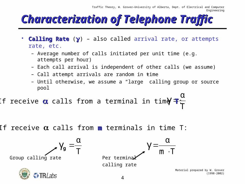
Characterization of Telephone Characterization of Telephone TrafficTraffic• Calling RateCalling Rate () – also called arrival rate, or attempts rate,
etc.– Average number of calls initiated per unit time (e.g. attempts per
hour)– Each call arrival is independent of other calls (we assume)– Call attempt arrivals are random in time– Until otherwise, we assume a “large” calling group or source pool
Tαγ If receive calls from a terminal in time TT:
If receive calls from mm terminals in time T:
Tαγ g
Group calling rateTm
αγ
Per terminalcalling rate
Material prepared by W. Grover (1998-2002)
5
Traffic Theory, W. Grover–University of Alberta, Dept. of Electrical and Computer Engineering
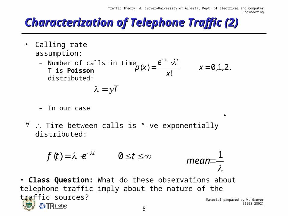
Characterization of Telephone Traffic Characterization of Telephone Traffic (2)(2)• Calling rate assumption:
– Number of calls in time T is Poisson distributed:
– In our case
...2 ,1 ,0!
)(
xx
exp
x
Time between calls is “-ve exponentially” distributed:
tetf t 0)( 1
mean
T
• Class Question: What do these observations about telephone traffic imply about the nature of the traffic sources?
Material prepared by W. Grover (1998-2002)
6
Traffic Theory, W. Grover–University of Alberta, Dept. of Electrical and Computer Engineering
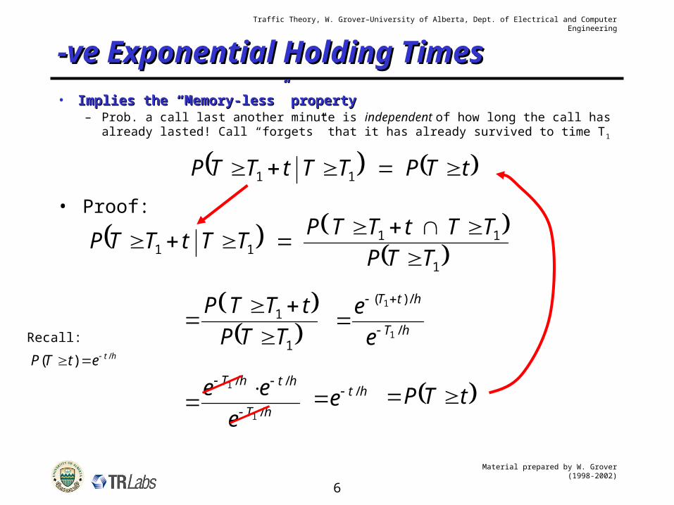
-ve Exponential Holding Times-ve Exponential Holding Times
• Implies the “Memory-less” propertyImplies the “Memory-less” property– Prob. a call last another minute is independent of how long the call has
already lasted! Call “forgets” that it has already survived to time T1
tTPTTtTTP 11
1
1111
TTP
TTtTTPTTtTTP
• Proof:
1
1
TTP
tTTP
hT
hthT
e
ee/
//
1
1
hte /
hT
htT
e
e/
/)(
1
1
tTP
htetTP /)(
Recall:
Material prepared by W. Grover (1998-2002)
7
Traffic Theory, W. Grover–University of Alberta, Dept. of Electrical and Computer Engineering
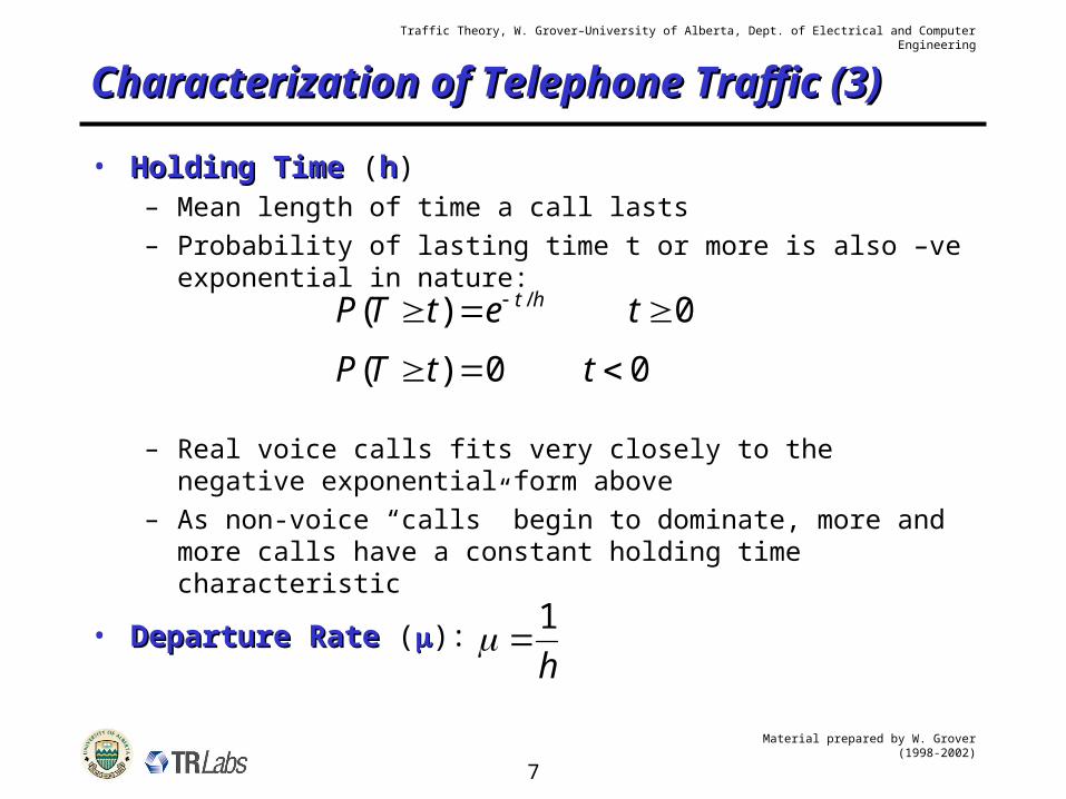
Characterization of Telephone Traffic Characterization of Telephone Traffic (3)(3)• Holding TimeHolding Time (hh)
– Mean length of time a call lasts– Probability of lasting time t or more is also –ve exponential
in nature:
– Real voice calls fits very closely to the negative exponential form above
– As non-voice “calls” begin to dominate, more and more calls have a constant holding time characteristic
• Departure RateDeparture Rate ():
0)( / tetTP ht
00)( ttTP
h
1
Material prepared by W. Grover (1998-2002)
8
Traffic Theory, W. Grover–University of Alberta, Dept. of Electrical and Computer Engineering
Some Real Holding Time DataSome Real Holding Time Data
Material prepared by W. Grover (1998-2002)
9
Traffic Theory, W. Grover–University of Alberta, Dept. of Electrical and Computer Engineering
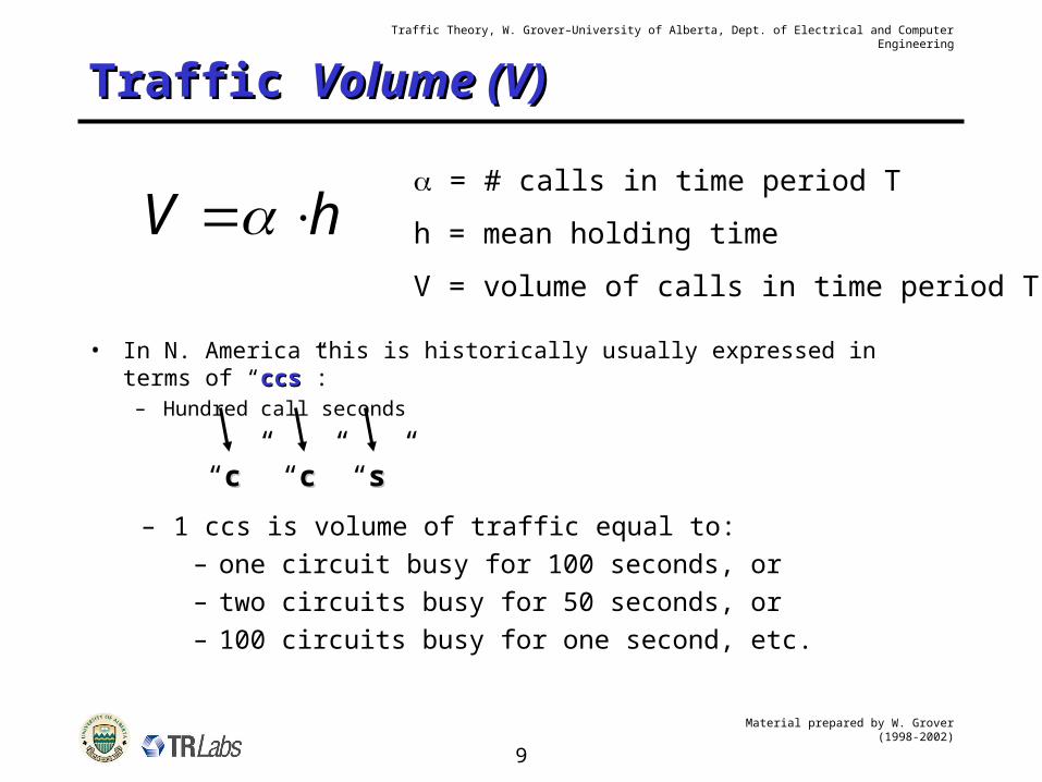
Traffic Traffic Volume (V)Volume (V)
hV = # calls in time period T
h = mean holding time
V = volume of calls in time period T
• In N. America this is historically usually expressed in terms of “ccsccs”:– Hundred call seconds
“cc” “cc” “ss”
– 1 ccs is volume of traffic equal to:– one circuit busy for 100 seconds, or– two circuits busy for 50 seconds, or– 100 circuits busy for one second, etc.
Material prepared by W. Grover (1998-2002)
10
Traffic Theory, W. Grover–University of Alberta, Dept. of Electrical and Computer Engineering
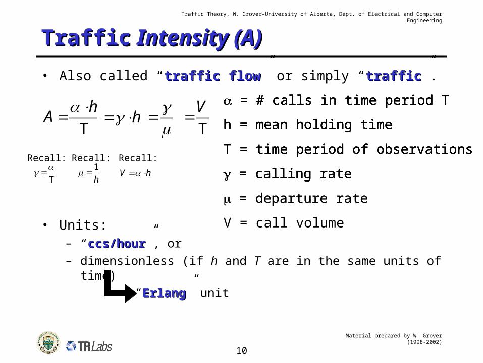
TrafficTraffic Intensity (A) Intensity (A)
• Also called “traffic flowtraffic flow” or simply “traffictraffic”.
= # calls in time period T
h = mean holding time
T = time period of observations
hA
T
• Units:– “ccs/hourccs/hour”, or– dimensionless (if h and T are in the same units of time)
“ErlangErlang” unit
h
= # calls in time period T
h = mean holding time
T = time period of observations
= calling rate
= # calls in time period T
h = mean holding time
T = time period of observations
= calling rate
= departure rate
T
Recall:
h
1
Recall:
V
T
V h
Recall:
= # calls in time period T
h = mean holding time
T = time period of observations
= calling rate
= departure rate
V = call volume
Material prepared by W. Grover (1998-2002)
11
Traffic Theory, W. Grover–University of Alberta, Dept. of Electrical and Computer Engineering
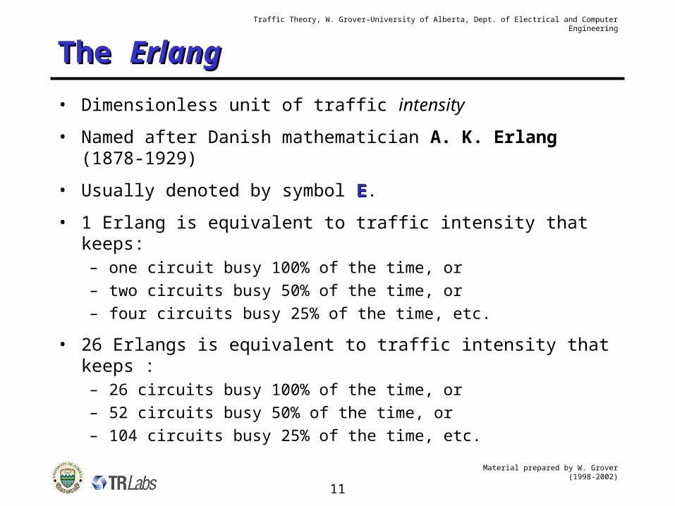
The The ErlangErlang
• Dimensionless unit of traffic intensity
• Named after Danish mathematician A. K. Erlang (1878-1929)
• Usually denoted by symbol EE.
• 1 Erlang is equivalent to traffic intensity that keeps:– one circuit busy 100% of the time, or– two circuits busy 50% of the time, or– four circuits busy 25% of the time, etc.
• 26 Erlangs is equivalent to traffic intensity that keeps :– 26 circuits busy 100% of the time, or– 52 circuits busy 50% of the time, or– 104 circuits busy 25% of the time, etc.
Material prepared by W. Grover (1998-2002)
13
Traffic Theory, W. Grover–University of Alberta, Dept. of Electrical and Computer Engineering
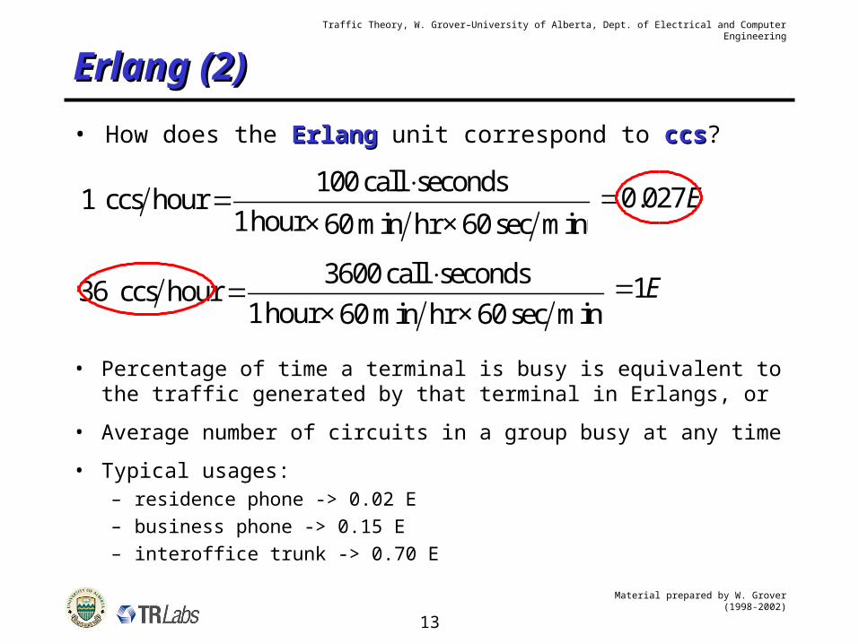
Erlang (2)Erlang (2)
• How does the ErlangErlang unit correspond to ccsccs?
• Percentage of time a terminal is busy is equivalent to the traffic generated by that terminal in Erlangs, or
• Average number of circuits in a group busy at any time
• Typical usages:– residence phone -> 0.02 E– business phone -> 0.15 E– interoffice trunk -> 0.70 E
0.027E
1E
100 call seconds1 ccs hour
1 hour × 60 min hr × 60 sec min
3600 call seconds36 ccs hour
1 hour × 60 min hr × 60 sec min
× 60 min hr × 60 sec min
× 60 min hr × 60 sec min
Material prepared by W. Grover (1998-2002)
14
Traffic Theory, W. Grover–University of Alberta, Dept. of Electrical and Computer Engineering
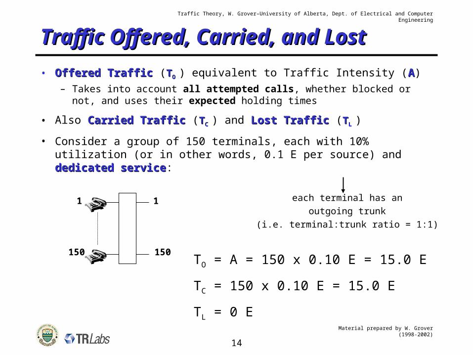
Traffic Offered, Carried, and LostTraffic Offered, Carried, and Lost
• Offered TrafficOffered Traffic (TTO O ) equivalent to Traffic Intensity (AA)– Takes into account all attempted calls, whether blocked or
not, and uses their expected holding times
• Also Carried Traffic Carried Traffic (TTC C ) and Lost TrafficLost Traffic (TTL L )
• Consider a group of 150 terminals, each with 10% utilization (or in other words, 0.1 E per source) and dedicated servicededicated service:
1
150
1
150
each terminal has anoutgoing trunk
(i.e. terminal:trunk ratio = 1:1)
TO = A = 150 x 0.10 E = 15.0 E
TC = 150 x 0.10 E = 15.0 E
TL = 0 E
Material prepared by W. Grover (1998-2002)
15
Traffic Theory, W. Grover–University of Alberta, Dept. of Electrical and Computer Engineering
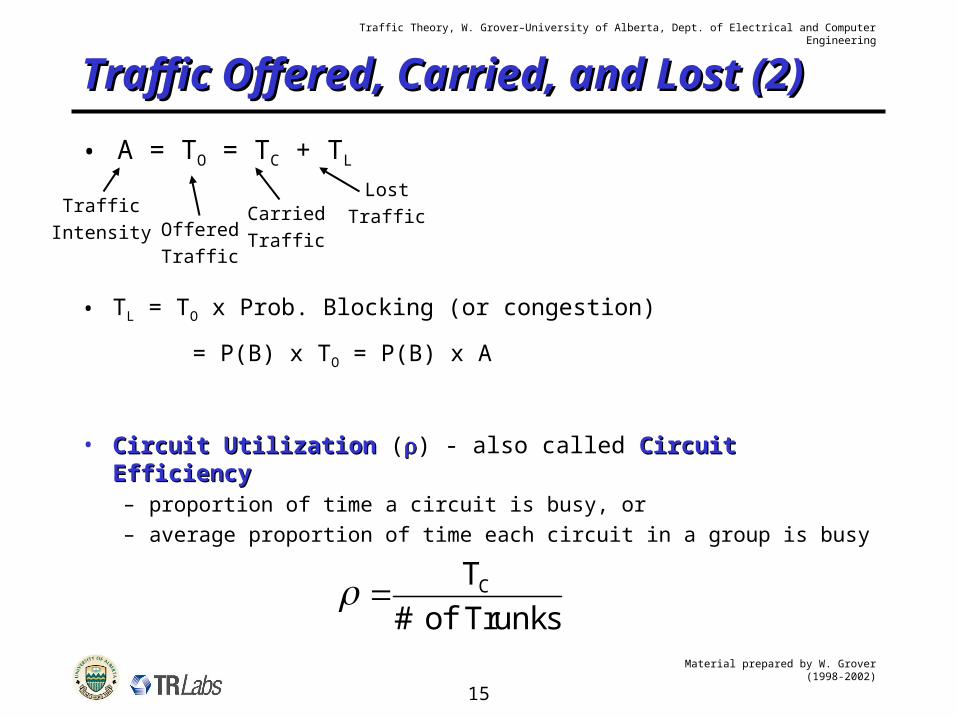
Traffic Offered, Carried, and Lost Traffic Offered, Carried, and Lost (2)(2)• A = TO = TC + TL
TrafficIntensity Offered
Traffic
CarriedTraffic
LostTraffic
• TL = TO x Prob. Blocking (or congestion)
= P(B) x TO = P(B) x A
• Circuit UtilizationCircuit Utilization () - also called Circuit EfficiencyCircuit Efficiency– proportion of time a circuit is busy, or– average proportion of time each circuit in a group is busy
CT # of Trunks
Material prepared by W. Grover (1998-2002)
16
Traffic Theory, W. Grover–University of Alberta, Dept. of Electrical and Computer Engineering
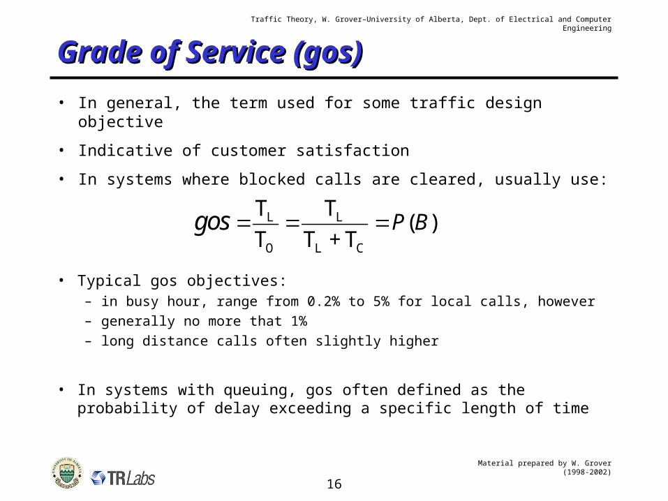
Grade of Service (gos)Grade of Service (gos)
• In general, the term used for some traffic design objective
• Indicative of customer satisfaction
• In systems where blocked calls are cleared, usually use:
L L
O L C
T T( )
T T + TP Bgos
• Typical gos objectives:– in busy hour, range from 0.2% to 5% for local calls, however– generally no more that 1%– long distance calls often slightly higher
• In systems with queuing, gos often defined as the probability of delay exceeding a specific length of time
Material prepared by W. Grover (1998-2002)
17
Traffic Theory, W. Grover–University of Alberta, Dept. of Electrical and Computer Engineering
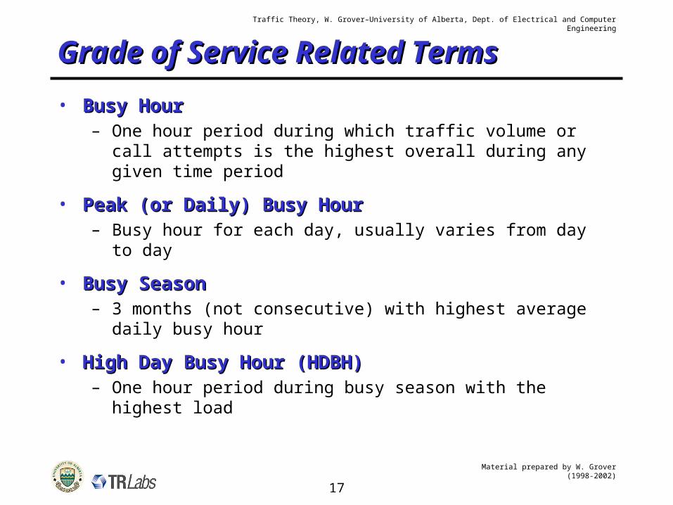
Grade of Service Related TermsGrade of Service Related Terms
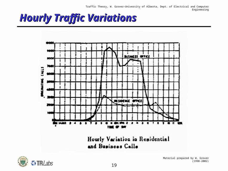
• Busy HourBusy Hour– One hour period during which traffic volume or call
attempts is the highest overall during any given time period
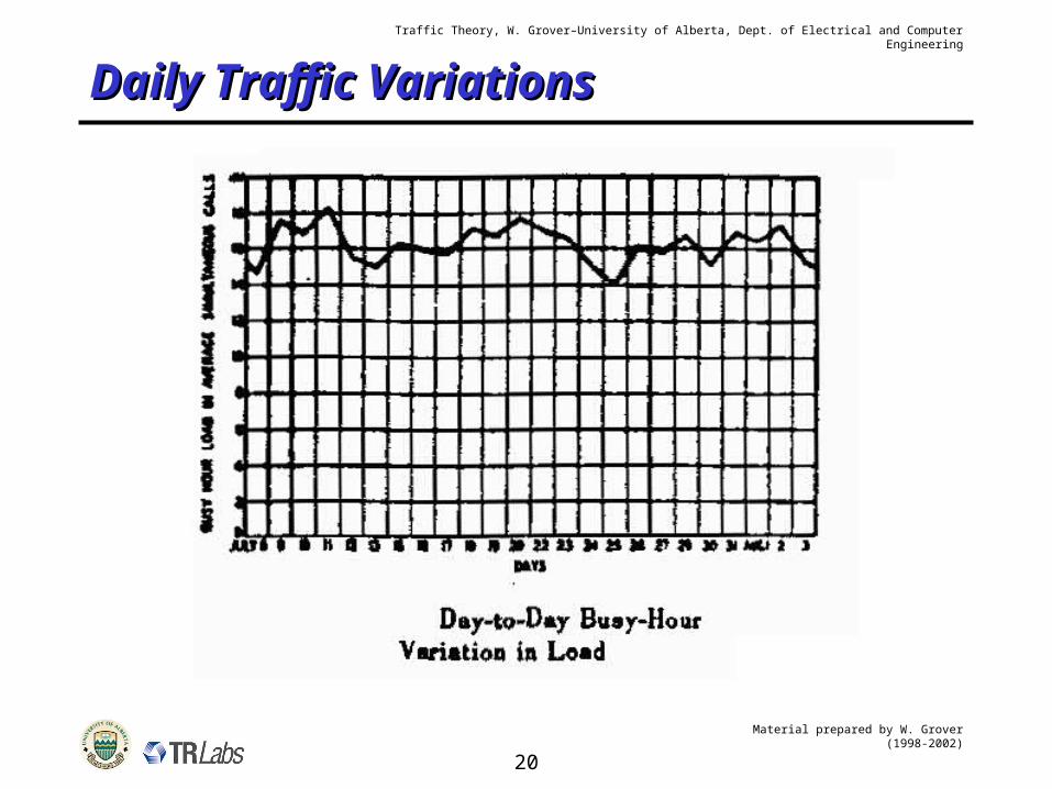
• Peak (or Daily) Busy HourPeak (or Daily) Busy Hour– Busy hour for each day, usually varies from day to day
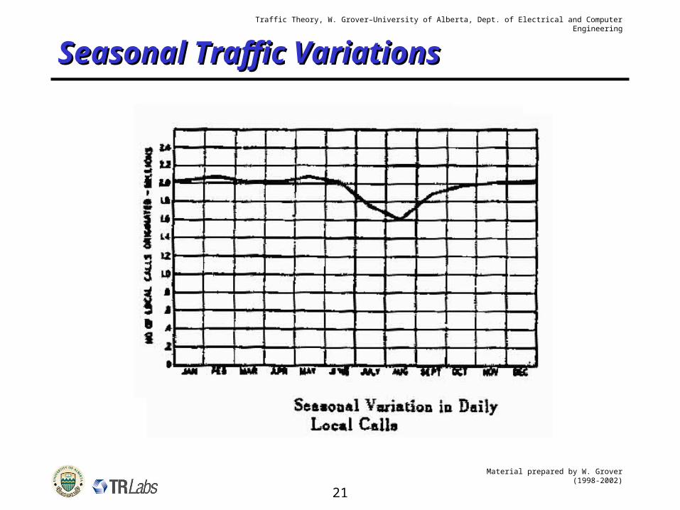
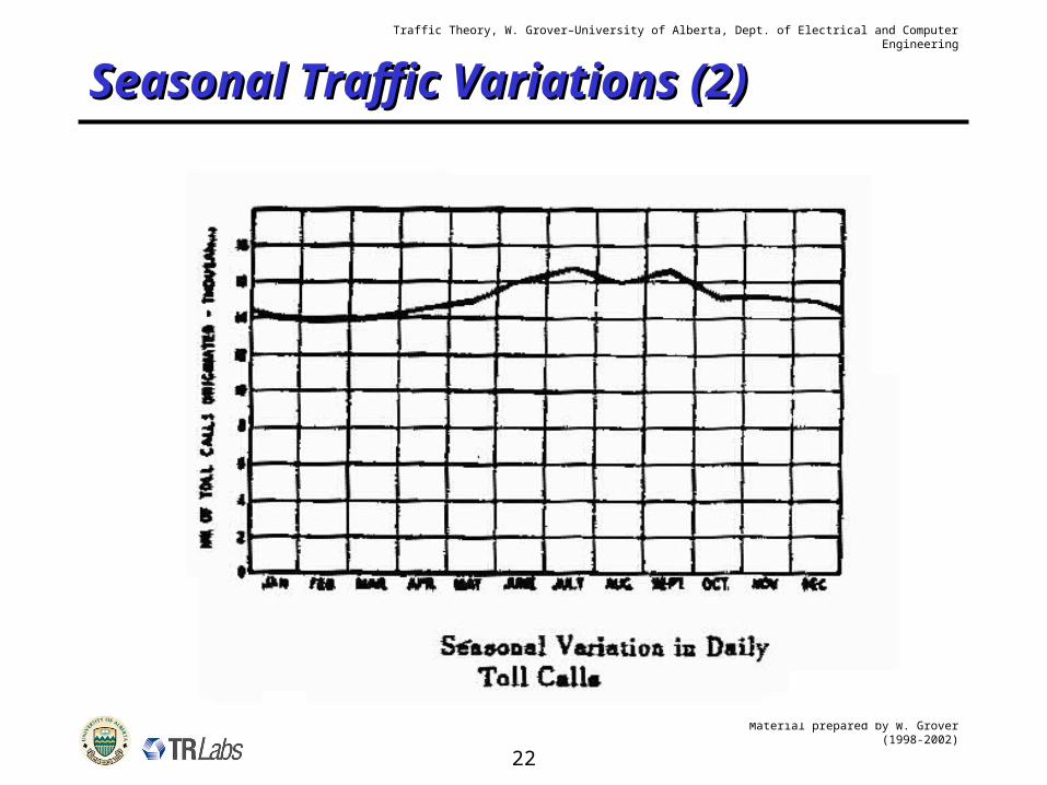
• Busy SeasonBusy Season– 3 months (not consecutive) with highest average daily
busy hour
• High Day Busy Hour (HDBH)High Day Busy Hour (HDBH)– One hour period during busy season with the highest load
Material prepared by W. Grover (1998-2002)
18
Traffic Theory, W. Grover–University of Alberta, Dept. of Electrical and Computer Engineering
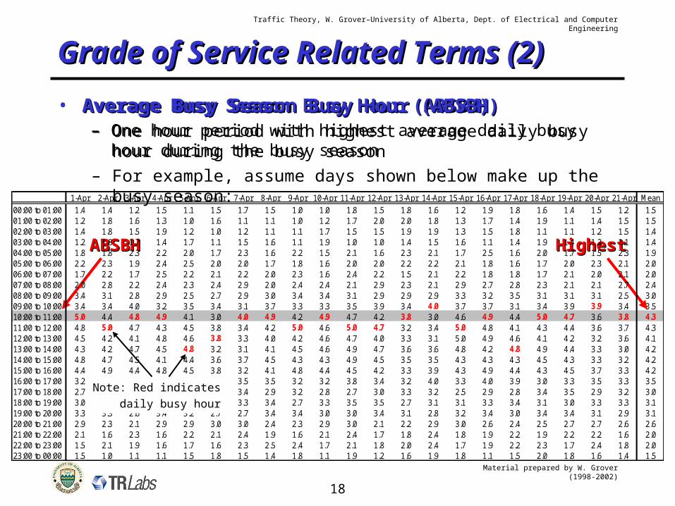
Grade of Service Related Terms Grade of Service Related Terms (2)(2)
HighestHighestABSBHABSBH
• Average Busy Season Busy Hour (ABSBH)Average Busy Season Busy Hour (ABSBH)– One hour period with highest average daily busy hour
during the busy season
• Average Busy Season Busy Hour (ABSBH)Average Busy Season Busy Hour (ABSBH)– One hour period with highest average daily busy hour
during the busy season– For example, assume days shown below make up the busy
Traffic Theory, W. Grover–University of Alberta, Dept. of Electrical and Computer Engineering
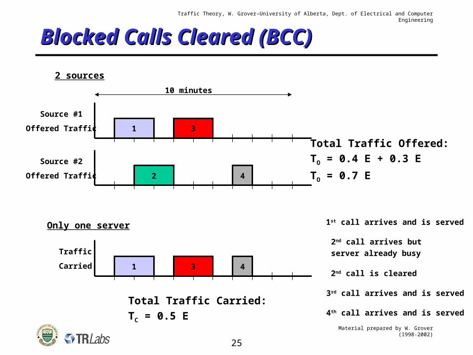
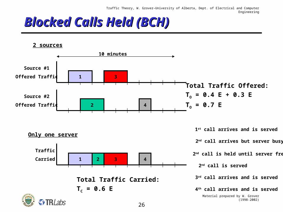
Source #1
Offered Traffic
Source #2
Offered Traffic
1
2
3
4
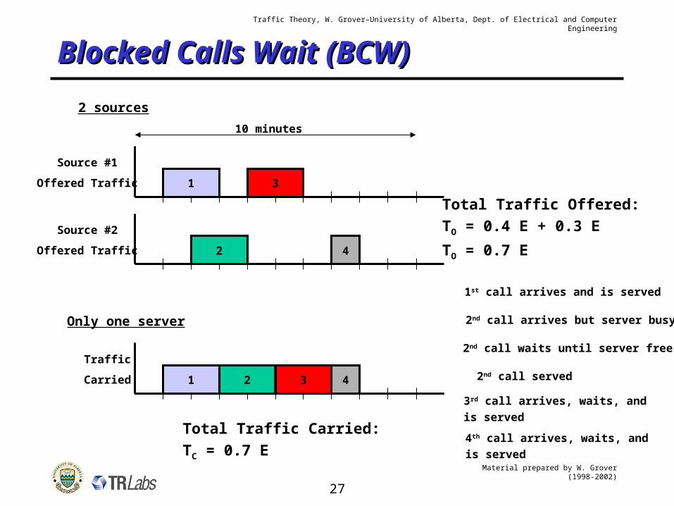
10 minutes
Total Traffic Offered:TO = 0.4 E + 0.3 E
TO = 0.7 E
2 sources
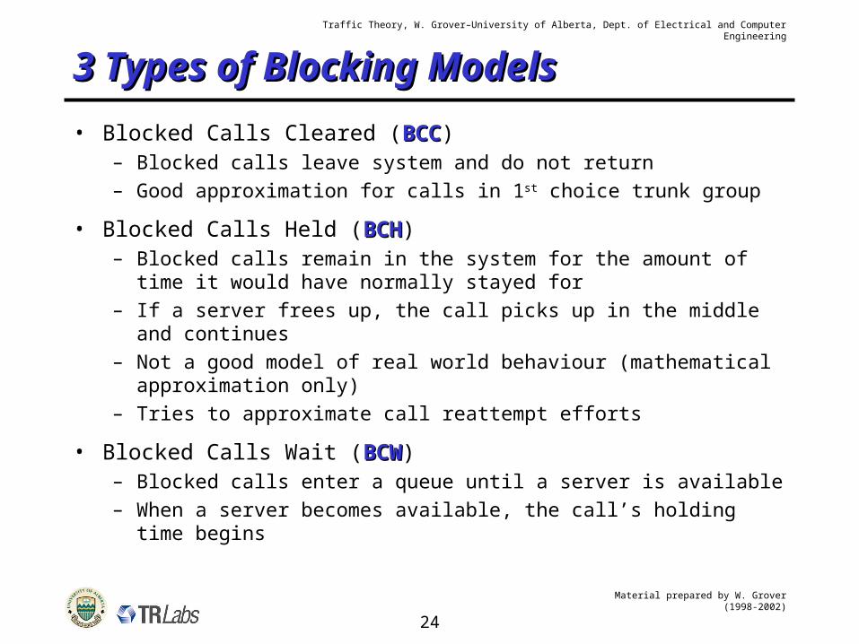
Blocked Calls Held (BCH)Blocked Calls Held (BCH)
Traffic
Carried 1 21 2 3 4
Only one server1st call arrives and is served
2nd call arrives but server busy
2nd call is served
3rd call arrives and is served
4th call arrives and is served
Total Traffic Carried:TC = 0.6 E
2nd call is held until server free
Material prepared by W. Grover (1998-2002)
27
Traffic Theory, W. Grover–University of Alberta, Dept. of Electrical and Computer Engineering
Source #1
Offered Traffic
Source #2
Offered Traffic
1
2
3
4
10 minutes
Total Traffic Offered:TO = 0.4 E + 0.3 E
TO = 0.7 E
2 sources
Blocked Calls Wait (BCW)Blocked Calls Wait (BCW)
Only one server
Traffic
Carried
1st call arrives and is served
1
2nd call arrives but server busy
2
2nd call waits until server free
2nd call served1 2
3rd call arrives, waits, and is served
3
4th call arrives, waits, andis served
4
Total Traffic Carried:TC = 0.7 E
Material prepared by W. Grover (1998-2002)
28
Traffic Theory, W. Grover–University of Alberta, Dept. of Electrical and Computer Engineering
Blocking ProbabilitiesBlocking Probabilities
• System must be in a Steady StateSteady State– Also called state of statistical equilibrium– Arrival RateArrival Rate of new calls equals Departure RateDeparture Rate of
disconnecting calls– Why?
• If calls arrive faster that they depart?• If calls depart faster than they arrive?
Material prepared by W. Grover (1998-2002)
29
Traffic Theory, W. Grover–University of Alberta, Dept. of Electrical and Computer Engineering
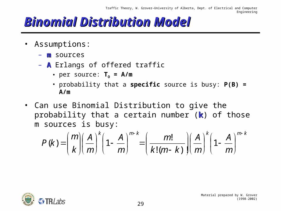
Binomial Distribution ModelBinomial Distribution Model
• Assumptions:– mm sources– AA Erlangs of offered traffic
• per source: TO = A/m
• probability that a specific source is busy: P(B) = A/m
• Can use Binomial Distribution to give the probability that a certain number (kk) of those m sources is busy:
kmk
m
A
m
A
k
mkP
1)(
kmk
m
A
m
A
kmk
m
1)!(!
!
Material prepared by W. Grover (1998-2002)
30
Traffic Theory, W. Grover–University of Alberta, Dept. of Electrical and Computer Engineering
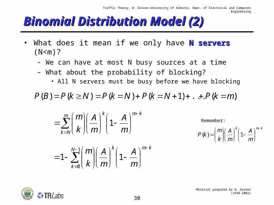
Binomial Distribution Model (2)Binomial Distribution Model (2)
• What does it mean if we only have N serversN servers (N<m)?– We can have at most N busy sources at a time– What about the probability of blocking?
• All N servers must be busy before we have blocking
)()( NkPBP )(...)1()( mkPNkPNkP
kmk
m
A
m
A
k
mkP
1)(
m
Nk
kmk
m
A
m
A
k
m1
1
0
11N
k
kmk
m
A
m
A
k
m
Remember:
Material prepared by W. Grover (1998-2002)
31
Traffic Theory, W. Grover–University of Alberta, Dept. of Electrical and Computer Engineering
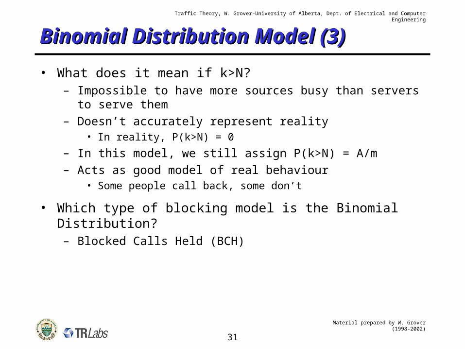
Binomial Distribution Model (3)Binomial Distribution Model (3)
• What does it mean if k>N?– Impossible to have more sources busy than servers to
serve them– Doesn’t accurately represent reality
• In reality, P(k>N) = 0
– In this model, we still assign P(k>N) = A/m – Acts as good model of real behaviour
• Some people call back, some don’t
• Which type of blocking model is the Binomial Distribution?– Blocked Calls Held (BCH)
Material prepared by W. Grover (1998-2002)
32
Traffic Theory, W. Grover–University of Alberta, Dept. of Electrical and Computer Engineering
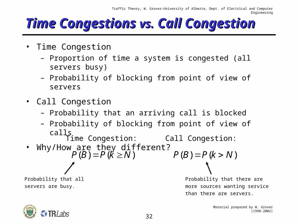
Time Congestions Time Congestions vs.vs. Call Call CongestionCongestion• Time Congestion
– Proportion of time a system is congested (all servers busy)– Probability of blocking from point of view of servers
• Call Congestion– Probability that an arriving call is blocked– Probability of blocking from point of view of calls
• Why/How are they different?
Time Congestion:
)()( NkPBP
Probability that allservers are busy.
Call Congestion:
)()( NkPBP
Probability that there aremore sources wanting servicethan there are servers.
Material prepared by W. Grover (1998-2002)
33
Traffic Theory, W. Grover–University of Alberta, Dept. of Electrical and Computer Engineering
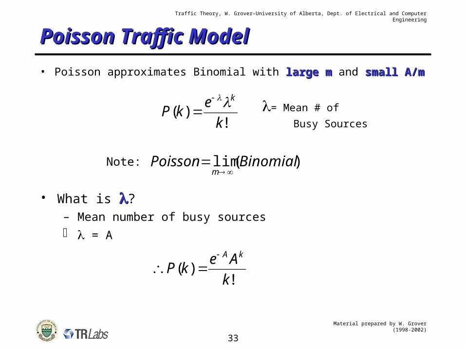
Poisson Traffic ModelPoisson Traffic Model
• Poisson approximates Binomial with large mlarge m and small A/msmall A/m
!)(
k
ekP
k = Mean # of
Busy Sources
Note: )(lim BinomialPoissonm
• What is ?– Mean number of busy sources = A
!)(
k
AekP
kA
Material prepared by W. Grover (1998-2002)
34
Traffic Theory, W. Grover–University of Alberta, Dept. of Electrical and Computer Engineering
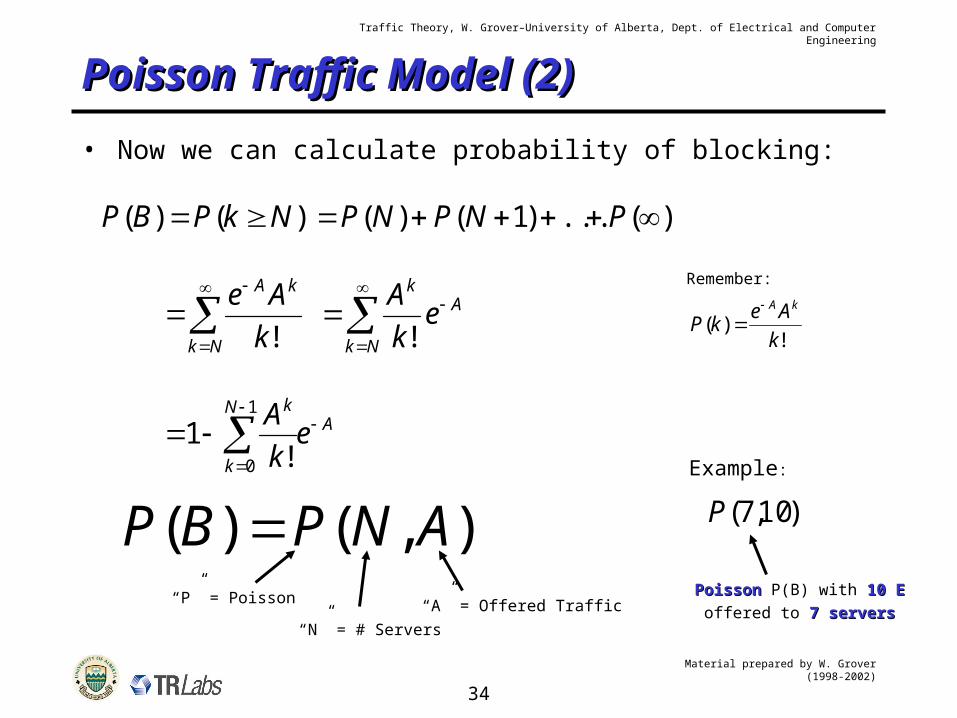
Poisson Traffic Model (2)Poisson Traffic Model (2)
• Now we can calculate probability of blocking:
)()( NkPBP )(...)1()( PNPNP
Remember:
!)(
k
AekP
kA
Nk
kA
k
Ae
!
Nk
Ak
ek
A
!
AN
k
k
ek
A
1
0 !1
),()( ANPBP “P” = Poisson
“N” = # Servers
“A” = Offered Traffic
Example:
)10,7(P
PoissonPoisson P(B) with 10 E10 Eoffered to 7 servers7 servers
Material prepared by W. Grover (1998-2002)
35
Traffic Theory, W. Grover–University of Alberta, Dept. of Electrical and Computer Engineering
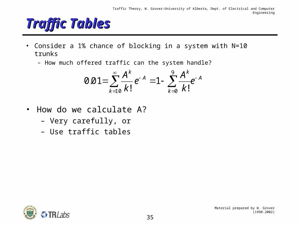
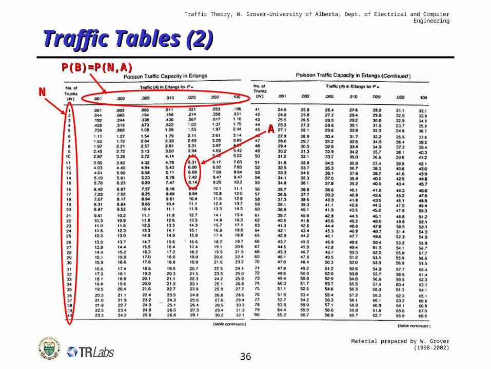
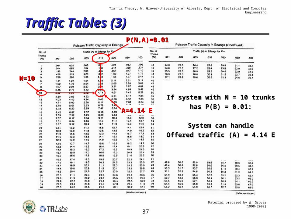
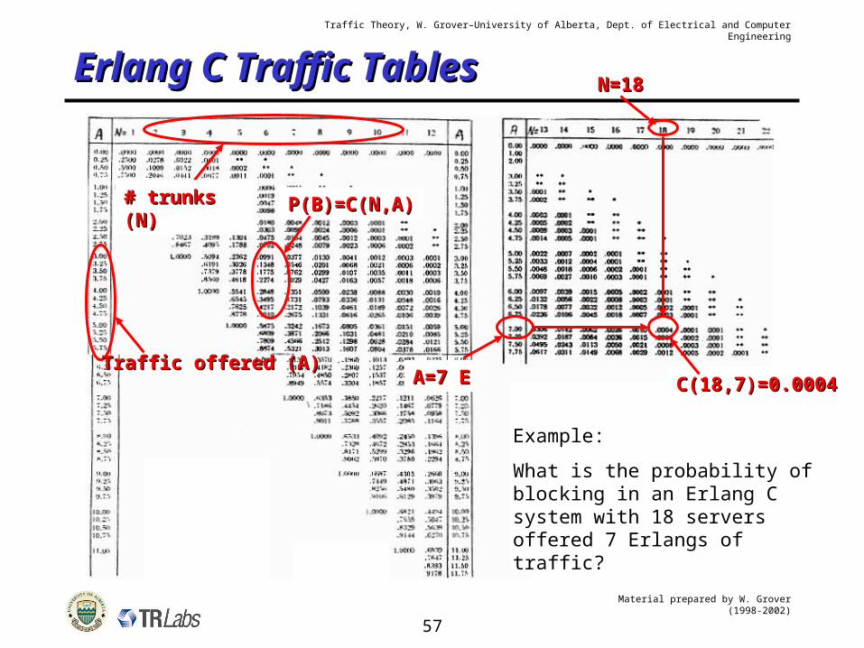
Traffic TablesTraffic Tables
• Consider a 1% chance of blocking in a system with N=10 trunks– How much offered traffic can the system handle?
A
k
k
k
Ak
ek
Ae
k
A
9
010 !1
!01.0
• How do we calculate A?– Very carefully, or– Use traffic tables
Material prepared by W. Grover (1998-2002)
36
Traffic Theory, W. Grover–University of Alberta, Dept. of Electrical and Computer Engineering
Traffic Theory, W. Grover–University of Alberta, Dept. of Electrical and Computer Engineering
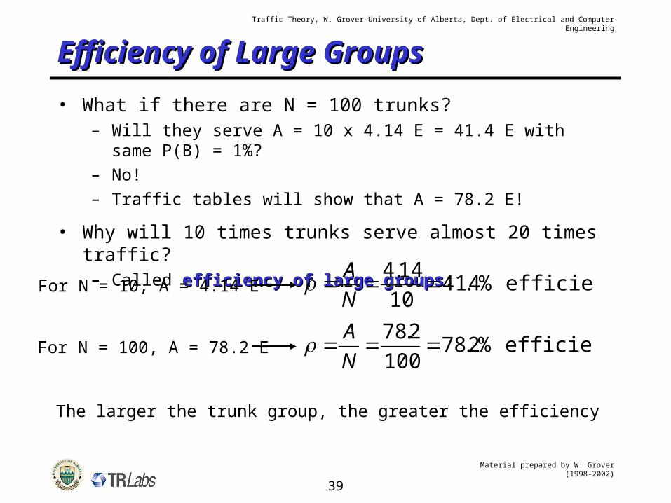
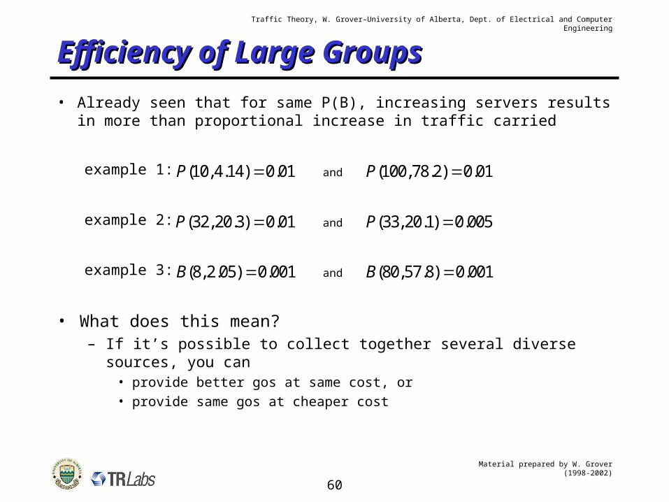
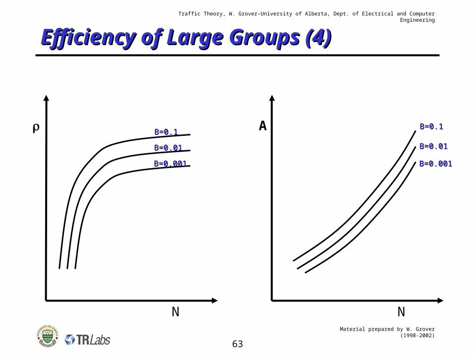
Efficiency of Large GroupsEfficiency of Large Groups
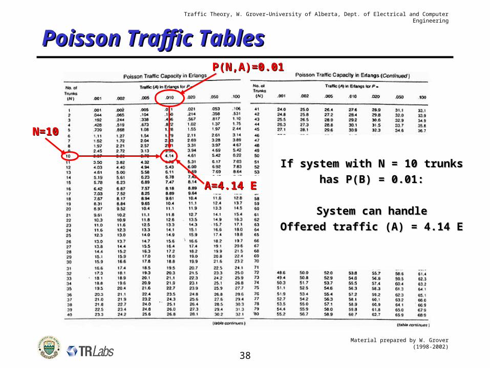
• What if there are N = 100 trunks?– Will they serve A = 10 x 4.14 E = 41.4 E with same P(B) =
1%?– No!– Traffic tables will show that A = 78.2 E!
• Why will 10 times trunks serve almost 20 times traffic?– Called efficiency of large groupsefficiency of large groups:
For N = 10, A = 4.14 E efficiency %4.4110
14.4
N
A
For N = 100, A = 78.2 E efficiency %2.78100
2.78
N
A
The larger the trunk group, the greater the efficiency
Material prepared by W. Grover (1998-2002)
40
Traffic Theory, W. Grover–University of Alberta, Dept. of Electrical and Computer Engineering
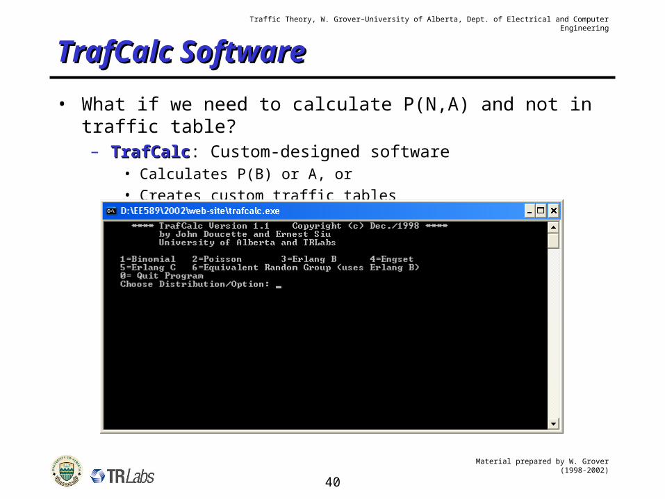
TrafCalc SoftwareTrafCalc Software
• What if we need to calculate P(N,A) and not in traffic table?– TrafCalcTrafCalc: Custom-designed software
• Calculates P(B) or A, or• Creates custom traffic tables
Material prepared by W. Grover (1998-2002)
41
Traffic Theory, W. Grover–University of Alberta, Dept. of Electrical and Computer Engineering
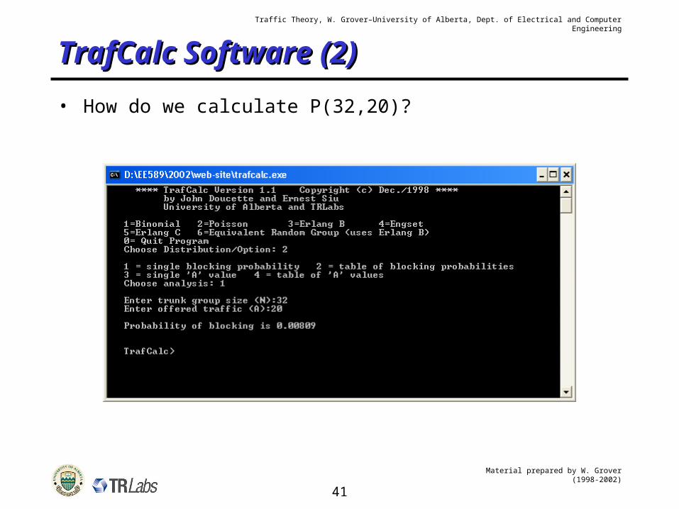
TrafCalc Software (2)TrafCalc Software (2)
• How do we calculate P(32,20)?
Material prepared by W. Grover (1998-2002)
42
Traffic Theory, W. Grover–University of Alberta, Dept. of Electrical and Computer Engineering
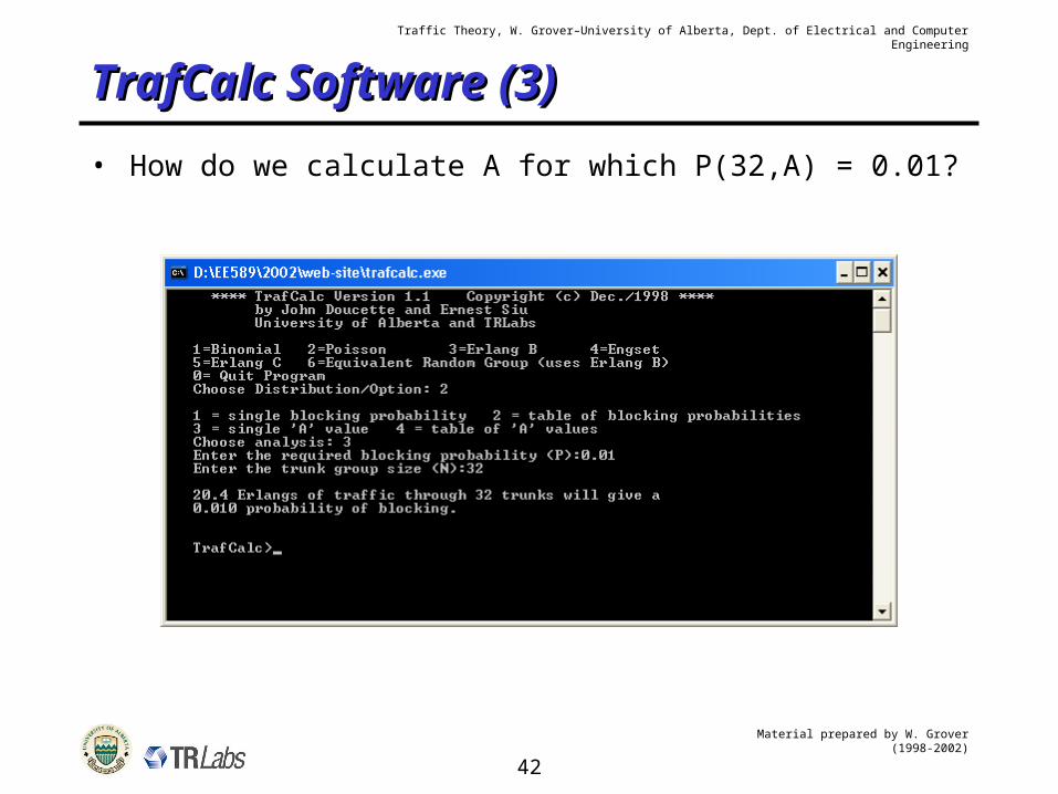
TrafCalc Software (3)TrafCalc Software (3)
• How do we calculate A for which P(32,A) = 0.01?
Material prepared by W. Grover (1998-2002)
43
Traffic Theory, W. Grover–University of Alberta, Dept. of Electrical and Computer Engineering
Erlang B ModelErlang B Model
• More sophisticated model than Binomial or Poisson
• Blocked Calls Cleared (BCC)
• Good for calls that can reroute to alternate route if blocked
• No approximation for reattempts if alternate route blocked too
• Derived using birth-death processbirth-death process– See selected pages from Leonard Kleinrock, Queueing
Systems Volume 1: Theory, John Wiley & Sons, 1975
Material prepared by W. Grover (1998-2002)
44
Traffic Theory, W. Grover–University of Alberta, Dept. of Electrical and Computer Engineering
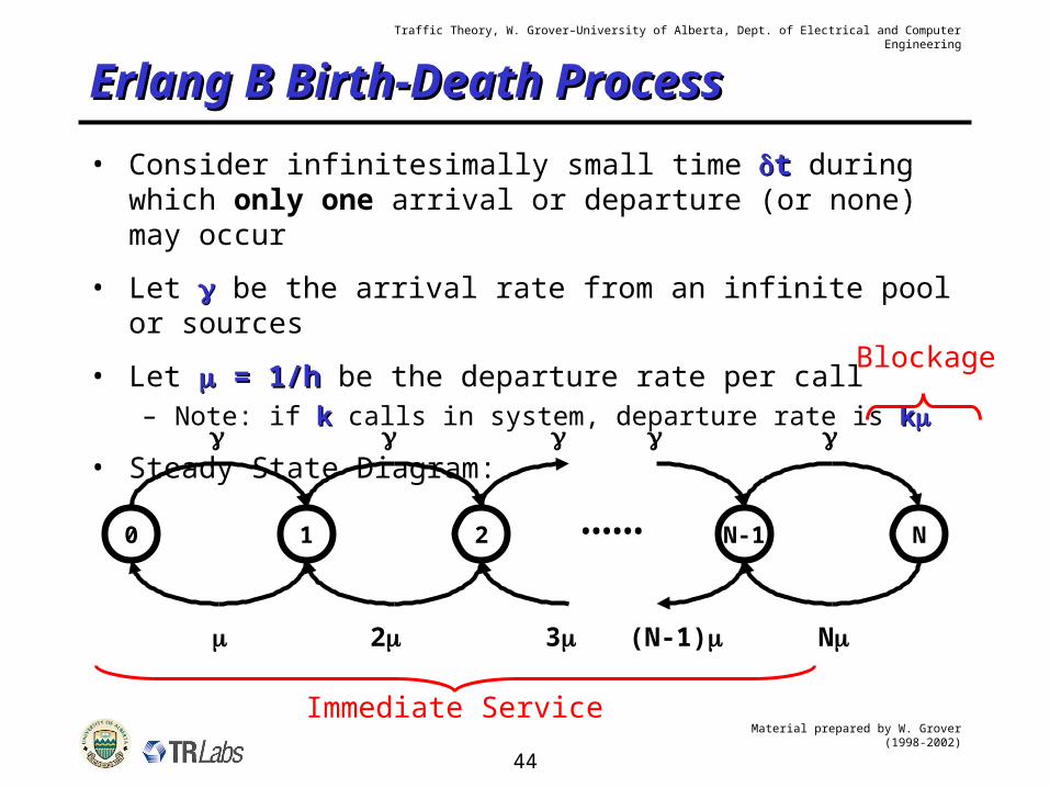
Erlang B Birth-Death ProcessErlang B Birth-Death Process
• Consider infinitesimally small time tt during which only one arrival or departure (or none) may occur
• Let be the arrival rate from an infinite pool or sources
• Let = 1/h = 1/h be the departure rate per call– Note: if kk calls in system, departure rate is kk
• Steady State Diagram:
0 1 2 N-1 N……
2
N(N-1)3
Immediate Service
Blockage
Material prepared by W. Grover (1998-2002)
45
Traffic Theory, W. Grover–University of Alberta, Dept. of Electrical and Computer Engineering
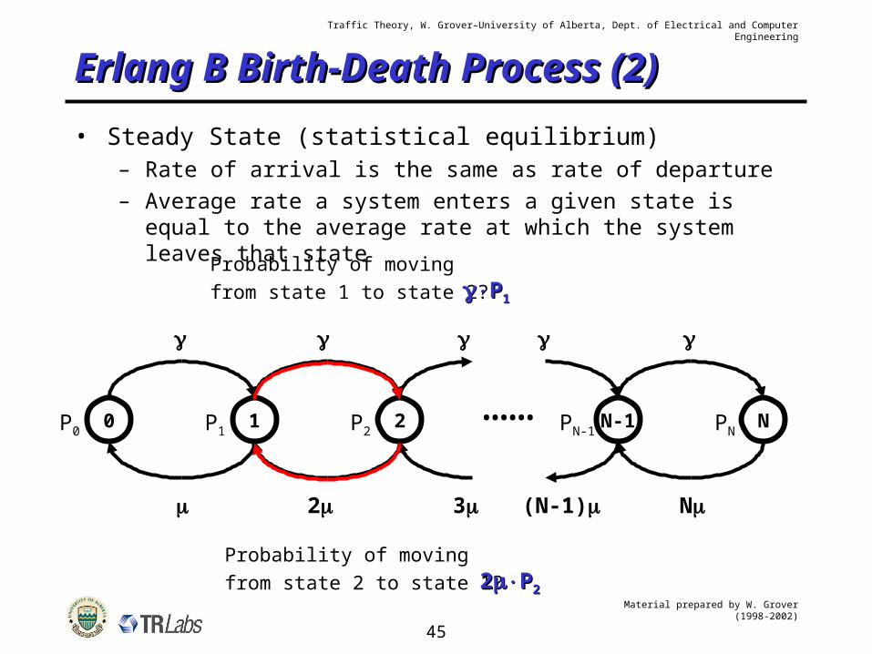
Erlang B Birth-Death Process (2)Erlang B Birth-Death Process (2)
• Steady State (statistical equilibrium)– Rate of arrival is the same as rate of departure– Average rate a system enters a given state is equal to the
average rate at which the system leaves that state
0 1 2 N-1 N……
2
N(N-1)3
P0 P1 P2 PN-1 PN
Probability of movingfrom state 1 to state 2?PP11
Probability of movingfrom state 2 to state 1?22PP22
Material prepared by W. Grover (1998-2002)
46
Traffic Theory, W. Grover–University of Alberta, Dept. of Electrical and Computer Engineering
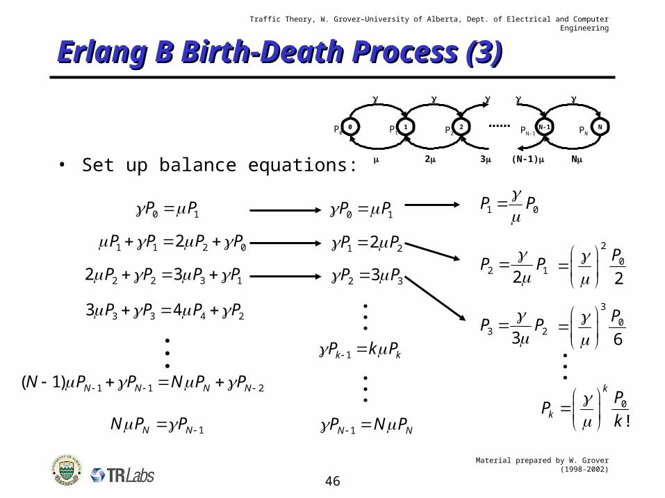
Erlang B Birth-Death Process (3)Erlang B Birth-Death Process (3)
• Set up balance equations:
0 1 2 N-1 N……
2
N(N-1)3
P0 P1 P2 PN-1 PN
0 1P P
1 1 2 02P P P P
2 2 3 12 3P P P P
3 3 4 23 4P P P P
1 1 2( 1) N N N NN P P N P P
1N NN P P
0 1P P
1 22P P
2 33P P
1k kP k P
1N NP N P
1 0P P
2 12P P
2
0
2
P
3 23P P
3
0
6
P
0
!
k
k
PP
k
Material prepared by W. Grover (1998-2002)
47
Traffic Theory, W. Grover–University of Alberta, Dept. of Electrical and Computer Engineering
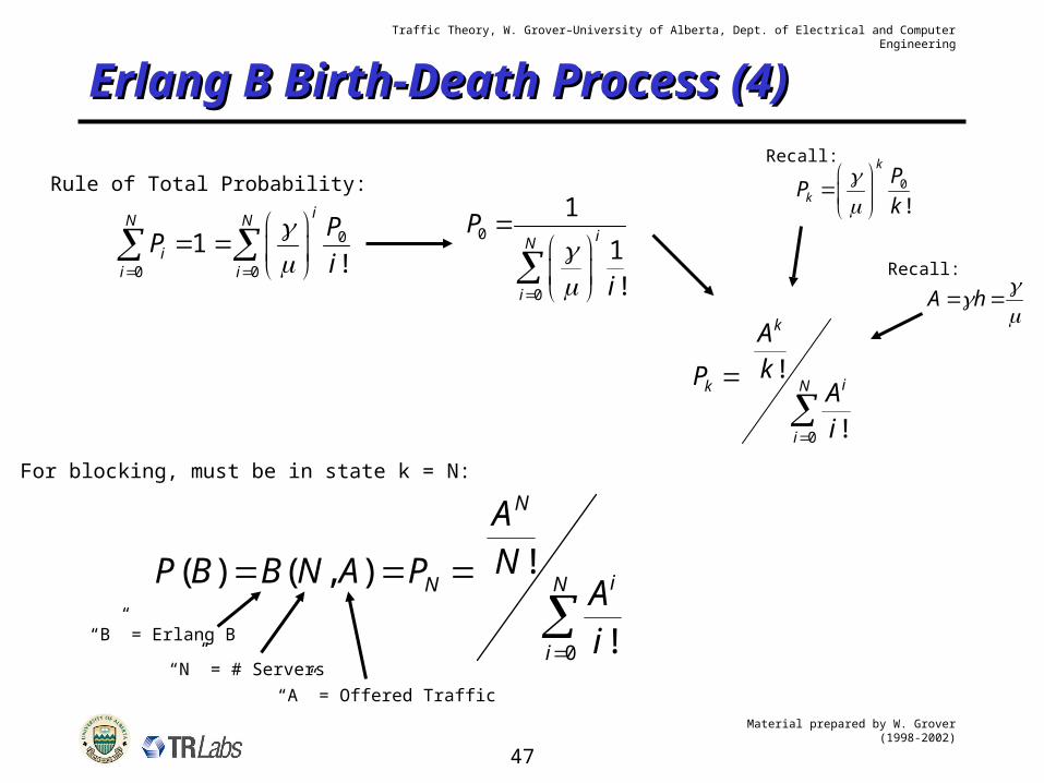
Erlang B Birth-Death Process (4)Erlang B Birth-Death Process (4)
Rule of Total Probability:
0
1N
ii
P
0
0 !
iN
i
P
i
0
0
1
1!
iN
i
P
i
0
!
k
k
PP
k
Recall:
0
1!
1!
k
k iN
i
kP
i
A h
Recall:
0
!
!
k
iNk
i
AkP
Ai
For blocking, must be in state k = N:
( ) ( , ) NP B B N A P
“B” = Erlang B
“N” = # Servers
“A” = Offered Traffic
0
!
!
N
iN
i
AN
Ai
Material prepared by W. Grover (1998-2002)
48
Traffic Theory, W. Grover–University of Alberta, Dept. of Electrical and Computer Engineering
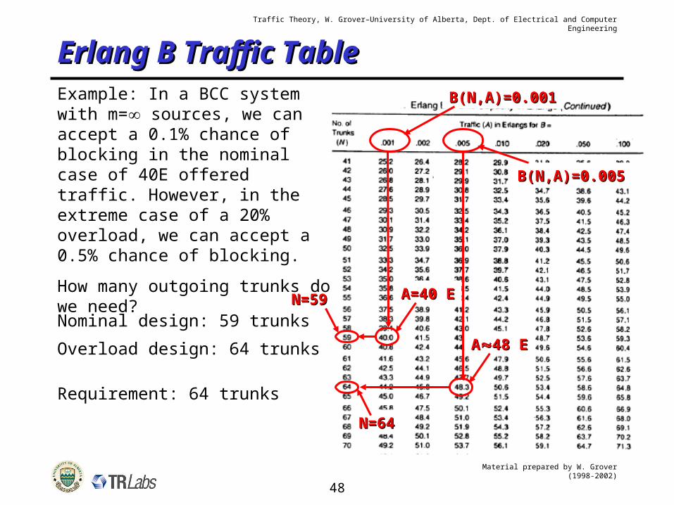
Erlang B Traffic TableErlang B Traffic Table
Example: In a BCC system with m= sources, we can accept a 0.1% chance of blocking in the nominal case of 40E offered traffic. However, in the extreme case of a 20% overload, we can accept a 0.5% chance of blocking.
How many outgoing trunks do we need?
B(N,A)=0.001B(N,A)=0.001
A=40 EA=40 EN=59N=59
Nominal design: 59 trunks
B(N,A)=0.005B(N,A)=0.005
AA48 E48 E
N=64N=64
Overload design: 64 trunks
Requirement: 64 trunks
Material prepared by W. Grover (1998-2002)
49
Traffic Theory, W. Grover–University of Alberta, Dept. of Electrical and Computer Engineering
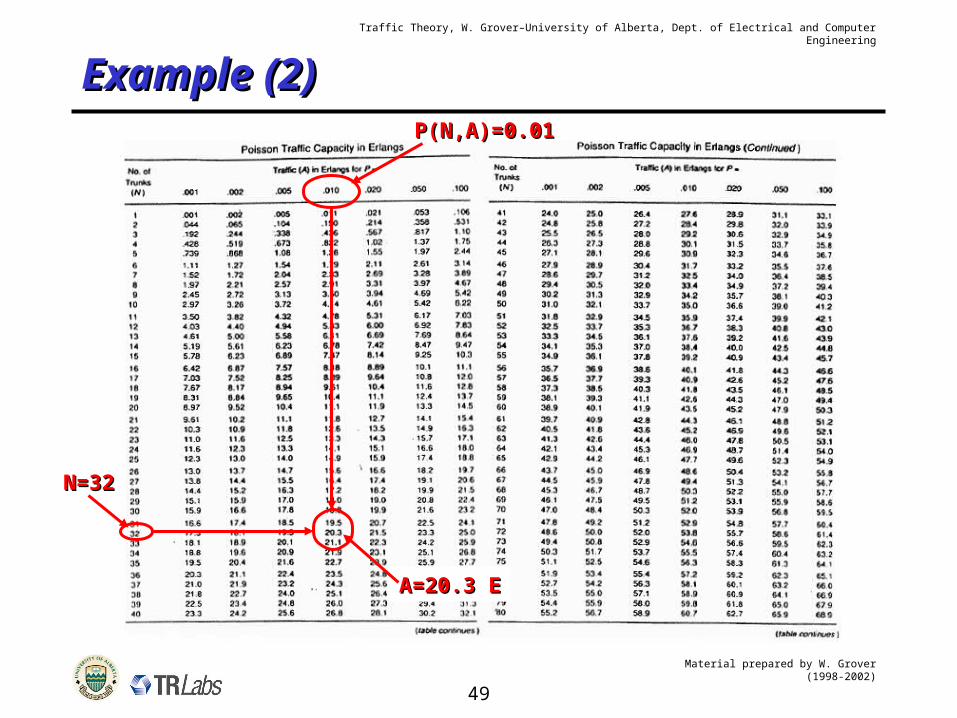
Example (2)Example (2)P(N,A)=0.01P(N,A)=0.01
N=32N=32
A=20.3 EA=20.3 E
Material prepared by W. Grover (1998-2002)
50
Traffic Theory, W. Grover–University of Alberta, Dept. of Electrical and Computer Engineering
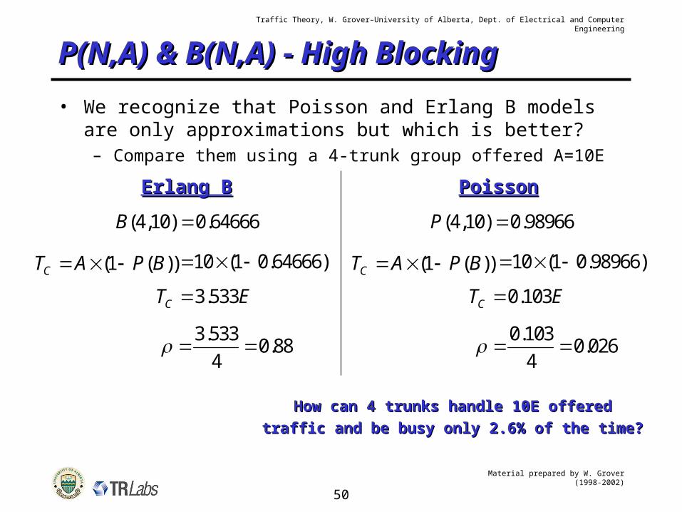
P(N,A) & B(N,A) - High BlockingP(N,A) & B(N,A) - High Blocking
• We recognize that Poisson and Erlang B models are only approximations but which is better?– Compare them using a 4-trunk group offered A=10E
Erlang BErlang B
(4,10) 0.64666B
(1 ( ))CT A P B 10 (1 0.64666)
3.533CT E
3.5330.88
4
PoissonPoisson
(4,10) 0.98966P
(1 ( ))CT A P B 10 (1 0.98966)
0.103CT E
0.1030.026
4
How can 4 trunks handle 10E offeredHow can 4 trunks handle 10E offered
traffic and be busy only 2.6% of the time?traffic and be busy only 2.6% of the time?
Material prepared by W. Grover (1998-2002)
51
Traffic Theory, W. Grover–University of Alberta, Dept. of Electrical and Computer Engineering
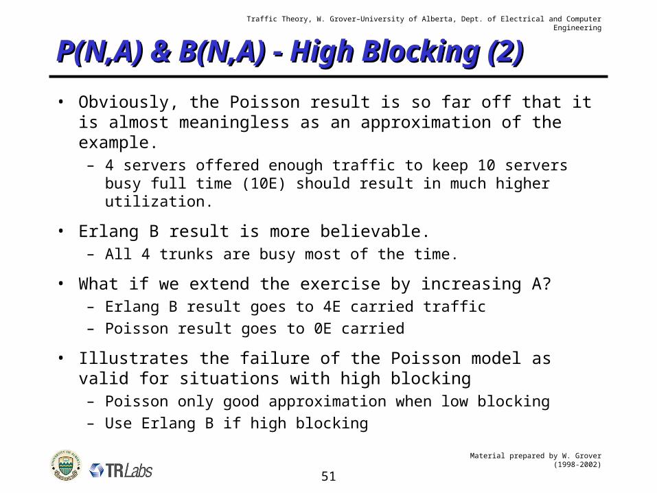
P(N,A) & B(N,A) - High Blocking P(N,A) & B(N,A) - High Blocking (2)(2)• Obviously, the Poisson result is so far off that it is almost
meaningless as an approximation of the example.– 4 servers offered enough traffic to keep 10 servers busy
full time (10E) should result in much higher utilization.
• Erlang B result is more believable.– All 4 trunks are busy most of the time.
• What if we extend the exercise by increasing A?– Erlang B result goes to 4E carried traffic– Poisson result goes to 0E carried
• Illustrates the failure of the Poisson model as valid for situations with high blocking– Poisson only good approximation when low blocking– Use Erlang B if high blocking
Material prepared by W. Grover (1998-2002)
52
Traffic Theory, W. Grover–University of Alberta, Dept. of Electrical and Computer Engineering
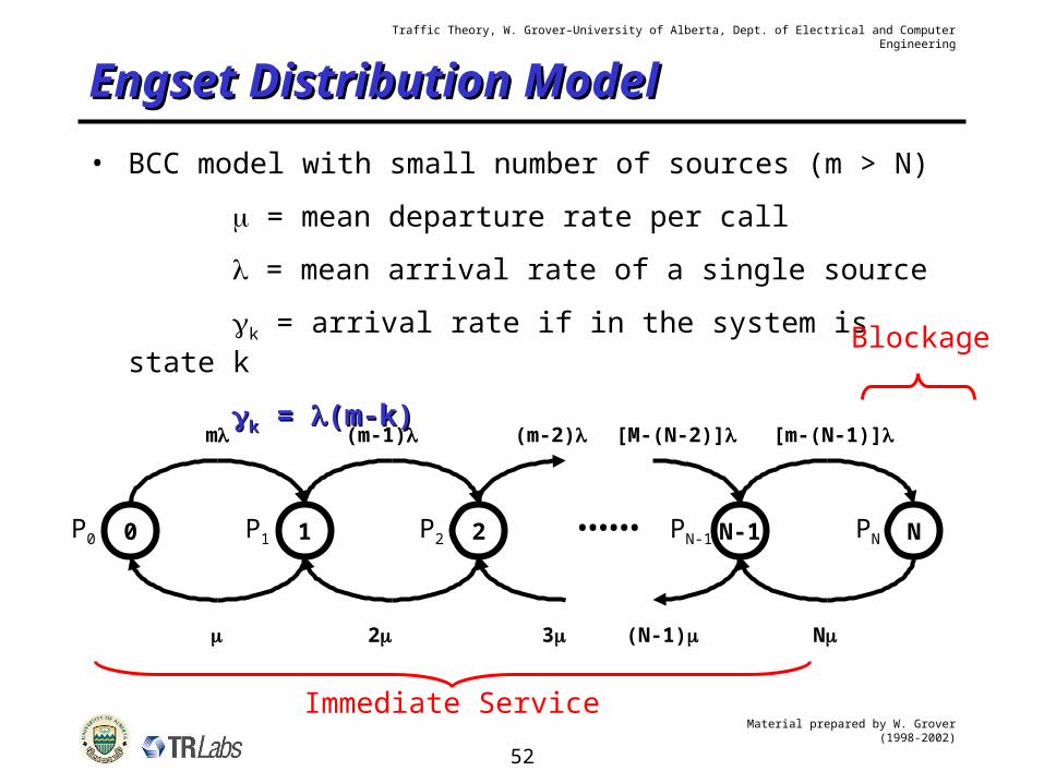
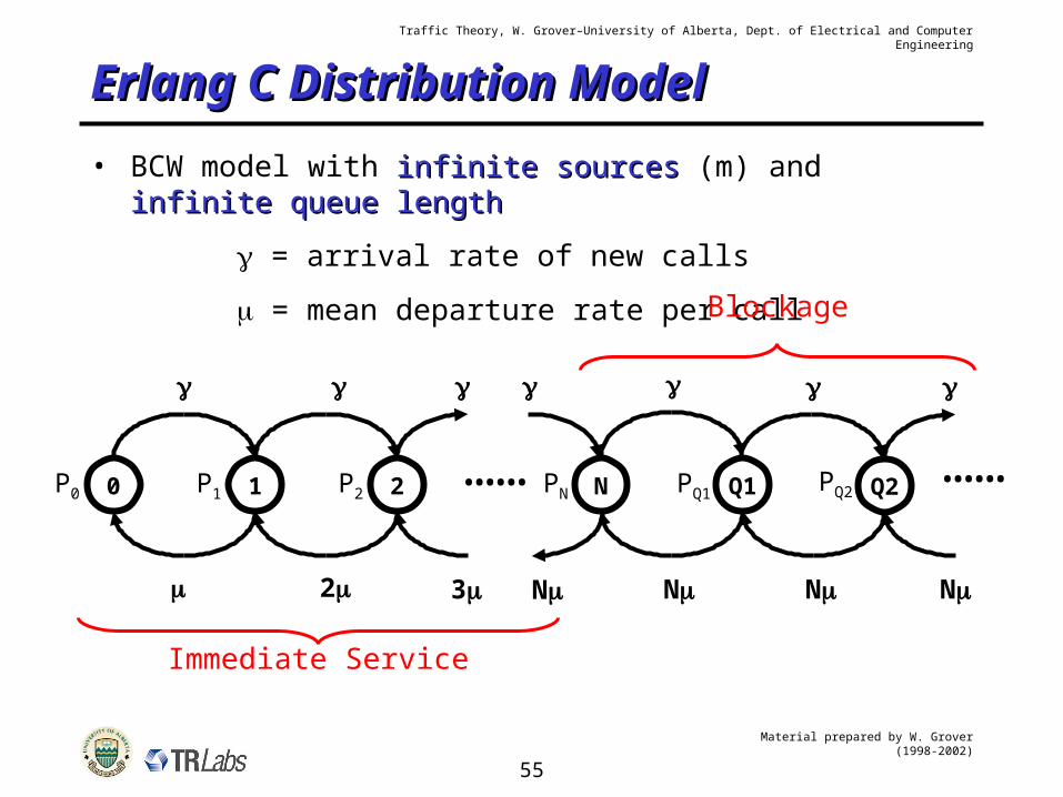
Engset Distribution ModelEngset Distribution Model
• BCC model with small number of sources (m > N)
= mean departure rate per call
= mean arrival rate of a single source
k = arrival rate if in the system is state k
kk = = (m-k)(m-k)
0 1 2 N-1 N……P0 P1 P2 PN-1 PN
m (m-1)
2
(m-2) [M-(N-2)] [m-(N-1)]
N(N-1)3
Immediate Service
Blockage
Material prepared by W. Grover (1998-2002)
53
Traffic Theory, W. Grover–University of Alberta, Dept. of Electrical and Computer Engineering
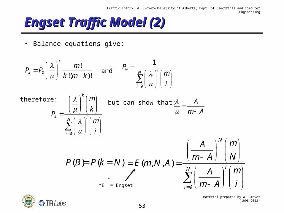
Engset Traffic Model (2)Engset Traffic Model (2)
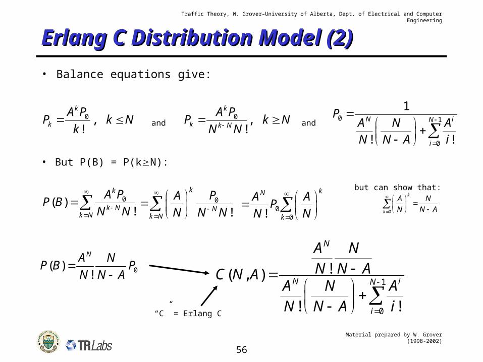
• Balance equations give:
0
!
!( )!
k
k
mP P
k m k
and 0
0
1iN
i
Pm
i
therefore:
0
k
k iN
i
m
kP
m
i
but can show that: A
m A
( ) ( )P B P k N
0
( , , )
N
iN
i
mAm A N
E m N AmA
m A i
“E” = Engset
Material prepared by W. Grover (1998-2002)
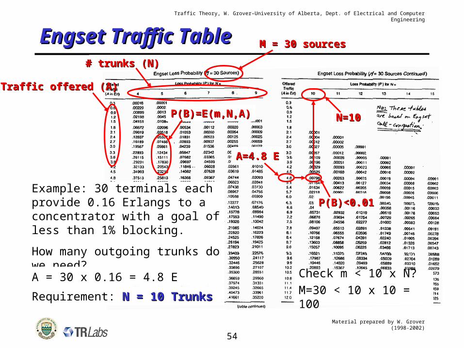
54
Traffic Theory, W. Grover–University of Alberta, Dept. of Electrical and Computer Engineering