Probability & Stochastic Processes Introduction to Probability Theory Sample Spaces Event Spaces Probability Measure Probability Functions Random Variables Moments of Random Variables Introduction to Stochastic Processes Dr Conor McArdle EE414 - Probability & Stochastic Processes 1/60
Transcript
Probability & Stochastic Processes
Introduction to Probability TheorySample SpacesEvent Spaces
Probability MeasureProbability Functions
Random VariablesMoments of Random Variables
Introduction to Stochastic Processes
Dr Conor McArdle EE414 - Probability & Stochastic Processes 1/60
Introduction to Probability Theory
Probability theory is concerned with the description and calculation of the properties ofrandom phenomena, as occur in games of chance, computer and telecommunicationssystems, financial markets, electronic and optical circuits and many other randomsystems.
Although such systems are random, in the sense that it is difficult or impossible topredict exactly how the system will behave in the future, probability theory can providecharacterisation of the type of randomness involved and yield useful measures, such asaverage values of system parameters or the likelihood of certain events occurring in thefuture.
To develop a rigorous mathematical theory of probability, the starting point is thenotion of a random experiment and an abstract probability space.
A random experiment E is an experiment satisfying the following conditions:
all possible distinct outcomes are known a priori
the outcome is not known a priori for any particular trial of the experiment
the experiment is repeatable under identical conditions
Dr Conor McArdle EE414 - Probability & Stochastic Processes 2/60
Introduction to Probability Theory
Many random phenomena can be modelled by the notion of a random experiment, forexample:
Recording the output voltage of a noise generator
Observing the daily closing price of crude oil
Measuring the number of packets queueing at the input port of a network router
Each different random experiment E defines a its own particular sample space, eventspace and probability measure, which collectively form an abstract probability space forthe random experiment.
A probability space is the collection (Ω, F , P) where
Ω the sample space is the set of all possible outcomes of a randomexperiment EF the event space is a collection of events, where each event is a subset ofthe sample space and the collection forms a σ-field
P the probability measure is an assignment of a real number in the interval[0,1] to each event in the event space.
Dr Conor McArdle EE414 - Probability & Stochastic Processes 3/60
Introduction to Probability Theory
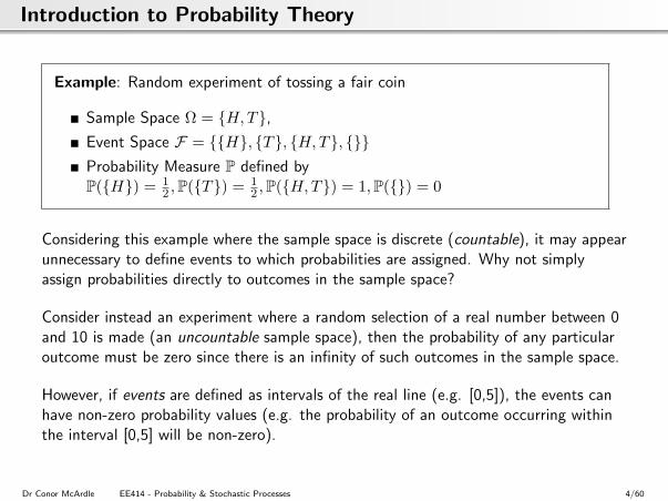
Example: Random experiment of tossing a fair coin
Sample Space Ω = H,T,Event Space F = H, T, H,T, Probability Measure P defined byP(H) = 1
2 ,P(T) = 12 ,P(H,T) = 1,P() = 0
Considering this example where the sample space is discrete (countable), it may appearunnecessary to define events to which probabilities are assigned. Why not simplyassign probabilities directly to outcomes in the sample space?
Consider instead an experiment where a random selection of a real number between 0and 10 is made (an uncountable sample space), then the probability of any particularoutcome must be zero since there is an infinity of such outcomes in the sample space.
However, if events are defined as intervals of the real line (e.g. [0,5]), the events canhave non-zero probability values (e.g. the probability of an outcome occurring withinthe interval [0,5] will be non-zero).
Dr Conor McArdle EE414 - Probability & Stochastic Processes 4/60
Introduction to Probability Theory
So that we can form a useful theory for all random experiments (particularly those withuncountable sample spaces), the probability measure is only defined on specifiedsubsets of the sample space (the events) rather than on individual outcomes in thesample space.
Note that this stipulation does not preclude us from defining events consisting of asingle outcome, but we draw the distinction between an outcome ω ∈ Ω (an element ofΩ) and an event ω ⊂ Ω (a subset of Ω).
The definition of the event space as a σ-field further specifies which subsets of Ω canbelong to the same event space. That is, there is a certain relationship between thesubsets of the sample space Ω that are chosen as events in the event space.
The properties of a σ-field (and so of any event space) ensure that if events A and Bhave probabilities defined then logical combinations of these events (e.g. the outcomeis in either A or B) are also events in the event space and so also have probabilitiesdefined. Any subset of Ω that does not belong to the event space of a randomexperiment will simply not have a defined probability.
We next look at the sample space, event space and probability measure in some detail.
Dr Conor McArdle EE414 - Probability & Stochastic Processes 5/60
Probability & Stochastic Processes
Introduction to Probability TheorySample Spaces
Event SpacesProbability Measure
Probability FunctionsRandom Variables
Moments of Random VariablesIntroduction to Stochastic Processes
Dr Conor McArdle EE414 - Probability & Stochastic Processes 6/60
Sample Spaces
A sample space Ω is the non-empty set of all outcomes (also known as samplepoints, elementary outcomes or elementary events) of a random experiment E .
The sample space takes different forms depending on the random experiment inquestion. We have seen an example of a finite sample space H,T, in the case of thecoin tossing random experiment, and also an uncountable sample space (a interval ofthe real line [0, 10]) in the case of the random number experiment.
What follows are some examples of more general sample spaces:
Example 1
A finite sample space Ω = ak : k = 1, 2, ...,K. Specific examples are:
A binary space 0, 1A finite space of integers 0, 1, 2, ..., k − 1. (Also denoted Zk).
Dr Conor McArdle EE414 - Probability & Stochastic Processes 7/60
Sample Spaces
Example 2
A countably infinite space Ω = ak : k = 1, 2, .... Specific examples are:
All non-negative integers 0, 1, 2, ..., denoted Z+
All integers ...,−2,−1, 0, 1, 2, ..., denoted Z
Example 3
An uncountably infinite space. Examples are the real line R or intervals of R such as(a, b), [a, b), (a, b], [a,∞), (−∞,∞).
Example 4
A space consisting of k-dimensional vectors with coordinates taking values in one ofthe previously described spaces. The usual name for such a vector space is a productspace. For example, let A denote one of the abstract spaces previously considered.Define the cartesian product Ak as:
Ak = (ao, a1, ..., ak−1) : ai ∈ A
Dr Conor McArdle EE414 - Probability & Stochastic Processes 8/60
Sample Spaces
Specific examples of this type of space are:
Rk
0, 1k
[a, b]k
Example 5
Let A be one of the sample spaces in examples 1-3. Form a new sample spaceconsisting of all waveforms (or functions of time) with values in A (e.g. all real valuedtime functions). This space is a product space of infinite dimension. For example:
At = all waveforms x(t) : t ∈ [0,∞) : x(t) ∈ A,∀t
Exercise 1
Specify appropriate sample spaces that model the outcomes of the following ran-dom systems: (i) tossing a coin where a head is assigned a value of 1 and a taila value of 0 (ii) rolling a die (iii) rolling three dice simultaneously (iv) choosing arandom coordinate within a cube (v) an infinite random binary waveform.
Dr Conor McArdle EE414 - Probability & Stochastic Processes 9/60
Probability & Stochastic Processes
Introduction to Probability TheorySample SpacesEvent Spaces
Probability MeasureProbability Functions
Random VariablesMoments of Random Variables
Introduction to Stochastic Processes
Dr Conor McArdle EE414 - Probability & Stochastic Processes 10/60
Event Spaces
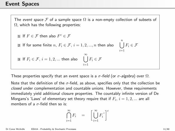
The event space F of a sample space Ω is a non-empty collection of subsets ofΩ, which has the following properties:
1 If F ∈ F then also F c ∈ F
2 If for some finite n, Fi ∈ F , i = 1, 2, ..., n then alson⋃i=1
Fi ∈ F
3 If Fi ∈ F , i = 1, 2, ... then also∞⋃i=1
Fi ∈ F
These properties specify that an event space is a σ-field (or σ-algebra) over Ω.
Note that the definition of the σ-field, as above, specifies only that the collection beclosed under complementation and countable unions. However, these requirementsimmediately yield additional closure properties. The countably infinite version of DeMorgans’s ’Laws’ of elementary set theory require that if Fi, i = 1, 2, ... are allmembers of a σ-field then so is:
∞⋂i=1
Fi =[ ∞⋃i=1
Fc
i
]cDr Conor McArdle EE414 - Probability & Stochastic Processes 11/60
Event Spaces
Thus the σ-field properties imply that the collection of events in an event space isclosed under all set-theoretic operations (union, intersection, complementation,difference, etc.) so that performing set operations on events must result in otherevents inside the event space.
This closure requirement ensures that if we know the probability of an event Aoccurring and probability of an event B occurring, then we can also find the probabilityof logical combinations such as the probability of both A and B occurring (intersectionof events), the probability of either A and B occurring (union of events), etc.
It follows by similar set-theoretic arguments that any countable sequence of any of theset-theoretic operations (union, intersection, complementation, difference, symmetricdifference, etc.) performed on events in an event space must yield other events in theevent space.
We next turn to the question of how such event spaces may be constructed.
Dr Conor McArdle EE414 - Probability & Stochastic Processes 12/60
Event Spaces: The Power Set P
Given a countable sample space Ω, the collection of all subsets of Ω is a σ-field (andthus a valid event space).
This is true since any countable sequence of set-theoretic operations on subsets of Ωmust yield another subset of Ω.
Such a collection of all possible subsets of a sample space is called the Power Set Pof the space.
The power set is the largest possible event space since it contains all subsets of Ω.
Note that, a finite sample space with n elements has a power set with at most 2n
elements.
For example, the power set of the binary sample space Ω = 0, 1 is
P = 0, 1, 0, 1,Ø with 22 elements.
Dr Conor McArdle EE414 - Probability & Stochastic Processes 13/60
Event Spaces: σ-Fields Generated by a Family of Events
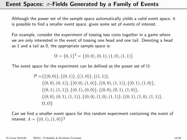
Although the power set of the sample space automatically yields a valid event space, itis possible to find a smaller event space, given some set of events of interest.
For example, consider the experiment of tossing two coins together in a game wherewe are only interested in the event of tossing one head and one tail. Denoting a headas 1 and a tail as 0, the appropriate sample space is:
Ω = 0, 12 = (0, 0), (0, 1), (1, 0), (1, 1)
The event space for the experiment can be defined as the power set of Ω:
Can we find a smaller event space for this random experiment containing the event ofinterest A = (0, 1), (1, 0)?
Dr Conor McArdle EE414 - Probability & Stochastic Processes 14/60
Event Spaces: σ-Fields Generated by a Family of Events
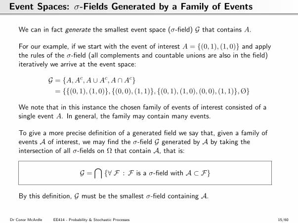
We can in fact generate the smallest event space (σ-field) G that contains A.
For our example, if we start with the event of interest A = (0, 1), (1, 0) and applythe rules of the σ-field (all complements and countable unions are also in the field)iteratively we arrive at the event space:
G = A,Ac, A ∪Ac, A ∩Ac= (0, 1), (1, 0), (0, 0), (1, 1), (0, 1), (1, 0), (0, 0), (1, 1),Ø
We note that in this instance the chosen family of events of interest consisted of asingle event A. In general, the family may contain many events.
To give a more precise definition of a generated field we say that, given a family ofevents A of interest, we may find the σ-field G generated by A by taking theintersection of all σ-fields on Ω that contain A, that is:
G =⋂∀ F : F is a σ-field with A ⊂ F
By this definition, G must be the smallest σ-field containing A.
Dr Conor McArdle EE414 - Probability & Stochastic Processes 15/60
Event Spaces
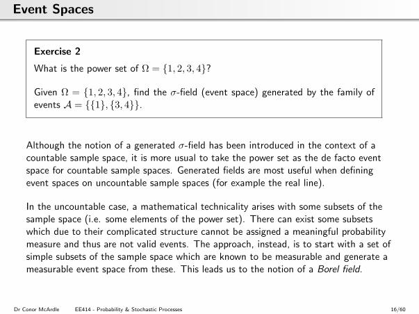
Exercise 2
What is the power set of Ω = 1, 2, 3, 4?
Given Ω = 1, 2, 3, 4, find the σ-field (event space) generated by the family ofevents A = 1, 3, 4.
Although the notion of a generated σ-field has been introduced in the context of acountable sample space, it is more usual to take the power set as the de facto eventspace for countable sample spaces. Generated fields are most useful when definingevent spaces on uncountable sample spaces (for example the real line).
In the uncountable case, a mathematical technicality arises with some subsets of thesample space (i.e. some elements of the power set). There can exist some subsetswhich due to their complicated structure cannot be assigned a meaningful probabilitymeasure and thus are not valid events. The approach, instead, is to start with a set ofsimple subsets of the sample space which are known to be measurable and generate ameasurable event space from these. This leads us to the notion of a Borel field.
Dr Conor McArdle EE414 - Probability & Stochastic Processes 16/60
Event Spaces: The Borel Field B
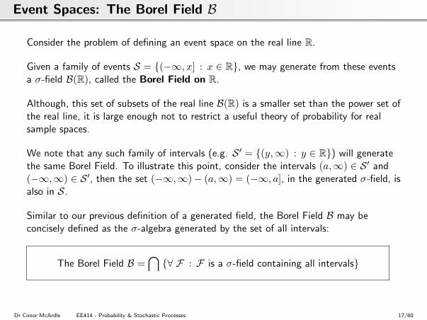
Consider the problem of defining an event space on the real line R.
Given a family of events S = (−∞, x] : x ∈ R, we may generate from these eventsa σ-field B(R), called the Borel Field on R.
Although, this set of subsets of the real line B(R) is a smaller set than the power set ofthe real line, it is large enough not to restrict a useful theory of probability for realsample spaces.
We note that any such family of intervals (e.g. S ′ = (y,∞) : y ∈ R) will generatethe same Borel Field. To illustrate this point, consider the intervals (a,∞) ∈ S ′ and(−∞,∞) ∈ S ′, then the set (−∞,∞)− (a,∞) = (−∞, a], in the generated σ-field, isalso in S.
Similar to our previous definition of a generated field, the Borel Field B may beconcisely defined as the σ-algebra generated by the set of all intervals:
The Borel Field B =⋂∀ F : F is a σ-field containing all intervals
Dr Conor McArdle EE414 - Probability & Stochastic Processes 17/60
Event Spaces: The Borel Field B
Ω = R is often a natural choice of sample space for many random systems and theBorel field B(R) on the real line is the usual choice of event space in this case.
The structure of the Borel field, being generated from intervals, makes is easier tospecify a probability measure on the set of events. By specifying probabilities on theintervals, we are assured that all events in the event space will have probabilitiesdefined.
We note that it is also possible to form a Borel field on a subset of the real line (e.g.R+). It is also possible to form a Borel field on real product spaces.
Dr Conor McArdle EE414 - Probability & Stochastic Processes 18/60
Probability & Stochastic Processes
Introduction to Probability TheorySample SpacesEvent Spaces
Probability MeasureProbability Functions
Random VariablesMoments of Random Variables
Introduction to Stochastic Processes
Dr Conor McArdle EE414 - Probability & Stochastic Processes 19/60
Probability Measure P
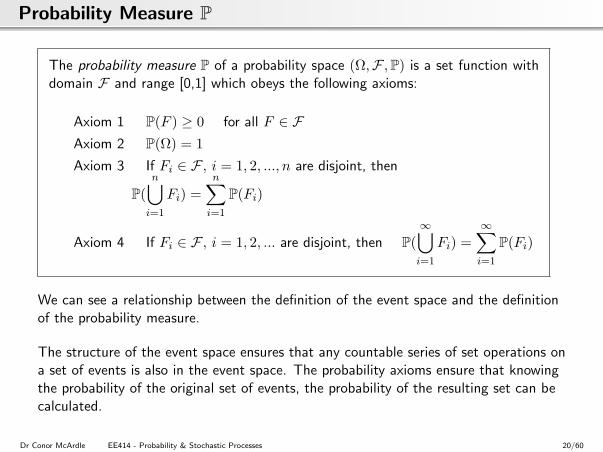
The probability measure P of a probability space (Ω,F ,P) is a set function withdomain F and range [0,1] which obeys the following axioms:
Axiom 1 P(F ) ≥ 0 for all F ∈ FAxiom 2 P(Ω) = 1Axiom 3 If Fi ∈ F , i = 1, 2, ..., n are disjoint, then
P(n⋃i=1
Fi) =n∑i=1
P(Fi)
Axiom 4 If Fi ∈ F , i = 1, 2, ... are disjoint, then P(∞⋃i=1
Fi) =∞∑i=1
P(Fi)
We can see a relationship between the definition of the event space and the definitionof the probability measure.
The structure of the event space ensures that any countable series of set operations ona set of events is also in the event space. The probability axioms ensure that knowingthe probability of the original set of events, the probability of the resulting set can becalculated.
Dr Conor McArdle EE414 - Probability & Stochastic Processes 20/60
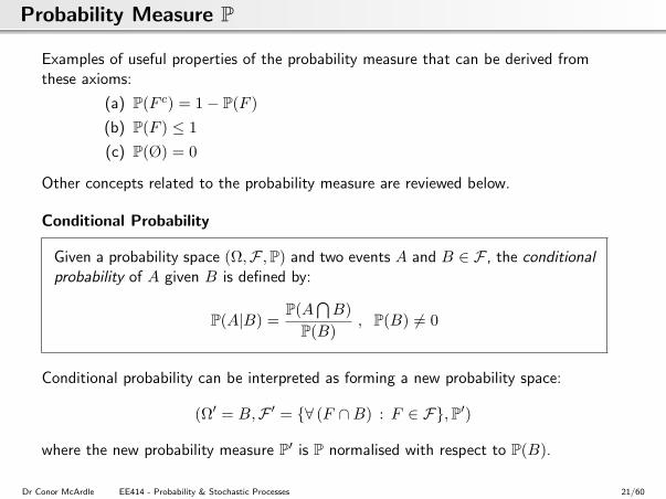
Probability Measure P
Examples of useful properties of the probability measure that can be derived fromthese axioms:
(a) P(F c) = 1− P(F )(b) P(F ) ≤ 1(c) P(Ø) = 0
Other concepts related to the probability measure are reviewed below.
Conditional Probability
Given a probability space (Ω,F ,P) and two events A and B ∈ F , the conditionalprobability of A given B is defined by:
P(A|B) =P(A
⋂B)
P(B), P(B) 6= 0
Conditional probability can be interpreted as forming a new probability space:
(Ω′ = B,F ′ = ∀ (F ∩B) : F ∈ F,P′)
where the new probability measure P′ is P normalised with respect to P(B).
Dr Conor McArdle EE414 - Probability & Stochastic Processes 21/60
Probability Measure P
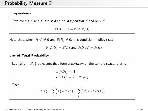
Independence
Two events A and B are said to be independent if and only if:
P(A ∩B) = P(A)P(B)
Note that, when P(A) 6= 0 and P(B) 6= 0, this condition implies that:
P(A|B) = P(A) and P(B|A) = P(B)
Law of Total Probability
Let B1, ..., Bn be events that form a partition of the sample space, that is
∪∀Bi = ΩBi ∩Bj = Ø ∀i 6= j
Then
P(A) =n∑i=1
P(A ∩Bi) =n∑i=1
P(A|Bi)P(Bi)
Dr Conor McArdle EE414 - Probability & Stochastic Processes 22/60
Probability & Stochastic Processes
Introduction to Probability TheorySample SpacesEvent Spaces
Probability MeasureProbability Functions
Random VariablesMoments of Random Variables
Introduction to Stochastic Processes
Dr Conor McArdle EE414 - Probability & Stochastic Processes 23/60
Probability Functions
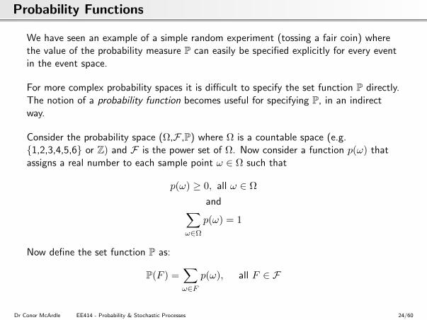
We have seen an example of a simple random experiment (tossing a fair coin) wherethe value of the probability measure P can easily be specified explicitly for every eventin the event space.
For more complex probability spaces it is difficult to specify the set function P directly.The notion of a probability function becomes useful for specifying P, in an indirectway.
Consider the probability space (Ω,F ,P) where Ω is a countable space (e.g.1,2,3,4,5,6 or Z) and F is the power set of Ω. Now consider a function p(ω) thatassigns a real number to each sample point ω ∈ Ω such that
p(ω) ≥ 0, all ω ∈ Ωand∑
ω∈Ω
p(ω) = 1
Now define the set function P as:
P(F ) =∑ω∈F
p(ω), all F ∈ F
Dr Conor McArdle EE414 - Probability & Stochastic Processes 24/60
Probability Functions
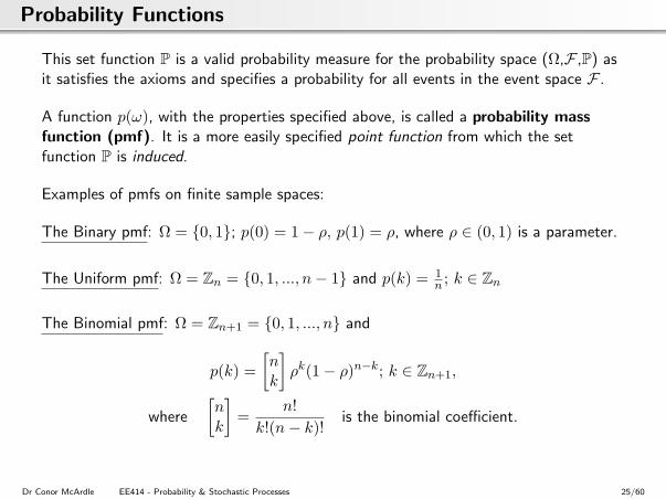
This set function P is a valid probability measure for the probability space (Ω,F ,P) asit satisfies the axioms and specifies a probability for all events in the event space F .
A function p(ω), with the properties specified above, is called a probability massfunction (pmf). It is a more easily specified point function from which the setfunction P is induced.
Examples of pmfs on finite sample spaces:
The Binary pmf: Ω = 0, 1; p(0) = 1− ρ, p(1) = ρ, where ρ ∈ (0, 1) is a parameter.
The Uniform pmf: Ω = Zn = 0, 1, ..., n− 1 and p(k) = 1n ; k ∈ Zn
The Binomial pmf: Ω = Zn+1 = 0, 1, ..., n and
p(k) =[nk
]ρk(1− ρ)n−k; k ∈ Zn+1,
where
[nk
]=
n!k!(n− k)!
is the binomial coefficient.
Dr Conor McArdle EE414 - Probability & Stochastic Processes 25/60
Probability Functions
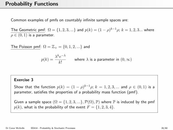
Common examples of pmfs on countably infinite sample spaces are:
The Geometric pmf: Ω = 1, 2, 3, ... and p(k) = (1− ρ)k−1ρ; k = 1, 2, 3... whereρ ∈ (0, 1) is a parameter.
The Poisson pmf: Ω = Z+ = 0, 1, 2, ... and
p(k) =λke−λ
k!where λ is a parameter in (0,∞)
Exercise 3
Show that the function p(k) = (1 − ρ)k−1ρ; k = 1, 2, 3, ... and ρ ∈ (0, 1) is aparameter, satisfies the properties of a probability mass function (pmf).
Given a sample space (Ω = 1, 2, 3, ...,P(Ω),P) where P is induced by the pmfp(k), what is the probability of the event F = 1, 2, 3, 4.
Dr Conor McArdle EE414 - Probability & Stochastic Processes 26/60
Probability Functions
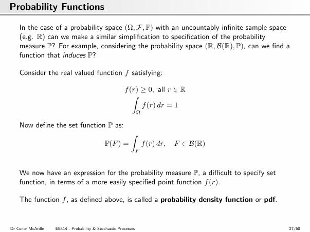
In the case of a probability space (Ω,F ,P) with an uncountably infinite sample space(e.g. R) can we make a similar simplification to specification of the probabilitymeasure P? For example, considering the probability space (R,B(R),P), can we find afunction that induces P?
Consider the real valued function f satisfying:
f(r) ≥ 0, all r ∈ R∫Ωf(r) dr = 1
Now define the set function P as:
P(F ) =∫Ff(r) dr, F ∈ B(R)
We now have an expression for the probability measure P, a difficult to specify setfunction, in terms of a more easily specified point function f(r).
The function f , as defined above, is called a probability density function or pdf.
Dr Conor McArdle EE414 - Probability & Stochastic Processes 27/60
Probability Functions
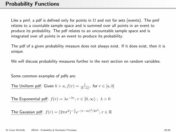
Like a pmf, a pdf is defined only for points in Ω and not for sets (events). The pmfrelates to a countable sample space and is summed over all points in an event toproduce its probability. The pdf relates to an uncountable sample space and isintegrated over all points in an event to produce its probability.
The pdf of a given probability measure does not always exist. If it does exist, then it isunique.
We will discuss probability measures further in the next section on random variables.
Some common examples of pdfs are:
The Uniform pdf: Given b > a, f(r) = 1(b−a) , for r ∈ [a, b]
The Exponential pdf: f(r) = λe−λr; r ∈ [0,∞) ; λ > 0
The Gaussian pdf: f(r) = (2πσ2)−12 e−(r−m)2/2σ2
; r ∈ R
Dr Conor McArdle EE414 - Probability & Stochastic Processes 28/60
Probability Functions
Exercise 4
Show that the exponential function f(r) = 2e−2r; r ∈ [0,∞) satisfies the prop-erties of a probability density function.
Given the probability space (R+,B(R+),P) where P is induced by the pdf f(r),find the probability of the event [0, 1].
Dr Conor McArdle EE414 - Probability & Stochastic Processes 29/60
Probability & Stochastic Processes
Introduction to Probability TheorySample SpacesEvent Spaces
Probability MeasureProbability FunctionsRandom Variables
Moments of Random VariablesIntroduction to Stochastic Processes
Dr Conor McArdle EE414 - Probability & Stochastic Processes 30/60
Random Variables: Introduction
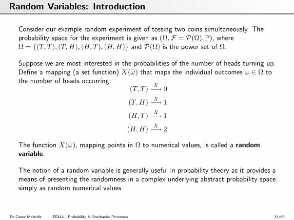
Consider our example random experiment of tossing two coins simultaneously. Theprobability space for the experiment is given as (Ω,F = P(Ω),P), whereΩ = (T, T ), (T,H), (H,T ), (H,H) and P(Ω) is the power set of Ω.
Suppose we are most interested in the probabilities of the number of heads turning up.Define a mapping (a set function) X(ω) that maps the individual outcomes ω ∈ Ω tothe number of heads occurring:
(T, T ) X−→ 0
(T,H) X−→ 1
(H,T ) X−→ 1
(H,H) X−→ 2
The function X(ω), mapping points in Ω to numerical values, is called a randomvariable.
The notion of a random variable is generally useful in probability theory as it provides ameans of presenting the randomness in a complex underlying abstract probability spacesimply as random numerical values.
Dr Conor McArdle EE414 - Probability & Stochastic Processes 31/60
Random Variables: Introduction
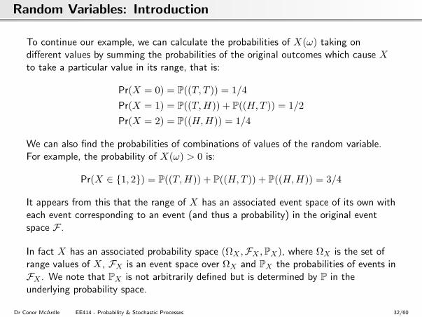
To continue our example, we can calculate the probabilities of X(ω) taking ondifferent values by summing the probabilities of the original outcomes which cause Xto take a particular value in its range, that is:
It appears from this that the range of X has an associated event space of its own witheach event corresponding to an event (and thus a probability) in the original eventspace F .
In fact X has an associated probability space (ΩX ,FX ,PX), where ΩX is the set ofrange values of X, FX is an event space over ΩX and PX the probabilities of events inFX . We note that PX is not arbitrarily defined but is determined by P in theunderlying probability space.
Dr Conor McArdle EE414 - Probability & Stochastic Processes 32/60
Random Variables: Introduction
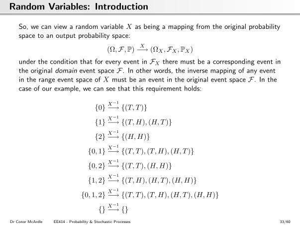
So, we can view a random variable X as being a mapping from the original probabilityspace to an output probability space:
(Ω,F ,P) X−→ (ΩX ,FX ,PX)
under the condition that for every event in FX there must be a corresponding event inthe original domain event space F . In other words, the inverse mapping of any eventin the range event space of X must be an event in the original event space F . In thecase of our example, we can see that this requirement holds:
0 X−1
−→ (T, T )
1 X−1
−→ (T,H), (H,T )
2 X−1
−→ (H,H)
0, 1 X−1
−→ (T, T ), (T,H), (H,T )
0, 2 X−1
−→ (T, T ), (H,H)
1, 2 X−1
−→ (T,H), (H,T ), (H,H)
0, 1, 2 X−1
−→ (T, T ), (T,H), (H,T ), (H,H)
X−1
−→ Dr Conor McArdle EE414 - Probability & Stochastic Processes 33/60
Random Variables
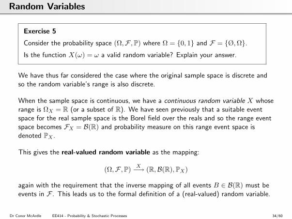
Exercise 5
Consider the probability space (Ω,F ,P) where Ω = 0, 1 and F = Ø,Ω.Is the function X(ω) = ω a valid random variable? Explain your answer.
We have thus far considered the case where the original sample space is discrete andso the random variable’s range is also discrete.
When the sample space is continuous, we have a continuous random variable X whoserange is ΩX = R (or a subset of R). We have seen previously that a suitable eventspace for the real sample space is the Borel field over the reals and so the range eventspace becomes FX = B(R) and probability measure on this range event space isdenoted PX .
This gives the real-valued random variable as the mapping:
(Ω,F ,P) X−→ (R,B(R),PX)
again with the requirement that the inverse mapping of all events B ∈ B(R) must beevents in F . This leads us to the formal definition of a (real-valued) random variable.
Dr Conor McArdle EE414 - Probability & Stochastic Processes 34/60
Random Variable: Definition
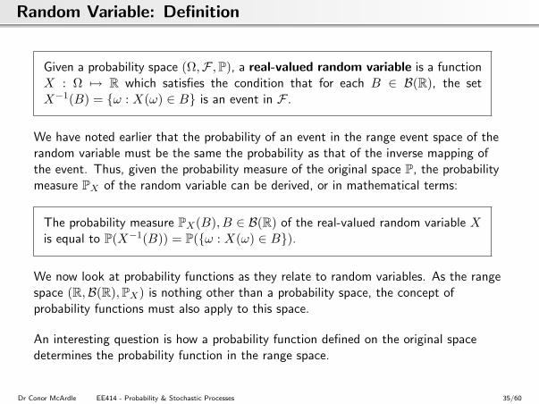
Given a probability space (Ω,F ,P), a real-valued random variable is a functionX : Ω 7→ R which satisfies the condition that for each B ∈ B(R), the setX−1(B) = ω : X(ω) ∈ B is an event in F .
We have noted earlier that the probability of an event in the range event space of therandom variable must be the same the probability as that of the inverse mapping ofthe event. Thus, given the probability measure of the original space P, the probabilitymeasure PX of the random variable can be derived, or in mathematical terms:
The probability measure PX(B), B ∈ B(R) of the real-valued random variable Xis equal to P(X−1(B)) = P(ω : X(ω) ∈ B).
We now look at probability functions as they relate to random variables. As the rangespace (R,B(R),PX) is nothing other than a probability space, the concept ofprobability functions must also apply to this space.
An interesting question is how a probability function defined on the original spacedetermines the probability function in the range space.
Dr Conor McArdle EE414 - Probability & Stochastic Processes 35/60
Discrete Random Variables and Probability Functions
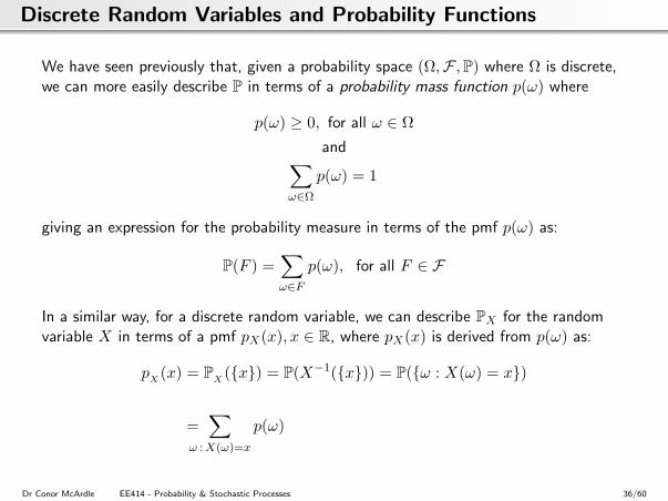
We have seen previously that, given a probability space (Ω,F ,P) where Ω is discrete,we can more easily describe P in terms of a probability mass function p(ω) where
p(ω) ≥ 0, for all ω ∈ Ωand∑
ω∈Ω
p(ω) = 1
giving an expression for the probability measure in terms of the pmf p(ω) as:
P(F ) =∑ω∈F
p(ω), for all F ∈ F
In a similar way, for a discrete random variable, we can describe PX for the randomvariable X in terms of a pmf pX(x), x ∈ R, where pX(x) is derived from p(ω) as:
pX (x) = PX (x) = P(X−1(x)) = P(ω : X(ω) = x)
=∑
ω :X(ω)=x
p(ω)
Dr Conor McArdle EE414 - Probability & Stochastic Processes 36/60
Discrete Random Variables and Probability Functions
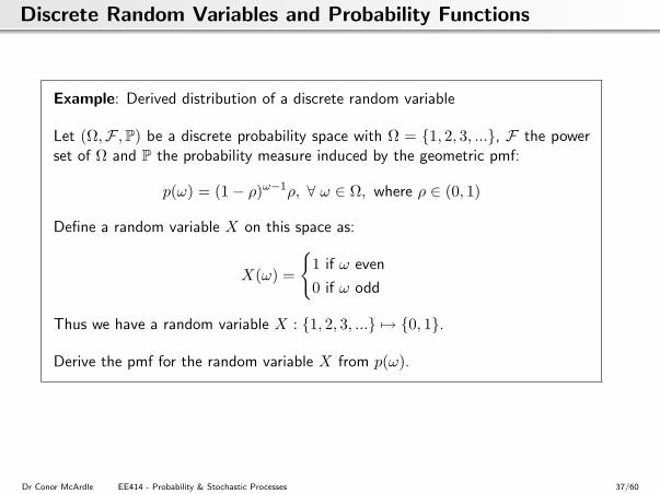
Example: Derived distribution of a discrete random variable
Let (Ω,F ,P) be a discrete probability space with Ω = 1, 2, 3, ..., F the powerset of Ω and P the probability measure induced by the geometric pmf:
p(ω) = (1− ρ)ω−1ρ, ∀ ω ∈ Ω, where ρ ∈ (0, 1)
Define a random variable X on this space as:
X(ω) =
1 if ω even
0 if ω odd
Thus we have a random variable X : 1, 2, 3, ... 7→ 0, 1.
Derive the pmf for the random variable X from p(ω).
Dr Conor McArdle EE414 - Probability & Stochastic Processes 37/60
Discrete Random Variables and Probability Functions
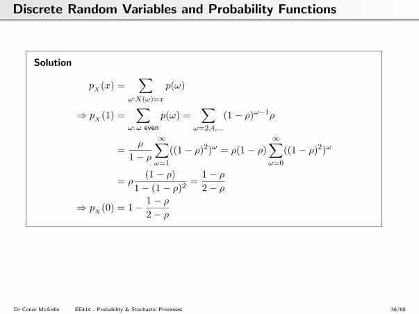
Solution
pX (x) =∑
ω:X(ω)=x
p(ω)
⇒ pX (1) =∑
ω:ω even
p(ω) =∑
ω=2,4,...
(1− ρ)ω−1ρ
=ρ
1− ρ
∞∑ω=1
((1− ρ)2)ω = ρ(1− ρ)∞∑ω=0
((1− ρ)2)ω
= ρ(1− ρ)
1− (1− ρ)2=
1− ρ2− ρ
⇒ pX (0) = 1− 1− ρ2− ρ
Dr Conor McArdle EE414 - Probability & Stochastic Processes 38/60
Continuous Random Variables and Probability Functions
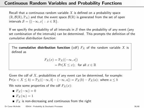
Recall that a continuous random variable X is defined on a probability space(R,B(R),PX) and that the event space B(R) is generated from the set of openintervals S = (−∞, x] : x ∈ R.
If we specify the probability of all intervals in S then the probability of any event (anyset combination of the intervals) can be determined. This prompts the definition of thecumulative distribution function:
The cumulative distribution function (cdf) FX of the random variable X isdefined as
FX(x) = PX((−∞, x])= Pr(X ≤ x); for all x ∈ R
Given the cdf of X, probabilities of any event can be determined, for example:Pr(a < X ≤ b) = PX((−∞, b]− (−∞, a]) = FX(b)− FX(a); where a ≤ bWe note some properties of the cdf FX(x):
FX(−∞) = 0FX(∞) = 1FX is non-decreasing and continuous from the right
Dr Conor McArdle EE414 - Probability & Stochastic Processes 39/60
Continuous Random Variables and Probability Functions
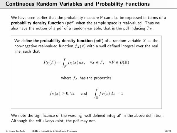
We have seen earlier that the probability measure P can also be expressed in terms of aprobability density function (pdf) when the sample space is real-valued. Thus wealso have the notion of a pdf of a random variable, that is the pdf inducing PX .
We define the probability density function (pdf) of a random variable X as thenon-negative real-valued function fX(x) with a well defined integral over the realline, such that
PX(F ) =∫FfX(x) dx, ∀x ∈ F, ∀F ∈ B(R)
where fX has the properties
fX(x) ≥ 0,∀x and
∫RfX(x) dx = 1
We note the significance of the wording ’well defined integral’ in the above definition.Although the cdf always exist, the pdf may not.
Dr Conor McArdle EE414 - Probability & Stochastic Processes 40/60
Continuous Random Variables and Probability Functions
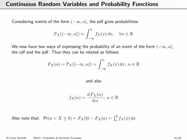
Considering events of the form (−∞, α], the pdf gives probabilities:
PX((−∞, α]) =∫ α
−∞fX(x) dx, ∀α ∈ R
We now have two ways of expressing the probability of an event of the form (−∞, α],the cdf and the pdf. Thus they can be related as follows:
FX(α) = PX((−∞, α]) =∫ α
−∞fX(x) dx; α ∈ R
and also
fX(α) =dFX(α)dα
; α ∈ R
Also note that: Pr(a < X ≤ b) = FX(b)− FX(a) =∫ ba fX(x) dx
Dr Conor McArdle EE414 - Probability & Stochastic Processes 41/60
Continuous Random Variables and Probability Functions
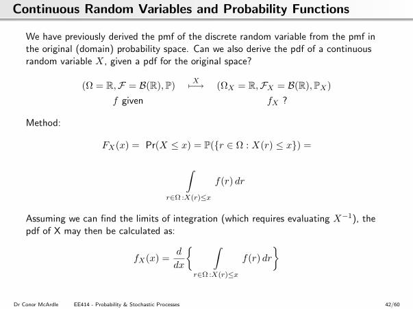
We have previously derived the pmf of the discrete random variable from the pmf inthe original (domain) probability space. Can we also derive the pdf of a continuousrandom variable X, given a pdf for the original space?
(Ω = R,F = B(R),P) X7−→ (ΩX = R,FX = B(R),PX)f given fX ?
Method:
FX(x) = Pr(X ≤ x) = P(r ∈ Ω : X(r) ≤ x) =
∫r∈Ω :X(r)≤x
f(r) dr
Assuming we can find the limits of integration (which requires evaluating X−1), thepdf of X may then be calculated as:
fX(x) =d
dx
∫r∈Ω :X(r)≤x
f(r) dr
Dr Conor McArdle EE414 - Probability & Stochastic Processes 42/60
Continuous Random Variables and Probability Functions
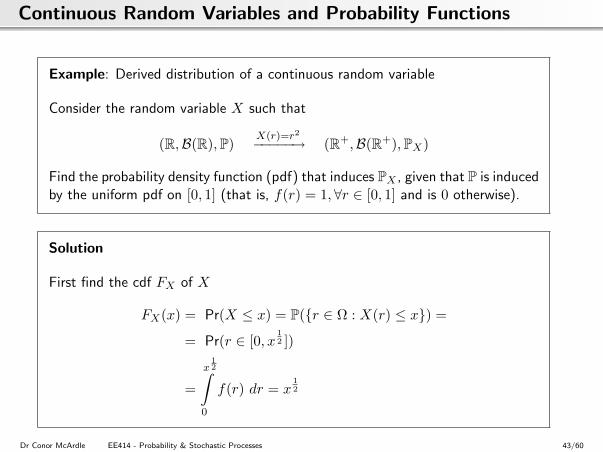
Example: Derived distribution of a continuous random variable
Consider the random variable X such that
(R,B(R),P)X(r)=r2−−−−−→ (R+,B(R+),PX)
Find the probability density function (pdf) that induces PX , given that P is inducedby the uniform pdf on [0, 1] (that is, f(r) = 1,∀r ∈ [0, 1] and is 0 otherwise).
Solution
First find the cdf FX of X
FX(x) = Pr(X ≤ x) = P(r ∈ Ω : X(r) ≤ x) =
= Pr(r ∈ [0, x12 ])
=
x12∫
0
f(r) dr = x12
Dr Conor McArdle EE414 - Probability & Stochastic Processes 43/60
Continuous Random Variables and Probability Functions
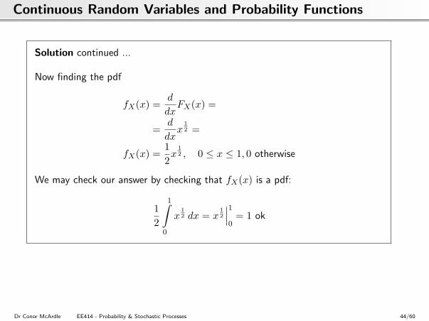
Solution continued ...
Now finding the pdf
fX(x) =d
dxFX(x) =
=d
dxx
12 =
fX(x) =12x
12 , 0 ≤ x ≤ 1, 0 otherwise
We may check our answer by checking that fX(x) is a pdf:
12
1∫0
x12 dx = x
12
∣∣∣10
= 1 ok
Dr Conor McArdle EE414 - Probability & Stochastic Processes 44/60
Probability & Stochastic Processes
Introduction to Probability TheorySample SpacesEvent Spaces
Probability MeasureProbability Functions
Random VariablesMoments of Random Variables
Introduction to Stochastic Processes
Dr Conor McArdle EE414 - Probability & Stochastic Processes 45/60
Moments of Random Variables: Expectation
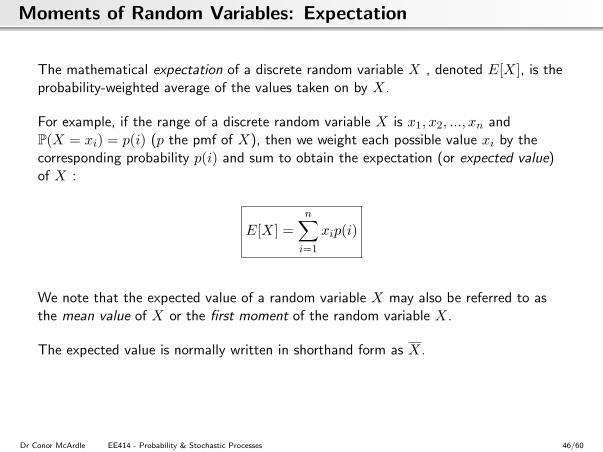
The mathematical expectation of a discrete random variable X , denoted E[X], is theprobability-weighted average of the values taken on by X.
For example, if the range of a discrete random variable X is x1, x2, ..., xn andP(X = xi) = p(i) (p the pmf of X), then we weight each possible value xi by thecorresponding probability p(i) and sum to obtain the expectation (or expected value)of X :
E[X] =n∑i=1
xip(i)
We note that the expected value of a random variable X may also be referred to asthe mean value of X or the first moment of the random variable X.
The expected value is normally written in shorthand form as X.
Dr Conor McArdle EE414 - Probability & Stochastic Processes 46/60
Moments of Random Variables: Expectation
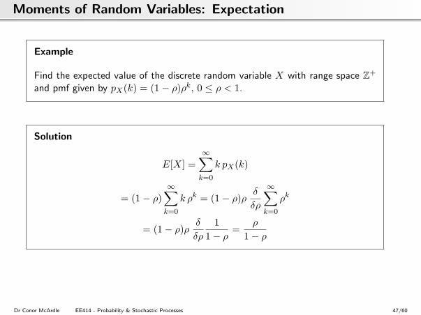
Example
Find the expected value of the discrete random variable X with range space Z+
and pmf given by pX(k) = (1− ρ)ρk, 0 ≤ ρ < 1.
Solution
E[X] =∞∑k=0
k pX(k)
= (1− ρ)∞∑k=0
k ρk = (1− ρ)ρδ
δρ
∞∑k=0
ρk
= (1− ρ)ρδ
δρ
11− ρ
=ρ
1− ρ
Dr Conor McArdle EE414 - Probability & Stochastic Processes 47/60
Moments of Random Variables: Expectation
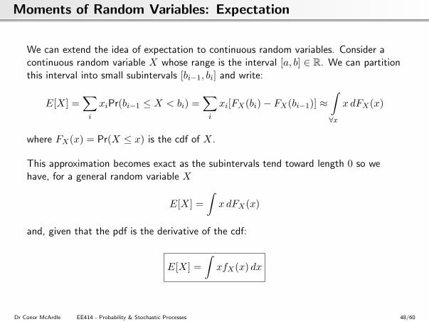
We can extend the idea of expectation to continuous random variables. Consider acontinuous random variable X whose range is the interval [a, b] ∈ R. We can partitionthis interval into small subintervals [bi−1, bi] and write:
E[X] =∑i
xiPr(bi−1 ≤ X < bi) =∑i
xi[FX(bi)− FX(bi−1)] ≈∫∀x
x dFX(x)
where FX(x) = Pr(X ≤ x) is the cdf of X.
This approximation becomes exact as the subintervals tend toward length 0 so wehave, for a general random variable X
E[X] =∫x dFX(x)
and, given that the pdf is the derivative of the cdf:
E[X] =∫xfX(x) dx
Dr Conor McArdle EE414 - Probability & Stochastic Processes 48/60
Moments of Random Variables: Expectation
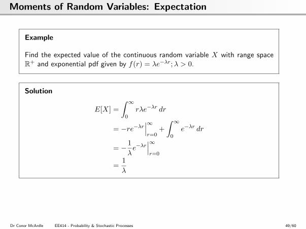
Example
Find the expected value of the continuous random variable X with range spaceR+ and exponential pdf given by f(r) = λe−λr;λ > 0.
Solution
E[X] =∫ ∞
0rλe−λr dr
= −re−λr∣∣∣∞r=0
+∫ ∞
0e−λr dr
= − 1λe−λr
∣∣∣∞r=0
=1λ
Dr Conor McArdle EE414 - Probability & Stochastic Processes 49/60
Moments of Random Variables: Variance
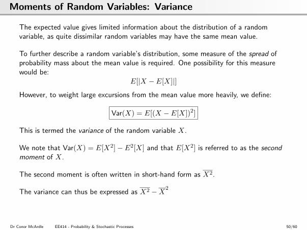
The expected value gives limited information about the distribution of a randomvariable, as quite dissimilar random variables may have the same mean value.
To further describe a random variable’s distribution, some measure of the spread ofprobability mass about the mean value is required. One possibility for this measurewould be:
E[|X − E[X]|]
However, to weight large excursions from the mean value more heavily, we define:
Var(X) = E[(X − E[X])2]
This is termed the variance of the random variable X.
We note that Var(X) = E[X2]− E2[X] and that E[X2] is referred to as the secondmoment of X.
The second moment is often written in short-hand form as X2.
The variance can thus be expressed as X2 −X2
Dr Conor McArdle EE414 - Probability & Stochastic Processes 50/60
Moments of Random Variables: Variance
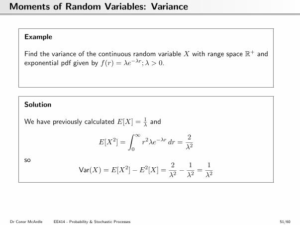
Example
Find the variance of the continuous random variable X with range space R+ andexponential pdf given by f(r) = λe−λr;λ > 0.
Solution
We have previously calculated E[X] = 1λ and
E[X2] =∫ ∞
0r2λe−λr dr =
2λ2
so
Var(X) = E[X2]− E2[X] =2λ2− 1λ2
=1λ2
Dr Conor McArdle EE414 - Probability & Stochastic Processes 51/60
Probability & Stochastic Processes
Introduction to Probability TheorySample SpacesEvent Spaces
Probability MeasureProbability Functions
Random VariablesMoments of Random Variables
Introduction to Stochastic Processes
Dr Conor McArdle EE414 - Probability & Stochastic Processes 52/60
Stochastic Processes
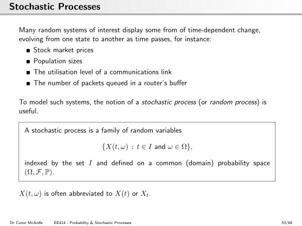
Many random systems of interest display some from of time-dependent change,evolving from one state to another as time passes, for instance:
Stock market prices
Population sizes
The utilisation level of a communications link
The number of packets queued in a router’s buffer
To model such systems, the notion of a stochastic process (or random process) isuseful.
A stochastic process is a family of random variables
X(t, ω) : t ∈ I and ω ∈ Ω,
indexed by the set I and defined on a common (domain) probability space(Ω,F ,P).
X(t, ω) is often abbreviated to X(t) or Xt.
Dr Conor McArdle EE414 - Probability & Stochastic Processes 53/60
Stochastic Processes
The index set I may be discrete (e.g. I = Z+) or continuous (e.g. I = [0,∞)). I isusually interpreted as being time (either discrete or continuous).
We can view a stochastic process as being a mapping from each sample point ω ∈ Ωto a function of time and note that:
For a given value of ω, X(t, ω) is a function of time,
For a given value of t, X(t, ω) is a random variable and
For a given value of both ω and t, X(t, ω) is a fixed sample value.
X(t, ω) for a given ω is also called a trajectory or sample path of the random process.We observe that the probability distribution governing the likelihood of different ω’sdictates the likelihood of different trajectories that the output value of the stochasticprocess will take over time.
We also observe that, at a given time t, X(t, ω) describes the likelihood of differentvalues (states) of the process. That is, at a given point in time (e.g. t = t1), therandom variable X(t1, ω) has a cdf (or pmf if discrete) describing the likelihood of theprocess being in different states at that time.
Dr Conor McArdle EE414 - Probability & Stochastic Processes 54/60
Stochastic Processes
Example of a Stochastic Process
Consider a game where a coin is tossed repeatedly (ad infinitum) and the player’s scoreis accumulated by adding 1 point when a head turns up and deducting 1 point when atail turns up. Let us describe this process as a stochastic process defined on a commonprobability space (Ω,F ,P).
A single outcome of the experiment is some infinite sequence of equally likely 1’s and-1’s, that is the sample space is a product space:
Ω = −1, 1∞ = all vectors ω = (a0, a1, ..., ai, ...) : ai ∈ −1, 1
We can then describe the player’s score as the stochastic process:
X(t, ω) =t∑i=0
ai, t ∈ Z+, ai the i’th component of ω ∈ Ω
We note that at any fixed value of t ∈ Z+, we have a random variable. For example,X(2, ω) is a random variable with associated pmf:
X(2,−2) =14, X(2, 0) =
12, X(2, 2) =
14
Dr Conor McArdle EE414 - Probability & Stochastic Processes 55/60
Stochastic Processes: Classifications
Stochastic processes may be classified according to the nature of:
1 The State Space, the set of possible values (or states) that X(t, ω) can take on.The state space can either be (i) discrete (finite or countable set of states) or (ii)continuous (values over continuous intervals).
2 The Parameter Space, the permitted times at which changes in state may occur.The parameter space can either be (i) discrete (discrete time process) or (ii)continuous (continuous time process).
3 The Statistical Dependencies among the the family of random variablesX(t, ω), for different values of t. Classifications of statistical dependencies arediscussed below.
Dr Conor McArdle EE414 - Probability & Stochastic Processes 56/60
Stochastic Processes: Classifications
Statistical Dependencies
Firstly let us consider possible probabilistic relationships between two random variablesX and Y . Consider the events (X ≤ x) and (Y ≤ y). The events are independent if
Pr((X ≤ x) and (Y ≤ y)) = Pr(X ≤ x).Pr(Y ≤ y)
Where this is not the case, there is a statistical dependency between the events.
The random variables X and Y are said to be independent if
Pr((X ≤ x) and (Y ≤ y)) = Pr(X ≤ x).Pr(Y ≤ y)for all such events (X ≤ x) and (Y ≤ y)
Where this is not the case, the probabilistic dependencies between X and Y can bedescribed in terms of joint probability functions.
Dr Conor McArdle EE414 - Probability & Stochastic Processes 57/60
Stochastic Processes: Statistical Dependencies
The joint distribution function of random variables X and Y is defined as
FX,Y (x, y) = Pr(X ≤ x, Y ≤ y)
The joint probability density function of random variables X and Y is defined as
fX,Y (x, y) =δ
δx
δ
δyFX,Y (x, y)
We observe an alternative definition of independence. X and Y are independent if
FX,Y (x, y) = FX(x)FY (y)
or, equivalently, X and Y are independent if
fX,Y (x, y) = fX(x)fY (y)
Dr Conor McArdle EE414 - Probability & Stochastic Processes 58/60
Stochastic Processes: Statistical Dependencies
The the notion of joint distributions and joint density functions can be extended to agroup of any number of random variables.
Consider the the stochastic process X(t, ω) as an infinite series of random variablesX(ti, ω) where i ∈ I an infinite index set. The the joint distribution function of theserandom variables can be denoted:
We note that independent processes are somewhat trivial, given that the state of theprocess does not evolve from (depend on) previous states. For (more interesting)process that are not independent, the statistical dependence between states at differenttimes is expressed in the joint distribution function, however, in general, this function iscomplex and so simpler mechanisms of specification are more useful.
We will see an example of such a mechanism when we meet Markov Processes.
Dr Conor McArdle EE414 - Probability & Stochastic Processes 59/60
Stochastic Processes: Statistical Dependencies
Other classifications of stochastic processes relating to statistical dependencies can bemade:
A Stationary Process is a stochastic process whose joint distribution functionFX(t1),X(t2),... does not change with shifts in time, that is, for a constant τ ,
FX(t1+τ),X(t2+τ),... = FX(t1),X(t2),...
An Ergodic Process is a stochastic process where a full description of the process canbe determined from a single (infinitely long) sample path of the process. This infersthat the behaviour of the process, after a long period of evolution, becomesindependent of the starting point of the process.
Exercise 6
Give a classification of the stochastic process described in the previous example(the infinite coin tossing game).
Dr Conor McArdle EE414 - Probability & Stochastic Processes 60/60