Page 1
EE465: Introduction to Digital Image Processing 1
Introduction to Grayscale and Color Images
Image acquisitionLight and Electromagnetic spectrumCharge-Coupled Device (CCD) imaging and Bayer
Pattern (the most popular color-filter-array)Sampling and Quantization
Image representationSpatial resolutionBit-depth resolutionLocal neighborhoodBlock decomposition
Page 2
EE465: Introduction to Digital Image Processing 2
Electromagnetic spectrum
Page 3
EE465: Introduction to Digital Image Processing 3
Light: the Visible Spectrum
Visible range: 0.43µm(violet)-0.78µm(red)Six bands: violet, blue, green, yellow,
orange, redThe color of an object is determined by the
nature of the light reflected by the objectMonochromatic light (gray level)Three elements measuring chromatic light
Radiance, luminance and brightness
Page 4
EE465: Introduction to Digital Image Processing 4
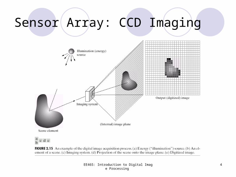
Sensor Array: CCD Imaging
Page 5
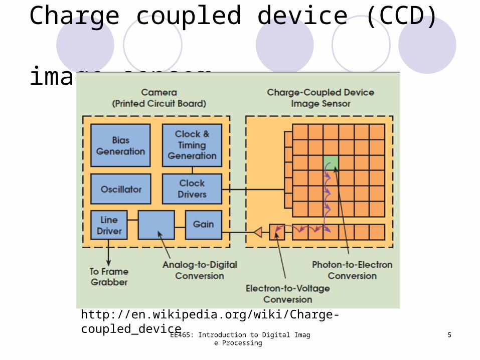
Charge coupled device (CCD) image sensor
EE465: Introduction to Digital Image Processing 5
http://en.wikipedia.org/wiki/Charge-coupled_device
Page 6
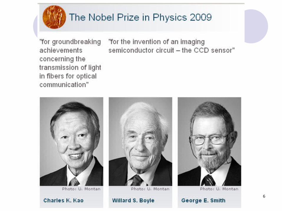
EE465: Introduction to Digital Image Processing 6
Page 7
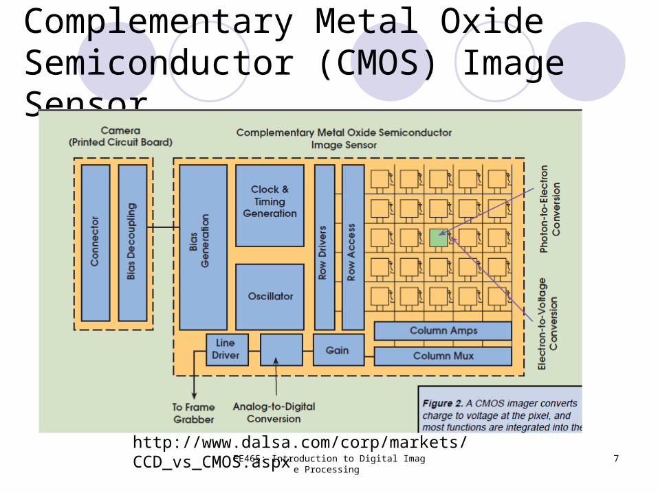
Complementary Metal Oxide Semiconductor (CMOS) Image Sensor
EE465: Introduction to Digital Image Processing 7
http://www.dalsa.com/corp/markets/CCD_vs_CMOS.aspx
Page 8
EE465: Introduction to Digital Image Processing 8
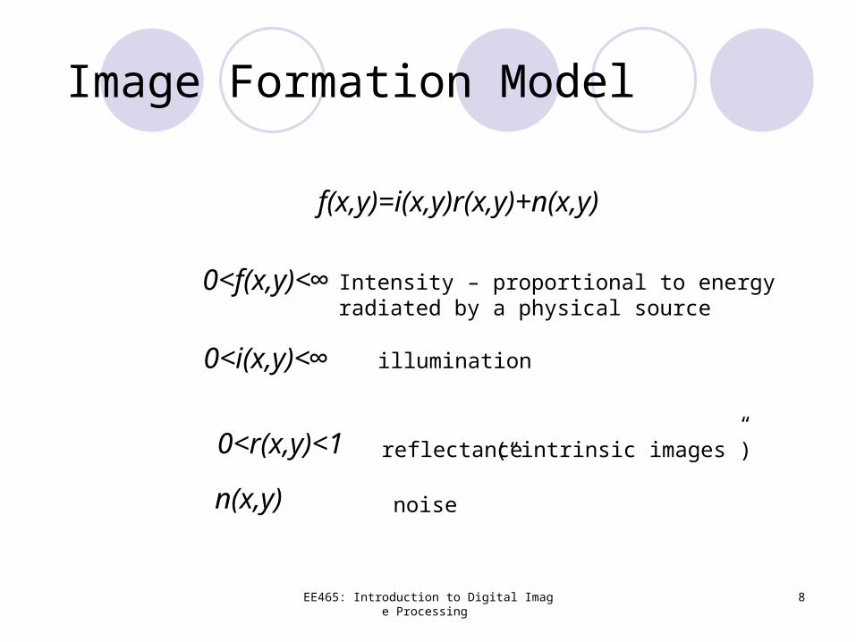
Image Formation Model
f(x,y)=i(x,y)r(x,y)+n(x,y)
0<f(x,y)<∞
0<i(x,y)<∞
0<r(x,y)<1 reflectance
illumination
Intensity – proportional to energyradiated by a physical source
(“intrinsic images”)
n(x,y) noise
Page 9
EE465: Introduction to Digital Image Processing 9
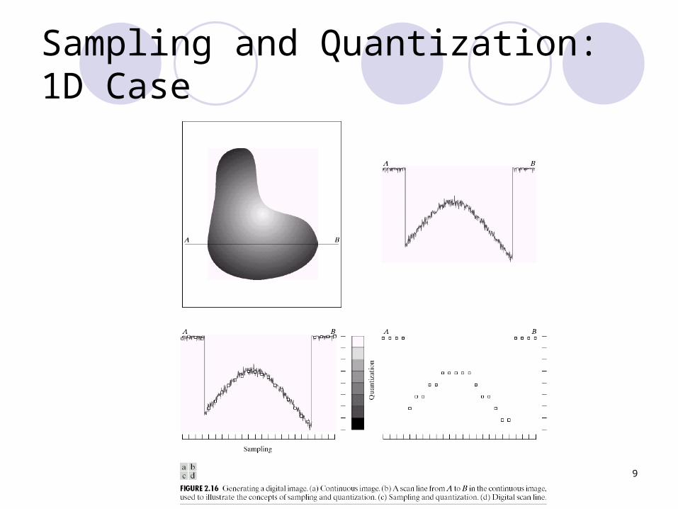
Sampling and Quantization: 1D Case
Page 10
EE465: Introduction to Digital Image Processing 10
2D Sampling and Quantization
Page 11
EE465: Introduction to Digital Image Processing 11
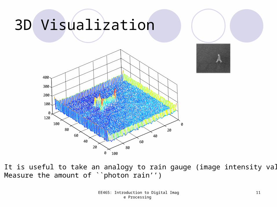
3D Visualization
0
20
40
60
80
100
120
0
20
40
60
80
100
0
100
200
300
400
It is useful to take an analogy to rain gauge (image intensity valuesMeasure the amount of ``photon rain’’)
Page 12
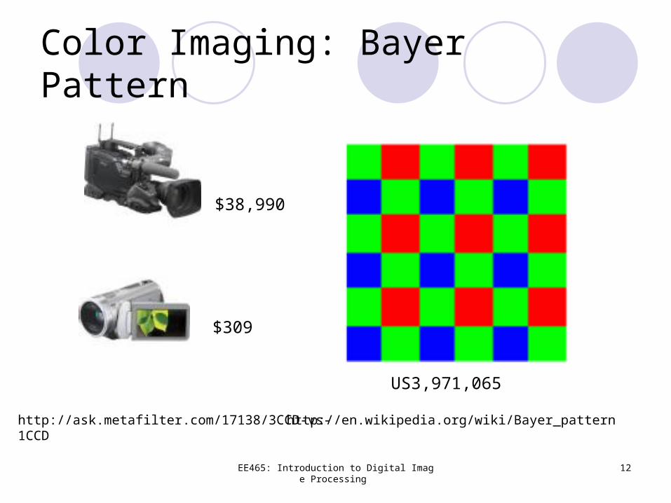
Color Imaging: Bayer Pattern
EE465: Introduction to Digital Image Processing 12
US3,971,065
http://en.wikipedia.org/wiki/Bayer_patternhttp://ask.metafilter.com/17138/3CCD-vs-1CCD
$38,990
$309
Page 13
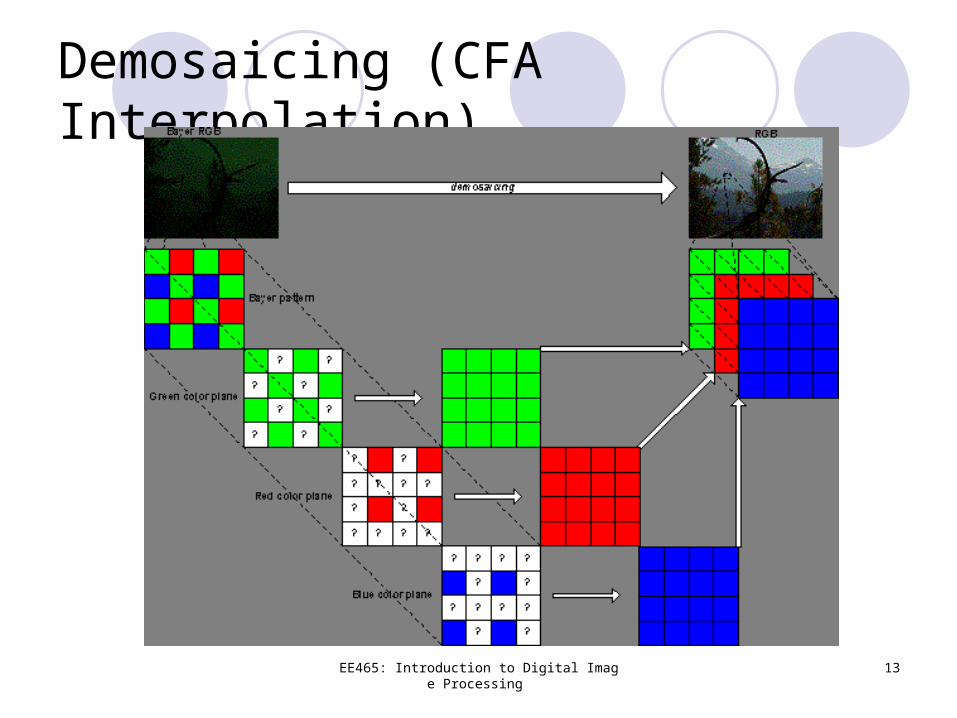
Demosaicing (CFA Interpolation)
EE465: Introduction to Digital Image Processing 13
Page 14
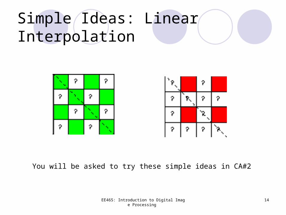
Simple Ideas: Linear Interpolation
EE465: Introduction to Digital Image Processing 14
You will be asked to try these simple ideas in CA#2
Page 15
Biological vs. Artificial Sensors
EE465: Introduction to Digital Image Processing 15
US3,971,065 Cone distribution in human retina
Question: Engineers’ invention vs. nature’s evolution, who wins?
Page 16
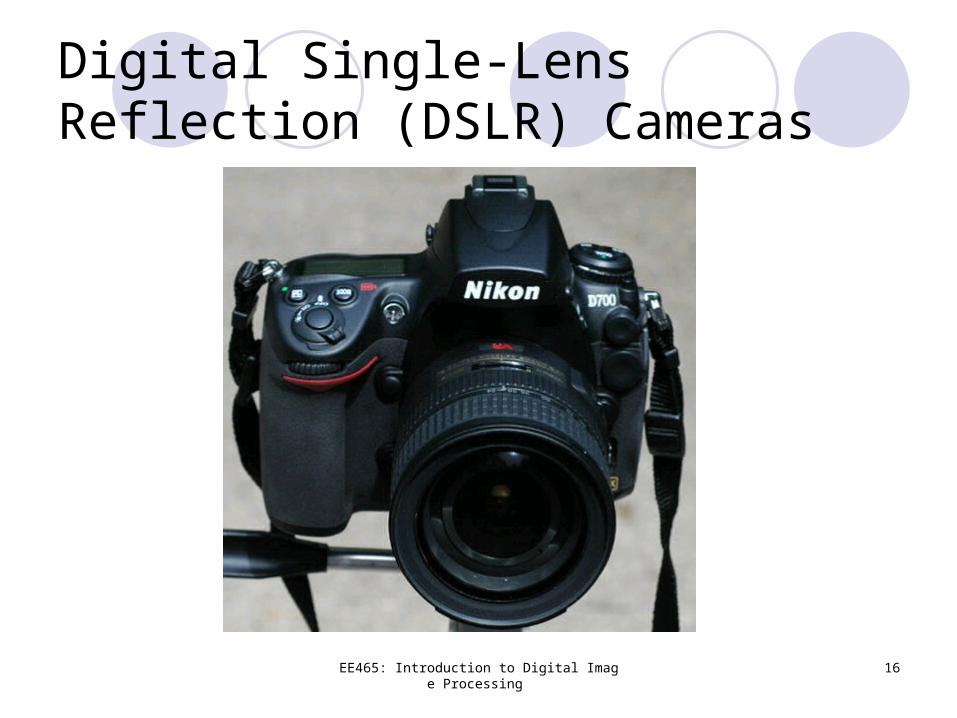
Digital Single-Lens Reflection (DSLR) Cameras
EE465: Introduction to Digital Image Processing 16
Page 17
EE465: Introduction to Digital Image Processing 17
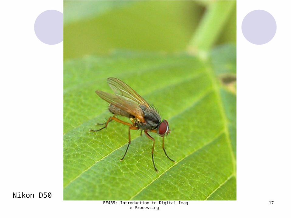
Nikon D50
Page 18
EE465: Introduction to Digital Image Processing 18
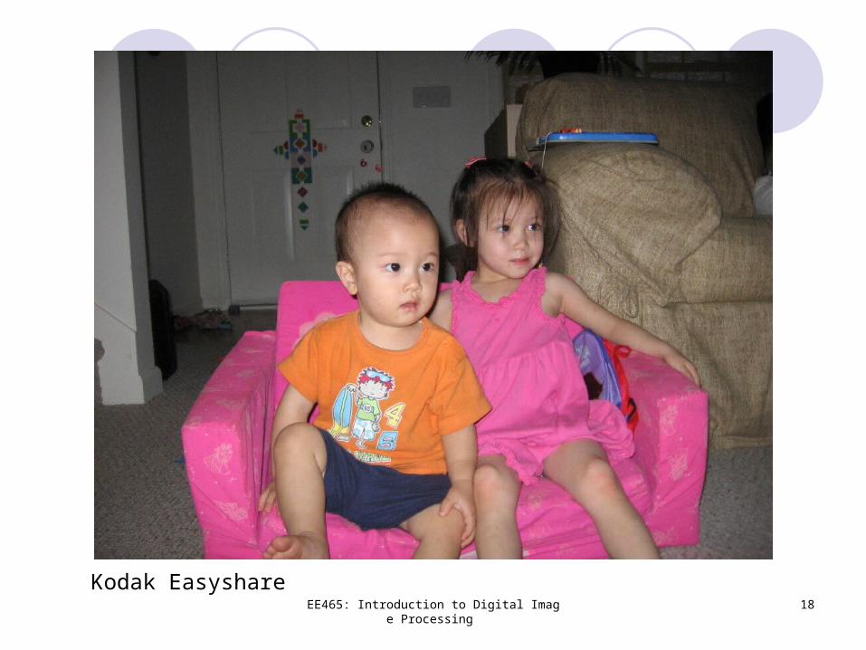
Kodak Easyshare
Page 19
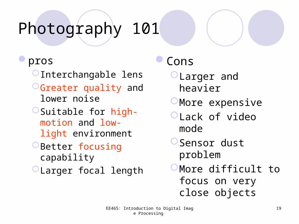
Photography 101
prosInterchangable lensGreater quality and
lower noiseSuitable for high-
motion and low-light environment
Better focusing capability
Larger focal length
ConsLarger and heavierMore expensiveLack of video modeSensor dust problemMore difficult to focus
on very close objects
EE465: Introduction to Digital Image Processing 19
Page 20
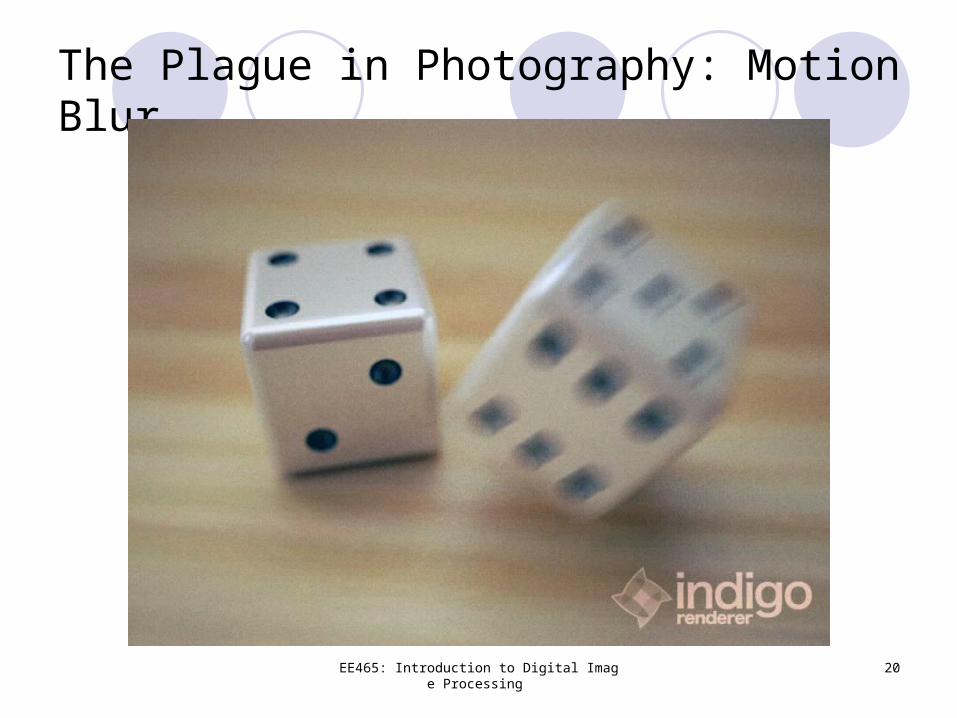
The Plague in Photography: Motion Blur
EE465: Introduction to Digital Image Processing 20
Page 21
EE465: Introduction to Digital Image Processing 21
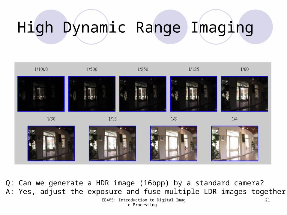
High Dynamic Range Imaging
Q: Can we generate a HDR image (16bpp) by a standard camera?A: Yes, adjust the exposure and fuse multiple LDR images together
Page 22
EE465: Introduction to Digital Image Processing 22
HDR Display (After Toner Mapping)
Note that any commercial display devices we see these days are NOT HDR
Page 23
EE465: Introduction to Digital Image Processing 23
Page 24
EE465: Introduction to Digital Image Processing 24
Beyond Visible
Gamma-ray and X-ray: medical and astronomical applications
Infrared (thermal imaging): near-infrared and far-infrared
Microwave imaging: Radio-frequency: MRI and astronomic
applications
Page 25
EE465: Introduction to Digital Image Processing 25
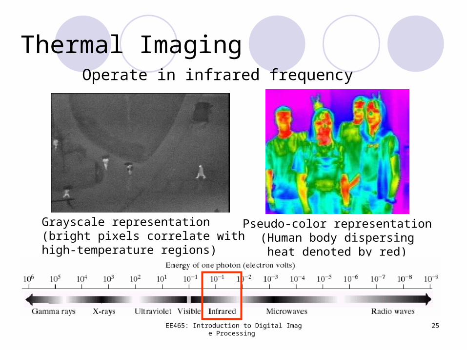
Thermal Imaging
Pseudo-color representation(Human body dispersing
heat denoted by red)
Operate in infrared frequency
Grayscale representation(bright pixels correlate withhigh-temperature regions)
Page 26
EE465: Introduction to Digital Image Processing 26
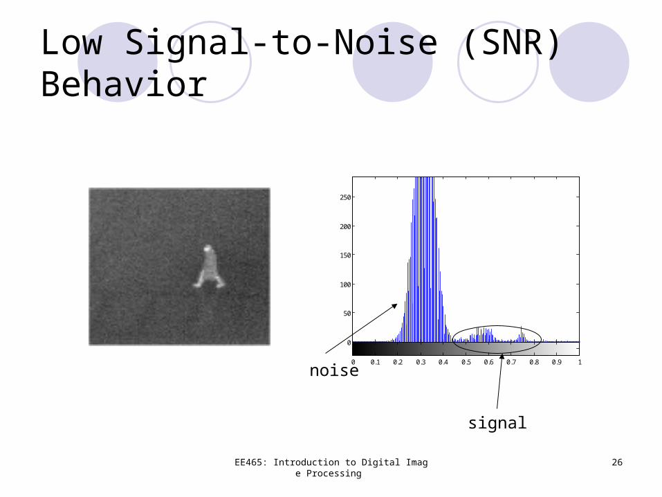
Low Signal-to-Noise (SNR) Behavior
0 0.1 0.2 0.3 0.4 0.5 0.6 0.7 0.8 0.9 1
0
50
100
150
200
250
noise
signal
Page 27
EE465: Introduction to Digital Image Processing 27
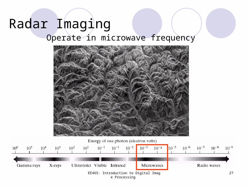
Radar Imaging
Mountains in Southeast Tibet
Operate in microwave frequency
Page 28
EE465: Introduction to Digital Image Processing 28
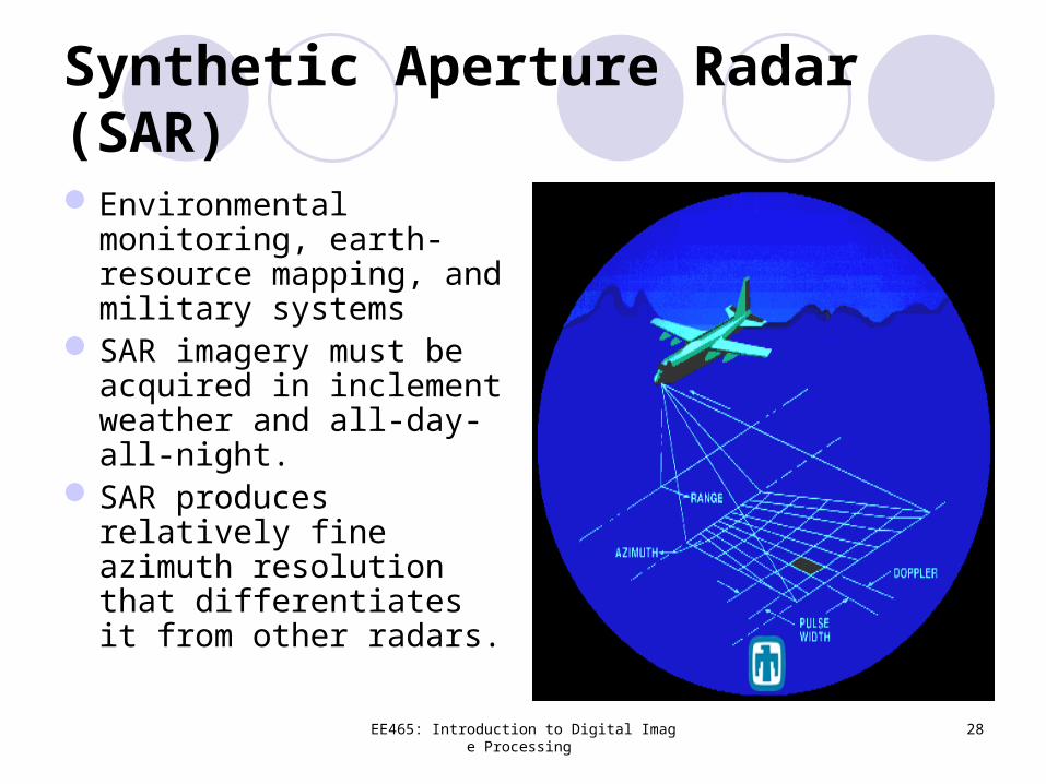
Synthetic Aperture Radar (SAR)Environmental
monitoring, earth-resource mapping, and military systems
SAR imagery must be acquired in inclement weather and all-day-all-night.
SAR produces relatively fine azimuth resolution that differentiates it from other radars.
Page 29
EE465: Introduction to Digital Image Processing 29
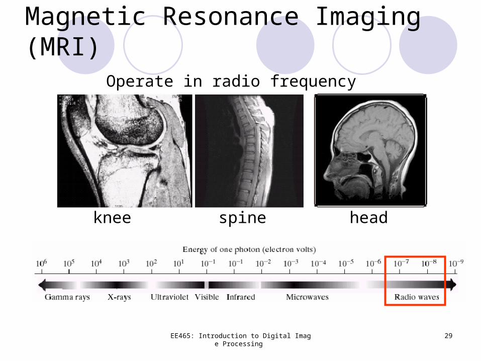
Magnetic Resonance Imaging (MRI)
knee spine head
Operate in radio frequency
Page 30
EE465: Introduction to Digital Image Processing 30
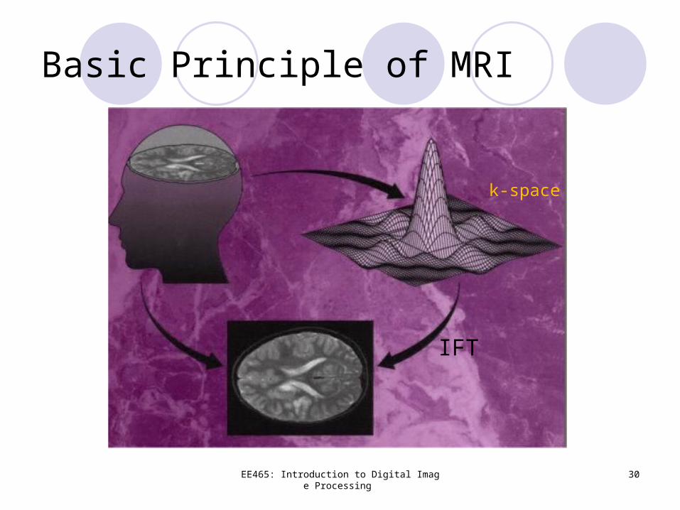
Basic Principle of MRI
IFT
k-space
Page 31
EE465: Introduction to Digital Image Processing 31
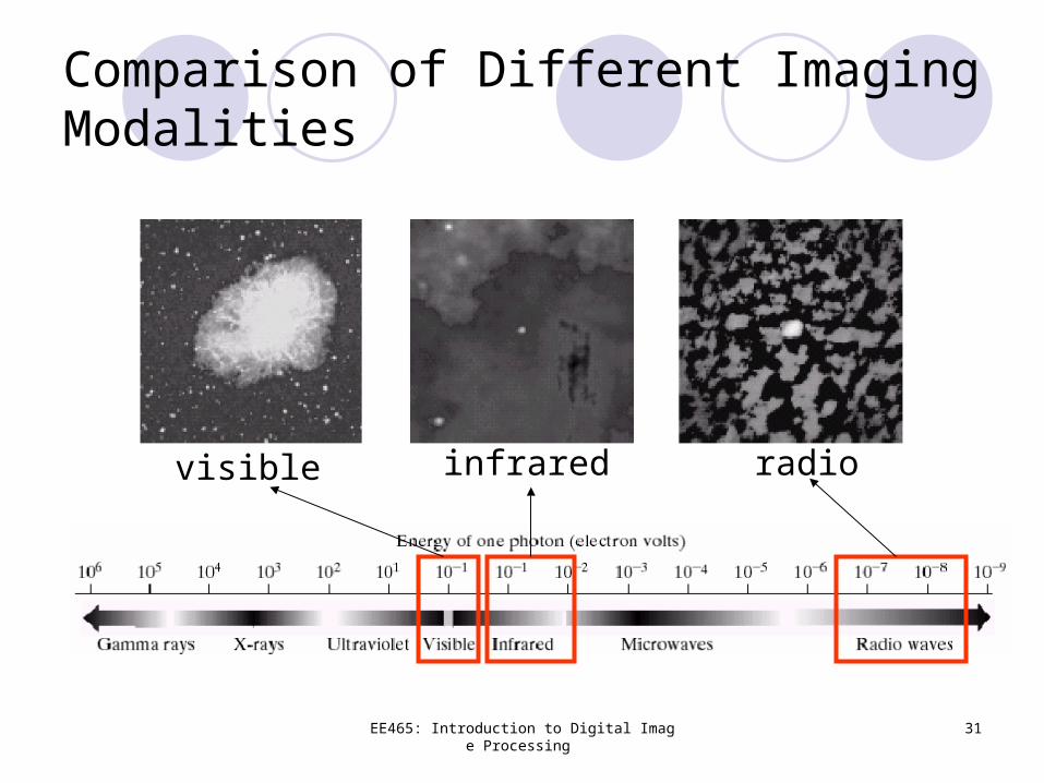
visible infrared radio
Comparison of Different Imaging Modalities
Page 32
EE465: Introduction to Digital Image Processing 32
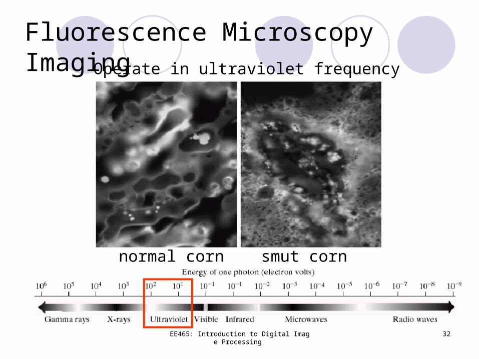
Fluorescence Microscopy Imaging
normal corn smut corn
Operate in ultraviolet frequency
Page 33
EE465: Introduction to Digital Image Processing 33
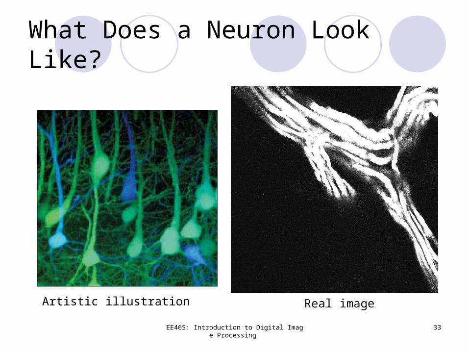
What Does a Neuron Look Like?
Real imageArtistic illustration
Page 34
EE465: Introduction to Digital Image Processing 34
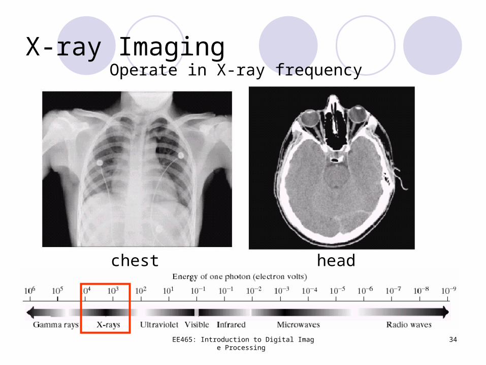
X-ray Imaging
chest head
Operate in X-ray frequency
Page 35
EE465: Introduction to Digital Image Processing 35
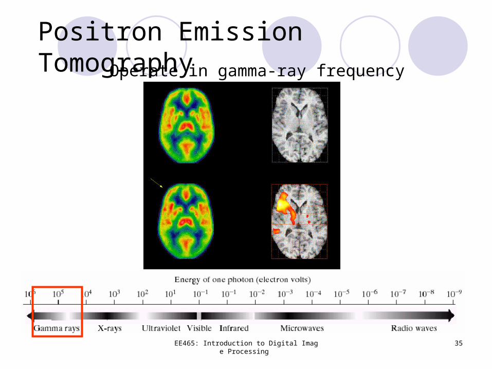
Positron Emission TomographyOperate in gamma-ray frequency
Page 36
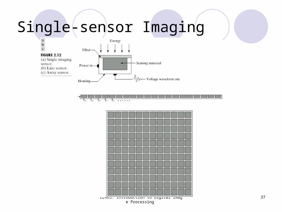
Mechanical Categorization of SensorsMotionless imaging
Sensor is kept still during the acquisition (e.g., CCD cameras)
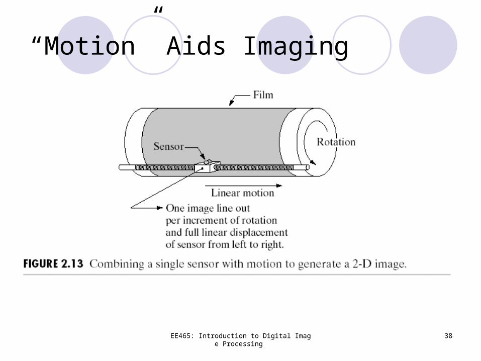
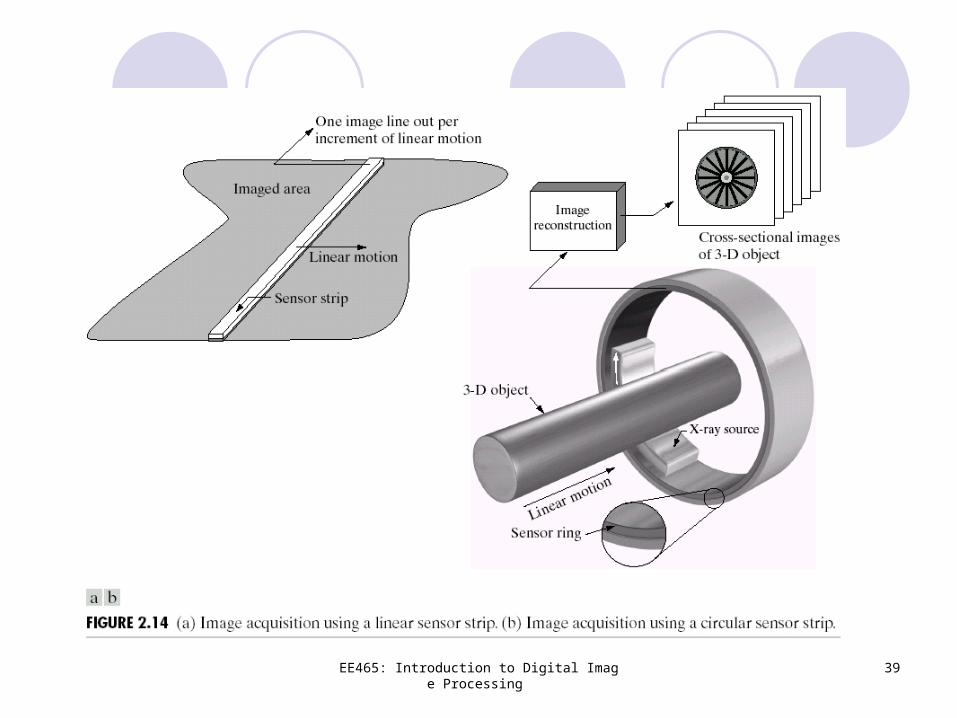
Motion-aided imagingSensor moves along a line or rotates around a center
during the acquisition (e.g., document scanning and MRI scanning)
Subtle relationship between visual perception and motion“We move because we see; we see because we
move” – J. Gibson
EE465: Introduction to Digital Image Processing 36
Page 37
EE465: Introduction to Digital Image Processing 37
Single-sensor Imaging
Page 38
EE465: Introduction to Digital Image Processing 38
“Motion” Aids Imaging
Page 39
EE465: Introduction to Digital Image Processing 39
Page 40
EE465: Introduction to Digital Image Processing 40
Introduction to Grayscale ImagesImage acquisition
Light and Electromagnetic spectrumCharge-Coupled Device (CCD) imagingSampling and Quantization
Image representationSpatial resolutionBit-depth resolutionLocal neighborhoodBlock decomposition
Page 41
EE465: Introduction to Digital Image Processing 41
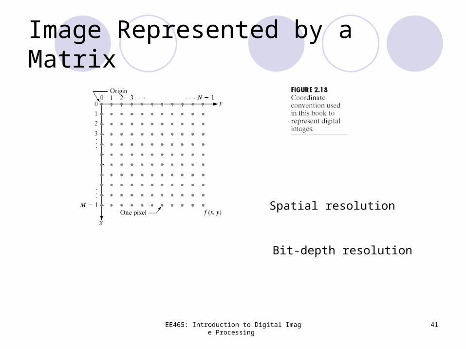
Image Represented by a Matrix
Spatial resolution
Bit-depth resolution
Page 42
EE465: Introduction to Digital Image Processing 42
Spatial Resolution
Page 43
EE465: Introduction to Digital Image Processing 43
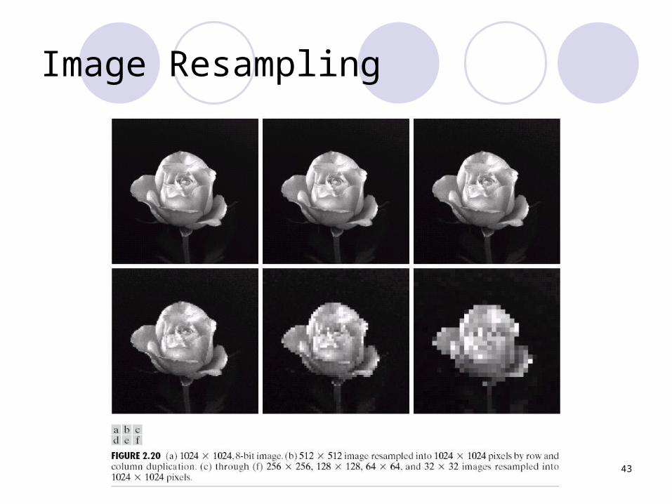
Image Resampling
Page 44
EE465: Introduction to Digital Image Processing 44
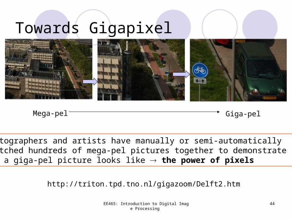
Towards Gigapixel
Mega-pel Giga-pel
http://triton.tpd.tno.nl/gigazoom/Delft2.htm
Photographers and artists have manually or semi-automatically stitched hundreds of mega-pel pictures together to demonstrate how a giga-pel picture looks like the power of pixels
Page 45
EE465: Introduction to Digital Image Processing 45
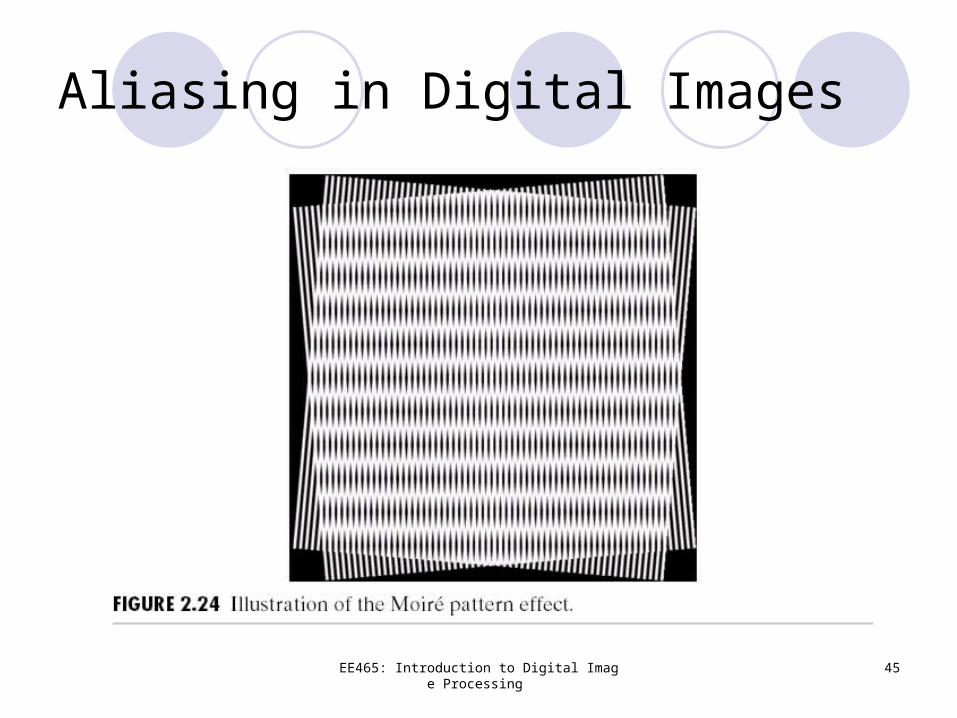
Aliasing in Digital Images
Page 46
EE465: Introduction to Digital Image Processing 46
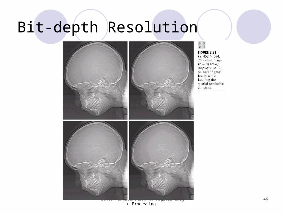
Bit-depth Resolution
Page 47
EE465: Introduction to Digital Image Processing 47
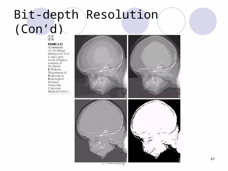
Bit-depth Resolution (Con’d)
Page 48
EE465: Introduction to Digital Image Processing 48
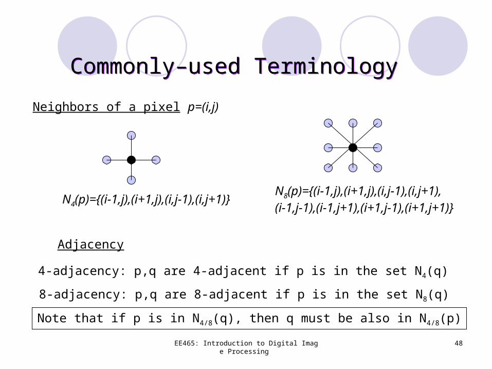
Commonly–used TerminologyCommonly–used Terminology
Neighbors of a pixel p=(i,j)
N4(p)={(i-1,j),(i+1,j),(i,j-1),(i,j+1)}N8(p)={(i-1,j),(i+1,j),(i,j-1),(i,j+1),(i-1,j-1),(i-1,j+1),(i+1,j-1),(i+1,j+1)}
Adjacency
4-adjacency: p,q are 4-adjacent if p is in the set N4(q)
8-adjacency: p,q are 8-adjacent if p is in the set N8(q)
Note that if p is in N4/8(q), then q must be also in N4/8(p)
Page 49
EE465: Introduction to Digital Image Processing 49
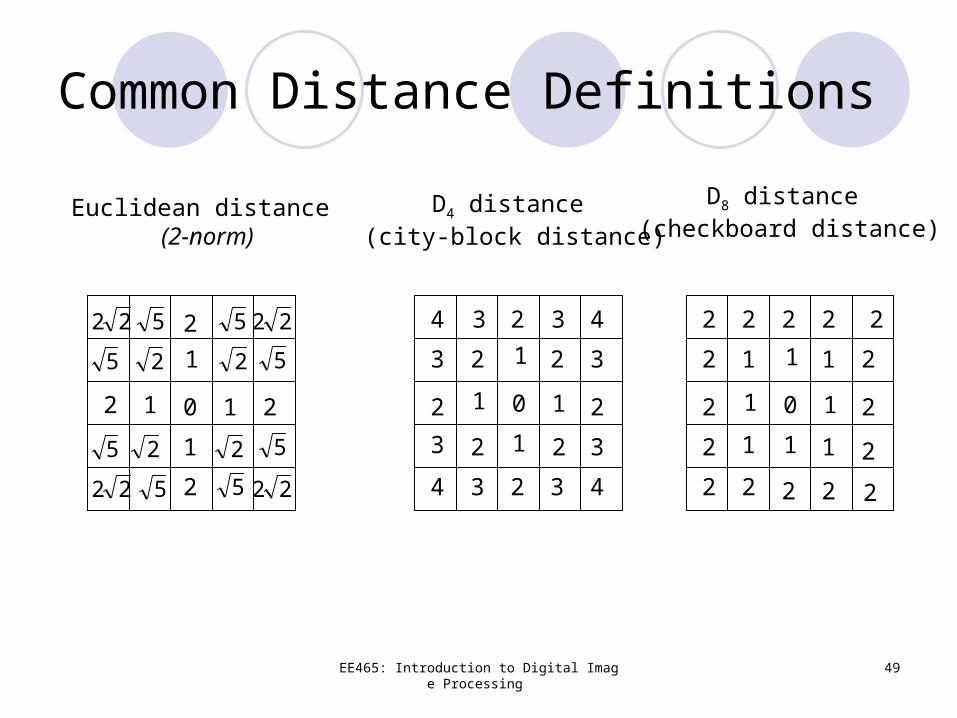
Euclidean distance (2-norm)
D4 distance (city-block distance)
D8 distance (checkboard distance)
01 1
1
1
01 1
1
1
01 1
1
11 1
1 1
2 2 2 2 2
2
2
2
2 2 2 2
2
2
2
2
2
2
2
2
2
2
2
23
3
3
3 3
3
3
34
4 4
42
2 2
2
2 2
22
22
22 22
22
5
5
55
5
5
5 5
Common Distance Definitions
Page 50
EE465: Introduction to Digital Image Processing 50
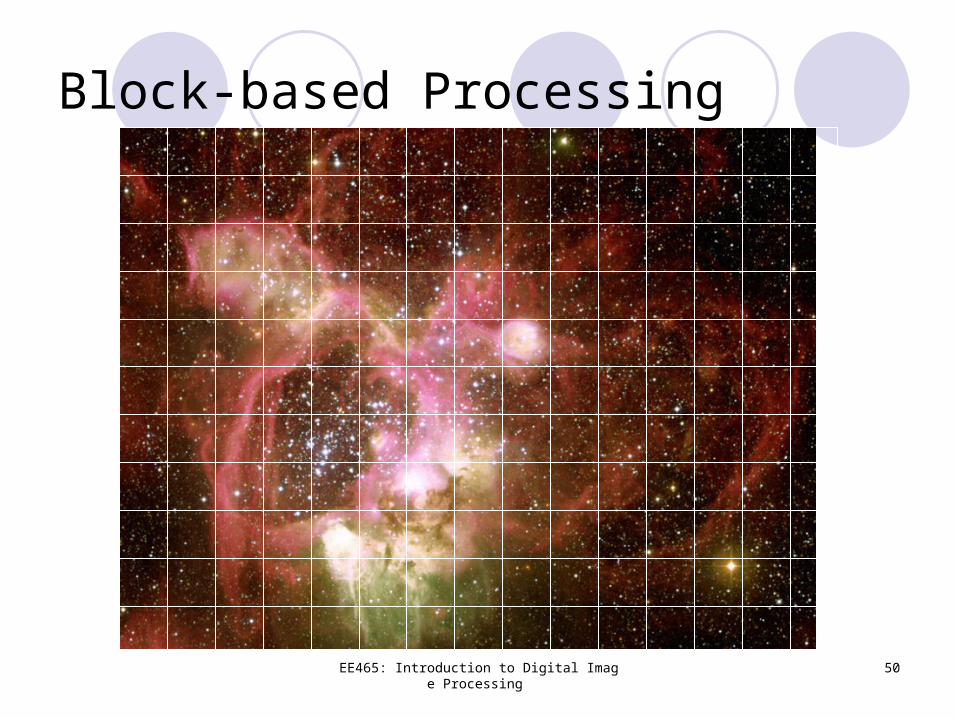
Block-based Processing