22
CASE WESTERN RESERVE UNIVERSITY Discrete and Continuous Time Signals Lab 1 Jared Bell 1/22/2012
| Date post: | 14-May-2017 |
| Category: |
Documents |
| Upload: | josh-immerman |
| View: | 232 times |
| Download: | 0 times |

Case Western Reserve University
Discrete and Continuous Time Signals
Lab 1
Jared Bell
1/22/2012

2.3.1 Analytical Calculation
1.
∫0
2π
sin2 (5t ) dt
∫0
2π 12
(1−cos (2∗5 t ))dt
12∫02π
1dt−¿ 12∫02π
cos (10 t ) dt ¿
12t ¿02 π−
12∗1
10(sin (10 t ) ¿0
2π)
( 2π2 −12∗0)− 1
20(sin (10∗2π )−sin (10∗0 ))
( 2π2 −0)− 120
(0−0)
∫0
2π
sin2 (5t )dt=π
2.
∫0
1
etdt
∫0
1 ddte t dt
e t ¿01
e1−e0
e−1
∫0
1
etdt=e−1=1.718

2.3.2 Displaying Continuous-Time and Discrete-Time Signals in Matlab
The stem plot uses evenly spaced integers between 0 and 60 to show the discrete time
version of the function sin(n/6). The plot of the continuous time function shows the same
function, except in continuous time. These are both accurate graphs. However, the third graph
shows the continuous time function with the integers spaced by 10. As a result this graph
shows undersampling, and is not an accurate representation of the function.
2.3.3 Numerical Computation of Continuous-Time Signals
As the value of N approached 100, the Riemann sum stabilized to a value similar to the
one calculated in the Analytical Calculations. That is for the function sin(5t)2 it approached π,
and for the function e(t) it approached e – 1, or 1.72. The only unusual behavior in the
Riemann sum function were the two spots in the Riemann sum of the sin function graph, where
the sum was approximately 0. I’m assuming that this is due to the rectangles being too large to
accurately approximate the integral. I believe that this is why I(5) = I(10) = 0, however on my

graph it appears to be slightly shifted. When N = 5 in my code, f(t) alternates perfectly between
0 and 1, and the same when N = 10. When N = 6 is when f(t) becomes very small, which is why
when it is multiplied by delta x it approaches 0.
2.4 Processing of Speech Signals

2.5 Attributes of Continuous-Time Signals
Min = -0.1918
Max = 1
Energy = 2.0658
I chose to start at one and go to 100, as it was a broad range that allowed me to see the
signal very easily. However, the graph can probably be truncated at around 50-60, as that is the
point where the signal becomes a shallow sinusoidal centered around 0. So the approximate
start and stop values should be 1 and 60, but I chose 100 for the visual representation of said
sinusoid.

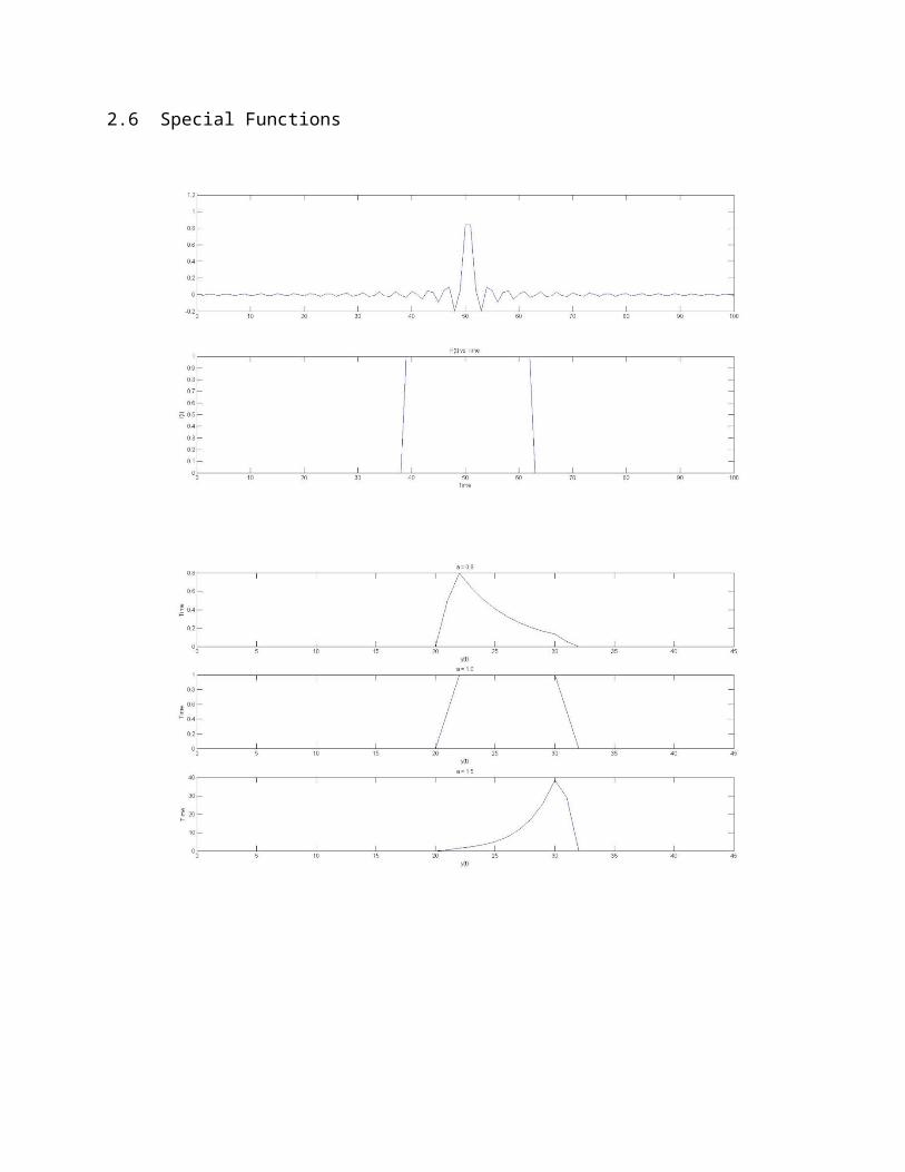
2.6 Special Functions
2.7 Sampling
Changing the sample time lost the information of the sine wave. With Ts = 1/3 the sine
wave became similar to a triangle wave. With Ts = 1/2 it became a line. These first two changes
in the sampling time demonstrate undersampling. With Ts = 10/9, it became just one peak of
the sine wave. The graph was slightly oversampled, but that is hard to tell due to the
constraints of the axes.

2.8 Random Signals
As the value of n increased, the average values settled to their mean values. Essentially
with the increase in n, the average value was statistically more like to be the mean since it is a
Gaussian distribution. This allows the viewer to easily tell the difference between two different
random signals depending on their means.

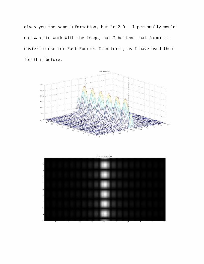
2.9 2-D Signals
The surface plot is visually more appealing to me, as it allows you to visualize and work
in 2-D space easier. The image gives you the same information, but in 2-D. I personally would
not want to work with the image, but I believe that format is easier to use for Fast Fourier
Transforms, as I have used them for that before.

Appendix: Code
Main
%% Header % Jared Bell% EECS 313% Lab 1 - Discrete and Continuous Time Signals% 1/22/12 %% 2.3.2 Displaying Continuous Time and Discrete Time Signals in Matlab % This section establishes n as a series of evenly spaced integers (by 2)% between 0 and 60, then plots them according the the y function.n = 0:2:60;y = sin(n/6);subplot(3,1,1)stem(n,y)title('Discrete Time');xlabel('Time');ylabel('y(n)'); % This section does the same as the previous section, however it uses plot% instead of stem, to be used similar to a continuous time function. This% is an accurate extrapolation of the data.n1 = 0:2:60;z = sin(n1/6);subplot(3,1,2)plot(n1,z)title('Continuous Time');xlabel('Time');ylabel('y(n)'); % This section does the same as the previous, however it shows% undersampling due to the integer points being spaced by 10. As a result,% this is a very inaccurate graph of the sin function.n2 = 0:10:60;w = sin(n2/6);subplot(3,1,3)plot(n2,w)title('Continuous Time Undersampled');xlabel('Time');ylabel('y(n)'); pause %% 2.3.3 Numerical Computation of Continuous-Time Signals % functions are called to calculate riemann sum based off of N I = 1:100; % presetting vector length to save memory

J = 1:100; for Ncounter = 1:100 I(Ncounter) = integ1(Ncounter); J(Ncounter) = integ2(Ncounter); % calling htem both to save for loops end subplot(2,1,1)plot(I)xlabel('N rectangles');ylabel('Area');title('Riemann sum of sin(5t)^2'); subplot(2,1,2)plot(J)xlabel('N rectangles');ylabel('Area');title('Riemann sum of exp(t)'); % Note that as N approaches 100 the value of the area becomes approximately% the value solved for in the analytical solutions, that is pi and e - 1% (1.72). pause %% 2.4 Processing of Speech Signals audio_vector = auread('speech.au'); % loads the speech filefigure;plot(audio_vector);title('Speech.au File'); % plotted and labeled sound(audio_vector); % this plays the file pause %% 2.5 Attributes of Continuous-Time Signals t = 0:100;plot(signal1(t)); % Every integertitle('Signal1(t)');xlabel('Time');ylabel('y(t)'); pause t2 = 0:2:100;plot(signal1(t2)); % Every other integer t3 = 0:2:50;plot(signal1(t3)); % Every other integer to 50

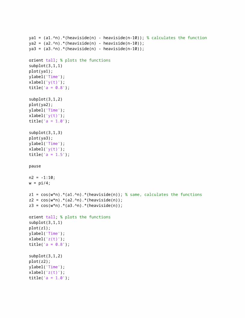
minSignal = minSignal1(t); % calls functions to return min and max valuesmaxSignal = maxSignal1(t);energySignal = energySignal1(t); pause %% 2.6 Special Functions t_sinc = linspace(-10*pi,10*pi);t_rect = linspace(-2,2); y = sinc(t_sinc);z = (abs(t_rect)<=0.5); subplot(2,1,1)plot(y);subplot(2,1,2)plot(z);xlabel('Time');ylabel('f(t)');title('F(t) vs Time'); pause a1 = 0.8;a2 = 1.0;a3 = 1.5; n = -20:20; ya1 = (a1.^n).*(heaviside(n) - heaviside(n-10)); % calculates the functionya2 = (a2.^n).*(heaviside(n) - heaviside(n-10));ya3 = (a3.^n).*(heaviside(n) - heaviside(n-10)); orient tall; % plots the functionssubplot(3,1,1)plot(ya1);ylabel('Time');xlabel('y(t)');title('a = 0.8'); subplot(3,1,2)plot(ya2);ylabel('Time');xlabel('y(t)');title('a = 1.0'); subplot(3,1,3)plot(ya3);ylabel('Time');xlabel('y(t)');title('a = 1.5');

pause n2 = -1:10;w = pi/4; z1 = cos(w*n).*(a1.^n).*(heaviside(n)); % same, calculates the functionsz2 = cos(w*n).*(a2.^n).*(heaviside(n));z3 = cos(w*n).*(a3.^n).*(heaviside(n)); orient tall; % plots the functionssubplot(3,1,1)plot(z1);ylabel('Time');xlabel('z(t)');title('a = 0.8'); subplot(3,1,2)plot(z2);ylabel('Time');xlabel('z(t)');title('a = 1.0'); subplot(3,1,3)plot(z3);ylabel('Time');xlabel('z(t)');title('a = 1.5'); pause %% 2.7 Sampling Ts1 = 1/10; % establishes constantsTs2 = 1/3;Ts3 = 1/2;Ts4 = 10/9; ns1 = 0:100;ns2 = 0:30;ns3 = 0:20;ns4 = 0:9; xn1 = sin(2*pi*Ts1*ns1); % calculates functionsxn2 = sin(2*pi*Ts2*ns2);xn3 = sin(2*pi*Ts3*ns3);xn4 = sin(2*pi*Ts4*ns4); subplot(4,1,1)plot(xn1)ylabel('Time');xlabel('x(n)');title('Ts = 1/10');axis([0,100,-1,1]);

subplot(4,1,2)plot(xn2)ylabel('Time');xlabel('x(n)');title('Ts = 1/3');axis([0,30,-1,1]); subplot(4,1,3)plot(xn3)ylabel('Time');xlabel('x(n)');title('Ts = 1/2');axis([0,20,-1,1]); subplot(4,1,4)plot(xn1)ylabel('Time');xlabel('x(n)');title('Ts = 10/9');axis([0,9,-1,1]); % Changing the sample time lost the information of the sine wave. With Ts% = 1/3 the sine wave became similar to a triangle wave. With it equal to% 1/2 it became a line. With it equal to 10/9, it became just one peak of% the sine wave. pause %% 2.8 Random Signals sig1 = random('norm',0,1,1000);sig2 = random('norm',0.2,1,1000); % random signals subplot(2,1,1)plot(sig1)title('Signal 1 Mean=0 Variance=1');subplot(2,1,2)plot(sig2)title('Signal 2 Mean=0.2 Variance=1'); pause ave1 = 1:1000;ave2 = 1:1000; for counter = 1:1000 % use a for loop to make a summation of the averages ave1(counter) = mean(sig1(1:counter)); ave2(counter) = mean(sig2(1:counter)); end figure;plot(ave1, 'k');
hold onplot(ave2, 'b');title('Average of the Random Signals Based on n');xlabel('n');ylabel('Average');legend('Average1', 'Average2');hold off pause %% 2.9 2-D Signals m = linspace(-50,50);n = linspace(-50,50); [x,y] = meshgrid(m,n); % generates arrays f = 255.*(abs(sinc(0.2.*x).*sin(0.2.*y))); % calculates function mesh(f); % mesh plot to display the signaltitle('Mesh plot of f(m,n)');pause image(f); % make imagetitle('Grayscale image of f(m,n)');colormap(gray(256)); % grayscale
Integ1
function [ I ] = integ1( N )%INTEG1 does a reimann sum approximation based off the number of rectangles%N t = linspace(0,2*pi,N); % makes evenly spaced based off number of rectangles delta = t(end)/N; ft = sin(5.*t).^2; % calculates height A = ft.*delta; % calculates area I = sum(A); % sums end
Integ2
function [ J ] = integ2( N )

%INTEG2 Riemann sum calculation based of the number of rectangles N t = linspace(0,1,N); % makes evenly spaced based off number of rectangles delta = t(end)/N; ft = exp(t); % calculates height A = ft.*delta; % calculates area J = sum(A); % sums end
MinSignalfunction [ minSignal ] = minSignal1(t)%MINSIGNAL1 - Calculates the minimum of a signal over a range of time% Takes input arguement and calculates the minimum, calls signal1 minSignal = min(signal1(t)); end
MaxSignalfunction [ maxSignal ] = maxSignal1(t)%MAXSIGNAL1 - Calculates the maximum of a signal over a range of time% Takes input arguement and calculates the maximum, calls signal1 maxSignal = max(signal1(t)); end
EnergySignalfunction [ energySignal ] = energySignal1(t)%ENERGYSIGNAL1 - Calculates the energy of a signal over a range of time% Takes input arguement and calculates the energy by intergrating and% calling signal1 absSignal = abs(signal1(t)); % This takes care of the absolute valuesignalSquared = absSignal.^2; % takes care of the squaringenergySignal = sum(signalSquared); % summation of the data end


