Page 1
EECS487:Interactive
ComputerGraphicsLecture37:• B-splinescurves• RationalBézierandNURBS
CubicSplinesArepresentationofcubicsplineconsistsof:
• fourcontrolpoints(whyfour?)• thesearecompletelyuserspecified
• determineasetofblendingfunctions
Thereisnosingle“best”representationofcubicspline:
*n/awhensomeofthecontrol“points”aretangents,notpoints
Cubic Interpolate? Local? Continuity Affine? Convex*? VD*?
Hermite � � C1 � n/a n/a
Cardinal
(Catmull-Rom)
except
endpoints
� C1 � no no
Bézier endpoints � C1 � � �
natural � � C2 � n/a n/a
B-splines � � C2 � � �
NaturalCubicSplineAnaturalcubicspline’scontrolpoints:
• positionofstartpoint• 1stderivativeofstartpoint
• 2ndderivativeofstartpoint
• positionofendpoint
• constraintandbasismatrices:
• subsequentsegmentsassumethepositionand1stand2nd
derivativesoftheendpointoftheprecedingsegment
C =
1 0 0 00 1 0 00 0 2 01 1 1 1
⎡
⎣
⎢⎢⎢⎢
⎤
⎦
⎥⎥⎥⎥
, B = C−1 =
1 0 0 00 1 0 00 0 1
2 0−1 −1 − 1
2 1
⎡
⎣
⎢⎢⎢⎢
⎤
⎦
⎥⎥⎥⎥
f (u) = a0 + u1a1 + u2a2 + u3a3
p0 = f (0) = a0 + 01a1 + 02 a2 + 03a3
p1 = f '(0) = a1 + 2*01a2 + 3*0
2 a3p2 = f ''(0) = 2*11a2 + 6*0
2 a3p3 = f (1) = a0 + 11a1 + 12 a2 + 13a3
NaturalCubicSpline
Givenncontrolpoints,anaturalcubicsplinehasn−1 segments
Forsegmenti:
Set:
O’Brien
fi (0) = pi−1, i = 1,…,nfi (1) = pi , i = 1,…,n
fi' (0) = fi−1
' (1), i = 1,…,n −1fi"(0) = fi−1
" (1), i = 1,…,n −1
f1"(0) = fn
"(1) = 0
Page 2
NaturalCubicSplines
Eachcurvesegment(otherthanthefirst)receives
threeoutofitsfourcontrolpointsfromthe
precedingsegment,thisgivesthecurveC2continuity
Howeverthepolynomialcoefficientsare
dependentonallncontrolpoints• controlisnotlocal:anychangeinanysegment
maychangethewholecurve
• curvetendstobeill-conditioned:asmallchange
atthebeginningcanleadtolargesubsequentchanges
B-splines
TP3,Watt
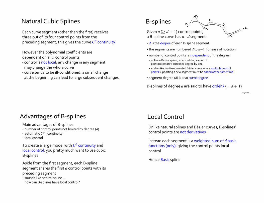
Givenn(≥ d + 1)controlpoints,aB-splinecurvehasn−dsegments
• disthedegreeofeachB-splinesegment
• thesegmentsarenumbereddton−1,foreaseofnotation• numberofcontrolpointsisindependentofthedegree
• unlikeaBézierspline,whereaddingacontrol
pointnecessarilyincreasesdegreebyone,
• andunlikemulti-segmentedBéziercurvewheremultiplecontrol
pointssupportinganewsegmentmustbeaddedatthesametime
• segmentdegree(d)isalsocurvedegree
B-splinesofdegreedaresaidtohaveorderk(= d + 1)
AdvantagesofB-splinesMainadvantagesofB-splines:• numberofcontrolpointsnotlimitedbydegree(d)• automaticCd�1continuity
• localcontrol
TocreatealargemodelwithC2continuityand
localcontrol,youprettymuchwanttousecubic
B-splines
Asidefromthefirstsegment,eachB-spline
segmentsharesthefirstdcontrolpointswithits
precedingsegment• soundslikenaturalspline…
howcanB-splineshavelocalcontrol?
LocalControl
UnlikenaturalsplinesandBéziercurves,B-splines’
controlpointsarenotderivatives
Insteadeachsegmentisaweighted-sumofdbasisfunctions(only),givingthecontrolpointslocal
control
HenceBasisspline
Page 3
WhyisBcalledtheBasisMatrix?
PolynomialsasaVectorSpace
Polynomialsf (u) = a0 + a1u + a2u2 + … + anun
• canbeadded:justaddthecoefficients
• canbemultipliedbyascalar:multiplythecoefficients
• areclosedunderadditionandmultiplicationbyscalar
• i.e.,theresultisstillapolynomial
�It’savectorspace!
Avectorspaceisdefinedbyasetofbasis
• linearlyindependentvectors• linearcombinationofthebasisvectorsspansthespace
• herevector=polynomial
Durand
CanonicalPowerBasis1, u, u2, u3, … , un
• areindependent• anypolynomialisalinearcombinationofthese,
a0 + a1u + a2u2 + … + anun
• oftencalledthecanonicalbasisfunctions
JustaswithEuclideanspace,
thereareinfinitenumberofpossiblebasis
Forcubic,thebasisfunctionscouldbe,forexample:
• 1, 1+u, 1+u+u2, 1+u–u2+u3
• u3, u3–u2, u3+u, u3+1
Durand
BasisMatrixandBasisFunctions
Abasismatrix(B)transformsthecanonicalbasis(u)toanotherbasis:
Thebi(u)’sarethebasisfunctionsoftheotherbasis(we’veknownthemastheblendingfunctions)
f (u) = ua = uBp = (1− u)p0 + up1 = bi (u)pii=0
n
∑
uB = bi (u)i=0
n
∑
Page 4
B-splines
Givenncontrolpoints,therearen−dsegments
• wecallthesegmentsfi(u),d ≤ i < n• eachsegmenthasaunitrange,0 ≤ u ≤1
• wecalltheentireB-splinecurvewithncontrolpointsf(t)
Theparametersti’swheretwosegmentsjoinare
calledknots
• thestartandendpoints(tdandtn)
arealsocalledknots
• therange[td, tn]isthedomain
ofaB-splinecurve
• theparameteruofsegmentiisscaledtoti ≤ u < ti+1
y(t) P9
P3
P1
P8
P4
P7
P6
P5
P2
P0
Q9
Q8
Q7
Q6
Q5
Q4
Q3
t3
t5
t6
t7
t4
t8
t9
t10
Knot
Control pointx(t)
Foley,vanDam90
f3(u)f4(u)
f5(u)
f6(u)
f7(u)
f8(u)
f9(u)
acubicB-spline
UniformB-splines
TheknotsofauniformB-splinesarespacedat
equalintervals
y(t) P9
P3
P1
P8
P4
P7
P6
P5
P2
P0
Q9
Q8
Q7
Q6
Q5
Q4
Q3
t3
t5
t6
t7
t4
t8
t9
t10
Knot
Control pointx(t)
f3(u)f4(u)
f5(u)
f6(u)
f7(u)
f8(u)
f9(u)
acubic
B-spline
Foley,vanDam90
Arbitrarycurveshaveanuncountablenumberofparameters
Real-numberfunctionvalueexpandedintoaninfinitesetofbasisfunctions:
Approximatebytruncatingsetatsomereasonablepoint,e.g.,3:
WhatDegreeisSufficient?
O’Brien
f (u) = bi (u)pii=0
∞
∑
f (u) = bi (u)pii=0
3
∑
Inthelinearcase,thebasisfunctionsare
b0(u) = (1−u)andb1(u) = u
(a.k.a.tent/trianglebasis,thei’thfunctionsareshiftedversionsofthe0’th)
LinearB-splineSegment
0 1 2
1
James,Hanrahan
b(u) =
0 u < −11+ u −1< u < 01− u 0 < u <10 u >1
⎧
⎨⎪⎪
⎩⎪⎪
⎫
⎬⎪⎪
⎭⎪⎪
Page 5
LinearB-splineCurve
ConsiderusinglinearB-splines(d=1,k=2)todraw
apiecewiselinearcurve(apolyline)
Todrawthecurve,weperformlinearinterpolation
ofasetofcontrolpointsp0, …, pn–1
Forsegmenti,wewritetheinterpolatinglinear
curveasfi(u) = (1−u)pi–1+ upi,where u =t − titi+1 − ti
∈ 0,1[ ]
p0 pn–1 pi–2
pi–1 pi+1 pi+2
pi
t = i–1
t = i
t = i+1
t = i+2
t = i+3
fi(u)
[Craig]
LinearB-splines
Theinfluenceofcontrolpointpionthewholecurve
isthusthe“tent/triangle”function:
ThehardestpartofworkingwithB-splinesis
keepingtrackofthetediousnotations!
[Craig]
ti ti+1 ti+2
bi(t)1
bi (t) =
t − titi+1 − ti
, ti ≤ t < ti+1,
ti+2 − tti+2 − ti+1
, ti+1 ≤ t < ti+2 ,
0, everywhereelse
⎧
⎨
⎪⎪⎪
⎩
⎪⎪⎪
t − titi+1 − ti
ti+2 − tti+2 − ti+1
pi−1pi
pi+1
LinearB-splines
Linearlyinterpolatingthesetofcontrolpointstodraw
thecurve:
fi (u) = (1− u)pi−1 + upi =ti+1 − tti+1 − ti
pi−1 +t − titi+1 − ti
pi , u =t − titi+1 − ti
, ti ≤ t < ti+1
fi+1(u) = (1− u)pi + upi+1 =ti+2 − tti+2 − ti+1
pi +t − ti+1ti+2 − ti+1
pi+1, u =t − ti+1ti+2 − ti+1
, ti+1 ≤ t < ti+2
[Craig]
ti–1 ti ti+1 ti+2 ti+3
f(t) upi+1upi
(1�u) pi(1�u) pi−1
pipi−1p0
pi+1pi−2 pn−1
pi+2
fi(u)
fi+1(u)
LinearB-splines
Wecanrewritethesegmentfunctionsas:
Andforthewholecurve:
wherebi(t)’sarethebasisfunctions(inthiscase,linear)
fi (t) = bi−1(t)pi−1 + bi (t)pi , ti ≤ t < ti+1fi+1(t) = bi (t)pi + bi+1(t)pi+1, ti+1 ≤ t < ti+2
[Craig]
f (t) = fi (t) = bi (t)pii=1
n−1
∑i=1
n−1
∑
fi (u) = (1− u)pi−1 + upi =ti+1 − tti+1 − ti
pi−1 +t − titi+1 − ti
pi , u =t − titi+1 − ti
, ti ≤ t < ti+1
fi+1(u) = (1− u)pi + upi+1 =ti+2 − tti+2 − ti+1
pi +t − ti+1ti+2 − ti+1
pi+1, u =t − ti+1ti+2 − ti+1
, ti+1 ≤ t < ti+2
Page 6
QuadraticB-splinesQuadraticB-splines(d=2,k=3)aredrawnbytwo
interpolationsteps,similarbutdifferenttoquadratic
Bézier
WhereasdeCasteljaualgorithmperformstheiterative
interpolationsforBéziercurves,deBooralgorithm
doessoforB-splines[TP3,Buss]
4/5
1/5 4/5
1/5 1/5
4/5
Bézierquadratic:
parameter“along”edge
B-splinesquadratic:
parameter“around”
controlpoint
pi–2
pi–1
pi
qi–1
qi
f(t)
deBoorAlgorithmDeBooralgorithmisaniterativeinterpolation
algorithmthatgeneralizesdeCasteljau’salgorithm
ToevaluateaB-splinecurvef(t) atparametervaluet:1. determinethe[ti, ti+1)inwhichtbelongs;
d ≤ i < n,thedomainofthecurveis[td, tn]2. tocomputef(t)ofdegreed,firstinterpolatebetween
controlpointsp’s3. then,inabottomupfashion,continuetoperformrroundsofpairwiselinearinterpolations,untilr = d,using:
[TP3,Buss]
f j ,dr (t) =
t j+k−r − tt j+k−r − t j
f j−1r−1(t)+
t − t jt j+k−r − t j
f jr−1(t),
t j ≤ t < t j+k−r ,1≤ r ≤ d,
j = i − d + r, i − d + r +1, …,i
QuadraticB-splines
UsingthedeBooralgorithmwefirstcomputeqi–1
andqi(note:overtwoknotintervals):
[TP3,Buss]
B-splinesquadratic
pi–2
pi–1
pi
qi–1
qi
f(t)
qi−1 = fi−1,21 (t) = ti+1 − t
ti+1 − ti−1pi−2 +
t − ti−1ti+1 − ti−1
pi−1, ti−1 ≤ t < ti+1
qi = fi,21 (t) = ti+2 − t
ti+2 − tipi−1 +
t − titi+2 − ti
pi , ti ≤ t < ti+2
QuadraticB-splines
Thenwelinearlyinterpolatebetweenqi–1andqiin
asecondround(r = 2)ofinterpolation:
[TP3,Buss]
B-splinesquadratic
pi–2
pi–1
pi
qi–1
qi
f(t)
fi,22 (t) = ti+1 − t
ti+1 − tiqi−1 +
t − titi+1 − ti
qi , ti ≤ t < ti+1
f (t) = ti+1 − tti+1 − ti
ti+1 − tti+1 − ti−1
pi−2
+ ti+1 − tti+1 − ti
t − ti−1ti+1 − ti−1
+ t − titi+1 − ti
ti+2 − tti+2 − ti
⎛⎝⎜
⎞⎠⎟pi−1
+ t − titi+1 − ti
t − titi+2 − ti
pi
Page 7
QuadraticB-splines
Thecontrolpointpiinfluencesfi,2(t),fi+1,2(t),andfi+2,2(t),fromwhichwecanassembleitsblending
function:
[TP3,Buss]
!
bi (t) =
ti+1 − tti+1 − ti
ti+1 − tti+1 − ti−1
, ti ≤ t < ti+1,
ti+1 − tti+1 − ti
t − ti−1ti+1 − ti−1
+ t − titi+1 − ti
ti+2 − tti+2 − ti
, ti+1 ≤ t < ti+2 ,
t − titi+1 − ti
t − titi+2 − ti
, ti+2 ≤ t < ti+3,
0, everywhere!else
⎧
⎨
⎪⎪⎪⎪
⎩
⎪⎪⎪⎪
fi(t)fi+1(t)
fi+2(t) InterpolationandBasisFunctions
Bézier B-splineinterpolation deCasteljau deBoor
basisfunctionsBernstein
polynomials
Cox-deBoor
recurrence
Cox-deBoorRecurrencedeBooralgorithmconstructsbasisfunctions“bottom-
up”,whereasCox-deBoorrecurrencegeneratesthe
basisfunctions“top-down”
Letbi,k(t)beak-thorderbasisfunctionforweighting
controlpointpi,• ifthedenominatoris0(non-uniformknots),
thebasisfunctionisdefinedtobe0• Cox-deBoorrecurrenceessentiallytakesalinearinterpolationoflinearinterpolationsoflinearinterpolations,similartothedeCasteljaualgorithm
bi,1(t) =1, ti ≤ t < ti+1 (both ≤ forlastsegment),0, otherwise
⎧⎨⎪
⎩⎪
bi,k (t) =t − ti
ti+k−1 − tibi,k−1(t)+
ti+k − tti+k − ti+1
bi+1,k−1(t)
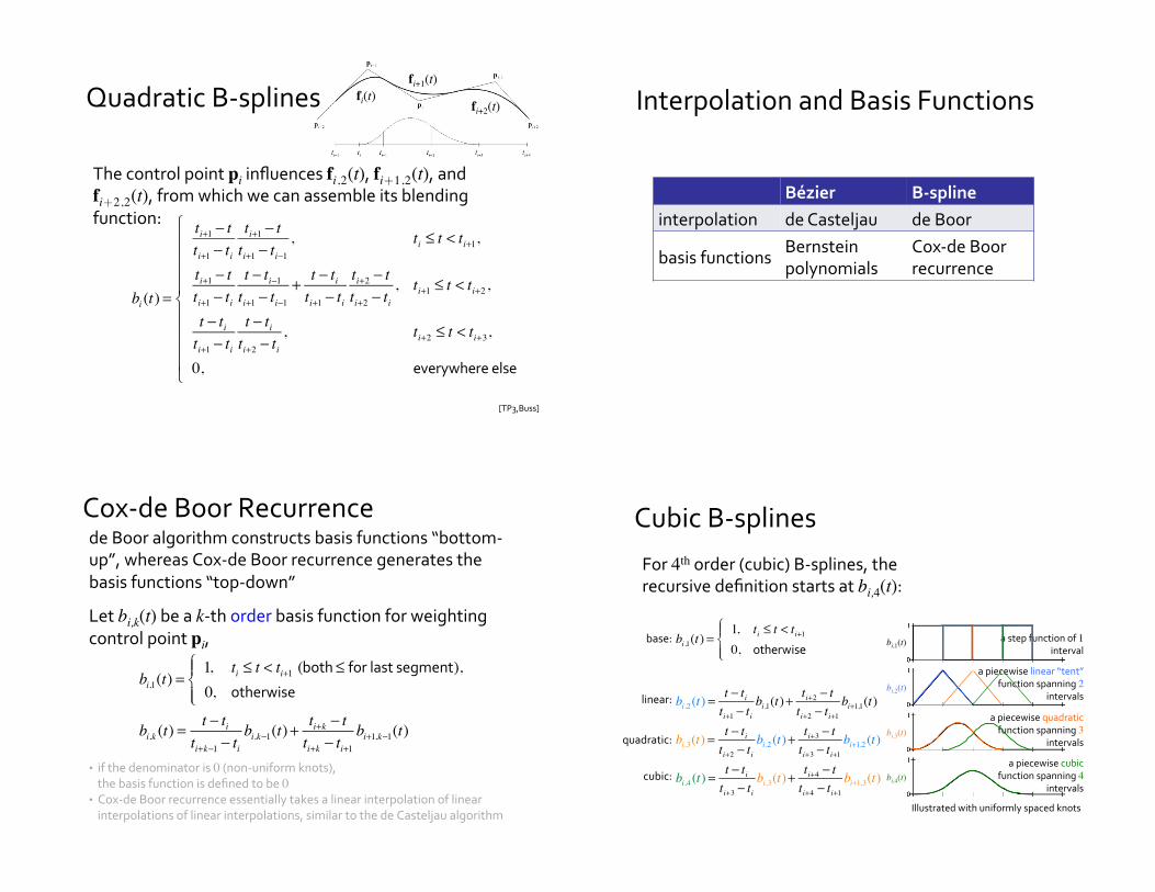
CubicB-splines
For4thorder(cubic)B-splines,the
recursivedefinitionstartsatbi,4(t):
base:
linear:
quadratic:
cubic:
astepfunctionof1interval
apiecewiselinear“tent”
functionspanning2intervals
apiecewisequadratic
functionspanning3intervals
apiecewisecubic
functionspanning4intervals
Illustratedwithuniformlyspacedknots
bi,4(t)
bi,1(t)
bi,3(t)
bi,2(t)
bi,1(t) =1, ti ≤ t < ti+10, otherwise
⎧⎨⎪
⎩⎪
bi,2 (t) =t − titi+1 − ti
bi,1(t)+ti+2 − tti+2 − ti+1
bi+1,1(t)
bi,3(t) =t − titi+2 − ti
bi,2 (t)+ti+3 − tti+3 − ti+1
bi+1,2 (t)
bi,4 (t) =t − titi+3 − ti
bi,3(t)+ti+4 − tti+4 − ti+1
bi+1,3(t)
Page 8
UniformCubicBasisFunctionConstructedfromtheCox-deBoorrecurrence• takingadvantageoffixedintervalbetweenknots
• consideringonlyintervalsforwhichthebasisfunction
isnon-zero
�
bi(t)
ti ti+1 ti+2 ti+3 ti+4
[Buss,Shirley,Gleicher]
!
Let!ti = i,!specializing!for!i = 0:
b0,4 (t) = !
t 3
6, 0 ≤ t <1,
−3t 3 +12t 2 −12t + 46
, 1≤ t < 2,
3t 3 − 24t 2 + 60t − 446
, 2 ≤ t < 3,
−t 3 +12t 2 − 48t + 646
, 3≤ t < 4,
0, everywhere!else
⎧
⎨
⎪⎪⎪⎪⎪⎪
⎩
⎪⎪⎪⎪⎪⎪
bi,1(t) =1, ti ≤ t < ti+10, otherwise
⎧⎨⎪
⎩⎪b1,2 (t) = t − ti( )bi,1(t)+ ti+2 − t( )bi+1,1(t)bi,3(t) =
t − ti2
bi,2 (t)+ti+3 − t2
bi+1,2 (t)
bi,4 (t) =t − ti3
bi,3(t)+ti+4 − t3
bi+1,3(t)
y(t)
P3
P1
P8
P4
P7
P6
P5P
2
P0
Q8
Q7
Q6
Q5
Q4
Q3
Knot
Control pointx(t)
P’4
P’’4
P’’4Curve
P’4Curve
CurveP4
LocalControlPropertyForuniform,multi-segmentB-splinecurves,theknotvaluesareequally
spacedandeachbasisfunctionisacopyandtranslateofeachother
WedefinetheentiresetofcurvesegmentsasoneB-splinecurveint:
Thecurveisalinearcombinationofall
thebasisfunctionsofthesegments:
f(t) = bi (t)pi
i=0
n−1
∑ , t ∈[3,n]
domainofcurve
�
b0(t)
�
b1(t)
�
b2(t)
�
b3(t)
�
b4 (t)
�
b5(t)
�
b6(t)
�
b7(t)
�
b8(t)
• eachsegmentisinfluencedbyfour
(non-zero)basisfunctions
• eachcontrolpointisscaledbyasinglebasisfunction
• eachbasisfunctionisnon-zerooverfoursuccessiveintervalsint� eachcontrolpointinfluencesfour
segments(only)�localcontrol
f(t)
BBs—2
t
—66
—56
—46
—36
—26
—16
BBs—1
BBs—3BBs0
0 1
�
bi−3
�
bi
�
bi−2
�
bi−1
t
b(t)
�
b4 (t)
t=i t=i+1 t=i+2 t=i+3 t=i+4
Foley,vanDam90
Watt00
f3(u)f8(u)f4(u)
f5(u)f6(u)
f7(u)
ConvexHullProperty
Thebasisfunctionis≥ 0andsumsto
unityintherangetitoti+4 � allthecontrolpointsformaconvexhull
� thewholecurveiswithintheconvexhull
Betweenknotvalues,thefourbasis
functionsarenon-zeroandsumtounity
Ateachknotvalue,onebasisfunction
“switchesoff”andanother“switcheson”,and
threebasisfunctionsarenon-zeroandsumtounity
domainofcurve
�
b0(t)
�
b1(t)
�
b2(t)
�
b3(t)
�
b4 (t)
�
b5(t)
�
b6(t)
�
b7(t)
�
b8(t)
f(t)
BBs—2
t
—66
—56
—46
—36
—26
—16
BBs—1
BBs—3BBs0
0 1
�
bi−3
�
bi
�
bi−2
�
bi−1
u
b(u)
bi−k (t)k=0
3
∑ = 1, ti ≤ t < ti+1
bi− k(t ) ≥ 0, 3 ≤ i < n, 0 ≤ k ≤ 3
�
bi(t)
ti ti+1 ti+2 ti+3 ti+4
UniformCubicB-spline
SegmentBasisFunctions
BasisfunctionsforasingleB-splinesegment���• shiftedpiecesofasinglebasisfunctiontou∈[0,1]range
Specializingfori = 0:
!
bi,4 (u) =u3
6, u = t, !0 ≤ t <1
bi−1,4 (u) =−3u3 + 3u2 + 3u +1
6, u = t −1, !1≤ t < 2
bi−2,4 (u) =3u3 − 6u2 + 4
6, u = t − 2, !2 ≤ t < 3
bi−3,4 (u) =(1− u)3
6, u = t − 3, !3≤ t < 4
f(t)
BBs—2
t
—66
—56
—46
—36
—26
—16
BBs—1
BBs—3BBs0
0 1
�
bi−3
�
bi
�
bi−2
�
bi−1
u
b(u)
[Shirley,Gleicher]
Page 9
Controlpointsforonesegmentfi(u)arepi-3,pi-2,
pi-1,pi,3 ≤ i < n,recall:thecontrolpointscantakeonarbitraryvalues(geometricconstraints)
Asegmentisdescribedas:
ThecubicB-splinesegment
basismatrixis:
y(t) P9
P3
P1
P8
P4
P7
P6
P5
P2
P0
Q9
Q8
Q7
Q6
Q5
Q4
Q3
t3
t5
t6
t7
t4
t8
t9
t10
Knot
Control pointx(t)
Foley,vanDam90
f3(u)f4(u)
f5(u)
f6(u)
f7(u)
f8(u)
f9(u)
UniformCubicB-splineSegment
fi (u) = bi−3+ j (u)pi−3+ jj=0
3
∑ , u ∈[0,1]
= (1− u)3
6pi−3 +
3u3 − 6u2 + 46
pi−2 +
−3u3 + 3u2 + 3u +16
pi−1 +u3
6pi
B = 16
−1 3 −3 13 −6 3 0−3 0 3 01 4 1 0
⎡
⎣
⎢⎢⎢⎢
⎤
⎦
⎥⎥⎥⎥
BézierisNotB-spline
Relationshiptothecontrolpointsisdifferent
Bézier
B-spline
Durand
Interpolation
AB-splinecurvedoesn’thavetointerpolateany
ofitscontrolpoints
Interpolationwith
MultipleControlPoints
AB-splinecurvecanbemadetointerpolateoneor
moreofitscontrolpointsbyaddingmultiplecontrol
pointsofthesamevalue,atthelossofcontinuity
Examples:
Watt00
C2G2
C2G1 C2G0
curvebecomesastraight
lineoneithersideofthe
controlpoints
Page 10
Multiplecontrolpointsreducescontinuity:the
intersectionbetweenthetwoconvexhullsshrinks
fromaregiontoalinetoapoint,andcausesthe
adjacentsegmentstobecomelinear
P0
P2
P4
P1
P3
Q3
Q4
(a)
P0
P3
P1
= P
2P
4
Q3
Q4
(b)
P0
P4
P1
= P
2 = P
3
Q3
Q4
(c)
Q3 Convex hull
Q4 Convex hull
Foley,vanDam90
Interpolationwith
MultipleControlPoints
curvebecomesa
straightlineon
eithersideofthe
controlpoints
Non-uniformB-splinesinterpolatewithoutcausing
adjacentsegmentstobecomelinearbyusing
multipleknotsinsteadofmultiplecontrolpoints
Theintervalbetweentiandti+1maybenon-uniform;
whenti = ti+1,curvesegmentfiisasinglepoint
Non-uniformB-splines
y(t) P9
P3
P1
P8
P4
P7
P6
P5
P2
P0
Q9
Q8
Q7
Q6
Q5
Q4
Q3
t3
t5
t6
t7
t4
t8
t9
t10
Knot
Control pointx(t)
Foley,vanDam90
f3(u)f4(u)
f5(u)
f6(u)
f7(u)
f8(u)
f9(u)
InterpolationwithMultipleKnotsUniformB-splines:
UniformB-splines,
multiplecontrolpoints:
Non-uniformB-splines,
multipleknots:
Watt00
curvebecomesa
straightlineon
eithersideofthe
controlpoints
curvedoesn’t
becomeastraight
line(though
continuityisstilllost)
t = 0,1, 2,3, 4, 4, 4, 5, 6, 7,8[ ]f4 (u)andf5(u)(Q4 andQ5 infigure)shrinksto0
Non-Uniform
B-splinesBasisFunctions
Becausetheintervalsbetweenknotsarenot
uniform,thereisnosinglesetofbasisfunctions
Instead,thebasisfunctionsdependontheintervals
betweenknotvaluesandaredefinedrecursivelyin
termsoflower-orderbasisfunctions(usingtheCox-
deBoorrecurrence)
ABéziercurveisreallyanon-uniformB-splineswith
no(interior)knotbetweencontrolpoints• B-splinescanberenderedasaBéziercurve,byinsertingmultipleknotsatthecontrolpoints,withnointeriorknot!
Page 11
Polynomialcurvescannotrepresentconicsections/
quadricsexactly–formodelingmachineparts,e.g.
Whynot?Aconicsectionin2Disthe
perspectiveprojection
ofaparabolain3Donto
theplanez = 1,withthe
COPattheorigino
Polynomialcurvesareaffineinvariant,
butnotperspectiveinvariant
Instead,usearationalcurve,
i.e.,aratioofpolynomials:
RationalCurves
Merrell,Funkhouser,andrews.edu
f (u) = p1(u)p2 (u)
�
f(u)
�
fp (u)
RationalCubicBézierAswithhomogeneouscoordinate,arationalcurveisa
nonrationalcurvethathasbeenperspectiveprojected
CubicBézier:• addanextraweightcoordinate:wipi = (wixi, wiyi, wizi, wi)�(wiisthehomogeneouscoordinate)
• rationalduetodivisionbyfinalweightcoordinate:
(=perspectivedivide)
• projectedtoz = 1:fp (u) =
wibi (u)pii=0
3
∑
wibi (u)i=0
3
∑
Ramamoorthi,Watt00
Ifthewi’sareall
equal,werecover
thenonrational
curve
AdvantagesofRationalCurves
Bothaffineandperspectiveinvariant
Canrepresentconicsasrationalquadratics
Weights(wi’s)provideextracontrol:
valuesaffect“tension”nearcontrolpoints
• thewi’scannotallbesimultaneouslyzero
• ifallthewi’sare≥ 0,thecurveisstillcontainedintheconvexhullofthecontrolpolygon
[Farin]
movingcontrolpoint changingweight
RoleoftheWeights(wi’s)
Forexample:largerw1meansthatthepre-image,
nonrationalcurvenearp1is“furtherup”inz,andtheprojectedimageis“pulled”towardsp1
[Farin,Watt]
�
f(u)
�
fp (u)
Page 12
Non-UniformRationalB-Splines
f (u) =wibi,k (u)pi
i=0
3
∑
wibi,k (u)i=0
3
∑
wi = scalar weight for each control point
pi = control points
wipi = (wixi ,wiyi ,wizi ,wi )bi,k (u) = the B-splines basis functions
k = B-splines order
with:
AdvantagesofNURBS
Mostgeneral,canrepresent:• B-splines• BézierandrationalBézier• conicsections
Properties:• localcontrol• convexhull(ifwi ≥ 0)• variationdiminishing(ifwi ≥ 0)• invariantunderbothaffineandprojectivetransformations
Standardtoolforrepresenting
freeformcurvesinCAGDapplications
cubicNURBcontrolpointscubicBéziercontrolpoints
[Farin]
HowtoChooseaSpline
Hermitecurvesaregoodforsinglesegments
whenyouknowtheparametricderivativeor
wanteasycontrolofit
Béziercurvesaregoodforsinglesegmentsor
patcheswhereausercontrolsthepoints
B-splinesaregoodforlargecontinuouscurves
andsurfaces
NURBSarethemostgeneral,andaregood
whenthatgeneralityisuseful,orwhenconic
sectionsmustbeaccuratelyrepresented(CAD)
Chenney