E!ect of freestream turbulence onroughness-induced crossflow instability

By Seyed M. Hosseini, Ardeshir Hanifi & Dan S. Henningson

Linne Flow Centre, KTH MechanicsSE-100 44 Stockholm, Sweden

Internal Report

The e!ect of freestream turbulence on generation of crossflow disturbances overswept wings is investigated through direct numerical simulations. The set upfollows the experiments performed by Downs et al. in their TAMU experi-ment. In this experiment the authors use ASU(67)-0315 wing geometry whichpromotes growth of crossflow disturbances. Distributed roughness elementsare locally placed near the leading edge with a span-wise wavenumber, to ex-cite the corresponding crossflow vortices. The response of boundary layer toexternal disturbances such as roughness heights, span-wise wavenumbers, Rey-nolds numbers and freestream turbulence characteristics are studied. It mustbe noted that the experiments were conducted at a very low level of freestreamturbulence intensity (Tu). In this study, we fully reproduce the freestreamisotropic homogenous turbulence through a DNS code using detailed freestreamspectrum data provided by the experiment. The generated freestream fields arethen applied as the inflow boundary condition for direct numerical simulationof the wing. The geometrical set up is the same as the experiment along withapplication of distributed roughness elements near the leading edge to precipi-tate stationary crossflow disturbances. The e!ects of the generated freestreamturbulence are then studied on the initial amplitudes and growth of the bound-ary layer perturbations. It appears that the freestream turbulence damps outthe dominant stationary crossflow vortices.

Swept-wing boundary layer, surface roughness, receptivity, freestream tur-bulence, crossflow instability

1. Introduction

A conventional three-dimensional boundary layer on a wing bears a certainnumber of instabilities, such as crossflow instability. It normally arises due toan inflection point in the boundary layer which creates imbalanced momentumand pressure forces. A negative pressure gradient can play a destabilising roleleading to the growth of such disturbances on the upper side of the wing,particularly in a negative angle of attack. The growth rate is mainly dictatedby the flow configuration, while the excited initial amplitude is dependent on

43

44 S. M. Hosseini, A. Hanifi & D. S. Henningson

a multitude of factors. For instance, freestream turbulence, surface roughnesscharacteristics, and acoustic waves along with the receptivity characteristics ofthe flow determine the initial perturbation amplitude.

Bippes (1999) gives an overview of the fundamentals of the receptivitytheory and the possible influential factors. It was concluded that crossflowdisturbances exhibit a strong dependency on external disturbances. E!ect offreestream turbulence was observed to alter the dominance between stationaryand non-stationary crossflow disturbances. Saric et al. (2002) provide and ex-tensive review on the boundary layer receptivity to freestream perturbations.A couple of experiments have been discussed including the experiments byKendall (1998) where the e!ect of freestream perturbation on the initial am-plitude of Tollmien-Schlichting waves was studied. Three distinctive responseswere observed, a streaky high amplitude structure inside the boundary layer,an outer layer oscillation connected to the continuous spectrum of the Orr-Sommerfeld equations, and the classical T-S waves exhibiting higher growthrates. Previously Kendall (1991) established the nonlinear correlation betweenthe freestream perturbations characteristics and the excited T-S wave ampli-tude.

Numerous experiments have also been conducted to study the prob-lem of boundary layer receptivity to freestream turbulence. In the experi-ments by Matsubara & Alfredsson (2001), the authors further correlated thestreaky structures with transient growth which is augmented by an increase infreestream turbulence levels. The presence of surface roughness can promotesuch e!ects. Moreover there exists a conjecture that a continuous receptiv-ity process plays an important role in feeding the boundary layer perturba-tions in the streamwise direction. Jonas et al. (2000) investigated the e!ect offreestream turbulence length scale on a flat-plate bypass transition. Larger in-tegral length scales showed to advance the transition location while keeping thelevel of turbulent intensity. Fransson et al. (2005) studied the transition causedby freestream turbulence on a flat plate boundary layer. They introduce a tran-sitional Reynolds number inversely proportional to Tu2. Kurian et al. (2011)conducted experiments on a swept flat plate with a leading edge studying thereceptivity of the three-dimensional boundary layer to freestream turbulence.They also confirm the previous observations that higher turbulence environ-ments give way to dominance of travelling crossflow waves. Nevertheless, theyshowed that a linear mechanism prevails in the range of studied freestream tur-bulence intensities. Moreover, it was observed that above a certain threshold,increasing the turbulence intensities has no tangible e!ect on the growth ofthe travelling crossflow modes. Moreover Shahinfar (2013) studied the e!ect ofvarying turbulence intensities on boundary layers and correlate the Reynoldsnumber of the transition location with the turbulence intensity.

The problem of swept wing transition has long been under investigationmainly through two large campaigns in Arizona State University and DLRGottingen. An extensive range of data has been produced addressing di!erent

E!ect of freestream turbulence on roughness-induced crossflow instability 45

contributing factors, in receptivity, growth, and breakdown of perturbation insuch boundary layers. Recently, Hunt (2011) conducted experiments regardingcrossflow instability on swept wing including detailed measurements of surfaceroughness quality, and freestream turbulence characteristics, such as frequencyspectrum. In a continuation of this work, Downs (2012) include additionalfreestream information comprising of Taylor micro scales and integral lengthscales. In the study by Hunt (2011), the e!ect of freestream turbulence atvery low levels of freestream turbulence is examined. One counter intuitiveobservation was the transition delay by slightly increasing turbulence densityat that low level range. Downs (2012) covers a wider range in his study in termsof freestream turbulence intensities and length scales. The inclusion of detailedmeasurements of freestream turbulence length scales and spectrum providesinvaluable information to properly quantify the receptivity characteristics ofsuch boundary layers exclusively for numerical reproduction of the experimentalconditions.

On the numerical side the problem of freestream turbulence has occupiedthe minds of researchers for many decades from di!erent aspects. Rogler &Reshotko (1975) and Rogler (1978) studied the role of freestream turbulenceon laminar turbulent transition both numerically and experimentally. Thefreestream turbulence was represented by a low-density array of vortices. Ja-cobs & Durbin (2001) for the first time followed the methodology proposed byGrosch & Salwen (1978) to synthesize freestream turbulence. Their methodallowed to skip over the simulation of the far-field and the leading edge. Later,Brandt et al. (2004) followed a similar method to produce the synthetic tur-bulence as an inflow boundary condition to study the transition process in aboundary layer. They varied the energy spectrum of the generated syntheticfield. Increasing the integral length scale moved the transition location to lowerReynolds numbers. Moreover, two mechanisms were found playing a major rolein exciting the perturbations inside the boundary layer. A linear mechanism,the so called lift up e!ect, is dominant if low-frequency modes di!use into theboundary layer. On the contrary, if the freestream perturbations are mainlylocated above the boundary layer a nonlinear process takes over and generatesstreamwise vortices inside the boundary layer. This method was further ap-plied to a swept flat plate in the simulations by Schrader et al. (2010), wherestationary crossflow vortices are generated through roughness elements. Theyalso confirm the results of experiments where a higher turbulent intensity pro-motes the dominance of travelling crossflow modes. The initial amplitude of theperturbations scales linearly with the level of turbulent intensity. Nevertheless,larger turbulent intensities amplifies the e!ect of non-linearities.

Ovchinnikov et al. (2008) included the leading edge of a flat plate in theirstudy of receptivity of boundary layers to freestream turbulence perturbations.In their simulation the box was extended to the upstream. They generatethe freestream perturbations similar to Jacobs & Durbin (2001) but throughincluding the Fourier modes instead of the Orr-Sommerfeld modes. They notice

46 S. M. Hosseini, A. Hanifi & D. S. Henningson

" !z

z/c

x/c

y/c

c%U"

Q"

W"

#!

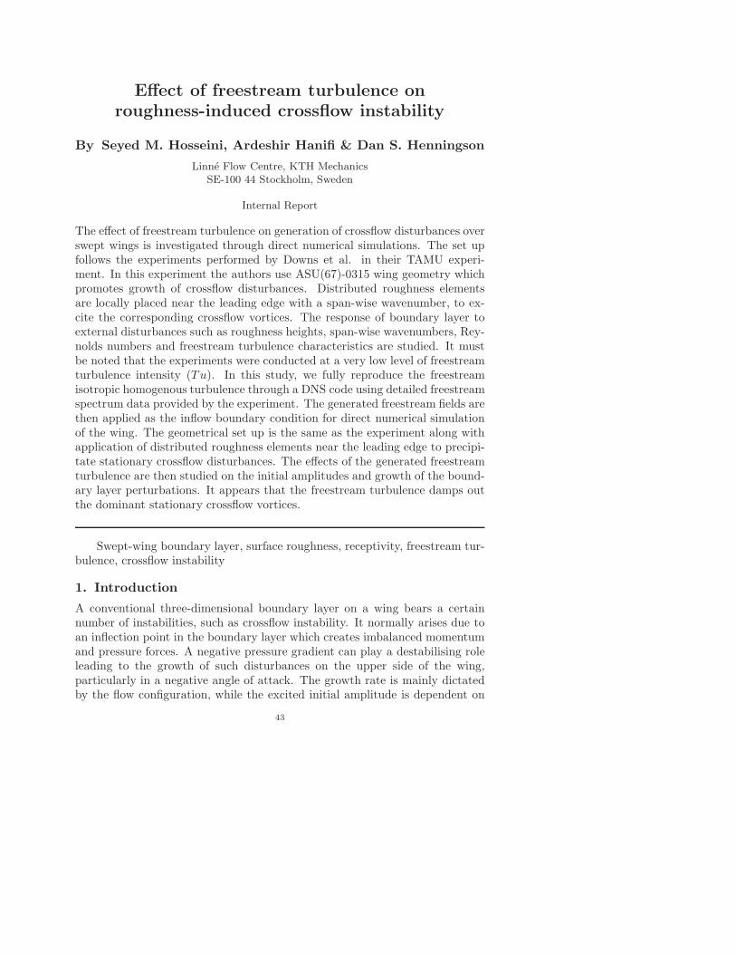
Figure 1. Swept ASU(67)-0315 wing, with sweep angle $#and the total incoming velocity Q#. The wing is at an angleof attack of $2.9$. (%, &, z) and (x, y, z) represent locally fit-ted curvilinear and cartesian coordinate systems respectively.(u", v#, w) and (u, v, w) are the corresponding defined veloci-ties in the introduced coordinates systems. The spectral ele-ments for DNS are depicted in red. The normalized streamwisevelocity contour lines from the RANS solution are shown rang-ing from 0.0 to 1.54 with a spacing of 0.024, which their valuesare used for the DNS baseflow. The blue lines represent thestreamlines of the baseflow.

a strong dependency of the transition mechanism on turbulent integral lengthscale. In their simulations the turbulent intensity was kept at a fixed value of6%.

In this study the experimental set up by Downs (2012) is considered inorder to numerically investigate the e!ect of freestream turbulence on cross-flow dominated flows. Direct numerical simulations are initially performed toextract the characteristics of stationary crossflow vortices. Furthermore, twotest cases from the experiment having di!erent levels of freestream turbulenceare selected. The perturbation field are generated via direct numerical simu-lations and then are fed in on top up of the inflow boundary condition andconvected downstream with the meanflow. At this stage the method of gen-erating freestream turbulence and the validity of direct numerical simulationsare to be examined.

2. Flow configuration

In the experiment a wing model is mounted vertically in the wind tunnel. Theincoming flow hits the leading edge at an angle of attack equal to ' = $2.9$.The wing is mounted at a sweep angle of $# = 45$ while keeping an infinitespan condition. The negative angle of attack along with the design of the wing

E!ect of freestream turbulence on roughness-induced crossflow instability 47

profile ASU(67)-0315 favors the growth of crossflow instabilities. The chordReynolds number is ReC = Q#C/( = 2.8 ' 106 which is based on the longswept chord, i.e. C = c/cos($) = 1.83m, while c, the unswept short chord, isdefined in figure 1. The coordinate system for the DNS is chosen to be along theshort chord, covering the upper side of the wing where measurements have beenperformed. The nose radius rn has been used in order to normalize lengths,and the velocities are normalized by the chordwise velocity of the freestreamvelocity, U#. The dictating Reynolds number is then:

Rern =U#rn(

, (1)

with ( being the kinematic viscosity of the fluid. The short chord Reynoldsnumber in the experiment is Rec = 1.4' 106, and in terms of the nose radiusis equal to Rern = 14676.1.

The freestream turbulence measurements have been documented. Note,that low levels of freestream turbulence is under consideration here in orderto resemble the free flight conditions. Noticeable discrepancies have been ob-served in the experiments by Reibert (1996), Hunt (2011), and free flight testof Carpenter et al. (2010) , conducted in di!erent environmental conditions.This mainly points to the responsibility of freestream turbulence. To furtheranalyze this problem, the freestream turbulence field is generated using directnumerical simulations (DNS).

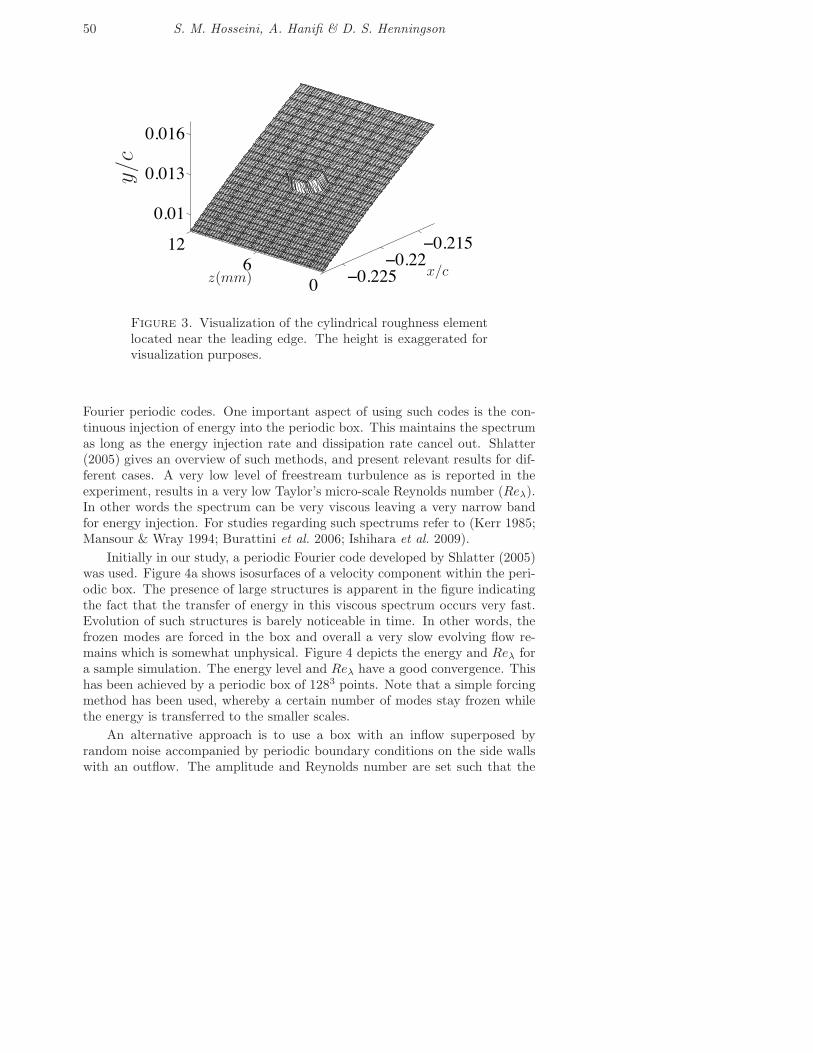
The roughness elements were also placed at x/c = 0.029 similar to the ex-periment with a spacing Lz = 12mm, where x denotes the chordwise direction(see figure 1). The wavelength of the naturally most unstable stationary cross-flow mode is )z = 12mm. The height and diameter of the elements were chosenas *r = 12µm and dr = 3mm respectively. Three simulations are performed,one without the freestream turbulence, and two including the freestream tur-bulence with di!erent turbulence length scales and intensities.

3. Direct numerical simulations

Direct numerical simulations were performed using the incompressible Navier-Stokes solver ‘Nek5000’ by Fischer et al. (2008), which uses the spectral elementmethod proposed by Patera (1984). Enabling geometrical flexibility using finiteelement methods combined with the accuracy provided by spectral methods arethe main advantages of using such codes. The spatial discretisation is obtainedby decomposing the physical domain into spectral elements. The solution tothe Navier-Stokes equations is approximated element-wise as a sum of Lagrangeinterpolants defined by an orthogonal basis of Legendre polynomials up to de-gree N. The following results have been obtained using N = 8. The presentSEM code is optimised for MPI based usage on supercomputers with thou-sands of processors (Tufo & Fischer 2001). Here, we have performed parallelcomputations on 8196 processors.

48 S. M. Hosseini, A. Hanifi & D. S. Henningson

Figure 2. The black lines represent the selected streamlinesbetween which a mesh refinement has been performed. Thered grid illustrates spectral elements near the leading edge.

3.1. Baseflow

The portion of the wing that is simulated is chosen such that it includes allthe interesting phenomena occurring on the wing, as depicted in figure 1. Thisentails the receptivity mechanism, initial perturbations growth, and the tran-sition to turbulence. The upstream inflow is placed in such a way as to ruleout any numerical contamination near the leading edge following the studiesby Tempelmann et al. (2012a,b). The upper bound also follows the same rec-ommendations by the mentioned studies. The downstream positions for theoutflow is set at x/c > 0.5 a bit further than the observed transition location(x/c > 0.4) in the experiment at the lowest turbulent intensity. A mesh gener-ator called gridgen-c developed by Sakov (2011) is used to generate the mesh.The upper and lower bounds conform to the streamlines extracted from com-plementary Reynolds Averaged Navier-Stokes (RANS) computations. A gridrefinement is performed between two streamlines regarding the higher recep-tivity near the leading edge as depicted by figure 2. An optimisation has beenperformed in order to find a good compromise between the number of elementsand element order. A higher element order naturally results in a tougher re-striction on the time step. In terms of obtaining the proper resolution, elementdistribution is more e"cient, compared to increasing the element order wherethe latter increases the resolution in non-essential areas.

In order to validate the computations of the baseflow, in addition to obtain-ing an optimum mesh resolution, a semi-three-dimensional simulation has beenperformed where the spanwise velocity component is computed via a passivescalar equation. Dirichlet boundary conditions are introduced at the inflow andthe upper and lower bounds of the domain. The corresponding velocities areextracted from the steady baseflow computed by RANS which is obtained bymanually prescribing the transition location on the upper side at x/c " 0.7 and

E!ect of freestream turbulence on roughness-induced crossflow instability 49

x/c " 0.01 on the lower-side. The specification of transition location, enablesthe RANS to avoid formation of separation bubbles near the pressure minimumlocations. Further, we choose zero-slip conditions at the wall while zero-stressboundary conditions are imposed at the outflow of the domain (x/c = 0.5).Periodic boundary conditions are also prescribed at the lateral boundaries. Atotal element number of 30000 elements are used for with a polynomial orderof N = 8.

3.2. Roughness induced crossflow vortices

The most unstable mode based on the linear stability theory as is reportedin the experiment has a spanwise periodicity of 12mm which is excited byan array of cylindrical roughness element. Numerically such periodicity canbe achieved by imposing periodic boundary conditions on lateral boundariesof the domain spaced at that specific periodic wavelength. The method hasbeen successfully tested in the studies by Tempelmann et al. (2012b). Theroughness shape is formed by displacement of the Gauss Lobatto Legendre(GLL) points normal to the surface, illustrated in figure 3. In the experimentby Downs (2012), the e!ect of turbulent intensity on the stationary crossflowvortices has been investigated for this configuration along with a number ofdi!erent levels of turbulent intensity. A sponge region is also used along withthe outflow boundary condition ramping the local velocity field to the DNScomputed from the semi-three-dimensional DNS. The usage of a sponge, regionfacilitates evading back-flows near the outflow region. Equation 2 dictates theforcing term present in the sponge region:

F (x, t) = Amax)(x)[Uf (x)$ U(X, t)], (2)

where Amax determines the maximum strength of sponge region, and )fis a step function (cf. Tempelmann et al. 2012b). Uf denotes the velocity fieldextracted from the semi-three-dimensional simulation. In other words, F (x, t)is proportional to the instantaneous local velocity. In our set up a maximumstrength of 2 has proven to be su"cient.

The parabolised stability equations introduced by Simen (1992) and Her-bert (1997) are common tools in stability analysis of convective unstable flows.An initial condition needs to be provided for such methods to predict the evolu-tion of perturbations. A detailed derivation of the linear and nonlinear methodcan be found in Bertolotti et al. (1992), Hanifi et al. (1994), and Herbert (1997).In this study the initial condition, form DNS, together with the baseflow is pro-vided to the NOLOT code (cf. Hein et al. 2000), to validate the evolution ofthe perturbations in order to establish an adequate mesh resolution.

3.3. Freestream turbulence

Di!erent methods have long existed for generating freestream isotropic tur-bulence. One typical tool of generating freestream turbulence is through the

50 S. M. Hosseini, A. Hanifi & D. S. Henningson

−0.225−0.22

−0.215

06

12

0.01

0.013

0.016y/c

x/cz(mm)

Figure 3. Visualization of the cylindrical roughness elementlocated near the leading edge. The height is exaggerated forvisualization purposes.

Fourier periodic codes. One important aspect of using such codes is the con-tinuous injection of energy into the periodic box. This maintains the spectrumas long as the energy injection rate and dissipation rate cancel out. Shlatter(2005) gives an overview of such methods, and present relevant results for dif-ferent cases. A very low level of freestream turbulence as is reported in theexperiment, results in a very low Taylor’s micro-scale Reynolds number (Re&).In other words the spectrum can be very viscous leaving a very narrow bandfor energy injection. For studies regarding such spectrums refer to (Kerr 1985;Mansour & Wray 1994; Burattini et al. 2006; Ishihara et al. 2009).

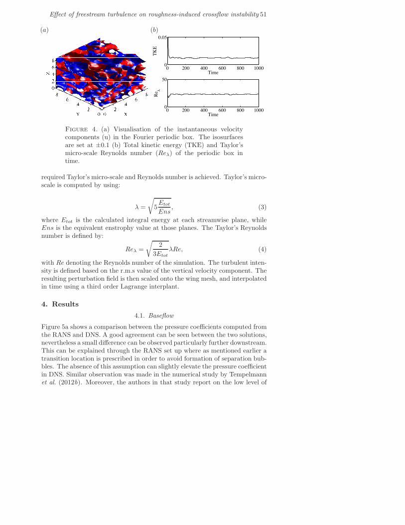
Initially in our study, a periodic Fourier code developed by Shlatter (2005)was used. Figure 4a shows isosurfaces of a velocity component within the peri-odic box. The presence of large structures is apparent in the figure indicatingthe fact that the transfer of energy in this viscous spectrum occurs very fast.Evolution of such structures is barely noticeable in time. In other words, thefrozen modes are forced in the box and overall a very slow evolving flow re-mains which is somewhat unphysical. Figure 4 depicts the energy and Re& fora sample simulation. The energy level and Re& have a good convergence. Thishas been achieved by a periodic box of 1283 points. Note that a simple forcingmethod has been used, whereby a certain number of modes stay frozen whilethe energy is transferred to the smaller scales.

An alternative approach is to use a box with an inflow superposed byrandom noise accompanied by periodic boundary conditions on the side wallswith an outflow. The amplitude and Reynolds number are set such that the

E!ect of freestream turbulence on roughness-induced crossflow instability 51

0 200 400 600 800 10000

0.05

Time

TKE

0 200 400 600 800 10000

50

Time

Reλ

(a) (b)

Figure 4. (a) Visualisation of the instantaneous velocitycomponents (u) in the Fourier periodic box. The isosurfacesare set at ±0.1 (b) Total kinetic energy (TKE) and Taylor’smicro-scale Reynolds number (Re&) of the periodic box intime.

required Taylor’s micro-scale and Reynolds number is achieved. Taylor’s micro-scale is computed by using:

) =

'

5Etot

Ens, (3)

where Etot is the calculated integral energy at each streamwise plane, whileEns is the equivalent enstrophy value at those planes. The Taylor’s Reynoldsnumber is defined by:

Re& =

'

2

3Etot)Re, (4)

with Re denoting the Reynolds number of the simulation. The turbulent inten-sity is defined based on the r.m.s value of the vertical velocity component. Theresulting perturbation field is then scaled onto the wing mesh, and interpolatedin time using a third order Lagrange interplant.

4. Results

4.1. Baseflow

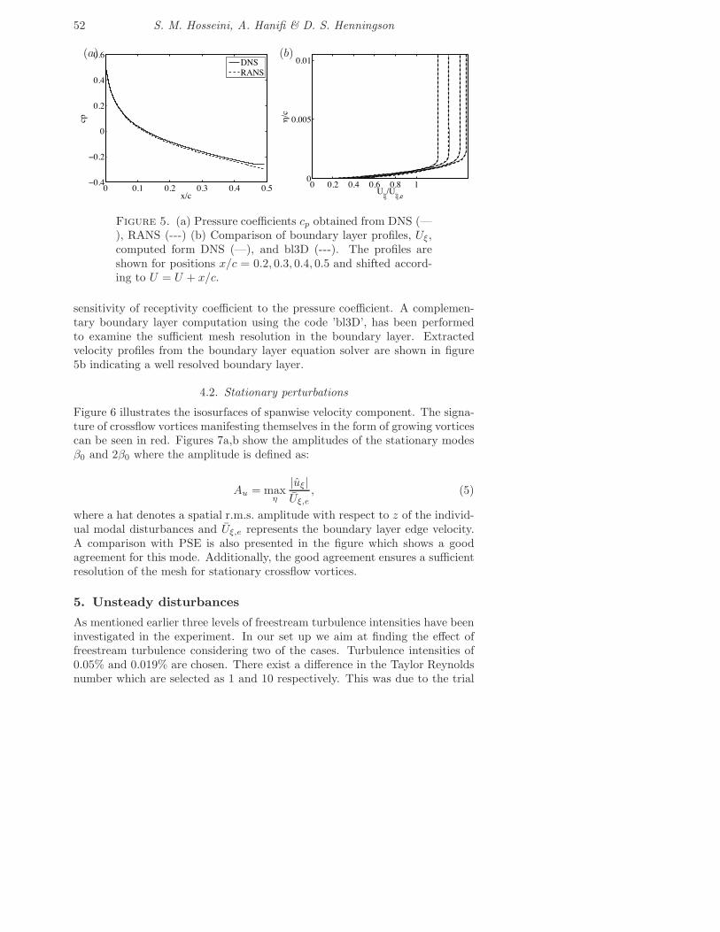
Figure 5a shows a comparison between the pressure coe"cients computed fromthe RANS and DNS. A good agreement can be seen between the two solutions,nevertheless a small di!erence can be observed particularly further downstream.This can be explained through the RANS set up where as mentioned earlier atransition location is prescribed in order to avoid formation of separation bub-bles. The absence of this assumption can slightly elevate the pressure coe"cientin DNS. Similar observation was made in the numerical study by Tempelmannet al. (2012b). Moreover, the authors in that study report on the low level of

52 S. M. Hosseini, A. Hanifi & D. S. Henningson

0 0.1 0.2 0.3 0.4 0.5−0.4

−0.2

0

0.2

0.4

0.6

x/c

cp

DNSRANS

0 0.2 0.4 0.6 0.8 10

0.005

0.01

Uξ/U

ξ,e

η/c

(a) (b)

Figure 5. (a) Pressure coe"cients cp obtained from DNS (—), RANS (---) (b) Comparison of boundary layer profiles, U",computed form DNS (—), and bl3D (---). The profiles areshown for positions x/c = 0.2, 0.3, 0.4, 0.5 and shifted accord-ing to U = U + x/c.

sensitivity of receptivity coe"cient to the pressure coe"cient. A complemen-tary boundary layer computation using the code ’bl3D’, has been performedto examine the su"cient mesh resolution in the boundary layer. Extractedvelocity profiles from the boundary layer equation solver are shown in figure5b indicating a well resolved boundary layer.

4.2. Stationary perturbations

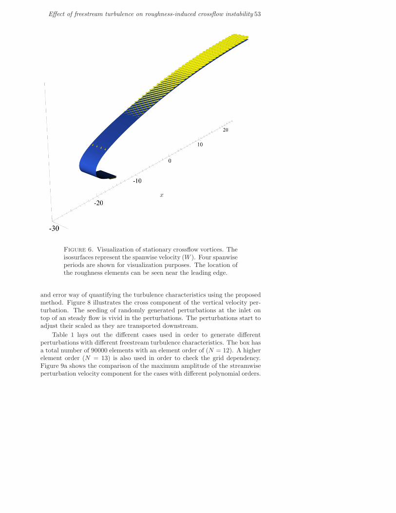
Figure 6 illustrates the isosurfaces of spanwise velocity component. The signa-ture of crossflow vortices manifesting themselves in the form of growing vorticescan be seen in red. Figures 7a,b show the amplitudes of the stationary modes!0 and 2!0 where the amplitude is defined as:

Au = max#

|u"|

U",e, (5)

where a hat denotes a spatial r.m.s. amplitude with respect to z of the individ-ual modal disturbances and U",e represents the boundary layer edge velocity.A comparison with PSE is also presented in the figure which shows a goodagreement for this mode. Additionally, the good agreement ensures a su"cientresolution of the mesh for stationary crossflow vortices.

5. Unsteady disturbances

As mentioned earlier three levels of freestream turbulence intensities have beeninvestigated in the experiment. In our set up we aim at finding the e!ect offreestream turbulence considering two of the cases. Turbulence intensities of0.05% and 0.019% are chosen. There exist a di!erence in the Taylor Reynoldsnumber which are selected as 1 and 10 respectively. This was due to the trial

E!ect of freestream turbulence on roughness-induced crossflow instability 53

x

Figure 6. Visualization of stationary crossflow vortices. Theisosurfaces represent the spanwise velocity (W ). Four spanwiseperiods are shown for visualization purposes. The location ofthe roughness elements can be seen near the leading edge.

and error way of quantifying the turbulence characteristics using the proposedmethod. Figure 8 illustrates the cross component of the vertical velocity per-turbation. The seeding of randomly generated perturbations at the inlet ontop of an steady flow is vivid in the perturbations. The perturbations start toadjust their scaled as they are transported downstream.

Table 1 lays out the di!erent cases used in order to generate di!erentperturbations with di!erent freestream turbulence characteristics. The box hasa total number of 90000 elements with an element order of (N = 12). A higherelement order (N = 13) is also used in order to check the grid dependency.Figure 9a shows the comparison of the maximum amplitude of the streamwiseperturbation velocity component for the cases with di!erent polynomial orders.

54 S. M. Hosseini, A. Hanifi & D. S. Henningson

0 0.1 0.2 0.3 0.4 0.510−4

10−3

10−2

10−1

100

x/c

Au

linear PSEDNSnonlinear PSE

0 0.1 0.2 0.3 0.4 0.510−4

10−3

10−2

10−1

100

x/c

Au

linear PSEDNSnonlinear PSE

(a) (b)

Figure 7. Amplitude Au of the stationary modes in the ab-sence of unsteady perturbations for (a) fundamental mode !0and (b) 2!0.

X

Y

Z

Figure 8. Isosurfaces of vertical velocity perturbations v!,drawn at ±0.0001|v!|.

A good level of agreement can be observed between the maximum perturbationamplitude. The same trend can be seen between the energy levels as depictedin figure 9b ensuring su"cient resolution.

E!ect of freestream turbulence on roughness-induced crossflow instability 55

Table 1. Selected cases with di!erent turbulent characteristics.

Case Turbulent Integral Taylor’s Re&Name intensity length scale micro scale

Tu L )Tu5 0.05% 48mm 1.6mm 1Tu19 0.19% 36mm 4.5mm 10

10−1 10010−5

10−4

10−3

10−2

10−1

X

u max

O11O13

10−1 10010−8

10−7

10−6

10−5

10−4

X

Ener

gy

O11O13

(a) (b)

Figure 9. (a) Maximum instantaneous streamwise perturba-tion (umax) along the streamwise direction (b) Computed en-ergy along the streamwise direction for two mesh resolutions.

10−1 10010−5

10−4

10−3

10−2

10−1

X

Am

p max

uvw

10−1 100

10−5

10−4

10−3

10−2

10−1

X

Am

p

umax

Etot

Ens

(a) (b)

Figure 10. (a) Instantaneous components of velocity pertur-bation within the periodic box (b) Computed energy, enstro-phy from streamwise perturbation.

To determine the level of isotropy in the generated turbulence field threevelocity components are depicted in figure 10 for the set up case Tu5. Agood level of isotropy can be seen among the di!erent velocity components.A quick look at the velocity isosurfaces reveals the way the perturbations andvorticity decay along the streamwise direction. A linear trend can be seen

56 S. M. Hosseini, A. Hanifi & D. S. Henningson

0 1 2 3 4 50

10

20

30

40

XRe

λ

Figure 11. Taylor’s microscale Reynolds number Re& com-puted within the periodic box.

x

Figure 12. Isosurfaces of the instantaneous perturbation ve-locity u!. The levels of isosurfaces are set at ±0.0004|u!|.

which is similar to what is observed in the experiments. Figure 10b showsthe computed instantaneous enstrophy and energy at each plane along thestreamwise direction. The computed values are then used in order to computeTaylor’s Reynolds number, Re&, see figure 11. The computed flow is now scaledonto the grid of the wing geometry. Note the spanwise length is chosen such asto accommodate the integral length scale of the considered case. Furthermorea third order Lagrange interpolation in time is performed among the previouslysaved freestream perturbations.

Figure 12 depicts the streamwise velocity perturbation field belonging tothe two studied cases. The dominance of the crossflow vortices can be seen nearthe outflow. No transition has been observed for the T5 case. E!ect of di!erentturbulent perturbations on amplitudes of the stationary crossflow vortices hasbeen compared in figure 13. An apparent damping of the stationary crossflowvortices can be seen with introduction of freestream turbulence for Tu5 case for

E!ect of freestream turbulence on roughness-induced crossflow instability 57

0 0.1 0.2 0.3 0.40.01

0.1

x/c

Au

Tu0Tu5Tu19

0 0.1 0.2 0.3 0.4

0.01

x/c

Au

Tu0Tu5Tu19

(a) (b)

Figure 13. Amplitude evolution of steady disturbances de-picted for the three studied case (a) fundamental mode !0 and(b) 2!0.

the primary !0(12mm) mode. It must also be noted that in none of the casesthe excited initial amplitudes by the roughness element shows any tangibledi!erence. For the stationary 2!0 the di!erence in amplitudes is not as strongas the !0 mode.

6. Conclusions & Outlook

Direct numerical simulations (DNS) have been performed in order to investigatethe role of freestream perturbations at a very low turbulence level on crossflowinstability. The studied cases follow the experiments conducted by Downset al. in Texas A&M University. In their experiment the authors documentthe freestream perturbations to a great detail, reporting freestream turbulencelength scales, intensity, spectrum, etc. This enables the numerical studies tofully reproduce the freestream perturbations in such analysis. The experimentused ASU(67)-0315 wing geometry designed to promote crossflow instability.In our study we approach the reported values in generating the low intensityfreestream turbulence. A DNS code (nek5000) has been used in order to gener-ate the perturbation field. The perturbations are then scaled and interpolatedonto the wing mesh.

Two di!erent set of freestream turbulence characteristics have been chosen.So far in the simulations, it has been observed that the growth rate of the sta-tionary crossflow modes assumes a lower value in proportion to the freestreamturbulence intensity level. However the results are so far preliminary and partof an ongoing work and further convergence of the simulated cases are required.Additional parameters must also be looked at, such as the spectrum of the per-turbations, secondary instabilities, etc. It must be noted that transition hasnot been observed in any of the case with freestream turbulence.

The authors wish to thank Philipp Schlatter for fruitful discussions andvaluable comments. Computer time provided by SNIC (Swedish National

58 S. M. Hosseini, A. Hanifi & D. S. Henningson

Infrastructure for Computing) at the Center for Parallel Computers (PDC),KTH, is gratefully acknowledged. This work has been supported by the Euro-pean Commission through the FP7 project ‘RECEPT’ (Grant Agreement no.ACPO-GA-2010-265094)

E!ect of freestream turbulence on roughness-induced crossflow instability 59

References

Bertolotti, F. P., Herbert, T. & Spalart, P. R. 1992 Linear and nonlinearstability of the Blasius boundary layer. J. Fluid Mech. 242, 441–474.

Bippes, H. 1999 Basic experiments on transition in three-dimensional boundary layersdominated by crossflow instability. Progress in Aerospace Sciences 35, 363–412.

Brandt, L., Schlatter, P. & Henningson, D. 2004 Transition in boundary layerssubject to free-stream turbulence. J. Fluid Mech. 517, 167–198.

Burattini, P., Lavoie, P., Agrawal, A., Djenidi, L. & Antonia, R. A. 2006Power law of decaying homogeneous isotropic turbulence at low reynolds number.Phys. Rev. E 73, 066304.

Carpenter, A. L., Saric, W. S. & Reed, H. L. 2010 Roughness receptivity inswept-wing boundary layers-experiments. Int. J. Eng. Syst. Model. Simul pp.128–138.

Downs, R. S. 2012 Environmental influences on crossflow instability. PhD thesis,Texas A&M University.

Fischer, P. F., Lottes, J. W. & Kerkemeier, S. G. 2008 nek5000 Web page.Http://nek5000.mcs.anl.gov.

Fransson, J. H. M., Matsubara, M. & Alfredsson, P. H. 2005 Transition in-duced by free-stream turbulence. J. Fluid Mech. 527, 1–25.

Grosch, C. E. & Salwen, H. 1978 The continuous spectrum of the Orr-Sommerfeldequation. Part 1. The spectrum and the eigenfunctions. J. Fluid Mech. 87, 33–54.

Hanifi, A., Henningson, D. S., Hein, S., Bertolotti, F. P . & Simen, M.

1994 Linear non-local instability analysis - the linear NOLOT code. FFA TN1994-54.

Hein, S., Hanifi, A. & Casalis, G. 2000 Nonlinear transition prediction. In Proceed-ings of the European Congress on Computational Methods in Applied Sciencesand Engineering .

Herbert, T. 1997 Parabolized Stability Equations. Annu. Rev. Fluid Mech. 29, 245–283.

Hunt, L. E. 2011 Boundary-layer receptivity to three-dimensional roughness arrayson a swept-wing. PhD thesis, Texas A&M University.

Ishihara, T., Gotoh, T. & Kaneda, Y. 2009 Study of high—reynolds numberisotropic turbulence by direct numerical simulation. Annu. Rev. Fluid Mech. 41,165–180.

Jacobs, R. G. & Durbin, P. A. 2001 Simulations of bypass transition. J. FluidMech., vol. 428, pp. 185-212 428, 185–212.

Jonas, P., Mazur, O. & Uruba, V. 2000 On the receptivity of the by-pass transitionto the length scale of the outer stream turbulence. Eur. J. Mech B/Fluids 19,707–722.

Kendall, J.M. 1991 Studies on laminar boundary-layer receptivity to freestreamturbulence near a leading edge. See Reda et al. pp. 23–30.

Kendall, J.M. 1998 Experiments on boundary-layer receptivity to freestream tur-bulence. AIAA Paper 98-0530 .

Kerr, R. 1985 Higher-order derivative correlations and the alignment of small-scalestructures in isotropic turbulence. J. Fluid Mech. 153, 31–58.

Kurian, T., Fransson, J. H. M. & Alfredsson, P. H. 2011 Boundary layerreceptivity to free-stream turbulence and surface roughness over a swept flatplate. Phys. Fluids 23, 034107.

Mansour, N. N. & Wray, A. A. 1994 Decay of isotropic turbulence at low reynoldsnumber. Phys. Fluids 6(2), 808–815.

Matsubara, M. & Alfredsson, P. H. 2001 Boundary-layer transition under free-stream turbulence. J. Fluid Mech. 430, 149–168.

Ovchinnikov, V., Choudhari, M. M. & Piomelli, U. 2008 Numerical simulationof boundary-layer bypass transition due to high-amplitude free-stream turbu-lence. J. Fluid Mech. 613, 135–169.

Patera, A. T. 1984 A Spectral Element Method for Fluid Dynamics: Laminar Flowin a Channel Expansion. J. Comp. Phys. 54, 468–488.

Reibert, M. S. 1996 Nonlinear stability, saturation, and transition in crossflow-dominated boundary layers. PhD thesis, Arizona State University.

Rogler, H. 1978 The interaction between vortex-array representation of free-streamturbulence and semi-infinite flat plates. J. Fluid Mech. 87, 583–606.

Rogler, H. L. & Reshotko, E. 1975 Disturbances in boundary layer introducedby a low intensity array of vortices. J. APPL. MATH 28.

Sakov, P. 2011 gridgen-c - an orthogonal grid generator based on the crdt algorithm(by conformal mapping). http://code.google.com/p/gridgen-c/.

Saric, W. S., Reed, H. L. & Kerschen, E. J. 2002 Boundary-Layer Receptivityto Freestream Disturbances. Annu. Rev. Fluid Mech. 34, 291–319.

Schrader, L. U., Amin, S. & Brandt, L. 2010 Transition to turbulence in theboundary layer over a smooth and rough swept plate exposed to free-streamturbulence. J. Fluid Mech. 646.

Shahinfar, S. 2013 An experimental study on streamwise streaks in transitionalboundary layer. PhD thesis, KTH Stockholm.

Shlatter, P. C. 2005 Large-eddy simulation of transition and turbulence in wall-bounded shear flow. PhD thesis, Swiss Federal Institute of Technology.

Simen, M. 1992 Local and non-local stability theory of spatially varying flows. InInstability, Transition and Turbulence, pp. 181–195. Springer Verlag.

Tempelmann, D., Hanifi, A. & Henningson, D. S. 2012a Swept-wing boundary-layer receptivity. J. Fluid Mech. 700, 490–501.

Tempelmann, D., Schrader, L.-U., Hanifi, A., Brandt, L. & Henningson,

D. S. 2012b Swept wing boundary-layer receptivity to localised surface rough-ness. J. Fluid Mech. 711, 516–544.

Tufo, H. M. & Fischer, P. F. 2001 Fast Parallel Direct Solvers for Coarse GridProblems. J. Parallel Distrib. Comput. 61 (2), 151–177.