Effect of Blowing Ratio on the Nusselt Number and Film Cooling Effectiveness Distributions of a Showerhead Film Cooled Blade in a Transonic Cascade Ashley R. Guy Thesis submitted to the faculty of the Virginia Polytechnic Institute and State University in partial fulfillment of the requirements for the degree of Master’s of Science in Mechanical Engineering Dr. Wing Ng, Chair Dr. Thomas Diller Dr. Brian Vick July 16, 2007 Blacksburg, Virginia Keywords: Film Cooling, Turbine Blade, Heat Transfer, Cascade
Transcript
Effect of Blowing Ratio on the Nusselt Number and Film Cooling Effectiveness Distributions of a Showerhead
Film Cooled Blade in a Transonic Cascade
Ashley R. Guy
Thesis submitted to the faculty of the Virginia Polytechnic Institute and State University
in partial fulfillment of the requirements for the degree of
Master’s of Science in
Mechanical Engineering
Dr. Wing Ng, Chair Dr. Thomas Diller
Dr. Brian Vick
July 16, 2007 Blacksburg, Virginia
Keywords: Film Cooling, Turbine Blade, Heat Transfer, Cascade
ii
Effect of Blowing Ratio on the Nusselt Number and Film Cooling Effectiveness Distributions of a Showerhead Film Cooled Blade in a Transonic Cascade
Ashley R. Guy Virginia Polytechnic Institute and State University, 2007
Advisor: Dr. Wing F. Ng
Thesis Abstract To increase the efficiency of gas turbine engines, higher turbine operating
temperatures have been employed. In order to keep the turbine component temperatures
below their melting point, air from the compressor section of the turbine is ejected over
the surface of the blade to provide a protective shroud of cooler air over the surface of the
blades. Film cooling performance is difficult to predict analytically or computationally—
for this reason, experiments are needed to properly characterize the performance of
designed cooling schemes.
In this study, a first stage turbine blade with three rows of showerhead cooling
holes was instrumented with heat flux gages to experimentally characterize the Nusselt
Number and film cooling effectiveness distributions over the surface of the blade. The
blade was arranged in a two-dimensional, linear cascade in a transonic, blowdown-type
wind tunnel. The wind tunnel freestream conditions were varied over two exit Mach
numbers, Me=0.78 and Me=1.01, with an inlet freestream turbulence intensity of 12%
with an integral length scale normalized by blade chord of 0.26 generated by a passive
mesh turbulence grid. The coolant conditions were varied by changing the ratio of
coolant to freestream mass flux, blowing ratio, over three values: BR=0.60, 1.0, and 1.5.
Film cooling performance is characterized by experimental results in terms of
Nusselt number and film cooling effectiveness distributions. These distributions are the
result of five measurement locations over an extent of s/d=-32 on the pressure side to
s/d=33 on the suction side. Film cooling was found to increase Nusselt number over the
entire measurement domain, and increasing the blowing ratio also increased the Nusselt
number. Of the blowing ratios tested, a blowing ratio of 1.0 was found to have superior
heat load reduction performance at both freestream conditions tested.
iii
Acknowledgements This study was sponsored by Solar Turbines and conducted under the direction of
Drs. Hee-Koo Moon and Luzeng Zhang. I would like to thank them for their support and
guidance over the duration of this project. I would also like to thank Drs. Mark Polanka
and Richard Anthony of the Air Force Research Laboratory for the manufacture of the
thin film gages that were critical to this project. Thanks to the Aerojet corporation for
providing funding for my fellowship and their continued support of Virginia Tech
Mechanical Engineering.
The members of my committee have been invaluable to the success of this
project. Starting with his teaching, and continuing through the opportunities he has given
me to work on many research projects during the past several years, Dr. Ng has been a
great mentor over the course of my academic career. He is a truly wonderful manager
that gives a great deal of trust and responsibility to his students. Without Dr. Diller’s
advice and judgment, this project could not have proven a success. His experience was
always there for the team at critical junctions of this project because of the generosity
with which he gives his time. Dr. Vick is an unparalleled teacher. One of the most
important attitudes I will take away from Virginia Tech comes from Dr. Vick’s teaching
philosophy-make sure your understand the fundamentals in detail.
My research team has been the most valuable part of my work. This project was
truly a team effort, and without Shakeel Nassir, Trey Bolchoz, and Jeff Carullo I would
simply not be graduating. Words cannot express my gratitude. I would also like to thank
the M.E. office and shop for all of their help. Bill Songer has proved and invaluable part
of all the projects I have taken part in, and both his work and humor have gotten me
through.
I would like to thank my family and friends. My family has given me everything
that I could ever expect and more. There is no way to thank your family the way they
deserve, but I hope that this thesis and degree will help to show that a bit of their hard
work has paid off. To my friends that have become my extended family, I cannot say
enough.
iv
My parents, Bill and Raye Guy, grandma, Barbara Shiley, and aunt, Evelene
Curry, made it possible for my sister, Margaret, and I to attend Virginia Tech. Nowhere
on earth would have suited me better and I am grateful for the opportunity.
I would also like to extend my gratitude to the Virginia Tech community. The
strength, sensitivity, and fortitude that has been shown is something we can all be proud
of. Anyone who has experienced this community could have told you that we have
something special--even before the tragic events of this past April. While we all share a
deep sense of sorrow, I think we can be proud that we have shown what it means to be
Virginia Tech.
v
Attribution This research project was the result of a team effort, and the paper that forms the
body of this thesis is coauthored by the members of this research team. Included in the
“Attribution” section is a description of the author’s contribution to this work.
Shakeel Nasir- M.S.M.E. (Department of Mechanical Engineering), Virginia Tech is a
Ph.D. candidate in mechanical engineering and a member of the author’s research team
that undertook this project. Shakeel assisted with the design of experiment,
manufacturing of test articles, installation, data reduction, and with the review of
literature as part of the requirements of his studies.
Ruford Bolchoz- B.S.M.E. (Department of Mechanical Engineering), Virginia Tech is a
master’s candidate in mechanical engineering and a member of the author’s research
team that undertook this project. Ruford built the film cooling circuit that was used in
this project and authored the checklists provided in Appendix A. He also helped with
running the experiment and data reduction.
Prof. Wing F. Ng- Ph.D. (Department of Mechanical Engineering), Virginia Tech is the
primary Advisor and Committee Chair. His leadership and advice guided the team
throughout this work.
Luzeng Zhang- Ph.D. (Senior Principal Engineer, Heat Transfer), Solar Turbines Inc.
Hee K. Moon- Ph.D. (Group Manager, Heat Transfer), Solar Turbines Inc. Drs. Zhang
and Moon provided the design of the film cooled blade that was used in this testing.
They also helped the team by discussing the “three temperature problem” associated with
film cooling research. Solar Turbines Inc. provided the funding for this work.
vi
Table of Contents Title Page ............................................................................................................................. i
Thesis Abstract.................................................................................................................... ii
Acknowledgements............................................................................................................ iii
Attribution........................................................................................................................... v
Table of Contents............................................................................................................... vi
List of Figures .................................................................................................................. viii
List of Tables ...................................................................................................................... x
Preface................................................................................................................................ xi
Effect of Blowing Ratio on the Nusselt Number and Film Cooling Effectiveness
Distributions of a Showerhead Film Cooled Blade in a Transonic Cascade ...................... 1
Table E-5. Me=1.01, Nu ................................................................................................. 47
Table E-6. Me =1.01, Nu/Nu0 ......................................................................................... 47
Table E-7. Me =1.01, η ................................................................................................... 47
Table E-8. Me =1.01, Δq”red ........................................................................................... 47
xi
Preface In the drive to increase the efficiency of gas turbine engines, higher operating
temperatures have been employed by engine designers. The operating temperature can
be above engine component melting points. A method used to protect components is film
cooling. Turbine blades are equipped with a plenum and an array of cooling holes.
Cooler air from the compressor section of the engine is ejected over the blade surface
forming a shroud of air that protects the engine components from the hot gas exiting the
combustor.
Because this process involves the mixing of gases at different speeds, densities,
temperatures, and flow directions at high freestream turbulence, it has been challenging
to model analytically or to predict with current CFD methods. Experimental studies are
necessary to provide engineers with the adequate parameters needed to predict the
performance and lifespan of the components they design.
The study of film cooling is inherently a study in design balance. When
considering cooling system design on an engine scale, increasing the amount of coolant
supplied yields a cooler blade that will last longer, but decreases engine core flow--
diminishing efficiency. Interestingly, when contemplating the physics of film cooling,
balance is also the key to developing an effective design. Increasing the amount of
coolant injected reduces the driving temperature of heat transfer, but more coolant
augments boundary layer disturbance--providing a higher heat transfer coefficient. So, if
the designer does not balance the decrease in driving potential with the increase in heat
transfer coefficient, he or she will not decrease the heat load experienced by the engine
component.
This thesis, on a fundamental level, explores the aspects of film cooling balance
by measuring film cooling performance at different rates of coolant injection at varying
freestream flow conditions. The driving temperature of heat transfer is presented in terms
of film cooling effectiveness and the heat transfer coefficient is provided as the Nusselt
number. The effect of the amount of coolant supplied is studied by varying the blowing
ratio. The effect of the freestream is examined by measuring film cooling performance at
two Mach numbers. This thesis is arranged in a conference paper format with subsequent
appendices attached to expand and support ideas presented in the paper.
1
Effect of Blowing Ratio on the Nusselt Number and Film Cooling Effectiveness Distributions of a Showerhead Film Cooled Blade in a Transonic Cascade
A. R. Guy, S. Nasir, R. Bolchoz, and W.F. Ng Mechanical Engineering Department
Virginia Polytechnic Institute and State University Blacksburg, VA 24061
L.J. Zhang and H.K. Moon Solar Turbines Inc.
San Diego, CA 92101
Abstract This paper investigates the effect of blowing ratio on the film cooling
performance of a showerhead film cooled first stage turbine blade. The blade was
instrumented with double-sided thin film heat flux gages to experimentally characterize
the Nusselt number and film cooling effectiveness distributions over the surface of the
blade. The blade was arranged in a two-dimensional, linear cascade within a transonic,
blowdown type wind tunnel. The wind tunnel freestream conditions were varied over
two exit Mach numbers, Me=0.78 and Me=1.01, with an inlet freestream turbulence
intensity of 12% , with an integral length scale normalized by blade chord of 0.26
generated by a passive, mesh turbulence grid. The coolant conditions were varied by
changing the ratio of coolant to freestream mass flux, blowing ratio, over three values,
BR=0.60, 1.0, and 1.5 while keeping a density ratio of 1.7.
Experimental results show that ingestion of freestream flow into the showerhead
cooling plenum can occur below a blowing ratio of 0.6. Film cooling increases Nusselt
number over the uncooled case and increasing the blowing ratio also increases Nusselt
number. At a blowing ratio of 1.5 and Me=1.01 a large drop in effectiveness just
downstream of injection on both the pressure and suction surfaces is evidence of jet
liftoff. The blowing ratio of 1.0 was found to have superior heat load reduction over the
blade surface at both freestream conditions tested. The blowing ratio of 1.0 reduced the
heat load by as much as 39% and 32% at Me=0.78 and 1.01, respectively.
2
Nomenclature A area
BR blowing ratio C blade true chord d cooling hole diameter
DR density ratio h heat transfer coefficient k conductivity l thickness of gage
LS integral length scale M Mach Number m& mass flow rate Nu Nusselt Number P blade pitch p cooling hole pitch
PS pressure side q” heat flux r turbulent recovery factor
Re Reynolds Number s surface distance
SS suction side T temperature Tu freestream turbulence intensity in the streamwise direction U velocity
Greek φ overall film cooling effectiveness α spanwise cooling hole angle γ specific heat ratio η film cooling effectiveness ρ density
Subscripts 0 total ∞ freestream aw adiabatic wall temperature b backwall thermocouple c coolant e exit f film cooling i inlet
loc local o no film cooling r recovery
red reduction w wall, Pt TFG surface
3
Introduction In the drive to increase the efficiency of gas turbine engines, higher and higher
engine operating temperatures have been employed by engine manufacturers. These
temperatures can become so high that they are above the melting temperature engine
components themselves. A method used to protect the components from melting is film
cooling. In this method, turbine blades are equipped with a plenum and an array of
cooling holes arranged over their surface. Cooler air from the compressor section of the
engine is blown through these holes where it forms a thin film of cool air separating the
engine components from the hot gas path. The cooling air protects the blade from the
extreme temperatures of the gases that have just left the combustion portion of the
engine.
Because this process involves the mixing of gases at different speeds, densities,
temperatures, and flow directions, it has been extremely challenging to model
analytically or to predict with current CFD methods. For this reason, experimental
studies are necessary to provide engineers with the adequate parameters to predict the
performance and lifespan of the components they design.
The current study presents experimental results examining the effect of blowing
ratio on the film cooling performance of a showerhead film cooled turbine blade at
different Mach numbers. The performance of film cooling has been characterized by
measuring the Nusselt number and film cooling effectiveness distribution over the
surface of a showerhead film cooled blade.
Summary of Literature Film Cooling is a broad, mature topic and its varied applications have been
studied in the literature for some time. The basic film cooling physics are described by
Goldstein [1]. Bogard and Thole [2] and Han et al. [3] have compiled much of the
current work on film cooling as it applies to the gas turbine field. The current
experimental work concerns a turbine blade in a high speed environment. Therefore, the
literature review has been limited to airfoils in both low and high speed environments.
Literature is presented in increasing relevance beginning with low speed vane and blade
studies and concluding with high speed vane and blade experiments.
4
Low Speed Vane. Ames [4] studied the effects of turbulence and rate of coolant
injection on a film cooled C3X vane in a low speed facility at two Reynolds numbers.
Several film cooling geometries were studied, but the showerhead cooled vane results are
of interest to this study. Ames used thermocouples to measure the surface temperature
distribution with foil heaters supplying heat flux and a finite element analysis to correct
for two-dimensional internal conduction. The results showed that film cooling
augmented Stanton number in the both the laminar and turbulent regions of the vane with
more augmentation in the laminar region. Increasing the rate of coolant injection
increased the levels of Stanton number augmentation. The effect of coolant injection rate
on effectiveness was shown to be greater than the effect of Reynolds number on
effectiveness. The effect of freestream turbulence was observed to reduce the levels of
film cooling effectiveness and also quicken the dissipation of cooling effectiveness.
Low Speed Blade. A study of coolant density ratio and the impact of an
upstream wake were studied in a low speed linear fully film cooled blade cascade by Ou
et al.[5] and Mehendale et al.[6]. Heat transfer coefficient is reported by [6], while
effectiveness and heat load reduction are presented by [7]. Density ratio was varied by
using air and CO2 as the two coolant gases and a spoked wheel wake generator simulated
blades passing an upstream wake. Film cooling increased the heat transfer coefficient
over the surface of the blade and it was found that cooling injection had a more dominant
effect on heat transfer coefficient than the addition of the upstream wake. An increase in
the mass flux ratio, blowing ratio, was seen to increase heat transfer coefficient. The
addition of the wake reduced film cooling effectiveness. Different blowing ratios were
seen to provide the highest effectiveness levels for air and CO2 injection. However, it
was noted that reported values of effectiveness for the higher density, CO2, case could be
conservative due to the specific heat differences between air and CO2. The best blowing
ratio in the range of 0.4-1.2 studied, in terms of heat load reduction, was determined to be
0.8 and 1.2 for air and CO2, respectively. The addition of grid turbulence on film
cooling performance was studied in the same facility by Ekkad et al.[6]. Superimposing
turbulence from a grid on a wake was found to increase heat transfer coefficients and
decrease film cooling effectiveness. However, at a high enough level of freestream
5
turbulence, the unsteady wake was shown to have negligible effect on film cooling
performance.
High Speed Vane. The effects of varying Reynolds number, Mach number,
coolant injection rate, and coolant to temperature ratio were studied on a showerhead
cooled C3X vane in a transonic, linear cascade by Turner et al. [8]. Increasing the rate of
coolant injection was seen to increase the heat transfer coefficient. Increases in Reynolds
number in the film cooled case were also seen to augment the film cooled heat transfer
coefficient. It was noted that the addition of film cooling had a definite effect on heat
transfer coefficient in the laminar region, but after transition the effect of film cooling
was negligible. While not dramatically, film cooling was shown to move the location of
laminar to turbulent transition farther upstream.
Drost and Bölcs [9] studied the effect of varying Mach number, density ratio,
blowing ratio, and freestream turbulence on a high speed vane. The transient liquid
crystal technique was used to determine h and η. An increase in effectiveness was
observed with an increase in blowing ratio. For a double row of film cooling holes on the
suction surface, between blowing ratios of 1.11 and 1.77 jet liftoff was observed. For
increasing blowing ratio, increasing heat transfer coefficient augmentation was also
observed. On the suction side, the reduction of heat load is higher closer to injection for
lower blowing ratios and higher farther downstream of injection for higher blowing
ratios. For the pressure side, a heat load increase was seen for blowing ratios above 1.3.
Guo et al. [10] used platinum thin film gages on a semi-infinite substrate in a
transonic annular cascade to measure the effect of film cooling on a fully cooled nozzle
guide vane. Foreign gas with specific heat properties similar to air was used to match the
density ratio seen in a gas turbine. Augmentation of heat transfer coefficient due to
cooling was observed over the entire pressure surface and some of the suction surface.
Heat transfer coefficient levels below that of uncooled data are reasoned to be the result
of a thicker boundary layer. Effectiveness was higher on the pressure side where more
rows of coolant injection were present and decreased after the last row of cooling holes.
Piccini et al. [11] developed a type of double-sided thin film gage by adding a
thermocouple beneath the thin film gages used by [10]. A variation of this type of
double-sided gage is used in this work.
6
High Speed Blade. Camci and Arts [12] measured heat transfer coefficient over
a film cooled blade in a short duration, high speed facility with thin film gages mounted
on a semi-infinite, Macor blade. The effect of internal conduction in the blade plenum
region was accounted for by reporting a higher uncertainty closer to the plenum region.
Increasing the coolant mass flow was observed to decrease the heat transfer coefficient
and cooled heat transfer coefficient levels were observed below the levels of an uncooled
case.
Rigby et al. [13] tested a range of film cooling geometries, blowing ratios, and the
effect of upstream passing shocks and wakes on the film cooling performance in a two
dimensional linear cascade. On the suction surface, increasing the blowing ratio was
noted to decrease heat transfer coefficient below the uncooled case. Also on the suction
surface, film coolant liftoff was assumed because of a drop of effectiveness between a
blowing ratio of 1.0 and 1.5. Schlieren photography captured this coolant liftoff. Shock
and bar passing were seen to decrease film cooling effectiveness.
The geometry studied by [13] was tested in MIT’s blowdown turbine test facility
in a full rotating stage by Abhari and Epstein[14]. Tests included the effect of upstream
wake passing and upstream NGV trailing edge blowing. Hub, tip, and midspan of the
blade were instrumented with thin film gages and time averaged and time resolved data
are presented. A reduction in heat transfer coefficient was said to take place with the
introduction of film cooling in both the time averaged and time resolved data. Of the two
blowing ratios studied, the higher blowing ratio provided less effective cooling than the
lower blowing ratio.
References [12], [13], and [14] report a decrease in heat transfer coefficient for
the addition of film cooling because these experimental approaches do not define the heat
transfer coefficient in terms of the adiabatic wall temperature. In these cases, a decrease
in the heat transfer coefficient is interpreted as a decrease of heat flux due to film cooling.
Film cooling was studied on a highly turned blade in the linear, transonic, long-
duration, Virginia Tech, wind tunnel by Smith et al. [15]. Heat transfer coefficient
measurements were made on the suction side of a showerhead cooled blade with
additional pressure side and suction side gill cooling hole rows. Heat transfer coefficient
was seen to increase with the addition of film cooling. The film coolant supplied was air
7
that was cooled to provide an engine realistic density ratio. Plenum to freestream
pressure ratio was varied to study the effect of varying coolant injection.
Effectiveness measurements were completed by Zhang and Moon [16] on a
showerhead film cooled turbine blade designed by Solar Turbines using the pressure
sensitive paint technique. The effectiveness of several cooling geometries was
investigated. A showerhead cooling scheme with three rows of cylindrical holes was
shown to provide the most two-dimensional spanwise distribution of effectiveness. The
effect of turbulence and Reynolds number on the heat transfer coefficient distribution of
an uncooled version of the blade geometry used by [16] was completed by Carullo et al.
[17]. The current study presents the heat transfer coefficient distribution, film cooling
effectiveness, and net heat flux reduction of the cooled blade geometry described by [16]
and compared to the uncooled measurements of [17]. The heat transfer distribution is
studied over a range of Mach numbers and coolant injection rates in a linear, transonic
environment with an engine representative coolant to freestream density ratio.
Experimental Apparatus
The following section is arranged into several different parts. The “Wind Tunnel
Facility” section describes how the freestream flow conditions were imposed on the test
blade. The “Showerhead Film Cooled Blade” section describes the blade testing and its
cooling geometry. The “Film Cooling” section describes the cooling parameters and the
measurement of heat flux is described in “Double-sided Heat Flux Gage”.
Wind Tunnel Facility Testing was performed in the transonic cascade wind tunnel at Virginia Tech. A
schematic is shown in Figure 1. The facility is a long-duration blowdown type wind
tunnel capable of achieving a steady Mach number for up to 20 seconds. Air is
compressed, dried, and stored in external tanks. When the tunnel is started, air passes
through a valve that keeps the test condition constant. The air then proceeds through a
bank of heated copper tubes that act as a passive heat exchanger and as flow
straighteners. Freestream turbulence is generated by a passive, mesh grid. All testing
was done at a turbulence intensity of 12% with an integral length scale normalized by
8
blade pitch of 0.26 Carullo et al. [17]. This turbulence measurement was made by a
traversing hot wire probe 0.6C upstream of the blade leading edge. The turbulence grid
geometry and measurements of turbulence are described further by Carullo et al. [17].
Air reaches the test section at a steady Mach number and a transient, decreasing total
temperature.
Figure 1. Transonic cascade wind tunnel. Carullo et al. [17]
Showerhead Film Cooled Blade A showerhead film cooled blade with three rows of cylindrical cooling holes was
used in this study. The blade is a 2x scaled version of a 1st stage turbine blade geometry
provided by Solar Turbines. The film cooled blade was the middle blade in a linear
cascade of seven full blades and two half blades. It was the only blade in the cascade
outfitted for film cooling and heat transfer measurements. The cascade geometry is
further described by Carullo[18]. Table 1 provides the details of the blade and cooling
geometry and a profile of the blade is shown in Figure 2.
9
Table 1. Showerhead cooled blade geometry
True Chord C 69.9 mm (2.75 in.)
Pitch P 58.2 mm (2.29 in.)
Cooling Hole Diameter d 0.838 mm (0.033 in.)
Spanwise Angle α 30º
Cooling Hole Spacing p/d 6
Blade Span 152.4 mm (6.00 in.)
Cooled Span 76.2 mm (3.00 in.)
Turning Angle 107.5°
The exit of the center row of cooling holes is placed at the geometric stagnation
point on the blade. The pressure and suction side rows of film cooling holes are spaced at
equal distances from the stagnation. There are 15 cooling holes in the stagnation row and
16 holes in the pressure and suction side rows. The cooling rows are staggered to
provide for more even coverage of coolant. The stagnation row is arranged on the test
blade with the center hole of the row at midspan while the pressure and suction side rows
are arranged so that their cooling hole pattern starts halfway between the spacing of
stagnation row holes. Cooling flow is injected at 30º angle to the span of the blade as
shown in Figure 3. All cooling hole rows have the same spanwise injection angle.
Figure 2. Profile view of showerhead film cooled blade
10
Figure 3. Section view of showerhead film cooled blade. Section through the stagnation row of
holes.
Film Cooling
The film cooling parameters explored in this study were picked in an attempt to
match those used in a gas turbine engine. Coolant was supplied to the blade from a
storage tank pressurized with filtered, dried air to 120 psi. The air was dried to a relative
humidity less than 4%. The air exited the tank was regulated by a pneumatic control
valve and passed through a coil of pipe immersed in liquid nitrogen. The amount of
liquid nitrogen was manipulated to provide a coolant to freestream density ratio, DR,
defined as
∞
=ρρcDR (1)
The freestream density was calculated from cascade inlet conditions measured by a pitot-
static probe and a T-type thermocouple. The coolant density was determined from a T-
type thermocouple inserted near midspan at the center of the blade plenum and a pitot-
static probe near at the entrance to the plenum. The density ratio was kept at DR~1.7 for
all of the tested conditions. This density ratio is near that employed in a gas turbine
Bogard and Thole [2].
The coolant to freestream mass flux ratio, blowing ratio, is
iiholes
ccc
UAm
UU
BRρρ
ρ &==
∞∞
(2)
11
where the mass flow into the plenum was measured with an orifice plate meter and
divided by the area of the film cooling holes to find the coolant mass flux. The
freestream mass flux was calculated from inlet flow conditions. The blowing ratio is
calculated for the entire showerhead region using the definition outlined by Colban et
al.[19]. Because local pressure variations at each of the cooling row locations, the
blowing ratio will vary from row to row, but this variation is small. The blowing ratio
was varied over three test conditions, BR=0.6, 1.0, and 1.5, by manipulating the
pneumatic control valve to increase or decrease the supply of coolant. Blowing ratio
uncertainty was determined to ±1.4% and density ratio ±0.4%.
Double-sided Heat Flux Gage
Previous work by Carullo et al. [17] with an uncooled blade, used single-sided
platinum thin film gages to calculate heat flux based on a one dimensional heat flux,
semi-infinite assumption. In this film cooling study, cold (-40º C) coolant injected into
the plenum caused internal conduction within the blade’s leading edge area during the
tunnel run. This internal conduction phenomenon invalidated the one-dimensional heat
flux assumption and necessitated the use of a double-sided gage for this study of film
cooling performance.
Picccini et al. [11] used thermocouples mounted in an aluminum blade with
overlaid platinum thin film gages. In the current research, this technique was adopted to
construct a double-sided gage with a Platinum thin film gage, Pt TFG, overlaying a thin
foil T-type thermocouple manufactured by RDF. The thinness of the thermocouple, 13
μm (0.5 mil), allowed it to be mounted to the adhesive backing of the Pt TFG and then
applied to the blade. In the current work, the blade was manufactured from a low thermal
conductivity glass, Macor. A diagram and photograph of the current gage is provided in
Figure 4.
12
Figure 4. Double-sided Gage - (L) Profile Schematic of Gage (R) Top View of Gage.
The insulating material between the two temperature measurements is kapton.
This material has a low thermal conductivity providing a large temperature difference
across the gage thickness. The magnitude of this heat flux in the normal direction across
the gage is several orders of magnitude greater than the heat flux in the longitudinal
direction between gage mounting locations. This allows for the assumption of one-
dimensional heat transfer across the gage. The low frequency heat flux can be calculated
from
)(" bw TTlkq −= (3)
The quantity k/l is the thermal conductivity divided by the thickness of the gage. Details
regarding the determination of this quantity are provided in the “Material Properties
Calibration” section. The Pt thin film gage is a resistance temperature device and is
calibrated before its use in the facility. Details of this calibration and gage operation are
found in Cress et al.[20].
Material Properties Calibration. The material properties of the kapton and
adhesive layer of the gage were determined using an in-situ calibration technique.
13
During a tunnel run without film cooling, three gages located away from the plenum of
the blade where the heat flux into the macor blade was one-dimensional and semi-infinite
were selected. The backwall thermocouple was used as an input to a finite difference
code developed by Cress[20] to solve for the heat flux into the blade. The heat flux from
the finite difference code, thin film gage temperature, and backwall thermocouple
temperature where used to solve Equation 3 for the value of k/l. For three gages over
three tunnel runs the k/l value was determined to be 1240 ± 90 W/m2-K using the 95%
confidence interval. Bias error was found using Moffat’s small perturbation method[21]
and precision error was found from gage to gage and run to run repeatability. Assuming
that the adhesive layer does not change its thickness due to mounting, the conductivity of
the kapton used in the current research was found to be 0.09 ± 0.006 W/m-K.
Gage Mounting. To construct the double-sided gages, the adhesive backing on
the thin film gages was exposed. The foil thermocouples’ sensing area was aligned with
the midspan of the platinum thin film gage sensing area. Thermocouples were placed
beneath each thin film gage location and the leads of the thermocouple were extended
along the opposite spanwise side of the blade as the platinum thin film gage copper leads.
After the entire sheet of thin film gages was instrumented with thermocouples, the sheet
was secured to the blade. Gages were mounted directly over the midspan of the blade
with great care taken to avoid any air bubbles or gage to gage variation in mounting. The
gage mounting is shown in Figure 5. The cooling holes were drilled in the gage sheet
using the holes drilled in the blade as a guide. Thin film gages were wired and calibrated
using the procedure outlined by Carullo [18]. Thermocouple wire was soldered to the
leads of the foil thermocouples and secured within the data acquisition system.
Figure 5. Gages installed to blade surface.
14
A total of 16 double-sided gages were mounted on the blade surface. The
mounting of the thermocouple beneath the platinum gage sheet added complexities to the
instrumentation package. These problems became evident as many gages were lost due
to the sensitive nature of implementing a double-sided gage. The gages that were lost
showed results that were unrepeatable or data that was not physical in nature and these
gages were eliminated from analysis. Contact resistance between the thermocouple and
blade, inherent installation inconsistencies, adhesion of the gage sheet, and difficulties
with soldering and ruggedness of the platinum thin film gage are the probable causes of
gage failure.
Five gages remained over a span of s/d=-32 on the pressure side to s/d=33 on the
suction side of the blade. These gages provided results that were repeatable and trends
that were in agreement with the literature. The results from these gages are reported in
this paper and their locations are shown in Figure 6.
Figure 6. Extent of gages.
Calculation of Nusselt Number and Film Cooling Effectiveness Heat transfer in a film cooled environment can be described by
( )waw TThq −=" (4)
where Taw is the temperature of an assumed adiabatic wall that is the driving temperature
of heat transfer. This adiabatic wall temperature is the temperature of the mixture of the
freestream and injected fluid providing for heat transfer from the hot freestream into a
blade wall that is protected by coolant Goldstein [1]. Tw was measured on the surface of
15
the blade using the platinum thin film gage. The adiabatic wall temperature can be
nondimensionalized into the film cooling effectiveness
rc
raw
TTTT
−−
=η (5)
where the recovery temperature of the freestream flow is determined by
⎟⎟⎟⎟
⎠
⎞
⎜⎜⎜⎜
⎝
⎛
−+
−+
= ∞2
2
,0
211
211
loc
loc
r
M
MrTT
γ
γ
(6)
where the local Mach number was determined from local static pressure tap
measurements by Carullo et al.[17]. Because of coolant injection, the boundary layer was
assumed to be turbulent everywhere downstream of injections. So, the recovery factor
was determined by r=Pr1/3.
In film cooling, h and η are the two quantities of interest. It is often necessary to
determine these values from separate experiments. In the Virginia Tech facility, flow
conditions are at quasi-steady state while the temperature of the freestream is transient.
This allows for determination of heat transfer coefficient and film cooling effectiveness
during a single tunnel run. This data analysis procedure is outlined in Smith et al.[15].
Equations 4 and 5 can be arranged to yield
ηhTTTT
hTT
q
cr
wr
cr
−⎟⎟⎠
⎞⎜⎜⎝
⎛−−
=−′′
(7)
where q” is measured with the double-sided heat flux gage. In this form Equation 7 is
equivalent to the standard line equation of y=mx+b. The coefficient multiplied by h in
Equation 7 is plotted as the x-axis and the left side of the equation is plotted as the y-axis.
An example of this plotting is shown in Figure 7.
16
Figure 7. Determination of h and η
The slope of the line is the heat transfer coefficient and the x-intercept is the film
cooling effectiveness. The slope is determined using a least squares linear regression fit
of the plotted data. The effectiveness is given by the intersection of the x-axis—where
q” goes to zero. The heat transfer coefficient and effectiveness were determined at each
instrumented location for each tunnel run. The heat transfer coefficient results were
nondimensionalized in terms of Nusselt number described by
∞
=khCNu (8)
Experimental Uncertainty The uncertainty of the quantities of interest, h and η, were determined with the aid
of two methods. First, Moffat’s [21] small perturbation uncertainty method was used to
estimate the bias uncertainty of the x values and y values plotted in Figure 7. Brown et
al.’s[22] method of determining linear curve fit uncertainty was used to obtain the
uncertainty of the fit based upon the x and y uncertainty of each data point. All
17
uncertainties are reported as the 95% confidence interval. The uncertainty of the heat
transfer coefficient was determined to be ±10%. Because η is determined from
extrapolating the data shown in Figure 7, its uncertainty is larger. The uncertainty in η is
±20%.
Test Conditions Two Mach numbers with three blowing ratios at each Mach number were
investigated. In this study, the Mach and Reynolds number were coupled. Mach and
Reynolds numbers are calculated based on exit conditions. Reynolds number is based on
the blade true chord. The test conditions are provided in Table 2.
Table 2. Test Matrix
Freestream Condition
Blowing Ratio
0.6
1.0 Me=0.78
(Ree=800,000) (design condition)
1.5
0.6
1.0 Me=1.01 (Ree=1,100,000)
1.5
A sample of flow conditions and temperature are provided in Figure 8. In order to
minimize the signal to noise ratio in the double-sided gage calculation of heat flux shown
in Equation 3, the temperature difference across the gage should be high. For this reason,
heat transfer data was reduced over a three second time window as soon as freestream
flow conditions reached quasi-steady state. This time period corresponds to the highest
tunnel to blade heat flux during quasi-steady flow conditions. Blowing ratios are
transient over the course of data reduction, but this change is small and average values
are reported in the description of results. In the sample data presented in Figure 8,
blowing ratio decreases from a beginning value of 1.06 to 1.01 at the end of data
reduction. Similarly density ratio changes from 1.70 to 1.66 over the course of the run.
In Figure 7, it can be observed that the heat transfer coefficient is steady; so, the small
18
variability of density ratio and blowing ratio over the course of data reduction has a
negligible impact on heat transfer coefficient.
0
0.2
0.4
0.6
0.8
1
1.2
1.4
1.6
1.8
2
0 2 4 6 8 10 12 14 16 18 20
Time (s)
Me,
BR
, DR
(-)
-10
0
10
20
30
40
50
60
70
80
90
100
110
120
Tem
pera
ture
s (C
)
BRDRMeTtot freeTwTbTw-Tb
Data ReductionWindow
Figure 8. Sample Tunnel Run. Exit Mach number, blowing ratio, and density ratio are plotted on the left axis while temperatures are on the right axis.
Results The “Results” section is divided into sections presenting Nu and η at each of the
two Mach numbers presented. The effect of blowing ratio on Nu and η distributions are
presented at the two Mach numbers tested. The effect of Mach number is explored by
comparing the results of the same blowing ratio at the two freestream conditions tested.
Nu0 is defined as the Nusselt number determined for the blade without film cooling.
These results were determined by Carullo et al. [17]. The effect of blowing ratio on net
heat flux reduction at two Mach numbers are also presented.
19
Ingestion at BR=0.6 At the low blowing ratio case of BR=0.6, ingestion of freestream flow into the
plenum was noticed. An example of this ingestion is provided in Figure 9. Just after the
tunnel is started, ingestion into the plenum is indicated by an increase in plenum
temperature. Throughout the run, ingestion can be noticed by fluctuation in plenum
temperature not observed in the higher blowing ratio cases. Since there is a variation in
the local freestream pressures between cooling hole rows, it is possible to be ingesting
freestream flow at one cooling hole row, and still be ejecting coolant from the other rows.
Ingestion of freestream flow in film cooling at high freestream speeds was noted by
Smith et al.[23]. Since ingestion was noted at BR=0.6, results are not presented at this
test condition.
-70
-60
-50
-40
-30
-20
-10
0
0 5 10 15 20Time (s)
Coo
lant
Ple
num
Tot
al
Tem
pera
ture
( C
)
BR=1.0BR=0.6Tunnel Start
Temperature Fluctuation During Run
Temperature Increase at Tunnel Start
Figure 9. Freestream flow ingestion at BR=0.6 compared to a nominal run at BR=1.0.
Effect of Blowing Ratio at Me=0.78 The effect of blowing ratio on heat transfer coefficient is provided in Figure 10
and the increase compared to an uncooled blade is provided in Figure 11. On both the
pressure and suction surfaces, film cooling augments Nusselt number. Though
augmented, Nusselt number follows the same trend as the uncooled blade. This type of
distribution has been noted due to showerhead cooling by Ames[4] and Turner et al.[8].
At the leading edge, stagnation effects provide for the largest values in Nusselt number
and begins to decrease as the boundary layer is established and grows. An increase in the
20
blowing ratio also leads to an increase in Nusselt number. This trend has been seen
widely in literature such as references [4, 5, 7, 8, and 9]. At the blowing ratio of 1.0,
film cooling increases Nusselt number by 10% to 18% over the uncooled case. Blowing
ratio of 1.5 provides more Nusselt number augmentation--ranging from 10% to 29%. At
the gage location just downstream of the cooling hole row on the pressure side, the
blowing ratio of 1.5 provides a similar value of Nusselt number to that of the blowing
ratio of 1.0. This could indicate jet liftoff or a spanwise variation in effectives at this
blowing ratio on the pressure side.
0
500
1000
1500
2000
2500
-1.2 -0.8 -0.4 0.0 0.4 0.8 1.2 1.6
s/C
Nu
-100 -80 -60 -40 -20 0 20 40 60 80 100 120s/d
BR = 1.0
BR = 1.5Uncooled, Carullo et al. [17]
Cooling Hole Row
PS SS
Figure 10. Effect of blowing ratio on Nusselt number at Me=0.78.
It can be noted from Figure 11 that there is an increasing trend in Nusselt number
augmentation on the pressure surface and a decreasing trend of augmentation on the
suction surface. The decreasing trend in augmentation on the suction surface can be
explained by the diminishing performance of the film cooling as the jet disperses
downstream and the thickening of the boundary layer. While there are fewer
measurement locations on the pressure surface, it can be speculated that the increase of
augmentation on the pressure side could be due to the fact that the pressure side is a
concave surface. On a concave surface, the jet will have more of a tendency to stay close
to the wall and interact with the freestream flow, thus increasing Nusselt number
21
augmentation at higher blowing ratios. Bogard and Thole [2] Taylor-Görtler vortices can
also form on a concave surface--increasing coolant and freestream interaction Bogard and
Thole [2]. This increased interaction could cause the increasing Nusselt number
augmentation.
0.80
0.90
1.00
1.10
1.20
1.30
1.40
1.50
1.60
1.70
-0.8 -0.6 -0.4 -0.2 0.0 0.2 0.4 0.6 0.8
s/C
Nu
/ Nu o
-67 -57 -47 -37 -27 -17 -7 3 13 23 33 43 53 63s/d
BR = 1.0
BR = 1.5
Cooling Hole Row
PS SS
Figure 11. Effect of blowing ratio on Nusselt number augmentation at Me=0.78.
The effectiveness distribution for Me=0.78 is provided in Figure 12. The
effectiveness decreases in an exponential fashion as the distance from coolant injection
increases. Data from this study follows the same trend as effectiveness obtained from the
pressure sensitive paint technique on the same blade geometry by Zhang et al.[16]. The
values of the data are within the experimental uncertainty bracket of each other. Just
downstream of injection on the pressure side, there is a decrease in effectiveness with an
increase in blowing ratio. Coupled with the trend observed from Figure 10, this could
indicate a jet liftoff or spanwise variation of effectiveness on the pressure side at this
blowing ratio.
22
0.00
0.10
0.20
0.30
0.40
0.50
0.60
0.70
-1.2 -0.8 -0.4 0.0 0.4 0.8 1.2 1.6s/C
η
-100 -80 -60 -40 -20 0 20 40 60 80 100 120s/d
BR = 1.0
BR = 1.5
Cooling Hole Row
Zhang et al.[16] -BR=0.85, DR=1, Tu=6%
PS SS
Figure 12. Effect of blowing ratio on effectiveness Me=0.78.
Effect of Blowing Ratio at Me=1.01 The Nusselt number distribution and augmentation plots for the exit Mach
number of 1.01 are provided in Figures 13 and 14, respectively. At this Mach number,
film cooling also augments Nusselt number over the no coolant case. At blowing ratio of
1.5 just downstream of injection on both the pressure and suction sides, the Nusselt
numbers for the high blowing ratio are similar or below those of the lower blowing ratio.
Jet liftoff on both the pressure and suction sides could be indicated by this behavior.
Rigby et al. [13] has documented jet liftoff between a blowing ratio of 1.0 and 1.5 with
Schlieren photography. On the suction side, the heat transfer coefficient is augmented by
film cooling more at this Mach number than at the design Mach number of 0.78. Nusselt
number augmentation ranges from 5% to 22% at the blowing ratio of 1.0. At the higher
blowing ratio where there is evidence of jet liftoff, the lowest Nusselt was 7% below that
of the uncooled case. At the other measurement locations, at a blowing ratio of 1.5, the
augmentation ranged from 13% to 27%.
23
0
500
1000
1500
2000
2500
-1.2 -0.8 -0.4 0.0 0.4 0.8 1.2 1.6
s/C
Nu
-100 -80 -60 -40 -20 0 20 40 60 80 100 120s/d
BR = 1.0
BR = 1.5
Uncooled, Carullo et al. [17]
Cooling Hole Row
PS SS
Figure 13. Effect of blowing ratio on Nusselt number at Me=1.01.
0.80
0.90
1.00
1.10
1.20
1.30
1.40
1.50
1.60
1.70
-0.8 -0.6 -0.4 -0.2 0.0 0.2 0.4 0.6 0.8s/C
Nu
/ Nu o
-67 -57 -47 -37 -27 -17 -7 3 13 23 33 43 53 63s/d
BR = 1.0
BR = 1.5
Cooling Hole Row
PS SS
Figure 14. Effect of blowing ratio on Nusselt number augmentation at Me=1.01.
The film cooling effectiveness distribution is provided in Figure 15. At the
blowing ratio of 1.5 just downstream of injection on both the pressure and suction side,
there is a large decrease in effectiveness with the increase of blowing ratio from 1.0 to
24
1.5. Coupled with the lack of heat transfer augmentation for this blowing ratio at this
Mach number, this could indicate a jet liftoff.
0.00
0.10
0.20
0.30
0.40
0.50
0.60
0.70
-1.2 -0.8 -0.4 0.0 0.4 0.8 1.2 1.6s/C
η
-100 -80 -60 -40 -20 0 20 40 60 80 100 120s/d
BR = 1.0
BR = 1.5
Cooling Hole Row
Zhang et al.[16] -BR=0.85, DR=1, Tu=6%
PS SS
Figure 15. Effect of blowing ratio on effectiveness Me=1.01.
Effect of Mach Number In the current work, Mach and Reynolds number were coupled, so increasing the
Mach number from 0.78 to 1.01 increased the Reynolds number from 800,000 to
1,100,000. Figures 16 and 17 show the effect of increasing the Mach number with
blowing ratio of 1.0 and 1.5, respectively. Data in these figures are compared with data
from the uncooled experiments by Carullo et al. [17]. Just as increasing the Reynolds
number in the uncooled situation leads to augmentation of Nusselt number in the
uncooled case, it augments the Nusselt number in the film cooled case. This effect was
documented by Turner et al.[8]. While the increasing Reynolds number increases the
Nusselt number everywhere on the blade at Me=1.01, just downstream of the cooling hole
injection on both the pressure and suction surface the highest Mach number yields a
similar value of Nusselt number. This is, again, possibly due to jet liftoff at this
condition.
25
0
500
1000
1500
2000
2500
-1.2 -0.8 -0.4 0.0 0.4 0.8 1.2 1.6s/C
Nu
-100 -80 -60 -40 -20 0 20 40 60 80 100 120s/d
Exit Ma = 0.8Exit Ma = 1.0
Uncooled, Ma = 0.78 [17]Uncooled, Ma = 1.01 [17]
Cooling Hole Row
PS SS
Figure 16. Effect of Mach number on Nusselt number at BR=1.0.
0
500
1000
1500
2000
2500
-1.2 -0.8 -0.4 0.0 0.4 0.8 1.2 1.6s/C
Nu
-100 -80 -60 -40 -20 0 20 40 60 80 100 120s/d
Exit Ma = 0.8Exit Ma = 1.0Uncooled, Ma = 0.78 [17]Uncooled, Ma = 1.01 [17]Cooling Hole Row
PS SS
Figure 17. Effect of Mach number on Nusselt number at BR=1.5.
The effect of varying Mach number on film cooling effectiveness is presented in
Figures 18 and 19 for blowing ratios of 1.0 and 1.5 respectively. At Me=0.78 the effect of
Mach number on effectiveness seems to be negligible. Results of Ames [4] showed a
26
greater effect of coolant injection rate on effectiveness than changing Reynolds number.
However, at Me=1.01 and BR=1.5, where there is evidence of jet liftoff, a large decrease
in effectiveness happens just downstream of the coolant injection. Figure 19 shows that,
while liftoff may be starting to occur on the pressure side at Me=0.78, there is a much
more definite effect when the Mach number is increased to 1.01.
0.00
0.10
0.20
0.30
0.40
0.50
0.60
0.70
-1.2 -0.8 -0.4 0.0 0.4 0.8 1.2 1.6s/C
η
-100 -80 -60 -40 -20 0 20 40 60 80 100 120s/d
Exit Ma = 0.8
Exit Ma = 1.0
Cooling Hole Row
Zhang et al.[16] -BR=0.85, DR=1, Tu=6%
PS SS
Figure 18. Effect of Mach number on effectiveness number at BR=1.0.
0.00
0.10
0.20
0.30
0.40
0.50
0.60
0.70
-1.2 -0.8 -0.4 0.0 0.4 0.8 1.2 1.6s/C
η
-100 -80 -60 -40 -20 0 20 40 60 80 100 120s/d
Exit Ma = 0.8
Exit Ma = 1.0
Cooling Hole Row
Zhang et al.[16] -BR=0.85, DR=1, Tu=6%
PS SS
Figure 19. Effect of Mach number on effectiveness number at BR=1.5.
27
Net Heat Flux Reduction Film cooling performance is a balance between adiabatic wall temperature
reduction and heat transfer coefficient augmentation. While film cooling reduces the
driving temperature of heat transfer, it can unfortunately increase heat transfer’s scaling
factor. In order to determine the successfulness of a film cooling scheme, it is important
to examine the net heat flux reduction of the injected coolant. This can be described by
⎟⎟⎠
⎞⎜⎜⎝
⎛−−=−=Δφη111 "
""
oored h
hqq
q (9)
where the overall film coolant performance is
rc
rw
TTTT
−−
=φ (10)
Overall film cooling performance can vary over the surface of the blade, but typically is
within the range of 0.5-0.7. A value of φ =0.6 has been chosen for this analysis. This
value has been used by Mehendale et al.[6] in a low speed facility and Drost et al. [9]in a
high speed facility.
The net heat flux reduction distribution provided by this scheme of showerhead
film cooling is provided in Figures 20 and 21 for Me=0.78 and 1.01, respectively. For
Me=0.78, a net heat flux reduction is achieved over the entire measurement domain for
both blowing ratios. However, BR=1.0 provides for a greater heat flux reduction at all
points because increased boundary disturbance at BR=1.5 results in greater Nusselt
number augmentation. Drost and Bölcs [9] also showed that higher blowing ratios can
increase heat load. At the high Mach number, BR=1.0 also provides for a net heat flux
reduction everywhere on the blade. However, BR=1.5 provides low net heat flux
reduction on the suction side and less reduction than the BR=1.0 on the pressure side.
The BR=1.0 provides for better net heat flux reduction over the entire measurement
domain at both freestream conditions tested than the BR=1.5.
28
-0.10
0.00
0.10
0.20
0.30
0.40
0.50
-0.8 -0.6 -0.4 -0.2 0.0 0.2 0.4 0.6 0.8
s/C
Net
Hea
t Flu
x R
educ
tion
-67 -57 -47 -37 -27 -17 -7 3 13 23 33 43 53 63s/d
BR = 1.0
BR = 1.5
Cooling Hole Row
PS SS
Figure 20. Net heat flux reduction for Me=0.78.
-0.10
0.00
0.10
0.20
0.30
0.40
0.50
-0.8 -0.6 -0.4 -0.2 0.0 0.2 0.4 0.6 0.8s/C
Net
Hea
t Flu
x R
educ
tion
-67 -57 -47 -37 -27 -17 -7 3 13 23 33 43 53 63s/d
BR = 1.0BR = 1.5
Cooling Hole Row
PS SS
Figure 21. Net heat flux reduction for Me=1.01.
29
Conclusion A film cooled blade was tested at engine representative conditions in a transient
temperature, heated, blowdown wind tunnel. Two exit Mach numbers were tested,
Me=0.78 and 1.01 at an inlet freestream turbulence intensity of 12%, with an integral
LS/P=0.26. A showerhead cooling scheme of three rows of cooling holes was tested at
blowing ratios of BR=0.6, 1.0, and 1.5 and a density ratio of DR=1.7. Nusselt number
and film cooling effectiveness distributions were presented in the showerhead region over
a range of s/d=-32 on the pressure side to s/d=33 on the suction side of the blade
At the lowest blowing ratio tested, BR=0.6, ingestion of freestream flow was seen
to occur and for this reason, results were not presented at this test condition. At blowing
ratios of 1.0 and 1.5, film cooling resulted in a Nusselt number augmentation with the
highest blowing ratio providing the highest augmentation. Comparing the same blowing
ratio setting at different Mach numbers showed that an increase in Reynolds number
augmented heat transfer coefficient in a film cooled environment. At the highest Mach
number tested, the blowing ratio of 1.5 showed evidence of jet liftoff.
Both the blowing ratios of 1.0 and 1.5 provided a net heat flux reduction over the
measurement domain at each Mach number tested. The blowing ratio of 1.0 provided for
superior net heat flux reduction at both freestream Mach numbers.
The data from this work was compared to effectiveness levels attained on this
geometry using the pressure sensitive paint technique by Zhang et al.[16]. The results
showed similar levels and trends over the measurement domain. Results were also
compared to the uncooled heat transfer distribution provided by Carullo et al. [17]. The
trends observed in the results of this work have compared favorably with those seen in
the literature on this subject.
Acknowledgements The authors would like to thank Solar Turbines for the funding and support
provided to this project, and to Jeff Carullo for all of his help. Thanks also to Drs. Mark
Polanka and Richard Anthony of the Air Force Research Laboratory for the manufacture
of the Platinum thin film gages.
30
References [1] Goldstein, R. J., “Film Cooling,” Measurements in Heat Transfer, Washington, D.C.: Hemisphere Pub. Corp., 1976, pp 321-379 [2] Bogard, D.G., and Thole, K.A., “Gas Turbine Film Cooling,” Journal of Propulsion and Power, Vol. 22, No. 2, 2006, pp. 249-270 [3] Han, J., Dutta, S., and Ekkad, S, Gas Turbine Heat Transfer and Cooling Technology, New York: Taylor & Francis, 2000
[4] Ames, F.E., 1996, “Experimental Study of Vane Heat Transfer and Film Cooling at Elevated Levels of Turbulence,” NASA CR-4633, 1996 [5] Ou, S., Han, J.-C., Mehendale, A.B., Lee, C. P., “Unsteady Wake Over a Linear Turbine Blade Cascade With Air and CO2 Film Injection: Part I—Effect on Heat Transfer Coefficients,” Journal of TurboMachinery, Vol. 116, 1994, pp. 721-729 [6] Mehendale, A.B., Han, J.-C., Ou, S., Lee, C. P., “Unsteady Wake Over a Linear Turbine Blade Cascade With Air and CO2 Film Injection: Part II—Effect on Film Effectiveness and Heat Transfer Distributions,” Journal of TurboMachinery, Vol. 116, 1994, pp. 730-737 [7] Ekkad, S.V., Mehendale, A.B., Han, J.-C., Lee, C.P., “Combined Effect of Grid Turbulence and Unsteady Wake on Film Effectiveness and Heat Transfer Coefficient of a Gas Turbine Blade With Air and CO2 Film Injection,” Journal of TurboMachinery, Vol. 119, 1997, pp. 594-600 [8] Turner, E.R., Wilson, M.D., Hylton, L.D., Kaufman, R.M., “Turbine Vane External Heat Transfer: Vol. 1: Analytical and Experimental Evaluation of Surface Heat Transfer Distributions with Leading Edge Showerhead Film Cooling,” NASA CR-174827, 1985 [9] Drost, U., and Bölcs, A., “Investigation of Detailed Film Cooling Effectiveness and Heat Transfer Distribution on a Gas Turbine Airfoil,” Journal of TurboMachinery, Vol. 121, 1999, pp. 233-242 [10] Guo, S.M., Lai, C.C., Jones, T.V., Oldfield, M.L.G., Lock, G.D., Rawlinson, A.J., “The Application of Thin film Technology to Measure Turbine-Vane Heat Transfer and Effectiveness in a Film-Cooled, Engine-Simulated Environment,” International Journal of Heat and Fluid Flow, Vol. 19, 1998, pp. 594-600 [11] Piccini, E., Guo, S.M., and Jones, T.V., 2000, “The Development of New Heat Transfer Gauge for Heat Transfer Facilities,” Measurement Science Technology, Vol. 121, pp. 342-349.
31
[12] Camci, C., Arts, T., “An Experimental Convective Heat Transfer Investigation Around a Film-Cooled Gas Turbine Blade,” Journal of TurboMachinery, Vol. 112, 1990, pp. 497-503 [13] Rigby, M.J., Johnson, A.B., Oldfield, M.L.G., “Gas Turbine Rotor Blade Film Cooling With and Without Simulated NGV Shock Waves and Wakes,” ASME 90-GT-78 [14] Abhari, R.S., and Epstein, A.H., “An Experimental Study of Film Cooling in a Rotating Transonic Turbine,” Journal of TurboMachinery, Vol. 116, 1994, pp. 63-70 [15] Smith, D.E., Bubb, J.V., Popp, O., Grabowski, H. III, Diller, T.E., Schetz, J.A., Ng, W.F., “An Investigation of Heat Transfer in a Film Cooled Transonic Turbine Cascade, Part I: Steady Heat Transfer,” ASME 2000-GT-202 [16] Zhang, L., and Moon, H.K., “Turbine Blade Film Cooling Study-The Effects of Showerhead Geometry,” Proc. GT2006 ASME Turbo Expo 2006, ASME GT2006-90367 [17] Carullo, J.S., Nasir, S., Cress, R.D., Ng, W.F., Thole, K.A., Zhang, L.J., and Moon, H.K., 2007, “The Effects of Freestream Turbulence, Turbulence Length Scale, and Exit Reynolds Number on Turbine Blade Heat Transfer in a Transonic Cascade,” ASME GT-2007-27859. [18] Carullo, J.S., 2006, “Effects of Freestream Turbulence, Turbulence Length Scale, and Reynolds Number on Turbine Blade Heat Transfer in a Transonic Cascade,” Master’s Thesis, Virginia Tech. [19] Colban, W., Gratton, A., Thole, K.A., “Heat Transfer and Film-Cooling Measurements on a Stator Vane With Fan-Shaped Cooling Holes,” Journal of TurboMachinery, Vol. 128, 2006, pp. 53-61 [20] Cress, R.D., 2006, “Turbine Blade Heat Transfer Measurements in a Transonic Flow Using Thin film Gages,” Master’s Thesis, Virginia Tech. [21] Moffat, R. J., 1988, “Describing Uncertainties in Experimental Results,” Exp. Thermal and Fluid Science, 1988, pp. 3-17. [22] Brown, K.H., Coleman, H.W., and Steele, W.G., “Estimating Uncertainty Intervals for Linear Regression,” Proceedings of the American Institute of Aeronautics and Astronautics 33rd Aerospace Sciences Meeting and Exhibit, Reno, NV January 1995 AIAA 95-0796 [23] Smith, A.C., Nix, A.C., Diller, T.E., Ng, W.F., “The Unsteady Effect of Passing Shocks on Pressure Surface Versus Suction Surface Heat Transfer in Film-Cooled Transonic Turbine Blades,” Proc. GT2003 ASME Turbo Expo 2006, ASME GT2003-38530
32
Appendix A: Film Cooling System This appendix describes the construction and operation of the film cooling system
in greater depth.
Cooling System Setup and Operation The system is an adaptation of the one used by Smith et al. [15]. A schematic of
the system is provided in Figure A-1 and a photograph is provided in Figure A-2. The 5
HP Ingersoll Rand compressor is located outside of the tunnel laboratory in a storage
shed and connected to the storage tank by copper tubing. Air from the compressor is
filtered and dried to below 4 percent relative humidity. The storage tank is charged to a
pressure of 120 psi. Because the volume of the tank is large compared to the amount of
coolant used, there is minimal “blowdown” during a tunnel run. The flowrate of air to
the blade is controlled by a pneumatic control valve, manufactured by BadgerMeter inc.
After passing through the control valve, massflow is measured using an orifice plate. The
air passes through a coil of copper tubing immersed in liquid nitrogen. After the air is
cooled, it reaches the blade plenum and is ejected over the blade to provide film cooling.
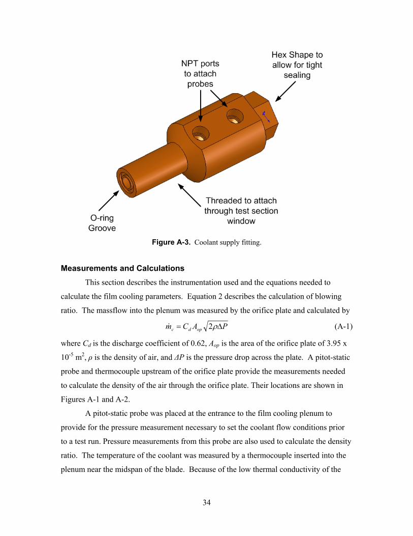
A fitting was designed to provide air through the test section window into the plenum.
The fitting, shown in Figure A-3, connects to copper tubing on one end and uses an o-
ring to provide for a face seal against the blade. This provides air to the plenum without
leakage.
The control valve is a proportional type control with the valve opening
proportionally to the amount of air pressure that is applied to it. Shop air provides the
pressure needed to open the valve. A signal pressure is supplied by an electro-pneumatic
converter that converts a voltage input to a proportional pressure output. Increasing the
signal pressure will increase the amount of air that is allowed to pass through the valve.
Air is supplied to the plenum at a constant pressure throughout the run. Before
the tunnel is operated, the supply of air to the plenum is set with the control valve. A
readout of the plenum pressure, measured with a pitot-static probe, is monitored while
adjusting the control valve. When the desired pressure is reached, the tunnel control is
started. This provides a constant blowing ratio as shown in Figure 8.
33
Figure A-1. Film cooling system schematic. Locations of pressure and temperature measurements are indicated.
Figure A-2. Photograph of film cooling supply.
34
Figure A-3. Coolant supply fitting.
Measurements and Calculations
This section describes the instrumentation used and the equations needed to
calculate the film cooling parameters. Equation 2 describes the calculation of blowing
ratio. The massflow into the plenum was measured by the orifice plate and calculated by
PACm opdc Δ= ρ2& (A-1)
where Cd is the discharge coefficient of 0.62, Aop is the area of the orifice plate of 3.95 x
10-5 m2, ρ is the density of air, and ΔP is the pressure drop across the plate. A pitot-static
probe and thermocouple upstream of the orifice plate provide the measurements needed
to calculate the density of the air through the orifice plate. Their locations are shown in
Figures A-1 and A-2.
A pitot-static probe was placed at the entrance to the film cooling plenum to
provide for the pressure measurement necessary to set the coolant flow conditions prior
to a test run. Pressure measurements from this probe are also used to calculate the density
ratio. The temperature of the coolant was measured by a thermocouple inserted into the
plenum near the midspan of the blade. Because of the low thermal conductivity of the
35
Macor blade, it was assumed that the temperature of the plenum was the same as the
temperature of the coolant as it exited the coolant holes.
Checklists were used for each run to record the parameters used and provide for
consistent operation. These were authored by Bolchoz and are contained in this
appendix. A pre-run checklist was used to prepare for each day of tests and a tunnel run
checklist was used to set and record the conditions of each run.
After 1 hour, set air bottle pressure to 100<P(psi)<120.
Disconnect trigger for calibration.
Calibrate PSI 8400.
After calibration, switch air to tunnel control valve
(P=25psi).
Reconnect trigger
Film Cooling System
Close off open valves on film-cooling tank and start
compressor.
Go outside and make sure that compressor is on, dryer is
on, and ball valve exiting compressor is open.
Charge tank to 120 psi and turn off compressor.
Turn on shop air to control valve.
Inspect cooling instrumentation and ensure that thermocouples/pitot probes are in correct positions and
that everything is connected with desired flow path set.
Heater
Open heater loop, and turn on fan/heater.
Heat to 600°F on bottom display, and then allow heater to
cool to 300°F.
Turn heater on again and repeat process until target of
232°F is reached on top display.
Instrumentation
Turn on DAQ and MKS transducers and zero MKS.
Measure pre-run resistances of TFG’s and record in input
file.
Supply 10VDC(± 3mV) to Wheatstone bridge circuit.
Measure with multimeter and record voltage in
input file.
Measure Wheatstone bridge output for each gage and use
potentiometers to zero the gage (± 0.005 mV).
Tunnel
Start tunnel compressor and turn on panel/tunnel computer.
Get atmospheric pressure and enter into input file on
computer and tunnel control software.
Set tunnel objective pressure in control software.
Ensure that all clamps on tunnel windows are secure
Place safety shields in front of tunnel windows.
Record the overall purpose of the day’s experiments in the
tunnel run log.
37
Tunnel Run with Cooling Checklist
Test Objective: ____________________________________________
Before Run:
Open heater loop. Cool blade to room temperature.
Cooling System
Ensure that cooling tank is charged to 100 psi and that compressor is off. Ensure that cooling is routed through chiller. Set voltage supply to 0V. Open manual and solenoid valves.
Heater
Ensure that heater loop is open with 2 valves. Heat copper tubes to 232°C. Turn heaters off, but keep fan on.
Tunnel
Make sure that tunnel is set to run from outside Set air bottle pressure to 25 psi for tunnel control valve. Charge tunnel tank to 140 psi.
DAQ
Make sure that PSI is calibrated and acquiring. Have appropriate DAQ .vi ready to record.
Running:
Pour _____ inches of nitrogen into the cooler. Start stopwatch and slowly increase voltage, monitoring plenum total pressure
reading on MKS for initial pressure spike; then set the pressure to appropriate value ______Volts.
At _____ seconds, cooling operator should open green heater loop valve while another operator shuts off fan.
At _____ seconds, the other operator should open the downstream heater valve. At this point both operators leave room, and the tunnel/DAQ should be started.
After run, record test information in log.
Notes:
38
Appendix B: Double-sided Gage Installation Gage Mounting. Double-sided gages were constructed from platinum thin film
gages manufactured by the Air Force Research Laboratories and 0.5 mil thin foil
thermocouples manufactured by RDF corporation. The platinum thin film gages are laid
with their adhesive side up as shown in Figure B-1. The paper backing is removed from
the adhesive a few gages at a time. A thin foil thermocouple is then mounted to adhesive
backing of the platinum thin film gages. The sensing junction of the thermocouple is
aligned to the midspan of the platinum portion of the thin film gage with the aid of a pair
of tweezers. The thermocouple leads are then extended across the adhesive portion of the
gage sheet. The sheet is placed over a lined substrate to provide guidance so that the
thermocouple leads can be arranged parallel with each other. Figure B-1 shows a gap
where two platinum gages were left without a backwall thermocouple. This area of the
gage sheet corresponds to the cooling hole row locations on the leading edge of the blade.
Figure B-1. Installation of thermocouples to Pt thin film gages(L). The attachment of the gage sheet to the blade(R).
Once the entire sheet of platinum thin film gages had been instrumented with
backwall thermocouples, the sheet was applied to the showerhead film cooled blade. The
midspan location of the blade was marked and the gages were aligned starting with the
“empty” gages at the leading edge of the blade. The sheet was slowly wrapped around
the blade on the suction side. Care was taken to apply the sheet slowly and to apply
pressure in a rubbing fashion towards the blade endwalls away from the midspan to
prevent air from being trapped beneath the gage sheet. After the suction side gages had
39
been successfully installed, the blade was rotated in its stand and the process was
repeated on the pressure side of the blade.
Film Cooling Holes. Once the gage sheet had been installed, the cooling holes
had to be placed in the gage sheet. Holes had previously drilled through the surface of
the blade into the cooling plenum, but were covered up when applying the gage sheet.
On one half of the span of the blade, the copper leads of the thin film gages covered up
the cooling holes. This copper lead was carefully scraped away using an X-ACTO®
blade. This process was able to be completed without roughening the kapton surface.
A soldering iron was equipped with a thin, conical tip and heated to a setting of
~700ºF. The soldering iron was aligned to the spanwise angle of the cooling hole. Then,
the heated soldering tip was used to pierce a hole in the kapton. A heated soldering iron
was used because it produced a hole while preventing the kapton from ripping. A drill bit
the same diameter as the cooling hole was placed in a pen vise and then used to clear the
kapton material from the cooling hole. If a “hanging-chad” of kapton material was left in
the cooling hole, the back end of the drill bit(the part normally inserted into the drill
chuck) was used to cut and push the kapton through the hole into the plenum. The kapton
material was cleared from the plenum and each cooling hole was visually inspected to
insure that there was no blockage.
Lead Wires. Lead wires were soldered to the platinum thin film gage following
the procedure outlined in Carullo[18]. The leads were covered with JB weld to
physically secure them and protect them from the tunnel flow. The blade was then placed
inside an oven for calibration of the thin film gages. The calibration procedure is
discussed by Cress [20]. After calibration, the blade was mounted to the clear, Lexan test
section window. A layer of silicon caulk was applied over the JB weld to secure the
blade to the window and to provide for a smooth surface for the flow to go over.
An aluminum “insert” was attached to the thermocouple side of the blade. This
insert allowed for the blade to be removed from the test section without disturbing the
gage configuration. An image of this setup is provided in B-2. The thermocouple leads
extended off the span of the blade in the opposite spanwise direction as the thin film
gages. Thermocouple wires were inserted through holes in the “insert” and soldered to
the leads. Soldered leads were covered with a layer of silicon caulk to protect them from
40
the elements and seal the tunnel test section. Figure B-3 shows the gages mounted with
the lead wires soldered and shows the instrumented blade installed into the cascade.
Figure B-2. Blade with lexan window and aluminum insert.
Figure B-3. Photographs of installed test hardware. Lead wires attached to thin film gages and thermocouples(L). Instrumented blade installed to test section with film cooling supply shown(R).
41
Appendix C: Material Properties Calibration This appendix describes the process used to calibrate for the material properties of
the double-sided gage used in this work. Figure C-1 shows an expanded schematic of
this gage.
Figure C-1. Expanded schematic of the double-sided gage.
The heat flux the blade experiences during a typical tunnel run depends on
location of the blade but can range from 12 kW/m2 to 30 kW/m2. A step input of heat
flux was imposed on the gage by a laser, and the response time of the gage was
determined to be about 30 ms. This response time was also seen in a double-sided gage
described by Ewing et al.[C-1]. This heat flux gage measures temperatures on either side
of a kapton and adhesive layer that is around 70 μm thick. Since this gage measures a
high heat flux over a very thin layer and possesses a fast response time, it can be assumed
that the temperature profile through the gage is linear. The heat flux through the gage
can be described by
)(" bw TTlkq −= (C-1)
where Tw is the platinum thin film gage temperature, Tb, is the backwall thermocouple
temperature, and k/l is the thermal conductivity divided by the gage thickness.
Cress [20] developed a one-dimensional finite difference code to find the heat
flux into the blade using a platinum thin film gage as the surface temperature. This code
42
was adapted to solve for the heat flux into the macor blade using the backwall
thermocouple, Tb, as the input. With the heat flux as a known and assuming that the heat
flux into the gage is the same as the heat flux into the blade, Equation C-1 can be
arranged as
)(
"
bw
FD
TTq
lk
−= (C-2)
where "FDq is the heat flux determined from the finite difference code.
The finite difference code is valid at locations on the blade away from the film
cooling plenum during a tunnel run where film cooling is not introduced. Three heated
tunnel runs at Me=0.78, Tu=2%, and no film cooling were used to provide the conditions
necessary for this calibration. Three gage locations where the finite difference code was
valid were analyzed to determine the k/l of the kapton and macor.
For three gages over three tunnel runs the k/l value was determined to be 1240 ±
90 W/m2-K using the 95% confidence interval. Bias error was found using Moffat’s [21]
small perturbation method and precision error was found from gage to gage and run to
run repeatability. Assuming that the adhesive layer does not change its thickness due to
mounting, the conductivity of the kapton used in the current research was found to be
0.09 ± 0.006 W/m-K. Once the material properties of these gages were calibrated during
an uncooled tunnel run, they could be used in a film cooled environment.
References [C-1] Ewing, Jerrod, 2006, “Development of a Direct-Measurement Thin film Heat Flux Array,” Master’s Thesis, Virginia Tech
43
Appendix D: Uncertainty Analysis This appendix describes how the uncertainty of of h and η were determined.
Heat transfer coefficient was determined from the slope of the line fit shown in Figure D-
1. Each data point has an uncertainty in its x location and y location. This uncertainty
was determined within the 95% confidence interval using Moffat’s [21] small
perturbation method. The linear regression equation is applied to the set of data points
and the equation of the line is calculated.
Figure D-1. Description of Uncertainty
Brown et al.’s [22] method was used to determine the uncertainty of the line fit
through the data. The bias error in the x and y direction determined from the small
perturbation method were used as an input to Brown et al.’s [22] analysis procedure.
Covariance was assumed to be negligible. The uncertainty in the slope and x-intercept
determined from this procedure is the uncertainty in h and η, respectively.
The standard linear regression equation assumes that all error is contained within
the y-axis data. This happens to be a good assumption in this case because the magnitude
of error in the y-axis is much greater than that in the x-axis. Reed [D-1] describes a
method used to fit a line through data with error in both the x and y axis. To further
validate that a fit method assuming only y-axis uncertainty was appropriate for this work,
Reed’s[D-1] method was used on sample data sets and slope and intercept were
44
compared to those found using the standard fit method. The differences in the results of
the two methods was determined to be negligible. The standard regression equation was
used in this work because it provided the same results as York’s method without the need
for iteration.
Uncertainty values for intermediate and final results are shown in Table D-1.
Uncertainties in Me, DR, and BR were determined with Moffat’s [21] small perturbation
method within the 95% confidence interval. Precision uncertainty for k/l was determined
using run to run and gage to gage repeatability. Samples of data plotted with the
uncertainty band are provided for Nusselt number and Effectiveness in Figures D-2 and
D-3, respectively.
Table D-1. Uncertainty Values
Value Uncertainty (± Percentage)
h 10
η 20 "redqΔ 17
k/l 7
Me 1.3
DR 0.4
BR 1.4
45
0
500
1000
1500
2000
2500
-1.2 -0.8 -0.4 0.0 0.4 0.8 1.2 1.6
s/C
Nu
-100 -80 -60 -40 -20 0 20 40 60 80 100 120s/d
BR = 1.0
BR = 1.5
Uncooled, Carullo et al. [17]
Cooling Hole Row
PS SS
Figure D-2. Nusselt number Distribution with uncertainty included. This is Figure 9 plotted with error included.
0.00
0.10
0.20
0.30
0.40
0.50
0.60
0.70
-1.2 -0.8 -0.4 0.0 0.4 0.8 1.2 1.6s/C
η
-100 -80 -60 -40 -20 0 20 40 60 80 100 120s/d
BR = 1.0
BR = 1.5
Cooling Hole Row
Zhang et al.[16] -BR=0.85, DR=1, Tu=6%
PS SS
Figure D-3. Effectiveness Distribution with uncertainty included. This is Figure 11 plotted with error included.
References [D-1] Reed, B.C., “Linear least-squares fits with errors in both coordinates,” American Journal of Physics, Vol. 57, No. 7, 1989, pp. 642-646
46
Appendix E: Tabulated Results This appendix contains results previously presented in graphical form as tabulated
Appendix F: Data Reduction Code This appendix contains the MATlab mfile that was used to reduce the data. Data
was saved in four files: input file, NI file, NI initial value file, and PSI file. The input file
contained all of the data related to that day of testing including pre run resistances, thin
film calibration constants, atmospheric pressure. It also included gage data including
location, material properties, and local Mach number. All pressures were recorded by the
PSI 8400 (PSI) system and were in the PSI file. Two files were recorded using the
National Instruments AT-MIO-16XE-50 system(NI). A file containing the initial
temperatures was recorded prior to starting any coolant. Then during testing, the NI
system recorded all voltages and temperatures.
This mfile reads in all of the data files and computes all quantities of interest in
this work. An option for saving the reduced data in an excel file is given. Included in
this mfile are the codes needed to make plots of interest.
Code: clear all close all clc %format long global N fs %Read in data from 4 files, a daily input file, PSI 8400 output, and %NI daq system %temperature and voltage history in NI data and NI initial value file, %pressures in PSI data %%%%%%%%%%file names p1='z:\Solar_Research\Film_Cooled\Tunnel Test\Final Blade\12_Turbulence\Mach 0_80\BR_1\'; date='04-19-07'; r1='Run'; r2='_'; r3='4';%%%%%%%%Run # Run=[r1 r2 r3]; Rund=[r1 ' ' r3];%title for plots NI='\NI_'; PSI='\PSI_'; p2='.lvm'; NI_file=[p1 date NI Run p2]; PSI_file=[p1 date PSI Run]; reduce='_reduced_final'; init='_init'; p3='.xls'; slash='\'; IN='Input '; savename=[p1 date slash Run reduce p3];%name for saved excel results file input_name=[p1 date slash IN date p3]; init_file=[p1 date NI Run init p2]; fs=1000;% NI sampling rate(Hz) psi_fs=20;%psi sampling rate(Hz) %%%%%%%%%input files%%%%%%%%%%%% NI_data_prefilt=dlmread(NI_file); init_data=dlmread(init_file); PSI_data=dlmread(PSI_file,'\t',1,0); input=xlsread(input_name,'input','B2:I17');
49
%%%%%%%%%%%%%%%%%%%%%%%%%%%%%%%%%%%%%%%%%%%% name for plots/saving gagename=['Gage 01';'Gage 02';'Gage 03';'Gage 04';... 'Gage 05';'Gage 06';'Gage 07';'Gage 08';'Gage 09';'Gage 10';... 'Gage 11';'Gage 12';'Gage 13';'Gage 14';'Gage 15';'Gage 16']; gagename2=[1:1:16]; gagename3=[1,1,2,2,3,3,4,4,5,5,6,6,7,7,8,8,9,9,10,10,11,11,12,12,13,13,... 14,14,15,15,16,16]; numberofgage=16; Vbridgesupply=input(1,7);%voltage supplied to wheatstone bridge Patm_bar=input(1,8); %atmospheric pressure in bars Patm=Patm_bar/6894.75;%convert to psi r=0.892;%recovery factor for turbulent flow Kelvin_con=273.15;%convert deg C to Kelvins %name input data for a=1:numberofgage k_l(a)=input(a,1); %k/l W/m^2-K Kcalib(a)=input(a,2);%TFG calibration slope ohm/C R20(a)=input(a,3);%TFG Resistance at 20 deg C x_c(a)=input(a,4);%x/c location of gage M_loc(a)=input(a,5);%local Mach number at gage location Rprun(a)=input(a,6);%pre-run resistance of TFG gage end %filter NI data aba=size(NI_data_prefilt);%number of data columns [d,e] = butter(5,30/500);%define filter for i = 2:aba(2)%every NI column except time NI_data(:,i) = filtfilt(d,e,NI_data_prefilt(:,i)); end %time data time=NI_data_prefilt(:,1); time=time-time(1);%convert b/c sometimes DAQ doesn't start time at zero N=length(NI_data); Npsi=length(PSI_data); %name and sort NI data for a=1:numberofgage %NI Column structure time, TFG backwalls,tfreetot,TFG voltages for b=1:N T_backwall(b,a)=NI_data(b,a+1);%deg C T_free_tot_prelag(b)=NI_data(b,2+numberofgage);%deg C TFG_volt(b,a)=NI_data(b,numberofgage+a+2);%Volt Ttot_plen_slide_NI(b)=NI_data(b,2*numberofgage+4);%sampled from end end %%%%%%%%%%%%name and sort initial value file%%%%%%%%%%%%%%%%%% for a=1:numberofgage %NI Column structure time, TFG backwalls,tfreetot,TFG voltages for b=1:length(init_data) T_backwall_initial(b,a)=init_data(b,a+1);%deg C TFG_volt_initial(b,a)=init_data(b,numberofgage+a+2);%volt end end for a=1:numberofgage T_TFG_init(a)=mean(T_backwall_initial(:,a)); TFG_volt_init(a)=mean(TFG_volt_initial(:,a)); end %%%%%%%%%%%%%%%%%%%%%%%%%%%%%%%%%%%%%%%%%%%%%%%%%%%%%%%%%%%%% lagTC=0.1;%lag the freestream TC measurement --located upstream T_free_tot=zeros(1,N); T_lag=T_free_tot_prelag(lagTC*fs:N); for b=1:length(T_lag) T_free_tot(b)=T_free_tot(b)+T_lag(b); end %name PSI data (all data is in units of PSI) ttpsi=0; lead_psi=0.6;%seconds to lead psi data--psi trigger takes time to start psi_count=psi_fs*lead_psi; for c=1:Npsi Ptot_up(c)=PSI_data(psi_count,1); Pstat_free_up(c)=PSI_data(psi_count,2); Pstat_up_1(c)=PSI_data(psi_count,3); Pstat_up_2(c)=PSI_data(psi_count,4);
50
Pstat_up_3(c)=PSI_data(psi_count,5); Pstat_down_1(c)=PSI_data(psi_count,6); Pstat_down_2(c)=PSI_data(psi_count,7); Pstat_down_3(c)=PSI_data(psi_count,8); Pstat_down_4(c)=PSI_data(psi_count,9); Orifice_up(c)=PSI_data(psi_count,10); Orifice_down(c)=PSI_data(psi_count,11); Orifice_up_Ptot(c)=PSI_data(psi_count,12); Orifice_up_Pstat(c)=PSI_data(psi_count,13); Ptot_plen(c)=PSI_data(psi_count,14); Pstat_plen(c)=PSI_data(psi_count,15); Pstat_down_avg(c)=(Pstat_down_1(c)+Pstat_down_2(c)+Pstat_down_3(c)... +Pstat_down_4(c))/4; Pr_up(c)=(Ptot_up(c)+Patm)/(Pstat_free_up(c)+Patm); Pr_down(c)=(Ptot_up(c)+Patm)/(Pstat_down_avg(c)+Patm); M_up(c)=sqrt(2/0.4*(Pr_up(c)^(.4/1.4)-1)); M_down(c)=sqrt(2/0.4*(Pr_down(c)^(.4/1.4)-1)); Orifice_dP(c)=Orifice_up(c)-Orifice_down(c); time_psi(c)=ttpsi; ttpsi=ttpsi+1/psi_fs;%make a time vector the same length as the psi data if psi_count<Npsi psi_count=psi_count+1; else psi_count=600; end end %%%%find tunnel start time pp=1; for n=1:Npsi; if Ptot_up(n)>0.007 break end pp=pp+1; end tunnel_start_count=pp; tunnel_start=pp/psi_fs;%tunnel start time in seconds %for blowing calculations, must oversample data b/c NI samples MKS %transducers at a very high rate z=1; for a=1:50:N Tfree_tot_blow(z)=T_free_tot(a);%tunnel tot Ttot_plen_fit(z)=NI_data(a,2*numberofgage+3);%Ttot plenum on fitting Ttot_plen_slide(z)=NI_data(a,2*numberofgage+4);%sliding plenum Ttot Orifice_up_Ttot(z)=NI_data(a,2*numberofgage+5);%Ttot line-upstream of orifice z=z+1; end A_holes=47*pi/4*(0.033*2.54/100)^2;%area of cooling holes m^2 discharge_coef=0.62;%discharge coefficient of orifice plate bore_area=pi/4*(0.2795*2.54/100)^2;%m^2 area of orifice plate %%%calculate blowing conditions for a=1:Npsi Pr_plen(a)=(Ptot_plen(a)+Patm)/(Pstat_plen(a)+Patm); M_plen(a)=sqrt(2/0.4*(Pr_plen(a)^(.4/1.4)-1)); Tstat_free(a)=(Tfree_tot_blow(a)+Kelvin_con)/(1+0.2*M_up(a)^2);%K Tstat_free_down(a)=(Tfree_tot_blow(a)+Kelvin_con)/(1+0.2*M_down(a)^2);%downstream stat temp K rho_stat_free(a)=(Pstat_free_up(a)+Patm)*6894.75/(287*Tstat_free(a));%upstream density kg/m^3 rho_stat_free_down(a)=(Pstat_down_avg(a)+Patm)*6894.75/(287*Tstat_free_down(a));%downstream density kg/m^3 rhou_free(a)=rho_stat_free(a)*M_up(a)*sqrt(1.4*287*Tstat_free(a));%kg/m^2-s pr_orf_up(a)=(Orifice_up_Pstat(a)+Patm)/(Orifice_up_Ptot(a)+Patm); Tstat_line(a)=(Orifice_up_Ttot(a)+Kelvin_con)*pr_orf_up(a)^(0.4/1.4); %upstream of orifice plate(K) rho_line(a)=(Orifice_up_Pstat(a)+Patm)*6894.75/(287*Tstat_line(a)); mdot_cool(a)=discharge_coef*bore_area*sqrt(2*rho_line(a)*Orifice_dP(a)*6894.75);%kg/s Tstat_plen(a)=(Ttot_plen_slide(a)+Kelvin_con)/(1+0.2*M_plen(a)^2);%K --using Tprobe slide into plenum rho_plen(a)=(Pstat_plen(a)+Patm)*6894.75/(287*Tstat_plen(a));%kg/m^2
51
mu(a)=0.00001716*((Tfree_tot_blow(a)+Kelvin_con)/273.16)^1.5*... (383.716/((Tfree_tot_blow(a)+Kelvin_con)+110.556)); vel_down(a)=M_down(a)*sqrt(1.4*287*Tstat_free_down(a)); Re_down(a)=rho_stat_free_down(a)*vel_down(a)*(2.7505*2.54/100)/mu(a); DR(a)=rho_plen(a)/rho_stat_free(a);%Density Ratio PR(a)=(Ptot_plen(a)+Patm)/(Ptot_up(a)+Patm);%Pressure Ratio BR(a)=(mdot_cool(a)/A_holes)/rhou_free(a);%Blowing Ratio end clear NI_data NI_data_prefilt PSI_data M_down_t=M_down';%transpose matrix for saving time_psi_t=time_psi'; %%%%HTC Data reduction HTC_reduce_time=3; reducestart=tunnel_start+3; reduceend=reducestart+HTC_reduce_time; %draw lines to show where reducing data starts and ends red_start_x=[reducestart,reducestart]; red_end_x=[reduceend,reduceend]; red_start_y=[0,40e3]; red_end_y=[0,40e3]; Mach_redtime=M_down(1,round(reducestart*psi_fs):round(reduceend*psi_fs)); BR_redtime=BR(1,round(reducestart*psi_fs):round(reduceend*psi_fs)); DR_redtime=DR(1,round(reducestart*psi_fs):round(reduceend*psi_fs)); Re_redtime=Re_down(1,round(reducestart*psi_fs):round(reduceend*psi_fs)); Mex_avg=mean(Mach_redtime); BR_avg=mean(BR_redtime); DR_avg=mean(DR_redtime); Re_avg=mean(Re_redtime); Mstring=['Mex= ' num2str(Mex_avg)]; BRstring=['BR= ' num2str(BR_avg)]; DRstring=['DR= ' num2str(DR_avg)]; %Plot Mach Number and BR--shows data reduction window figure hold on title(Rund) hl1=line(time_psi,M_down,'Color','b'); axis([tunnel_start 30 0 1.1]) xlabel('Time,(s)') ylabel('Mach, Exit') line(red_start_x,red_start_y) line(red_end_x,red_end_y) ax1=gca; set(ax1,'XColor','b','Ycolor','b') ax2=axes('Position',get(ax1,'Position'),'YAxisLocation',... 'right','Color','none','XColor','k','YColor','k'); hl2=line(time_psi,BR,'Color','k','Parent',ax2); axis([tunnel_start 30 0 2]) ylabel('Blowing Ratio') text(20,0.5,{Mstring,BRstring,DRstring},'EdgeColor','black') hold off savedata=0 %%%%%%%%%%%%%%%%Convert TFG voltages to temperature Rline=0.145;%resistance of cord Rs=10000;%series resistance of bridge for a=1:numberofgage TFG_volt(:,a)=TFG_volt(:,a)-TFG_volt_init(a);%offset TFG voltage to zero %correct the calibration for day to day variation Kcor(a)=Kcalib(a)*(Rprun(a)-Rline)/R20(a); Rt(a)=Rline+Rs+Rprun(a); for j=1:N del_T_Pt_TFG(j,a)=TFG_volt(j,a)*Rt(a)/(Kcor(a)*... (Rs/Rt(a)*Vbridgesupply-TFG_volt(j,a))); T_Pt_TFG(j,a)=T_TFG_init(a)+del_T_Pt_TFG(j,a);%deg C %TFG finds change in temp, so must add initial temp q_to_blade(j,a)=k_l(a)*(T_Pt_TFG(j,a)-T_backwall(j,a)); %local Taw for uncooled (Kelvins) Trec(j,a)=(T_free_tot(j)+Kelvin_con)*... ((1+r*0.2*M_loc(a)^2)/(1+.2*M_loc(a)^2)); end end
52
%%%%%%%%%%%%%%%calculations of h and eta for a=1:numberofgage ggg=1; %reduce HTC for set time after tunnel start for j=round(reducestart*fs):round(reduceend*fs) yax(ggg,a)=q_to_blade(j,a)/... (Trec(j,a)-(Ttot_plen_slide_NI(j)+Kelvin_con)); xax(ggg,a)=(Trec(j,a)-(T_Pt_TFG(j,a)+Kelvin_con))... /(Trec(j,a)-(Ttot_plen_slide_NI(j)+Kelvin_con)); ggg=1+ggg; end lineeq_o=polyfit(xax(:,a),yax(:,a),1); lineeq(1,a)=lineeq_o(1); lineeq(2,a)=lineeq_o(2); R_coef=corrcoef(xax(:,a),yax(:,a)); R_squared(1,a)=R_coef(2,1)^2; evallinex(:,a)=(linspace((min(xax(:,a))-0.01),(max(xax(:,a))+0.01),10))'; evalliney(:,a)=(lineeq(1,a)*evallinex(:,a)+lineeq(2,a)); eta(1,a)=-lineeq(2,a)/lineeq(1,a); HTC_avg(1,a)=lineeq(1,a); end xtextloc=1.04*mean(xax); ytextloc=0.96*mean(yax); %%%reduce HTC and Taw time history--assuming eta is constant for entire run %%%should only analyze results during time eta is calculated from. for a=1:numberofgage for b=1:N %Taw (K) --assuming eta=k for run Taw(b,a)=eta(1,a)*... (Ttot_plen_slide_NI(b)+Kelvin_con-Trec(b,a))+Trec(b,a); %HTC time history W/m^2-K HTC(b,a)=q_to_blade(b,a)/(Taw(b,a)-(T_Pt_TFG(b,a)+Kelvin_con)); end end %%%%%%%%%%%%%SAVE OUTPUT%%%%%%%%%%%%%%%%%%%%%%%%% %stop reduction and look at conditions to see if you want to save the data %check out reduction window and see if flow conditions are steady %if you choose, data will be saved in an excel file organized into %separate tabs of data keyboard if savedata==1 Nu_avg=HTC_avg*(2.7505*2.54/100)/0.03; oddcount=1; evencount=2; for a=1:numberofgage axisdata(:,oddcount)=xax(:,a); axisdata(:,evencount)=yax(:,a); oddcount=oddcount+2; evencount=evencount+2; end xlswrite(savename,gagename3,'Average Values','B1') xlswrite(savename,axisdata,'axisdata','B2') avgarray(1,:)=HTC_avg(1,:); avgarray(2,:)=eta(1,:); avgarray(3,:)=R_squared(1,:); avgarray(5,1)=Mex_avg; avgarray(6,1)=BR_avg; avgarray(7,1)=DR_avg; avgarray(9,1)=reducestart; avgarray(10,1)=reduceend; avgarray(12,1)=tunnel_start; avgarray(14,:)=T_TFG_init(1,:); avgarray(15,:)=TFG_volt_init(1,:); avgarray(17,:)=Nu_avg(1,:); avgarray(18,1)=Re_avg; xlswrite(savename,gagename2,'Average Values','B1') xlswrite(savename,avgarray,'Average Values','B2') savearray_flow(:,1)=time_psi_t; savearray_flow(:,2)=M_down_t;
53
savearray_flow(:,3)=Ptot_up'; savearray_flow(:,4)=Pstat_free_up'; savearray_flow(:,5)=Pstat_up_1'; savearray_flow(:,6)=Pstat_up_2'; savearray_flow(:,7)=Pstat_up_3'; savearray_flow(:,8)=Pstat_down_1'; savearray_flow(:,9)=Pstat_down_2'; savearray_flow(:,10)=Pstat_down_3'; savearray_flow(:,11)=Pstat_down_4'; savearray_flow(:,12)=Tfree_tot_blow'; xlswrite(savename,savearray_flow,'Flow History','A2') T_free_tot_s=T_free_tot(1,1:N); T_free_tot=T_free_tot'; savearray_blowing(:,1)=time_psi_t(:,1); savearray_blowing(:,2)=BR'; savearray_blowing(:,3)=DR'; savearray_blowing(:,4)=PR'; savearray_blowing(:,5)=M_plen'; savearray_blowing(:,6)=Tstat_free'; savearray_blowing(:,7)=rho_stat_free'; savearray_blowing(:,8)=mdot_cool'; savearray_blowing(:,9)=Tstat_plen'; savearray_blowing(:,10)=Ptot_plen'; savearray_blowing(:,11)=Pstat_plen'; savearray_blowing(:,12)=Ttot_plen_fit'; savearray_blowing(:,13)=Ttot_plen_slide'; xlswrite(savename,savearray_blowing,'Blowing','A2') %oversample data to save time_s=time(1:10:N,1); for a=1:numberofgage yyy=1; for zzz=1:10:N T_backwall_s(yyy,a)=T_backwall(zzz,a); T_Pt_TFG_s(yyy,a)=T_Pt_TFG(zzz,a); HTC_s(yyy,a)=HTC(zzz,a); q_to_blade_s(yyy,a)=q_to_blade(zzz,a); Taw_s(yyy,a)=Taw(zzz,a); Trec_s(yyy,a)=Trec(zzz,a); Tcool_s(yyy)=Ttot_plen_slide_NI(zzz); yyy=1+yyy; end end %heat flux data xlswrite(savename,gagename2,'Tbackwall','B1') xlswrite(savename,T_backwall_s,'Tbackwall','B2') xlswrite(savename,gagename2,'T Pt TFG','B1') xlswrite(savename,T_Pt_TFG_s,'T Pt TFG','B2') xlswrite(savename,gagename2,'HTC','B1') xlswrite(savename,HTC_s,'HTC','B2') xlswrite(savename,gagename2,'Heat Flux','B1') xlswrite(savename,q_to_blade_s,'Heat Flux','B2') xlswrite(savename,gagename2,'Taw','B1') xlswrite(savename,Taw_s,'Taw','B2') xlswrite(savename,gagename2,'Trec','B1') xlswrite(savename,Trec_s,'Trec','B2') xlswrite(savename,T_free_tot_s','Ttot free','B2') xlswrite(savename,Tcool_s','Tcool','B2') end tunnel_run_time=tunnel_start:psi_fs:30; %%%%%%%%%%%%%%%%%%%PLOTS%%%%%%%%%%%%%%%%%%% figure plot(x_c,HTC_avg,'o') xlabel('x/c') ylabel('HTC, (W/m^2-K)') figure plot(x_c,eta,'o') xlabel('x/c') ylabel('\eta') figure plot(x_c,del_q_r,'o')
54
xlabel('x/c') ylabel('\Delta''q_r, (W/m^2)') %Plot Mach Number and DR figure hold on title(Rund) hl1=line(time_psi,M_down,'Color','b'); axis([tunnel_start 30 0 1]) xlabel('Time,(s)') ylabel('Mach, Exit') line(red_start_x,red_start_y) line(red_end_x,red_end_y) ax1=gca; set(ax1,'XColor','b','Ycolor','b') ax2=axes('Position',get(ax1,'Position'),'YAxisLocation',... 'right','Color','none','XColor','k','YColor','k'); hl2=line(time_psi,DR,'Color','k','Parent',ax2); axis([tunnel_start 30 0 2]) ylabel('Density Ratio') text(20,1,{Mstring,BRstring,DRstring},'EdgeColor','black') hold off %Mach figure hold on xlabel('Time (s)') line(red_start_x,red_start_y) line(red_end_x,red_end_y) ylabel('Mexit') axis([tunnel_start,30,0,1]) plot(time_psi,M_down) hold off % BR figure hold on xlabel('Time (s)') % ylabel('Blowing Ratio') line(red_start_x,red_start_y) line(red_end_x,red_end_y) % axis([tunnel_start,30,0,3]) % plot(time_psi,BR) hold off % PR figure hold on xlabel('Time (s)') ylabel('Pressure Ratio') line(red_start_x,red_start_y) line(red_end_x,red_end_y) axis([tunnel_start,30,0,2]) plot(time_psi,PR) hold off % DR figure hold on xlabel('Time (s)') ylabel('Density Ratio') axis([tunnel_start,30,0,3]) line(red_start_x,red_start_y) line(red_end_x,red_end_y) % plot(time_psi,DR) hold off %temperature plots figure hold on title({Rund}) axis([0 30 200 400]) plot(time,(T_free_tot+Kelvin_con),time,... Taw(:,a),time,Trec(:,a),time,(Ttot_plen_slide_NI+Kelvin_con)) legend('Ttot free','Taw','Trec','Tcoolant') line(red_start_x,red_start_y) line(red_end_x,red_end_y)
55
xlabel('Time (s)') ylabel('Temperature (K)') hold off %%%%%%%%%%%%%subplots of all gage signals%%%%%%%%%%%%%% figure for a=1:numberofgage/2 subplot(4,2,a);plot(time,T_Pt_TFG(:,a),time,T_backwall(:,a)) xlabel('Time (s)') ylabel('T,(C)') title(gagename(a,:)) end figure for a=numberofgage/2+1:numberofgage subplot(4,2,a-8);plot(time,T_Pt_TFG(:,a),time,T_backwall(:,a)) xlabel('Time (s)') ylabel('T,(C)') title(gagename(a,:)) end figure for a=1:numberofgage/2 subplot(4,2,a);plot(time,(T_Pt_TFG(:,a)-T_backwall(:,a))) xlabel('Time (s)') ylabel('\Delta T') title(gagename(a,:)) end figure for a=numberofgage/2+1:numberofgage subplot(4,2,a-8);plot(time,(T_Pt_TFG(:,a)-T_backwall(:,a))) xlabel('Time (s)') ylabel('\Delta T') title(gagename(a,:)) end figure for a=1:numberofgage/2 subplot(4,2,a);plot(time,HTC(:,a)) line(red_start_x,red_start_y) line(red_end_x,red_end_y) axis([0 20 0 1000]) xlabel('Time (s)') ylabel('h') title(gagename(a,:)) end figure for a=numberofgage/2+1:numberofgage subplot(4,2,a-8);plot(time,HTC(:,a)) line(red_start_x,red_start_y) line(red_end_x,red_end_y) axis([0 20 0 1000]) xlabel('Time (s)') ylabel('h') title(gagename(a,:)) end %%%%plots of data reduction line fit method for a=1:numberofgage hstring=['h= ' num2str(round(lineeq(1,a))) ' W/m^2-K']; etastring=['\eta= ' num2str(eta(1,a))]; regstring=['R^2= ' num2str(R_squared(1,a))]; figure
56
hold on title({Rund,gagename(a,:)}) xlabel('(Tr-Tw)/(Tr-Tc)') ylabel('q/(Tr-Tc)') plot(xax(:,a),yax(:,a),'.','MarkerSize',4) plot(evallinex(:,a),evalliney(:,a),'-k') text(xtextloc(a),ytextloc(a),... {hstring,etastring,regstring},'EdgeColor','black') hold off slope(1,a)=lineeq(1,a); yint(1,a)=lineeq(2,a); end figure for a=1:numberofgage/2 subplot(4,2,a);plot(time,TFG_volt(:,a)) xlabel('Time (s)') ylabel('Volt') title(gagename(a,:)) end figure for a=numberofgage/2+1:numberofgage subplot(4,2,a-8);plot(time,TFG_volt(:,a)) xlabel('Time (s)') ylabel('Volt') title(gagename(a,:)) end figure for a=1:numberofgage/2 subplot(4,2,a);plot(time,phi(:,a)) xlabel('Time (s)') ylabel('\phi') title(gagename(a,:)) axis([reducestart reduceend 0 1]) end figure for a=numberofgage/2+1:numberofgage subplot(4,2,a-8);plot(time,phi(:,a)) xlabel('Time (s)') ylabel('\phi') title(gagename(a,:)) axis([reducestart reduceend 0 1]) end figure for a=1:numberofgage/2 subplot(4,2,a); plot(time,q_to_blade(:,a),time,q_FD_backwall(:,a),time,q_FD_TFG(:,a)) xlabel('Time (s)') ylabel('q,W/m^2') title(gagename(a,:)) axis([0 30 0 25e3]) legend('DS','T_B','T TFG') end figure for a=numberofgage/2+1:numberofgage subplot(4,2,a-8); plot(time,q_to_blade(:,a),time,q_FD_backwall(:,a),time,q_FD_TFG(:,a)) xlabel('Time (s)') ylabel('q,W/m^2') title(gagename(a,:)) axis([0 30 0 25e3]) legend('DS','T_B','T TFG') end fprintf('done')
57
Appendix G: Reasons for Gage Failure The film cooling performance of this airfoil and cooling configuration has been
characterized in the showerhead region. However, the double-sided heat flux gage
implemented in this work provided a gage yield that is unacceptable for use in future
experiments. Sixteen gages were instrumented over the surface of the blade; of these,
only five generated data that was repeatable and explainable within the trends described
in literature.
The causes of gage failure stem from:
• platinum thin film gage durability
• contact resistance between the backwall thermocouple and blade material
• installation difficulties
An example of platinum thin film gage erosion can be seen in Figure G-1. The
platinum thin film gage is constructed of a platinum wire connected to a copper lead. To
secure the electrical connection of the platinum wire, copper is layered both above and
below the platinum. In this testing, several gages showed erosion. Many of the platinum
thin film gages that showed this erosion problem provided voltage signals that did not
match the general trend of signals seen by other thin film gages. It is possible that adding
the thermocouple below the gage added more stress to the gage material causing its
erosion.
58
Figure G-1. Illustration of gage erosion. The gage on the left is a double-sided gage that shows exposed platinum connection to leads. The gage on the right is an example of a single-sided gage that has been through testing without erosion. Contact resistance between the thermocouple and macor substrate is another
suspected problem with this gage configuration. The contact resistance is difficult to
characterize because of its inherent variability. Every attempt was made to provide for
consistent gage construction and installation. However, because of the wide ranging
thermal conditions subjected on the instrumentation, thermal stresses could have caused
the contact resistance to change with time. It was hoped that during the gage installation
that since the adhesive layer was thicker than the thermocouple that the adhesive would
fill any voids between the gage and blade surface. While no air bubbles can be seen from
physical inspection, it is possible that air gaps cause a changing contact resistance. The
variable temperature and pressure exerted by the wind tunnel create an environment
where the adhesive layer could fail or vary in effectiveness yielding inconsistent gage
installation.
The gage installation procedure described in Appendix B was a tedious and time
consuming process. There were a total of 64 lead wires that had to be soldered to the
gages over the small confinements of the blade surface. With a construction and
installation procedure this tedious, inconsistencies are bound to occur.
Because a lower spatial resolution measurement of Nusselt number and film
cooling effectiveness was achieved than was the goal of this study, ideas for future
improvement are provided in Appendix H.
59
Appendix H: Future Work The second phase of this project is to study the film cooling performance over the
surface of a film cooled vane. This appendix presents two ideas for an improved
measurement technique on the vane. If either of these techniques are successful on the
vane, experiments could be redone on the blade to provide for better spatial resolution
and a greater measurement extent. The key to these experiments is measuring the heat
flux, so two techniques are presented for this type of measurement. The first technique is
to use a single sided gage in the film cooled environment by reducing the density ratio of
the tests, and the second technique is to use a double-sided gage like that described by
Ewing [C-1].
Single Sided Gage The reason for implementing a double-sided thin film gage was that when
matching the density ratio with that of engine representative conditions, the cooling air
must be at such a low temperature that it causes conduction around the plenum region to
become two-dimensional. This two dimensional conduction invalidates the assumptions
used when implementing a single sided gage such as that used by Carullo et al.[17] If,
instead of matching the density ratio of an engine, coolant air can be provided at the same
temperature as the initial core temperature of the blade, one dimensional heat flux can be
assumed.
This cooling configuration can be imposed by heating the air supplied to the blade
to the core temperature of the blade. The core temperature of the blade stays constant
over the course of a tunnel run, but can increase over the course of a day. The core
temperature of the blade generally ranges from 22º C to 29º C over a day of heated tunnel
runs. Preliminary experiments have shown that coolant air can be supplied at this range
of temperatures by passing the coolant supply through a coil of pipe immersed in a hot
water bath. The corresponding density ratio would be DR=1.4. The density ratio has a
secondary impact on the effect of film cooling, Bogard and Thole [2], so an experiment
under these conditions would be able to successfully characterize the cooling
performance over this blade.
The next portion of this project will be testing on a film cooled vane. A two-
dimensional, finite element model of the vane at the conditions proposed is provided in
60
Figure H-1. External boundary conditions are the heat transfer coefficient augmentation
predicted from this study combined with results from Nasir et al.[H-1] and the total
temperature during a typical tunnel run. The initial temperature of the blade core and
coolant temperature are matched. It appears from this simulation that a one-dimensional
conduction profile can be assumed and that a single sided gage can be used when
reducing the desired coolant to freestream density ratio.
Figure H-1. Temperature profile of a film cooled vane. The coolant temperature is at the same temperature as the initial core temperature of the vane.
Double-sided Gage A thin, double-sided heat flux gage like that described by Ewing et al.[C-1] could
be used to measure the heat flux into the blade. The same density ratio could be kept at
an engine representative value because a one dimensional assumption only has to be
made through the gage and not in the blade material. An advantage to this type of gage is
that it can be manufactured in-house and therefore many types of gage arrangements can
be made. This would allow for the measurement of spanwise variations in film cooling
performance. Platinum thin film gages such as those implemented in this study must be
individually calibrated and day to day variation of resistance must be accounted for. An
advantage of the type of gage is that once material property calibration is documented, no
further calibration is necessary.
With any double-sided gage, the material property calibration is of highest
concern. The material property calibration can cause a high level of uncertainty in the
61
heat flux measurement leading directly to high uncertainty levels in heat transfer
coefficient and film cooling effectiveness. If the material properties can be calibrated for
at an acceptable level of uncertainty and a method for mounting the gages to the blade
surface can be found, this type of double-sided gage would be a good option for heat flux
measurement. The double-sided gage configuration is still in development by Diller at
the time of this writing.
62
Appendix I: Sample Data This appendix presents sample data for the calculation of heat transfer coefficient
and film cooling effectiveness for one gage under the freestream conditions of Me=0.78
and a BR=1.0. Results are presented for Gage 16, the gage located farthest downstream
on the pressure side of the blade. An illustration of the tunnel freestream conditions is
provided in Figure I-1. Mach number, density ratio, and blowing ratio are constant for a
test run while the tunnel total temperature is constantly dropping. The transient nature
and of the temperature and quasi-steady state conditions of the flow allow for the
calculation of heat transfer coefficient and film cooling effectiveness during one run.
Data reduction was done during a three second window where the flow conditions were
quasi-steady and the heat flux signal was high providing for a large difference in
temperature across the gage.
0
0.2
0.4
0.6
0.8
1
1.2
1.4
1.6
1.8
2
0 2 4 6 8 10 12 14 16 18 20
Time (s)
Me,
BR
, DR
(-)
-10
0
10
20
30
40
50
60
70
80
90
100
110
120
Tem
pera
ture
(C)
BR
DR
Me
Tunnel Start
Ttot free
Data ReductionWindow
Figure I-1. Tunnel flow conditions. The exit Mach number, blowing ratio, and density ratio are plotted on the left axis while the tunnel total temperature is plotted on the right axis.
The temperature of the thermocouples and voltage of the platinum thin film gages
are recorded by the National Instruments AT-MIO-16XE-50 (NI) system. The platinum
63
thin film gages are a resistance temperature device. The resistance versus temperature
relationship of the TFG’s are calibrated prior to testing using the procedure outlined by
Cress [20]. A wheatstone bridge circuit is used to measure the changing resistance of the
gages in terms of voltage. The data reduction procedure outlined by Cress [20] is used to
transform this voltage into temperature. The initial temperature of the gage is determined
from the backwall thermocouple before the experiment when the blade is at a constant
temperature. The temperature of the backwall thermocouples is measured with the NI
system using internal cold junction compensation. A plot of the thin film gage and
backwall thermocouple temperatures is provided in Figure I-2.
05
101520253035404550
Time (s)
Tem
pera
ture
(C)
TbTw
ReduceData
Tunnel Start
Figure I-2. Thin film gage and backwall thermocouple temperatures.
The temperature difference across the gage was calculated and multiplied by the
k/l value of 1240 W/m2-K. This is described in Equation 3, and provides for the heat flux
through the gage. The temperature difference across the gage and the associated heat
flux is shown in Figure I-3. Once the heat flux had been calculated, the heat transfer
coefficient could be determined from plotting Equation 7. A sample of this plotting is
shown in Figure I-4.
64
-5
0
5
10
15
20
0 5 10 15
time (s)
Gag
e D
elta
T (C
)
-2
0
2
4
6
8
10
12
14
Hea
t Flu
x (k
W/m
^2)
Tw-Tbq"
ReduceData
Tunnel Start
Figure I-3. Temperature difference across the gage and the corresponding heat flux.
Figure I-4. Transient procedure for finding h and η.
From the effectiveness data determined through the line fit procedure shown in
Figure I-4. The adiabatic wall temperature could be solved. The adiabatic wall
temperature could be used to plot a time history of the heat transfer coefficient. This time
history is provided in Figure I-5. The value of the time history heat transfer coefficient
65
plotted in Figure I-5 and the average value provided by the line fitting scheme shown in
Figure I-4 match.
0100200300400500600700800900
1000
0 5 10 15
time (s)
Heat
Tra
nsfe
r Coe
ffici
ent
(W/m
^2-K
)
ReduceData
Tunnel Start
Figure I-5. Time history of heat transfer coefficient.
66
Vita Ashley Ray Guy was born December 20, 1982 and raised in Union, West
Virginia. He graduated from James Monroe High School in 2001 as a National Merit
Scholar and president of the student body. Ash attended Virginia Tech from 2001 to
2006 where he graduated with his Bachelor’s of Science in Mechanical Engineering,
Summa Cum Laude in May 2006. While attending Virginia Tech he co-oped at
Honeywell Aerospace in Greer, SC for three semesters and studied abroad at Technische
Universität Darmstadt, Germany for one semester. Ash worked as an undergraduate
research assistant under the direction of Dr. Wing Ng in the field of gas turbine
aerodynamics. Subsequent to graduation with his bachelor’s degree, he was awarded the
Aerojet Propulsion Fellowship and accepted a position as a graduate research assistant
under Dr. Ng. Ash conducted research in gas turbine compressor aerodynamics, turbine
aerodynamics, and turbine heat transfer with funding provided by General Electric, Rolls-
Royce, and Solar Turbines, respectively. Ash graduated with his Master’s of Science
degree in Mechanical Engineering in Summer 2007 and will begin a position in Fall 2007
as a machinery engineer for the ExxonMobil Development Corporation in Houston,