University of Massachusetts Amherst University of Massachusetts Amherst

ScholarWorks@UMass Amherst ScholarWorks@UMass Amherst

Open Access Dissertations

5-2012

Effect of Building Morphology on Energy and Structural Effect of Building Morphology on Energy and Structural

Performance of High-Rise Office Buildings Performance of High-Rise Office Buildings

Mohamed Krem University of Massachusetts Amherst

Follow this and additional works at: https://scholarworks.umass.edu/open_access_dissertations

Part of the Civil and Environmental Engineering Commons

Recommended Citation Recommended Citation Krem, Mohamed, "Effect of Building Morphology on Energy and Structural Performance of High-Rise Office Buildings" (2012). Open Access Dissertations. 579. https://doi.org/10.7275/xb97-6f66 https://scholarworks.umass.edu/open_access_dissertations/579

This Open Access Dissertation is brought to you for free and open access by ScholarWorks@UMass Amherst. It has been accepted for inclusion in Open Access Dissertations by an authorized administrator of ScholarWorks@UMass Amherst. For more information, please contact scholarworks@library.umass.edu.

EFFECT OF BUILDING MORPHOLOGY ON ENERGY AND STRUCTURAL PERFORMANCE OF HIGH-RISE OFFICE BUILDINGS

A Dissertation Presented

by

MOHAMED ALI MILAD KREM

Submitted to the Graduate School of the University of Massachusetts Amherst in partial fulfillment

of the requirements for the degree of

DOCTOR OF PHILOSOPHY

May 2012

Civil and Environmental Engineering

© Copyright by Mohamed Ali Milad krem 2012 All Rights Reserved

EFFECT OF BUILDING MORPHOLOGY ON ENERGY AND STRUCTURAL PERFORMANCE OF HIGH-RISE OFFICE BUILDINGS

A Dissertation Presented

by

MOHAMED ALI MILAD KREM

Approved as to style and content by: ______________________________________ Sanjay R. Arwade , (Co-chair) ______________________________________ Simi T. Hoque , (Co-chair) ______________________________________ Sergio Brena, Member ______________________________________ Benjamin S.Weil, Member

_________________________________________

Richard N. Palmer, Department Head Civil and Environmental Engineering Department

DEDICATION

This dissertation is dedicated to my patients and my wife and my children.

v

ACKNOWLEDGMENTS

Special thanks go to my advisors Professor Sanjay R. Arwade and Professor Simi T.

Hoque, who always gave me useful suggestions and orientation, and always encouraged

me to challenge the deeper exploration throughout my academic years at the University

of Massachusetts-Amherst. Special thanks go to Professor Sergio F. Breña who always

welcomed my questions and answered them with pleasure; and to Professor Benjamin

S. Weil for editing some of my work. Special thanks go to my friend Carl Fiocchi who

helped me to understand some features of using Ecotect 2011. Special thanks go to all

my instructors and all staff (Jodi Ozdarski, Caroline Nofio, and others) in Civil and

Environmental Engineering Department. Also, many thanks go to my sponsor the

Ministry of Education and Scientific Research in Tripoli, Libya.

Finally, special thanks to my family: my wife and my children I appreciate their

patience on this four-year journey to obtain my PhD degree in this country faraway from

our home country, Libya. I appreciate their hardships and homesickness. Special thanks

also go to my family in our home country: my mother and my father and my siblings and

my relatives and friends, all of whom wish us great success and have waited for our safe

and fruitful return.

Many thanks all of you for your support and your belief in me.

I wish to be the pride of all of those.

vi

ABSTRACT

EFFECT OF BUILDING MORPHOLOGY ON ENERGY AND STRUCTURAL PERFORMANCE OF HIGH-RISE OFFICE BUILDINGS

MAY 2012

MOHAMED ALI MILAD KREM, B.Sc., NASSER UNIVERSITY

M.Sc., AL-MERGEB UNIVERSITY

Ph.D., UNIVERSITY OF MASSACHUSETTS AMHERST

Directed by: Professor Sanjay R.Arwade and Professor Simi T. Hoque

The civil engineering and architectural communities are highly focused, these

days, on designing buildings that maximize utilization of energy available from natural

resources. This dissertation presents a quantitative study of the effect of high-rise office

building morphology on energy and structural performances for the major climates. The

parameters of the building morphologies are varied – the building footprint shape, the

placement of the structural core/walls, and the building orientation. The energy analysis

is performed using Autodesk Ecotect Analysis 2011; while using SAP2000 for the

structure analysis and design. The key observations are: 1) the building morphology has

a significant effect on the annual energy consumption, 2) placement of the structural

core/walls in the east and west sides significantly improve the energy performance, 3)

the tradeoff in the cost of placing the structural core/walls to maximize operating

energy efficiency is too great, 4) for built to code buildings the energy demand may be

considered marginally sensitive to changes in aspect ratio, and 5) high quality thermal

properties of code-built envelope systems offer more flexibility to designers with regard

to the building site planning without creating negative impacts on total energy demand.

vii

TABLE OF CONTENTS Page

ACKNOWLEDGMENTS .......................................................................................................... v

ABSTRACT ............................................................................................................................ vi

LIST OF TABLES ..................................................................................................................... x

LIST OF FIGURES ................................................................................................................. xii

CHAPTER

1. INTRODUCTION ........................................................................................... 1

2. LITERATURE REVIEW ................................................................................... 7

3. BACKGROUND ........................................................................................... 14

3.1 Thermal mass ...................................................................................... 14

3.2 Thermal mass properties .................................................................... 14

3.3 Thermal mass in Buildings .................................................................. 15

3.4 Thermal transmission through building .............................................. 18

3.4.1 Heat transfer ........................................................................ 18

3.4.2 Office building heat gain ...................................................... 19

3.5 Design and analysis of tall building ..................................................... 22

3.5.1 Structural lateral load systems ............................................ 23

3.5.2 Outrigger-Braced Structures ................................................ 24

4. INVESTIGATING THE EFFECT OF BUILDING MORPHOLOGY AND CORE PLACEMENT ON ENERGY PERFORMANCE OF SKYSCRAPER OFFICE BUILDINGS .. 32

4.1 An approach ........................................................................................ 32

4.1.1 Description of building models variables............................. 33

4.1.2 The thermal analysis ............................................................ 38

4.1.3 The modeling ....................................................................... 38

viii

4.1.4 Modeling assumptions ......................................................... 40

4.1.5 The analysis .......................................................................... 41

4.1.6 Thermal analysis results ....................................................... 42

4.2 Preliminary calculation of building stiffness ....................................... 51

4.2.1 Building stiffness .................................................................. 53

4.2.4 Results .................................................................................. 55

4.3 Summary of energy analysis and Preliminary calculation of building stiffness ........................................................................... 56

4.4 Energy demand with equivalent percentages of opaque surfaces (EPO) ............................................................................... 59

4.4.1 Modeling .............................................................................. 59

4.4.2 Summary of EPO analysis ..................................................... 62

4.5 Thermal mass modeling ...................................................................... 64

4.5.1 Equivalent distributed of the opaque surfaces (EDO) ......... 64

4.5.2 Doubling the wall’s thickness............................................... 65

4.5.3 Summary of EDO analysis ................................................................ 68

5. STRUCTURAL ANALYSIS ............................................................................. 70

5.1 Introduction ........................................................................................ 70

5.2 Description of building models variables: .......................................... 71

5.2.1 Building model loading ........................................................ 72

5.2.2 Base structural system ......................................................... 73

5.2.3 Supplementary lateral load resistance ................................ 76

5.2.4 Displacements results, SLLR: ................................................ 78

5.2.5 Summary of the structural analysis ..................................... 81

6. MATERIAL USED EMBODIED ENERGY AND TOTAL COSTS (OPERATIONAL, EMBODIED ENERGIES AND MATERIAL USED) ....................................................... 84

6.1 Material used embodied energy ......................................................... 84

6.1.1 Summary of the material used embodied energy ............... 86

ix

6.2 Cost analysis ........................................................................................ 87

6.2.1 Cost calculation Assumptions .............................................. 88

6.2.2 Cost of operational energy .................................................. 88

6.2.3 Cost of material used for BSS and SLLR ............................... 89

6.3 Total cost: Operational, Embodied energies and Material costs ....... 94

6.3.1 Summary of the cost estimating .......................................... 95

7. SENSITIVITY OF ENERGY DEMAND TO BUILDING FOOTPRINT ASPECT RATIO AND BUILDING ORIENTATION .................................................................... 99

7.1 Introduction ........................................................................................ 99

7.2 Building Materials and Method ........................................................ 100

7.3 Analytical Approach: ......................................................................... 102

7.3.1 Thermal analysis ................................................................ 102

. .2 De an sensiti it gla ing walls built to co e ................. 106

7.3.3 Demand sensitivity with non-code-compliant glazing on walls. .......................................................................... 110

7.3.4 Summary of results ........................................................................ 114

8. CONCLUSIONS AND RECOMMENDATIONS AND FUTURE WORK ........... 115

8.1 Conclusions ....................................................................................... 115

8.2 Recommendations ............................................................................ 116

8.3 Future work ....................................................................................... 117

APPENDIXES

A. PRELIMINARY ANALYSIS ...................................................................................... 119

B. COST INDEX ......................................................................................................... 131

BIBLIOGRAPHY ................................................................................................................ 134

x

LIST OF TABLES

Table Page

2.1 Yeang’s passi e esign strategies with respect to buil ing orpholog [1] ................ 9

2.2 Energy efficient building shape [8] ............................................................................. 12

4.1 Structural layers and thermal resistance of the materials ......................................... 36

4.2 Description of the climate zones characteristics for the representative cities .......... 39

4.3 Thermal analysis conditions ........................................................................................ 40

4.4 Annual heating and cooling loads ............................................................................... 52

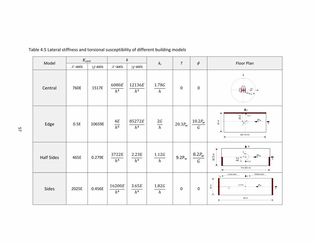
4.5 Lateral stiffness and torsional susceptibility of different building models ................ 57

4.6 Thermal analysis results of EPO .................................................................................. 62

4.7 Thermal analysis results of EDO ................................................................................. 67

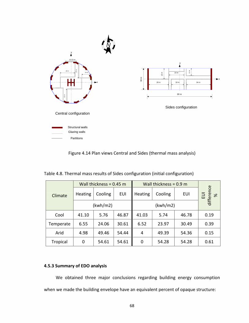
4.8. Thermal mass results of Sides configuration (initial configuration) .......................... 68

4.9 Thermal mass effect Sides configuration of 46% opaque .......................................... 69

5.1 lateral displacements result of BSS models ................................................................ 76

5.2 The lateral displacements result with SLLR ................................................................ 82

6.1 Embodied energy of the material used (for BSS & SLLR) ............................................ 85

6.2 The operational energy extreme differences in annual energy the cost ................... 90

6.3 Total material used cost index .................................................................................... 93

6.4 Summation all costs operational, embodied energies and material for fifty years life span ................................................................................................. 96

7.1 Energy demand verses SAR (N-S orientation)........................................................... 107

7.2 Energy demand ratio, EDR, (model of 1:4 aspect ratio) ........................................... 111

7.3 Sources of heat gain (Wh) in July- built to code envelope (model of 1:4 aspect ratio) .............................................................................................................. 113

xi

7.4 Breakdown heat gain (Wh) in July in Arid climate – regular glass envelope (model of 1:4 aspect ratio) ........................................................................... 114

xii

LIST OF FIGURES

Figure Page

3.1 Thermal mass material use in construction in Upper Egypt [24] ............................... 16

3.2 Heat gains through the thermal mass material: (a) Heat gain in winter; (b) Heat ispose in su er “after [25]” .............................................................. 17

. Heat transfer through a wall “after [2 ]” .................................................................. 20

.4 Heat gain/loss through an office buil ing co ponents “after [2 ]” .......................... 21

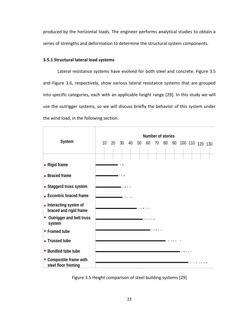
3.5 Height comparison of steel building systems [29] ...................................................... 23

3.6 Height comparison of concrete building systems [29] ............................................... 24

3.7 Outrigger-Braced Structures [30] ............................................................................... 25

3.8 a) outrigger system with a central core: (b) outrigger system with offset core[29] ........................................................................................................... 27

3.9 (b) cantilever bending of core; (c) tie-down action of cap truss [29] ......................... 28

3.10 One outrigger at top, z = L [29] ................................................................................. 30

3.11 Optimum locations of outriggers: (a) single outrigger; (b) two outriggers; (c) three outriggers; (d) four outriggers[29] ........................................................ 31

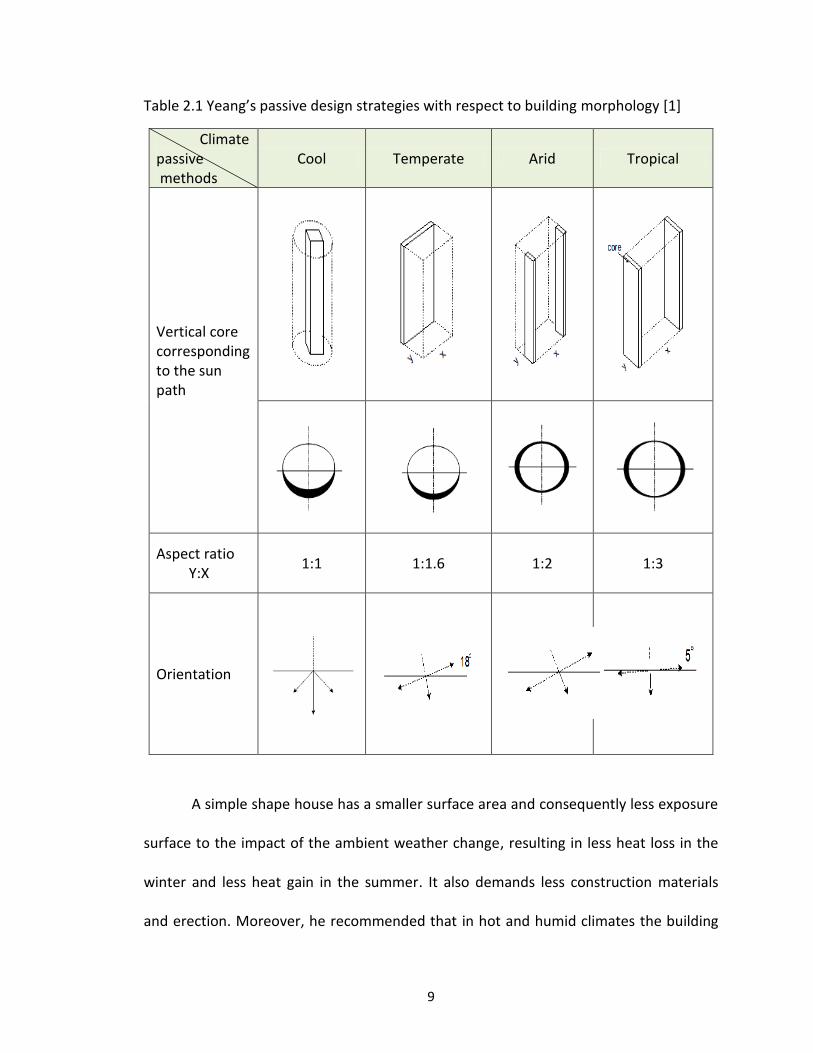
4.1 Proposal by K. Yeang for optimal floor-plan and placement of structural cores to minimize building energy consumption in four climates [1] ...................... 33

4.2 Plan views and an elevation of the buildings ............................................................. 35

4.3 Plan view of dodecagon shape- equivalent to the Central configuration .................. 42

4.4 Ecotect 3D models ...................................................................................................... 43

4.5 Sun-path diagram – buil ing’s walls sha ow.............................................................. 43

4.6 The thermal analysis result of the four models in the arid climate ........................... 46

4.7 The thermal analysis result of the four models in the cool climate ........................... 47

4.8 The thermal analysis result of the four models in the temperate climate................. 48

xiii

4.9 The thermal analysis result of the four models in the tropical climate ..................... 49

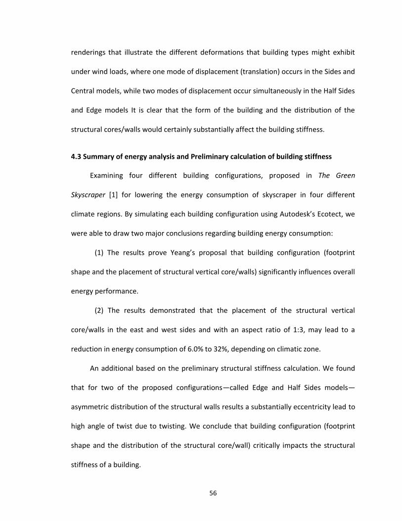
4.10 3D of how the different building types might deform under wind loads ................ 58

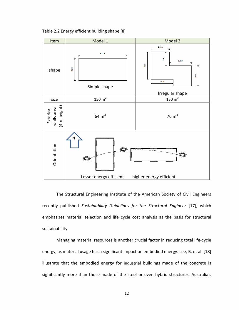
4.11 Plan views and an elevation of the buildings (EPO) ................................................. 61

4.12 The variance in EUI between the initial and EPO for the four configurations in each climate zone ....................................................................................... 63

4.13 Plan views and an elevation of the buildings (EDO) ................................................. 66

4.14 Plan views Central and Sides (thermal mass analysis) ............................................. 68

5.1 Torsional displacements: (a) Half sides; (b) Edge model ............................................ 76

5.2 Building plan views and schematic structural system for the buildings with three outriggers with/without belt trusses (connecting columns perpendicular to the plane of outriggers) ...................................................... 80

5.3 Lateral displacements at the roof (service wind loads Pw and 0.75 Pw) ................... 83

6.1 Financial comparison of the operational energy cost for a 50 year life span with respect to the Central configuration ...................................................... 91

6.2 Material cost index BSS and SLLR ............................................................................... 92

6.3 Financial comparison of the total cost for a 50 years life span with respect to the Central configuration ................................................................................ 97

7.1 Building orientation considered in this study ........................................................... 101

7.2 Building plan view and envelope thermal properties .............................................. 103

7.3 Sensitivity of EUI to the change in surface area ratio ............................................... 109

7.4 Monthly passive solar heat gain ratio (model of 1:4 aspect ratio) ........................... 112

1

CHAPTER 1

INTRODUCTION

For thousands of years, tall buildings and towers have fascinated human beings;

they have been built primarily for defensive or religious purposes as evidenced by the

Pharaonic temples (pyramids) of Giza, Egypt, the Mayan temples of Tikal, Guatemala,

the Kutub Minar of Delhi, India, and the gothic cathedrals of Europe.

In the modern era, high-rise buildings are a reality of contemporary life in cities

and there are several reasons for this. Urban real estate is a premium due to the lack of

available land, which drives up the cost of land and forces restrictions on indiscriminate

expansion (or sprawl) to preserve green space, natural habitats, or agricultural land.

High-rise buildings (vertical construction) present an effective way to reduce traffic

congestion in cities, as they can provide many services to citizens in a single building [1].

Rapid population growth of urban communities increases the need for housing, and

with limited buildable land, leads to pressure to develop high-rise residential

apartments. The limitations and the conditions of the terrain and topography in some

urban areas may make the construction of high-rise buildings the only viable solution.

This is particularly true for many cities in Asia and South America such as Rio de Janeiro

and Hong Kong [2]. As a result of the high concentration of businesses in city centers,

high-rise commercial buildings are a solution to keep these institutions as near to each

other as possible.

Meeting operational performance requirements and maintaining occupant

comfort in high-rise buildings is a challenging design problem. The energy demands for

2

large scale HVAC system (Heating, Ventilating, and Air Conditioning) loads are

significant. Not only are the site energy costs high, the attendant environmental

consequences of using non-renewable energy sources are great.

Improving the energy efficiency of high-rise buildings is a key component in

increasing the sustainability of the environment. More than one-thir of the worl ’s

energy consumption is attributed to the construction and building industry [3]. Given

the dramatically increased energy demand, there is a critical need to design and

construct buildings that are more sustainable. Energy efficient buildings minimize

building resource consumption, operations and life cycle costs, and can improve

occupant health and comfort [4].

High-rise buildings should be designed in a manner to reduce the need for fossil

fuels (oil, gas and coal) and promote greater reliance on passive/renewable energy

strategies. This concept is reflected in what is known these days as sustainable

architecture or green building. A green building is one that focuses on reducing the

impact of buildings on the environment. In general, a green building is one that meets

the needs of the present generation without compromising the ability of future

generations to meet their needs as well [1]. For designers and architects such as Reed

[5], green buildings are designed, implemented, and managed in a manner that places

the environment first. One of the key goals of the green building movement is to reduce

the material, constructional, and operational costs of buildings, and also reduce the

excessive depletion of natural resources. One way this is accomplished is by drawing on

the synergies between the building components (its materials and geometry) and the

3

local climate. Once building construction ends, a building becomes a part of its

environment, and is exposed to the effects of the sun, wind, and rain. If a building is

designed with these different environmental conditions in mind, it may take advantage

of available solar or wind energy or avoid its negative impact. This has the potential to

reduce energy loads, leading to reduced carbon dioxide emissions and ensuring a

healthy and sustainable building.

Substantial progress has been made towards improved energy efficiency through

design and technological innovations such as passive ventilation systems, daylighting

and sun shading, high performance heating, cooling, and ventilation (HVAC) systems,

and the introduction of novel materials to the building envelope. However, the impact

and influence of the structural system on building energy efficiency has been largely

neglected and therefore serves as the focus of this thesis. We consider whether

structural and energy performance considerations can be integrated and optimized

concurrently. And we analyze tradeoffs in the design of structural systems for both

structural and energy performance.

In his book The Green Skyscraper [1], architect Ken Yeang suggests that in

different climate zones, the structural core (structural wall) should be arranged in

different locations to reduce the yearly energy consumption of the building.

Furthermore, he argues the shape of the building footprint should be modified based on

the cli ate one in which the buil ing is to be constructe . In Yeang’s anal sis, three

parameters are varied - the shape of the building footprint, the placement of the

structural core or walls, and the orientation of the building. The first two (which we

4

define as building morphology) of these parameters have clear implications for

structural performance since buildings with asymmetric distribution of stiffness are

known to be susceptible to damaging torsional modes of vibration when subjected to

wind or earthquake loading. However, Yeang does not address the implications of

different footprints and core placements on structural performance. As for the third

parameter, building orientation has much less effect on the structural performance

unless the building is located where wind direction is strongly biased.

This study begins with an investigation of the relationship between structural

form and environmental performance, which use Yeang’s proposals as an approach to

limit the variables in this investigation. Four buildings are modeled in Ecotect Analysis

2011 correspon ing to four ajor cli ate ones. Each buil ing’s ther al properties are

assigned according to International Energy Conservation Code 2009 (IECC) [6]. These

four building configurations are examined under equivalent opaque surfaces in their

envelopes. The output for energy performance is presented in terms of annual heating

and cooling loads (Mwh/year). The results suggest that building morphology has a

significant effect on the annual energy consumption in a high-rise office building.

Second, the structural performance of the four study models is analyzed: 1) hand

calculations so preliminary estimating of the stiffnesses for the base structural system

(BSS) are made, and also based on the directional method [7]. We were able to make

preliminarily findings for what height BSS can meet the serviceability requirement

(according to the ASCE 7-10 for loading and lateral displacement limit); 2) structural

analysis and design by using SAP2000 (ASCE 7-10 is used to estimate wind loads). For a

5

set of given building conditions (loading and height, etc.), the results demonstrate that

supplementary lateral load resistance system (SLLR) is needed. An outrigger system is

used as the RLLS for the four buildings in this study. The output (under serviceability

control) is represented in terms of additional structural material needed for RLLS to

supplement the BSS in order to meet the specification.

Third, a cost analysis of these systems is conducted. The unit cost of a kilowatt-

hour based on the Energy Information Administration database (EIA), while the material

cost (material used in BSS and RLLS) have been estimated by using Reed Construction

data (RC means). The outputs (total operational and material cost for a building life span

of 50 years) show that buildings with asymmetric distribution of stiffness are the most

costly, in terms of both energy expenditures and additional material costs.

Fourth, the sensitivity of energy demand to two parameters of passive design

related to building layout and site are examined. The key parameters are building

footprint aspect ratio and building orientation, both of which are considered important

factors in passive design. Four high-rise office buildings (glazed curtain wall) with four

different aspect ratios (1:1, 1:2, 1:3, and 1:4) are thermally analyzed in four climate

zones: cool, temperate, arid, and tropical. Each buil ing’s ther al proprieties are

assigned according to 2009 IECC code. Energy demand is calculated for each model with

respect to two opposing orientations. The outcome shows that for buildings in Cool,

Arid, and Temperate climate zones, the energy demand may be considered marginally

sensitive to changes in aspect ratio, while in the Tropical climate zone, changes in aspect

ratio do not significantly affect energy demand. Moreover, the energy demand of high-

6

rise office buildings is not sensitive to the passive solar gain as long as the exterior

envelopes are built to IECC 2009 requirements for thermal performance.

In the following chapters, the details of these four studies are presented.

Chapter 2 provides a literature review of existing scholarship in this area as well as a

thorough explanation of Yeang’s proposal. Chapter 3 presents background about

thermal properties, referring to the green building, and mentioning about the lateral

resistance systems for tall buildings. Chapter 4 focuses on the energy analysis and the

preliminary structural calculations. Chapter 5 frames the structural modeling, analysis

and design using SAP2000. Chapter 6 focuses on the cost calculation (operational,

embodied energy and material costs). Chapter 7 addresses the sensitivity of energy

demand to two parameters of passive design related to building layout and site. Finally,

chapter 8 illustrates our conclusions, recommendations, and future work.

7

CHAPTER 2

LITERATURE REVIEW

The design of high performance buildings is becoming increasingly urgent, and

efforts are being made by engineers and architects to reduce the environmental impact

of buildings to conserve resources and secure our energy future. In the present study,

we consider the building morphology and its influence on energy and structural

performance. However, there is a lack of research to support a correlation between

energy performance and structural performance.

In his book The Green Skyscraper [1], architect Ken Yeang suggests that building

morphology, i.e. aspect ratio, the shape of the building footprint, orientation, and

placement of structural vertical core/walls can be designed to maximize passive-mode

systems. For Yeang, there is an ideal aspect ratio for each different climate zone, which

is presented in Table 2.1. He states that for the four major climate zones, the long axis

of the footprint should be oriented east-west except in a cool climate. The rationale is to

control the amount of exposed area to the sunlight for each individual side of the

building.

Building orientation is another critical aspect of passive design. The goal is to

orient the building in accordance to sun path and wind direction. Orientation helps to

increase or decrease the heat gained from the sun by either maximizing or minimizing

the amount of time that the building is exposed to direct sunlight. Yeang provides an

example for a building located in the tropical climate zone: to reduce insolation (i.e.

direct solar heat gain), the short axis of the building footprint should be on the north-

8

south axis and the building oriented with 5o north of east. Also, he suggests that for

each one of the major climate zones there is a critical angle of orientation for passive

design, see Tablet 2.1.

The third aspect of passi e esign in Yeang’s book is the placement of structural

vertical cores. Choosing the ideal position of the structural vertical cores with regard to

the climate zones may help to modulate building interior temperatures. In principle,

heavy and opaque structural cores provide shade and thermal mass to the building,

potentially helping to keep it cool or to restrict heat penetration in the building. Thus,

one would place the vertical cores to avoid or accommodate direct solar gain according

to a climate zone. Yeang suggests that in a cool climate where solar gain can help to

offset heating energy costs, it is optimal that the structural core is placed in the center

of the building where it cannot block an of the sun’s irect ra s. In a temperate zone

the structural core is placed on the north face, in a tropical zone cores are placed on

both east and west sides and in an arid zone cores cover 50% of east and west sides, see

Table 2.1.

To reduce energy consumption using passive methods in high-rise structures,

Yeang provides a set of directives: for each one of the major climate zones, the

structural walls should be arranged in different locations and the shape and the

orientation of the building should be modulated to reflect the unique demands of the

climate [1]. Walker [8] shows that simple shaped houses are typically more efficient to

cool and heat than houses with irregular shapes (Table 2.2).

9

Table ‎2.1 Yeang’s passi e esign strategies with respect to buil ing morphology [1]

Climate passive methods

Cool Temperate Arid Tropical

Vertical core corresponding to the sun path

Aspect ratio Y:X

1:1 1:1.6 1:2 1:3

Orientation

A simple shape house has a smaller surface area and consequently less exposure

surface to the impact of the ambient weather change, resulting in less heat loss in the

winter and less heat gain in the summer. It also demands less construction materials

and erection. Moreover, he recommended that in hot and humid climates the building

10

shape should be designed to minimize solar heat gain to reduce cooling demand.

Furthermore, multi-story homes are generally more efficient because they have less

exposure area to the sunlight compared to same size single-story houses. Moreover,

building elongated in an east-west direction could greatly affect the overall energy

efficiency (Table 2.2).

Cheung et al. [9] published a study in 2004 that describes an investigation of the

effects of six passive design strategies (insulation, thermal mass, glazing type, window

size, color of external wall and external shading devices) on the annual cooling energy

for a high-rise apartment building in Hong Kong. This study shows that a reduction in

energy consumption for cooling load of 31.4% can be obtained, as a result of modifying

building envelope to match the local climate. However, this achievement is specific to

this building type and this particular climate.

Jones et al. [10] widely studied passive solar design and the balancing between

the energy conservation and the solar energy strategies to save in the cost of annual

energy demand with respect to the climates. Furthermore, he developed a method for

the optimum mix of energy conservation and solar energy. He emphasized that the

esigner ecision shoul alwa s in ol e the “tra e-off between the cost of the

i pro e ent ersus the increase perfor ance.”[10] He recommended that energy

conservation is more appropriate and less solar where cooling is significantly demanded.

Also, he recommended that the features of passive solar heating can increase cooling

loads in summer time, therefore shading tactics to reduce this effect should be

considered. Mazria [11] provided a complete guide to passive solar home, greenhouse

11

and building design, which illustrates many different applications of direct heat gain

concepts for both commercial and residential buildings. In terms of building shape he

recommended that for all climates the sufficient building elongated is in an east-west

direction, which results in more exposed surface area facing south, minimizing heating

needed in winter and cooling in summer. Also he emphasized that in the case of

climates where heating is needed in winter, place the building on the site that receives

the most sun during the hours of maximum solar radiation 9:0 am to 3:0 pm “to insure

that-the, outdoor areas and gardens placed to the south will have adequate winter sun,

and help minimize the possibility of shading the building in the future by off-site

developments” [11].

A number of studies have focused on natural ventilation design strategies to

reduce energy loads. Chow [12] shows that a structural wall projecting from the building

façade could guide prevailing winds to drive passive ventilation of a tall building. Li and

Mak [13] used simulation to evaluate the performance of wind catcher devices designed

for passive ventilation. Mak, C.M., et al. [14] investigated the effect of wing walls on

passive ventilation and found potential synergies between the structure and

environmental performance.

Finally, the structural engineering profession has been attempting to define the

proper role for the structural engineer in the pursuit of sustainability of the built

environment. Anderson & Silman [15] and Webster [16] identify how the structural

engineer may work with an integrated design team of architects, engineers, builders and

owners to make the structure sustainable.

12

Table ‎2.2 Energy efficient building shape [8]

Item Model 1 Model 2

shape

Simple shape

Irregular shape

size 150 m2 150 m2

Exte

rio

r w

alls

are

a (4

m h

eigh

t)

64 m2 76 m2

Ori

enta

tio

n

Lesser energy efficient higher energy efficient

The Structural Engineering Institute of the American Society of Civil Engineers

recently published Sustainability Guidelines for the Structural Engineer [17], which

emphasizes material selection and life cycle cost analysis as the basis for structural

sustainability.

Managing material resources is another crucial factor in reducing total life-cycle

energy, as material usage has a significant impact on embodied energy. Lee, B. et al. [18]

illustrate that the embodied energy for industrial buildings made of the concrete is

significantly more than those made of the steel or even hybrid structures. Australia's

N

13

guide to environmentally sustainable homes [19] and TecEco sustainable technologies

[20], show that the concrete in its basic form has relatively low embodied energy, but its

high usage in construction results in higher total embodied energy than any other

material. According to the American Institute of Architects Sustainable Design Resource

Guide, 90% of 1.0 MJ/kg embodied energy of concrete of compressive strength 17.5

MPa is attributable to the production of Portland cement. Ashley, E. and Lemay, L. [21]

show that the embodied energy of virgin imported structural steel is 35.0 MJ/kg, while

recycled steel has an embodied energy of 10.1 MJ/kg. In his study Ken Yeang [1]

illustrates that the amount of embodied energy of concrete-frame structure is almost

the same as that from the steel structure, but the concrete structure is less recyclable at

the end of its useful life than the steel structure.

However, these publications promise to significantly affect the way structural

engineering is practiced, yet none the above studies directly address the interplay of

structural form and energy efficiency, which is our primary interest.

14

CHAPTER 3

BACKGROUND

3.1 Thermal mass

Thermal mass may be defined as the buil ing’s aterials ability to store heat, i.e.

its thermal storage capacity, for extended periods. A material with good thermal mass

will absorb heat from an available source like sunlight during the daytime or from the

heating system in the building, store it, and release it when the sun sets and air

temperature drops or the other source turns off. The ain characteristic of a aterial’s

thermal mass is its density and specific heat; the capacity to retain heat varies for

different materials. The material that has higher density and specific heat capacity has a

higher thermal mass, which can be calculated as following [22].

Where M is the mass of substance, T change in temperature, and Cp is the specific

heat of substance.

3.2 Thermal mass properties

Materials with high density typically have a higher thermal mass; for example

normal weight concrete has higher thermal mass than light weight concrete, mod brick

has low thermal mass, and insulation materials have almost no thermal mass. A good

thermal mass material with high density characteristics also has to be conductive.

However, if conductivity is too high (e.g. steel) energy is absorbed and given off too

quickly, compromising its ability to be a heat sink for thermal storage.

15

3.3 Thermal mass in Buildings

There are some known thermal mass materials built-up in building elements

such as water, soil, rock, concrete, brick, cement, and ceramic tile. These represent the

bulk of building construction materials. In buildings with mechanical heating,

ventilation, and air conditioning (HVAC) systems, the presence of a thermal mass

material may affect the heating and cooling loads because it can lead to raised or

lowered temperatures inside the building. Thermal mass within the insulated building

envelope may also help to reduce fluctuations and dampen extremes in temperature

inside the building [23].

In ancient times people built their shelters against earth berms and hillsides to

take advantage of the earth as a thermal mass to protect them from the heat during the

day and cold at night. During the day, building surfaces (walls and roof) that are exposed

to direct sunlight must have the capacity to absorb solar energy and by the night they

radiate this energy out as heat. The thermal mass absorbs thermal energy passively

during the day and releases this stored energy at night. In these kinds of buildings,

maintaining thermal comfort for occupants inside buildings depends largely upon the

thermal mass of the walls and roofs. In climates with low heating energy demands such

as the temperate-arid zone of Upper Egypt [24], using materials with high thermal

storage capacity in their construction helps to modulate interior temperatures (see

Figure 3.1).

Today, thermal mass is usually used in conjunction with passive design

techniques [25]. Indeed, thermal mass may help to mitigate operational energy loads

16

and is most appropriate where there is a big difference between day and night outdoor

temperatures. However, in the winter time thermal mass sometimes might not be

efficient, becomes buildings often use mechanical heating systems, and the thermal

mass might absorb some heat produced from heating system [23].

Figure 3.1 Thermal mass material use in construction in Upper Egypt [24]

Figure 3.2 shows how the heat is gained by allowing sunlight and is stored in the

thermal mass during the day and released in the night time which leads to warming the

room. This is a desired solution if nighttime heating is desired. On the other hand, in the

summer, if nighttime heating is not desirable, then strategies to cool the thermal mass

have to be implemented. One solution is to allow for air cooling, that is, convective

Use thermal mass material keeps rooms cooler

Use thermal mass material Keeps water cooler

17

currents to pass over the thermal mass to draw out the stored energy resulting

comfortable atmosphere inside the building[25].

Figure 3.2 Heat gains through the thermal mass material: (a) Heat gain in winter; (b) Heat dispose in summer “after [25]”

Thermal mass in a building envelope slows down heat flow through the walls,

roof, and floor, potentially allowing a reduction in insulation requirements. Buildings

constructed with materials that have high thermal mass like concrete could have a

unique energy saving advantage because of their inherent thermal mass. These

materials absorb energy slowly and hold it for much longer periods of time, and then

release it as heat energy.

Heat gainHeat

releasedRad

ian

heat

Winter

Sun

Breezes

Heat

released

Summer

Sun

(a)

(b)

18

3.4 Thermal transmission through building

Most of the common building materials that are used in contemporary

construction absorb and transfer heat. The total amount of heat transferred through the

building elements can be determined by calculating the resistance to heat transfer (R-

value) of each material in the building assembly [26].

3.4.1 Heat transfer

Heat transfer is flow of heat energy from a high temperature body to a lower

temperature body, which is fundamental to the second law of thermodynamics. There

are three primary mechanisms of heat transfer: conduction, convection, and radiation

(see Figure 3.3). Conduction is defined as the transfer of heat energy from the higher

temperature to lower temperature particles that are in contact. This mode of heat

transfer occurs in a stationary material (solid bodies and non-movable fluids),

conductive heat transfer is given by:

Where is the rate of heat flux by conduction (Watts), k is the thermal conductivity

(W/m k), A is the surface area (m2), ∂T/∂x change of te perature with respect to x

which is wall thickness (k/m). Heat transfer by convection is a combination of

conduction and fluid motion, where convection occurs wherever a surface is in contact

with a fluid at a temperature that is different from its own. Convective heat transfer is

given by:

19

Where is the rate of heat flux by convection (Watts), h is the heat transfer coefficient

(W/m2 k), ΔT is the ifference in the surface te perature (T surface and T ambient) (k). Heat

transfer by radiation occurs by electromagnetic waves that are emitted from a hot body

towards cold body (such as heat transferred from the sun to the earth). Radiation heat

transfer is given by:

Where is the heat flux by radiation, is the Stefan- Boltzmann constant (W/m2 k4).

Transmission of heat through a wall can be summarized as: Heat transfer by convection

Qc and radiation QR from the hot air (air film) surrounding the external wall surface.

Then heat transfer by conduction Qk through the wall. Once the heat reaches the

internal surface, it is transferring again by convection QRi and radiation Qci from the wall

surface to the cold air and surrounding surfaces inside the room. Where the rate of heat

transfer mainly depends on the wall thermal resistance property, which is R-value (R=

1/U) the resistance to heat flow, is equal to the inverse of thermal conductance (U-

value) which may be defined as the amount of heat flow of through a material. Note,

high R-Value materials could be used as insulation materials.

3.4.2 Office building heat gain

Heat gain is the thermal energy that a room may gain from external and internal

sources. External sources of heat gain are heat transferred to indoors due to the

difference between outside and inside temperature. This gain occurs through the

building envelope walls, ceiling, windows, ventilation systems, and air leakage. Internal

20

sources of heat gain are the heat generated by occupants, the heat produced by

lighting, and the heat resulting from the equipment (Figure3.4) [26].

Figure 3.3 Heat transfer through a wall “after [27]”

Daytime heat flow through an exterior wall is due to solar radiation on exterior

surface and the outside ambient temperature. Nighttime heat gain through a wall is

typically a result of thermal lag effects, as a result of thermal mass heat storage. A wall

of high thermal capacity may considerably dampen the inside temperature swings,

when ambient temperature fluctuates , whereas, a wall of low thermal capacity has

little damping effect; thus any variations in outside temperature will almost immediately

affect the inside temperature.

Qk

QR

Qc

Hot air

Tambient

Cool air

Tindoor

Wall

R-value

QRi

Qci

x

21

Heat gain through glass windows may occur in two ways [26] a) Sensible

transmission through glass (caused by the difference between inside and outside

temperatures), b) Solar gain through the glass. This gain depends on building orientation

as sun-path and location of windows on a building greatly influence the extent of direct

solar heat gain through glazed surfaces. Solar heat gain can mainly be controlled by the

solar heat gain coefficient of the glass (SHGC) [6].

Figure 3.4 Heat gain/loss through an office building components “after [27]”

Heat transfer through unintended air exchange is a result of infiltration or

exfiltration. Infiltration occurs through the small cracks and improper seals on windows

and doors. The allowable infiltration rate is 0.5 air change per hour for most air-

Conduction through opaque surfaces

Conduction through glass

cooling

Heating

Equipment

gains

Lighting gains

Occupacy

gains

Solar gain

Ventilation heat loss and gain

Daylighting

22

conditioning cases [28] and may be less (0.25 air change per hour) in case of high

performance buildings or if special measures have been taken to prevent infiltration.

The heat gain as a result of occupants in a building is a combination of sensible

and latent heat. Sensible heat gains from occupants results from the difference between

the human body temperature and the temperature of the air inside the room. Latent

heat is characterized by an increase in the moisture content of the air, which can be

attributed to occupant respiration. Heat gain by the occupants depends on the number

of people in the room and the rate of heat released by each person, which depends on

the degree of activity. Heat gain from lighting depends on light equipment efficiency and

lighting level. Heat gain from equipment depends on number of machines and their

efficiency [26, 28].

3.5 Design and analysis of tall building

During the design and construction process, structural engineers and

architectural designers work together on the building design and on the elements of

construction such as the location of partitions, stairs and elevators, positioning of

columns and lateral resistance systems, as well as choice of materials. The structural

engineer calculates the gravity loads and identifies the forces which will be generated

on the building due to wind and earthquake loads.

The challenge for structural engineers is to design a lateral resistance system

that fulfills the requirements of architectural design. This task starts with estimating the

lateral loads and identifying the full extent of possible deformations that can be

23

produced by the horizontal loads. The engineer performs analytical studies to obtain a

series of strengths and deformation to determine the structural system components.

3.5.1 Structural lateral load systems

Lateral resistance systems have evolved for both steel and concrete. Figure 3.5

and Figure 3.6, respectively, show various lateral resistance systems that are grouped

into specific categories, each with an applicable height range [29]. In this study we will

use the outrigger systems, so we will discuss briefly the behavior of this system under

the wind load, in the following section.

Figure 3.5 Height comparison of steel building systems [29]

10 3020 90807040 50 60 130110100 120

Number of stories

System

Rigid frame

Braced frame

Staggerd truss system

Eccentric braced frame

Interacting systen of

braced and rigid frame

Outrigger and belt truss

system

Framed tube

Trussed tube

Bundled tube tube

Compostite frame with

steel floor freming

24

Figure 3.6 Height comparison of concrete building systems [29]

3.5.2 Outrigger-Braced Structures

The main information summarized from the book written by Bungale S. Trananath

[29] (Wind and Earthquake Resistant Buildings: Structural Analysis and design). The

outrigger system is a central core made of braced frames or shear walls, with trussing or

gardening hori ontal cantile er “outrigger” connecting the core to the outer colu ns.

Joining the columns to the core by those outriggers makes the structure behave as

partly composite cantilever. The outrigger systems may be formed in any combination

10 3020 90807040 50 60 110100 120

Number of stories

System

Flat slab and columns

Flat slab and shear walls

Flate slab, shear walls and

columns

Rigid frame

Widely spaced perimeter

tube

Gigid fram with haunch

griders

Core supported structres

Shear wall -frame

Closely spaced perimeter

tube

Coupled shear wlls and

beams

Exterior diagonal tube

Perimeter tube and interior

core walls

Modular tubes

Shear wall -Haundh girder

frame

25

of steel, concrete, or composite construction [30, 29]. Under lateral loading, the

outriggers restrain the core against overturning through tension in the windward

columns and compression in the leeward columns (Figure 3.7). Outrigger-braced

structures have been used in building up to 70 stories [29].

Figure 3.7 Outrigger-Braced Structures [30]

3.5.2.1 Outrigger systems behavior

As we mentioned the core is connected to the edge columns by relatively stiff

horizontal members (the outrigger). These outriggers may be located with extending on

both sides; it could also be located on one side of the building with outriggers extending

to the building columns on one side (Figure. 3.8) [29, 30]. When subjected to lateral

loads, the basic structural response is: the column-restrained outriggers resist the

26

rotation of the core, resulting in smaller lateral deflections and moments in the core.

The external moment is now resisted by the axial tension and compression of the

exterior columns connected to the outriggers, not only by the bending of the core. As a

result, the effective depth of the structure is increased when it flexes as a vertical

cantilever, “by the development of tension in the windward columns, and by

compression in the leeward columns” [29].

To assist in restraining the outriggers one usually uses other peripheral columns,

which can be done by attaching a eep span rel gir er, or a truss “belt truss,” [29],

around the structure at the levels of the outriggers. One or two stories usually comprise

the depth of the outriggers and belt truss [30].

To simplify the outrigger system behavior, consider a building stiffened by a

story high outrigger at the top, as shown in Figure 3.9. The restraining action produced

by the cap truss generates a restoring couple at the building top, resulting in a point of

contra flexure in its deflection curve. Thus, the bending moment in the core is reduced

by this reversal in curvature. The tension and compression forces work as a couple to

produce rotation opposite to the rotation produced by the core. Therefore, the

outrigger at the top may be considered a restraining spring located at the free end [16].

With the assumption that the cap truss is rigid, “the axial elongation and

shortening of columns is equal to the rotation of the core multiplied by their respective

distances fro the center of the core” [29]. Considering the distance of the equivalent

column is d/2 from the center of the core, the axial deformation of the columns would

be then equal to (ϴ X d/2), where ϴ is the core rotation.

27

Figure 3.8 a) outrigger system with a central core: (b) outrigger system with offset core[29]

With the equivalent spring stiffness being calculated for unit rotation of the core, the

axial deformation of the equivalent columns is equal to d/2 units. The corresponding

axial load P in the columns is as following:

where A is the area of columns; E is the modulus of elasticity; d is the distance between

the exterior columns; L is the building height (Figure. 3.10). The rotational stiffness of

the outrigger at the top is given by the axial load in the equivalent columns multiplied by

their distance from the center of the core.

28

Figure 3.9 (b) cantilever bending of core; (c) tie-down action of cap truss [29]

The rotational stiffness (K) for the two equivalent columns is located at a distance d/2

from the core.

To calculate the lateral deflection, the rotation compatibility condition at z = L can be

written as:

where is the rotation of the cantilever at z = L due to a uniform lateral load W, in

radians; is the rotation due to spring stiffness is in a direction opposite to the rotation

due to external load, located at z = L, in radians; is the final rotation of the cantilever

at z = L, in radians. For a cantilever with uniform moment of inertia I and modulus of

elasticity E subjected to uniform load W.

29

If M1 and K1 represent the moment and stiffness of the spring located at z =L, then Eq.

(3.3) can be rewritten as

(

)

( )

The resulting deflection at the building top can be obtained by superimposing the

deflection of the cantilever due to external uniform load W, and the deflection due to

the moment induced by the spring, thus:

(

)

With the same concept and based on the expression for lateral deflection y, at distance

x measured from the top and is equal to (L - z); where for a cantilever subjected to a

uniform lateral load ((Figure. 3.10) is given by:

30

Figure 3.10 One outrigger at top, z = L [29]

Thus, if M2, M3, and M4 are the moments of the spring corresponding to different

heights, we can calculate the lateral deflation at any height, so, lateral deflation at z

=3L/4, z =L/2, and z =L/4 are:

(

)

(

)

(

)

3.5.2.2 Optimum Locations of Outrigger Trusses

It’s been reco en e that the optimum level of the outriggers for minimizing

the drift for a single outrigger is at approximately mid-height (Figure. 3.11). A two-

outrigger system would have one placed at 1/3 and the other placed at 2/3 of the

building height [30]. For a three-outrigger system, they should be at the 1/4, 1/2, and

3/4 heights, and so on. Therefore, for the optimum performance of an n-outrigger

31

structure, the outriggers should be placed at 1/n + 1, 2/n + 1, 3/n + 1, 4/n + 1… n/n + 1

height locations [29].

Figure 3.11 Optimum locations of outriggers: (a) single outrigger; (b) two outriggers; (c) three outriggers; (d) four outriggers[29]

32

CHAPTER 4

INVESTIGATING THE EFFECT OF BUILDING MORPHOLOGY AND CORE PLACEMENT ON ENERGY PERFORMANCE OF SKYSCRAPER OFFICE BUILDINGS

4.1 An approach

In his book The Green Skyscraper [1], architect Kenneth Yeang suggests that in

different climate zones the structural core should be arranged in different locations to

reduce the yearly energy consumption of the building. He also argues the shape of the

building footprint should be modified based on the climate zone in which the building is

to be constructed (Figure 4.1). In Yeang’s anal sis, three are para eters arie - the

shape of the building floor plan, the placement of the structural cores/walls, and the

orientation of the building. The first two of these parameters have clear implications for

the structural performance, while building orientation has much less effect on the

structural performance unless the building is located where wind direction is strongly

biased.

In the present work, we consider two parameters, the shape of the building

footprint and the placement of the structural cores (structural walls, to evaluate the

structural and energy performance of four different building morphologies in four

different climate zones. We then present the results of structural and energy

consumption calculations for each of the sixteen morphology/climate scenarios.

In this study, as in Yeang’s, two ain characteristics are o ulate to opti i e

energy performance: the position of the vertical structural core/walls and the aspect

ratio and shape of the building footprint.

33

4.1.1 Description of building models variables

All other morphological descriptors such as the square footage, number of

stories, building height, occupancy, schedules, and envelope materials, for the four

skyscraper office buildings are constant. All buildings modeled in this study are 200 m in

height, 50 stories that are 4.0 m floor to floor height, with a total conditioned floor area

of 135000 m2. Figure 4.2 shows the plan views for these models, and the locations of

the primary mass (opaque surfaces) and the glazing walls (transparent surfaces) for each

configuration. The primary material for the structural core/wall (opaque walls) is

reinforced normal weight concrete, and the glazed (curtain) walls are two layers of

standard glass with 10 % metal framing.

Figure 4.1 Proposal by K. Yeang for optimal floor-plan and placement of structural cores

to minimize building energy consumption in four climates [1]

x

y

x

y

Climate Cool Temperate Arid Tropical

1:1.6 1:2 1:31:1Aspect ratio

Y:X

x

yN

y

x

y x yx

y

x

core wall

34

To simplify the analysis, we have neglected the effect of surrounding buildings

and of building orientation, in essence assuming that the buildings are erected on flat

open ground and are aligned with the cardinal directions.

The materials selected for the exterior envelope of all four models meet the

requirements of thermal resistance of the 2009 International Energy Conservation Code,

IECC [6], for each specific climate zone. There are three different material palettes (with

associated thermal resistances) for the four buildings. In other words, there is a

prescribed material palette for the buildings in the tropical zone 1, for buildings in the

temperate zone and arid zones (both zone 3), and for buildings in cool zone 5. Structural

layers and thermal resistance of the material are presented in Table 4.1.

All four building morphologies are simulated in each of the four major climate

zones (cool, temperate, arid, and tropical, according to the Koppen classification [31]).

Additionally, we have selected specific cities as representative of the conditions in each

climate zone, and use the climatic conditions at these four cities in the energy

performance simulations: Boston, Massachusetts for the cool zone, Sacramento,

California for the temperate zone, Las Vegas, Nevada for the arid zone, and Honolulu,

Hawaii for the tropical zone. The climate characteristics for the representative cities are

provided in Table 4.2 [32].

Building energy consumption is highly dependent on occupancy and scheduled

usage of the interior space. Since our goal is to isolate the influence of building

morphology on energy consumption, we assume that occupancy and scheduling

characteristics are constant across all climate zones and building types.

35

Plan view -Central configuration[ 100% glazed curtain walls]

65.75 m

41

m

y

x

Plan view -Edge configuration[31% opaque ; 69% glazed curtain walls]

21 m

20 m

20.5

m

18 m

17

m

19 m

Core/walls: opaque surfaces

Non-core: glazed curtain walls

Partitions

Note: - Percentages given are only for the

building envelope.

0.0 18 m 36 m 54 m 72 m

73.50 m

36

.75

m

x

y

Plan view -Half Sides configuration

[17% opaque ; 83% glazed curtain walls]

23 m28 m

18.4

m 20 m 12

.5 m

15.6 m

90 m

30

m x

y

Plan view -Sides configuration

[25% opaque ; 75% glazed curtain walls]

34 m28 m

15 m 23 m 1

.5 m

18 m

r=29.30 m

x

y

14 m20 m

21

m

20

m

x

Elevation

50

@ 4

m

15

m

15 m

Figure 4.2 Plan views and an elevation of the buildings

36

Table 4.1 Structural layers and thermal resistance of the materials

Ele

men

t Material

Layers

Zone 1 (Tropical)

Zone 3 (Arid &Temperate)

Zone 5 ( Cool)

U-v

alu

e

W/m

² K

R-v

alu

e

m²

K/W

U-v

alu

e

W/m

² K

R-v

alu

e

m²

K/W

U-v

alu

e

W/m

² K

R-v

alu

e

m²

K/W

Zone 1 (Tropical)

Zone 3 (Arid &Temperate)

Zone 5 ( Cool)

Co

res

wal

ls

*450 mm concrete III

450mm concrete III 22 mm polystyrene foam 10 mm plaster in either side

450 mm concrete III 45 mm polystyrene foam 10 mm plaster in either side

1.65 0.61 0.74 1.36 0.49 2.05

Gla

zin

g w

alls

*6 mm single glazed metal framing

6 mm double glazed metal framing, 15 mm gap with low-conductance gas fill

6 mm double glazed metal framing, 13 mm gap with low-conductance gas fill

6.81 0.15 3.40 0.294 9.3 0.107

Ro

of

27 mm Aggregate 6 mm asphalt 100 mm concrete III 19 mm poly. foam 10 mm plaster

27 mm Aggregate 6 mm asphalt 100 mm concrete III 27 mm poly. foam 10 mm plaster

27 mm Aggregate 6 mm asphalt 100 mm concrete III 27 mm poly. foam 10 mm plaster

0.37 2.71 0.267 3.75 0.267 3.75

(Continue)

37

Ele

men

t Material

Layers

Zone 1 (Tropical)

Zone 3 (Arid &Temperate)

Zone 5 ( Cool)

U-v

alu

e

W/m

² K

R-v

alu

e

m²

K/W

U-v

alu

e

W/m

² K

R-v

alu

e

m²

K/W

U-v

alu

e

W/m

² K

R-v

alu

e

m²

K/W

Zone 1 (Tropical)

Zone 3 (Arid &Temperate)

Zone 5 ( Cool)

Flo

or

susp

end

ed c

on

cret

e

10 mm ceramic tiles 5 mm screed 100 mm suspended concrete floor 50 mm air gap 10 mm plaster ceiling underneath

10 mm ceramic tiles 5 mm screed 100 mm suspended concrete floor 20 mm polystyrene 50 mm air gap. 10 mm plaster ceiling underneath

10 mm ceramic tiles 5 mm screed 100 mm suspended concrete floor 40 mm polystyrene 50 mm air gap. 10 mm plaster ceiling underneath

1.81 0.55 0.86 1.17 0.27 3.75

Slab

on

gr

ou

nd

100mm concrete 5 mm screed 10 mm ceramic tiles

100mm concrete 5 mm screed 10 mm ceramic tiles

100mm concrete 5 mm screed 10 mm ceramic tiles

0.88 1.14 0.88 1.14 0.88 1.14

Par

titi

on

80mm framed wall as air gap 10mm plaster board either side

80mm framed wall as air gap 10mm plaster board either side

80mm framed wall as air gap 10mm plaster board either side

2.21 0.45 2.21 0.45 0.21 0.45

* The element would consist of some layers only that shown in the layers column

38

Specifically, we treat the thermostat range, internal design conditions, occupancy,

infiltration rate, and hours of operation as fixed control variables (Table 4.3).

4.1.2 The thermal analysis

For the remainder of this dissertation, the proposed configurations are named

depending on where the structural cores/walls are placed (opaque walls): Central for

cool zone; Edge for temperate zone; Half Sides for the arid zone; Sides for the tropical

zone.

4.1.3 The modeling

Auto esk’s Ecotect energ si ulation package was use for the thermal analysis.

Ecotect 2011 is a comprehensive concept-to-detail sustainable building design. It is a

popular program used by architects, its modeling procedure is simple, it is easy to

rapidly manipulate the properties of models, and it consumes a reasonable amount of

analysis time for large models. The Ecotect procedure starts with creating a three

dimensional shell that represents the building form. This can be done in one of two

ways: (1) draw plans representing the boundary of the rooms, continuing room by room

to form a 3D model; or (2) import the model as gbXML file from a different 3D modeling

program such as Revit. For this anal sis, we prepare the buil ing’s geo etr in Re it

2010, and then imported the 3D model as surfaces and rooms to Ecotect 2011. After the

i port, ther al properties are assigne to the buil ing’s en elope an the anal sis

proceeds. The basic material of an element (concrete wall, slab, glazing wall, etc.) is

39

assigned then the resistance (R-value) of the insulation is applied, according to

specifications of IECC code as presented in Table 1.

Table 4.2 Description of the climate zones characteristics for the representative cities

City

Characteristics

Boston [Cool]

Sacramento [Temperate]

Las Vegas [Arid]

Honolulu [Tropical]

Ave

rage

te

mp

erat

ure

s

hig

h

23.3 °C 24 - 32 °C 34 - 40 °C 27-32 °C

low

-1.5 °C 7.7- 16 °C 21–26 °C 19-24 °C

Dry

bu

lb

tem

per

atu

re

max

imu

m

37.2°C [on Jul 9]

42.0°C [on Jun 14]

44.4°C [on Jul 4]

33.3°C [on Sep 2]

min

imu

m

-20.0°C [on Jan 23]

-2.0°C [on Feb 2]

-3.3°C [on Feb 16]

13.3°C [on Feb 12]

An

nu

al d

egre

e-d

ays

[18

°C b

asel

ine]

coo

ling

490 670 1904 2524

hea

tin

g

3120 1436 1234 0.0

Average daytime 11 hr, 45 min 12 hr, 24 min 11 hr, 15 min 12 hr

Average nighttime

12 hr, 15 min 11 hr, 36 min 12 hr, 45 min 12 hr

Average annual rainfall

1,080 mm plus

1,060 mm of snowfall

545 mm 110 mm 460 mm

Maximum wind speed

21.6 m/s [on Sep 6]

17.0 m/s [on Mar 4]

20.6 m/s [on Apr 12]

13.4 m/s [on Nov 15]

40

Table 4.3 Thermal analysis conditions

Parameters Values Description

Active system Full Air conditioning

Active system for providing

heating and/or cooling

Thermostat range 18 – 26 oC comfortable range

Occupancy People 12 m2/p

office - typical square area

for one person

Activity 70 W/p sedentary

Internal design conditions

clothing 1 clo/p light business suit

Humidity 60% comfortable Humidity

Air speed 0.5 m/s pleasant breeze

lighting level 300 lux luminous flux per unit area

Infiltration rate

Air change rate 0.5 /hr office - typical value

Internal heat gain 10 W/ m2 lighting and equipment

Hours of operation Schedule 8 am-18 pm ( week)

The next step is to assign a weather file which corresponds to the climatic zones

selected for this study and to provide occupancy and scheduled usage data. And finally,

the program can calculate monthly and annual heating and cooling loads according to

given climate conditions, (Figure 4.4).

4.1.4 Modeling assumptions

For the purpose of the present analysis, several assumptions are made: a) all the

buildings have equivalent square footage, height, material usage, and thermal

properties; b) all the buildings are oriented 90o with the north; c) to simplify the

41

analysis, the circular shape of Central configuration has been replaced by dodecagon

(12-sided) shape with equivalent floor area as shown in Figure 4.3.

Ecotect calculate the heating and cooling loads based on the admittance

procedure, which assume that the fluctuations between the external and internal loads

can be presented by the sum of the steady-state component. This method is insensitive

to the rapid change in neither temperature nor long-term heat storage. However, this

method has no restrictions on the number of thermal zones or building geometry [26].

The analysis based on the local (outside and inside) mean and the fluctuations in

the temperature around this mean, when outside temperature or solar load change the

internal air temperature fluctuate in a similar way. “The steady-state component is

calculated using a three-node model incorporating an environmental temperature node

to which all zone surfaces are connected by a combined radiant and convective

conductance” [ ].

4.1.5 The analysis

The thermal analysis involves examining each of the four models (Central, Edge,

Half Sides, and Sides) in each of the four climatic zones (cool, temperate, arid, and

tropical). This constitutes sixteen different simulation runs, each of which requires

approximately twenty-four hours to complete. For each climate zone, weather data

(TMY files) for each city is loaded and the four models are tested under equal thermal

conditions [6]. That is, the only differences among the four runs in the same climate

zone are the aspect ratio and the placements of the structural core/walls. Ecotect

calculates the effect of solar insolation on the heating/cooling loads of each building.

42

Different climate zones have different effects; for example in the tropical zone, the

heating demand is negligible (effectively zero) throughout the year (see Table 4.2), and

cooling loads dominate. It would follow, therefore, that in order to reduce cooling loads

in the tropical zone, direct heat gain as a result of solar insolation must be minimized. In

this case Yeang suggests shading the building in east and west sides. Figure 4.5 shows

the sun-path diagram and how the building is shaded by its side walls (location at 12:15

pm, 20th August, Honolulu, Hawaii-USA).

Figure 4.3 Plan view of dodecagon shape- equivalent to the Central configuration

4.1.6 Thermal analysis results

The thermal analysis results are presented in two sections. The first section

demonstrates the results graphically, in four Figures (Figures 4.6 - 4.9). Each Figure

represents the monthly cooling and heating loads for each of the four configurations per

climatic zone. The second section is a tabulated view of annual energy use for heating

and cooling loads, energy use intensity, and the difference between Yeang’s

recommended configuration and the configuration that resulted in the lowest energy

consumption.

x

14 m20 m

21

m

21

m

15.53 m

43

Figure 4.4 Ecotect 3D models

Figure 4.5 Sun-path diagram – buil ing’s walls sha ow

44

Figure 4.6 shows the result of the thermal analysis of the four models in an arid

climate (Las Vegas, NV). Generally, for all configurations the heating load is highest

during the winter months (December and January). The heating demand decreases

gradually thereafter until April, when the building is switches to cooling mode. The

maximum cooling demand occurs during the months of July and August. For this

climate, the annual demand for cooling is significantly higher (approximately seven

times) than heating, which is reasonable for a desert climate. Notably, the Central

configuration building has the highest cooling load compared to the other models. The

side configuration demands the least energy, while the Edge model ranks second and

the Half Sides ranks third.

Figure 4.7 presents the thermal analysis results for a cool climate zone (Boston,

MA). In general, the loads are dominated by heating demand for most of the year, which

is typical for this climate. For cooling load, the comparative differences among all four

models are small and confined mostly to the month of August. The demand of annual

total energy is the lowest in the Sides model; the Central model has the highest energy

profile; while the other two models (Edge, Half Sides) are somewhere between.

Figure 4.8 illustrates the thermal analysis in a temperate climate (Sacramento,

CA). Monthly energy load simulates the seasonal changes in temperature, precipitation,

and solar insolation. Moreover, in a temperate climate, the need for energy is greatest

during seven months of the year. Four months (June through September) are dominated

by cooling loads, which are approximately twice what is required for heating during the

other three months (December through February). The results demonstrate that the

45

annual energy consumption is the lowest in the Sides model. The second rank is the

Edge model (which was recommended by Yeang for this climate), the third is the Half

Sides and the last is the Central model.

Figure 4.9 presents the thermal analysis for a tropical climate (Honolulu, HI). In

this climate, the total energy demand is for cooling. In addition, the energy demand is

highest in the summer and is greatly reduced during the winter season. Throughout the

year, cooling is required. The model with the lowest energy profile is the Sides

configuration, which was recommended by Yeang. This model maintains comfort with

the lowest energy consumption, while Edge, Half Sides, and Central models come in

second, third, and forth, respectively.

The annual loads are presented in Table 4.1. Each row represents the results of

examining each model configuration (Central, Edge, Half Sides, and Sides) in a climatic

zone. The first row illustrates the thermal results in a cool climate. The annual energy

loads for this climate are dominated by heating demand. This is an indication that the

heating load should be viewed as a priority in optimizing energy efficiency rather than

total heating and cooling demand. In this analysis, the Sides model resulted in the

lowest EUI as well as heating e an . Yeang’s recommended configuration is the

Central model. The use of the Sides model in a cool climate might result in a reduction in

energy consumption by 32% compared to Central, 16% compared to Half Sides model,

and 9.5% compared to the Edge model. These differences are significant. The lowest

ranking configuration – with the highest energy penalty– is Yeang’s Central o el.

46

Figure 4.6 The thermal analysis result of the four models in the arid climate

47

Figure 4.7 The thermal analysis result of the four models in the cool climate

48

Figure 4.8 The thermal analysis result of the four models in the temperate climate

49

Figure 4.9 The thermal analysis result of the four models in the tropical climate

50

The second row illustrates the thermal results in a temperate climate. According

to the data obtained from the weather file this climate is dominated by cooling loads,

which represent 68% of total annual degree-days (see Table 4.2). This is consistent with

the results obtained from the thermal analysis, where the cooling load averaged 76.6 %

for all four building configurations. The model that consumes the least amount of

cooling energy is likely the most appropriate configuration for this climate. The Sides

o el has the lowest cooling loa b a factor of 6.0 co pare with Yeang’s

recommended configuration (Edge), a difference that is very close to the percentage

difference in annual total energy demand between the two models. The Edge model is

the second ranking configuration, though the cooling load in the Half Sides model only

differs by 1% compared with the Edge model (recommended configuration). The least

favorable configuration is the Central model. The total energy demand of the Central

model exceeds the Sides model by 20 %, the Edge model by 13%, and the Half-Side

model by 8 %.

The third row represents the thermal analysis results for an arid climate. The

average breakdown of cooling and heating loads are 91.6% for cooling and 8.4% for

heating. Nevertheless, in all cases, the cooling load is the higher percentage of the total

energy need in this climate. The cooling energy demand is the lowest in the Sides model

with a difference of 7% co pare to Yeang’s reco en ation (Half Si es), which

ranked third. The difference in EUI is 3.7% between the Edge model (second option) and

Half Sides model (recommended model). The least favorable configuration for this

51

climate is the Central model with higher energy consumption, exceeding the annual load

for the Sides configuration by 17.4%.

The fourth row represents the results of the thermal analysis in a tropical

climate. Based on the weather data, the annual cooling degree-days represent 100% of

the total degree-days (see Table 4.2), which agrees with the results obtained from the

thermal analysis. Also, the recommended model (Sides) is also the best option based on

results from the thermal analysis. The differences in total energy consumption were 6%

compared with the Central configuration, 5% compared with the Half Sides

configuration, and 3.3% compared with the Edge configuration.

4.2 Preliminary calculation of building stiffness

Considering that the vertical core/walls are the only parts of the structural

system that are found to resist the lateral loads (as in Figure 2), they were distributed in

this manner in order to reduce energy consumption. We note the asymmetry in the

floor plan in two configurations, the Edge and the Half Sides. Also, for the three

prismatic models (Sides, Half Sides, and Edge) the walls provide the buildings with

lateral resistance only in one direction; leaving the other direction too flexible against

any lateral load. Beyond that, from experience we believe that these lateral resistance

systems will not be sufficient for skyscrapers, and to make them adequate will require

different amounts of supplementary structure, an issue we explore in subsequent

chapters.

Therefore, it is obvious that additional lateral resistance systems would be

needed for these buildings.

52

Table 4.4 Annual heating and cooling loads

Type

Climate

Central Edge Half Sides Sides

Yean

g’s reco en

e

co

nfi

gura

tio

n

% D

iffe

ren

ce

[bet

wee

n

low

est

EUI a

nd

re

com

men

ded

co

nfi

gura

tio

n]

Hea

tin

g

(Mw

h)

Co

olin

g (M

wh

)

Ener

gy U

se

Inte

nsi

ty (

kwh

/m2 )

Hea

tin

g (M

wh

)

Co

olin

g (M

wh

)

Ener

gy U

se

Inte

nsi

ty (

kwh

/m2 )

Hea

tin

g

(Mw

h)

Co

olin

g

(Mw

h)

Ener

gy U

se

Inte

nsi

ty (

kwh

/m2 )

Hea

tin

g (M

wh

)

Co

olin

g

(Mw

h)

Ener

gy U

se

Inte

nsi

ty (

kwh

/m2 )

Co

ol Lo

ads

7538 875

62.3

5992 877

51.4

6553 816

54.6

5548 777

46.9 Central 32% ∑ 8414 6869 7369 6326

% 89.6 10.41 87.25 12.75 88.93 11.07 87.71 12.29

Tem

per

ate

Load

1310 3646

36.7

946 3443

32.5

1103 3476

33.9

884 3248

30.6 Edge 6.0% ∑ 4956 4389 4578 4132

% 26.4 73.6 21.6 78.4 24.1 75.9 21.4 78.6

Ari

d Lo

ad

990 7647

63.9

696 6904

56.3

841 7167

59.3

673 6677

54.4 Half

Sides 9.0%

∑ 8637 7600 8009 7350

% 11.5 88.5 9.2 90.8 10.5 89.5 9.16 90.8

Tro

pic

al

Load

0.0 7824

57.9

0.0 7612

56.4

0.0 7746

57.4

0.0 7372

54.6 Sides 0% ∑ 7824 7612 7746 7372

% 0.0 100 0.0 100 0.0 100 0.0 100

% means the percentage of a load (heating or cooling) from the total load (The summation (∑) of Heating and cooling)

53

In other words, the given lateral resistance systems are not realistic, and will not be

adequate for these tall buildings. We investigate this in the next section.

4.2.1 Building stiffness

Considering only the vertical core/walls as the lateral load resisting system,

preliminary calculations are made to investigate structural properties such lateral

stiffness, torsional stiffness, and effects of wind load eccentricity. We consider here that

the structural walls act as cantilevers independent of each other except for the Central

model where walls compose one core.

Furthermore, the lateral stiffness is assumed to be dominated by flexural

deformations, and we neglect the contribution of shear deformations on the system

given the height of the models. The bending stiffness of each independent structural

component i of the lateral force resisting system is proportional to the product of the

elastic modulus E and the cross section moment of inertia Ii of the shear wall. We

denote the stiffnesses by ki The total bending stiffness of the lateral force resisting

system Kcore, then, is the sum of the n individual component stiffnesses (See Table 4.5

for the coordinate system considered) and is proportional to the sum of the products EIi:

Where E is assumed constant for all walls; for a uniform wind load acting on a cantilever

the lateral bending stiffness can be calculated as follows:

4.1).........(..............................

11

n

ii

EIn

ii

kcore

K

54

Where h is the height of the structural wall. The concept of torsional stiffness of thin

rectangular sections, such as the shear walls in these models, is used here to calculate

the torsional stiffness of the structural wall as:

)......(4.3..................................................3

3

h

Gbtkt

Where G is the shear modulus, b is the length of the wall, and t represents the wall

thickness. A structural asymmetry in plan about the vertical axis of the building

generates eccentricity of the lateral loads from the center of stiffness of the building

leading to twisting in addition to translation of each floor. Here, plan eccentricity

represents the horizontal distance perpendicular to each of the principal axes of the

buildings determined between the position of the wind force resultant and the center of

rigidity of the structural walls (see Table 5). The location of the center of rigidity from an

arbitrary origin is found by using the following relationships:

.....(4.4)..................................................

1

1

n

i xi

n

i ixi

k

xkx

.....(4.5)..................................................

1

1

n

i yi

n

i iyi

k

yky

Where kxi and kyi are the bending stiffnesses of the structural components about the x

and y axes (see Table 5 for coordinate system). The existence of floor eccentricity causes

uniform wind pressure to generate twist in the walls. The resulting the angle of twist is

calculated as:

.6)........(4............................................................3

3

Gbt

hT

55

Where T is the twisting moment per unit height acting about a vertical axis of the

building. This twisting moment results from the eccentricity (e), which is assumed to be

the perpendicular distance between the center of pressure of the wind load Pw and the

center of rigidity (c.r) of the shear walls in floor plan.

.....(4.7)..................................................PeT w

4.2.4 Results

Table 5 summarizes the results of lateral stiffness calculations of the four

models. The highest bending stiffness about the wall local x-axis found in the Sides

model, the Central model is second and the Half Sides model third, while the Edge

model is too flexible about this axis. On the other hand, the highest bending stiffness

about the wall local y-axis found in the Edge model, the Central model ranked second,

while the Half Sides and Sides models are too flexible about this axis. Since lateral

stiffness is directly related to area moment of inertia, the same behavior as observed in

cross section bending stiffness may be expected in building lateral stiffness.

The asymmetry in plan about the vertical axis of the building creates eccentricity

that leads to two coupled displacement modes occurring under lateral loading

(translation and rotation). This eccentricity is pronounced in two models—Edge and Half

Sides models. Higher eccentricity leads to higher twisting moment and requires higher

torsional stiffness. However, in the Sides and Central models the only required torsional

stiffness may be to meet minimum code-prescribed requirements or to account for

winds coming from an angle. Moreover, in the case of the Edge and Half Sides models

the design may be substantially affected by angle of twist. Figure 4.10 shows 3D

56

renderings that illustrate the different deformations that building types might exhibit

under wind loads, where one mode of displacement (translation) occurs in the Sides and

Central models, while two modes of displacement occur simultaneously in the Half Sides

and Edge models It is clear that the form of the building and the distribution of the

structural cores/walls would certainly substantially affect the building stiffness.

4.3 Summary of energy analysis and Preliminary calculation of building stiffness

Examining four different building configurations, proposed in The Green

Skyscraper [1] for lowering the energy consumption of skyscraper in four different

cli ate regions. B si ulating each buil ing configuration using Auto esk’s Ecotect, we

were able to draw two major conclusions regarding building energy consumption:

(1) The results pro e Yeang’s proposal that buil ing configuration (footprint

shape and the placement of structural vertical core/walls) significantly influences overall

energy performance.

(2) The results demonstrated that the placement of the structural vertical

core/walls in the east and west sides and with an aspect ratio of 1:3, may lead to a

reduction in energy consumption of 6.0% to 32%, depending on climatic zone.

An additional based on the preliminary structural stiffness calculation. We found

that for two of the proposed configurations—called Edge and Half Sides models—

asymmetric distribution of the structural walls results a substantially eccentricity lead to

high angle of twist due to twisting. We conclude that building configuration (footprint

shape and the distribution of the structural core/wall) critically impacts the structural

stiffness of a building.

57

Table 4.5 Lateral stiffness and torsional susceptibility of different building models

Model Kcore k

kt T Floor Plan x-axis y-axis x-axis y-axis

Central 760E 1517E

0 0

Edge 0.5E 10659E

Half Sides 465E 0.279E

9.2Pw

Sides 2025E 0.456E

0 0

y

xPw

15

m

15 m

r=29.30 m

c

20

.3 c.r

T

Pw

65.75 m

41

m

y

x

73.50 m

36.7

5 m

x

y

c

c.r

T

9.2

Pw

c.r=c Pw

90 m

30

m

X

Y

x

yGlobal axesLocal axes

58

Figure 4.10 3D of how the different building types might deform under wind loads

yx

Wind

pressure P

y x y

x

core

e:

R:

T:

Centroid

Center of rigidity

Eccentricity

Rotation

Translation

Central

e= 0

Edge

e= 20.3 m

Half sides

e= 9.18 mSides

e= 0

y

x

e

e x

y

x

y

x

y

TT

T TR

R

P

:

:

59

4.4 Energy demand with equivalent percentages of opaque surfaces (EPO)

The building morphologies proposed by Yeang do not describe clearly the way in

which building efficiency is quantified or the percentage of opaque and transparent

materials (percentage of the windows) in the building envelope where there is no mass

(core/wall). In the previous thermal analysis study, it was assumed that 10% of glazing

walls is metal frame. These results in significant differences in the percentage of opaque

materials in the buildings’ envelope: 10% in the Central model, 37.9% in the Edge

model, 28.3% in the Half Sides model, and 32.5% in the Sides model.

It suggests that any comparison of the energy consumption among the four

configurations may be uneven. The percentage of opaque and transparent materials in

the envelope is likely to play a major role in radiant heat gains and losses, which would

affect the total energy demand/annual energy consumption. In the following section,

we investigate how these different building morphologies perform with equivalent

amounts of opaque material in the exterior envelopes, and limit the amount of opaque

surface to 37.9% of the entire surface area for all four building configurations. This

figure (37.9%) is derived from the highest percentage of opaque surface present in any

of the four building configurations, a characteristic that is found in the Edge model.

4.4.1 Modeling

To ascribe 37.9% opaque surface area for all other models (the Central, the Half

Sides, and the Sides), we added curtain walls such that all buildings have an equivalent

percentage of opaque surface area (EPO). The curtain wall material is typically assumed

60

to be made from metal, and has R-values which meet IECC 2009 code. It should be

noted here that the proportion of the curtain walls depends on the proportion of the

opaque material that is already given in the initial proposal. Figure 4.11 shows

schematics of the buildings’ plan views which were assigned additional opaque material.

The additional material was placed on west-east sides for the Central and Half Sides in

order to reduce solar heat penetration during the hottest part of the day (afternoon). In

the Sides model, the additional opaque material is placed in the north face to reduce

energy loss.

The outputs of this analysis are presented in Table 4.6, which illustrates that

when the buildings have EPO, it leads to some change in EUI. In the cool climate region

(first row Table 4.6) the EUI for the Central model is significantly decreased from 62.32

kwh/m2 (initial) to 45.27 kwh/m2 (EPO), which is a 37.66% reduction (see Figure 4.12).

On the other hand, the drop in the EUI for the Half Sides and the Sides models is

insignificant with 4.32% and 2.42%, respectively; while in Edge model, the EUI has no

change because the percentages of opaque surfaces are still the same.

Similarly, with the effect of EPO in temperate climate, the change in EUI was

significant in the Central model with a difference 22.2% from the initial, while all other

models (the edge, the Half Sides, and the Sides) are negligible with maximum difference

is 2.17%. In arid climate, EPO also significantly reduced EUI by 23.24% in the Central

model, while the other models have negligible variations. Also, in this climate the lowest

EUI is in the Central model, but with a small difference of 2.97% compared with the

second option of the Sides model. Lastly, the difference in EUI between the initial and

61

EPO in the tropical climate is slightly significant at 7% in the Central model. Otherwise,

we have negligible variations.

Figure 4.11 Plan views and an elevation of the buildings (EPO)

65.75 m

41

m

y

x

Edge configuration

31% Structural walls (Mass material)

10% framing of 69% glazing walls

----------------------------------------------

37.9 opaque surfaces

21 m

20 m

20.5

m

18 m

17

m

19 m

73.50 m

36

.75

m

x

y

23 m28 m

18.4

m 20 m 12

.5 m

15.6 m

Structural walls:

Glazing walls

Partitions

15.8

3 m

Half Sidrs configuration

17% Structural walls (Mass material)

10% framing of 65.5% glazing walls

14.35 % curtain walls

----------------------------------------------

37.9 opaque surfaces

90 m

30

m x

y

Sides configuration

34 m28 m

15 m 23 m 1

.5 m

18 m

14.29 m

25% Structural walls (Mass material)

10% framing of 69.5% glazing walls

5.95% curtain walls

----------------------------------------------

37.9 opaque surfaces

Central configurationy

10% framing of 69% glazing walls

31% curtain walls

----------------------------------------------

37.9 opaque surfaces

curtain walls

x

14 m20 m

21

m

21

m

15.53 m

15.5

3 m

15.3

6 m

62

Table 4.6 Thermal analysis results of EPO

Climate Envelope Central Edge Half sides Sides

EUI ( kwh/m2)

Cool Initial 62.32 50.89 54.58 46.87

EPO 45.27 50.89 52.32 45.75

Temperate Initial 36.71 32.51 33.91 30.6

EPO 30.05 32.51 33.5 29.95

Arid Initial 63.98 56.29 59.32 54.44

EPO 51.75 56.29 56.53 53.3

Tropical Initial 57.95 56.38 57.37 54.6

EPO 54.17 56.38 56.83 54.32

Initial = the basic proposal by Yeang; EPO= equivalent percentages of opaque surfaces.

4.4.2 Summary of EPO analysis

By ascribing equivalent percentages of opaque surfaces, EPO, for the four given

building configurations we were able to draw two major conclusions regarding building

energy consumption:

1) For the Central configuration (which basically is a building that has a floor-plan

aspect ratio 1:1), the energy consumption can be significantly reduced by 37.66%,

23.24% and 22.2% in Cool, Temperate, and Arid climate zones, respectively.

2) With the opaque surfaces (East and the West sides) of the Central

configuration, it converts it from the worst scenario to the one of the best.

63

Cool Temperate

Arid Tropical

Figure 4.12 The variance in EUI between the initial and EPO for the four configurations in each climate zone

With using EPO a compromising in gaining and losing energy through the

building envelope would happen. In other words, a higher percent of a glazing wall may

allow more sunlight to penetrate through, but at same time because the glazing wall has

a lower R-value, the losing energy would be higher as well.

0

10

20

30

40

50

60

70

Central Edge Half Sides Sides

EUI

kwh

/m2

Initial EPO

0

10

20

30

40

50

60

70

Central Edge Half Sides Sides

EUI

kwh

/m2

Initial EPO

0

10

20

30

40

50

60

70

Central Edge Half Sides Sides

EUI k

wh

/m2

Initial EPO

0

10

20

30

40

50

60

70

Central Edge Half Sides Sides

EUI k

wh

/m2

Initial EPO

64

4.5 Thermal mass modeling

Thermal mass is usually used in conjunction with passive design techniques.

Indeed, thermal mass can be useful depending on climate and is most appropriate

where there is a big difference between day and night outdoor temperatures. Thermal

mass refers to the ability of buil ing’s aterials to store heat (thermal storage capacity),

for extended periods. The general idea behind thermal mass is this: a material with good

thermal mass will absorb heat from an available source like the sun during the daytime

or from the heating system in the buildings, store it, and when the sun sets and air

temperature drops or the other source turns off, the heat stored in the material seeks

out the cooler object. Concrete is considered a good material for thermal mass.

As the structural walls in our study are reinforced concrete, we would like to

know what the effect of the thermal mass on the energy demand is. We divide this topic

in two approaches: the first, based on Yeang morphologies but assuming equal

proportion of structural walls in all models, the outcome will show how energy demand

differs in each building type corresponding to the climate zones. The second approach

woul be base on increasing the wall’s thickness (increasing thermal mass material) to

find out how sensitive energy demand is to thermal mass.

4.5.1 Equivalent distributed of the opaque surfaces (EDO)

The first approach is to add evenly distributed walls in the building’s envelope

where the opaque surfaces in total become 46% in each model; this represents 40% of

mass material and 10% of metal framing of the 60% glazing curtain walls, see Figure

4.14. Also, these additional mass materials have thermal properties that are the same

65

as in the core/wall. There is already another source of thermal mass that in all the

buildings, which is the 10 cm concrete floor slabs.

The thermal analysis results shown in Table 4.7 demonstrate that by raising the

percentage of the opaque surfaces to 46% leads to a significant drop in the energy

demand in the Central model by 39.54% in cool climate, 24.57% in a temperate climate,

25.65% in an arid climate, and 10.27% in tropical.

In the case of the Half Sides, the reduction in energy demand is slightly

significant drop of 9.8% in cool climate. Otherwise, it dropped less than 4% in other

climates. Similarly, in the case of Edge and Sides models, the reduction in energy

demand is not more than 4% for any of the four climates.

As a result, unlike what has been recommended regarding placement of

core/walls in certain locations, we found that more opaque surfaces in a building

envelope do not conflict with the overall energy performance, but can improve it.

Moreover, it is important for the high structural performance to avoid the asymmetry

distribution of the structural elements as much as possible. This can be more achievable

given the possibility of having this wall in the building perimeter.

4.5.2 Doubling the wall’s thickness

In this second approach, we investigate the potential of thermal mass to save

energy. In other words, we want to know the sensitivity of energy demand to thermal

mass in the structural wall. We double the thermal mass wall thickness to determine

how the energy demand changes. Two building configurations (see Figure 4.14) are

examined with initial wall thickness of 0.45m and 0.90m.

66

Figure ‎4.13 Plan views and an elevation of the buildings (EDO)

We use two different building shapes because in the Sides model the thermal

mass material is located just in the east west sides, while the Central model represents

the case when the thermal mass is evenly distributed in the envelope. The results are

65.75 m

41

m

y

x

Edge configuration

40% Structural walls (Mass material)

10% framing of 60% glazing walls

----------------------------------------------

46 opaque surfaces

21 m

20 m

20.5

m

18 m

17

m

19 m

73.50 m

36

.75

m

x

23 m28 m

20 m

15.6 m

Structural walls:

Glazing walls

Partitions

Half Sidrs configuration

90 m

30

m x

y

Sides configuration

34 m28 m

15 m 23 m 1

.5 m

18 mx

Central configuration

14 m20 m

21

m

21

m

15.53 m

y

curtain walls

4.8

m

4.8 m

3 m

12

.5 m

18.4

m

y

6.0 m6.0 m 4.0 m

6.0 m6.0 m 6.0 m

3.3

7 m

40% Structural walls (Mass material)

10% framing of 60% glazing walls

----------------------------------------------

46 opaque surfaces

40% Structural walls (Mass material)

10% framing of 60% glazing walls

----------------------------------------------

46 opaque surfaces

40% Structural walls (Mass material)

10% framing of 60% glazing walls

----------------------------------------------

46 opaque surfaces

67

presented in Tables 4.8 and 4.9 for the heating and cooling loads in addition to energy

use intensity in all corresponding climate zones.

Table 4.7 Thermal analysis results of EDO

Climate Envelope

Central Edge Half sides Sides

EUI ( kwh/m2)

Cool Initial 62.32 50.89 54.58 46.87

EDO 44.66 49.29 49.67 45.75

Temperate Initial 36.71 32.51 33.91 30.6

EDO 29.47 31.29 31.12 28.85

Arid Initial 63.98 56.29 59.32 54.44

EDO 50.92 54.39 54.48 52.13

Tropical Initial 57.95 56.38 57.37 54.6

EDO 52.55 55.47 54.98 52.88

The differences in the loads as well as EUI are negligible. This indicates that

energy demand is not sensitive to the thermal mass for buildings that have the same

inputs. However, doubling the structural wall thickness will significantly increase the

amount of material use. This is directly reflected in material cost as well as in the

embodied energy. On the other hand, from the structural perspective to double the wall

thickness means increasing its stiffness, and accordingly the building stiffness as well.

68

Figure ‎4.14 Plan views Central and Sides (thermal mass analysis)

Table 4.8. Thermal mass results of Sides configuration (initial configuration)

Climate

Wall thickness = 0.45 m Wall thickness = 0.9 m

EUI

dif

fere

nce

% Heating Cooling EUI Heating Cooling EUI

(kwh/m2) (kwh/m2)

Cool 41.10 5.76 46.87 41.03 5.74 46.78 0.19

Temperate 6.55 24.06 30.61 6.52 23.97 30.49 0.39

Arid 4.98 49.46 54.44 4 49.39 54.36 0.15

Tropical 0 54.61 54.61 0 54.28 54.28 0.61

4.5.3 Summary of EDO analysis

We obtained three major conclusions regarding building energy consumption

when we made the building envelope have an equivalent percent of opaque structure:

Structural walls:

Glazing walls

90 m

x

Sides configuration

34 m28 m

15 m 23 m 1

.5 m

18 mx

Central configuration

14 m20 m

21

m

21

m

15.53 m

y

y

Partitions3

0 m

N

69

1) The results obtained from the first approach (EDO) emphasize that adding

opaque surfaces in the Central configuration envelope significantly improves energy

performance. We found negligible improvements in the other configurations (Edge, Half

Sides, and Sides).

2) Energy demand is insensitive to the thermal mass. Increasing thermal mass

material by 100% changes the energy demand by around 0.5%.

3) The results suggest that there are more flexible options for placing the

structural elements so as to avoid the asymmetrical distribution, without compromising

energy performance.

Table 4.9 Thermal mass effect Sides configuration of 46% opaque

Climate

Wall thickness = 0.45 m Wall thickness = 0.9 m

EUI

dif

fere

nce

%

Heating Cooling EUI Heating Cooling EUI

(kwh/m2) (kwh/m2)

Cool 38.12 6.54 44.66 38.03 6.52 44.55 0.24

Temperate 5.6 23.87 29.47 5.58 23.73 29.31 0.55

Arid 4.33 46.59 50.92 4.32 46.47 50.78 0.28

Tropical 0 52.55 52.55 0 51.88 51.88 1.3

70

CHAPTER 5

STRUCTURAL ANALYSIS

5.1 Introduction

Structural analysis using SAP200 is presented to determine the structural system

morphology proposed solely on the basis of energy efficiency is adequate to safely

support structural actions such as wind loading in accordance with ASCE 7-10 (ASCE

2007). Preliminary structural analyses have been carried out (see Appendix A) to

determine for what height these given base structural systems (BSS) can meet the

serviceability requirement (according to the ASCE 7-10 for loading and lateral and

displacement limit). The results were as following: for the Central configuration, the BSS

is adequate for a height of up to 96 m with the wind load perpendicular on Y direction,

or up to 76 m with the wind load on orthogonal direction. In the case of the Sides

configuration, the BSS is adequate up to 100 m with the wind load perpendicular on X.

In the case of the Half Sides configuration, the BSS is adequate up to 76 m with the wind

load perpendicular on X. In the case of the Edge configuration, the BSS is not adequate,

because of the substantially high torsional displacement. Accordingly, given a height of

200 m, the four building types investigated need supplementary lateral load resistance

(SLLR) to comply with performance expected from code defined wind loading.

The shear walls in buildings respond as cantilevers, with a relatively small base

under wind loading, as the height increases, wind pressure increases, resulting in more

sway, which is evident by the relationship between the deflection and the height

(length) of a cantilever element. Thus, it is known that, for most of the time, the design

71

of a high-rise building is controlled by the lateral displacement. We thus consider the

lateral displacement as a primary factor of this study. We propose to use an outrigger-

braced system, which usually consists of a stiff core, connected to edge columns, where

under lateral loading, the outriggers stiffen the core against overturning, generating

tension in the windward columns and compression in the leeward columns [29, 30].

Furthermore, the outrigger-braced system is an efficient system that increases building

stiffness and has therefore been widely used in tall building structures [34]

5.2 Description of building models variables:

As previously, we name the proposed structural configurations as a function of the

initial location of structural cores or walls are initially placed. These configurations are:

Central for the structural core in the building center; Edge for a structural wall along the

north face; Half Sides for structural walls covering half of the east and west sides; and

Sides for structural walls covering the entire east and west sides of the buildings (see

figure 4.2). Other building descriptors, such as square footage, number of stories, and

building height, were reasonably assumed for four high-rise office buildings. All are 50-

story, 200 m tall buildings with a 4.0 m inter-story height.

There are three main structural systems in each building: 1) the base structural

system core/walls (BSS) for lateral loads; 2) Non-moment steel frame for gravity loads;

and 3) steel braced frame for SLLR. The BSS consists of the lateral-load proposed by

Yeang on the basis of sustainability considerations. Structural walls are constructed

using normal-weight reinforced concrete with an assumed compressive strength 28 MPa

(note that this assumed compressive strength is not representative of all high-rise

72

construction, but the material selected is to illustrate the concepts in this paper). Based

on the assumed concrete strength and based on the preliminary calculations of flexural

strength for the shear walls [35], see Appendix A, the wall thickness increases from 0.60

m at the top, to 0.7 m at the thirty-seventh floor, 0.8 m at the twenty-fifth floor, and 0.9

m below the twelfth floor. A common assumption of including cracking in reinforced

concrete walls by decreasing the gross moment of inertia (Ig) to Icr= 0.5 Ig was used. The

SLLR system consists of a braced frame connecting the core to edge columns using an

outrigger system at three levels: one quarter, one half, and the three quarters of the

total building height [29]. The gravity system and SLLR are constructed using steel W-

shapes and built-up sections satisfying ASTM A992 Grade 50 steel (IS Grade 420).

The fundamental periods of the proposed buildings were initially estimated using

the common approximation of T = 0.1N [29], where N is the total number of stories. For

the subject buildings, then, T = 0.1 × 50 = 5.0 sec (f = 0.2 Hz). Since the approximate

fundamental frequency (f) is considerably less than 1 Hz, and according to the

commentary section 26.2 of ASCE 7-10, these buildings are considered flexible

structures.

5.2.1 Building model loading

Gravity loads consist of dead and live loads, where the assumed dead load is 2.52

kN/m2 including the floor decking, allowance for floor beam weights, and allowance for

superimposed dead loads; the live load used was 3.12 kN/m2 including live load and a

partition allowance. Lateral load resulting from wind pressures was calculated according

to the directional procedure in ASCE 7-10[7]. For application of this procedure, the

73

assumed wind load characteristics are: basic wind speed of 58 m/s (130 mi/h) (Boston

region); exposure category B (urban terrain); building classification category II; gust

effect factor G= 0.92; wind directionality factor Kd =0.85.

Typically, lateral displacements of concern in serviceability from the effects of

wind are on the order of 1/600 to 1/400 of the building height [7]. For the subject

buildings, then, with a 200 m height, the serviceability threshold for lateral

displacement under wind is 0.5 m. Two wind load cases were considered: Case1,

corresponding to full design wind pressure acting on the projected area perpendicular

to each principal axis of the structure, considered separately along each principal

building axis; and Case2, three quarters of the design wind pressure acting on the

projected area perpendicular to each principal axis of the structure, considered

separately for each principal axis. The purpose of load Case2 is to induce building

torsion even in the case where the structural system is doubly symmetric.

5.2.2 Base structural system

For the purpose of reducing the operational energy consumption, Yeang

recommended for each building configuration a position for the core and structural

walls. These configurations result in a basic structural system (BSS) that are defined

only with focusing on building energy consumption and are studied from the structural

perspective in this paper. Buildings with asymmetric distribution of stiffness, however,

are known to be susceptible to damaging torsional modes of vibration when subjected

to lateral load. We note this asymmetry in the floor plan in two configurations as

defined by Yeang, the Edge and the Half Sides configurations. Also, in three

74

configurations (Sides, Half Sides, and Edge configurations), the walls provide lateral load

resistance in only one direction of the buildings, while in the orthogonal direction the

buildings are too flexible to carry lateral loads. Based on these considerations, the given

BSS are not adequate to meet serviceability requirements and might be deficient to

satisfy strength requirements.

In order to evaluate the lateral displacements in the BSS under realistic wind

load conditions, 3D analysis using SAP2000 was performed. The BSS displacement

behavior for the four proposed configurations was used as a guide for a more

appropriate structural design. As we mentioned, the gravity system consists of non-

moment steel frames (beams and columns), while the BSS is formed by shear walls to

resist the lateral load. The boundary conditions at the base are assumed as fixed

supports for shear walls, pin supports for the steel gravity columns, and pinned beams

ends. The BSS is the only system considered to resist the lateral loading.

Results of the analyses of the buildings under Case 1 wind loading show that the

lateral displacements at the building top exceed the serviceability limit of 0.5 m (see

table 1). There were no torsional displacements found for the Central and Sides models,

unlike in the Half Sides and Edge models [the reason as we mentioned because of the

irregularity in the rigidity in these two models (see figure 5.1)]. The displacement is high

in y direction (Uy) in the Sides model when the building is subjected to y-direction wind

loading (Pwy) although the highest wall stiffnesses in oriented parallel to this direction.

This is due to the larger exposed area for this direction of wind loading that leads to high

75

wind pressure. These results indicate that the size and number of shear walls in the

Sides model are not adequate, even though they fully cover both east and west sides

Similarly, the Half Sides model exhibits a large y-displacement (Uy) when

subjected to y-direction loading, indicating that the BSS shear walls do not provide

adequate stiffness to meet the serviceability requirements. Because there is really no

lateral-load system in the x-direction for the Sides and Half side models, then the

buildings are too flexible.

In the Edge model, on the other hand, the BSS shear wall provides stiffness only

in the x direction and due to its location on only one side causes a severe stiffness

irregularity. The stiffness eccentricity, defined as the perpendicular distance between

the floor centroid and the center of the rigidity of the structure leads to combined

translation and twisting of each floor; the lack of building stiffness in the y direction and

the large stiffness eccentricity leads to the large displacement(see Figure 5.1), which

greatly exceeds the serviceability limit.

In summary, the analysis with wind load Case1 resulted in displacements that are

beyond the serviceability limit in all models. For this reason the models were not

analyzed under Case2 loading since the buildings are already in violation of code-

prescribed limits for Case1. The results show that the wall distributions for Sides, Half

Sides, and Edge models provide stiffness only in one direction while the structural

system is too flexible in the orthogonal direction. Asymmetry in the Edge model

generates substantial eccentricity, causing a large torsional displacement mode. The

core in the Central model does not have adequate stiffness in either direction to meet

76

the serviceability limit. Therefore, the four building types need SLLR to resist ASCE 7-10

wind loading for a building height of 200 m.

Table ‎5.1 lateral displacements result of BSS models

Displacement due to wind pressure Pwx

Displacement due to wind pressure Pwy

Serviceability threshold (m) (ASCE 7-10)

Ux (m) Uy (m)

Sides 1.55 1.1

0.5 Half Sides 2.1 2.16

Edge 1.8* 4.0

Central 1.33 2.1

* Deformation due to torsional displacement, See Figure 2 below

(a) (b)

Figure 5.1 Torsional displacements: (a) Half sides; (b) Edge model

5.2.3 Supplementary lateral load resistance

The approach will be to increase the effective structural depth by connecting the

core to the edge columns. The selection of the SSLR system was based in part on

ensuring that the basic structural concept could be applied for all of the building types

x

Ux=1.8

y

65.75 m

41

m

Uy=

1.4

Ux=0.06Ux=2.1

73.5 m

Pwx

36

.75

m

y

Ux=2.0

Pwxx

77

to keep the type of system consistent, so focus could instead be placed on determining

the additional material needed for the SLLR needed beyond that used in the base

structure. An outrigger system was chosen then as SLLR to control drift of each building

and reduce the bending demand in the core. Outrigger systems are economical and

efficient lateral load systems, because the system utilizes the axial strength and stiffness

of the perimeter columns to resist overturning by increasing the lever arm at different

heights along the structure.

Bungale illustrates that outrigger structures are commonly used in buildings up to

70 stories [29]; Stafford-Smith and Coull illustrate that structures braced using

outriggers have been successfully used in buildings from 40 to 70 stories, and they

believe the system is efficient for much greater heights [30]. In this study, we use the

outrigger system as SLLR to reduce the lateral displacement, Steel trusses are used as

outriggers in this paper; these are located at three floor locations, which could also

serve as mechanical floors 12–13, 25–26 and 37–38. Outriggers are connected to

interior and exterior columns along the outrigger arm. Additionally, the exterior

columns at each of these floor levers are connected using a truss perpendicular to the

outrigger plane so as to engage a greater number of exterior columns in the outrigger

action and better distribute axial forces, see figure 5.2. Connecting to interior columns

reduces the outrigger span, and creates a stiffer 1-story outrigger (4 m height).

As before all of the modified buildings are analyzed for two wind load cases

(Case1 and Case2). Case2 takes into account the presence of eccentricities ex and ey

measured in the x and y axes of each structure, respectively. Stiffness eccentricity was

78

calculated using equation 27.4-5 in ASCE 7-10. Computed eccentricities in the x and y

directions corresponding to each configuration are listed in Table 5.2.

According to strength design load combinations in ASCE 7-10, if we were to size

the SLLR for strength only it would not satisfy the serviceability limit, see table 2. This

result indicates that the serviceability limit controlled the design, which is not

unexpected in tall buildings, so the SLLR system was resized to meet the serviceability

requirement of a maximum top displacement of 0.5 m, see Table 5.2 and Figure 5.3.

5.2.4 Displacements results, SLLR:

SLLR improved buildings stiffness to resist lateral displacements and allowed all

buildings to meet the serviceability limit. Table 2 illustrates the lateral displacements at

the roof of the buildings. In the case of Sides configuration the lateral displacement

resulting from loading Case1 governed the response. The differences in maximum

displacements from loading Case2 are 7% and 25% for Ux and Uy, respectively, see

Figure 5.3. In the case of the Half Sides model, loading Case2 results in a higher lateral

displacement than Case1, with Uy equal to 0.43 m, while Ux is governed by loading

Case1 with a maximum displacement of 0.44 m. In the case of the Edge model, loading

Case2 gives the highest displacements in both x and y directions, equal to 0.43 m and

0.41 m, respectively. Loading Case2 dominates in the Central model with displacements

Ux equal to 0.44 m and Uy equal 0.45 m.

79

Continue

Section A1-A1Section A2-A2 Section B1-B1 Section B2-B2

Structural reinforced concrete shear wall

Non-Structural : glazing walls

Braced steel frame

outrigger structure

Plan view mechanical floors -Half

Sides configuration

y

73.50

36

.75

x

ex

ey

B2

B2

B1 B1

Plan view mechanical floors-

Edge configuration

x

41

m

65.75 m

y

ex

ey

A2

A2

A1A1

Truss

200 m

0.0

148 m

100 m

48 m

200 m

148 m

100 m

48 m

0.0

80

Figure 5.2 Building plan views and schematic structural system for the buildings with three outriggers with/without belt trusses (connecting columns perpendicular to the

plane of outriggers)

More important than specific displacement values for each model, however, is

the fact that all buildings now satisfy the serviceability criterion of a maximum roof

displacement of 0.5 m established for the buildings. It is also important to note that the

analyses serve to identify in a conceptual context the type of structural system required

r=29.30 m

x

y

15 m

ex

ey

Plan view mechanical floors-

Central configuration

15

C2

C2

C1C1

Section C1-C1 Section C2-C2

Plan view mechanical floors-

Sides configuration

Section D1-D1 Section D2-D2

200 m

0.0

148 m

100 m

48 m

200 m

0.0

148 m

100 m

48 m

90

30 x

y

ey

ex

D2

D2

D1 D1

81

to provide an acceptable structural solution. A detailed design of each of the structural

systems proposed lies beyond the scope of this study.

5.2.5 Summary of the structural analysis

Structural analysis and design using SAP200 is performed to investigate the

structural performance of the BSS, where we found that SLLR was needed. Further if we

were to size the SLLR for strength only it would not satisfy the serviceability limit so the

SLLR system was resized to meet the serviceability requirement of a maximum top

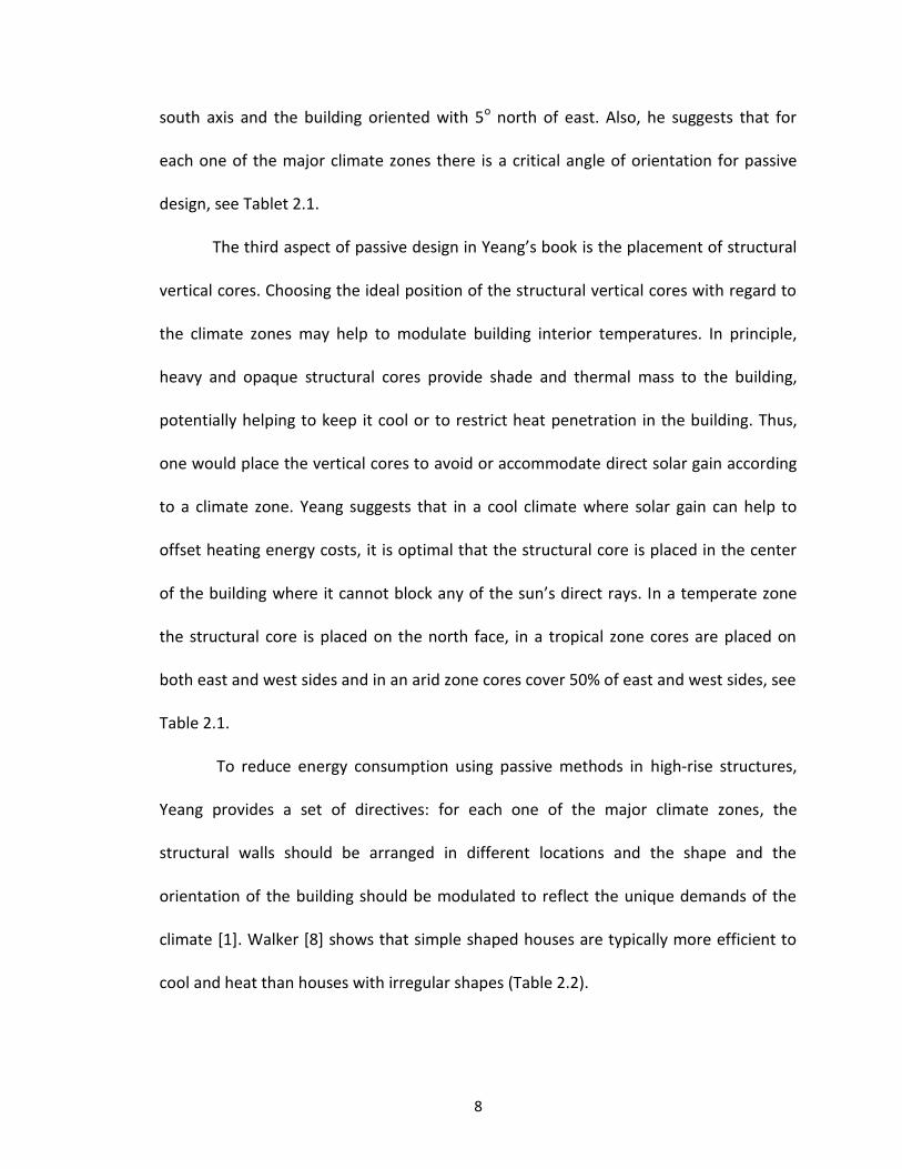
displacement of 0.5 m. Hence, these three major conclusions regarding building

structural performance:

(1) Maximum lateral displacements at the tops were close and comparable. This

will allow precise comparison of the amount of material that is being added because of

RLLS.

(2) In the case of the Sides configuration, because of the shear walls are placed

on the sides, this played a major role in minimizing the torsion displacement. Otherwise,

in the other configurations, the maximum drifts were controlled by the torsion

displacement.

(3) The RLLS effectively reduced the potential torsion displacement in the Edge

configurations, but resulted in larger structural elements that will reflect negatively on

the cost and the embodied energy of the material, as we will see in the calculation of

costs later.

A final observation: we can now calculate the amount of structural material for

BSS and SLLR. Then we will (In the next chapter) calculate the total cost (operational &

82

embodied energies and material) for a 50 year life span, so as to know whether the

tradeoff of placing the structural cores to maximize operating energy efficiency will not

cause the total cost to be too great.

Table 5.2 The lateral displacements result with SLLR

Co

nfi

gura

tio

ns

stiffness eccentricities

(m)

Maximum displacement service wind load Pwx and

0.75 Pwx

Maximum displacement service wind load Pwy and

0.75 Pwy

Serv

icea

bili

ty t

hre

sho

ld (

m)

(ASC

E 7

-10

)

With SLLR - strength checked

With SLLR-serviceability checked

With SLLR - strength checked

With SLLR-serviceability checked

X Y Ux (m) Uy (m)

Sid

es

12.7 3.9 0.87 0.45 0.88 0.46

0.5

Hal

f Si

des

10.1 5.4 0.98 0.44 1.16 0.43*

Edge

9 12 1.24 0.43* 1.36 0.41*

Ce

ntr

al

8 8 1.0 0.44* 1.1 0.45*

Pwx wind loading parallel to x-axis; Pwy wind loading parallel to y-axis. * Deformation due to torsional displacement, See Figure 4

83

All displacements are in meter

Figure ‎5.3 Lateral displacements at the roof (service wind loads Pw and 0.75 Pw)

Pw

y

y

xUy=

0.4

6

y

x

Pwx

Ux=0.45

y

x

0.75

Pw

y

Uy=

0.28

Uy=

0.42

ex

0.75Pwx

Ux=0.36

ey

y

x

Ux=0.31

y

x

Pw

y

Uy=0.28

y

xPwx

Ux=0.44

Uy=0.01

Ux=0.35

Uy=0.01

y

x

0.7

5P

wy

Ux=0.11

Uy=0.43

Ux=0.11

Uy=0.14

y

x

0.75Pwx

Ux=0.35

Uy=0.05

Ux=0.31

Uy=0.05

y

x

Pw

y

Uy=0.36

y

xPwx

Ux=0.06

Uy=0.24

Ux=0.37

Uy=0.24

y

x

Uy=0.41Uy=0.11

0.7

5P

wy

ex

y

x0.75Pwx

Ux=0.3

Uy=0.31

Ux=0.43

Uy=0.31

ey

Pw

y

Uy=0.26y

x

Pwx Ux=0.23

y

x

0.7

5P

wy

Ux=0.27

Uy=0.18

Uy=0.45

y

x

0.75Pwx

Ux=0.16

Uy=28

Ux=0.44

y

x

Loading Case 1 Loading Case2 Sides model

Loading Case 1 Loading Case2 Half Sides model

Loading Case 1 Loading Case2 Edge model Loading Case 1 Loading Case2

Central model

84

CHAPTER 6

MATERIAL USED EMBODIED ENERGY AND TOTAL COSTS (OPERATIONAL, EMBODIED ENERGIES AND MATERIAL USED)

6.1 Material used embodied energy

The energy required to produce the structural elements such as concrete, steel,

wood, etc., has serious environmental and financial consequences. The energy analysis,

therefore, must take into consideration the added cost of embodied energy, which is

the energy consumed by all of the processes associated with the production of a

building. This includes the mining and manufacturing of materials and equipment as well

as the transport of the materials and the administrative functions. Generally, the more

highly processed a material, the higher its embodied energy is.

Materials in their basic form that have lower embodied energy intensities (such

as concrete, bricks and timber) are usually consumed in large quantities. On the other

hand, materials with higher embodied energy content such as steel or even aluminum

are often used in much smaller amounts. As a result, the greatest amount of embodied

energy in a building can be either from low embodied energy materials such as

concrete, or high embodied energy materials such as steel [36].

Moreover, placing the structural cores to improve operating energy efficiency

may compromise the structural performance unintentionally, thereby increasing the

embodied energy of the structure. Council on Tall Buildings and Urban Habitat (CTBUH)

illustrated that the embodied energy normal-weight reinforced concrete with 100Kg

rebar per cubic meter is 2.12 MJ/Kg [37]. According to Lee et al. the embodied energy

85

virgin steel is 35.3 MJ/Kg and 9.5 MJ/Kg for recycled steel [18]: steel sections are made

from 93.3% recycled steel [38], thus the estimated steel sections embodied energy

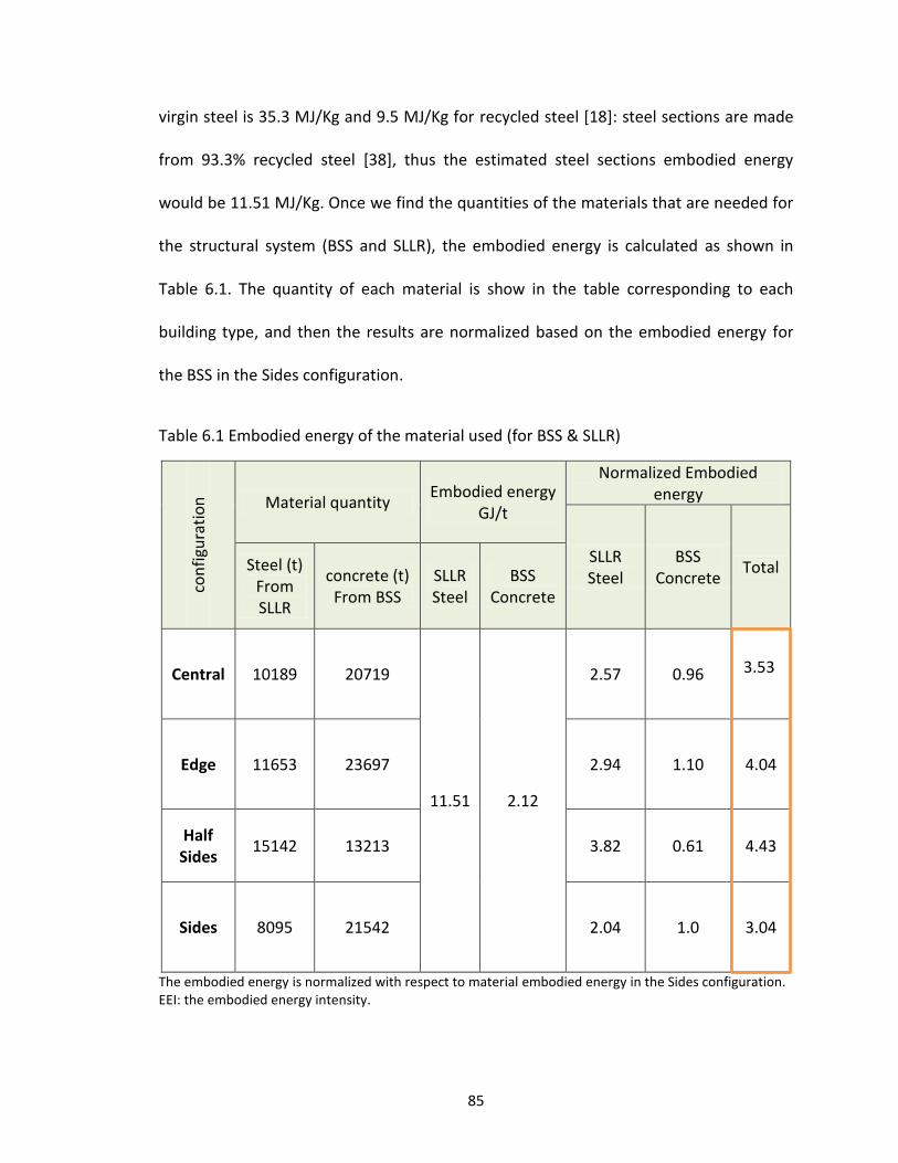
would be 11.51 MJ/Kg. Once we find the quantities of the materials that are needed for

the structural system (BSS and SLLR), the embodied energy is calculated as shown in

Table 6.1. The quantity of each material is show in the table corresponding to each

building type, and then the results are normalized based on the embodied energy for

the BSS in the Sides configuration.

Table 6.1 Embodied energy of the material used (for BSS & SLLR)

con

figu

rati

on

Material quantity Embodied energy

GJ/t

Normalized Embodied energy

SLLR Steel

BSS Concrete

Total Steel (t) From SLLR

concrete (t) From BSS

SLLR Steel

BSS Concrete

Central 10189 20719

11.51 2.12

2.57 0.96

Edge 11653 23697 2.94 1.10 4.04

Half Sides

15142 13213 3.82 0.61 4.43

Sides 8095 21542 2.04 1.0 3.04

The embodied energy is normalized with respect to material embodied energy in the Sides configuration. EEI: the embodied energy intensity.

3.53

86

Table 6.1 illustrates that the highest embodied energy is in the Half Sides

configuration; the reason is because this model accounts for the highest amount of

structural steel for SLLR, which associates with higher unit embodied energy per tonne.

The embodied energy in Edge model is the highest for the BSS and second highest for

SLLR the Central model demanded the lowest total embodied energy after the Sides

model. It is worth noting that the Central model used to be the worst model in terms of

operational energy. This may indicate that it is not necessary that buildings of lower

operational energy will have lower embodied energy or vice versa.

6.1.1 Summary of the material used embodied energy

We obtained for major conclusions regarding material used embodied energy:

1) The higher embodied energy in the Half Sides configuration is because it

needed the highest quantity of structural material for RLLS. This is mainly as a result of

the extreme lack in BSS being adequate to resist the wind loading considered in this

study.

2) Because of the potential irregularity in the rigidity in Edge configuration led to

a relatively high quantity of structural material for RLLS which led to higher embodied

energy in this model comparing to the others.

3) In the case of the Central model, with taking into account that the lack in BSS

and also the impact of the torsion displacement (load Case2) made RLLS element to be

larger, resulting a relatively high quantity of structural material for RLLS, and the high

embodied energy.

87

4) Opposite scenario In the case of the sides, because the placement of BSS

along the short sides led to reduce the impact of the torsion displacement, resulting a

relatively less quantity of structural material for RLLS, and then less embodied energy.

A final observation: placing the structural cores to improve operating energy

efficiency led to compromising the structural performance, thereby increasing the

embodied energy of the structure. The next steps will bring the total cost of energies

(operational and embodied) in addition to materials and then we can compare the

tradeoff between the energy and the structural performance.

6.2 Cost analysis

The changes in global climate, population increase, concerns about the energy

resource, urban infrastructure, and green buildings (which have become essential to

achieve the sustainability) are all reflected on the economy. This is relevant to our study

through the cost of materials for construction as well as operational and embodied

energies. There are numerous costs associated with acquiring, operating, maintaining,

and disposing of a building system. However, in this analysis we will focus only on the

material cost for the structural lateral loads resistance systems (BSS and SLLR) and the

cost for operational (cooling and heating) and embodied energies. Previously, we found

that different building types with different morphologies would associate with various

amounts of structural material and various energy demands; so, obviously, this would

result in variation on the overall cost between these building types.

88

6.2.1 Cost calculation Assumptions

For the purpose of this study, several assumptions are made: 1) the energy used

for cooling and heating is electricity per kilowatt-hour; this cost will be considered as

constant along buildings’ life span. 2) The unit cost of the embodied energy is the same

as the unit cost of the operational energy. 3) All the buildings have a life span of fifty

years.

6.2.2 Cost of operational energy

Based on the energy analysis and the results previously obtained (Table 4.4) we

can estimate the operational energy cost for each building configuration corresponding

to the energy unit price in each location. The price per-kilowatt-hour of the electricity

energy is varying between the states, where it is $0.16 Boston, MA; $0.12 Sacramento,

CA; $0.1 Las Vegas, NV; $0.21 Honolulu, H [39].These differences in unit price have

potential effect on the total energy cost between the regions (states), but this would not

affect the comparison of our interest, because we are comparing the cost for the four

buildings’ configuration in each single city at a time. Table 6.1 illustrates the annual

operational energy and the extreme differences in the cost associated with it.

In all the regions the upper extreme cost difference happens between the

Central configuration and the Sides configuration (the Sides demands is the lowest in

energy demand). On the other hand, the lower cost difference happens always between

the Sides and the Edge configurations. To visualize these differences in the cost for the

life span of 50 years, we estimate how many years we will have financial gain as a result

from the saving if we use these configurations compared to the worst scenario (see

89

Figure 6.1). As can be seen in cool climate the cost of energy that is needed for Central

configuration for a 50 years life span would be sufficient to Sides configuration for the

same life-span period in addition to a period of 16.5 years; or in addition to a period of

11 years and 7 years if we use the Edge and the Half Sides respectively. In case of

temperate climate using Sides configuration will save operational energy cost needed

for 10 years extra if we use the Central configuration, while we can get enough financial

gain for 6 years, and 4 years extra from the saving if we use the Edge and the Half Sides

respectively. On the other hand, in the tropical climate we may say that all models are

close in terms of energy costs for the given life span.

6.2.3 Cost of material used for BSS and SLLR

Input building and construction costs are determined mainly by the cost of

materials, labor, and erection of the building. According to MEPS International, the cost

of steel structural sections are $908/t [40] (metric tonne) whilst the structural concrete

cost is varying in different parts of the country and all over the world. However, for the

Boston region, which represents the cool climate, the costs have been estimated using

national RS Means data [41], where it is $ 640 /m3 of normal weight concrete including

materials, framing, placing, labor, and also including 100 kg rebar. Also, the cost of one

tonne of steel structure materials is $4300 including material, shop fabrication, shop

primer, and bolted connections.

90

Table 6.2 The operational energy extreme differences in annual energy the cost

climate Unit cost $/kWh

Annual operational energy (AOE) Extreme differences

Central Edge Half Sides Sides AOE % Difference

Energy cost Difference ($)

kwh Min Max Min Max

Cool 0.16 8.413E+06 6.884E+06 7.368E+06 6.326E+06 9 33 89,373 334,054

Temperate 0.12 4.956E+06 4.397E+06 4.579E+06 4.132E+06 6 20 31,763 98,935

Arid 0.1 8.638E+06 7.611E+06 8.008E+06 7.350E+06 4 18 26,114 128,742

Tropical 0.21 7.824E+06 7.622E+06 7.746E+06 7.372E+06 3 6 52,528 94,887

Annual operational energy includes only the heating and cooling load

91

Cool Temperate

Arid Tropical

Figure 6.1 Financial comparison of the operational energy cost for a 50 year life span with respect to the Central configuration

50.0

61.1 57.1

66.5

0

10

20

30

40

50

60

70

Central Edge HalfSides

Sides

year

s; 5

0 y

ear

life

sp

an 50.0

56.4 54.1

60.0

0

10

20

30

40

50

60

70

Central Edge HalfSides

Sides

year

s; 5

0 y

ear

life

span

50.0

56.7 53.9

58.8

0

10

20

30

40

50

60

70

Central Edge HalfSides

Sides

year

s; 5

0 y

ear

life

span

50.0 51.3 50.5 53.1

0

10

20

30

40

50

60

70

Central Edge HalfSides

Sides

year

s; 5

0 y

ear

life

sp

an

92

Similarly, we estimated the material cost for the other locations, where in

Sacramento (which represents the temperate climate), the costs are $566 /m3 of normal

concrete and $4100 /t of steel sections; in Las Vegas (which represents the arid climate)

the costs are $547 /m3 of normal concrete and $4240 /t of steel structure; lastly in

Honolulu (which represents the temperate climate) the costs are $702 /m3 of normal

concrete and $4170 /t of steel structure. Once we find the quantities of the materials

that are used to form the structural elements for the BSS and SLLR systems (which are

used to resist lateral loading), a comparison between the normalized costs for the four

models can be made. Accordingly, Figure 6.2 shows material cost index for the BSS and

the cost index for SLLR. The cost is normalized with respect to the BSS material cost in

the Sides configuration.

Figure 6.2 Material cost index BSS and SLLR

7.63

8.72

11.33

6.06

0.96 1.10 0.61

1.00

0.30

2.30

4.30

6.30

8.30

10.30

12.30

Central Edge Half sides Sides

Mat

eria

l co

st in

dex

SLLR BSS

93

As can be seen, the highest added cost is in the Half Sides model; this may be

reasonable because the material cost in BSS is quite low compared to the others. This is

unlike the case of Edge model which demands the highest material cost in BSS. Besides,

it is still costly for the SLLR. This can clearly state that the penalty of the irregularity in

the rigidity in the Edge model is a high material cost, to achieve structural workability

for this configuration. Both the Sides and Central models were close in terms of BSS

cost, but the Side model demands the lowest cost for SLLR. Total cost index is

illustrated in Table 6.3. As we have found, the worst scenario in terms of the operational

energy cost was the Central configuration. However it becomes the second best to the

Sides model in terms of material cost (BSS and SLLR). The Edge configuration becomes

third and the worst is the Half Sides.

Table 6.3 Total material used cost index

configuration

Material quantities Normalized cost

Steel (t) From SLLR

concrete (m3) From BSS

Total material (BSS+SLLR)

Central 10189 8633 1.22

Edge 11653 9874 1.39

Half Sides 15142 5505 1.69

Sides 8095 8976 1.0

The cost is normalized with respect to material cost in the Sides configuration.

94

6.3 Total cost: Operational, Embodied energies and Material costs

Table 5 shows the results of the summation of total operational, embodied

energies and material costs for fifty years life span. In the case of the cool climate, total

cost of the Half sides model is more than that in other each Individual model, while the

Sides came in rank one, the Edge second, and Central third. Note here that the high

operational energy cost in the Central model is reflected in the total cost; similarly, the

high material cost made the Half Sides model the most costly.

In the second row, temperate climate, the difference between the four models

in the total cost goes down a bit than it does in the cool climate. The Sides model has

the lowest total cost of all the models, while the Central model moved from third

position (in cool climate) to the second rank in this climate. The Half Sides model

remains the most costly in this climate as well. Similarly we note the behavior of the

total cost in the arid climate with a slightly higher cost.

In the case of the tropical climate, the Sides model remains the best, the Central

model deserves second, the Edge third, and the Half Sides fourth. We note here (in this

climate) that the total cost for each individual model is the largest compared with other

regions; the reason is because the unit cost of the electricity energy is high in this

climate, so its affect continues to appear in the total cost.

As previously, to visualize the difference in the cost for the life span of 50 years,

we estimate how many years will have financial gain using these configurations

comparing to the total cost in the Central configurations, see Figure 6.3. As can be seen

in the cool climate, the total cost that is needed for Central configuration of 50 life-

95

spans would be sufficient to the Sides configuration for the same life-span period in

addition to a period of 13.5 years; it would be in addition to 1.7 years if we use the Edge

configuration. On the other hand, the total cost that is needed for Central configuration

of 50 life-spans would be sufficient to Half Sides configuration only for 43.5 years, which

means we need more finance to operate the Half Sides than the finance needed for the

Central configuration.

In case of the temperate and arid climate zones, using the Sides configuration

will save cost for about 10 years extra than if we use the Central configuration.

Oppositely, we will need more finance if we use the Edge and the Half Sides compared

to the Central configuration. The case of the tropical climate is similar but the cost

saving between best configuration (Sides) and the second option (Central) gives 5.8

years extra if we use the best configuration. Otherwise, the other two configurations

(Edge and the Half Sides) do not make it for a 50 years life span.

6.3.1 Summary of the cost estimating

We obtained four major conclusions regarding cost estimating:

1) The results obtained for all individual cost estimating (operational energy ,

embodied energy, and material used) suggest that serious financial saving can be

achieved as soon as the adoption of the Sides configuration takes place in all climate

zones.

96

96

Table 6.4 Summation all costs operational, embodied energies and material for fifty years life span

97

Cool Temperate

Arid Tropical

Figure 6.3 Financial comparison of the total cost for a 50 years life span with respect to the Central configuration

50.0 51.7

45.3

63.6

0

10

20

30

40

50

60

70

Central Edge HalfSides

Sides

year

s; 5

0 y

ear

life

sp

an 50.0

47.6

41.1

60.4

0.0

10.0

20.0

30.0

40.0

50.0

60.0

70.0

Central Edge HalfSides

Sides

year

s; 5

0 y

ear

life

span

50.0 48.8

42.3

59.9

0

10

20

30

40

50

60

70

Central Edge HalfSides

Sides

year

s; 5

0 y

ear

life

span

50.0 47.9

43.7

55.8

0

10

20

30

40

50

60

70

Central Edge HalfSides

Sides

year

s; 5

0 y

ear

life

sp

an

98

2) The statue of the morphology in the Edge configuration gave him a good

opportunity (the second rank for all climate zones) to conserve energy consumption, but

the tradeoff was too great for both the structural performance and the material used

and embodied energy. The main reason was because the potential irregularity in the

rigidity caused substantial materials cost, which is reflected negatively on the final cost.

3) Unlike the scenario with the Central configuration, the state of the

morphology gave him the worst case in terms of the energy consumption, but when we

add up all costs for the 50 year life span, this model become the lowest cost after the

Sides model for the temperate, arid, and tropical climate zones, while barely in the cool

climate.

An observation: in the case of the Central configuration we can obtain a

significant reduction on the total cost through the given ability to improve its energy

performance (see section 4.4 and Appendix B).

Placing the structural cores and the manipulation with the building morphology

to improve operating energy efficiency sometimes is wise approach (as in the case of

the Sides configuration), but in other times the tradeoff for the structural performance

too expansive (like in the case of the Sides configuration).

99

CHAPTER 7

SENSITIVITY OF ENERGY DEMAND TO BUILDING FOOTPRINT ASPECT RATIO AND BUILDING ORIENTATION

7.1 Introduction

Global warming and climate change are major challenges facing the nation and

the world. More than two thirds of the electricity energy and one third of the total

energy in the US are used to heat, cool, and operate buildings [42], representing roughly

18% of all U.S. CO2 emissions in that year. A reduction in building energy consumption

will help to mitigate the energy security and climate change impacts of buildings. The

reduction in energy use may translate to a financial savings that can be achieved

through the development of new technologies (for the building's envelope, mechanical,

and lighting systems) that save energy and reduce CO2 emissions. The benefit to the

building owner is lower monthly utility expanses, and smaller less expensive HVAC

equipment. Building energy codes are intended to promote energy efficiency by

specifying minimum material, mechanical and construction standards [43].

An alternative approach is the use of passive systems that employ renewable

energy sources. Passive systems avoid the need for heating or cooling through better

design, construction, and operation. They utilize solar or wind energy to heat, cool, or

light buildings.

Therefore, in this chapter we analyze the sensitivity of energy demand to two

parameters of passive design related to building layout and site. The key parameters we

investigate are building footprint aspect ratio and the building orientation that have

100

been considered important factors in passive design [1]. Four high-rise office buildings

(glazed curtain wall) with four different aspect ratios (1:1, 1:2, 1:3, and 1:4) are

thermally analyzed in four climate zones: cool, temperate, arid, and tropical. Energy

demand is calculated for each model with respect to two opposing orientations

(Figure7.1). The four high-rise buildings are modeled to meet International Energy

Conservation Code (IECC) 2009 requirements, which reference several American Society

of Heating, Refrigeration, and Air Conditioning Engineers (ASHRAE) standards, including

Std. 90.1 for commercial building construction [6].

In the following sections we describe the analytical method and the primary

variables that will be measured against energy use in the four modeled buildings. We

then summarize the results for each of the thirty-six scenarios and present the

conclusion.

7.2 Building Materials and Method

Four models of high-rise office buildings are considered in this study to evaluate

the sensitivity of energy demands to variations in: (1) footprint aspect ratio (1:1, 1:2,

1:3, and 1:4), and (2) building orientation. Since our goal is to isolate the influence of

building site layout planning on energy demand, all other buildings descriptors such as

the square footage, number of stories, building height, and occupancy for the four

buildings are held constant across all four buildings. Specifically, we treat the thermostat

range, internal design conditions, occupancy, infiltration rate, and hours of operation as

fixed control variables (Table 4.3). The four buildings are 200 meters in height, 50 stories

101

that are 4.0 m floor-to-floor height, with a total conditioned floor area of 135,000

square meters.

The primary material for the envelope is a glazed curtain wall, which comprises

of double pane standard glass with 10% metal framing. The floors are composed of

layers of 10mm ceramic tiles, 5mm screed, 100 mm normal concrete, insulation (as

needed to meet the R-value specified for a climate according IECC 2009), 50 mm air gap,

and 10 mm plaster underneath (see Table 4.1).

To simplify the thermal analysis, we have neglected the effect of surrounding

buildings, in essence assuming that the buildings are erected on flat open ground and

are aligned with the cardinal directions.

Figure 7.1 Building orientation considered in this study

The four buildings are simulated in each of the four major climate zones and as

previous we have selected specific cities to represent each climate zone: Boston,

Massachusetts for the cool zone, Sacramento, California for the temperate zone, Las

N

ϴ=90

ϴ=0; N-S Orientation ϴ=90; E-W Orientation

102

Vegas, Nevada for the arid zone, and Honolulu, Hawaii for the tropical zone. Building

envelope materials are selected for all four models to meet the requirements of thermal

properties of IECC 2009, corresponding to each climate zone.

7.3 Analytical Approach:

Auto esk’s Ecotect energ si ulation package was used for the thermal analysis.

As previous the building geometry was prepared in Revit 2010, and then imported as

surfaces and rooms to Ecotect 2011. In Ecotect, thermal properties are assigned to the

envelope. The basic material of an element (floor, roof, glazing wall, etc.) is assigned

first, the thermal properties of element and the insulation is then applied according to

specifications of IECC 2009. The next step is to assign a weather file that corresponds to

the climatic zones selected for this study and to provide occupancy and scheduled usage

data. Finally, the program calculates monthly and annual heating and cooling loads

according to the prescribed conditions.

7.3.1 Thermal analysis

The thermal analysis involves examining each of the four models (1:1, 1:2, 1:3, and 1:4)

in each of the four climatic zones (cool, temperate, arid, and tropical). For each climate

zone, weather data (TMY files) for each city is loaded and the four models are tested

under equivalent interior thermal and schedule conditions. That is, the only differences

among the four runs in the same climate zone are the building width to length ratio

(aspect ratio) for one orientation at a time.

103

Figure 7.2 Building plan view and envelope thermal properties

Ecotect calculates the overall heat gain/loss; and then with choose the way the

comfort zone is calculated for each day of the year. We use the Flat Comfort Bands method,

which sets upper and lower limits for comfort temperatures. If the internal zone

73.50 m

36

.75

m

x

y

Plan view 1:2 configuration

23 m28 m

18.4

m 20 m 12

.5 m

15.6 m

90 m

x

y

Plan view 1:3 configuration

15 m 24 m 1

2 m

19 m28 m 34 m

30

m

x

Elevation

50

@ 4

m

103.85 m

x

y

Plan view 1:4 configuration

13 m

23 m

9 m

18 m35 m 43 m

26

m

51

.96

m

51.96 m

Plan view 1:1 configuration

y

18 m

25 m

17 m

22

m

x

21 m14 m

Glazing walls

Partitions

0.0 18 m 36 m 54 m 72 m

104

temperature is either above or below the temperature limits for the prescribed comfort

zone, then thermal environmental conditions are unacceptable to a majority of the

occupants within that space. Factors that determine thermal environmental conditions

are temperature, thermal radiation, humidity, air speed, and personal factors such as

activity and clothing. Environmental factors are influenced by: 1) Direct solar gain, or

radiant flow through transparent surfaces; 2) Internal (sensible) heat gain from lights,

people, and equipment; 3) Conductive heat flow through opaque (envelope) elements;

4) Radiant flow through opaque (envelope) elements; 5) Ventilation and infiltration heat

flow through cracks and openings; 6) Inter-zonal heat flow between adjacent zones,

which for this analysis is negligible. Conductive and radiant flows through opaque

ele ents are treate together an escribe as “Fabric” in Ecotect. Personal factors

such as activity (metabolic rate) and clothing (insulation of clothing) are treated as

constant for all building occupants.

In this study there are two main stages of the thermal analysis. The first stage is

to find the sensitivity of the energy demand (heating and cooling loads) to the change of

the surface area ratio (SAR), which relates to floor-plan aspect ratio:

This analysis consists of thirty-two different simulation runs (of four models in two

orientations in four climate zones = 4×2×4), where annual cooling and heating loads are

calculated for each model. The results corresponding to the N-S orientation are

provided in Table 7.1; and the difference in the total energy demand between the N-S

and E-W orientations is not significant, as shown in Figure 7.3. Using the model of 1:4

105

aspect ratio as an example, the monthly and yearly energy demand ratios (EDR) for each

of the four climate zones are shown in Table 7.2.

Also the passive solar heat gain ratio (PSHGR) of the model of 1:4 aspect ratio is

displayed in Figure 7.4. Moreover, the total heat gain and heat gain ratio (HGR) of the

month of July are broken down into individual sources of direct (solar) gain, internal

gain, fabric, and ventilation. Table 7.3 presents the percentage of each of these heat

sources and how they vary by orientation. The total energy demand for each orientation

are not significantly different, even though the E-W oriented models have a much higher

potential for passive solar heat gain.

The next stage of the thermal analysis investigates why the differences in the

energy demand are negligible. One possible reason maybe is because of the thermal

properties of the IECC 2009 envelope. In the initial analysis, the glazing walls were

modeled with U-factors and SHGC set according to the regional climate. These walls

were subsequently modeled using single-pane glazing, which has inferior thermal

properties (U=6.0 W/m2K & SHGC=0.94). The simulation was run again to evaluate the

total energy demand for each of the two orientations. The results of the new simulation

runs show that buildings oriented E-W require 12% more energy than those oriented N-

S, and that the passive solar heat gain in July is significantly increased.

106

7.3.2 Demand sensitivit glazing walls built to code

For each building in the climate zones of Cool, Temperate, and Arid, the change in

energy demand is slightly significant, where by increasing the surface area (up to 20%),

energy demand is increased by 5.1-7.9% (table 7.1) depending on the climate zone. In

the tropical climate, however, the energy demand is insensitive to the variations in SAR,

where the average increment percent is 0.4% and the total increase is 0.84%.

Of course, an increase in the surface area (SAR) is likely to lead to an increase in

the materials used, may impact construction costs and embodied energy. Furthermore,

increases in the surface area may result in an increase in the area exposed to wind

pressure, which might lead to the need of a larger size of structural element, which also

impact construction costs and embodied energy.

The differences in the total energy demand for two building orientations (N-S &

E-W) in each climate zone are nearly negligible (see Figure 7.3). The horizontal axis

represents the SAR correspon ing to the four buil ing’s aspect ratios (1:1, 1:2, 1: , an

1:4), while the vertical axis represent EUI.

These small differences in EUI raise questions about the results presented in

Figure 7.4, where the monthly breakdown shows solar heat gains and losses resulting

from building oriented E-W are much greater than if the building were oriented N-S. The

sources of total energy demand for the month of July are presented in Table 7.3, and it

is clear that the influence of solar loads is small compared to internal, fabric, or

ventilation loads.

107

10

7

Table 7.1 Energy demand verses SAR (N-S orientation)

Width to length ratio - increase in SAR

T pe

Climate

1:1 1:2 1:3 1:4

Heating Cooling EUI Heating Cooling EUI Heating Cooling EUI Heating Cooling EUI

kwh/ 2 kwh/

2 kwh/ 2 kwh/ 2

Cool 49.8 9.4 59.2 51.9 9 60.9 53.6 8.7 62.3 55.9 8.4 64.3

Temperate 7.9 30.7 38.55 8.4 30.7 39.1 8.9 30.8 39.8 9.7 31 40.6

Arid 5.8 57 62.8 6.1 57.9 64.0 6.5 59 65.5 7 60.4 67.4

Tropical 0.0 62.5 62.5 0.0 62.75 62.6 0.0 63.4 63.4 0.0 64.1 64.1

EUI: Energy Use Intensity

108

Cool

Temperate

(Continue)

37.00

42.00

47.00

52.00

57.00

62.00

67.00

72.00

0.30 0.32 0.34 0.36 0.38 0.40

EUI k

wh

/m2

Surface area ratio

ϴ=0 ϴ=90 1.2 %

37.00

42.00

47.00

52.00

57.00

62.00

67.00

72.00

0.30 0.32 0.34 0.36 0.38 0.40

EUI k

wh

/m2

Surface area ratio

ϴ=0 ϴ=90

2.2 %

109

Arid

Tropical

Figure 7.3 Sensitivity of EUI to the change in surface area ratio

37.00

42.00

47.00

52.00

57.00

62.00

67.00

72.00

0.30 0.32 0.34 0.36 0.38 0.40

EUI k

wh

/m2

Surface area ratio

ϴ=0 ϴ=90 2.3%

37.00

42.00

47.00

52.00

57.00

62.00

67.00

72.00

0.30 0.32 0.34 0.36 0.38 0.40

EUI k

wh

/m2

Surface area ratio

ϴ=0 ϴ=90 3.1%

110

The amount of heat gain from passive sources represents 5-20% of the total heat gain.

This is consistent for both orientations, and the effect is trivial compared to the total

heat gain.

7.3.3 Demand sensitivity with non-code-compliant glazing on walls.

The second stage of thermal analysis is an investigation of the sensitivity of built-

to-code glazing systems on passive solar heat gain, compared to single-pane glazing,

which has poorer thermal properties. The outcome demonstrates that code

requirements for glazing systems results in reductions in direct heat gain to become

represent 5% rather than 24% of total heat gain(N-S),while become represent 8% rather

than 34% of total heat gain(E-W), (Table 3 & Table 5 for arid climate). Code-built glazing

also reduces total energy demand by 12%, which also explains why there is such a small

effect from varying building orientation on monthly and yearly energy demand.

111

Table ‎7.2 Energy demand ratio, EDR, (model of 1:4 aspect ratio)

Months

Energy demand ratio (EDR)

Cool Template Arid Tropical

Jan 1.01 1.01 1.03 0.96

Feb 1.01 1.02 0.97 0.99

Mar 1.01 0.99 0.99 1.05

Apr 0.99 1.02 1.04 1.07

May 0.97 1.04 1.05 1.06

Jun 0.99 1.04 1.03 1.05

Jul 1.011 1.034 1.026 1.055

Aug 1.02 1.02 1.02 1.05

Sep 1.00 0.99 1.01 1.03

Oct 1.01 0.98 0.99 1.01

Nov 1.02 1.00 0.99 0.99

Dec 1.02 1.02 1.03 0.97

yearly 1.01 1.02 1.02 1.03

112

11

2

Figure 7.4 Monthly passive solar heat gain ratio (model of 1:4 aspect ratio)

JAN FEB MAR APR MAY JUN JUL AUG SEP OCT NOV DEC

Cool 0.76 0.86 0.95 1.05 1.15 1.15 1.16 1.13 0.99 0.90 0.80 0.72

Temperate 0.80 0.90 0.99 1.17 1.31 1.42 1.40 1.27 1.04 0.90 0.80 0.77

Arid 0.81 0.91 1.04 1.27 1.44 1.53 1.51 1.37 1.13 0.95 0.82 0.77

Tropical 0.94 1.02 1.19 1.42 1.49 1.45 1.49 1.56 1.33 1.11 0.98 0.91

0.00

0.20

0.40

0.60

0.80

1.00

1.20

1.40

1.60

1.80

pas

sive

so

lar

he

at g

ain

rat

io p

assi

ve s

ola

r h

eat

gai

n r

atio

(P

SHG

R)

Months

Cool Temperate Arid Tropical

113

11

3

Table ‎7.3 Sources of heat gain (Wh) in July- built to code envelope (model of 1:4 aspect ratio)

Climate Cool Temperate

Orientation ϴ=0 ϴ=90 July HGR

ϴ=0 ϴ=90 July HGR

Direct 1.1E+08 17% 1.3E+08 20% 1.16 1.1E+08 8% 1.5E+08 11% 1.40

Internal 5.1E+08 78% 5.1E+08 75% 1.00 5.1E+08 40% 5.1E+08 38% 1.00

Fabric 2.1E+07 3% 2.3E+07 3% 1.11 2.8E+08 22% 2.9E+08 22% 1.02

Ventilation 1.3E+07 2% 1.3E+07 2% 1.00 3.8E+08 30% 3.8E+08 29% 1.00

Total 6.573E+08 6.783E+08 1.032 1.277E+09 1.325E+09 1.038

Climate Arid Tropical

Orientation ϴ=0 ϴ=90 July HGR

ϴ=0 ϴ=90 July HGR

Direct 1.1E+08 5% 1.6E+08 8% 1.51 9.9E+07 10% 1.5E+08 14% 1.49

Internal 5.1E+08 25% 5.1E+08 24% 1.00 5.1E+08 50% 5.1E+08 47% 1.00

Fabric 6.1E+08 30% 6.2E+08 29% 1.01 2.2E+08 21% 2.3E+08 21% 1.05

Ventilation 8.3E+08 40% 8.3E+08 39% 1.00 2.0E+08 19% 2.0E+08 18% 1.00

Total 2.068E+09 2.129E+09 1.03 1.029E+09 1.087E+09 1.057

114

Table ‎7.4 Breakdown heat gain (Wh) in July in Arid climate – regular glass envelope (model of 1:4 aspect ratio)

Heat gain (Wh) July HGR

ϴ=0 ϴ=90

Direct 7.4E+08 24% 1.2E+09 34% 1.62

Internal 5.1E+08 16% 5.1E+08 14% 1.00

Fabric 1.0E+09 33% 1.0E+09 29% 1.01

Ventilation 8.3E+08 27% 8.3E+08 23% 1.00

Total 3.099E+09 3.564E+09 1.15

7.3.4 Summary of results

B si ulating each buil ing configuration using Auto esk’s Ecotect, we can raw

two major conclusions regarding building energy demand:

(1) For the buildings in Cool, Arid, and Temperate climate zones, the energy demand

may be considered marginally sensitive to changes in surface area ratio (SAR). Increasing

the envelope surface area by 20% leads to energy demand increases of 5.1-7.9%

depending on the climate zone. The energy demand for buildings in the Tropical climate

zone is insensitive to variations in SAR.

(2) The energy performance of high-rise office buildings is not sensitive to the

passive solar gain as long as the exterior envelopes are built to IECC 2009 requirements

for thermal performance.

115

CHAPTER 8

CONCLUSIONS AND RECOMMENDATIONS AND FUTURE WORK

8.1 Conclusions

The energy performance of a high-rise office building is highly impacted by its

morphology. This study proves that building configuration (footprint shape and the

placement of structural vertical core/walls) significantly influences overall energy

performance. Furthermore, placement of the structural vertical core/walls in the east

and west sides and building footprints with an aspect ratio of 1:3 (Sides configuration)

lead to significant reduction in the energy demand in the four major climatic zones.

Significant improvements in energy performance can be gained by adding

opaque surfaces in the Central configuration envelope (thermal analyses EPO and EDO).

Moreover, envelopes with more opaque surfaces increase the opportunity for placing

the structural elements so as to avoid the asymmetrical distribution, which would lead

to improving the structural performance without compromising energy performance.

It is often noted that the thermal mass contributes to reductions in building

energy consumption, and concrete materials have good thermal mass properties.

However, in this study, we do not obtain the expected result of improving the energy

performance (where increasing thermal mass material by 100%, the energy demand

changed by around 0.5%) by increasing the amount of thermal mass in the building

envelope.

In the case of the sides configuration placing the structural cores to improve the

operating energy efficiency works well without compromising the structural

116

performance; it is desirable to be in that place, because the placement of the shear wall

along the short sides leads to reduce the impact of the torsion displacement, resulting in

relatively less quantity of structural material, and then less embodied energy and cost.

The state of the morphology in the Edge configuration gave it a good

opportunity (the second rank for all climate zones) to conserve energy consumption, but

the tradeoff was too great for both the structural performance and the material used

embodied energy. The main reason was because the potential irregularity in the rigidity,

which caused a substantial growth in materials cost that reflected negatively on the final

cost.

Finally, high quality thermal properties of code-built envelope systems offer

more flexibility to designers with regard to the building site planning (geometry, layout,

and orientation) without creating negative impacts on total energy demand. On the

other hand, this limits the possibility of maximizing the advantages of passive heat gain.

And, because built to code buildings are not significantly sensitive to direct solar gain, it

leaves little room for other passive design strategies for energy conservation such as

shading devices, landscaping, and thermal mass.

8.2 Recommendations

As we have found, in the case of the Central configuration, adding opaque

surfaces to the East-West sides significantly improves energy performance. Our

recommendation is to consider these opaque surfaces as shear walls to optimize

structural performance.

117

As mentioned, thermal mass is generally thought to be a good way to reduce

overall energy demand, though our study indicates otherwise. Our recommendation is

to investigate new opportunities to take advantage of the presence of the thermal mass.

We can start by investigating the effective thickness, investigating the effect of the

insulation on the thermal mass, and investigating the relationship between the thermal

mass exposed surface and the insolation, etc.

Making good use of natural light reduces the need of artificial lighting and helps

provide a feeling of well-being to office workers. Buildings are lit by a combination of

daylight entering through windows and skylights and electric-light sources. Maximizing

the use of natural light is a very important element in the sustainable design. One of the

objectives of the envelope with glazed curtain walls is to use the natural lighting. Also, in

some cases the shape of the building is designed so natural daylight reduces the need

for artificial lighting. Therefore, our recommendation is to include the effect of natural

lighting on the energy demand for the given buildings’ morphologies.

8.3 Future work

Based on the conclusions, positioning the opaque surfaces on the East-West sides

significantly improves energy performance for two building configurations (the Sides

and the Central), and also the placement of these opaque surfaces made for the

structural purposes is highly desirable (to reduce torsional displacement under lateral

loading).

Thus, the first future work would focus on optimizing each of these configurations

(the Sides, the Central) for each of the four climate zones. This optimizing should

118

consider energy and structural performances, trade-off between the cost of the high

performance envelope versus the increased the energy performance.

Second future work would find out how the structural performance of these two

configurations would change, if the building height is increased and how this affects the

total cost (energy and material) for a given building life span.

Third future work would include a finance comparison between use insulation

material and use of thermal mass, which inherently have a good characteristic of

thermal insulation; taking into account the embodied energy for both the insulation and

thermal mass materials.

Lastly, investigate how the energy demand would change if the system type is

Mixed-Mode System (rather than a full Air-conditioning system), which is a combination

of air-conditioning and natural ventilation. This investigation may require changes in the

building morphologies for natural ventilation; the latter may possibly affect the building

structural performance.

119

APPENDIX A

PRELIMINARY ANALYSIS

A.1 Preliminary structural walls analysis

A preliminary investigation is made to find out for each model what height the

current lateral resistance systems can likely withstand under the wind loads. The

approach here is to calculate the maximum bending and torsion stresses and the

maximum disablement on the walls, and then compare them with the limits. The limits

here are maximum bending stress is , where

is the compressive strength for

normal weight concrete(28 Mpa), displacement

[29], where Δ is the lateral

drift, and h is the wall height, and maximum torsion stress is √ . Based on ASCE

7-10, wind loads have been calculated for each model (Sides, Edge, Half Sides, and

Central).

A.1.1 Wind Loading: Calculation Example

Sides model use here as calculation example that illustrates the procedure for

calculating the wind load. Plan view and the building elevation are shown below .Based

on the expression in ASCE 7-10 Eq. (27.3-1) the velocity pressure is given by.

Where qz is the velocity pressure, V is the basic wind speed at 10m height, kd is the

directionality factor, kzt is the topographic factor, and kz is the exposure coefficient.

Based on Tables 1.5-1, 26.6-1, and Figures 26.5-1A, 26.8-1 in ASCE 7-10 the parameters

are assigned values of: kzt =1; kd=1; and for risk category II the basic wind speed V=58

120

m/s (130 mi/h), Boston region. The exposure coefficient (according to Table 27.3-1 in

ASCE 7-10) given by.

Sides model plan view and elevation

...................(A.2,a)

...................(A.3,b)

Where α is the power law coefficient, g is the nominal height of boundary layer; from

the Table C26.7-12 in ASCE 7-10 the parameters are assigned values of: α= .0 ; g=366.

Given all these values for the velocity pressure parameters, the wind pressure is.

At this point the velocity pressure is determined; now calculate the design wind load,

which is based on the expression (ASCE 7-10 Eq. (27.4-1)).

( )

50

@ 4

m

200

m

90 m

Elevation

90 m

30

m

Plan view(sides model)

0.45 m

Wind

121

Where P is the design wind pressure, G is the gust effect factor, Cp is the external

pressure coefficient, qh is the velocity pressure evaluated at height z = h, and GCpi is the

topographic factor. Based on Tables 26.11-1, and Figure 27.4-1, in ASCE 7-10 the

parameters are assigned values of: ; Cp = 0.8 in windward wall, -0.5 in

leeward wall, and -0.7 in sides walls. The gust effect factor assumed to be G=0.92. Given

these values for the design wind pressure parameters:

The figure below shows the pressure loading that are obtained from Eq.(A.6) with using

the calculated values of by Eq.(4.8). So the lateral- force resistance system must

resist this loading, which wind blows on the front or rear of the building.

A.1.2 Stresses and Displacement: Calculation Example

We assumed the wind load has a trapezoidal distribution. Based on beam theory

approach the maximum bending stress can be calculated by flowing equation:

Where σ is the bending stress, M is the maximum bending moment at the base, I is the

moment of inertia of the wall cross section, and C is the perpendicular distance from

compressive face to the neutral axis. The torsional stress is calculated as:

0.97 kn/m2

122

Wind pressure on the building surfaces

Where T is the twisting moment per unit height acting about a vertical axis of the

building. This twisting moment results from the eccentricity (e), which is assumed to be

the perpendicular distance between the center of pressure of the wind load Pw and the

center of rigidity (c.r) of the shear walls in floor plan.

.....(A.9)..................................................PeT w

Calculating the lateral displacement at the free end, by using the following equation:

0.0 m

100 m

15 m

200 m

3.19 kn/m2 1.62 kn/m2

1.85 kn/m2

2.73 kn/m2

123

Where Δ is the displacement at the free end, Ec is the normal weight concrete modulus

of elasticity, h is the wall height, is the wind load at point a, is the wind load at

point b.

Following the same steps for each model the stresses and displacements in the

strongest direction of the building were calculated. The results were as following: for

the Central configuration, the BSS is adequate for a height of up to 96 m with the wind

load perpendicular on Y direction, or up to 76 m with the wind load on orthogonal

direction. In the case of the Sides configuration, the BSS is adequate up to 100 m with

the wind load perpendicular on X. In the case of the Half Sides configuration, the BSS is

adequate up to 76 m with the wind load perpendicular on X. In the case of the Edge

configuration, the BSS is not adequate, because of the substantially torsional stress.

A.1.2 The eccentricity e for flexible structures

Loading in Case2 is taking into account the presence of the eccentricity e (ex. ey) for the

x, y principal axis of the structure, respectively. This eccentricity is calculated based on

the equation 27.4-5, ASCE 7-10 as following:

√

√

124

where as it is determined for rigid structures where in (m); in (m) is

the distance between the elastic shear center and center of mass of each floor; is

taken as 3.4.

√

(

)

⁄

Wind load: (a) Actual load distribution; (b) Trapezoidal distribution

Where where is the intensity of turbulence at height where is the equivalent

height of the structure defined as , but not less than for all building

12

7 k

n/m

1

87

kn

/m

12

7 k

n/m

18

7 k

n/m

125

heights . and are constants depend on the exposure (see table below); is the

background response is given by

√

[

]

where is the height of other structure in (m); is the integral length scale of

turbulence at the equivalent height given by:

(

)

where and are constants listed in table below.

√

⁄

Terrain exposure B constants (ASCE 7-10)

(m) c (m)

Exposure B 97.54 1/3 0.3 1/4 9.14 0.45

where mean hourly wind speed at height in (m/s); is the basic wind speed in in

(m/s); is the damping ratio; and are constants as listed.

126

where in (m). Based on these equations, the critical cases of the eccentricities as listed

for the x, y principal axis corresponding to each configuration, e (8, 8) for the Central

model; (9, -13) for the Edge model; (10.14, 4.83) for the Half Sides model; and e(12.72,

3.9) for the Sides model.

A.1.3 Shear wall thickness determination

Assuming the wall thickness change about each 12-story. Based on the flexural strength,

we may estimate the preliminary thickness of the shear wall along its height.

127

where Mu is the external moment due to external loading; Mn is the nominal moment

(design resisting moment at section); Φ is the strength reduction factor. Mn can be

calculated as following [44]:

(

) (

)

Where As is the total area of vertical reinforcement at section (in2); fy specified yield

strength of vertical reinforcement (psi); Lw is the horizontal length of the shear wall

(in);Nu is the axial load (Ib).C is the distance from the extreme compression fiber to the

neutral axis (in); =0.85 for concrete strength up to 4000 psi.

A.1.3.1 Calculation example

Given the result analysis for the Sides model (For Mu and Nu); Lw=98.4 ft. ; =4 ksi; fy=

60 ksi; =0.85; ; Note the gravity loads are included wall self-weight 390 kip/ft,

dead load 52.63 psf, and live load 65.16 psf. Note the dead and the live loads are in each

floor on tributary area of 1210 ft2.

128

To start assume wall thickness at the base is h1 = 2.952 Ft. (0.90 m)

Nu=31451 kip

(

)

(

)

As=1349 in2 (1100 #10)

S=2.21 in

Hence, use h1= 2.952 Ft. (0.90 m)

Mu= 2463309 kip.Ft

Now assume wall thickness h2 = 2.624 Ft. (0.80 m)

Nu=23660 kip

(

)

(

)

As=894.16 in2 (900 #9)

S=2.7 in

Hence, use h2= 2.624 Ft. (0.80 m)

Mu= 1969868 kip.Ft

129

Now assume wall thickness h3 = 2.296 Ft. (0.70 m)

Nu=15725kip

(

)

(

)

As=138 in2 (450 #5)

S=5.35 in

Hence, use h3= 2.296 Ft. (0.70 m)

Mu= 652703 kip.Ft

finally assume wall thickness h4 = 1.968 Ft. (0.60 m)

Nu=7934kip

(

)

(

)

As=76.66 in2 (250 #5)

S=9.6 in

Hence, use h3= 2.296 Ft. (0.60 m)

Mu= 181477 kip.Ft

130

External forces (Sides Model)

Vu=31400 kn

Nu=139893 kn

Mu=3340000

kn.m

Vu=25004 kn

Nu=105239 kn

Mu=2670944

kn.m

Vu=17200 kn

Nu=69947 kn

Mu=885000

kn.m

Vu=9334 kn

Nu=35292 kn

Mu=246064

kn.m

48 m

100 m

148 m

200 m

h1

h2

h3

h4

12

7 k

n/m

18

7 k

n/m

131

APPENDIX B

COST INDEX

Cool Temperate

Arid Tropical

Operational cost index based on the cost normalization with respect to the cost in the

Sides model

1.33

1.09 1.16

1.00

0.00

0.20

0.40

0.60

0.80

1.00

1.20

1.40

Central Edge HalfSides

Sides

Co

st in

de

x

1.20

1.06 1.11 1.00

0.00

0.20

0.40

0.60

0.80

1.00

1.20

1.40

Central Edge HalfSides

Sides

Co

st in

de

x

1.18

1.04 1.09

1.00

0.00

0.20

0.40

0.60

0.80

1.00

1.20

1.40

Central Edge HalfSides

Sides

Co

st in

de

x

1.06 1.03 1.05 1.00

0.00

0.20

0.40

0.60

0.80

1.00

1.20

1.40

Central Edge HalfSides

Sides

Co

st in

de

x

132

Cool Temperate

Arid Tropical

Total cost index (Operational and Embodied energies and Material used) based on the

cost normalization with respect to the cost in the Sides model

1.27 1.23

1.40

1.00

0.00

0.20

0.40

0.60

0.80

1.00

1.20

1.40

1.60

Central Edge HalfSides

Sides

Co

st in

dex

1.21 1.27

1.47

1.00

0.00

0.20

0.40

0.60

0.80

1.00

1.20

1.40

1.60

Central Edge HalfSides

Sides

Co

st in

de

x

1.20 1.23

1.41

1.00

0.00

0.20

0.40

0.60

0.80

1.00

1.20

1.40

1.60

Central Edge HalfSides

Sides

Co

st in

de

x

1.12 1.17 1.28

1.00

0.00

0.20

0.40

0.60

0.80

1.00

1.20

1.40

1.60

Central Edge HalfSides

Sides

Co

st in

de

x

133

Cool Temperate

Arid Tropical

Indicates the operational energy is considered according to thermal analysis with EPO (section 4.4)

Financial comparison of the total cost for a 50 years life span with respect to the Central

configuration

50.0

44.0

38.6

54.1

0

10

20

30

40

50

60

Central Edge HalfSides

Sides

year

s; 5

0 y

ear

life

span

50.0

44.5

38.4

56.4

0

10

20

30

40

50

60

Central Edge HalfSides

Sides

year

s; 5

0 y

ear

life

sp

an

50.0

44.6

38.7

54.7

0

10

20

30

40

50

60

Central Edge HalfSides

Sides

year

s; 5

0 y

ear

life

sp

an

50.0 46.0

42.1

53.7

0

10

20

30

40

50

60

Central Edge HalfSides

Sides

year

s; 5

0 y

ear

life

span

134

BIBLIOGRAPHY

[1] Yeang K., The Green Skyscraper. Prestel, Munich,1999.

[2] Jenks, M. and Burgess, R. Compact cities: Sustainable urban forms for developing Countries. Spon Press, New York, 2004.

[3] Straube, J. Green building and sustainability. Building science digest, 5: 24, 2006.

[4] United States Green Building Council. Green building research. <http://www.usgbc.org>, 03 June 2009.

[5] Reed, W. The Integrative design guide to green building. Hoboken, New Jersey, 2009.

[6] The U.S. Department of Energy Building Energy Codes Program. International Energy Conservation Code 2009. International code council, INC.,2010.

[7] ASCE. ASCE Standard 7-10 Standard. American Society of Civil Engineers, Virginia, 2010.

[8] Walker, M.A. Energy series: What about House Design and Room Location. Virginia cooperative extension, 2009.

[9] Cheung, C., Fuller, R., and Luther, M. Energy-efficient envelope design for high-rise apartments. Energy and Buildings 37: 37–48, 2004.

[10] Jones, W., Balcomb, J., Kosiewicz, C., et al. Passive solar design Handbook. Volume3: Passive solar design analysis. Prepared for U.S. department of energy, Washington, D.C., 1982.

[11] Mazria, E. Passive solar energy book. Rodalie press, Pennsylvania, 1979.

[12] Chow, W.K. Wind induced indoor airflow in a high ride building adjacent to a vertical wall. Applied Energy 77:225-234, 2004.

[13] Li, L., Mak, C.M. The assessment of the performance of a wind catcher system using computational fluid dynamics. Building and Environment 42:1135-1141, 2007.

[14] Mak, C.M., Niu, J.L., Lee, C.T., et al. A numerical simulation of wing walls using computational fluid dynamics. Energy and Buildings 39:995-1002, 2007.

[15] Anderson, J.E., Silman R. The role of the structural engineer in green building. The Structural Engineer 87:28-31,2009.

[16] Webster, M.D. Relevance of structural engineers to sustainable design of buildings. Structural Engineering International. 14:181-185, 2004.

135

[17] Kestner, D., Goupil, J., and Lorenz, E. Sustainability Guidelines for the Structural Engineer. American Society of Civil Engineers, Reston, Virginia, 2010.

[18] Lee, B., Trcka, M., Hensen, J. Embodied energy of building materials and green building rating systems — a case study for industrial halls. International Conference on Sustainable Energy Technologies, Shanghai, China, 2010.

[19] Technical Manual Design for lifestyle and the future. Australia's guide to environmentally sustainable homes. < http://www.yourhome.gov.au>, 2010.

[20] Technical Manual. Embodied Energy. < http://www.yourhome.gov.au/technical/ fs52.html >, 2010.

[21] Ashley, E., Lemay, L. Concrete's contribution to sustainable development. The Journal of Green Building 1552-6100, 2008.

[22] Buzzle. Thermal equilibrium. < http://www.buzzle.com/articles/thermal-equilibrium.html>, 2010.

[23] Sylvie Boulanger. Special Issue: Sustainability and Steel. Advantage steel, 20:5-23, 2004.

[24] Fathy, H. Architecture for the poor. The University of Chicago Press.1973.

[25] Strine Environments. Thermal mass < http://www.strinedesign.com.au/ environments/thermalmass.cfm>, 2011.

[26] CIBSE. Environmental design- guide A. London, 2006.

[27] A Guide to Heating & Cooling Load Estimation. < http://www.scribd.com/doc/ 38684860/4/ part-4-heat-gain-through-lighting-fixtures>, 2010.

[28] ASHRAE. ASHRAE Handbook-Fundamentals. American Society of Heating, Refrigerating and Air-Conditioning Engineers, Inc. Atlanta, 2001.

[29] Bungale S. Taranath. Wind and earthquake resistant buildings structural analysis and design. Marcel Dekker, NEW YORK, 2005.

[30] Bryan Stafford and Alex Coull. Tall building structures: analysis and design. A Wiley-Interscience Publication, Canada, 1991.

[31] Kottek, M., Grieser, J., Beck, C., et al. World map of the Koppen-Geiger climate classification updated. Meteorologische Zeitschrift. 15:259-263, 2006.

[32]U.S. Department of energy, Energy plus. <http://www.energy.gov/index.htm>.2010.

136

[33] Rees, S.J., Davies, M.G., Spitler, J.D., et al. Qualitative comparison of North American and U.K. cooling Load calculation methods. HVAC& Research, 1: 75-99, 2000.

[34] Chang, KL., and Chun, CC. Outrigger system study for tall building structure with central core and square floor plate. Structural engineer, CTBUH, Seoul, 853-869, 2004.

[35] A. E. Cardenas, J. M. Hanson, W. G. Corley and E. Hognestad, Design provisions for shear walls, Journal of the American Concrete Institute, 3: 221-230, 1973.

[36] Technical manual design for lifestyle and the future .Embodied energy. <http://www.yourhome.gov.au/technical/fs52.html >, 2011.

[37] CTBUH Journal. Tall building in numbers. Issue III, 50-51, 2009.

[38] AISC. Designing for Sustainability. <http://www.aisc.org/content.aspx?id=17560>, 2011.

[39] U.S. energy information administration. Consumption & Efficiency. < http://www. eia.gov/>, (2011)

[40] Independent steel industry analysts. <http://www.meps.co.uk/index.htm>, 2011.

[41] RC Means. Means Cost Works. <http:// www.meanscostworks.com>, 2011.

[42] WBDG. Energy Codes and Standards. < http://www.wbdg.org/>, 2011.

[43] US department of energy. Building technologies program. < http://www. energycodes.gov>, 2012.

[44] A. E. Cardenas, J. M. Hanson, W. G. Corley and E. Hognestad. Desing proisions for shesr walls. Journal of the American Concrete Institute, 3: 221-230, 1973.

[45] John H.Lienhard V and John H.Lienhard IV. A Heat Transfer .Dover Publications, INC., Mineola, New York, 2011.

[46] Daniel D.Chiras. The natural house A Complete Guide to Healthy, Energy-Efficient, Environmental Homes. Chelsea Green Publishing Company, 2000.

[47] Egor P.Popov. Engineering mechanics of solids. Prentice Hall, New Jersey, 1990.

[48] Russell C. Hibbeler. Structural Analysis. Prentice Hal New Jersey, 2002.

[49] ASHRAE STANDARED. Energy Standard for Buildings Except Low-Rise Residential Buildings. ASHRAE, Atlanta, 2010.