Effect of Cambering on the Aerodynamic Performance of 1 

Heaving Airfoils 2 

3 

Joel E. Guerrero 4 

Postdoctoral Fellow, Department of Civil, Environmental and Architectural Engineering, University of Genoa, Via 5 

Montallegro 1, Genoa, Italy 16145; joel.guerrero@unige.it. 6 

7 

Abstract 8 

In the present work, a parametric numerical study is conducted in order to assess the effect of airfoil cambering on the 9 

aerodynamic performance of rigid heaving airfoils. The incompressible Navier-Stokes equations are solved in their 10 

velocity-pressure formulation using a second-order accurate in space and time finite-difference scheme. To tackle the 11 

problem of moving boundaries, the governing equations are solved on structured overlapping grids. The numerical 12 

simulations are performed at a Reynolds number equal to Re = 1100 and at different values of Strouhal number and reduced 13 

frequency. The results obtained show that the airfoil cambering geometric parameter has a strong influence on the average 14 

lift coefficient, while it has a smaller impact on the average thrust coefficient and propulsive efficiency of heaving airfoils. 15 

16 

Keywords: heaving airfoils, structured overlapping grids, incompressible Navier-Stokes equations. 17 

18 

1 Introduction 19 

Flapping wings for flying and oscillating fins for swimming stand out as one of the most complex yet widespread 20 

propulsion methods found in nature. Natural flyers and swimmers, which have evolved over millions of years, represent 21 

one of nature’s finest locomotion experiments [1]. Recently, the engineering community (particularly the aerospace field) 22 

has seen renewed interest in the low Reynolds number aero/hydro-dynamics of flapping wings and oscillating fins, and this 23 

is chiefly due to the growing interest of developing Micro-Air-Vehicles (MAVs), Autonomous-Underwater-Vehicles 24 

(AUVs) and more recently, Nano-Air-Vehicles (NAVs). These vehicles may use Nature evolutionary design as the 25 

inspiration model to enhance or supplant traditional sources of propulsion (propellers in ships and submersibles, jet engines 26 

and propellers in aircrafts and rotors in helicopters) and lift generation mechanisms (fixed wings and helicopter rotors) in 27 

man-made vehicles. 28 

Most flapping airfoil experimental and numerical studies have been limited to NACA symmetrical airfoils, or to a lesser 29 

extent, elliptical airfoils [2-8]. In heaving airfoil studies the effect of airfoil geometry, in particular airfoil cambering, has 30 

not been sufficiently investigated, even though it is crucial for lift generation, and bird wings actually have camber just 31 

because of the need of lift generation. The reason why this area has not been sufficiently studied is due to the fact that most 32 

researchers are chiefly interested on thrust generation and propulsion efficiency. If we are interested in flapping flight 33 

applications we need to generate thrust and lift; hereafter, we conduct a parametric study in order to assess the effect of 34 

airfoil cambering on the aerodynamic performance of rigid heaving airfoils, independently of their possible practical 35 

applications. 36 

The present paper is organized as follows. Firstly, we briefly introduce the solution methodology, here, we present the 37 

numerical method used to solve the governing equations and the gridding technique for the efficient solution of the 38 

governing equations around moving bodies. Then, we present some results on the effect of airfoil cambering on the 39 

aerodynamic performance of rigid heaving airfoils at different values of Strouhal number and reduced frequency. In this 40 

section, we also study the leading edge vortex shedding dependence on the heaving frequency. We conclude the paper by 41 

presenting the major conclusions. 42 

43 

2 Solution methodology 44 

Hereafter, we briefly outline the solution methodology used to solve the governing equations on moving structured 45 

overlapping grids. The complete description of the numerical method and gridding method can be found in the papers by 46 

Henshaw [9] and Henshaw and Chesshire [10], respectively. For the sake of simplicity, hereafter we consider the governing 47 

equations to be expressed in Cartesian coordinates .x,y,zx For our problem, the governing equations to be solved are 48 

the incompressible Navier-Stokes equations in their velocity-pressure formulation, which are expressed as follow, 49 

2pν

t ρ

u

u u u for x , 0t , (1) 50 

2

x y z 0p

u v wρ

u u u for x , 0t , (2) 51 

with the following boundary conditions and initial conditions 52 

B ,p u g for x , 0t , (3) 53 

0 u for x , 0t , (4) 54 

0 0,t u x u x for x , 0 0t = , (5) 55 

Equations (1)-(5), are discretized on structured overlapping grids using second-order accurate finite-difference 56 

approximations. Then, the discretized equations are solved using a semi-implicid multistep method, which uses a Crank-57 

Nicolson scheme for the viscous terms and a second-order Adams-Bashforth predictor-corrector approach for the 58 

convective terms. This yields to a second-order accurate in space and time numerical scheme. 59 

The structured overlapping grids method consists in generating a set of body-fitted conforming structured components 60 

grids g that completely cover the domain that is being modeled in physical space ,x,y,z,tx and overlap 61 

where they meet (see Fig. 1). The governing equations are then solved separately in computational space 62 

,, , r on each component grid g and domain connectivity is obtained through proper interpolation in the 63 

overlapping areas. For moving overlapping grids, the component grids g do not have to be regenerated as the solution 64 

evolves, only the interpolation stencils have to be recomputed as the bodies change their relative position during the flow 65 

simulation. In moving overlapping grids, the governing equations are solved in a frame that moves with the grid. The time 66 

derivative of any quantity x,y,z,t at a fixed point of the physical space in a moving frame is giving by 67 

t t

G where P

t

=x

G (6) 68 

In eq. (6), G is the rate of change of the position of a given set of grid points Px in the physical space and is called 69 

grid velocity. By replacing Eq. (6) into the governing equations, they are now expressed in a reference frame moving with 70 

the component grid g as follows, 71 

2pν

t ρ

u

u G u u for x , 0t , (7) 72 

2

0x y z

pu v w

ρ

u u u for x , 0t , (8) 73 

It is important to mention that the new governing equations expressed in the moving reference frame must be 74 

accompanied by proper boundary conditions. For a moving body with a corresponding moving no-slip wall, only one 75 

constraint may be applied and this corresponds to the velocity on the wall, such as 76 

P Pwall wall

,t ,t=u x G x (9) 77 

78 

79 

80 

3 Results and discussion 81 

Before undergoing our parametric numerical study, we must first validate the flow solver. The incompressible Navier-82 

Stokes equations in their velocity-pressure formulation are numerically solved using the Overture1 framework, which is a 83 

collection of C++ libraries that enable the use of finite-difference approximations to solve partial differential equations 84 

(PDEs) in overlapping structured grids. The large sparse non-linear system of equations arising from the discretization of 85 

the incompressible Navier-Stokes equations is solved using the PETSc2 library, which was interfaced with Overture. The 86 

system of non-linear equations is then solved using a Newton-Krylov iterative method, in combination with a suitable 87 

preconditioner. 88 

The first validation case consists in computing the solution of a flow past a stationary cylinder at different Reynolds 89 

numbers: 20, 40, 100 and 200. The results obtained were compared with other numerical and experimental data published 90 

in the literature [11-14]. The Reynolds number based on the cylinder diameter, the kinematic viscosity and the inflow 91 

velocity is controlled by changing the kinematic viscosity of the working fluid. In Table 1, a comparison between the values 92 

obtained and other numerical and experimental results is presented. It is found that the current results compare well with 93 

the other numerical and experimental results, falling within the range of the reported values. 94 

To validate the moving overlapping grids solver, an airfoil undergoing coupled heaving-and-pitching motion is 95 

simulated, as described in [2]. In Fig. 2, we compare the results obtained with the proposed flow solver against the 96 

experimental results obtained by Anderson et al. [2] and the computational results presented by Young and Lai in [7]. For 97 

this validation case, the heaving amplitude is set to 0.25 c , the maximum angle of attack 0 is 15° (as defined in [2]), the 98 

phase angle is 90°, the airfoil chord c is 1 and the Reynolds number is Re = 40000. Numerical simulations were carried out 99 

at St numbers equal to 0.2, 0.4 and 0.6. As it can be seen in Fig. 2, the present numerical results show a good agreement 100 

with the experimental and computational results presented in [2] and [7]. 101 

Now that we have ascertained the validity and accuracy of the flow solver we can proceed to investigate the unsteady 102 

aerodynamics of non-symmetrical heaving airfoils. In the numerical experiments carried out hereafter, the airfoil is 103 

undergoing time-dependent heaving motion y(t) as follows 104 

cos 2a a hy t h h πf t (10) 105 

Let us now introduce the Strouhal number St and the reduced frequency k, as follows 106 

2,h af h

StU

hπf ck=

U

(11) 107 

                                                            1 https://computation.llnl.gov/casc/Overture/ 2 http://www-unix.mcs.anl.gov/petsc/petsc-as/

these two parameters are used to characterize the unsteady aerodynamics of heaving airfoils. In Eqs. (10)-(11), ah is the 108 

heaving amplitude and is defined positive upwards, hf is the heaving frequency, c is the airfoil chord, t is the time and U 109 

is the free stream velocity. 110 

In some St ranges, it is found that a heaving airfoil can produce thrust (with the vortices in the wake arranged so as to 111 

produce a reverse von Karman street) or drag (with the vortices in the wake arranged to form a von Karman street) [4]. In 112 

the study of natural flyers and swimmers in cruising condition it is found that St is often within the range of 0.2 < St < 0.4; 113 

with these values of St, the propulsive efficiency η is high, with an optimal St value around 0.3 [2, 15]. The St is well 114 

known for characterizing the vortex dynamics and shedding behavior of unsteady flows. The reduced frequency k, can be 115 

seen as a measure of the residence time of a particle (or a vortex) convecting over the airfoil chord compared to the period 116 

of motion. 117 

The aerodynamic performance of heaving airfoils is often measured by computing the lift coefficient lc , thrust 118 

coefficient tc (which is equal to negative drag coefficient, t dc c ), input power coefficient Pc and propulsive efficiency 119 

η, which are defined as follow 120 

20.5l

Lc =

ρU c

, 20.5t

Tc =

ρU c

, 30.5P

Pc =

ρU c

, t

P

cη=

c (12) 121 

where L is the lift force, T is the thrust force (equal to negative drag force D) and P is the instantaneous input power; which 122 

can be defined as the amount of energy imparted to the airfoil to overcome the fluid forces and is equal to 123 

-P t L t y t (for pure heaving motion), where y t is the vertical velocity of the airfoil. The lift and drag forces (L 124 

and D respectively), are computed by integrating the viscous and pressure forces over the airfoil surface. The lift coefficient125 

lc , thrust coefficient tc and input power coefficient Pc , can be averaged in time as follows

126 

1 t

l l

t

c = c t dt

, 1 t

t t

t

c = c t dt

, 1 t

P P

t

c = c t dt

(13) 127 

where is the period of flapping motion and is equal to 1 hf .

128 

The overlapping grid system layout used to conduct this parametric study is shown in Fig. 3. In this figure, the grid 129 

size of the background grid (BG) is 200 110 (in the x and y directions respectively), for the wake grid (WG) is 400 180130 

(in the x and y directions respectively) and for the airfoil grid (AG), is 300 120 (on the airfoil surface and the direction 131 

normal to the airfoil surface respectively), where ah is assumed to be equal to 0.3. In the case of a bigger or smaller 132 

domain, the grid dimensions are scaled in order to keep the same grid spacing as for this domain. For the AG (which is an 133 

hyperbolic grid and is marched a distance equal to 0.5 c from the airfoil surface), the first node normal to the airfoil 134 

surface is located at a distance equal to 0.00005 c and there are up to 20 normal points clustered in the direction normal to 135 

the airfoil surface (boundary layer area), mesh clustering is also used towards the leading and trailing edge, since we expect 136 

the vortices to be generated and shed in these areas. This overlapping grid system provide grid independent results and was 137 

chosen after conducting an extensive quantitative (force measurements) and qualitative (wake structure resolution) grid 138 

refinement study [16]. 139 

The initial conditions used in each heaving airfoil simulation are those of a fully converged solution of the 140 

corresponding fixed airfoil case. The left boundary of the BG in Fig. 3, corresponds to an inflow boundary condition 141 

ˆ(1,0), 0p nu and the top, bottom and right boundaries of the BG are outflow boundaries (basically vanishing 142 

pressure gradient and velocity extrapolated from the interior points). The airfoil has no-slip boundary condition ( u 0 ). 143 

The rest of the boundaries are interpolation boundaries. The Reynolds number for all the heaving airfoil numerical 144 

experiments is equal to 1100. 145 

The airfoils used for this parametric study are based on the standard NACA four digits series, where we simply changed 146 

the maximum airfoil cambering and its position. The NACA airfoils used were the following: 0012, 2212, 2412, 2612, 147 

4412, 4612 and 6612. Additionally, we also used the high lift low Reynolds number Selig S1223 airfoil. This latter airfoil 148 

was chosen because of its similarities to the Seagull and Merganser wings cross-section, as observed by Liu et al. [17]. All 149 

the airfoils tested have similar maximum thickness. In general, we used three different St values (in the region of 0.2 < St < 150 

0.4, where the propulsive efficiency η is high [2,15]) and two different values of heaving amplitude ah , one corresponding 151 

to high heaving frequencies hf (low heaving amplitudes ah ) and the other corresponding to low heaving frequencies hf 152 

(high heaving amplitudes ah ). The purpose of using these two different values of ah is to study the leading edge vortex 153 

(LEV) shedding and frequency dependence. The summary of results is presented in tabular form in Tables 2-4, where tc is 154 

the average thrust coefficient, Pc is the average input power coefficient, is the propulsive efficiency, lc is the average 155 

lift coefficient and ˆlc is the maximum lift coefficient (whose value is only given during the downstroke or power stroke). 156 

Inspecting Table 2 for the case where 0.1ah (St = 0.4), and using the results of the NACA 0012 airfoil as a reference, 157 

we observe that the values of tc , Pc , and ˆlc do not change much as the maximum airfoil cambering and its position are 158 

modified; conversely, looking at the values of lc , we observe that the values increase as we change the maximum airfoil 159 

cambering and its position, in fact, we are now producing a positive average lift coefficient lc . Examining the same table 160 

and looking at the case where 0.3ah , the same observations as for the previous case also hold. Looking closely at the 161 

aerodynamic quantities for the S1223 airfoil, we notice that the aerodynamic performance of this airfoil is not close to that 162 

of the other airfoils; nevertheless, it still produces thrust and lift. From these results, it can be also seen that the ˆlc value is 163 

higher as we move the position of the airfoil maximum thickness aft. Similar observations apply for the results presented in 164 

Tables 3 and 4. From these results, we can also identify a region of drag production or very little thrust production for 165 

values of St around 0.2 (Table 4) and a region of thrust production for values of St higher than 0.2 (Tables 2 and 3). 166 

Let us now introduce the product t lc c , which we will use as the driving figure of merit for choosing the best airfoil for 167 

any given heaving conditions. The results are shown in Table 5, where for any given heaving configuration, the biggest 168 

value of the product t lc c represents the best airfoil for the configuration studied. In Table 5, the cases where St = 0.2 will 169 

not be taken into consideration, as they produce no thrust or very little thrust. As it can be seen in this table, for low 170 

heaving amplitudes (high heaving frequencies) and St equal to 0.3 and 0.4 the best airfoil is the Selig S1223, whereas for 171 

high heaving amplitudes (low heaving frequencies) and St equal to 0.3 and 0.4 the best airfoil is the NACA 6612. The 172 

product t lc c means that for the given heaving configuration; the chosen airfoil has a high acceleration rate, high climb 173 

rate and high lift-to-drag ratio. 174 

From the results presented, it can be also observed that very different behaviors on the aerodynamic performance can be 175 

obtained between high heaving frequencies (low heaving amplitudes) and low heaving frequencies (high heaving 176 

amplitudes), with a maximum propulsive efficiency value obtained at St = 0.3 for 0.1ah , whereas for 0.3ah the 177 

maximum propulsive efficiency value is obtained for St = 0.4. These different behaviors are due to the leading edge 178 

vortices (LEVs) shedding process. LEV separation and convection introduces a frequency dependence into the results, this 179 

provides a mechanism of optimal selection of heaving frequency (in the sense of maximum propulsive efficiency), as 180 

discussed by Wang [6] and Young and Lai [7]. It is worth mentioning that the results presented in [6] and [7], were 181 

obtained for symmetrical airfoils. The results presented in this technical note, extend the observations presented by Wang 182 

[6] and Young and Lai [7] to non-symmetrical airfoils. 183 

In Fig. 4 we compare the time evolution of instantaneous lc and tc of a NACA 6612 and a NACA 0012 airfoil. As it 184 

can be observed, for the NACA 0012 airfoil the lc and tc time evolution is symmetrical, whereas for the NACA 6612 185 

airfoil the corresponding lc and tc time evolution is no longer symmetrical. Obviously, this is due to the fact that 186 

symmetry is broken when we introduce the airfoil geometrical cambering. In this figure, it can be also clearly seen that for 187 

the NACA 6612 airfoil, the majority of the thrust is produced during the downstroke or power stroke, whereas little or no 188 

thrust is produced during the upstroke or recovery stroke. The little bumps appearing on the lift curves are due to the effect 189 

of the LEV traveling on the airfoil surface. 190 

From the previous results it becomes evident that the use of airfoil cambering in flapping flight is favorable in terms of 191 

lift production and overall aerodynamic performance. In heaving airfoil studies, the understanding of the vortical pattern 192 

created by the oscillating airfoil, related to the drag production in certain cases, but also to the thrust production in other 193 

cases, is a crucial issue. In Fig. 5, a comparison of the vorticity field for a NACA 0012 and a Selig S1223 airfoil is 194 

presented. Notice that the vorticity field for the S1223 airfoil (which is asymmetrical) in no longer symmetric, hence the 195 

strength and shedding of the LEVs during the upstroke (recovery stroke) and downstroke (power stroke) are different. The 196 

sequence illustrated in this figure is shown for four instants during the upstroke motion. 197 

198 

4 Conclusions and future perspectives 199 

In the present paper, the effect of airfoil cambering on the aerodynamic performance of heaving airfoils was assessed. It 200 

was found that this geometric parameter has a strong influence on the lift coefficient, while it has a smaller impact on the 201 

thrust coefficient and propulsive efficiency. Thrust production depends more on the heaving parameters (St and k), rather 202 

than on the airfoil shape. On the other hand, lift production is dominated by the airfoil shape, specifically, airfoil 203 

cambering. Among all the asymmetric airfoils used, the NACA 6612 airfoil provides for high heaving amplitudes (low 204 

heaving frequencies) the best aerodynamic performance in terms of the product .t lc c This airfoil generates high average 205 

lift coefficient which, along with the thrust generation, are the crucial parameters if interest resides in flapping flight. The 206 

S1223 airfoil, which resembles the cross-section of a Seagull or a Merganser wing, provides at low heaving amplitudes 207 

(high heaving frequencies) the biggest average lift coefficient and very similar average thrust coefficient and propulsive 208 

efficiency values when compared to other airfoils. On the other hand, at high heaving amplitudes (low heaving 209 

frequencies), the aerodynamic performance of the S1223 airfoil was deteriorated in comparison to other airfoils, although 210 

thrust and positive average lift coefficient were still produced. These observations lead us to think that this airfoil is 211 

optimum for low heaving amplitudes, and hence for gliding flight and intermittent flapping flight, as expected since 212 

Seagulls and Mergansers are very good gliders. 213 

The qualitative and quantitative results obtained, agree with the hypothesis that: “flying and swimming animals cruise at 214 

a Strouhal number tuned for high power efficiency” [15]. For the limited range of St and k values covered in this study, the 215 

enhanced efficiency range is found to be between Strouhal number values corresponding to 0.2 < St < 0.4, in agreement 216 

with the observations of Taylor et al. [15], Triantafyllou et al. [18] and Nudds et al. [19]. The results presented, also show 217 

that non-symmetrical heaving airfoils exhibit a LEV shedding and frequency dependence similar to that of symmetric 218 

heaving airfoils. 219 

Finally, the results presented in this paper are limited to laminar flow; but in spite this fact, the results obtained provide 220 

excellent insight into the aerodynamic performance of non-symmetrical heaving rigid airfoils. It is envisage in the future 221 

the extension of the current study to turbulent flow and the dynamics of separation bubbles in the turbulent regime. Three-222 

dimensional configurations, the use of more realistic (non-symmetrical) flapping kinematics and the use of flexible wings 223 

are also foreseen. 224 

225 

5 Acknowledgements 226 

Financial support of the Marie Curie actions EST project FLUBIO, through grant MEST-CT-2005-020228 is 227 

acknowledged. The use of the computing facilities at the high performance computing center of the University of Stuttgart 228 

(HLRS), was possible thanks to the support of the HPC-Europa++ project (project number 211437), with the support of the 229 

European Community – Research Infrastructure Action of the FP7. 230 

231 

232 

233 

234 

235 

236 

237 

238 

239 

240 

241 

242 

243 

244 

245 

References 246 

[1] Shyy W, Lian Y, Tang J, Viieru D, Liu H. Aerodynamics of Low Reynolds Number Flyers, Cambridge Aerospace 247 

Series, New York, 2008, Chaps. 1, 4. 248 

[2] Anderson J, Streitlien K, Barret D, Triantafyllou M. Oscillating Foils of High Propulsive Efficiency. Journal of 249 

Fluids Mechanics, 360, 1998, 41-72. 250 

[3] Lua K, Lim T, Yeo K, Oo G. Wake-Structure Formation of a Heaving Two-Dimensional Elliptic Airfoil. AIAA 251 

Journal, 45, No. 7, 2007, 1571-1583. 252 

[4] Jones K, Dohring C, Platzer M. Experimental and Computational Investigation of the Knoller-Betz Effect. AIAA 253 

Journal, 36, No. 7, 1998, 1240-1246. 254 

[5] Lewin G, Haj-Hariri H. Modeling Thrust Generation of a Two-Dimensional Heaving Airfoil in a Viscous Flow. 255 

Journal of Fluids Mechanics, 492, 2003, 339-362. 256 

[6] Wang Z. Vortex Shedding and Frequency Selection in Flapping Flight. Journal of Fluids Mechanics, 410, 2000, 257 

323-341. 258 

[7] Young J, Lai J. Mechanisms Influencing the Efficiency of Oscillating Airfoil Propulsion. AIAA Journal, 45, No. 7, 259 

2007, 1695-1702. 260 

[8] Soueid H, Guglielmini L, Airiau C, Bottaro A. Optimization of the Motion of a Flapping Airfoil Using Sensitivity 261 

Functions. Journal of Computers and Fluids, 38, 2009, 861-874. 262 

[9] Henshaw W. A Fourth-Order Accurate Method for the Incompressible Navier-Stokes Equations on Overlapping 263 

Grids. Journal of Computational Physics, 113, 1994, 13-25. 264 

[10] Chesshire G, Henshaw W. Composite Overlapping Meshes for the Solution of Partial Differential Equations. 265 

Journal of Computational Physics, 90, 1990, 1-64. 266 

[11] Tritton D. Experiments on the Flow Past a Circular Cylinder at Low Reynolds Numbers. Journal of Fluids 267 

Mechanics, 6, 1959, 547-567. 268 

[12] Russell D, Wang Z. A Cartesian Grid Method for Modeling Multiple Moving Objects in 2D Incompressible 269 

Viscous Flow. Journal of Computational Physics, 191, 2003, 177-205. 270 

[13] Calhoun D, Wang Z. A Cartesian Grid Method for Solving the Two-Dimensional Streamfunction-Vorticity 271 

Equations in Irregular Regions. Journal of Computational Physics, 176, 2002, 231-275. 272 

[14] Choi J, Oberoi R, Edwards J, Rosati J. An Immersed Boundary Method for Complex Incompressible Flows. 273 

Journal of Computational Physics, 224, 2007, 757-784. 274 

[15] Taylor G, Nudds R, Thomas A. Flying and Swimming Animals Cruise at a Strouhal Number Tuned for High 275 

Power Efficiency. Letters to Nature, 425, 2003, 707-711. 276 

[16] Guerrero J. Numerical Simulation of the Unsteady Aerodynamics of Flapping Flight. Ph.D. Thesis, Department 277 

of Civil, Environmental and Architectural Engineering, University of Genoa, Genoa, Italy, 2009. 278 

[17] Liu T, Kuykendoll K, Rhew R, Jones S. Avian Wings. AIAA 24th Aerodynamic Measurement Technology and 279 

Ground Testing Conference, Portland, Oregon, June 2004, AIAA Paper 2004-2186. 280 

[18] Triantafyllou M, Triantafyllou G, Gopalkrishnan R. Wake Mechanics for Thrust Generation in Oscillating Foils. 281 

Physics of Fluids, 3, 1991, 2835-2837. 282 

[19] Nudds R, Taylor G, Thomas A. Tuning of Strouhal Number for High Propulsive Efficiency Accurately Predicts 283 

How Wingbeat Frequency and Stroke Amplitude Relate and Scale with Size and Flight Speed in Birds. Proc. R. 284 

Soc. Lond. B Biol. Sc., 7, 2004, 2071-2076. 285 

286 

Fig. 1 Simple overlapping grid system in physical space , for the sample case of the flow past a cylinder 287 

288 

289 

Fig. 2 Comparison of thrust coefficient tc and propulsive efficiency variation with the 290 

Strouhal number St (Re = 40000) 291 

292 

0

0.1

0.2

0.3

0.4

0.5

0.6

0.7

0

0.1

0.2

0.3

0.4

0.5

0.6

0.7

0.8

0.15 0.2 0.25 0.3 0.35 0.4 0.45 0.5 0.55 0.6

Pro

pu

lsive

Effic

ien

cy

Th

rus

t Co

eff

icie

nt C

t

Strouhal number St

Anderson et al. [1], Ct

Young and Lai [7], Ct (Laminar)

Present results, Ct

Anderson et al. [1], Propulsive Ef f iciency

Young and Lai [7], Propulsive Ef f iciency (Laminar)

Present results, Propulsive Ef f iciency

293 

Fig. 3 Overlapping grid system layout for the heaving airfoil case 294 

295 

296 

297 

Fig. 4 NACA 0012 and NACA 6612 lift coefficient and thrust coefficient (equal to negative drag) comparison. Top 298 

figure: instantaneous lift coefficient time evolution. Bottom figure: instantaneous drag coefficient time evolution. 299 

Heaving parameters: Re = 1100, St = 0.3, 0.3ah = 300 

301 

0.0

0.1

0.2

0.3

0.4

0.5

0.6

-8

-6

-4

-2

0

2

4

6

8

4.0 5.0 6.0 7.0 8.0 9.0 10.0

He

avin

g K

ine

ma

tics y

Lif

t Co

eff

icie

nt

Nondimensional time t

NACA 6612 Lift Coefficient (h=0.3)

NACA 0012 Lift Coefficient (h=0.3)

Heaving Kinematics

0.0

0.1

0.2

0.3

0.4

0.5

0.6

-1.5

-1.0

-0.5

0.0

0.5

1.0

4.0 5.0 6.0 7.0 8.0 9.0 10.0

He

avin

g K

ine

ma

tics y

Dra

g C

oe

ffic

ien

t

Nondimensional time t

NACA 6612 Drag Coefficient (h=0.3)

NACA 0012 Drag Coefficient (h=0.3)

Heaving Kinematics

302 

Fig. 5 Comparison of the vorticity field for two different airfoils. Left column: NACA 0012 airfoil. Right column: 303 

Selig S1223 airfoil. Heaving parameters: Re = 1100, St = 0.4, 0.3ah = . The sequence is shown for four instants 304 

during the upstroke motion, where: A) t = 9.0, B) t = 9.25, C) t = 9.50, D) t = 9.75 305 

   306 

 307 

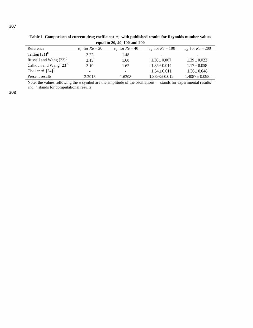
Table 1 Comparison of current drag coefficient dc with published results for Reynolds number values

equal to 20, 40, 100 and 200 Reference dc for Re = 20 dc for Re = 40 dc for Re = 100 dc for Re = 200

Tritton [21]E 2.22 1.48 - - Russell and Wang [22]C 2.13 1.60 1.38 0.007 1.29 0.022Calhoun and Wang [23]C 2.19 1.62 1.35 0.014 1.17 0.058Choi et al. [24]C - - 1.34 0.011 1.36 0.048Present results 2.2013 1.6208 1.3898 0.012 1.4087 0.098Note: the values following the ± symbol are the amplitude of the oscillations, E stands for experimental results and C stands for computational results

   308 

309 

Table 2 Summary of results for St = 0.4, Re = 1100

Airfoil type 0.1(2.0)a hh f 0.3(0.66666)a hh f

tc Pc

lc ˆlc tc Pc

lc ˆlc

NACA 0012 0.8515 7.5748 0.1124 0.0093 28.17 0.8292 5.3332 0.1554 0.0144 11.30 NACA 2212 0.9326 7.6910 0.1212 0.0283 27.02 0.8244 5.3221 0.1549 0.2279 11.08 NACA 2412 0.9329 7.7209 0.1208 0.1120 27.12 0.8486 5.3313 0.1591 0.1074 10.48 NACA 4412 0.9080 7.6433 0.1188 0.4465 27.44 0.8035 5.2321 0.1535 0.1584 10.75 NACA 2612 0.9286 7.7304 0.1201 0.2475 28.54 0.8340 5.3293 0.1565 0.3194 11.41 NACA 4612 0.8920 7.6356 0.1168 0.7074 28.81 0.8067 5.2851 0.1526 0.3963 11.54 NACA 6612 0.8664 7.5440 0.1148 1.1194 28.25 0.7627 5.1025 0.1494 0.4675 12.70 Selig S1223 0.7944 7.2373 0.1097 1.4181 29.58 0.4284 4.4070 0.0972 0.2658 11.58

310 

311 

Table 3 Summary of results for St = 0.3, Re = 1100

Airfoil type 0.1(1.5)a hh f 0.3(0.5)a hh f

tc Pc lc ˆlc tc Pc

lc ˆlc

NACA 0012 0.3928 2.8441 0.1381 0.0123 15.36 0.2487 2.0851 0.1193 0.0069 6.37 NACA 2212 0.4039 2.8998 0.1393 0.0391 15.58 0.2391 2.1146 0.1130 0.1701 6.43 NACA 2412 0.4048 2.9115 0.1390 0.2000 15.59 0.2388 2.1114 0.1131 0.1962 6.48 NACA 4412 0.3911 2.9078 0.1345 0.4871 15.81 0.2306 2.0715 0.1113 0.3845 6.59 NACA 2612 0.4018 2.9051 0.1383 0.3018 15.66 0.2382 2.1139 0.1126 0.2371 6.56 NACA 4612 0.3815 2.8886 0.1321 0.6580 15.93 0.2244 2.0692 0.1084 0.4738 6.74 NACA 6612 0.3483 2.8655 0.1215 0.9983 16.19 0.1997 2.0099 0.0993 0.6799 6.87 Selig S1223 0.3562 2.9019 0.1227 1.0351 16.61 0.1602 1.7992 0.0890 0.6366 6.61

312 

313 

Table 4 Summary of results for St = 0.2, Re = 1100

Airfoil type 0.1(1.0)a hh f 0.3(0.33333)a hh f

tc Pc

lc ˆlc tc Pc

lc ˆlc

NACA 0012 0.0608 0.8299 0.0733 0.0091 6.35 0.0386 0.6201 0.0623 0.0081 2.27 NACA 2212 0.0717 0.8002 0.0896 0.1065 6.52 0.0480 0.6757 0.0710 0.0198 2.45 NACA 2412 0.0723 0.7983 0.0906 0.1207 6.52 0.0462 0.6457 0.0715 0.0656 2.43 NACA 4412 0.0580 0.8023 0.0723 0.3546 6.75 0.0381 0.6877 0.0554 0.1883 2.50 NACA 2612 0.0723 0.7985 0.0906 0.1624 6.56 0.0495 0.6586 0.0752 0.0891 2.44 NACA 4612 0.0575 0.7904 0.0727 0.3820 6.83 0.0361 0.6607 0.0547 0.1708 2.53 NACA 6612 0.0332 0.7796 0.0425 0.5947 7.09 0.0106 0.6188 0.0172 0.2046 2.57 Selig S1223 0.0004 0.8863 0.0004 0.9698 7.37 -0.049 0.6297 - 0.2196 2.42 Note: for negative thrust coefficients, the propulsive efficiency is not shown

 314 

   315 

 316 

Table 5 t lc c product for each heaving configuration

Airfoil type for 0.2t lc c St for 0.3t lc c St for 0.4t lc c St

0.1ah 0.3ah 0.1ah 0.3ah 0.1ah 0.3ah

NACA 0012 0.0005 0.0003 0.0048 0.0017 0.0079 0.0119 NACA 2212 0.0076 0.0009 0.0157 0.0406 0.0263 0.1878 NACA 2412 0.0087 0.0030 0.0809 0.0468 0.1044 0.0911 NACA 4412 0.0205 0.0071 0.1905 0.0886 0.4054 0.1272 NACA 2612 0.0117 0.0044 0.1212 0.0564 0.2298 0.2663 NACA 4612 0.0219 0.0061 0.2510 0.1063 0.6310 0.3196 NACA 6612 0.0197 0.0021 0.3477 0.1357 0.9698 0.3565 Selig S1223 0.0003 -0.0107 0.3687 0.1019 1.1265 0.1138

 317 

   318 

List of figure captions 319 

320 

Fig. 2 Simple overlapping grid system in physical space , for the sample case of the flow past a cylinder 321 

 322 

Fig. 2 Comparison of thrust coefficient tc and propulsive efficiency variation with the 323 

Strouhal number St (Re = 40000) 324 

 325 

Fig. 3 Overlapping grid system layout for the heaving airfoil case 326 

 327 

Fig. 4 NACA 0012 and NACA 6612 lift coefficient and thrust coefficient (equal to negative drag) comparison. Top 328 

figure: instantaneous lift coefficient time evolution. Bottom figure: instantaneous drag coefficient time evolution. Heaving 329 

parameters: Re = 1100, St = 0.3, 0.3ah = 330 

 331 

Fig. 5 Comparison of the vorticity field for two different airfoils. Left column: NACA 0012 airfoil. Right column: Selig 332 

S1223 airfoil. Heaving parameters: Re = 1100, St = 0.4, 0.3ah = . The sequence is shown for four instants during the 333 

upstroke motion, where: A) t = 9.0, B) t = 9.25, C) t = 9.50, D) t = 9.75 334 

335