Page 1
EFFECT OF CYCLIC SWELL-SHRINK ON SWELL PERCENTAGE OF AN EXPANSIVE CLAY STABILIZED BY CLASS C FLY ASH
A THESIS SUBMITTED TO THE GRADUATE SCHOOL OF NATURAL AND APPLIED SCIENCES
OF MIDDLE EAST TECHNICAL UNIVERSITY
BY
MEHMET AS
IN PARTIAL FULFILLMENT OF THE REQUIREMENTS FOR
THE DEGREE OF MASTER OF SCIENCE IN
CIVIL ENGINEERING
JANUARY 2012
Page 2
Approval of the thesis:
EFFECT OF CYCLIC SWELL-SHRINK ON SWELL PERCENTAGE OF AN EXPANSIVE CLAY STABILIZED BY CLASS C FLY ASH
submitted by MEHMET AS in partial fulfillment of the requirements for the degree of Master of Science in Civil Engineering Department, Middle East Technical University by, Prof. Dr. Canan Özgen ____________ Dean, Graduate School of Natural and Applied Sciences Prof. Dr. Güney Özcebe ____________ Head of Department, Civil Engineering Prof. Dr. Erdal Çokça ____________ Supervisor, Civil Engineering Dept., METU
Examining Committee Members:
Prof. Dr. M. Yener Özkan ____________________ Civil Engineering Dept., METU
Prof. Dr. Erdal Çokça ____________________ Civil Engineering Dept., METU
Assist. Prof. Dr. Nejan Huvaj Sarıhan ____________________ Civil Engineering Dept., METU
Dr. Onur Pekcan ____________________ Civil Engineering Dept., METU
Mustafa Toker, M.Sc. ____________________ Toker Drilling and Cons. Co.
Date: 27.01.2012
Page 3
iii
I hereby declare that all information in this document has been obtained and presented in accordance with academic rules and ethical conduct. I also declare that, as required by these rules and conduct, I have fully cited and referenced all material and results that are not original to this work.
Name, Last Name : MEHMET AS
Signature :
Page 4
iv
ABSTRACT
EFFECT OF CYCLIC SWELL – SHRINK ON SWELL PERCENTAGE
OF AN EXPANSIVE CLAY STABILIZED BY CLASS C FLY ASH
As, Mehmet
M.Sc., Department of Civil Engineering
Supervisor: Prof. Dr. Erdal Çokça
January 2012, 115 pages
Expansive soils are a worldwide problem especially in the regions where
climate is arid or semi arid. These soils swell when they are exposed to water
and shrink when they dry. Cyclic swelling and shrinkage of clays and
associated movements of foundations may result in cracking of structures.
Several methods are used to decrease or prevent the swelling potential of
such soils like prewetting, surcharge loading, chemical stabilization etc.
Among these, one of the most widely used method is using chemical
admixtures (chemical stabilization). Cyclic wetting and drying affects the
swell – shrink behaviour of expansive soils. In this research, the effect of
cyclic swell – shrink on swell percentage of a chemically stabilized expansive
soil is investigated. Class C Fly Ash is used as an additive for stabilization of
an expansive soil that is prepared in the laboratory environment by mixing
kaolinite and bentonite. Fly ash was added to expansive soil with a
predetermined percentage changing between 0 to 20 percent. Hydrated lime
with percentages changing between 0 to 5 percent and sand with 5 percent
were also used instead of fly ash for comparison. Firstly, consistency limits,
grain size distributions and swell percentages of mixtures were determined.
Then to see the effect of cyclic swell – shrink on the swelling behavior of the
mixtures, swell – shrink cycles applied to samples and swell percentages were
Page 5
v
determined. Swell percentage decreased as the proportion of the fly ash
increased. Cyclic swell-shrink affected the swell percentage of fly ash
stabilized samples positively.
Keywords: Cyclic Swell-Shrink, Expansive Soil, Class C Fly Ash, Swell
Percantage, Drying- Wetting
Page 6
vi
ÖZ
DÖNGÜSEL 9İ9ME VE BÜZÜ9MENİN C SINIFI UÇUCU KÜL İLE
STABİLİZE EDİLEN 9İ9EN ZEMİNİN, 9İ9ME YÜZDESİ ÜZERİNDEKİ ETKİSİ
As, Mehmet
Yüksek Lisans, İnşaat Mühendisliği Bölümü
Tez Yöneticisi: Prof. Dr. Erdal Çokça
Ocak 2012, 115 sayfa
Lişen zeminler, özellikle iklimin kurak veya yarı kurak olduğu bölgelerde olmak
üzere bütün dünyada problem oluşturmaktadır. Bu zeminler suya maruz
bırakıldıklarında şişmekte, kuruduklarında ise büzüşmektedirler. Döngüsel
şişme ve büzüşme ve yapı temellerinde meydana getirdikleri hareketler
yapılarda çatlaklara neden olmaktadır. Bu tarz zeminlerin şişme potansiyelini
düşürmek veya ortadan kaldırmak için ön ıslatma, ilave yükleme ve kimyasal
stabilizasyon gibi bir çok metot kullanılmaktadır. Bu metotlar arasında en
yaygın olanlardan biri kimyasal katkı kullanmaktır (kimyasal stabilizasyon).
Döngüsel ıslanma ve kuruma şişen zeminlerin şişme - büzüşme davranışlarını
etkilemektedir. Bu araştırmada döngüsel şişme - büzüşmenin kimyasal katkı
yardımıyla stabilizasyonu sağlanan şişen zeminlerin şişme yüzdeleri
üzerindeki etkisi incelenmiştir. Laboratuar ortamında kaolin ve bentonit
karıştırılarak elde edilen şişen zeminin stabilizasyonu için katkı maddesi olarak
C Sınıfı Uçucu Kül kullanılmıştır. Uçucu kül şişen zemine önceden belirlenen,
%0 ile %20 arasında değişen, oranlarda eklenmiştir. Ayrıca deneylerde
karşılaştırma amacıyla, uçucu kül yerine %1 ile %5 oranında değişen sönmüş
kireç ve %5 oranında kum kullanılmıştır. Öncelikle karışımların kıvam limitleri,
dane boyu dağılımları ve şişme yüzdeleri belirlenmiştir. Daha sonra döngüsel
Page 7
vii
şişme - büzüşmenin numunelere etkisini görmek için numuneler şişme –
büzüşmeye maruz bırakılmış ve şişme yüzdeleri belirlenmiştir. Numunelerin
şişme yüzdeleri uçucu kül oranı arttıkça azalma göstermiştir. Döngüsel şişme-
büzüşmenin ise uçucu kül ile stabilize edilen numunelerin şişme yüzdelerini
pozitif olarak etkilediği gözlenmiştir.
Anahtar Kelimeler: Döngüsel Lişme - Büzüşme, Lişen Zeminler, C Sınıfı
Uçucu Kül, Lişme Yüzdesi, Kuruma - Islanma
Page 9
ix
ACKNOWLEDGEMENTS
I would like to express sincere appreciation to my supervisor, Prof. Dr. Erdal
Çokça for his guidance, continuous understanding, invaluable patience and
support throughout this research.
I also wish to express my special thanks to Dr. Kartal Toker for his valuable
advices throughout the laboratory works.
Special thanks go to the staff of Toker Drilling and Construction Co., especially
to Mustafa Toker for their great encouragements during my studies.
My thankfulness goes to geology engineer Mr. Ulaş Nacar and technician
Mr. Kamber Bilgen for their support and friendly approach throughout the
laboratory works.
I would like to acknowledge my friends Melih Bozkurt, Nilsu Kıstak, Güliz Ünlü,
Ertaç Tuç, Mustafa Bilal and Erdem İspir for their helpful suggestions and
encouragements during this study.
Finally, I express my sincere thanks to my aunt Sibel Ören, to my sister Merve
As and to my mother Ayşe As for their endless supports throughout my life.
Page 10
x
TABLE OF CONTENTS
ABSTRACT .................................................................................................... iv
ÖZ ................................................................................................................ vi
ACKNOWLEDGEMENTS ............................................................................... ix
TABLE OF CONTENTS................................................................................... x
LIST OF TABLES .......................................................................................... xii
LIST OF FIGURES ....................................................................................... xiv
LIST OF ABBREVIATIONS .......................................................................... xiv
CHAPTERS
1. INTRODUCTION ...................................................................................... 1
1.1 General ............................................................................................. 1
1.2 Aim of the Study ................................................................................ 2
1.3 Scope of the Study ............................................................................ 2
2. LITERATURE REVIEW ............................................................................ 4
2.1 Expansive Soils ................................................................................. 4
2.1.1 Clay Mineralogy.......................................................................... 4
2.1.2 Factors Influencing Swelling ..................................................... 11
2.2 Soil Stabilization .............................................................................. 15
2.2.1 Chemical Stabilization .............................................................. 15
2.2.2 Lime Stabilization ..................................................................... 15
2.2.3 Fly Ash Stabilization ................................................................. 17
3. FLY ASH ................................................................................................ 18
3.1 General ........................................................................................... 18
3.2 Factors that influence Fly Ash Properties ........................................ 20
3.2.1 Coal Source ............................................................................. 20
3.2.2 Boiler and Emission Control Design ......................................... 20
3.3 Classification of Fly Ashes ............................................................... 21
3.4 Soma Thermal Power Plant ............................................................. 21
3.5 Utilization of Fly Ash ........................................................................ 23
Page 11
xi
4. PREVIOUS STUDIES ON CYCLIC SWELL-SHRINK BEHAVIOUR OF SOILS ............................................................................................................ 26
4.1 General ........................................................................................... 26
4.2 Studies on Nonstabilized Soils ........................................................ 26
4.3 Studies on Stabilized Soils .............................................................. 31
5. EXPERIMENTAL WORKS ..................................................................... 40
5.1 Purpose ........................................................................................... 40
5.2 Materials.......................................................................................... 40
5.3 Preparation and Properties of Test Samples ................................... 43
5.4 Properties of Samples ..................................................................... 46
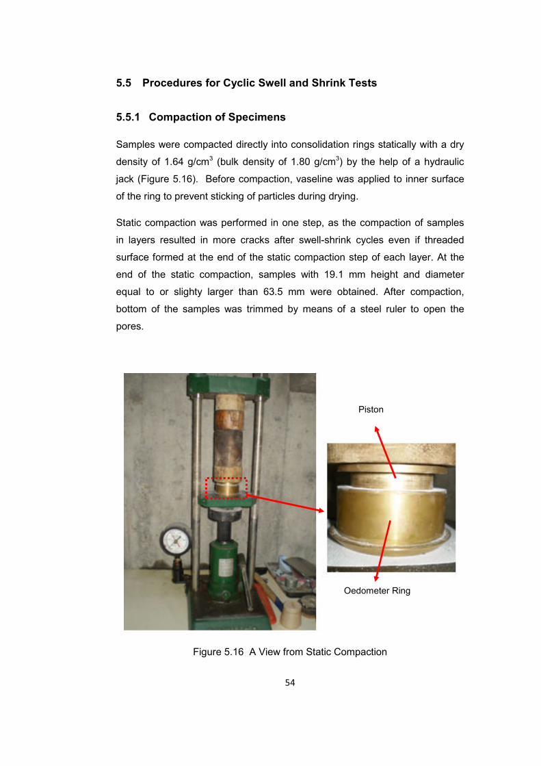
5.5 Procedures for Cyclic Swell and Shrink Tests ................................. 54
5.5.1 Compaction of Specimens ........................................................ 54
5.5.2 Cyclic Swell – Shrink Tests ...................................................... 55
5.5.3 Test Results ............................................................................. 59
5.6. SEM – EDX Analysis ....................................................................... 72
6. DISCUSSION ON TEST RESULTS ....................................................... 79
6.1 Effect of Additives on Grain Size Distribution ................................... 79
6.2 Effect of Additives on Specific Gravity ............................................. 80
6.3 Effect of Additives on Liquid Limit .................................................... 81
6.4 Effect of Additives on Plastic Limit ................................................... 82
6.5 Effect of Additives on Plasticity Index .............................................. 82
6.6 Effect of Additives on Shrinkage Limit ............................................. 82
6.7 Effect of Additives on Linear Shrinkage ........................................... 83
6.8 Effect of Additives on Shrinkage Index ............................................ 83
6.9 Effect of Additives on Activity ........................................................... 84
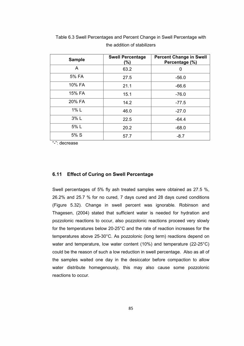
6.10 Effect of Additives on Swell Percentage .......................................... 84
6.11 Effect of Curing on Swell Percentage .............................................. 85
6.12 Effect of Cyclic Swell-Shrink on Swell Percentages of Samples ...... 86
6.13 Discussions on SEM-EDX Analysis ................................................. 91
7. CONCLUSIONS ..................................................................................... 93
REFERENCES .............................................................................................. 97
APPENDICES
A- CHEMICAL ANALYSIS REPORT OF SOMA FLY ASH .......................... 103
B- SWELL VERSUS TIME GRAPHS .......................................................... 104
Page 12
xii
LIST OF TABLES
TABLES
Table 2.1 Soil Properties that influence shrink-swell potential
(Nelson and Miller, 1992)............................................................................... 12
Table 2.2 Environmental Conditions that influence shrink-swell potential
(Nelson and Miller, 1992)............................................................................... 13
Table 2.3 Stress Conditions that influence shrink-swell potential
(Nelson and Miller, 1992)............................................................................... 14
Table 3.1 Utilization of Fly Ash by 2009 in USA (ACAA, 2011) ...................... 25
Table 4.1 Swell-Shrink Procedures applied on nonstabilized expansive soils in
previous studies by different researchers ...................................................... 30
Table 4.1 Swell-Shrink Procedures applied on nonstabilized expansive soils in
previous studies by different researchers (continued). ................................... 31
Table 4.2 Properties of the materials used in Güney et al, (2007) studies. .... 33
Table 4.3 Swell-Shrink Procedures applied on stabilized expansive soils in
previous studies by different researchers ...................................................... 38
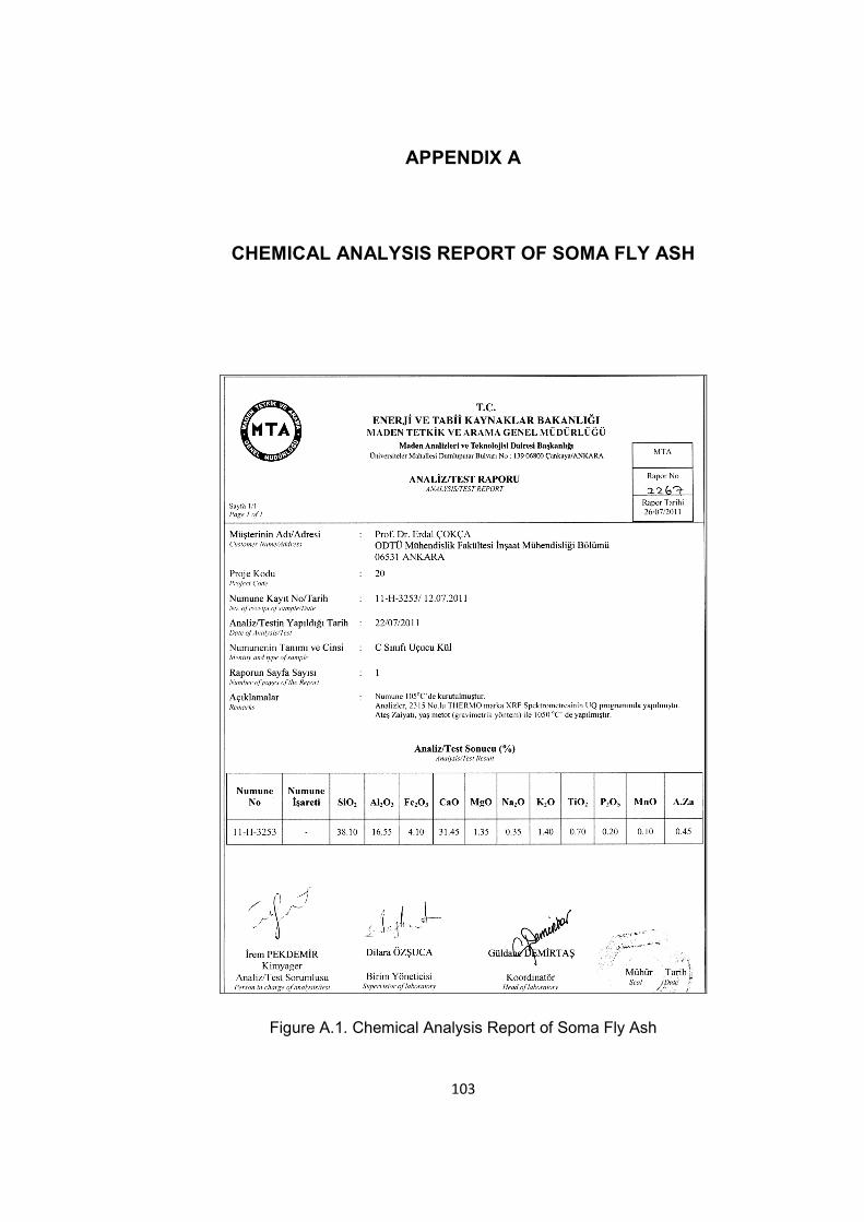
Table 5.1 Chemical Composition of Fly Ash and Lime ................................... 41
Table 5.2 Composition of Prepared Specimens ............................................. 44
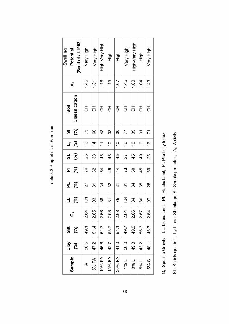
Table 5.3 Properties of Samples .................................................................... 53
Table 5.4 Samples chosen for SEM Analysis ................................................ 72
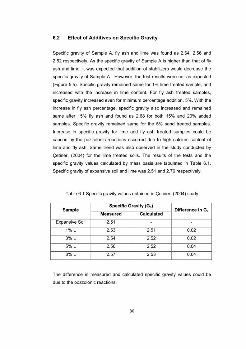
Table 6.1 Specific gravity values obtained in Çetiner, (2004) study ............... 80
Table 6.2 Percent Changes in Specific Gravity (Gs), Liquid Limit (LL), Plastic
Limit (PL), Plasticity Index (PI), Shrinkage Limit (SL), Linear Shrinkage (Ls),
Shrinkage Index (SI) and Activity (Ac) ............................................................ 81
Table 6.3 Swell Percentages and Percent Change in Swell Percentage with
the addition of stabilizers ............................................................................... 85
Page 13
xiii
Table 6.4. Axial swell percentages (∆Hi/Hid) of samples ................................ 86
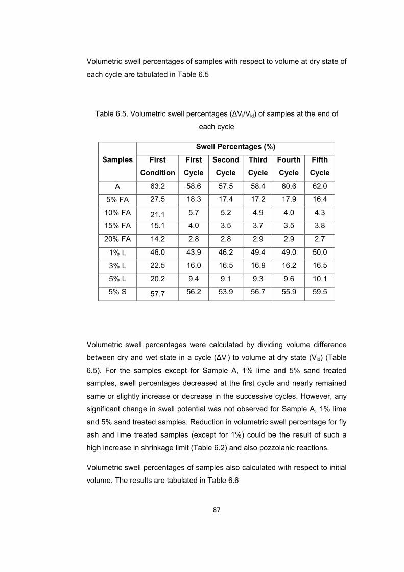
Table 6.5. Volumetric swell percentages (∆Vi/Vid) of samples at the end of
each cycle ..................................................................................................... 87
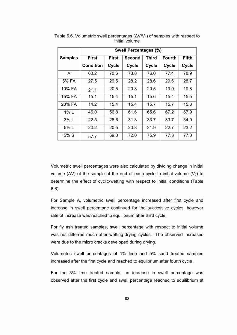
Table 6.6. Volumetric swell percentages (∆V/V0) of samples with respect to
initial volume .................................................................................................. 88
Table 6.7. Swell percentages for 5% fly ash samples with no cure, 7 days
cured and 28 days cured ............................................................................... 90
Table 6.8. Curing conditions and unconfined compressive strength (qu) values
in Beeghly, (2003) study. ............................................................................... 91
Page 14
xiv
LIST OF FIGURES
FIGURES Figure 2.1 Basic Unit of Clay Minerals (Craig, 1997) ....................................... 5
Figure 2.2 Synthesis pattern of Clay Minerals (modified from Mitchell, 2005) .. 6
Figure 2.3 Structure of Kaolinite (USGS, 2001) ............................................... 7
Figure 2.4 Scanning Electron Micrograph of Kaolinite (Murray, 2007) ............. 7
Figure 2.5 Structure of Illite (USGS, 2001) ...................................................... 8
Figure2.6 Scanning Electron Micrograph of Illite(source:http://webmineral.
com /specimens/picshow.php?id=1284&target=Illite) ...................................... 9
Figure 2.7 Structure of Montmorillonite (USGS, 2001) ................................... 10
Figure 2.8 Scanning Electron Micrograph of Sodium Montmorillonite (Murray,
2007) ............................................................................................................. 10
Figure 3.1 Coal Ash Pollution Chain (Greenpeace,2010)............................... 19
Figure 3.2 Ash Disposal Site of Soma Thermal Power Plant
(Baba and Kaya, 2004) .................................................................................. 22
Figure 3.3 Scanning Electron Micrograph of Soma Fly Ash
(Çelik, 2004) .................................................................................................. 23
Figure 3.4 Fly Ash production and utilization statistics for USA (adapted from
American Coal Ash Association, 2011) .......................................................... 24
Figure 3.5 Fly Ash production and utilization comparison for USA (adapted
from American Coal Ash Association, 2011) .................................................. 24
Figure 4.1 Total pressure cells data for the Power House linings of Masjed-
Soleiman Hydroelectric Power Plant Project (Doostmohammadi, 2009) ........ 28
Figure 4.2 Effect of full swell-full shrink and full swell-partial shrink on swell
potential of an expansive soil (Tawfiq & Nalbantoğlu, 2009) .......................... 29
Page 15
xv
Figure 4.3 Effect of wetting-drying cycles on clay content of lime treated soils
(Rao, 2011) ................................................................................................... 32
Figure 4.4 Effect of wetting-drying cycles on plastic limit of lime treated soils
(Rao, 2011) ................................................................................................... 32
Figure 4.5 Change of Swell Percent for Soil A and lime treated Soil A
(Güney et al, 2007) ........................................................................................ 34
Figure 4.6 Change of Swell Percent for Soil C and lime treated Soil C (Güney
et al, 2007) .................................................................................................... 34
Figure 4.7 Experimental set up used in Rao A.& Rao M.,( 2008) studies ...... 35
Figure 4.8 Cyclic swell-shrink behavior of samples containg 20% bentonite
treated with lime (Akcanca & Aytekin, 2011) .................................................. 36
Figure 4.9 Cyclic swell-shrink behavior of expansive soil stabilized with silica
fume (Kalkan, 2011) ...................................................................................... 37
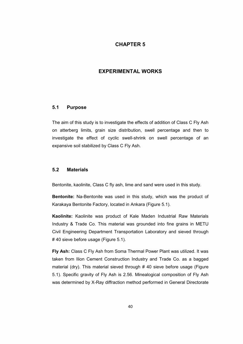
Figure 5.1. Views from Materials (1-kaolinite, 2-bentonite, 3-fly ash,
4-lime) ........................................................................................................ 41
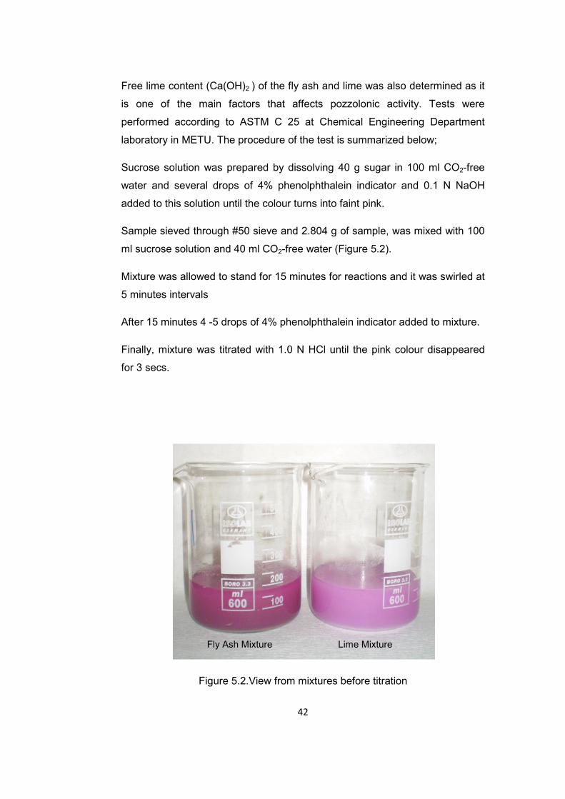
Figure 5.2.View from mixtures before titration ................................................ 42
Figure 5.3. Preparation of Samples ............................................................... 45
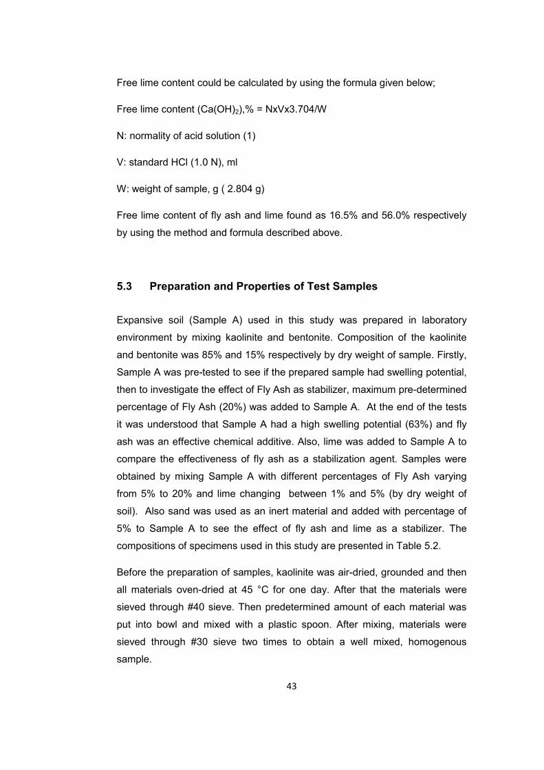
Figure 5.4. Crystals formed in fly ash during the hydrometer test .................. 46
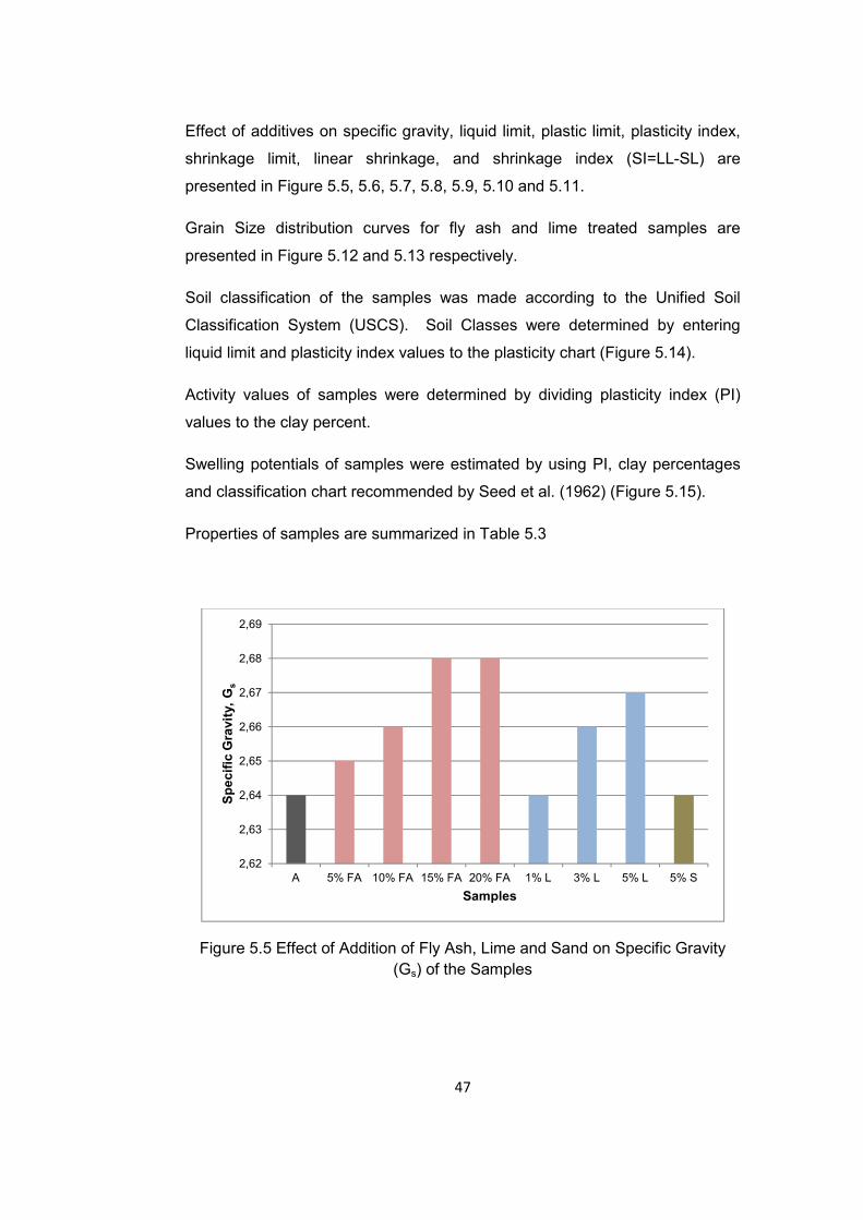
Figure 5.5 Effect of Addition of Fly Ash, Lime and Sand on Specific Gravity
(Gs) of the Samples ....................................................................................... 47
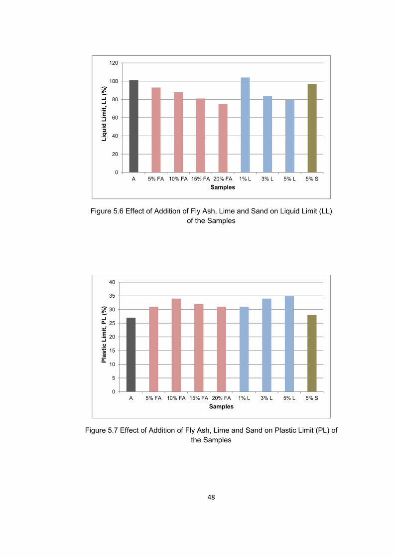
Figure 5.6 Effect of Addition of Fly Ash, Lime and Sand on Liquid Limit (LL) of
the Samples.................................................................................................... 48
Figure 5.7 Effect of Addition of Fly Ash, Lime and Sand on Plastic Limit (PL)
of the Samples .............................................................................................. 48
Figure 5.8 Effect of Addition of Fly Ash, Lime and Sand on Plasticity Index (PI)
of the Samples .............................................................................................. 49
Figure 5.9 Effect of Addition of Fly Ash, Lime and Sand on Shrinkage Limit
(SL) of the Samples ....................................................................................... 49
Figure 5.10 Effect of Addition of Fly Ash, Lime and Sand on Linear Shrinkage
(Ls) of the Samples ........................................................................................ 50
Page 16
xvi
Figure 5.11 Effect of Addition of Fly Ash, Lime and Sand on Shrinkage Index
(SI) of the Samples ........................................................................................ 50
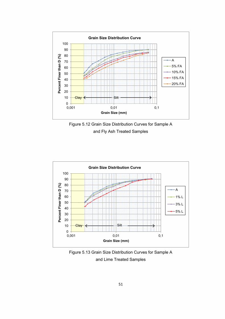
Figure 5.12 Grain Size Distribution Curves for Sample A and Fly Ash Treated
Samples ........................................................................................................ 51
Figure 5.13 Grain Size Distribution Curves for Sample A and Lime Treated
Samples ........................................................................................................ 51
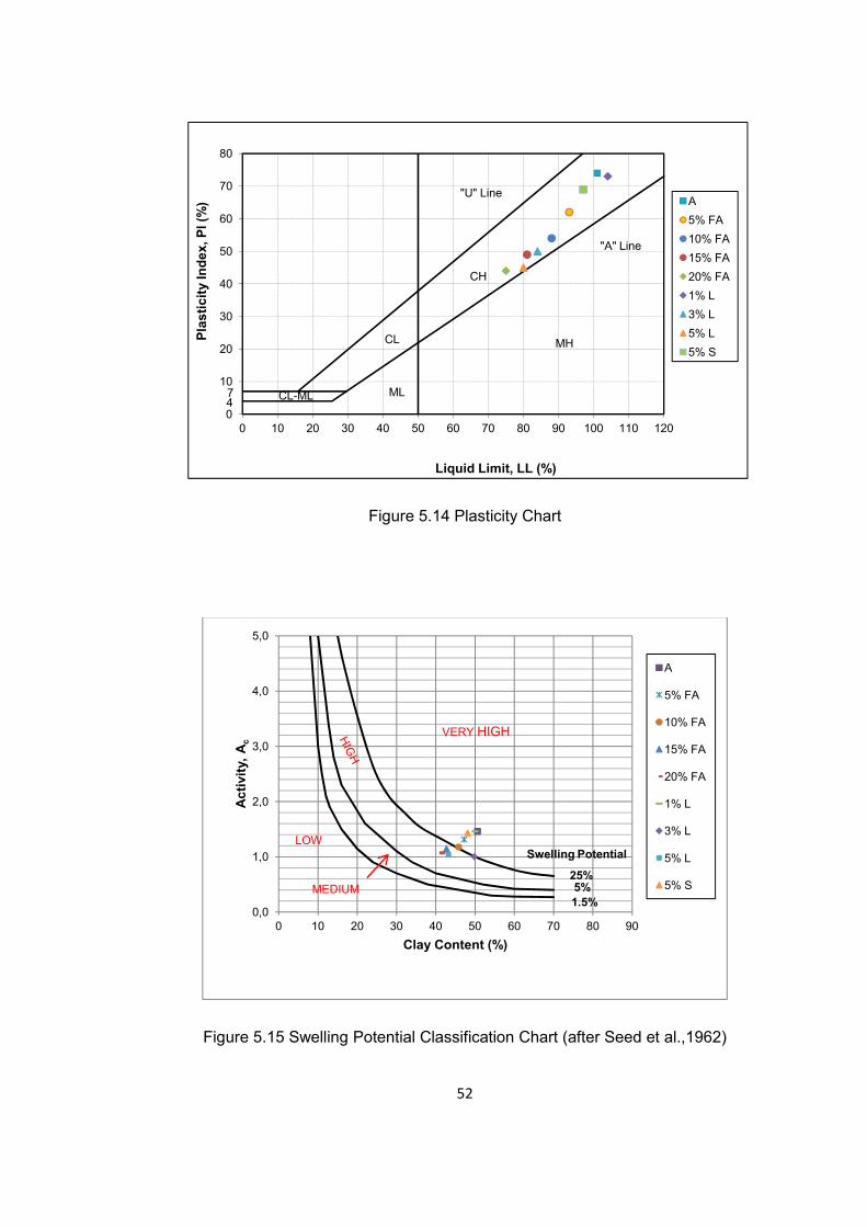
Figure 5.14 Plasticity Chart ............................................................................ 52
Figure 5.15 Swelling Potential Classification Chart (after Seed et al.,1962) ... 52
Figure 5.16 View from Static Compaction ...................................................... 54
Figure 5.17 Free Swell Test Setup Drawing (İpek, 1998) ............................... 55
Figure 5.18 View from Oedometers during testing ......................................... 56
Figure 5.19 Measuring height with digital caliper ........................................... 57
Figure 5.20 Measuring volume with mercury ................................................. 57
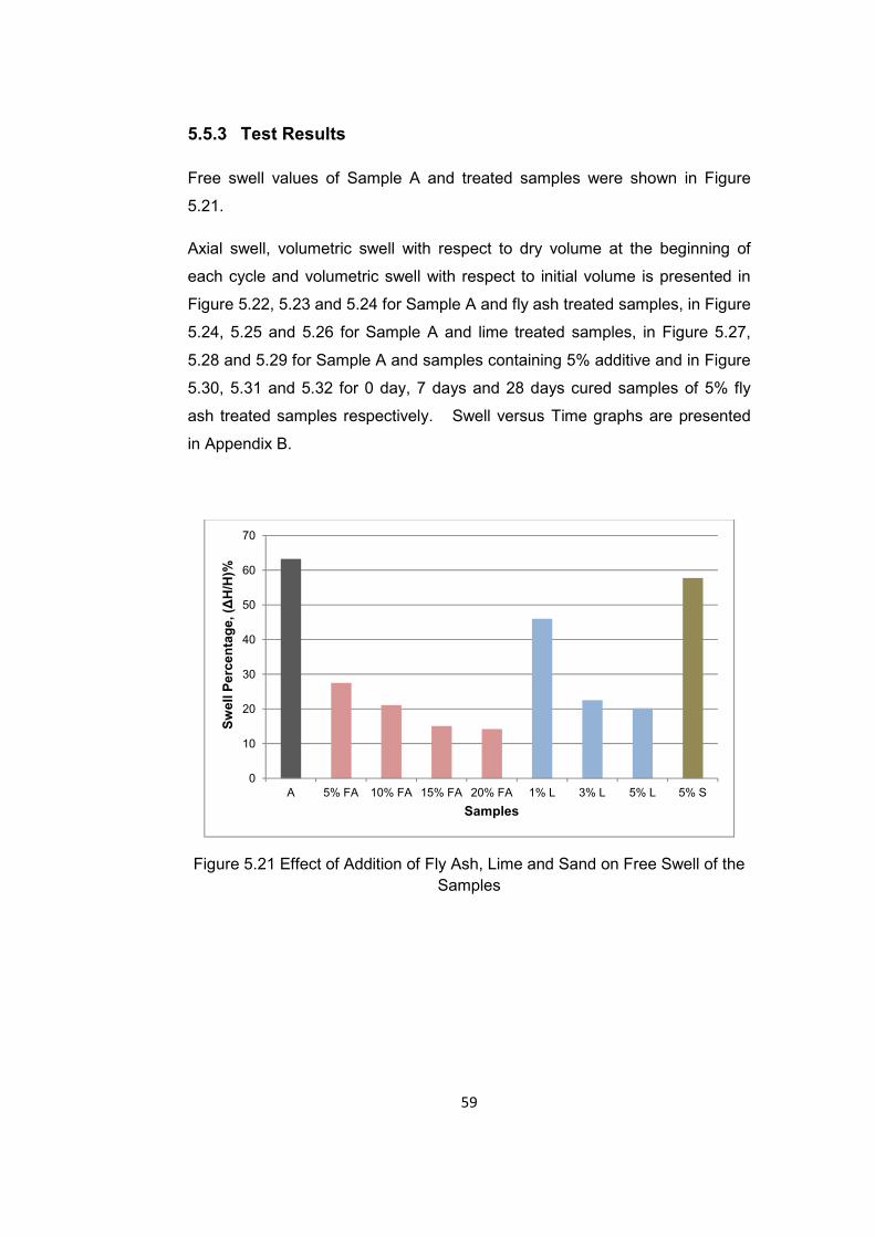
Figure 5.21 Effect of Addition of Fly Ash, Lime and Sand on Free Swell of the
Samples ........................................................................................................ 58
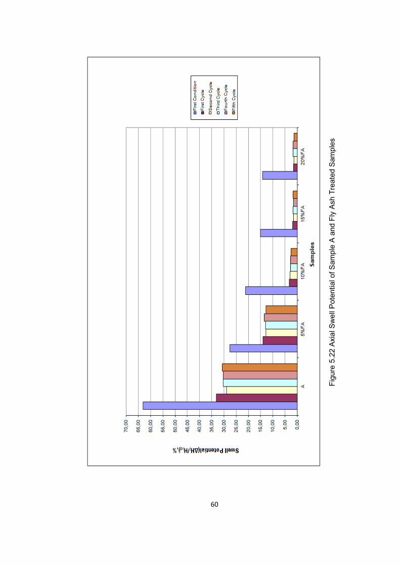
Figure 5.22 Axial Swell Potential of Sample A and Fly Ash Treated
Samples ........................................................................................................ 60
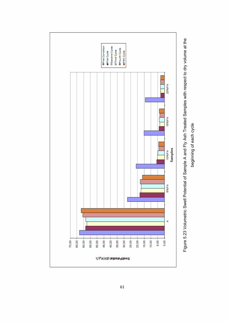
Figure 5.23 Volumetric Swell Potential of Sample A and Fly Ash Treated
Samples with respect to dry volume at the beginning of each cycle ............... 61
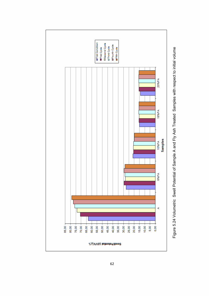
Figure 5.24 Volumetric Swell Potential of Sample A and Fly Ash Treated
Samples with respect to initial volume ........................................................... 62
Figure 5.25 Axial Swell Potential of Sample A and Lime Treated
Samples ........................................................................................................ 63
Figure 5.26 Volumetric Swell Potential of Sample A and Lime Treated
Samples with respect to dry volume at the beginning of each cycle ............... 64
Figure 5.27 Volumetric Swell Potential of Sample A and Lime Treated
Samples with respect to initial volume ........................................................... 65
Figure 5.28 Axial Swell Potential of Sample A and Samples containing 5%
Additives ........................................................................................................ 66
Page 17
xvii
Figure 5.29 Volumetric Swell Potential of Sample A and Samples containing
5% Additives with respect to dry volume at the beginning of each
cycle .............................................................................................................. 67
Figure 5.30 Volumetric Swell Potential of Sample A and Samples containing
5% Additives with respect to initial volume .................................................... 68
Figure 5.31 Axial Swell Potential of 5% fly ash added Samples with and
without curing ................................................................................................ 69
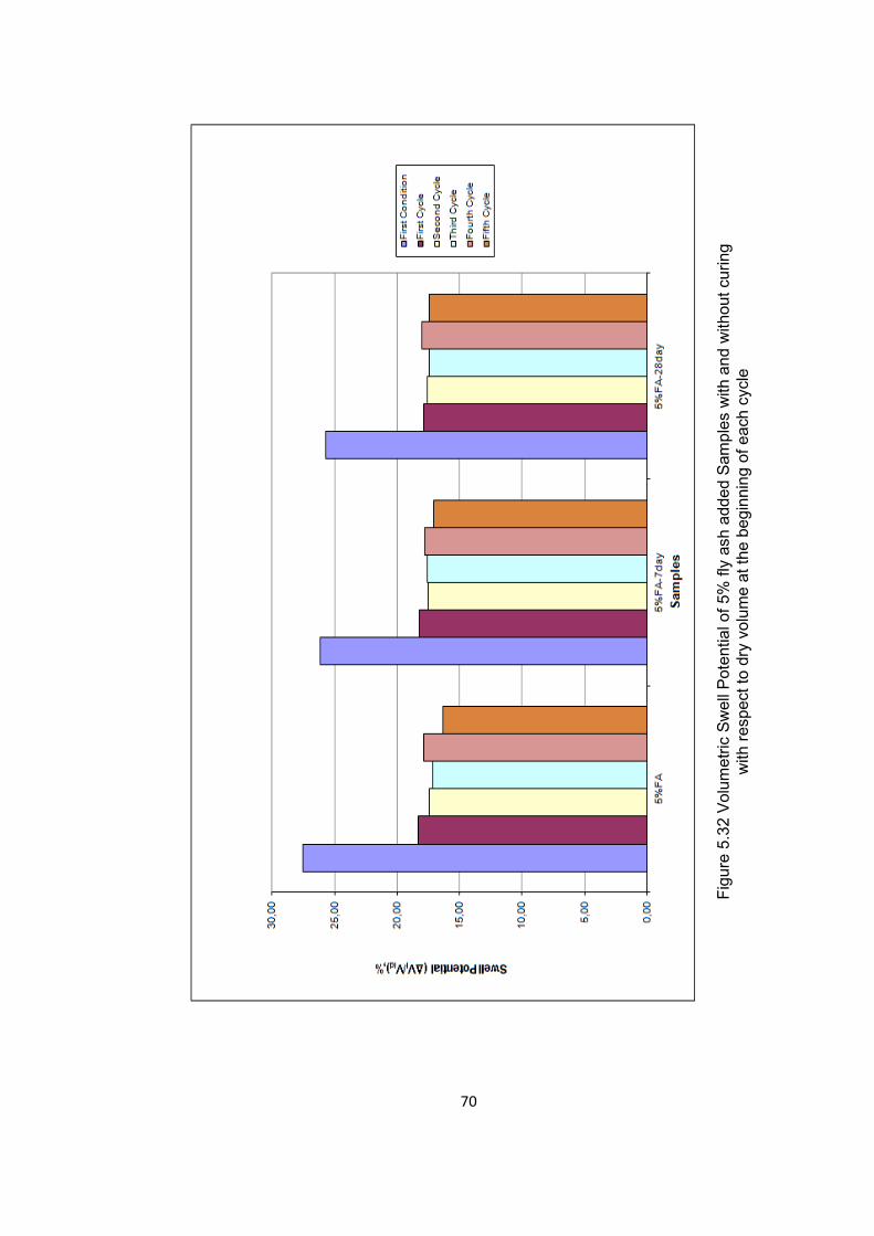
Figure 5.32 Volumetric Swell Potential of of 5% fly ash added Samples with
and without curing with respect to dry volume at the beginning of each
cycle .............................................................................................................. 70
Figure 5.33 Volumetric Swell Potential of 5% fly ash added Samples with and
without curing with respect to initial volume ................................................... 71
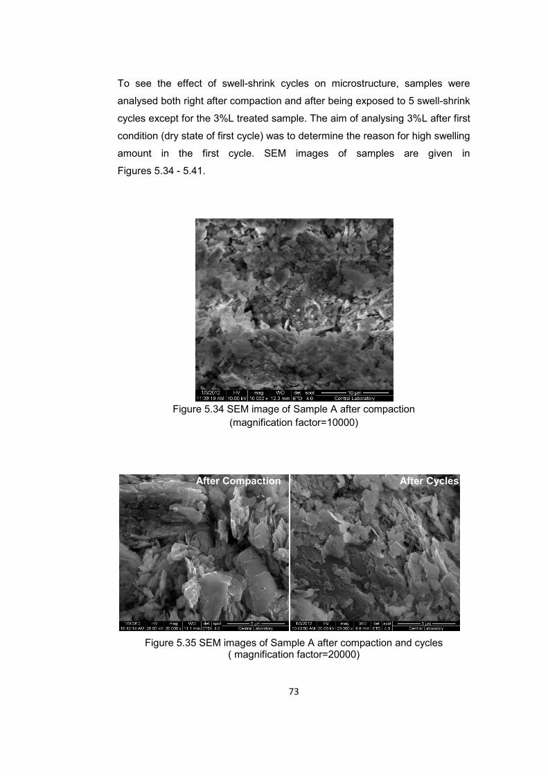
Figuren5.34 SEM image of Sample A after compaction (magnification
factor=10000) ................................................................................................ 73
Figure 5.35 SEM images of Sample A after compaction and cycles
(magnification factor=20000) ......................................................................... 71
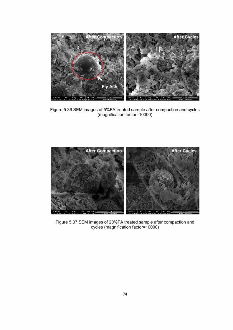
Figure 5.36 SEM images of 5%FA treated sample after compaction and cycles
(magnification factor=10000) ......................................................................... 73
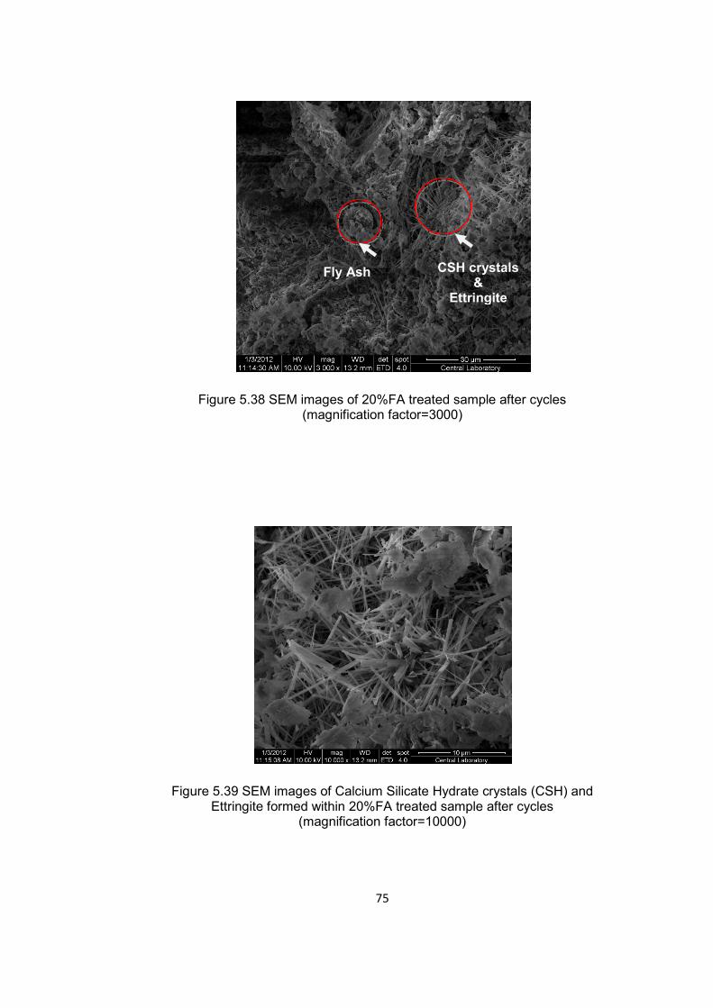
Figure 5.37 SEM images of 20%FA treated sample after compaction and
cycles (magnification factor=10000) .............................................................. 74
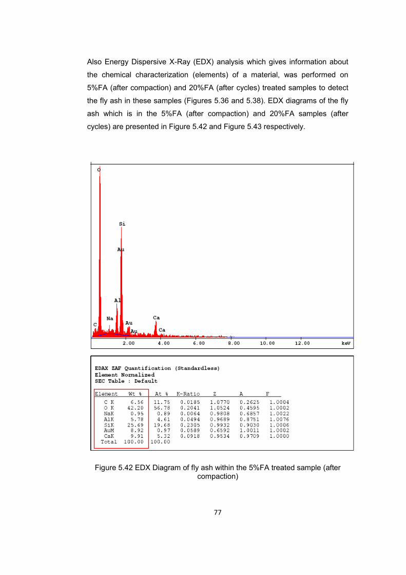
Figure 5.38 SEM images of 20%FA treated sample after cycles (magnification
factor=3000) .................................................................................................. 75
Figure 5.39 SEM images of Calcium Silicate Hydrate crystals (CSH) and
Ettringite formed within 20%FA treated sample after cycles (magnification
factor=10000) ................................................................................................ 75
Figure 5.40 SEM images of 3%L treated sample after compaction and first
condition (at dry state of first cycle) (magnification factor=20000) .................. 76
Figure 5.41 SEM images of 5%L treated sample after compaction and cycles
(magnification factor=10000) ......................................................................... 76
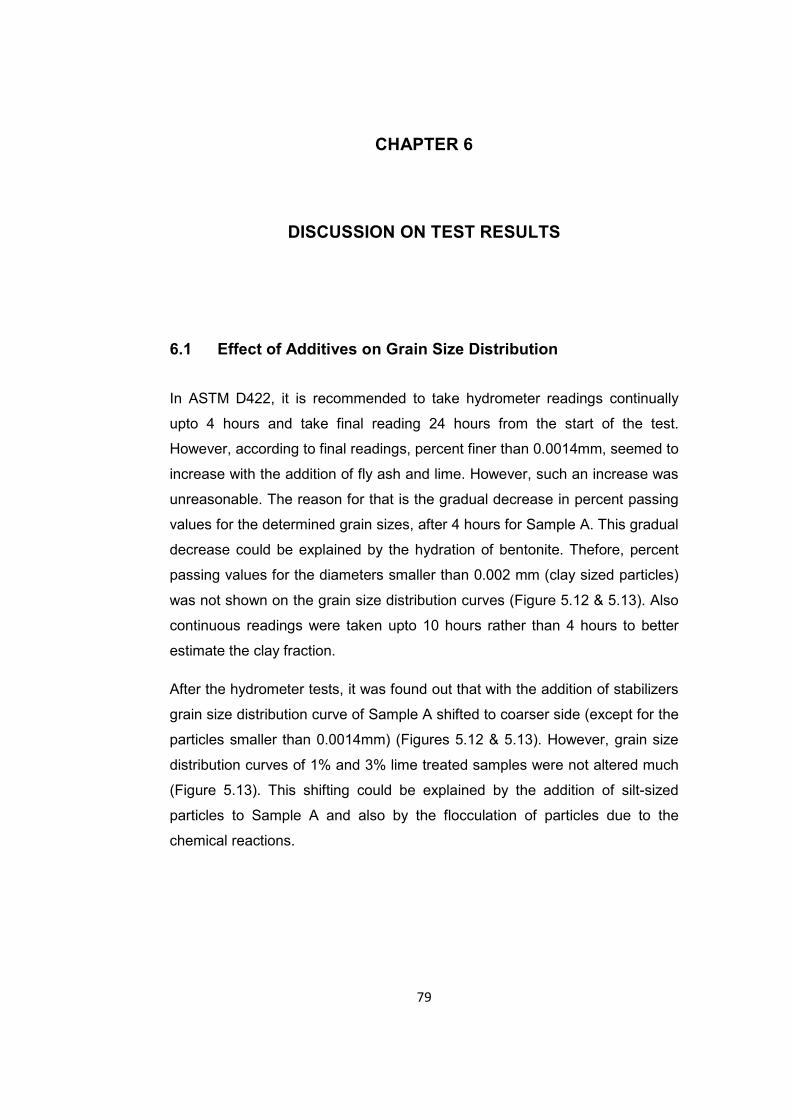
Figure 5.42 EDX Diagram of fly ash within the 5%FA treated sample ............ 77
Page 18
xviii
Figure 5.43 EDX Diagram of fly ash within the 20%FA treated sample (after
cycles) .......................................................................................................... 78
Figure 6.1 Views From 3% lime treated sample after drying ((a)-before first
cycle, (b) – before second cycle) ................................................................... 89
Figure 6.2 View from fungi-shaped heaves occurred in the upper portion of 5%
lime treated sample ....................................................................................... 89
Figure 6.3 SEM views obtained in Ismaiel, (2006) study ................................ 92
Figure A.1 Chemical Analysis Report of Soma Fly Ash ............................... 103
Figure B.1 Swell Amount versus Time Graph for Sample A ......................... 105
Figure B.2 Swell Amount versus Time Graph for 5%FA treated sample with no
curing .......................................................................................................... 106
Figure B.3 Swell Amount versus Time Graph for 5%FA treated sample with
7 days curing ............................................................................................... 107
Figure B.4 Swell Amount versus Time Graph for 5%FA treated sample with 28
days curing .................................................................................................. 108
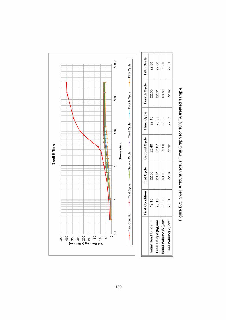
Figure B.5 Swell Amount versus Time Graph for 10%FA treated sample .... 109
Figure B.6 Swell Amount versus Time Graph for 15%FA treated sample .... 110
Figure B.7 Swell Amount versus Time Graph for 20%FA treated sample .... 111
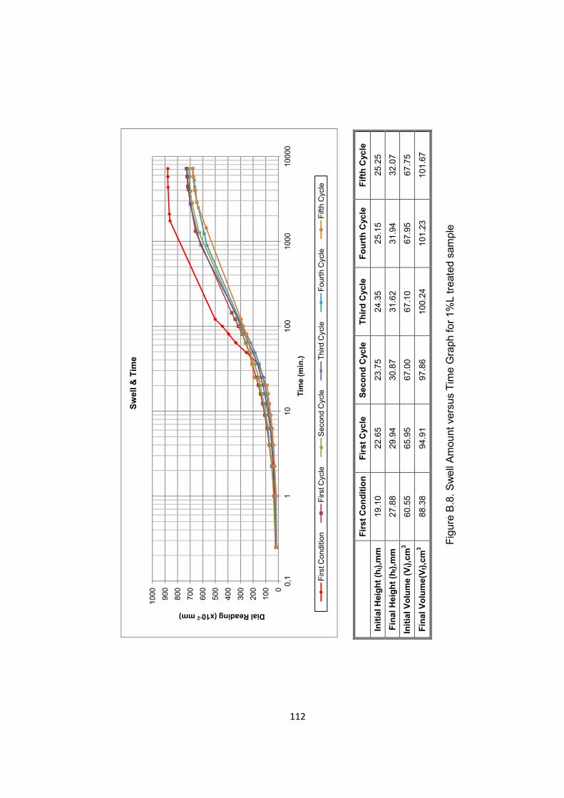
Figure B.8 Swell Amount versus Time Graph for 1%L treated sample ......... 112
Figure B.9 Swell Amount versus Time Graph for 3%L treated sample ......... 113
Figure B.10 Swell Amount versus Time Graph for 5%L treated sample ....... 114
Figure B.11 Swell Amount versus Time Graph for 5%S treated sample ...... 115
Page 19
xix
LIST OF ABBREVIATIONS
ACAA: American Coal Ash Association
ASTM: American Society for Testing and Materials
CH: Clay with high plasticity
EDX: Energy Dispersive X-Ray
F: Fly Ash
FSw-FSh: Full Swell-Full Shrink
FSw-PSh: Full Swell- Partial Shrink
Gs: Specific gravity
Hid = Height at dry state
L: Lime
LL: Liquid limit
Ls: Linear Shrinkage
METU: Middle East Technical University
PI: Plasticity index
PL: Plastic limit
S: Sand
SI: Shrinkage Index
SEM: Scanning Electron Microscope
Page 20
xx
SL: Shrinkage limit
Vid = Volume at dry state
V0 = Initial volume of the sample
∆Hi = Height difference between dry and wet state in a cycle
∆V: Change in volume (with respect to initial volume, V0)
∆Vi = Volume difference between dry and wet state in a cycle
Page 21
1
CHAPTER 1
INTRODUCTION
1.1 General
In arid and semi-arid areas of the world, moisture and rainfall amount varies
considerably in different seasons, structures like small buildings and highways
constructed on expansive soils are encountered with periodic swelling and
shrinkage cycles (Basma, 1996). Cracks and breakups are formed due to
swelling of expansive clays in roads, pavements, building foundations,
irrigation systems, slab-on-grade members channel and reservoir linings,
sewer lines and water lines (Çokça, 2001). In the United States, structures
seated on expansive soils cause an estimated cost of more than 15 billion
dollars due to damage caused from the soil (Al-Rawas, 2006).
Nearly 600 million tons of fly ash is produced each year in all around the
world. In Turkey, 11 power station plants are in operation namely; Afşin-
Elbistan, Çatalağzı, Çayırhan, Kangal, Kemerköy, Orhaneli, Seyitömer, Soma,
Tunçbilek, Yatağan and Yeniköy. The amount of fly ash produced in each year
in these power plants is averagely 16 million ton by the year 2006
(Turker et al., 2009). Although, in many countries rate of utilization of fly ash in
civil engineering applications (mainly in cement production) reaches upto eight
percent of the total produced amount, in Turkey only a small amount is used.
Therefore in Turkey, studies related to utilization of fly ash are needed for the
reduction of environmental problems and financial loss due to the fly ash
deposition in disposal sites (Alkaya, 2009).
Expansive soils’ swelling potantial can be fully eliminated or at least
decreased by using some methods. One of the most widely used stabilization
Page 22
2
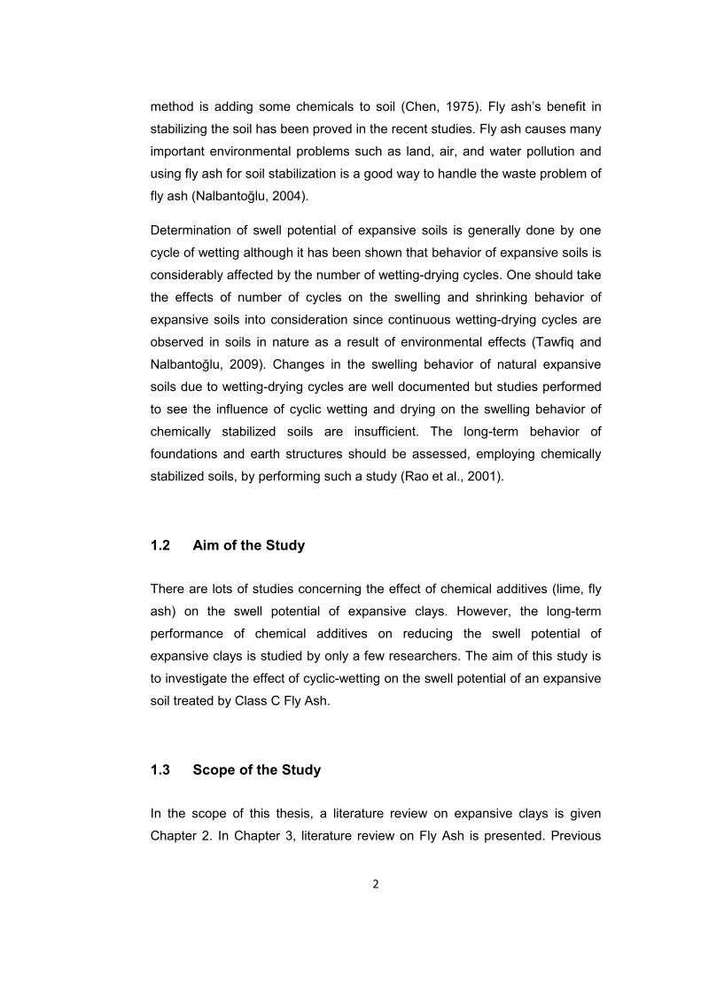
method is adding some chemicals to soil (Chen, 1975). Fly ash’s benefit in
stabilizing the soil has been proved in the recent studies. Fly ash causes many
important environmental problems such as land, air, and water pollution and
using fly ash for soil stabilization is a good way to handle the waste problem of
fly ash (Nalbantoğlu, 2004).
Determination of swell potential of expansive soils is generally done by one
cycle of wetting although it has been shown that behavior of expansive soils is
considerably affected by the number of wetting-drying cycles. One should take
the effects of number of cycles on the swelling and shrinking behavior of
expansive soils into consideration since continuous wetting-drying cycles are
observed in soils in nature as a result of environmental effects (Tawfiq and
Nalbantoğlu, 2009). Changes in the swelling behavior of natural expansive
soils due to wetting-drying cycles are well documented but studies performed
to see the influence of cyclic wetting and drying on the swelling behavior of
chemically stabilized soils are insufficient. The long-term behavior of
foundations and earth structures should be assessed, employing chemically
stabilized soils, by performing such a study (Rao et al., 2001).
1.2 Aim of the Study
There are lots of studies concerning the effect of chemical additives (lime, fly
ash) on the swell potential of expansive clays. However, the long-term
performance of chemical additives on reducing the swell potential of
expansive clays is studied by only a few researchers. The aim of this study is
to investigate the effect of cyclic-wetting on the swell potential of an expansive
soil treated by Class C Fly Ash.
1.3 Scope of the Study
In the scope of this thesis, a literature review on expansive clays is given
Chapter 2. In Chapter 3, literature review on Fly Ash is presented. Previous
Page 23
3
studies related to cyclic-swell shrink behaviour of natural and chemically
stabilized expansive clays are given in Chapter 4. In Chapter 5, 6 and 7 the
experimental works, discussions of the test results and conclusions are
presented respectively.
Page 24
4
CHAPTER 2
2. LITERATURE REVIEW
2.1 Expansive Soils
2.1.1 Clay Mineralogy
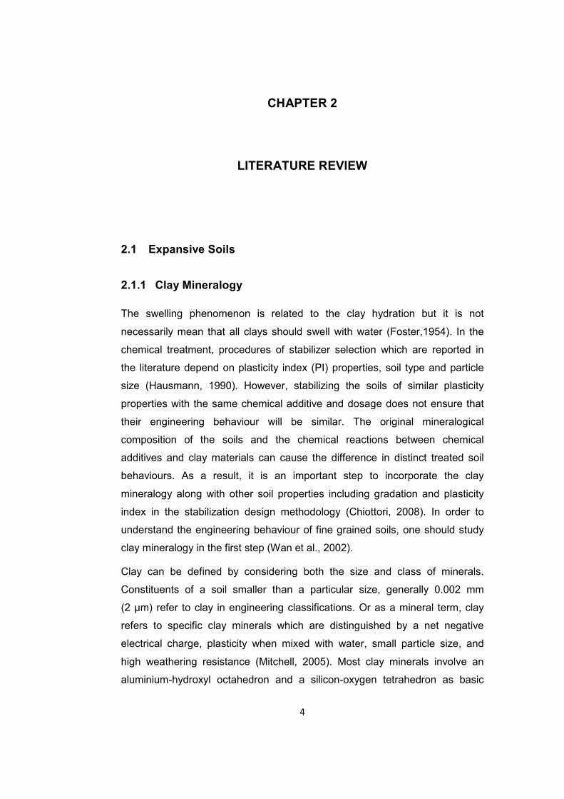
The swelling phenomenon is related to the clay hydration but it is not
necessarily mean that all clays should swell with water (Foster,1954). In the
chemical treatment, procedures of stabilizer selection which are reported in
the literature depend on plasticity index (PI) properties, soil type and particle
size (Hausmann, 1990). However, stabilizing the soils of similar plasticity
properties with the same chemical additive and dosage does not ensure that
their engineering behaviour will be similar. The original mineralogical
composition of the soils and the chemical reactions between chemical
additives and clay materials can cause the difference in distinct treated soil
behaviours. As a result, it is an important step to incorporate the clay
mineralogy along with other soil properties including gradation and plasticity
index in the stabilization design methodology (Chiottori, 2008). In order to
understand the engineering behaviour of fine grained soils, one should study
clay mineralogy in the first step (Wan et al., 2002).
Clay can be defined by considering both the size and class of minerals.
Constituents of a soil smaller than a particular size, generally 0.002 mm
(2 µm) refer to clay in engineering classifications. Or as a mineral term, clay
refers to specific clay minerals which are distinguished by a net negative
electrical charge, plasticity when mixed with water, small particle size, and
high weathering resistance (Mitchell, 2005). Most clay minerals involve an
aluminium-hydroxyl octahedron and a silicon-oxygen tetrahedron as basic
Page 25
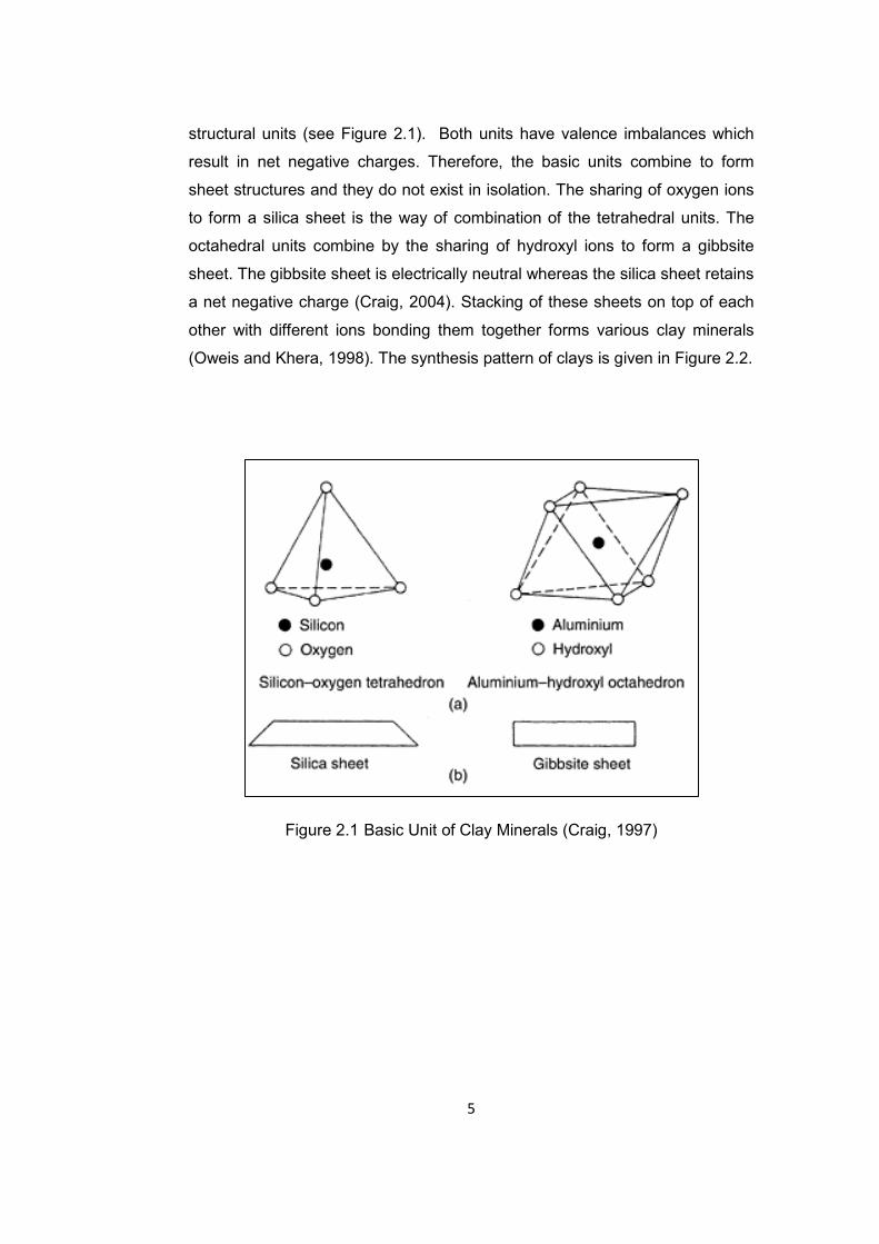
5
structural units (see Figure 2.1). Both units have valence imbalances which
result in net negative charges. Therefore, the basic units combine to form
sheet structures and they do not exist in isolation. The sharing of oxygen ions
to form a silica sheet is the way of combination of the tetrahedral units. The
octahedral units combine by the sharing of hydroxyl ions to form a gibbsite
sheet. The gibbsite sheet is electrically neutral whereas the silica sheet retains
a net negative charge (Craig, 2004). Stacking of these sheets on top of each
other with different ions bonding them together forms various clay minerals
(Oweis and Khera, 1998). The synthesis pattern of clays is given in Figure 2.2.
Figure 2.1 Basic Unit of Clay Minerals (Craig, 1997)
Page 26
6
water + ions
MontmorilloniteIllite
potassium
Kaolinite
Stacked in Various WaysStacked in Various Ways
2:1 Semibasic Unit1:1 Semibasic Unit
Stacked in ionic and covalent bonding to form layers
OctahedralTetrahedral
Repeated to form a sheet
Packed according to charge and geometry
Oxygen or Hydroxyl Various Cations
Figure 2.2 Synthesis pattern of Clay Minerals (modified from Mitchell, 2005)
Crystalline structures (Kaolinite, Illite, and Montmorillonite) could be taken into
account when dividing clay minerals into three main groups.
2.1.1.1 Kaolinite
A single sheet of silica and a single sheet of gibbsite are combined by
relatively strong hydrogen bonding to form kaolinite (Craig, 2004).
Kaolinite yields hydraulic conductivity of a value greater than or equal to 10-6
cm/s. It also has a low activity and low liquid limit (Oweis and Khera, 1998).
Seperation of the layers of Kaolinite is very difficult since they are combined
by strong hydrogen bonds. Thus, it is relatively stable and water cannot
Page 27
7
penetrate between the layers. As a result of this, little swell of kaolinite is
shown on wetting by water (Koteswara, 2011). Structure and scanning
electron micrograph of Kaolinite are given in Figures 2.3 and 2.4, respectively.
Figure 2.3 Structure of Kaolinite (USGS, 2001)
Figure 2.4 Scanning Electron Micrograph of Kaolinite (Murray, 2007)
Page 28
8
2.1.1.2 Illite
Illite has basic structure which consists of a gibbsite sheet between and
combined with two sheets of silica. Partial substitution of silicon by aluminium
is seen in the silica sheet. Bonding that links the combined sheets together is
relatively weak since non-exchangeable potassium ions are present between
the sheets (Craig, 2004). The cation bond of illite is stronger than the water
bond of montmorillonite and weaker than the hydrogen bond of kaolinite
(Koteswara, 2011).
Illite’s hyraulic conductivity is equal to or smaller than 10-7 cm/s and it has a
higher liquid limit than kaolinite (Oweis and Khera, 1998). Illite can be
expansive but problems posed by them are generally not significant (Nelson
and Miller, 1992). Structure and scanning electron micrograph are given in
Figures 2.5 and 2.6, respectively.
Figure 2.5 Structure of Illite (USGS, 2001)
Page 29
9
Figure 2.6 Scanning Electron Micrograph of Illite (source: http://webmineral.com/specimens/picshow.php?id=1284&target=Illite)
2.1.1.3 Montmorillonite
Montmorillonite is a member of the smectite group. It is formed in marine
waters or from weathering of volcanic ash under poor drainage conditions
(Oweis and Khera, 1998). Its basic structure is same with illite. Partial
substitutions of aluminium by magnesium and iron; and silicon by aluminium
are seen in the gibbsite and silica sheets, respectively. A very weak bond,
resulted from being occupied of the spaces between combined sheets by
exchangeable cations (other than potassium) and water molecules, is formed
in the montmorillonite structure (Craig, 2004). The mentioned bond is due to
exchangeable cations and Van der Waals forces. Since the bond is very weak,
it can be broken by water or other cationic or polar organic fluids which enter
between the sheets. An important amount of charge deficiency is observed
due to extensive substitution of silica and alumina. The layers yield much
smaller particles with a very large specific surface and expand much as a
result of easy entrance of water between them. In this clay group,
montmorillonite has the highest liquid limit, activity, and swelling potential
Page 30
10
(Oweis and Khera, 1998). Structure and scanning electron micrograph of
montmorillonite are illustrated in Figures 2.7 and 2.8, respectively.
Figure 2.7 Structure of Montmorillonite (USGS, 2001)
Figure 2.8 Scanning Electron Micrograph of Sodium Montmorillonite
(Murray, 2007)
Page 31
11
2.1.2 Factors Influencing Swelling
According to Nelson and Miller (1992), swelling mechanism of expansive clays
is complex and is influenced by some factors. Many of these factors also
affect physical soil properties (such as plasticity and density) or are affected
by them. Shrink-swell potential of a soil is considered to be influenced by the
factors which can be considered in three different groups. These groups can
be listed as follows:
• Soil Characteristics: Characteristics of soil by which the basic nature
of the internal force field is influenced.
• Environmental Factors: Changes that may occur in the internal force
system can be influenced by some environmental factors. These
factors also influence the shrink-swell potential of a soil.
• State of Stress
The aforementioned factors are given in Tables 2.1, 2.2 and 2.3, in short.
Page 32
12
Table 2.1 Soil Properties that influence shrink-swell potential (Nelson and Miller, 1992)
Clay
Mineralogy
Montmorillonites, vermiculites, and some mixed
layer minerals cause volume changes. Although
Illites and Kaolinites are usually nonexpansive,
these minerals cause volume changes when
particle sizes are extremely fine
Soil Water
Chemistry
Swelling is decreased by the increase in cation
concentration and cation valence. For example,
Mg+2 cations in the soil water would result in less
swelling than Na+ ions.
Soil Suction
Soil suction is an independent effective stress
variable, represented by the negative pore
pressure in unsaturated soils. Soil suction is
related to saturation, gravity, pore size and shape,
surface tension, and electrical and chemical
characteristics of the soil particles and water.
Plasticity
In general, soils that exhibit plastic behavior over
wide ranges of moisture content and that have
high liquid limits have greater potential for swelling
and shrinking. Plasticity is an indicator of swell
potential.
Soil Structure and Fabric
Flocculated clays tend to be more expansive than
dispersed clays. Cemented particles reduce swell.
Fabric and structure are altered by compaction at
higher water content or remolding. Kneading
compaction has been shown to create dispersed
structures with lower swell potential than soils
statically compacted at lower water contents.
Dry Density
Higher densities usually indicate closer particle
spacings, which may mean greater repulsive
forces between particles and larger swelling
potential.
Page 33
13
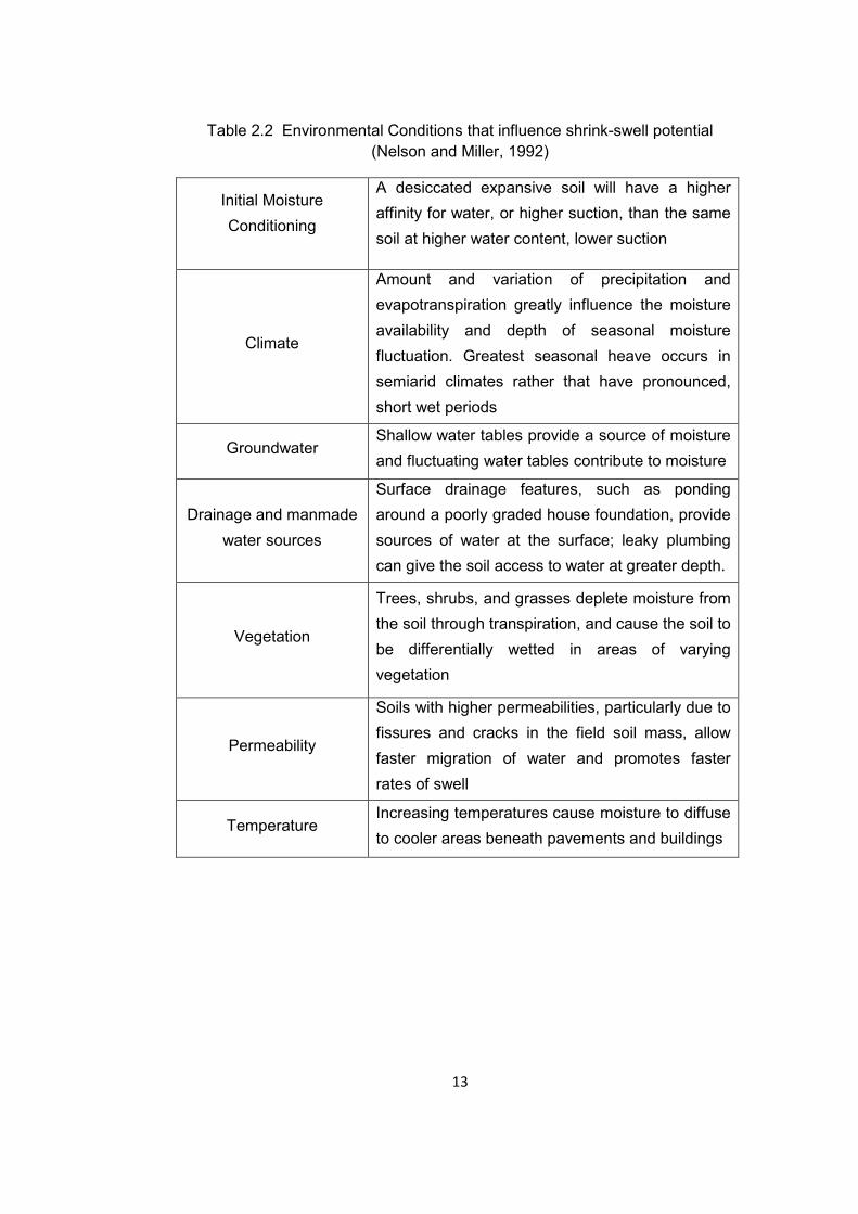
Table 2.2 Environmental Conditions that influence shrink-swell potential (Nelson and Miller, 1992)
Initial Moisture
Conditioning
A desiccated expansive soil will have a higher
affinity for water, or higher suction, than the same
soil at higher water content, lower suction
Climate
Amount and variation of precipitation and
evapotranspiration greatly influence the moisture
availability and depth of seasonal moisture
fluctuation. Greatest seasonal heave occurs in
semiarid climates rather that have pronounced,
short wet periods
Groundwater Shallow water tables provide a source of moisture
and fluctuating water tables contribute to moisture
Drainage and manmade
water sources
Surface drainage features, such as ponding
around a poorly graded house foundation, provide
sources of water at the surface; leaky plumbing
can give the soil access to water at greater depth.
Vegetation
Trees, shrubs, and grasses deplete moisture from
the soil through transpiration, and cause the soil to
be differentially wetted in areas of varying
vegetation
Permeability
Soils with higher permeabilities, particularly due to
fissures and cracks in the field soil mass, allow
faster migration of water and promotes faster
rates of swell
Temperature Increasing temperatures cause moisture to diffuse
to cooler areas beneath pavements and buildings
Page 34
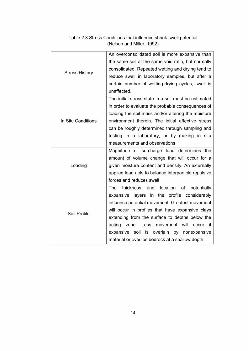
14
Table 2.3 Stress Conditions that influence shrink-swell potential (Nelson and Miller, 1992)
Stress History
An overconsolidated soil is more expansive than
the same soil at the same void ratio, but normally
consolidated. Repeated wetting and drying tend to
reduce swell in laboratory samples, but after a
certain number of wetting-drying cycles, swell is
unaffected.
In Situ Conditions
The initial stress state in a soil must be estimated
in order to evaluate the probable consequences of
loading the soil mass and/or altering the moisture
environment therein. The initial effective stress
can be roughly determined through sampling and
testing in a laboratory, or by making in situ
measurements and observations
Loading
Magnitude of surcharge load determines the
amount of volume change that will occur for a
given moisture content and density. An externally
applied load acts to balance interparticle repulsive
forces and reduces swell
Soil Profile
The thickness and location of potentially
expansive layers in the profile considerably
influence potential movement. Greatest movement
will occur in profiles that have expansive clays
extending from the surface to depths below the
acting zone. Less movement will occur if
expansive soil is overlain by nonexpansive
material or overlies bedrock at a shallow depth
Page 35
15
2.2 Soil Stabilization
2.2.1 Chemical Stabilization
The soil may be removed and replaced with a competent fill where the soil
layer that has expansive characteristics is shallow. The structure is articulately
designed to withstand the expected heave or appropriate soil treatment is
carried out to reduce the heave magnitude in the case where the expansive
layer extends to a larger depth. Removal of the soil and an articulate design of
the structure are expensive works to carry out. Therefore, a practical and
economical approach, stabilization of soil, becomes an attractive alternative in
various cases (Al-Mhaidib and Al-Shamrani, 1996). The oldest and
widespread method of ground improvement is using chemical admixtures for
soil stabilization (Chen, 1975). To stabilize expansive soils, generally, lime,
cement and fly ash are used as admixtures. Physical and chemical conditions
of the natural soil, workability of agent, economic and safety constraints, and
specific conditions of the construction are the factors that affect the application
of these agents (Fang, 1991).
2.2.2 Lime Stabilization
Stabilizing subgrade soil by using lime is a well-known method all over the
world for a long time (Chen, 1975). Three basic chemical reactions occur
when lime and pozzolonic clays are mixed in presence of water. These
reactions are cation exchange and flocculation-agglomeration, cementation
(pozzolanic reaction) and carbonation (Fang, 1991).
Page 36
16
2.2.2.1 Cation Exchange and Flocculation-Agglomeration
The replacement of univalent sodium (Na+) and hydrogen (H+) ions of soil with
divalent (Ca2+) calcium ions of lime results in cation exchange and
flocculation-agglomeration reactions. Clay content and plasticity is bound by
these reactions. Agglomeration reaction of lime and soil is used to destroy
collapsible characteristics of some silts (Fang, 1991).
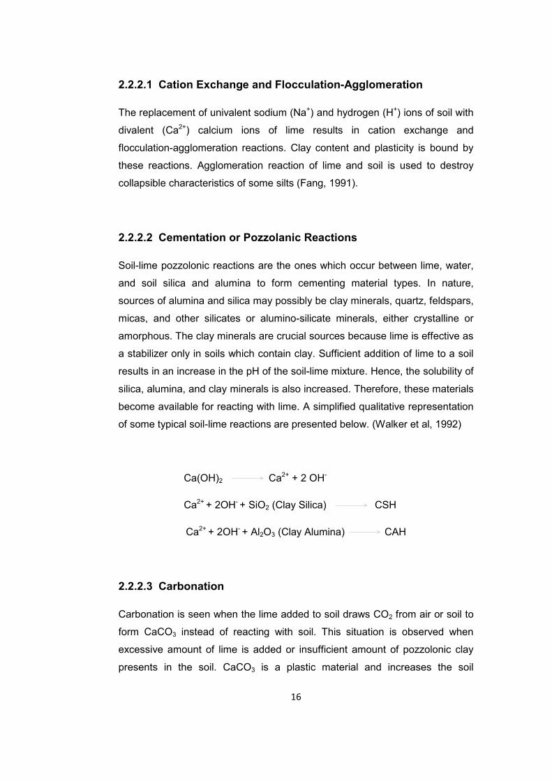
2.2.2.2 Cementation or Pozzolanic Reactions
Soil-lime pozzolonic reactions are the ones which occur between lime, water,
and soil silica and alumina to form cementing material types. In nature,
sources of alumina and silica may possibly be clay minerals, quartz, feldspars,
micas, and other silicates or alumino-silicate minerals, either crystalline or
amorphous. The clay minerals are crucial sources because lime is effective as
a stabilizer only in soils which contain clay. Sufficient addition of lime to a soil
results in an increase in the pH of the soil-lime mixture. Hence, the solubility of
silica, alumina, and clay minerals is also increased. Therefore, these materials
become available for reacting with lime. A simplified qualitative representation
of some typical soil-lime reactions are presented below. (Walker et al, 1992)
Ca(OH)2 Ca2+ + 2 OH-
Ca2+ + 2OH- + SiO2 (Clay Silica) CSH
Ca2+ + 2OH- + Al2O3 (Clay Alumina) CAH
2.2.2.3 Carbonation
Carbonation is seen when the lime added to soil draws CO2 from air or soil to
form CaCO3 instead of reacting with soil. This situation is observed when
excessive amount of lime is added or insufficient amount of pozzolonic clay
presents in the soil. CaCO3 is a plastic material and increases the soil
Page 37
17
plasticity. It also binds lime so that reactions between lime and pozzolanic
materials can not occur. Therefore, beneficial results are not produces in the
case of addition of excessive lime (Fang, 1991).
2.2.3 Fly Ash Stabilization
Fly ash is obtained by collecting the fine residues stemmed from the burning
of pulverized coal in thermal power plants (Ji-Ru and Xing, 2002).
It is endeavoured to make use of fly ash as much as possible since this helps
in abating the disposal problems. Low unit weight, low compressibility and
pozzolanic reactivity are the properties which make fly ash an important agent
for geotechnical engineering. Pozzolanic property makes fly ashes a valuable
stabilizing agent for soils. The pozzolanic reactivity of fly ash is affected by its
reactive silica, free lime content, fineness, carbon content and iron
(Sivapullaiah et al., 1998). Although for lime treatment of soils, pozzolanic
reactions depend on the aluminous and siliceous materials provided by soil,
for class C fly ash, the calcium oxide of the fly ash can react with the
aluminous and siliceous materials of the fly ash itself (Lenol, 2003).
Treatment of expansive soils by using fly ash is shown to be appropriate in the
previous studies (Sivapullaiah et al., 1998; Nalbantoğlu & Güçbilmez, 2001;
Çokça, 2001; Ji-Ru and Xing, 2002; Nalbantoğlu, 2004; Phanikumar and
Sharma, 2007; Zha et al., 2008).
Page 38
18
CHAPTER 3
3. FLY ASH
3.1 General
Ever increasing demand for electricity is met by burning large quantities of
coal in thermal power plants. A residue consisting of inorganic mineral
constituents and partially-burned organic matter remains after the combustion
of coal. The inorganic mineral constituents form ash of which 80% is fly ash
(Sivapullaiah et al., 1998).
Recycling of by-products and wastes becomes an increasingly important
problem for the near future day by day. Considerable amount of coal fly ash is
produced in Turkey and it is accepted as one of the major wastes (Erol et al,
2006). In Turkey, 11 thermal power plants are in operation namely; Afşin-
Elbistan, Çatalağzı, Çayırhan, Kangal, Kemerköy, Orhaneli, Seyitömer, Soma,
Tunçbilek, Yatağan and Yeniköy. The amount of fly ash produced in each year
in these power plants is averagely 16 million tons by the year 2006 (Turker et
al., 2009).
Deposition of these wastes could cause air, water and soil pollution that have
negative impacts on human health. Representative figure showing coal ash
pollution chain prepared by Greenpeace (2010) is given below (Figure 3.1).
Page 39
19
Fig
ure
3.1
Coal A
sh P
ollu
tion C
hain
(G
reenpeace
,2010)
Page 40
20
3.2 Factors that influence Fly Ash Properties
The fly ash properties are influenced by several factors and it could change in
the same power plant even in the same day because of the change in loading
conditions (Görhan, 2009). The primary affecting factors include the coal
source and boiler & emission control design. The mineralogy and specific fly
ash sources’ properties are affected by these factors (Mackiewicz and
Ferguson, 2005).
3.2.1 Coal Source
The type and amount of inorganic matter within the coal and the constituents
within the fly ash are dictated by the coal source. The produced ash does not
show self-cementing properties since bituminous and many lignite coals have
low concentrations of calcium compounds. Typically, higher concentrations of
calcium carbonate is observed in subbituminous coals and the produced fly
ash contains 20 to 30% calcium compounds (Mackiewicz and Ferguson,
2005).
3.2.2 Boiler and Emission Control Design
As the chemical constituents of a particular fly ash are dictated by the coal
source, crystalline compounds existing in fly ash are also highly influenced by
boiler and emission control design as well as plant operation.The rate at which
the fused particles are cooled dictated the fly ash hydration characteristics.
The inorganic matter existing in the coal is fused and transported from the
combustion chamber during combustion. These small particles are suspended
in the exhaust gases. Rapid cooling of the mentioned particles results in a
noncrystalline (glassy) or amorphous fly ash structure. Whereas, when the
particles are cooled at a slower rate, the structure of the produced fly ash is
more crystalline. As the self-cementing characteristics of the fly ash is
provided by the crystalline compounds, the degree of crystallinity, which in
Page 41
21
turn determines the specific fly ash sources’ hydration characteristics, is
influenced by the boiler and emission control design as well as plant operation
(Mackiewicz and Ferguson, 2005).
3.3 Classification of Fly Ashes
According to ASTM C-618-08a (Standard Specification for Coal Fly Ash and
Raw or Calcined Natural Pozzolan for Use in Concrete), fly ashes are divided
into two classes. These classes are named as Class F and Class C and they
are explained below.
• Class F: Production of Class F fly ash is typically made by burning
bituminous coal or anthracite. It can also be produced from lignite and
subbituminous coal. Pozzolanic properties are exhibited by this class of
fly ash but it has no self-cementing properties. This material can be
used for many soil stabilization applications by adding some activators
(lime etc.) into fly ash to obtain cementitious properties.
• Class C: Typically, burning of lignite or subbituminous coal results in
Class C type of fly ash. This class can also be produced from
anthracite or bituminous coal. Total calcium content, expressed as
calcium oxide (CaO), of this type of fly ash is more than 10%. In
addition to having pozzolonic properties, Class C fly ash also has some
cementitious properties.
In this study, Fly Ash taken from Soma Thermal Power Plant is used.
3.4 Soma Thermal Power Plant
Soma Thermal Power Plant is located in Manisa Province, Soma District. It is
90 and 130km away from Manisa and İzmir respectively (Direskeneli, 2007).
With an installed capacity of 1034 MW, Soma thermal power plant consumes
30,000 tons of low-quality lignite obtained from the reserves of Soma basin
Page 42
22
and approximately 12,000 tons of fly ash is produced per day. Conveyor belts
which are nearly 10 km in length are utilized to transport the solid waste to the
disposal site. Spreading of ash by wind is prevented by damping the solid
waste by using nozzle on the conveyor. Furthermore, water is added to the
waste at the disposal site so that a slurry pond is formed. Approximately 7
liters of water is needed to sluice 1 kg of coal ash obtained from the Soma
thermal power plant (Baba and Kaya, 2003).
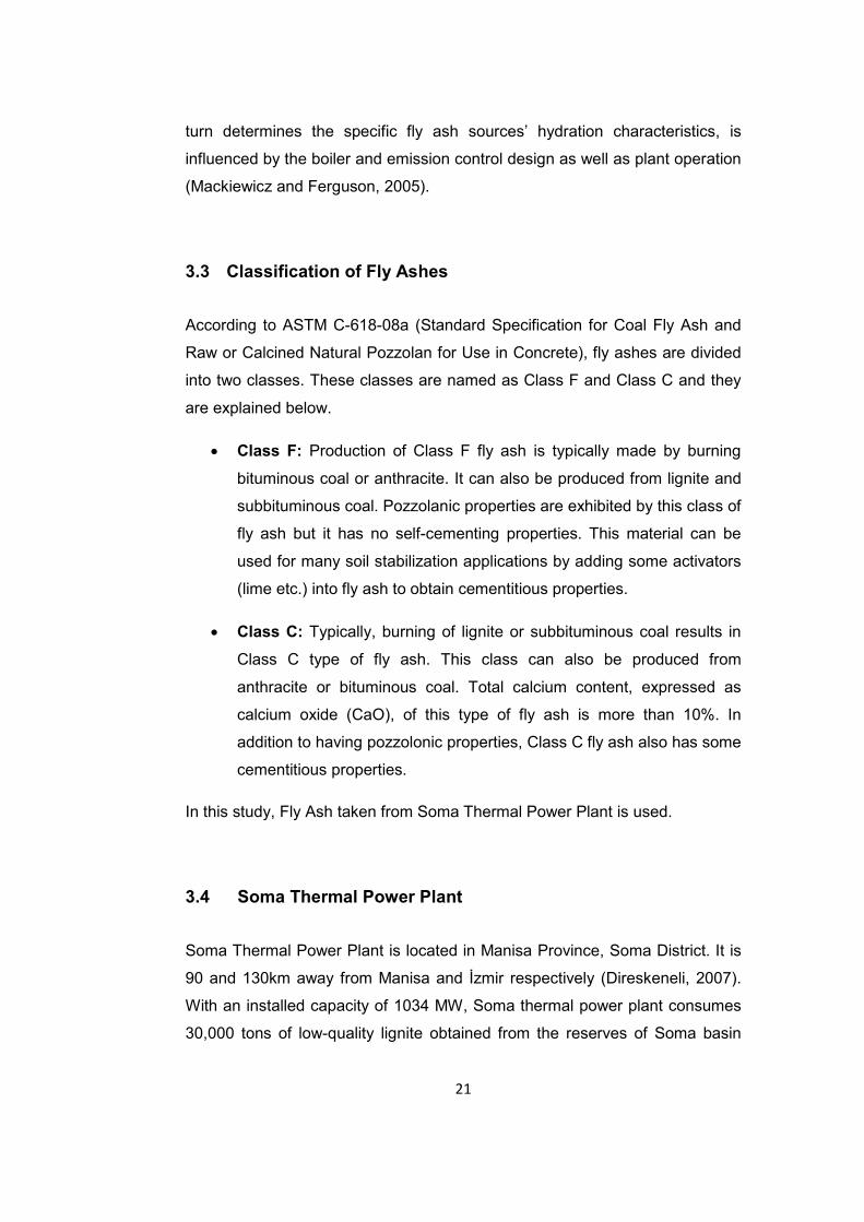
In Turkey, ponds are not frequently used since they require considerable
amount of area and they cause water quality deterioration of sluicing waters.
However, Soma thermal power plant has a large ash pond. This pond is used
as the ultimate waste disposal site (Figure 3.2) (Baba and Kaya, 2003).
Figure 3.2 Ash Disposal Site of Soma Thermal Power Plant (Baba and Kaya, 2003)
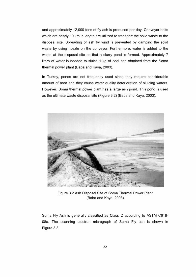
Soma Fly Ash is generally classified as Class C according to ASTM C618-
08a. The scanning electron micrograph of Soma Fly ash is shown in
Figure 3.3.
Page 43
23
Figure 3.3 Scanning Electron Micrograph of Soma Fly Ash (Çelik, 2004)
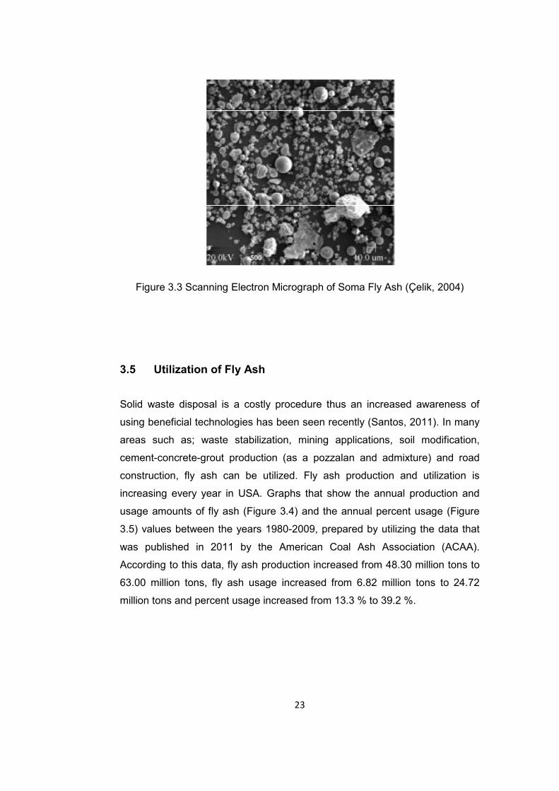
3.5 Utilization of Fly Ash
Solid waste disposal is a costly procedure thus an increased awareness of
using beneficial technologies has been seen recently (Santos, 2011). In many
areas such as; waste stabilization, mining applications, soil modification,
cement-concrete-grout production (as a pozzalan and admixture) and road
construction, fly ash can be utilized. Fly ash production and utilization is
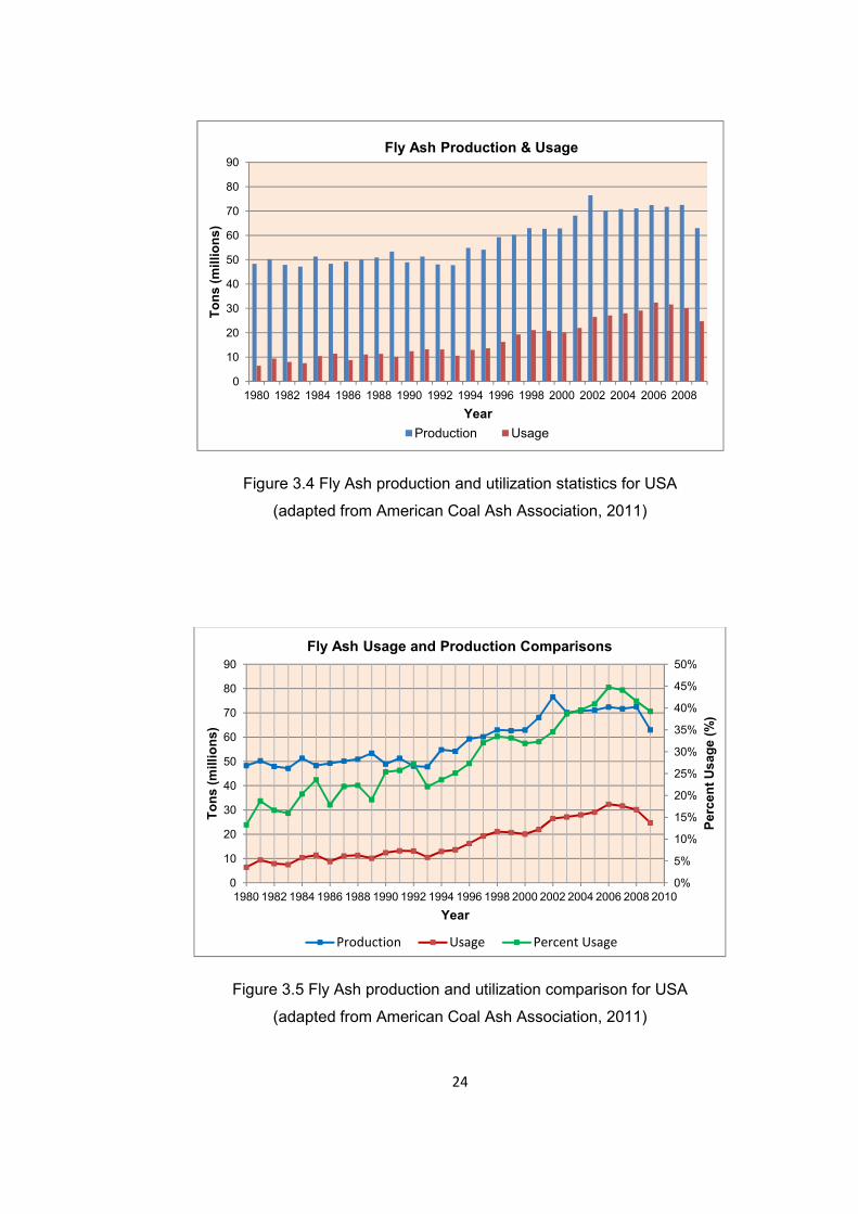
increasing every year in USA. Graphs that show the annual production and
usage amounts of fly ash (Figure 3.4) and the annual percent usage (Figure
3.5) values between the years 1980-2009, prepared by utilizing the data that
was published in 2011 by the American Coal Ash Association (ACAA).
According to this data, fly ash production increased from 48.30 million tons to
63.00 million tons, fly ash usage increased from 6.82 million tons to 24.72
million tons and percent usage increased from 13.3 % to 39.2 %.
Page 44
24
Figure 3.4 Fly Ash production and utilization statistics for USA
(adapted from American Coal Ash Association, 2011)
Figure 3.5 Fly Ash production and utilization comparison for USA
(adapted from American Coal Ash Association, 2011)
0
10
20
30
40
50
60
70
80
90
1980 1982 1984 1986 1988 1990 1992 1994 1996 1998 2000 2002 2004 2006 2008
To
ns
(m
illi
on
s)
Year
Fly Ash Production & Usage
Production Usage
0%
5%
10%
15%
20%
25%
30%
35%
40%
45%
50%
0
10
20
30
40
50
60
70
80
90
1980 1982 1984 1986 1988 1990 1992 1994 1996 1998 2000 2002 2004 2006 2008 2010
Pe
rce
nt
Us
ag
e(%
)
To
ns
(m
illi
on
s)
Year
Fly Ash Usage and Production Comparisons
Production Usage Percent Usage
Page 45
25
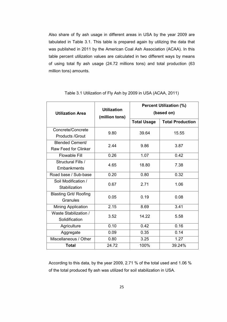
Also share of fly ash usage in different areas in USA by the year 2009 are
tabulated in Table 3.1. This table is prepared again by utilizing the data that
was published in 2011 by the American Coal Ash Association (ACAA). In this
table percent utilization values are calculated in two different ways by means
of using total fly ash usage (24.72 millions tons) and total production (63
million tons) amounts.
Table 3.1 Utilization of Fly Ash by 2009 in USA (ACAA, 2011)
Utilization Area Utilization
(million tons)
Percent Utilization (%)
(based on)
Total Usage Total Production
Concrete/Concrete
Products /Grout 9.80 39.64 15.55
Blended Cement/
Raw Feed for Clinker 2.44 9.86 3.87
Flowable Fill 0.26 1.07 0.42
Structural Fills /
Embankments 4.65 18.80 7.38
Road base / Sub-base 0.20 0.80 0.32
Soil Modification /
Stabilization 0.67 2.71 1.06
Blasting Grit/ Roofing
Granules 0.05 0.19 0.08
Mining Application 2.15 8.69 3.41
Waste Stabilization /
Solidification 3.52 14.22 5.58
Agriculture 0.10 0.42 0.16
Aggregate 0.09 0.35 0.14
Miscellaneous / Other 0.80 3.25 1.27
Total 24.72 100% 39.24%
According to this data, by the year 2009, 2.71 % of the total used and 1.06 %
of the total produced fly ash was utilized for soil stabilization in USA.
Page 46
26
CHAPTER 4
4. PREVIOUS STUDIES ON CYCLIC SWELL-SHRINK BEHAVIOUR OF SOILS
4.1 General
In the previous studies two methods have been used for determining the cyclic
swell-shrink behavior of expansive soils. These are the full swell-full shrink
and full swell-partial shrink (Güney et al., 2007)
Full Swell-Full Shrink: Samples are allowed to swell until the primary swell
completed or no more swell is observed, and dried fully or until the water
content comes below the shrinkage limit.
Full Swell-Partial Shrink: Samples are allowed to swell until the primary
swell completed or no more swell is observed, and dried to their initial
moisture content.
4.2 Studies on Nonstabilized Soils
Day, (1994) performed cyclic swell-shrink tests on silty clay soil with liquid and
plastic limits of 46% and 24%, respectively. Full swell-full shrink tests were
conducted where the soils were allowed to dry below their shrinkage limit. The
author found out that full swell-full shrink cycles caused an increase in swell
potential and this increase was explained by destruction of the floocculated
structure of clay and formation of more expansive and permeable soil having a
dispersed structure.
Page 47
27
In the study performed by Al-Homoud et al, (1995), expansive characteristics
of soils which were exposed to swell-shrink cycles were investigated. Tests
were conducted on six different soils with liquid, plastic, and shrinkage limits
varying between 65-90%, 15-40% and 10-20%, respectively. During the
experiments full swell-partial shrink method were used. The results showed
that as the number of cycle increases, swell potential decreases. Furthermore,
it was noted that first cycle caused the maximum reduction in swelling
potential and swell percent reached to equilibrium after conducting 4-5 cycles.
The authors explained the swell reduction with the soil particles’
rearrangement.
Basma, (1996) studied on four different soils to determine the effect of cyclic
swell–shrink on expansive soils. Both partial and full shrink methods were
applied. For partial shrink, samples were allowed to dry at room temperature,
and for full shrink, samples were exposed to sunlight. The results of the
experiments showed that an increase in the swell potential was observed after
full shrink and a decrease was seen after partial shrink. Swell potential came
to a constant value at the end of 4-5 cycles. Apart from the other researchers,
Basma (1996) performed ultra sound investigation test on samples, and found
out that void ratio of samples that were exposed to full shrink cycles increased
and that of ones which were exposed to partial shrink cycles decreased.
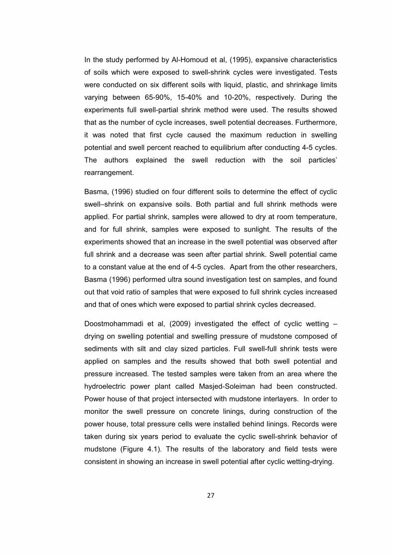
Doostmohammadi et al, (2009) investigated the effect of cyclic wetting –
drying on swelling potential and swelling pressure of mudstone composed of
sediments with silt and clay sized particles. Full swell-full shrink tests were
applied on samples and the results showed that both swell potential and
pressure increased. The tested samples were taken from an area where the
hydroelectric power plant called Masjed-Soleiman had been constructed.
Power house of that project intersected with mudstone interlayers. In order to
monitor the swell pressure on concrete linings, during construction of the
power house, total pressure cells were installed behind linings. Records were
taken during six years period to evaluate the cyclic swell-shrink behavior of
mudstone (Figure 4.1). The results of the laboratory and field tests were
consistent in showing an increase in swell potential after cyclic wetting-drying.
Page 48
28
Figure 4.1 Total pressure cells data for the Power House linings of Masjed-Soleiman Hydroelectric Power Plant Project (Doostmohammadi, 2009)
Tawfiq & Nalbantoğlu, (2009), studied the effect of the cyclic wetting and
drying on the swelling behavior of a natural expansive soil with liquid limit and
plasiticity index values of 64% and 36%, respectively. During the experiments
both full swell-full shrink and full swell-partial shrink methods were applied.
Results of the experiments showed that swell potential increased after full
swell-full shrink cycles and decreased after full swell-partial shrink cycles.
Authors explained the swell potential increase after full shrink cycles with the
decrease in the water content and development of macro cracks at the end of
the second cycle that allowed water to penetrate into soil pores. Also, swell
potential decrease due to partial shrink method was explained by the high
water content existing before the wetting procedure. For the full swell –full
shrink and full swell-partial shrink cycles swell potential come into equilibrium
after the fifth and the first cycle, respectively (Figure 4.2).
Page 49
29
Figure 4.2 Effect of full swell-full shrink and full swell-partial shrink on swell potential of an expansive soil (Tawfiq & Nalbantoğlu, 2009)
Tripathy & Rao, (2009) carried out cyclic swell–shrink tests under 50 kPa of
surcharge pressure on a compacted expansive clay with liquid limit and
plasticity index of 100% and 58%, respectively. In this study, both of the
shrinkage methods were used as that of Tawfiq & Nalbantoğlu, (2009) studies.
Increase in swell potential was observed after full shrink cycles even after the
first cycle and swell potential decreased for partial shrink cycles. Swell
potential came into equilibrium after five or more cycles.
Türköz, (2009) conducted tests on an expansive soil obtained by mixing
different percentages of bentonite with high plasticity Silty Clay to determine
the effect of wetting-drying on microstructure. Samples were allowed to swell
fully and than dried to shrinkage limit. Only the swell values were presented in
the study. Swell percentages could not be presented due to the deformations
occurred on the surface of samples during drying. The results showed that
after each cycle, swell amount decreased. The reduction was explained by the
flocculation of particles.
Page 50
30
In addition to these researchers, the studies of Popesco (1980) and Osipov et
al. (1987) on nonstabilized soils showed that full swell-full shrink cycles
caused an increase in the swelling potential of soils and also the studies of
Chen (1965), Chen et al. (1985) and Dif and Blumel (1991) showed that
reduction occurred in swelling potential of expansive soils that exposed to full
swell-partial shrink cycles (Basma, 1996).
The summary of the swell-shrink procedures applied by different researchers
to see the effect of wetting-drying cycles on swelling properties of non-
stabilized expansive soils is presented in Table 4.1
The previous studies indicate that there occurs an increase in swelling
potential of expansive soils that were exposed to full swell-full shrink cycles. A
reduction in swell potential is seen for the soils that were exposed to full swell-
partial shrink cycles.
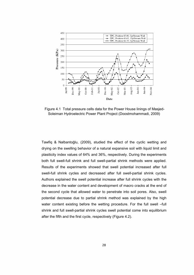
Table 4.1 Swell-Shrink Procedures applied on nonstabilized expansive soils in previous studies by different researchers
Authors
Swell-
Shrink Method
Swell
Procedure
Shrinkage
Procedure
Day,(1994) FSw-FSh*
At least until
primary swell
completed
(1.5 days)
Exposed to sunshine
at summer
(2.5 days)
Al-Homoud et al,
(1995) FSw-PSh**
At least until
primary swell
completed
(at least 40 hrs)
Dried at laboratory
environment
(1 day)
Basma, (1996)
FSw-PSh Until full swell
completed (24
hours)
Dried at room
temperature
( 1 day)
FSw-FSh Exposed to sunshine
(1.5 days)
Page 51
31
Table 4.1 Swell-Shrink Procedures applied on nonstabilized expansive soils in previous studies by different researchers (continued)
Authors Swell-Shrink
Method
Swell Procedure
Shrinkage Procedure
Doostmohammadi
et al, (2009) FSw-FSh
Until full swell
completed
Dried at 40°C until
reaching of a constant
strain value
Tawfiq &
Nalbantoğlu, 2009
FSw-PSh Until full swell
completed
(4 days)
Dried at 40±3°C)
(3 days and 8 days for
partial and full
shrinkage) FSw-FSh
Tripathy & Rao,
(2009)
FSw-PSh Until full swell
completed
( 3 days)
Dried at 40±5°C
(0.5- 1.0 day)
FSw-FSh Dried at 40±5°C
(4 days)
Türköz (2009) FSw-FSh
Until 91% of full
swell completed
(1 day)
Dried at 105 °C
( 1 day)
*Full Swell-Full Shrink ** Full Swell-Partial Shrink
4.3 Studies on Stabilized Soils
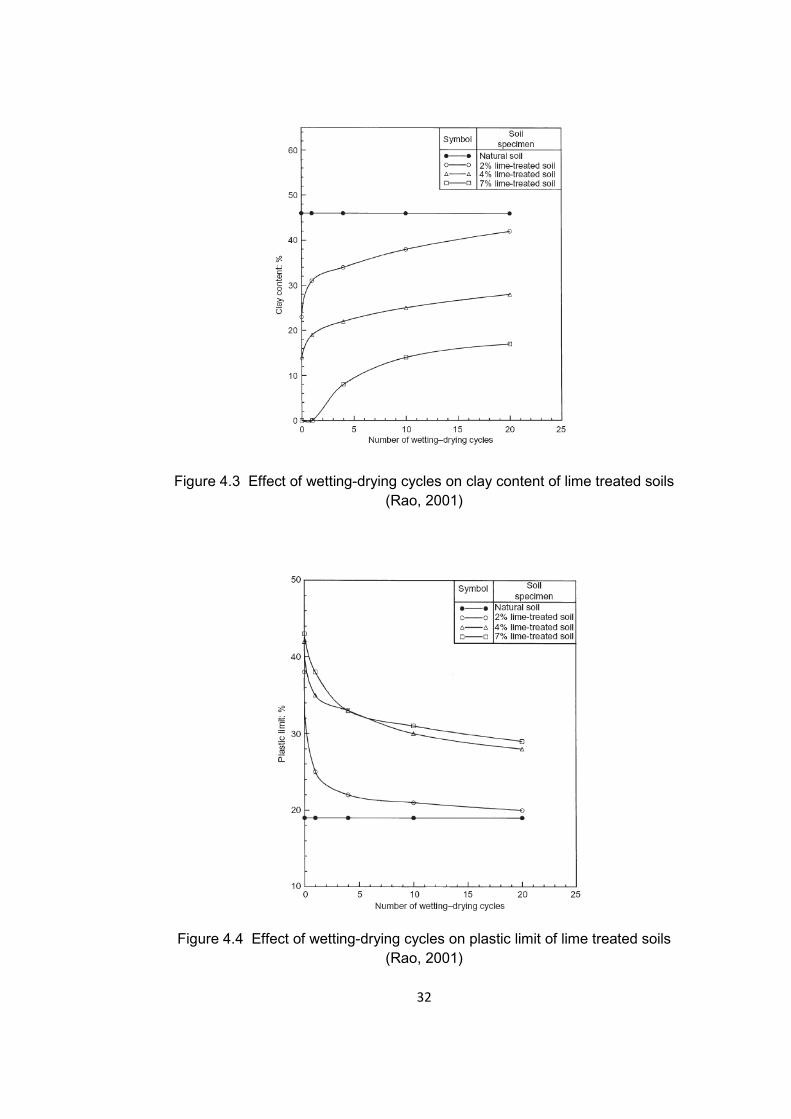
Rao et al, (2001) studied the effect of wetting-drying cycles on the lime-treated
soil’s index properties. Hydrometer and Atterberg limit tests were applied to
lime-treated soil. Hydrated lime was used in the experiments with the
percentages 2%, 4% and 7%. Full swell-full shrink method was used and
specimens were exposed to 20 wetting – drying cycles during the tests. At the
end of the experiments, clay content and liquid limit increased and plastic limit
and shrinkage limit of treated samples decreased (Figures 4.3 and 4.4). The
author explained the corresponding increase and reduction in the index
properties by breakdown of cementation and flocculation of particles and by
the increase in the thickness of diffuse double layer.
Page 52
32
Figure 4.3 Effect of wetting-drying cycles on clay content of lime treated soils (Rao, 2001)
Figure 4.4 Effect of wetting-drying cycles on plastic limit of lime treated soils (Rao, 2001)
Page 53
33
Another study was also performed by Rao et al, (2001) on lime-treated
expansive soils. This time, the effect of cyclic wetting – drying cycles on swell
potential of lime treated expansive soils was investigated. Full swell-full shrink
method was used as in the previous study. The resuls of the experiments
indicated that the effect of lime treatment was partially reduced after four
wetting-drying cycles.
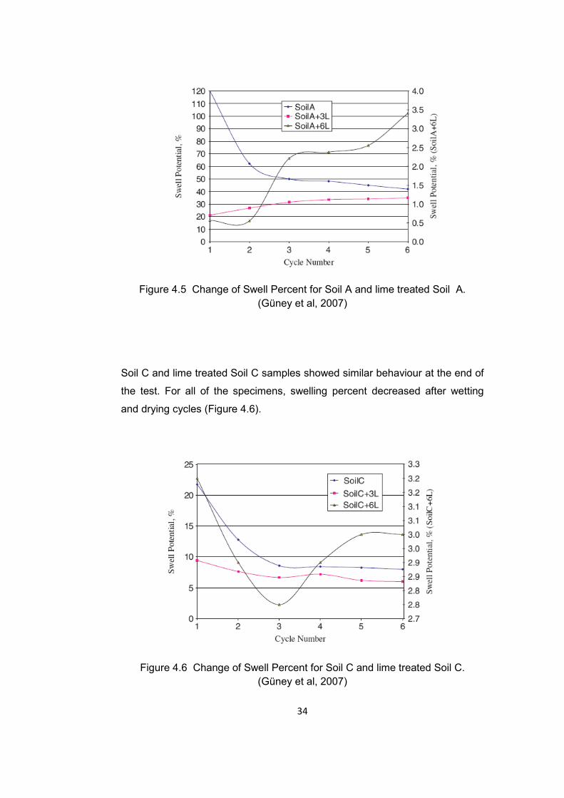
Güney et al, (2007) also conducted cyclic swell – shrink tests to determine the
long term behavior of lime-treated clayey soils. During the tests, samples were
dried to their initial moisture content. Tests were carried out on three different
soils. During the study two different proportions of lime; 3% and 6%, were
used. Properties of the materials that were used in this study are presented in
Table 4.2.
Table 4.2 Properties of the materials used in Güney et al, (2007) studies.
Sample Liquid Limit
(%)
Plastic Limit
(%)
Plasticity İndex
(%)
Shrinkage Limit
(%)
Soil A 385 35 350 23
Soil A + 3L 360 45 315 26
Soil A + 6L 255 57 198 29
Soil B 168 28 140 27
Soil B+ 3L 160 37 123 30
Soil B + 6L 140 45 95 35
Soil C 115 45 70 25
Soil C + 3L 104 49 55 41
Soil C + 6L 103 50 53 58
At the end of the tests, swell potential of Soils A and B reduced in the first
cycle and reached to equilibrium after the fourth cycle. However, swell
potentials of 3% and 6% lime treated soils increased (Figure 4.5).
Page 54
34
Figure 4.5 Change of Swell Percent for Soil A and lime treated Soil A. (Güney et al, 2007)
Soil C and lime treated Soil C samples showed similar behaviour at the end of
the test. For all of the specimens, swelling percent decreased after wetting
and drying cycles (Figure 4.6).
Figure 4.6 Change of Swell Percent for Soil C and lime treated Soil C. (Güney et al, 2007)
Page 55
35
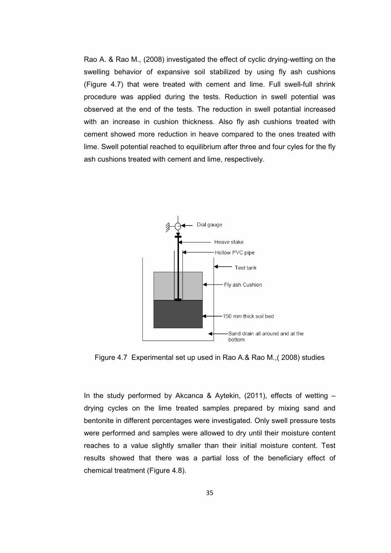
Rao A. & Rao M., (2008) investigated the effect of cyclic drying-wetting on the
swelling behavior of expansive soil stabilized by using fly ash cushions
(Figure 4.7) that were treated with cement and lime. Full swell-full shrink
procedure was applied during the tests. Reduction in swell potential was
observed at the end of the tests. The reduction in swell potantial increased
with an increase in cushion thickness. Also fly ash cushions treated with
cement showed more reduction in heave compared to the ones treated with
lime. Swell potential reached to equilibrium after three and four cyles for the fly
ash cushions treated with cement and lime, respectively.
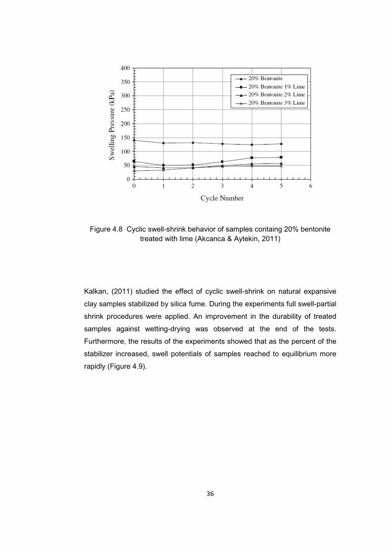
Figure 4.7 Experimental set up used in Rao A.& Rao M.,( 2008) studies In the study performed by Akcanca & Aytekin, (2011), effects of wetting –
drying cycles on the lime treated samples prepared by mixing sand and
bentonite in different percentages were investigated. Only swell pressure tests
were performed and samples were allowed to dry until their moisture content
reaches to a value slightly smaller than their initial moisture content. Test
results showed that there was a partial loss of the beneficiary effect of
chemical treatment (Figure 4.8).
Page 56
36
Figure 4.8 Cyclic swell-shrink behavior of samples containg 20% bentonite
treated with lime (Akcanca & Aytekin, 2011)
Kalkan, (2011) studied the effect of cyclic swell-shrink on natural expansive
clay samples stabilized by silica fume. During the experiments full swell-partial
shrink procedures were applied. An improvement in the durability of treated
samples against wetting-drying was observed at the end of the tests.
Furthermore, the results of the experiments showed that as the percent of the
stabilizer increased, swell potentials of samples reached to equilibrium more
rapidly (Figure 4.9).
Page 57
37
Figure 4.9 Cyclic swell-shrink behavior of expansive soil stabilized with
silica fume (Kalkan, 2011)
The summary of the swell-shrink procedure of the authors that studied the
effect of wetting-drying cycles on swelling properties of stabilized expansive
soils is presented in Table 4.3.
Page 58
38
Table
4.3
Sw
ell-
Shrink
Pro
cedure
s applie
d o
n s
tabili
zed e
xpan
sive
soils
in p
revi
ous
studie
s by
diff
ere
nt re
searc
hers
Au
tho
rs
Sw
ell-
Sh
rin
k
Meth
od
S
well P
roced
ure
S
hri
nkag
e P
roce
du
re
Ad
dit
ive T
ype
(Perc
en
t (%
))
Co
nclu
sio
n
Rao e
t al.
(2001)
FS
w-F
Sh
U
ntil
full
swell
com
ple
ted (
2 d
ays
)
Dried a
t 45°C
by
a
hot
circ
ula
tor
( 2
days
)
Lim
e
(2%
,4%
and 7
%)
Sw
ell
Pote
ntia
l and
Cla
y C
onte
nt
incr
ease
d
Güney
et al.
(2007)
FS
w-P
Sh
At
least
until
prim
ary
swell
com
ple
ted (6
0
hours
)
Air-d
ried a
t 24°C
until
l
initi
al m
ois
ture
conte
nt
reach
ed
Lim
e
(3%
and 6
%)
Sw
ell
Pote
ntia
l
incr
ease
d for
two
treate
d s
am
ple
s and
decr
ease
d for
one
Rao A
. &
Rao
M.,
(2008)
FS
w-F
Sh
Until
there
was
no
chang
e in
dia
l gaug
e
for
3 c
onse
cutiv
e d
ay
Until
there
was
no
chang
e in
thic
kness
for
3 c
onse
cutiv
e d
ay
Fly
Ash
Cush
ions
(tre
ate
d w
ith li
me
and c
em
ent)
Sw
ell
Pote
ntia
l
decr
ease
d
Akc
anca
&
Ayt
eki
n, (2
011)
FS
w-P
Sh
Until
sw
elli
ng
pre
ssure
reach
ed
(7 d
ays
)
Dried a
t 35±5°C
to a
mois
ture
conte
nt a li
ttle
bit
belo
w in
itial m
ois
ture
conte
nt (1
day)
Lim
e
(1%
,2%
and 3
%)
Sw
ell
Pre
ssure
incr
ease
d
Kalk
an, (2
011)
FS
w -
PS
h
Until
l full
swell
com
ple
ted
(ove
r 2 d
ays
)
Air-d
ried a
t 22°C
until
initi
al m
ois
ture
conte
nt
reach
ed (
5 d
ays
)
Sili
ca F
um
e
(10%
,20%
,25 a
nd
30%
)
Sw
ell
Pote
ntia
l
decr
ease
d
38
Page 59
39
The previous studies on stabilized expansive soils show that although
beneficiary effect of silica fume and fly ash cushions in reducing the swell
potential was preserved after cyclic swell-shrink cycles, that of lime was
partially lost mostly. However, in the studies conducted by Güney et al. (2007)
on three different soils treated with same lime type and percentages, the swell
potentials of two lime treated soil increased whereas a decrease in swell
potential observed in the remaining one. Therefore, there could be a decrease
or an increase in the swell potantial after cyclic-swell shrink tests for lime
treated soils. In short, further studies should be conducted on chemically
treated expansive soils for better estimation of the long-term behavior.
Page 60
40
CHAPTER 5
5. EXPERIMENTAL WORKS
5.1 Purpose
The aim of this study is to investigate the effects of addition of Class C Fly Ash
on atterberg limits, grain size distribution, swell percentage and then to
investigate the effect of cyclic swell-shrink on swell percentage of an
expansive soil stabilized by Class C Fly Ash.
5.2 Materials
Bentonite, kaolinite, Class C fly ash, lime and sand were used in this study.
Bentonite: Na-Bentonite was used in this study, which was the product of
Karakaya Bentonite Factory, located in Ankara (Figure 5.1).
Kaolinite: Kaolinite was product of Kale Maden Industrial Raw Materials
Industry & Trade Co. This material was grounded into fine grains in METU
Civil Engineering Department Transportation Laboratory and sieved through
# 40 sieve before usage (Figure 5.1).
Fly Ash: Class C Fly Ash from Soma Thermal Power Plant was utilized. It was
taken from Ilion Cement Construction Industry and Trade Co. as a bagged
material (dry). This material sieved through # 40 sieve before usage (Figure
5.1). Specific gravity of Fly Ash is 2.56. Minealogical composition of Fly Ash
was determined by X-Ray diffraction method performed in General Directorate
Page 61
41
of Mineral Research and Exploration (Appendix A). Chemical analysis of the
Fly Ash is presented in Table 5.1.
Lime: Hydrated lime was taken from Baştaş Cement Trade Inc. This material
passed through # 40 sieve before usage (Figure 5.1). Specific gravity of Lime
is 2.52. Chemical contents of lime that obtained from supplier is given in Table
5.1.
Sand: Sand with a gradation smaller than 0.425mm (passing through #40
sieve) was used.
Table 5.1 Chemical Composition of Fly Ash and Lime
Composition (%) Fly Ash Lime
SiO2 (Silica) 38.10 0.58
Al2O3 (Alumina) 16.55 0.38
TiO2 (Titanium Dioxide) 0.70 *
Fe2O3 (Ferric Oxide) 4.10 0.11
CaO (Calcium Oxide) 31.45 67.76
MgO (Magnesium Oxide) 1.35 2.20
Na2O (Sodium Oxide) 0.35 *
K2O (Potassium Oxide) 1.40 *
P2O5 (Phosphorus Oxide) 0.20 *
MnO (Manganese Oxide) 0.10 *
Loss on Ignition 0.45 *
*Not determined
Figure 5.1. Views from Materials (1-kaolinite, 2-bentonite, 3-fly ash, 4-lime)
1 2 3 4
Page 62
42
Free lime content (Ca(OH)2 ) of the fly ash and lime was also determined as it
is one of the main factors that affects pozzolonic activity. Tests were
performed according to ASTM C 25 at Chemical Engineering Department
laboratory in METU. The procedure of the test is summarized below;
Sucrose solution was prepared by dissolving 40 g sugar in 100 ml CO2-free
water and several drops of 4% phenolphthalein indicator and 0.1 N NaOH
added to this solution until the colour turns into faint pink.
Sample sieved through #50 sieve and 2.804 g of sample, was mixed with 100
ml sucrose solution and 40 ml CO2-free water (Figure 5.2).
Mixture was allowed to stand for 15 minutes for reactions and it was swirled at
5 minutes intervals
After 15 minutes 4 -5 drops of 4% phenolphthalein indicator added to mixture.
Finally, mixture was titrated with 1.0 N HCl until the pink colour disappeared
for 3 secs.
Figure 5.2.View from mixtures before titration
Fly Ash Mixture Lime Mixture
Page 63
43
Free lime content could be calculated by using the formula given below;
Free lime content (Ca(OH)2),% = NxVx3.704/W
N: normality of acid solution (1)
V: standard HCl (1.0 N), ml
W: weight of sample, g ( 2.804 g)
Free lime content of fly ash and lime found as 16.5% and 56.0% respectively
by using the method and formula described above.
5.3 Preparation and Properties of Test Samples
Expansive soil (Sample A) used in this study was prepared in laboratory
environment by mixing kaolinite and bentonite. Composition of the kaolinite
and bentonite was 85% and 15% respectively by dry weight of sample. Firstly,
Sample A was pre-tested to see if the prepared sample had swelling potential,
then to investigate the effect of Fly Ash as stabilizer, maximum pre-determined
percentage of Fly Ash (20%) was added to Sample A. At the end of the tests
it was understood that Sample A had a high swelling potential (63%) and fly
ash was an effective chemical additive. Also, lime was added to Sample A to
compare the effectiveness of fly ash as a stabilization agent. Samples were
obtained by mixing Sample A with different percentages of Fly Ash varying
from 5% to 20% and lime changing between 1% and 5% (by dry weight of
soil). Also sand was used as an inert material and added with percentage of
5% to Sample A to see the effect of fly ash and lime as a stabilizer. The
compositions of specimens used in this study are presented in Table 5.2.
Before the preparation of samples, kaolinite was air-dried, grounded and then
all materials oven-dried at 45 °C for one day. After that the materials were
sieved through #40 sieve. Then predetermined amount of each material was
put into bowl and mixed with a plastic spoon. After mixing, materials were
sieved through #30 sieve two times to obtain a well mixed, homogenous
sample.
Page 64
44
Table 5.2 Composition of Prepared Specimens
Sample Bentonite-
Kaolinite Fly Ash Lime Sand
A 100 - - -
5% FA 95 5 - -
10% FA 90 10 - -
15% FA 85 15 - -
20% FA 80 20 - -
1% L 99 - 1 -
3% L 97 - 3 -
5% L 95 - 5 -
5% S 95 - - 5
Then 10% water by dry weight of sample was added to mixed materials. As
150 g materials were used to obtain samples, only 15 g water was needed.
However, during the mixing process, some of the water evaporated, so rather
than using 15 g water, 20 g water was used each time to obtain a sample with
water content, w=10% . After mixing with water, materials that sticked to each
other were separated by hand and sieved through # 30 sieve until all the
materials passed ( Figure 5.3).
Finally, the sample was put into plastic bag and allowed to wait one day in
desiccator to have homogeneous water distiribution. For the cured samples of
5% fly ash, samples that were prepared according to above procedure, were
kept 7 days and 28 days in the desiccators, that was put into moisture room
with a 70% moisture and 22-25 °C temperature.
Page 65
45
Kaolinite & Bentonite
Sieved through
No:40 sieve
85% Kaolinite &15% Bentonite
Mixed with spoon and Sieved through
No:30 sieve
2 times
Mixed with 20 g waterand Sieved through
No:30 sieve
Preparation of Sample A
Additive ( Fly Ash, Lime & Sand)
Sieved through
No:40 sieve
(100-x) % Sample A &x% Additive (Fly Ash, Lime & Sand)
Mixed with spoon and Sieved through
No:30 sieve
2 times
Mixed with 20 g waterand Sieved through
No:30 sieve
Preparation of Treated Samples
Figure 5.3. Preparation of Samples
Page 66
46
5.4 Properties of Samples
Atterberg limits; namely liquid limit (LL), plastic limit (PL), plasticity index (PI)
and shrinkage limit (SL) tests, hydrometer tests and specific gravity tests were
performed on the samples to determine the index properties. Liquid limit,
plastic limit and plasticity index were determined according to ASTM D4318,
and shrinkage limit, specific gravity and hydrometer tests were performed
according to ASTM D427, ASTM D854 and ASTM D422 respectively.
Grain size distribution curves of fly ash and lime could not be determined by
hydrometer tests due to the rapid settling of the material to the bottom of the
flask. However, this problem was not encountered for the fly ash or lime
treated samples. Rapid settlement of fly ash could be explained by the
formation of crystals due to the reaction within fly ash, occurred with the
addition of water (Figure 5.4).
Figure 5.4. Crystals formed in fly ash during the hydrometer test
Page 67
47
Effect of additives on specific gravity, liquid limit, plastic limit, plasticity index,
shrinkage limit, linear shrinkage, and shrinkage index (SI=LL-SL) are
presented in Figure 5.5, 5.6, 5.7, 5.8, 5.9, 5.10 and 5.11.
Grain Size distribution curves for fly ash and lime treated samples are
presented in Figure 5.12 and 5.13 respectively.
Soil classification of the samples was made according to the Unified Soil
Classification System (USCS). Soil Classes were determined by entering
liquid limit and plasticity index values to the plasticity chart (Figure 5.14).
Activity values of samples were determined by dividing plasticity index (PI)
values to the clay percent.
Swelling potentials of samples were estimated by using PI, clay percentages
and classification chart recommended by Seed et al. (1962) (Figure 5.15).
Properties of samples are summarized in Table 5.3
Figure 5.5 Effect of Addition of Fly Ash, Lime and Sand on Specific Gravity (Gs) of the Samples
2,62
2,63
2,64
2,65
2,66
2,67
2,68
2,69
A 5% FA 10% FA 15% FA 20% FA 1% L 3% L 5% L 5% S
Sp
ec
ific
Gra
vity
, G
s
Samples
Page 68
48
Figure 5.6 Effect of Addition of Fly Ash, Lime and Sand on Liquid Limit (LL) of the Samples
Figure 5.7 Effect of Addition of Fly Ash, Lime and Sand on Plastic Limit (PL) of the Samples
0
20
40
60
80
100
120
A 5% FA 10% FA 15% FA 20% FA 1% L 3% L 5% L 5% S
Liq
uid
Lim
it, L
L (
%)
Samples
0
5
10
15
20
25
30
35
40
A 5% FA 10% FA 15% FA 20% FA 1% L 3% L 5% L 5% S
Pla
sti
c L
imit
, PL
(%
)
Samples
Page 69
49
Figure 5.8 Effect of Addition of Fly Ash, Lime and Sand on Plasticity Index (PI) of the Samples
Figure 5.9 Effect of Addition of Fly Ash, Lime and Sand on Shrinkage Limit
(SL) of the Samples
0
10
20
30
40
50
60
70
80
A 5% FA 10% FA 15% FA 20% FA 1% L 3% L 5% L 5% S
Pla
sti
cit
y In
de
x, P
I (%
)
Samples
0
10
20
30
40
50
60
A 5% FA 10% FA 15% FA 20% FA 1% L 3% L 5% L 5% S
Sh
rin
ka
ge
Lim
it, S
L (
%)
Samples
Page 70
50
Figure 5.10 Effect of Addition of Fly Ash, Lime and Sand on Linear Shrinkage
(Ls) of the Samples
Figure 5.11 Effect of Addition of Fly Ash, Lime and Sand on Shrinkage Index
(SI) of the Samples
0
2
4
6
8
10
12
14
16
18
A 5% FA 10% FA 15% FA 20% FA 1% L 3% L 5% L 5% S
Lin
ea
r S
hri
nk
ag
e, L
s(%
)
Samples
0
10
20
30
40
50
60
70
80
90
A 5% FA 10% FA 15% FA 20% FA 1% L 3% L 5% L 5% S
Sh
rin
ka
ge
Ind
ex
, SI(
%)
Samples
Page 71
Figure
Figure
0
10
20
30
40
50
60
70
80
90
100
0,001
Pe
rce
nt
Fin
er
tha
n D
(%
)
Clay
0
10
20
30
40
50
60
70
80
90
100
0,001
Pe
rce
nt
Fin
er
tha
n D
(%
)
Clay
51
Figure 5.12 Grain Size Distribution Curves for Sample A
and Fly Ash Treated Samples
Figure 5.13 Grain Size Distribution Curves for Sample A
and Lime Treated Samples
0,01 0,1
Grain Size (mm)
Grain Size Distribution Curve
Silt
0,01 0,1
Grain Size (mm)
Grain Size Distribution Curve
SiltClay
for Sample A
or Sample A
A
5% FA
10% FA
15% FA
20% FA
A
1% L
3% L
5% L
Page 72
52
Figure 5.14 Plasticity Chart
Figure 5.15 Swelling Potential Classification Chart (after Seed et al.,1962)
0
10
20
30
40
50
60
70
80
0 10 20 30 40 50 60 70 80 90 100 110 120
Pla
sti
cit
y In
de
x, P
I (%
)
Liquid Limit, LL (%)
A
5% FA
10% FA
15% FA
20% FA
1% L
3% L
5% L
5% S
74
CL-ML ML
MHCL
CH
"A" Line
"U" Line
0,0
1,0
2,0
3,0
4,0
5,0
0 10 20 30 40 50 60 70 80 90
Ac
tivi
ty,
Ac
Clay Content (%)
A
5% FA
10% FA
15% FA
20% FA
1% L
3% L
5% L
5% S
VERY HIGH
LOW
MEDIUM
Swelling Potential
1.5%5%
25%
Page 73
53
Table
5.3
Pro
pert
ies
of
Sam
ple
s
G
s: S
peci
fic G
ravi
ty,
LL:
Liq
uid
Lim
it, P
L: P
last
ic L
imit,
P
I: P
last
icity
Index
S
L: S
hrinka
ge L
imit,
L
s: L
inear
Shrinka
ge, S
I: S
hrinka
ge I
ndex,
A
c: A
ctiv
ity
Sam
ple
C
lay
(%)
Sil
t
(%)
Gs
LL
(%)
PL
(%)
PI
(%)
SL
(%)
Ls
(%)
SI
(%)
So
il
Cla
ssif
icati
on
A
c
Sw
ellin
g
Po
ten
tial
(Seed
et
al,1962)
A
50.6
49.1
2.6
4
101
27
74
26
16
75
CH
1.4
6
Very
Hig
h
5%
FA
47.2
51.4
2.6
5
93
31
62
33
14
60
CH
1.3
1
Very
Hig
h
10%
FA
45.8
51.7
2.6
6
88
34
54
45
11
43
CH
1.1
8
Hig
h-V
ery
Hig
h
15%
FA
42.7
53.7
2.6
8
81
32
49
48
10
33
CH
1.1
5
Hig
h
20%
FA
41.0
54.1
2.6
8
75
31
44
45
10
30
CH
1.0
7
Hig
h
1%
L
50.0
49.7
2.6
4
104
31
73
27
16
77
CH
1.4
6
Very
Hig
h
3%
L
49.8
49.9
2.6
6
84
34
50
45
10
39
CH
1.0
0
Hig
h-V
ery
Hig
h
5%
L
43.2
56.3
2.6
7
80
35
45
49
10
31
CH
1.0
4
Hig
h
5%
S
48.1
46.7
2.6
4
97
28
69
26
16
71
CH
1.4
3
Very
Hig
h
53
Page 74
54
5.5 Procedures for Cyclic Swell and Shrink Tests
5.5.1 Compaction of Specimens
Samples were compacted directly into consolidation rings statically with a dry
density of 1.64 g/cm3 (bulk density of 1.80 g/cm3) by the help of a hydraulic
jack (Figure 5.16). Before compaction, vaseline was applied to inner surface
of the ring to prevent sticking of particles during drying.
Static compaction was performed in one step, as the compaction of samples
in layers resulted in more cracks after swell-shrink cycles even if threaded
surface formed at the end of the static compaction step of each layer. At the
end of the static compaction, samples with 19.1 mm height and diameter
equal to or slighty larger than 63.5 mm were obtained. After compaction,
bottom of the samples was trimmed by means of a steel ruler to open the
pores.
Figure 5.16 A View from Static Compaction
Oedometer Ring
Piston
Page 75
55
5.5.2 Cyclic Swell – Shrink Tests
Free swell tests were performed for determining the swell potential of samples
according to ASTM D-4546. The procedure of the test was as follows; firstly
porous stone was placed on the oedometer, then sample, which was
compacted in the consolidation ring as explained in Section 5.5.1, was placed
in the oedometer after placing filter papers on top and bottom of it. After that
another porous stone placed at the top of the sample (Figure 5.17).
Then, the oedometer was put into a pot and mounted and the initial reading of
dial gauge was recorded (Figure 5.18). The sample was inundated by filling
the pot with water and pouring water through standpipes. Distilled water was
used to eliminate ion effects during testing. Swelling of the sample started
right after the inundation of water. The sample was allowed to swell freely
under a pressure of nearly 1.35 kPa caused by the dead weight of the cap of
the oedometer. Deflection values were recorded at least until the primary swell
was completed. After the completion of swelling, the water in the pot was
poured and the oedometer was dismantled. Then the sample was taken and
weighed.
Figure 5.17 Free Swell Test Setup Drawing (İpek, 1998)
Page 76
56
Figure 5.18 View from Oedometers during testing
During shrinkage procedure, the samples were allowed to air-dry at least four
hours and than put into oven that had a fixed temperature of 45±5° C and
allowed to shrink until they reached to their initial water content. As the initial
water content of the samples were smaller than their shrinkage limit, this
procedure is named as full shrinkage method. The reason of choosing this
temperature was to make samples dry as quickly as possible and also this
was a representative temperature for the climates in arid and semi-arid
regions where expansive soils mostly exists.
Weight of the samples was controlled from time to time to understand if they
reached to their initial water content or not. When the samples were dried until
their initial water content, they were taken from the oven and their heights
were determined by means of a digital caliper with an accuracy of 0.01mm
(Figure 5.19) and volume of the samples were determined by using mercury
similar to shrinkage limit test (Figure 5.20). Then the samples were allowed to
wait in the desiccator for nearly two hours not to make them to expose rapid
temperature difference.
Page 77
57
Figure 5.19 Measuring height with digital caliper
Figure 5.20 Measuring volume with mercury
Occurrence of excessive cracks in samples after drying was the most severe
problem faced during the experiments. Mercury could not be used to
determine the volume of the samples for which excessive cracks occurred
(mainly for 3%, 5% lime treated samples). Volume of those samples was
determined by measuring the diameter and height of the sample with caliper.
Page 78
58
However, at this time height of the sample was measured after placing sample
into the ring and gently pushing from the top to make the cracks closed.
Finally samples were again put into oedometers and allowed to swell freely.
These procedures were repeated five times to determine the long-term
behavior of unstabilized and stabilized samples.
Swell percentage was determined by three different ways.
1) Axial swell was calculated to determine the increase or decrease in
swell potential at the end of each cycle, using the formula given below:
Axial Swell (%) = ∆Hi/Hid*100 where;
∆Hi = Height difference between dry and wet state in a cycle
Hid = Height at dry state
2) As the samples also shrunk laterally, volumetric swell was calculated to
determine the increase or decrease in swell potential at the end of each cycle,
using the formula given below:
Volumetric Swell (%) = ∆Vi/Vid*100 where;
∆Vi = Volume difference between dry and wet state in a cycle
Vid = Volume at dry state
3) Volumetric swell was also calculated by using the initial volume rather
than using dry volume of soil in each cycle to determine the effect of cyclic-
wetting with respect to initial condition by the formula stated below:
Volumetric Swell (%) = ∆V/V0*100 where;
∆V = Change in initial volume (V0) of the sample at the end of each cycle
V0 = Initial volume of the sample
Page 79
59
5.5.3 Test Results
Free swell values of Sample A and treated samples were shown in Figure
5.21.
Axial swell, volumetric swell with respect to dry volume at the beginning of
each cycle and volumetric swell with respect to initial volume is presented in
Figure 5.22, 5.23 and 5.24 for Sample A and fly ash treated samples, in Figure
5.24, 5.25 and 5.26 for Sample A and lime treated samples, in Figure 5.27,
5.28 and 5.29 for Sample A and samples containing 5% additive and in Figure
5.30, 5.31 and 5.32 for 0 day, 7 days and 28 days cured samples of 5% fly
ash treated samples respectively. Swell versus Time graphs are presented
in Appendix B.
Figure 5.21 Effect of Addition of Fly Ash, Lime and Sand on Free Swell of the Samples
0
10
20
30
40
50
60
70
A 5% FA 10% FA 15% FA 20% FA 1% L 3% L 5% L 5% S
Sw
ell
Pe
rce
nta
ge
, (∆
H/H
)%
Samples
Page 80
60
Fig
ure
5.2
2 A
xial S
well
Pote
ntia
l of
Sam
ple
A a
nd F
ly A
sh T
reate
d S
am
ple
s
Page 81
61
Fig
ure
5.2
3 V
olu
metr
ic S
well
Pote
ntia
l of
Sam
ple
A a
nd F
ly A
sh T
reate
d S
am
ple
s w
ith r
esp
ect
to d
ry v
olu
me a
t th
e
begin
nin
g o
f each
cyc
le
Page 82
62
Fig
ure
5.2
4 V
olu
metr
ic S
well
Pote
ntia
l of
Sam
ple
A a
nd F
ly A
sh T
reate
d
Sam
ple
s w
ith r
esp
ect
to in
itial v
olu
me
Page 83
63
Fig
ure
5.2
5 A
xial S
well
Pote
ntia
l of
Sam
ple
A a
nd L
ime T
reate
d S
am
ple
s
Page 84
64
Fig
ure
5.2
6 V
olu
metr
ic S
well
Pote
ntia
l of
Sam
ple
A a
nd L
ime T
reate
d S
am
ple
s w
ith r
esp
ect
to d
ry v
olu
me a
t th
e
begin
nin
g o
f each
cyc
le
Page 85
65
Fig
ure
5.2
7 V
olu
metr
ic S
well
Pote
ntia
l of
Sam
ple
A a
nd L
ime T
reate
d S
am
ple
s w
ith r
esp
ect
to in
itial v
olu
me
Page 86
66
Fig
ure
5.2
8 A
xial S
well
Pote
ntia
l of
Sam
ple
A a
nd S
am
ple
s co
nta
inin
g 5
% A
dditi
ves
Page 87
67
Fig
ure
5.2
9 V
olu
metr
ic S
well
Pote
ntia
l of
Sam
ple
A a
nd S
am
ple
s co
nta
inin
g 5
% A
dditi
ves
with
resp
ect
to d
ry v
olu
me
at
the b
egin
nin
g o
f each
cyc
le
Page 88
68
Fig
ure
5.3
0 V
olu
metr
ic S
well
Pote
ntia
l of
Sam
ple
A a
nd S
am
ple
s co
nta
inin
g 5
% A
dditi
ves
with
resp
ect
to in
itial v
olu
me
Page 89
69
Fig
ure
5.3
1 A
xial S
well
Pote
ntia
l of
5%
fly
ash
added S
am
ple
s w
ith a
nd w
ithout
curing
Page 90
70
Fig
ure
5.3
2 V
olu
metr
ic S
well
Pote
ntia
l of
5%
fly
ash
added S
am
ple
s w
ith a
nd w
ithout
curing
w
ith r
esp
ect
to d
ry v
olu
me a
t th
e b
egin
nin
g o
f each
cyc
le
Page 91
71
Fig
ure
5.3
3 V
olu
metr
ic S
well
Pote
ntia
l of
5%
fly
ash
added S
am
ple
s w
ith a
nd w
ithout
curing
with
resp
ect
to in
itial v
olu
me
Page 92
72
5.6 SEM - EDX Analysis
Scanning Electron Microscope (SEM) is a microscope that forms images by
using electrons rather than using light. SEM analysis gives valuable
information about the microstructure of soils and change in microstructure for
chemically treated soils.
In this study, SEM analysis was performed at METU Central Laboratory and
during analysis QUANTA 400F Field Emission Scanning Microscope was
used. It is a high resolution electron microscope with a resolution of 1.2 nm.
The used voltage and magnification factor varied between 10-20kV and 3000-
20000 respectively during the analysis. The samples, chosen for SEM
analysis was tabulated in Table 5.4. Before the analysis all the samples were
dried at 45°C as the water vapour harms the microscope. Then the samples
were exposed to vacuum and covered with gold and palladium as the soil
samples are insulant.
Table 5.4 Samples chosen for SEM Analysis
Sample Condition
A Before applying cycles (after compaction)
After 5 swell-shrink cycles
5% FA Before applying cycles (after compaction)
After 5 swell-shrink cycles
20% FA Before applying cycles (after compaction)
After 5 swell-shrink cycles
3%L Before applying cycles (after compaction)
After first condition (dry state of first cycle)
5%L Before applying cycles (after compaction)
After 5 swell-shrink cycles
Page 93
73
To see the effect of swell-shrink cycles on microstructure, samples were
analysed both right after compaction and after being exposed to 5 swell-shrink
cycles except for the 3%L treated sample. The aim of analysing 3%L after first
condition (dry state of first cycle) was to determine the reason for high swelling
amount in the first cycle. SEM images of samples are given in
Figures 5.34 - 5.41.
Figure 5.34 SEM image of Sample A after compaction
(magnification factor=10000)
Figure 5.35 SEM images of Sample A after compaction and cycles ( magnification factor=20000)
After Compaction After Cycles
Page 94
74
Figure 5.36 SEM images of 5%FA treated sample after compaction and cycles (magnification factor=10000)
Figure 5.37 SEM images of 20%FA treated sample after compaction and cycles (magnification factor=10000)
After Cycles After Compaction
After Compaction After Cycles
Fly Ash
Page 95
75
Figure 5.38 SEM images of 20%FA treated sample after cycles (magnification factor=3000)
Figure 5.39 SEM images of Calcium Silicate Hydrate crystals (CSH) and Ettringite formed within 20%FA treated sample after cycles
(magnification factor=10000)
Fly Ash CSH crystals &
Ettringite
Page 96
76
Figure 5.40 SEM images of 3%L treated sample after compaction and first condition (at dry state of first cycle) (magnification factor=20000)
Figure 5.41 SEM images of 5%L treated sample after compaction and cycles (magnification factor=10000)
After Compaction After First Condition
Pores
After Compaction After Cycles
Page 97
77
Also Energy Dispersive X-Ray (EDX) analysis which gives information about
the chemical characterization (elements) of a material, was performed on
5%FA (after compaction) and 20%FA (after cycles) treated samples to detect
the fly ash in these samples (Figures 5.36 and 5.38). EDX diagrams of the fly
ash which is in the 5%FA (after compaction) and 20%FA samples (after
cycles) are presented in Figure 5.42 and Figure 5.43 respectively.
Figure 5.42 EDX Diagram of fly ash within the 5%FA treated sample (after compaction)
Page 98
78
Figure 5.43 EDX Diagram of fly ash within the 20%FA treated sample (after cycles)
Page 99
79
CHAPTER 6
6. DISCUSSION ON TEST RESULTS
6.1 Effect of Additives on Grain Size Distribution
In ASTM D422, it is recommended to take hydrometer readings continually
upto 4 hours and take final reading 24 hours from the start of the test.
However, according to final readings, percent finer than 0.0014mm, seemed to
increase with the addition of fly ash and lime. However, such an increase was
unreasonable. The reason for that is the gradual decrease in percent passing
values for the determined grain sizes, after 4 hours for Sample A. This gradual
decrease could be explained by the hydration of bentonite. Thefore, percent
passing values for the diameters smaller than 0.002 mm (clay sized particles)
was not shown on the grain size distribution curves (Figure 5.12 & 5.13). Also
continuous readings were taken upto 10 hours rather than 4 hours to better
estimate the clay fraction.
After the hydrometer tests, it was found out that with the addition of stabilizers
grain size distribution curve of Sample A shifted to coarser side (except for the
particles smaller than 0.0014mm) (Figures 5.12 & 5.13). However, grain size
distribution curves of 1% and 3% lime treated samples were not altered much
(Figure 5.13). This shifting could be explained by the addition of silt-sized
particles to Sample A and also by the flocculation of particles due to the
chemical reactions.
Page 100
80
6.2 Effect of Additives on Specific Gravity
Specific gravity of Sample A, fly ash and lime was found as 2.64, 2.56 and
2.52 respectively. As the specific gravity of Sample A is higher than that of fly
ash and lime, it was expected that addition of stabilizers would decrease the
specific gravity of Sample A. However, the test results were not as expected
(Figure 5.5). Specific gravity remained same for 1% lime treated sample, and
increased with the increase in lime content. For fly ash treated samples,
specific gravity increased even for minimum percentage addition, 5%. With the
increase in fly ash percentage, specific gravity also increased and remained
same after 15% fly ash and found as 2.68 for both 15% and 20% added
samples. Specific gravity remained same for the 5% sand treated samples.
Increase in specific gravity for lime and fly ash treated samples could be
caused by the pozzolonic reactions occurred due to high calcium content of
lime and fly ash. Same trend was also observed in the study conducted by
Çetiner, (2004) for the lime treated soils. The results of the tests and the
specific gravity values calculated by mass basis are tabulated in Table 6.1.
Specific gravity of expansive soil and lime was 2.51 and 2.76 respectively.
Table 6.1 Specific gravity values obtained in Çetiner, (2004) study
Sample Specific Gravity (Gs)
Difference in Gs Measured Calculated
Expansive Soil 2.51 - -
1% L 2.53 2.51 0.02
3% L 2.54 2.52 0.02
5% L 2.56 2.52 0.04
8% L 2.57 2.53 0.04
The difference in measured and calculated specific gravity values could be
due to the pozzolonic reactions.
Page 101
81
6.3 Effect of Additives on Liquid Limit
Liquid Limit values remained nearly same for 1% lime added sample and
decreased for the remaining ones (Table 6.2). Liquid limit values of the treated
samples also decreased with the increase in stabilizers percentage (Figure
5.6). Addition of 5% and 20% fly ash to Sample A reduced the liquid limit by
7.9 % and 25.7% respectively (Table 6.2). Same trend was also observed for
lime treated samples and although addition of 1% lime did not change the
liquid limit of Sample A, considerable amount of reduction observed for 3%
and 5% added samples (Table 6.2). Liquid limit reduction of samples could be
explained by addition of non-plastic material to Sample A and also
floocculation of particles due to the reactions.
Table 6.2 Percent Changes in Specific Gravity (Gs), Liquid Limit (LL), Plastic
Limit (PL), Plasticity Index (PI), Shrinkage Limit (SL), Linear Shrinkage (Ls),
Shrinkage Index (SI) and Activity (Ac)
Sample Percent change in
Gs LL PL PI SL Ls SI Ac
A 0.0 0.0 0.0 0.0 0.0 0.0 0.0 0.0
5% FA +0.4 -7.9 +14.8 -16.2 +26.9 -12.5 -20.0 -10.3
10% FA +0.8 -12.9 +25.9 -27.0 +73.1 -31.3 -42.7 -19.2
15% FA +1.5 -19.8 +18.5 -33.0 +84.6 -37.5 -56.0 -21.2
20% FA +1.5 -25.7 +14.8 -40.5 +73.1 -37.5 -60.0 -26.7
1% L 0.0 +3.00 +14.8 -1.4 +3.8 0.00 +2.7 0.0
3% L +0.8 -16.8 +25.9 -32.4 +73.1 -37.5 -48.0 -31.5
5% L +1.1 -20.8 +29.6 -39.2 +88.5 -37.5 -58.7 -28.8
5% S 0.0 -4.0 +3.7 -6.8 0.0 0.0 -5.3 -2.1
“+”: increase, “-”: decrease
Page 102
82
6.4 Effect of Additives on Plastic Limit
Plastic Limit values of Sample A increased with the addition of fly ash, lime
and sand (Table 6.2). Plastic limit values of the samples increased with
increasing amount of lime. However, for fly ash added samples maximum
plastic limit value was obtained for 10% fly ash added sample and plastic limit
values started to decrease with the increase in fly ash content. While addition
of 10% fly ash increased the plastic limit by 25.9 %, increase for 20% fly ash
treated sample was only 14.8%. Maximum increase observed for the 5% lime
treated sample and minimum for 5% sand with the percent increase 29.6 and
3.7 respectively (Table 6.2).
6.5 Effect of Additives on Plasticity Index
Plasticity Index values of Sample A decreased with the addition of fly ash, lime
and sand (Table 6.2). However, reduction for 1% lime treated sample was
ignorable (1.4%). Addition of stabilizers in other percentages resulted in
considerable variations in plastic limit. Maximum reduction observed for 5%
lime and 20% fly ash treated samples with percent decrease 39.2% and
40.5% respectively (Table 6.2). Reduction in plasticity index of treated
samples could be explained by addition of non-plastic material to Sample A
and also flocculation of particles due to the chemical reactions.
6.6 Effect of Additives on Shrinkage Limit
Shrinkage limit remained nearly same for 5% sand added sample and
increased by the addition of other stabilizers (Table 6.2). Increase in shrinkage
limit for the 1% lime treated sample was ignorable (3.8%). Considerable
increase observed for 3% and 5% lime treated samples with percent increase
73.1% and 88.5% respectively (Table 6.2). For the fly ash treated samples
minimum and maximum increase was obtained for the sample that contains
5% and 15% fly ash respectively. It could be stated that the threshold value for
Page 103
83
fly ash added samples was 10% and shrinkage limit did not change much after
addition of more fly ash. Robinson and Thagesen, (2004) stated that sufficient
water is needed for hydration and pozzolonic reactions to occur, also
pozzolonic reactions proceed very slowly for the temperatures below 20-25°C
and the rate of reaction increases for the temperatures above 25-30°C.
Therefore, water and temperature are the two important factors that affect the
reactions for chemically stabilized samples. As the water and temperature
increases, rate of reactions increases. In the shrinkage limit test, samples
were prepared with water content higher than liquid limit (Table 5.3) and
allowed to dry at 105°C. So, such a high increment in shrinkage limit could be
explained by these reactions which resulted in rapid setting of samples that
caused less volume change.
6.7 Effect of Additives on Linear Shrinkage
Linear Shrinkage of Sample A did not change with the addition of 1% lime and
5% sand (Table 6.2). Maximum reduction was observed for the samples that
were stabilized with 15% and 20% fly ash and 3% and 5% lime. The decrease
in the linear shrinkage values for those samples was 37.5% (Table 6.2).
Linear shrinkage values were concurrent with shrinkage limit values.
6.8 Effect of Additives on Shrinkage Index
Shrinkage Index values slightly increased for 1% lime treated sample
however, this increase was ignorable (2.7%) (Table 6.2). Shrinkage index also
did not vary much for 5% sand added sample. For the other treated samples,
shrinkage index decreased dramatically. Maximum reduction was observed for
20% fly ash and 5% lime treated samples with the percent decrease values
60.0% and 58.7% respectively (Table 6.2).
Page 104
84
6.9 Effect of Additives on Activity
Activity remained same for 1% lime treated sample and decreased
significantly for other lime and fly ash treated samples (Table 6.2).
6.10 Effect of Additives on Swell Percentage
Swell percentage of Sample A decreased with the additon of stabilizer (Table
6.3). This reduction could be explained by replacement of some percent of
expansive material with non-expansive material and chemical reactions.
Addition of 5% fly ash decreased the swell potential of Sample A by 56.0%
and maximum percent reduction in swell percentage was 77.5% which was
observed for 20% fly ash treated sample (Table 6.3). Effect of addition of 15%
or 20% fly ash not differed much by means of swell percentage. Such a high
reduction in swell percentage is due to the high calcium content of Soma Fly
Ash.
For lime treated samples, percent reduction in swell percentage was 27.0%,
64.4% and 68% for 1%, 3% and 5% lime treated samples respectively. Swell
percantages of 10% fly ash, 3% lime and 5% lime treated samples were
nearly same (Table 6.3).
Minimum reduction in swell percentage was obtained for the 5% sand treated
sample. However, this was an expected result since sand is an inert material.
So it may be stated that addition of 5% non-swelling material to Sample A
reduces swell percent by 8.7%. 5% fly ash and 5% lime addition to Sample A,
reduces swell percent by 56% and 68%, therefore 56-8.7=47.3% and
68-8.7=59.3% reduction in swell percent is due to the chemical reactions.
Also it could be stated that, chart provided by Seed et al., (1962) is successful
at predicting the swelling potantial of soils (Table 5.3) considering the results
of the swelling tests (Table 6.3).
Page 105
85
Table 6.3 Swell Percentages and Percent Change in Swell Percentage with
the addition of stabilizers
Sample Swell Percentage
(%) Percent Change in Swell
Percentage (%) A 63.2 0
5% FA 27.5 -56.0
10% FA 21.1 -66.6
15% FA 15.1 -76.0
20% FA 14.2 -77.5
1% L 46.0 -27.0
3% L 22.5 -64.4
5% L 20.2 -68.0
5% S 57.7 -8.7
“-”: decrease
6.11 Effect of Curing on Swell Percentage
Swell percentages of 5% fly ash treated samples were obtained as 27.5 %,
26.2% and 25.7 % for no cured, 7 days cured and 28 days cured conditions
(Figure 5.32). Change in swell percent was ignorable. Robinson and
Thagesen, (2004) stated that sufficient water is needed for hydration and
pozzolonic reactions to occur, also pozzolonic reactions proceed very slowly
for the temperatures below 20-25°C and the rate of reaction increases for the
temperatures above 25-30°C. As pozzolonic (long term) reactions depend on
water and temperature, low water content (10%) and temperature (22-25°C)
could be the reason of such a low reduction in swell percentage. Also as all of
the samples waited one day in the desiccator before compaction to allow
water distribute homegenously, this may also cause some pozzolonic
reactions to occur.
Page 106
86
6.12 Effect of Cyclic Swell-Shrink on Swell Percentages of
Samples
Axial swell percentages of samples after each cycle are tabulated in Table 6.4
Table 6.4. Axial swell percentages (∆Hi/Hid) of samples
at the end of each cycle
Samples
Swell Percentages (%)
First
Condition
First
Cycle
Second
Cycle
Third
Cycle
Fourth
Cycle
Fifth
Cycle
A 63.2 33.0 28.9 30.3 30.3 30.7
5% FA 27.5 14.0 12.8 13.0 13.6 12.8
10% FA 21.1 3.2 3.0 2.8 2.7 2.6
15% FA 15.1 1.9 1.6 1.7 1.6 1.6
20% FA 14.2 1.6 1.3 1.7 1.6 1.3
1% L 46.0 32.2 30.0 29.9 27.0 27.0
3% L 22.5 14.2 14.5 15.0 14.3 14.6
5% L 20.2 7.8 7.6 7.8 8.5 9.0
5% S 57.7 32.9 27.7 29.7 27.8 30.0
Axial swell percentages were calculated by dividing height difference between
dry and wet state in a cycle (∆Hi) to height at dry state (Hid) (Table 6.4). For all
samples, swell percentages decreased at the first cycle and nearly remained
same or slightly increase or decrease in the successive cycles. This reduction
in axial swell percentage could be explained by the increase in height of
samples and decrease in swelling after first drying state (Appendix B).
Addition of 10, 15 and 20 % fly ash provided the maximum advantage and
nearly same swell percentages were obtained for 15% and 20% fly ash
treated samples.
Page 107
87
Volumetric swell percentages of samples with respect to volume at dry state of
each cycle are tabulated in Table 6.5
Table 6.5. Volumetric swell percentages (∆Vi/Vid) of samples at the end of
each cycle
Samples
Swell Percentages (%)
First
Condition
First
Cycle
Second
Cycle
Third
Cycle
Fourth
Cycle
Fifth
Cycle
A 63.2 58.6 57.5 58.4 60.6 62.0
5% FA 27.5 18.3 17.4 17.2 17.9 16.4
10% FA 21.1 5.7 5.2 4.9 4.0 4.3
15% FA 15.1 4.0 3.5 3.7 3.5 3.8
20% FA 14.2 2.8 2.8 2.9 2.9 2.7
1% L 46.0 43.9 46.2 49.4 49.0 50.0
3% L 22.5 16.0 16.5 16.9 16.2 16.5
5% L 20.2 9.4 9.1 9.3 9.6 10.1
5% S 57.7 56.2 53.9 56.7 55.9 59.5
Volumetric swell percentages were calculated by dividing volume difference
between dry and wet state in a cycle (∆Vi) to volume at dry state (Vid) (Table
6.5). For the samples except for Sample A, 1% lime and 5% sand treated
samples, swell percentages decreased at the first cycle and nearly remained
same or slightly increase or decrease in the successive cycles. However, any
significant change in swell potential was not observed for Sample A, 1% lime
and 5% sand treated samples. Reduction in volumetric swell percentage for fly
ash and lime treated samples (except for 1%) could be the result of such a
high increase in shrinkage limit (Table 6.2) and also pozzolanic reactions.
Volumetric swell percentages of samples also calculated with respect to initial
volume. The results are tabulated in Table 6.6
Page 108
88
Table 6.6. Volumetric swell percentages (∆V/V0) of samples with respect to initial volume
Samples
Swell Percentages (%)
First
Condition
First
Cycle
Second
Cycle
Third
Cycle
Fourth
Cycle
Fifth
Cycle
A 63.2 70.6 73.8 76.0 77.4 78.9
5% FA 27.5 29.5 28.2 28.6 29.6 28.7
10% FA 21.1 20.5 20.8 20.5 19.9 19.8
15% FA 15.1 15.4 15.1 15.6 15.4 15.5
20% FA 14.2 15.4 15.4 15.7 15.7 15.3
1% L 46.0 56.8 61.6 65.6 67.2 67.9
3% L 22.5 28.6 31.3 33.7 33.7 34.0
5% L 20.2 20.5 20.8 21.9 22.7 23.2
5% S 57.7 69.0 72.0 75.9 77.3 77.0
Volumetric swell percentages were also calculated by dividing change in initial
volume (∆V) of the sample at the end of each cycle to initial volume (V0) to
determine the effect of cyclic-wetting with respect to initial conditions (Table
6.6).
For Sample A, volumetric swell percentage increased after first cycle and
increase in swell percentage continued for the successive cycles, however
rate of increase was reached to equilibirum after third cycle.
For fly ash treated samples, swell percentage with respect to initial volume
was not differred much after wetting-drying cycles. The observed increases
were due to the micro cracks developed during drying.
Volumetric swell percentages of 1% lime and 5% sand treated samples
increased after the first cycle and reached to equlibrium after fourth cycle .
For the 3% lime treated sample, an increase in swell percentage was
observed after the first cycle and swell percentage reached to equilibrium at
Page 109
89
the end of the third cycle. Increase in swell percentage of 3% lime treated
sample could be the result of the change in the microstructure of sample after
wetting-drying cycle that caused macro cracks at the drying periods of
successive cycles and allowed water to enter pores of sample easily during
swelling (Figure 6.1).
Figure 6.1. Views From 3% lime treated sample after drying ((a)-before first cycle, (b) – before second cycle)
For the 5% lime treated sample, an increase in swell percentage was
observed after the second cycle however this increase was negligible and
caused by the fungi-shaped heave in the upper portion of sample formed in
the drying period of cycles (Figure 6.2).
Figure 6.2. View from fungi-shaped heaves occurred in the upper portion of 5% lime treated sample
(a) (b)
Page 110
90
Axial swell percentages (∆Hi/Hid), volumetric swell percentages with respect to
volume at dry state of each cycle (∆Vi/Vid) and volumetric swell percentages
with respect to initial volume for the 5% fly ash samples without cure, 7 days
cured and 28 days cured conditions are tabulated in Table 6.7
Table 6.7. Swell percentages for 5% fly ash samples with no cure, 7 days cured and 28 days cured
Samples Swell
Type
Swell Percentages (%)
First
Condition
First
Cycle
Second
Cycle
Third
Cycle
Fourth
Cycle
Fifth
Cycle
5% FA
∆Hi/Hid 27.5 14.0 12.8 13.0 13.6 12.8
∆Vi/Vid 27.5 18.3 17.4 17.2 17.9 16.4
∆V/V0 27.5 29.5 28.2 28.6 29.6 28.7
5% FA
7 days
cured
∆Hi/Hid 26.2 14.6 14.1 13.6 13.8 13.5
∆Vi/Vid 26.2 18.2 17.5 17.3 17.8 17.1
∆V/V0 26.2 27.5 27.5 27.6 27.8 27.2
5% FA
28 days
cured
∆Hi/Hid 25.7 13.5 13.5 12.8 13.0 12.6
∆Vi/Vid 25.7 17.9 17.6 17.4 18.0 17.4
∆V/V0 25.7 26.3 26.6 26.7 27.2 27.4
As can be seen in Table 6.7, swell percentages of samples after swell-shrink
cycles were nearly same for 5% fly ash samples without cure, 7 days cured
and 28 days cured conditions. Temperature and water are the two important
factors that affect the pozzolonic reactions. Therefore, swell-shrink cycles
could be considered as a condition that accelerates the pozzolonic reactions
with a higher water content and temperature (45°C). For samples, reason for
reaching such equilibrium in the swell percentage could be explained by this.
The effect of temperature in pozzolonic reactions could be clearly seen in the
study conducted by Beeghly, (2003). In that study, unconfined compressive
strength tests were performed on the soil that were improved by 4% lime and
8% fly ash and cured in different conditions. The curing conditions and results
of the tests are tabulated in Table 6.8
Page 111
91
Table 6.8. Curing conditions and unconfined compressive strength (qu) values in Beeghly, (2003) study.
Sample Curing Conditions qu
(psi) Time Temperature
4% L
+
8% FA
3 day 50°C 220
7 day 40°C 180
28 day 22°C 170
56 day 22°C 200
6.13 Discussions on SEM-EDX Analysis
Plate like microstructure (Figure 5.35-after compaction) of Sample A showed
that main clay mineral in that sample is kaolinite. This is an expected result
since Sample A contains 85% kaolinite and 15% bentonite. Also from Figure
5.35, it could be observed that size of the minerals for Sample A decreased
after swell-shrink cycles which could be reason of increase in swell percent
(with respect to initial volume, V0), since swelling is directly related to specific
surface of the minerals (as the size of the minerals decrease specific surface
area increases). Addition of chemical additives altered microstructure slightly,
samples became more flocculated (Figures 5.34, 5.35, 5.36, 5.37, 5.40 and
5.41 (after compaction))
For the 5%FA sample, fly ash particles could not be observed in the sample
after 5 cycles, this could be the result of the coating of hydration reaction
products to the surface of soil and fly ash (Figure 5.36). Figures 5.37, 5.38
and 5.39 directly show the effect of cyclic swell-shrink cycles on 20% FA
treated sample. Right after the compaction, ettringite and CSH crystals were
not observed in the sample, however after 5 swell-shrink cycles, crystal
formations could directly be seen. Formation of crystals was also observed, for
the sample which was treated with 35% fly ash and cured for 28 days, in the
study performed by Ismaiel (2006). SEM views for natural soil and 35% fly
ash treated sample with 28 days curing are presented in Figure 6.3.
Page 112
92
Figure 6.3. SEM views obtained in Ismaiel, (2006) study
Therefore, it may be stated that during swell-shrink cycles fly ash treated
samples were cured.
For the 3%L sample (Figure 5.40), after first condition (dry state of first cycle),
pores occurred which could be the result of increase in swell (by absorbing
more water). For the 5%L sample (Figure 5.41), after cycles change in
microstructure was observed which may be due to the pozzolonic reactions
(cementation).
Gold (Au) element observed in the EDX analyses of fly ash within 5% FA
(Figure 5.42) sample (after compaction) was due to the covering of sample
with gold and palladium before the test.
Sulfate that observed in EDX diagram of fly ash within the 20%FA treated
sample (after cycles) (Figure 5.43) explains the formation of ettringite
(Figures 5.38 and 5.39) in that sample as ettringite is formed by the
modification of soil-fly ash reactions with the presence of sulfate. The reaction
sequence of ettringite formation is presented below. (Ismaiel, 2006)
6Ca + 2Al(OH)-4 + (OH)- + 3(SO4)
2- +26H2O Ettringite
(Ca6 [(Al(OH)6)]2.(SO4)3.26H2O)
Natural Soil 35% fly ash, 28 days curing
Page 113
93
CHAPTER 7
7. CONCLUSIONS
The aim of this study is to investigate the effects of addition of Class C Fly Ash
on atterberg limits, grain size distribution, swell percentage and then to
investigate the effect of cyclic swell-shrink on swell percentage of an
expansive soil stabilized by Class C Fly Ash. Also 1%, 3% and 5% lime and
5% sand was used for comparison. By considering the results of experiments,
following conclusions could be reached;
1. Grain size distribution curves shifted to coarser side with the addition
of fly ash and lime as a result of the addition of silt size particles and
chemical reactions. However, grain size distribution curves of 1% and
3% lime treated samples were not altered much.
2. Specific gravity of Sample A increased with the addition of fly ash, and
lime, except for 1% lime treated sample, due to the chemical
reactions.
3. Liquid limit and plasticity index generally decreased with the addition
of fly ash and lime as a result of the flocculation of particles. However,
for 1% lime treated sample liquid limit and plasticity index nearly
remained same.
4. Plastic limit and shrinkage limit increased with the addition of fly ash
and lime.
5. Linear Shrinkage and Shrinkage Index decreased with the addition of
fly ash and lime.
Page 114
94
6. Activity values decreased with the addition of fly ash and lime except
for the 1% lime treated sample.
7. Swell percentage of Sample A decreased with the addition of fly ash
and lime. Reduction in swell percentage increased with the increase in
amount of stabilizers. Therefore both lime and fly ash are effective
stabilizers. Addition of 20% fly ash and 5% lime reduced the swell
percentage of Sample A by 77.5% and 68% respectively. However,
effect of addition of 15% or 20% fly ash not differed much by means of
swell percentage.
8. Change in swell percent was ignorable for no cured, 7 days cured and
28 days cured 5% fly ash treated samples.
9. When the axial swell after each cycle considered; swell percentages
decreased at the first cycle and nearly remained same or slightly
increased or decreased in the successive cycles for all samples.
Addition of 10, 15 and 20 % fly ash provided the maximum advantage
and nearly same swell percentages were obtained for 15% and 20%
fly ash treated samples.
10. When the volume at the dry state of each cycle considered, swell
percentages decreased at the first cycle and nearly remained same or
slightly increase or decrease in the successive cycles for the samples
except for Sample A and 1% lime treated sample. However, any
significant change in swell potential was not observed for Sample A,
and 1% lime treated samples.
11. When the initial volume considered, volumetric swell percentage of
Sample A increased after first cycle and increase in swell percentage
continued for the successive cycles and rate of increase reached to
equilibrium after third cycle. Swell percentage with respect to initial
volume not differred much after wetting-drying cycles for fly ash
treated samples. Volumetric swell percentages of 1% lime treated
samples increased after the first cycle and reached to equlibrium after
Page 115
95
fourth cycle. For the 3% lime treated sample, an increase in swell
percentage was observed after the first cycle and swell percentage
reached to equilibrium at the end of the third cycle. For the 5% lime
treated sample, an increase in swell percentage was observed after
the second cycle however this increase was negligible.
12. Swell percentages of samples after swell-shrink cycles were nearly
same for 5% fly ash samples without cure, 7 days cured and 28 days
cured conditions.
In this study, when the index properties and swell percentages before and
after swell-shrink cycles considered, it was observed that 1% lime treatment
was not effective in stabilizing Sample A.
When the swell percentages at the first condition are considered both 3% and
5% lime treatment nearly provided the same beneficiary effect. However,
threshold value for lime was 5% for this study which also protected its’
beneficiary effect after swell-shrink cycles. All fly ash treated samples saved
their beneficiary effect after cyclic-swell shrink tests. However, considering the
swell percentages before and after cycles, it could be stated that optimum fly
ash is 15% for this study. This fly ash could be used to stabilize expansive
soils near the thermal power plant considering the transportation cost.
Recommendations for Future Researches
It should be considered that this was a specific study for this fly ash,
expansive soil and the applied conditions as the chemical reactions depend on
calcium content of fly ash and chemical composition and index properties of
expansive soils. Therefore, for better estimating the long-term behaviour of fly
ash treated samples, different fly ashes should be used for different expansive
soils having different mineralogical conditions and cycles should be applied
under different surcharges, with different drying conditions (temperatures). It
should also be taken into account before starting the tests that, applying
Page 116
96
cycles takes considerable time. In this study, one cycle (wetting-drying), took
nearly 7.5 days for untreated sample and 3 days for treated samples and
occurrence of cracks makes it necessary to repeat the tests more than 2
times.
Page 117
97
REFERENCES
Akcanca, F. and Aytekin M., Effect of Wetting-Drying Cycles on Swelling
Behavior of Lime Stabilized Sand-Bentonite Mixture, Environmental Earth
Science, 2011
Alkaya, D., Investigation of Usıng Fly Ash in Ground Improvement, Electronic
Journal of Construction Technologies, Vol: 5, No: 1, pp. 61-72, 2009, in
Turkish
Al-Homoud, A.S., Basma, A.A., ASCE, Hussein, A.I.M. and Al Bashabsheh,
M.A.,Cycling Swelling Behavior of Clays, Journal of Geotechnical Engineering,
Vol. 121, No.7, p.562-565, 1995
Al-Mhaidib, A. I. and Al-Shamrani, M.A., Swelling Characteristics of Lime-
Treated Expansive Soils, Geotechnical Engineering, Journal of Southeast
Asian Geotechnical Society, Vol. 27, No. 2, pp. 37-53, 1996
Al-Rawas, A.A. and Goosen, M., Expansive Soils Recent Advances and
Characterization and Treatment, Taylor and Francis, Balkema, 2006
ASTM, Standard Test Methods for One-Dimensional Swell or Settlement
Potential of Cohesive Soils, Annual Book of ASTM Standards, D4546 – 08,
Vol. 04 -08, pp. 733-738, 2008
ASTM, Standard Test Method for Chemical Analysis of Limestone, Quick Lime
and Hydrated Lime, Annual Book of ASTM Standards, C25 – 11, 2011
ASTM, Standard Specification for Coal Fly Ash and Raw or Calcined Natural
Pozzolan for Use in Concrete, Annual Book of ASTM Standards, C618 – 08a,
2008
American Coal Ash Association, ACAA, www.acaa-usa.org, ( last visited on
28/06/2011)
Page 118
98
Baba, A., Kaya, A., Leaching Characteristics of Fly Ash From Thermal Power
Plants of Soma and Tunçbilek, Turkey, Environmental Monitoring and
Assesment, Vol.91, pp. 171-181, 2004
Basma, A.A., Al-Homoud, A.S., Malkaw, A.I.H., and Al-Bashabsheh, M.A.,
Swelling – Shrinkage Behavior of Natural Expansive Clays, Applied Clay
Science, Vol.2, pp.211-227, 1996
Beeghly, J.H., Recent Experiences with Lime-Fly Ash Stabilization of
Pavement Subgrade Soils, Base and Recycles Asphalt, Proceeding of
International Ash Utilization Symposium, Lexington, pp. 435-452, 2003
Chen, F. H., Foundations on Expansive Soils, Elsevier Scientific Pub. Co.,
Amsterdam, 1975
Chiottori, B.C.S., Clay Mineralogy Effects on long-term Performance of
Chemically Treated Expansive Clays, Ph. D. Thesis, The University of Texas,
USA, 302 pages, 2008.
Craig, R.F., Soil Mechanics, 7th edition, Spon Press, London, 2004
Çelik, Ö., The Effects of Fly Ash, Silica Fume and Sludge Additives on the
Strength of Cement, Concrete Congress 2004, İstanbul, pp 657-663, 2004.
Çetiner, S.I., Stabilization of Expansive Soils by Çayırhan Fly Ash and
Desulphogypsum, M.S. Thesis, METU, Turkey, 107 pages, 2004
Çokça, E., Use of Class C Fly Ashes for the Stabilization of Expansive Soil,
Journal of Geotechnical and Geoenvironmental Engineering, Vol. 127, No.7,
pp.568-573, 2001
Direskeneli, H., Soma Manisa Turkey-Thermal Power Plant: Brief Report for
Future Investors, The Journal of Turkish Weekly, 2007
Doostmohommadi, R., Moosavi, M., Mutschler, Th. and Osan, C., Influence of
Cycling Wetting and Drying on swelling behavior of Mudstone in South West
of Iran, Environemental Geology, Vol. 58, p.999-1009, 2009.
Page 119
99
Erol, M.M., Küçükbayrak, S. and Meriçboyu, A., The Recycling of the Coal Fly
Ash in Glass Production, Journal of Environmental Science and Health,
Vol.41, pp.1921-1929, 2006.
Fang, H., Foundation Engineering Handbook, 2nd edition, Van Nostrand
Reinhold, America, 1991
Foster, M. D., The Relation between Composition and Swelling in Clays, Clays
and Clay Minerals, Vol.3 No.1, pp. 205-220, 1954
Görhan, G., Kahraman, E., Başpınar, M. S. and Demir, İ., Fly Ash Part II: The
Properties of Chemical, Mineralogy and Morphology, Electronic Journal of
Construction Technologies, Vol.5, No.2, pp.33-42, 2009
Greenpeace, http:// www.greenpeace.org, (last visited on 20.09.2011)
Guney, Y., Sari, D., Cetin M, and Tuncan, M., Impact of Cycling wetting-drying
on swelling behavior of lime-stabilized soil, Building and Environment, Vol. 42,
p.681-688, 2007
Hausman, M.R., Engineering Principles of Ground Modification, 2nd edition,
Mc Graw-Hill, Newyork, 1990
Ismaiel, H. A. H., Treatment and Improvement of the Geotechnical Properties
of Diffrent Soft Fine-Grained Soils Using Chemical Stabilization, Ph. D. Thesis,
Martin Luther Hate- Wittenberg University, 121 pages, 2006
İpek. T., Stabilization of Expansive Soils Using Lime, Cement and Fly Ash,
M.S. Thesis, METU, Turkey, 119 pages, 1998
Ji-Ru, Z. and Xing, J., Stabilization of Expansive Soils by Lime and Fly Ash,
Journal of Wuhan University of Technology-Material Science Ed., Vol. 17,
No. 4, pp.73-78, 2002
Kalkan, E., Impact of Wetting-Drying Cycles on Swelling Behavior of Clayey
Soils Modified by Silica Fume, Applied Clay Science, Vol.52, pp. 345-352,
2011
Page 120
100
Koteswara, K.D., The Efficacy of Reinforcement Technique on the Fly Ash
Stabilized Expansive Soil as a Subgrade Embankment for Highways,
Internatiaonal Journal of Engineering Science and Technology, Vol. 3, No.2,
pp.772-782, 2011.
Mackiewicz S.M., Ferguson, E.G., Stabilization of Soil with Self-Cementing
Coal Ashes, 2005 World of Coal Ash (WOCA), Lexington, Kentucky, USA
Minerology Database, Illite Image, http://webmineral.com/specimens/
picshow.php?id =1284&target=Illite ( last visited on 11/06/2011)
Mitchell, J.K., Soga, K., Fundamentals of Soil Behaviour, 3rd edition, John
Wiley & Sons Inc, New Jersey, 2005
Murray, H. H., Applied Clay Mineralogy, 1st edition, Elsevier, Amsterdam, 2007
Nalbantoğlu, Z., and Güçbilmez, E., Improvement of Calcareous Expansive
Soils in Semi-Arid Environments, Journal of Arid Environments, Vol. 47,
Issue 4, pp.453-463, 2001
Nalbantoğlu, Z., Effectiveness of Class C Fly Ash as an Expansive soil
stabilizer, Construction and Building Materials, Vol. 18, p.377-381, 2004
Nelson, J.D. and Miller, D.J., Expansive Soils, Problems and Practice in
Foundation and Pavement Engineering, 1st edition, John Wiley and Sons Inc.,
United States, 1992
Oweis, I. S., Khera, R. P., Geotechnology of Waste Management, 2nd Edition,
PWS Publishing Company, Boston, 1998.
Phanikumar, B. R. and Sharma R.S., Volume Change Behavior of Fly-Ash
Stabilized Clays, Journal of Materials in Civil Engineering, Vol. 19, No.1,
pp.67-74, 2007
Rao, S.M., Reddy. B.V.V. and Muttharam, M., The impact of cycling wetting
and drying on the swelling behaviour of stabilized expansive soils, Engineering
Geology, Vol. 60, p.223-233, 2001
Page 121
101
Rao, S.M., Reddy. B.V.V. and Muttharam, M., Effect of cycling wetting and
drying on the index properties of a lime-stabilized expansive soil., Ground
Improvement, Vol.5, No.3, p.107-110, 2001
Rao, A.S. and Rao, M.R., Swell-Shrink Behavior of Expansive Soils Under
Stabilized Fly Ash Cushions, The 12th International Conference of International
Association for Computer Methods and Advance in Geomechanics, India,
pp.1539-1546, 2008.
Robinson. R. and Thagesen B., Road Engineering for Development,
1st edition, Spoon Press, London, 2004
Santos, F., Li, L., Li, Y. and Amini, F., Geotechnical Properties of Fly Ash and
Soil Mixtures for use in Highway Embankments, World of Coal Ash (WOCA)
Conference, Denver, CO, USA, 2011.
Sivapullaiah, P.V., Prashanth, J.P., Sridharan, A., Narayana, B.V., Technical
Note Rective Silica and Strength of fly ashes, Geotechnical and Geological
Engineering, Volume 16, No.3, pp.239-250, 1998
Lenol, A., Use of Class C Fly Ash for Stabilization of Soft Subgrade, ARI, The
Bulletin of the İstanbul Technical University, Volume 53, No.1, pp.98-104,
2003
Tawfig, S. and Nalbantoğlu, Z., Swell-Shrink Behavior of Expansive Clays,
International Conference on New Developments in Soil Mechanics and
Geotechnical Engineering, Near East University, Nicosia, North Cyprus, 2009
Tripathy, S., and Subba Rao, S.K., Cycling Swell-Shrink Behavior of a
compacted Expansive Soil , Geotechnical Geological Engineering, Vol. 27,
p.89-103, 2009
Türker, P., Erdoğan B., Katnaş, F. and Yeğinobalı, A., Classification and
Properties of Fly Ashes in Turkey, 4th edition, Türkiye Çimento Mühtahsilleri
Birliği, 2009
Page 122
102
Türköz, M., Effect of Cyclic Swell-Shrink on Microstructural Changes of
Compacted Swelling Clays, Journal of Engineering and Architecture Faculty of
Eskişehir Osmangazi University, Vol 22. No.1, pp.77-91, 2009
USGS, http://pubs.usgs.gov/of/2001/of01-041/htmldocs/clay.htm, (last visited
on 11/06/2011)
Walker, D.D., Innovations and Uses for Lime, American Society for Testing
Material, Baltimore, 1992.
Wan, Y., Kwong, J., Brandes, H.G., Jones, R.C., Influence of Amorphous
Clay-Size Materials on Soil Plasticity and Shrink-Swell Behavior, Journal of
Geotechnical and Geoenvironmental Engineering, Vol. 128, No. 12,
pp. 10126-1031, 2002
Zha, F., Liu, S., Du. Y. and Cui, K., Behavior of Expansive Soils Stabilized with
Fly Ash, Natural Hazards, Vol. 47, pp. 509-523, 2008
Page 123
103
APPENDIX A
CHEMICAL ANALYSIS REPORT OF SOMA FLY ASH
Figure A.1. Chemical Analysis Report of Soma Fly Ash
Page 124
104
APPENDIX B
SWELL VERSUS TIME GRAPHS
Swell amount versus time graphs for Sample A, 5%FA treated sample with no
curing, 7 days and 28 days curing, 10%FA, 15%FA, 20%FA, 1%L, 3%L, 5%L
and 5%S treated samples, for the first condition and for each cycle are
presented in Appendix B.
Page 125
10
5
F
irs
t C
on
dit
ion
F
irs
t C
ycle
S
ec
on
d C
ycle
T
hir
d C
ycle
F
ou
rth
Cyc
le
Fif
th C
ycle
Init
ial
Hei
gh
t (h
i),m
m
19
.10
24
.50
25
.75
25
.80
26
.00
26
.15
Fin
al
He
igh
t (h
f),m
m
31
.17
32
.59
33
.20
33
.61
33
.89
34
.17
Init
ial
Vo
lum
e (V
i),c
m3
61
.12
65
.75
67
.45
67
.90
67
.50
67
.50
Fin
al
Vo
lum
e(V
f),c
m3
99
.73
10
4.2
9
10
6.2
3
10
7.5
4
10
8.4
3
10
9.3
3
Fig
ure
B.1
. S
well
Am
ount
vers
us
Tim
e G
raph for
Sam
ple
A
0100
200
300
400
500
600
700
800
900
1000
1100
1200
1300
0,1
110
100
1000
10000
Dial Reading (x10-2mm)
Tim
e (
min
.)
Sw
ell
& T
ime
First
Conditi
on
First
Cyc
leS
eco
nd C
ycle
Third C
ycle
Fourt
h C
ycle
Fift
h C
ycle
105
Page 126
10
6
F
irs
t C
on
dit
ion
F
irs
t C
ycle
S
ec
on
d C
ycle
T
hir
d C
ycle
F
ou
rth
Cyc
le
Fif
th C
ycle
Init
ial
Hei
gh
t (h
i),m
m
19
.10
21
.70
21
.70
21
.75
21
.80
21
.80
Fin
al
He
igh
t (h
f),m
m
24
.36
24
.74
24
.48
24
.57
24
.76
24
.58
Init
ial
Vo
lum
e (V
i),c
m3
61
.12
66
.92
66
.70
67
.10
67
.20
67
.60
Fin
al
Vo
lum
e(V
f),c
m3
77
.93
79
.17
78
.33
78
.62
79
.23
78
.65
F
igure
B.2
. S
well
Am
ount
vers
us
Tim
e G
raph for
5%
FA
tre
ate
d s
am
ple
with
no c
uring
0
50
100
150
200
250
300
350
400
450
500
550
0,1
110
100
1000
10000
Dial Reading (x10-2mm)
Tim
e (
min
.)
Sw
ell
& T
ime
First
Conditi
on
First
Cyc
leS
eco
nd C
ycle
Third C
ycle
Fourt
h C
ycle
Fift
h C
ycle
106
Page 127
10
7
F
irs
t C
on
dit
ion
F
irs
t C
ycle
S
ec
on
d C
ycle
T
hir
d C
ycle
F
ou
rth
Cyc
le
Fif
th C
ycle
Init
ial
Hei
gh
t (h
i),m
m
19
.10
21
.25
21
.35
21
.45
21
.45
21
.40
Fin
al
He
igh
t (h
f),m
m
24
.09
24
.35
24
.35
24
.37
24
.41
24
.29
Init
ial
Vo
lum
e (V
i),c
m3
61
.12
65
.90
66
.30
66
.45
66
.30
66
.40
Fin
al
Vo
lum
e(V
f),c
m3
77
.09
77
.92
77
.92
77
.97
78
.09
77
.73
F
igure
B.3
. S
well
Am
ount
vers
us
Tim
e G
raph for
5%
FA
tre
ate
d s
am
ple
with
7 d
ays
curing
0
50
100
150
200
250
300
350
400
450
500
550
0,1
110
100
1000
10000
Dial Reading (x10-2mm)
Tim
e (
min
.)
Sw
ell
& T
ime
First
Conditi
on
First
Cyc
leS
eco
nd C
ycle
Third C
ycle
Fourt
h C
ycle
Fift
h C
ycle
107
Page 128
10
8
F
irs
t C
on
dit
ion
F
irs
t C
ycle
S
ec
on
d C
ycle
T
hir
d C
ycle
F
ou
rth
Cyc
le
Fif
th C
ycle
Init
ial
Hei
gh
t (h
i),m
m
19
.10
21
.25
21
.30
21
.45
21
.50
21
.60
Fin
al
He
igh
t (h
f),m
m
24
.01
24
.12
24
.18
24
.19
24
.29
24
.33
Init
ial
Vo
lum
e (V
i),c
m3
61
.12
65
.50
65
.80
65
.95
65
.85
66
.30
Fin
al
Vo
lum
e(V
f),c
m3
76
.82
77
.19
77
.36
77
.41
77
.71
77
.85
F
igure
B.4
. S
well
Am
ount
vers
us
Tim
e G
raph for
5%
FA
tre
ate
d s
am
ple
with
28 d
ays
curing
0
50
100
150
200
250
300
350
400
450
500
550
0,1
110
100
1000
10000
Dial Reading (x10-2mm)
Tim
e (
min
.)
Sw
ell
& T
ime
First
Conditi
on
First
Cyc
leS
eco
nd C
ycle
Third C
ycle
Fourt
h C
ycle
Fift
h C
ycle
108
Page 129
10
9
F
irs
t C
on
dit
ion
F
irs
t C
ycle
S
ec
on
d C
ycle
T
hir
d C
ycle
F
ou
rth
Cyc
le
Fif
th C
ycle
Init
ial
Hei
gh
t (h
i),m
m
19
.10
22
.30
22
.40
22
.40
22
.30
22
.30
Fin
al
He
igh
t (h
f),m
m
23
.13
23
.01
23
.07
23
.02
22
.91
22
.88
Init
ial
Vo
lum
e (V
i),c
m3
60
.55
69
.00
69
.50
69
.60
69
.80
69
.50
Fin
al
Vo
lum
e(V
f),c
m3
73
.31
72
.94
73
.12
72
.97
72
.62
72
.51
F
igure
B.5
. S
well
Am
ount
vers
us
Tim
e G
raph for
10%
FA
tre
ate
d s
am
ple
0
50
100
150
200
250
300
350
400
450
0,1
110
100
1000
10000
Dial Reading (x10-2mm)
Tim
e (
min
.)
Sw
ell
& T
ime
First
Conditi
on
First
Cyc
leS
eco
nd C
ycle
Third C
ycle
Fourt
h C
ycle
Fift
h C
ycle
109
Page 130
11
0
F
irs
t C
on
dit
ion
F
irs
t C
ycle
S
ec
on
d C
ycle
T
hir
d C
ycle
F
ou
rth
Cyc
le
Fif
th C
ycle
Init
ial
Hei
gh
t (h
i),m
m
19
.10
21
.64
21
.65
21
.70
21
.70
21
.70
Fin
al
He
igh
t (h
f),m
m
21
.98
22
.04
21
.99
22
.07
22
.05
22
.05
Init
ial
Vo
lum
e (V
i),c
m3
61
.12
67
.81
68
.00
68
.10
68
.20
68
.00
Fin
al
Vo
lum
e(V
f),c
m3
70
.33
70
.53
70
.37
70
.63
70
.55
70
.56
F
igure
B.6
. S
well
Am
ount
vers
us
Tim
e G
raph for
15%
FA
tre
ate
d s
am
ple
0
50
100
150
200
250
300
0,1
110
100
1000
10000
Dial Reading (x10-2mm)
Tim
e (
min
.)
Sw
ell
& T
ime
First
Conditi
on
First
Cyc
leS
eco
nd C
ycle
Third C
ycle
Fourt
h C
ycle
Fift
h C
ycle
110
Page 131
11
1
F
irs
t C
on
dit
ion
F
irs
t C
ycle
S
ec
on
d C
ycle
T
hir
d C
ycle
F
ou
rth
Cyc
le
Fif
th C
ycle
Init
ial
Hei
gh
t (h
i),m
m
19
.10
21
.70
21
.75
21
.73
21
.75
21
.75
Fin
al
He
igh
t (h
f),m
m
21
.81
22
.05
22
.04
22
.09
22
.10
22
.03
Init
ial
Vo
lum
e (V
i),c
m3
60
.55
68
.00
68
.00
68
.05
68
.10
68
.00
Fin
al
Vo
lum
e(V
f),c
m3
69
.14
69
.88
69
.87
70
.03
70
.06
69
.83
F
igure
B.7
. S
well
Am
ount
vers
us
Tim
e G
raph for
20%
FA
tre
ate
d s
am
ple
050
100
150
200
250
300
0,1
110
100
1000
10000
Dial Reading (x10-2mm)
Tim
e (
min
.)
Sw
ell
& T
ime
First
Conditi
on
First
Cyc
leS
eco
nd C
ycle
Third C
ycle
Fourt
h C
ycle
Fift
h C
ycle
111
Page 132
11
2
F
irs
t C
on
dit
ion
F
irs
t C
ycle
S
ec
on
d C
ycle
T
hir
d C
ycle
F
ou
rth
Cyc
le
Fif
th C
ycle
Init
ial
Hei
gh
t (h
i),m
m
19
.10
22
.65
23
.75
24
.35
25
.15
25
.25
Fin
al
He
igh
t (h
f),m
m
27
.88
29
.94
30
.87
31
.62
31
.94
32
.07
Init
ial
Vo
lum
e (V
i),c
m3
60
.55
65
.95
67
.00
67
.10
67
.95
67
.75
Fin
al
Vo
lum
e(V
f),c
m3
88
.38
94
.91
97
.86
10
0.2
4
10
1.2
3
10
1.6
7
F
igure
B.8
. S
well
Am
ount
vers
us
Tim
e G
raph for
1%
L tre
ate
d s
am
ple
0
100
200
300
400
500
600
700
800
900
1000
0,1
110
100
1000
10000
Dial Reading (x10-2mm)
Tim
e (
min
.)
Sw
ell
& T
ime
First
Conditi
on
First
Cyc
leS
eco
nd C
ycle
Third C
ycle
Fourt
h C
ycle
Fift
h C
ycle
112
Page 133
11
3
F
irs
t C
on
dit
ion
F
irs
t C
ycle
S
ec
on
d C
ycle
T
hir
d C
ycle
F
ou
rth
Cyc
le
Fif
th C
ycle
Init
ial
Hei
gh
t (h
i),m
m
19
.10
21
.50
21
.90
22
.20
22
.35
22
.35
Fin
al
He
igh
t (h
f),m
m
23
.41
24
.57
25
.07
25
.53
25
.54
25
.60
Init
ial
Vo
lum
e (V
i),c
m3
60
.55
67
.15
68
.26
69
.20
69
.65
69
.65
Fin
al
Vo
lum
e(V
f),c
m3
74
.19
77
.89
79
.50
80
.92
80
.96
81
.16
F
igure
B.9
. S
well
Am
ount
vers
us
Tim
e G
raph for
3%
L tre
ate
d s
am
ple
0
50
100
150
200
250
300
350
400
450
500
0,1
110
100
1000
10000
Dial Reading (x10-2mm)
Tim
e (
min
.)
Sw
ell
& T
ime
First
Conditi
on
First
Cyc
leS
eco
nd C
ycle
Third C
ycle
Fourt
h C
ycle
Fift
h C
ycle
113
Page 134
11
4
F
irs
t C
on
dit
ion
F
irs
t C
ycle
S
ec
on
d C
ycle
T
hir
d C
ycle
F
ou
rth
Cyc
le
Fif
th C
ycle
Init
ial
Hei
gh
t (h
i),m
m
19
.10
21
.35
21
.45
21
.60
21
.60
21
.60
Fin
al
He
igh
t (h
f),m
m
22
.95
23
.01
23
.07
23
.29
23
.46
23
.54
Init
ial
Vo
lum
e (V
i),c
m3
60
.55
66
.70
67
.06
67
.56
67
.75
67
.75
Fin
al
Vo
lum
e(V
f),c
m3
72
.73
72
.94
73
.13
73
.82
74
.37
74
.61
F
igure
B.1
0.
Sw
ell
Am
ount
vers
us
Tim
e G
raph for
5%
L tre
ate
d s
am
ple
0
50
100
150
200
250
300
350
400
0,1
110
100
1000
10000
Dial Reading (x10-2mm)
Tim
e (
min
.)
Sw
ell
& T
ime
First
Conditi
on
First
Cyc
leS
eco
nd C
ycle
Third C
ycle
Fourt
h C
ycle
Fift
h C
ycle
114
Page 135
11
5
F
irs
t C
on
dit
ion
F
irs
t C
ycle
S
ec
on
d C
ycle
T
hir
d C
ycle
F
ou
rth
Cyc
le
Fif
th C
ycle
Init
ial
Hei
gh
t (h
i),m
m
19
,10
24
,30
25
,75
25
,90
26
,50
26
,00
Fin
al
He
igh
t (h
f),m
m
30
,11
32
,29
32
,86
33
,59
33
,87
33
,80
Init
ial
Vo
lum
e (V
i),c
m3
60
,55
65
,56
67
,68
67
,95
68
,87
67
,16
Fin
al
Vo
lum
e(V
f),c
m3
95
,45
10
2,3
4
10
4,1
6
10
6,4
8
10
7,3
5
10
7,1
4
Fig
ure
B.1
1.
Sw
ell
Am
ount
vers
us
Tim
e G
raph for
5%
S tre
ate
d s
am
ple
0100
200
300
400
500
600
700
800
900
1000
1100
1200
1300
0,1
110
100
1000
10000
Dial Reading (x10-2mm)
Tim
e (
min
.)
Sw
ell
& T
ime
First
Conditi
on
First
Cyc
leS
eco
nd C
ycle
Third C
ycle
Fourt
h C
ycle
Fift
h C
ycle
115