i FINAL REPORT MID-ATLANTIC UNIVERSITIES TRANSPORTATION CENTER Effect of FWD Testing Position on Modulus of Subgrade Reaction Samir N. Shoukry, Ph.D. Departments of Mechanical and Aerospace/ Civil and Environmental Engineering Tel: (304) 293-3111 Ext 2367 Fax: (304) 293-6689 Email: [email protected]Mourad Y. Riad, MSCE Gergis W. William, Ph.D., P.E. Department of Civil and Environmental Engineering West Virginia University College of Engineering and Mineral Resources The contents of this report reflect the views of the authors, who are responsible for the facts and accuracy of the information presented herein. This document is designated under the sponsorship of West Virginia Department of Transportation, Division of Highways in the interest of information interchange. The U.S. Government assumes no liability for the contents or use thereof. This report does not constitute a standard, specification, or regulation. The contents do not necessarily reflect the official views or policies of the State or Federal Highway Administration.
Transcript
i
FINAL REPORT
MID-ATLANTIC UNIVERSITIES TRANSPORTATION CENTER
Effect of FWD Testing Position on Modulus of Subgrade Reaction
Samir N. Shoukry, Ph.D. Departments of Mechanical and Aerospace/
Civil and Environmental Engineering Tel: (304) 293-3111 Ext 2367
Mourad Y. Riad, MSCE Gergis W. William, Ph.D., P.E.
Department of Civil and Environmental Engineering
West Virginia University College of Engineering and Mineral Resources
The contents of this report reflect the views of the authors, who are responsible for the facts and accuracy of the information presented herein. This document is designated under the sponsorship of West Virginia Department of Transportation, Division of Highways in the interest of information interchange. The U.S. Government assumes no liability for the contents or use thereof. This report does not constitute a standard, specification, or regulation. The contents do not necessarily reflect the official views or policies of the State or Federal Highway Administration.
5. Report Date August 2005 4. Title and Subtitle Effect of FWD Testing Position on Modulus of Subgrade Reaction 6. Performing Organization Code
7. Author(s) Samir N. Shoukry , Mourad Y. Riad, Gergis W. William
8. Performing Organization Report No.
10. Work Unit No. (TRAIS) 9. Performing Organization Name and Address West Virginia University, Department of Civil and Environmental Engineering Morgantown, WV 26505-6103. 11. Contract or Grant No.
13. Type of Report and Period Covered
12. Sponsoring Agency Name and Address Mid-Atlantic Universities Transportation Center MAUTC-WVU
14. Sponsoring Agency Code
15. Supplementary Notes Sponsored by Mid-Atlantic Universities Transportation Center 16. Abstract The objective of this study is to discuss the variation of the Modulus of subgrade reaction (k) backcalculated from slab deflection basins, interactive with the location of the FWD deflection measurements, and curling of slabs due to daily temperature variations. The k-value is calculated following the procedures stated in the AASHTO design guide, while deflection basins were recorded with an interval of 3 to 4 hours along the day on an instrumented rigid pavement test section on Robert C. Byrd’s highway near Elkins, West Virginia. At each test, measurements from 3 individual slabs were recorded, where deflection values were taken for each slab at 6 locations distributed along both the transverse joint, and transverse centerline. To investigate the effect of climatic variations, the test was performed in March and repeated in July of the same year. The state of deformation of the slabs are continuously monitored, through dowel bar bending measurements and records of the temperature gradient profiles across the slab thickness, as well as joint openings every 20 minutes. Analysis of the results indicates that the backcalculated k-values are greatly affected by the positive temperature gradient, and the least variation in (k) was found in the slab center. In order to minimize errors in back-calculations of k-values, it is recommended to perform the FWD test for recording deflection basins in the interior of the slab during late evening or in the early morning. 17. Key Words Dowel bars, Transverse joints, Load transfer Efficiency, Joint Testing,
18. Distribution Statement
19. Security Classif. (of this report) Unclassified
20. Security Classif. (of this page) Unclassified
21. No. of Pages
22. Price
Form DOT F 17007.7 (8-72) Reproduction of completed page authorized
iii
TABLE OF CONTENTS
ABSTRCT TABLE OF CONTENT LIST OF FIGURES LIST OF TABLES CHAPTER ONE INTRODUTION
1.1 Background 1.2 Objective
CHAPTER TWO FWD TESTING AND RESULTS
2.1 Instrumented Pavement Section 2.2 Results and Discussion
CHAPTER FOUR CONCLUSIONS REFERENCES
ii iii iv iv
1 1 2
4 4 5
23
24
iv
LIST OF FIGURES Figure 1.1 View of instrumented test section and selected locations of FWD tests. 11 Figure 2.1 Test in March at 1:00 am 12 Figure 2.2 Test in March at 6:00 am 12 Figure 2.3 Test in March at 9:00 am 13 Figure 2.4 Test in March at 11:00 am 13 Figure 2.5 Test in March at 1:00 pm 14 Figure 2.6 Test in March at 4:00 pm 14 Figure 2.7 Test in March at 7:00 pm 15 Figure 2.8 Test in March at 10:00 pm 15 Figure 2.9 K-values in March 16 Figure 2.10 Test in July at 3:00 am 17 Figure 2.11 Test in July at 9:00 am 17 Figure 2.12 Test in July at 1:00 am 18 Figure 2.13 Test in July at 5:00 pm 18 Figure 2.14 Test in July at 9:00 pm 19 Figure 2.15 K-values in July 19 Figure 2.16 Temperature Gradient Profiles During the Days of FWD Testing 20 Figure 2.17 Values of Temperature Gradient during the Days of FWD Tests 21 Figure 2.18 Time History of Bending Moment of corner Dowel during the Days
of FWD Testing 22 Figure 2.19 Variation in k-values for Different Seasons and Temperature Gradients 23 Figure 2.20 Variation in daily and seasonal joint openings 24
LIST OF TABLES
Table 2.1 Mean Backcalculated k-values for the test conducted in March 6 Table 2.2 Mean Backcalculated k-values for the test conducted in July 6
1
CHAPTER ONE
INTRODUCTION
1.1 Background
The design concept of rigid pavements is to determine a proper slab thickness and joint spacing to serve traffic loads for a given base and subgrade, and to resist thermal curling stresses and transverse cracking for a particular climate. The Elastic Modulus of Subgrade Reaction (k) is a required design input that represents the response of the subgrade to traffic loads. Westergaard was the first to introduce the terms Modulus of Subgrade Reaction and Radius of Relative Stiffness to describe the relative stiffness of the concrete slab to that of the subgrade (1). Westergaard also suggested that deflection measurements of the slab surface could be used for backcalculation of the k-value rather than load tests on the subgrade. Also based on deflection of an infinite slab, Hall (2) developed equations for backcalculation of subgrade k values for concrete and composite pavements. Further studies at the SHRP LTPP experiment section (3) developed the use of the AREA method that used sensor arrangements of the FWD device to calculate the radius of relative stiffness. The AASHTO guide for design of pavement structures (4) describes three methods for the determination of the design k-value; a) from correlations with soil types, that requires pre-determination of various parameters such as soil classifications, moisture level, density, and California Bearing Ratio (CBR). b) from deflection basin measurements on an in-service pavement and backcalculation. This non-destructive method is the most highly recommended by the guide and makes use of the Falling Weight Deflectometer (FWD) or similar devices to measure slab deflections. c) from plate bearing tests. The AASHTO design guide states that the mean backcalculated (k) needed to be divided by 2 to yield an estimated k-value from plate load tests. A detailed study of the methods used for defining (k) is described in reference (5).
Nondestructive deflection testing of pavements using FWD has long been used for the backcalculation of layer moduli. Since the test is applied on the upper surface of existing slabs, it is important to take into consideration the variation in slab conditions in order to obtain accurate results. Concrete pavement slabs are greatly affected by climatic changes, consequently the k-value is anticipated to vary accordingly. Due to daily temperature variations, a nonlinear temperature gradient occurs across the slab thickness compelling the concrete slabs to curl to either a concave or a convex configuration, according to the gradient profile. Associated with curling, concrete slabs tend to expand or contract due to uniform temperature rise or drop. The vertical displacement of the slab edge due to a linear temperature differential was first derived by Westergaard (6) for an infinite, semi-infinite, and infinite long strip slab. In his derivation, Westergaard assumed full contact between the slab and the foundation. On the other hand, if the temperature gradient is large, a gap may occur between the bottom of the slab and the subgrade (7). Experimental data recorded by Teller and Sutherland (8) showed loss of subgrade support for parts of concrete slabs when subjected to temperature differential. This observation was later confirmed by a study conducted by Hveem (9). Analysis of experimentally measured slab deflections and strains by Yu et al. (10) showed that concrete slabs on a stiff base can act
2
completely independent of the base or monolithically with the base, depending on the loading condition. Studies using three-dimensional finite element modeling (3DFEM) allowed an in-depth analysis of the slab deformation and its state of stresses due to temperature variations. A 3DFEM study by Shoukry (11) discussed the combined effect of slab curling and application of FWD load in the slab center, and concluded that slab curling due to positive thermal gradient greatly influenced the measured FWD deflection basin, leading to variation in the backcalculated moduli. A study by William et al. (12) showed the effect of temperature gradient as well as the uniform temperature change on the deformation of concrete slabs; using 3DFEM that incorporated dowel jointed slabs, slab weight, and possibility of separation between the slab and the subgrade. Overcoming the drawbacks of Westergaard’s assumptions, this investigation demonstrated the curling deflection of concrete slabs and its corresponding longitudinal and transverse stresses.
It is obvious that defining the proper location of conducting the FWD test, for the collection of deflection basins is interconnected with the state of deformation of the slab along the day. The main concern is to collect deflection basins in a location of full contact between the slab bottom and the underlying strata. The AASHTO design guide states that the deflection basin should be measured on the wheel path. On the other hand Mid-slab deflection testing is used for the purpose of estimating the effective subgrade modulus using the closed-form backcalculation procedure (13,14) that satisfies the principles of dimensionless analysis. For interior, edge, and corner deflection measurements, Crovetti (15) developed correction equations for backcalculation of k-value based on plate bending theory.
1.2 Objectives
The objective of this study is to give an insight of the variation in k-values backcalculated according to the procedure stated by the AASHTO design guide through an experimental program focusing on two parameters; a) location of the FWD test throughout the slab, b) Time of the day when the test is performed.
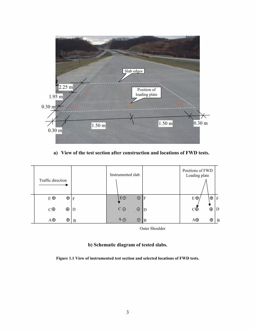
Deflection measurements of rigid pavement slabs were recorded by performing the FWD test on 3 different slabs of an instrumented test section in West Virginia. The tests were conducted using the West Virginia Division of Highways FWD Dynatest device, through a comprehensive program for long term monitoring of newly constructed concrete pavement slabs. For each of the 3 slabs, tests were conducted with an interval of 3 to 4 hours through the 24 hours of the day. FWD test was conducted with a load of 67 KN, and deflection basins were collected from each slab in 6 locations as shown in Figure 1.1. This test was repeated 3 times for different climates. The first was in March 2002, while the second was conducted in June 2002 during daytime only due to difficulties in weather conditions and thunderstorms that prevented testing at night. The test was then repeated in July 2002.
3
a) View of the test section after construction and locations of FWD tests.
b) Schematic diagram of tested slabs.
Figure 1.1 View of instrumented test section and selected locations of FWD tests.
0.30 m 1.50 m 1.50 m 0.30 m
1.95 m
2.25 m
0.30 m
Slab edges
Position of loading plate
Instrumented slabTraffic direction
Outer Shoulder
Positions of FWDLoading plate
B
D
F
A
C
E
B
D
F
A
C
E
B
D
F
A
C
E
4
CHAPTER TWO
FWD TESTING AND RSULTS 2.1 Instrumented Pavement Section
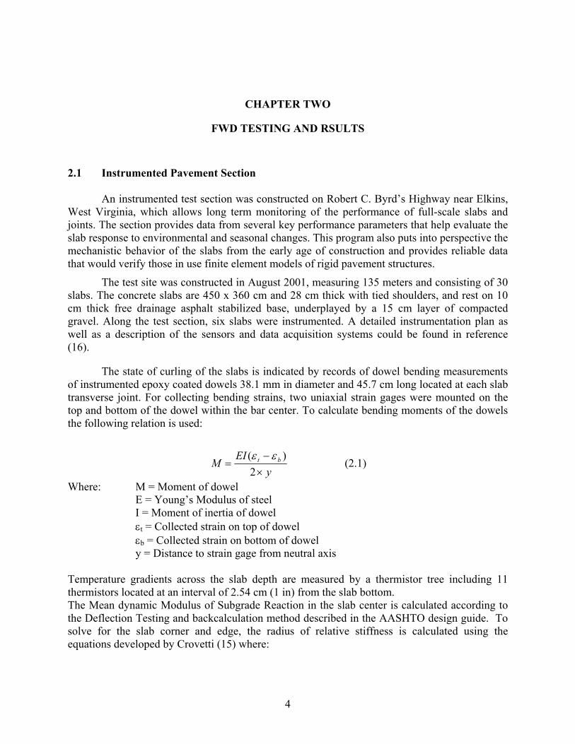
An instrumented test section was constructed on Robert C. Byrd’s Highway near Elkins, West Virginia, which allows long term monitoring of the performance of full-scale slabs and joints. The section provides data from several key performance parameters that help evaluate the slab response to environmental and seasonal changes. This program also puts into perspective the mechanistic behavior of the slabs from the early age of construction and provides reliable data that would verify those in use finite element models of rigid pavement structures.
The test site was constructed in August 2001, measuring 135 meters and consisting of 30 slabs. The concrete slabs are 450 x 360 cm and 28 cm thick with tied shoulders, and rest on 10 cm thick free drainage asphalt stabilized base, underplayed by a 15 cm layer of compacted gravel. Along the test section, six slabs were instrumented. A detailed instrumentation plan as well as a description of the sensors and data acquisition systems could be found in reference (16).
The state of curling of the slabs is indicated by records of dowel bending measurements of instrumented epoxy coated dowels 38.1 mm in diameter and 45.7 cm long located at each slab transverse joint. For collecting bending strains, two uniaxial strain gages were mounted on the top and bottom of the dowel within the bar center. To calculate bending moments of the dowels the following relation is used:
yEI
M bt
×−
=2
)( εε (2.1)
Where: M = Moment of dowel E = Young’s Modulus of steel I = Moment of inertia of dowel εt = Collected strain on top of dowel εb = Collected strain on bottom of dowel y = Distance to strain gage from neutral axis Temperature gradients across the slab depth are measured by a thermistor tree including 11 thermistors located at an interval of 2.54 cm (1 in) from the slab bottom. The Mean dynamic Modulus of Subgrade Reaction in the slab center is calculated according to the Deflection Testing and backcalculation method described in the AASHTO design guide. To solve for the slab corner and edge, the radius of relative stiffness is calculated using the equations developed by Crovetti (15) where:
5
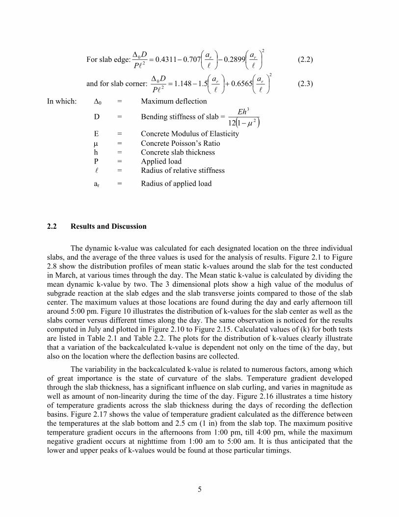
For slab edge:2
20 2899.0707.04311.0
−
−=
∆lll
rr aaP
D (2.2)
and for slab corner: 2
20 6565.05.1148.1
+
−=
∆lll
rr aaP
D (2.3)
In which: ∆0 = Maximum deflection
D = Bending stiffness of slab = ( )2
3
112 µ−Eh
E = Concrete Modulus of Elasticity µ = Concrete Poisson’s Ratio h = Concrete slab thickness P = Applied load l = Radius of relative stiffness
ar = Radius of applied load
2.2 Results and Discussion
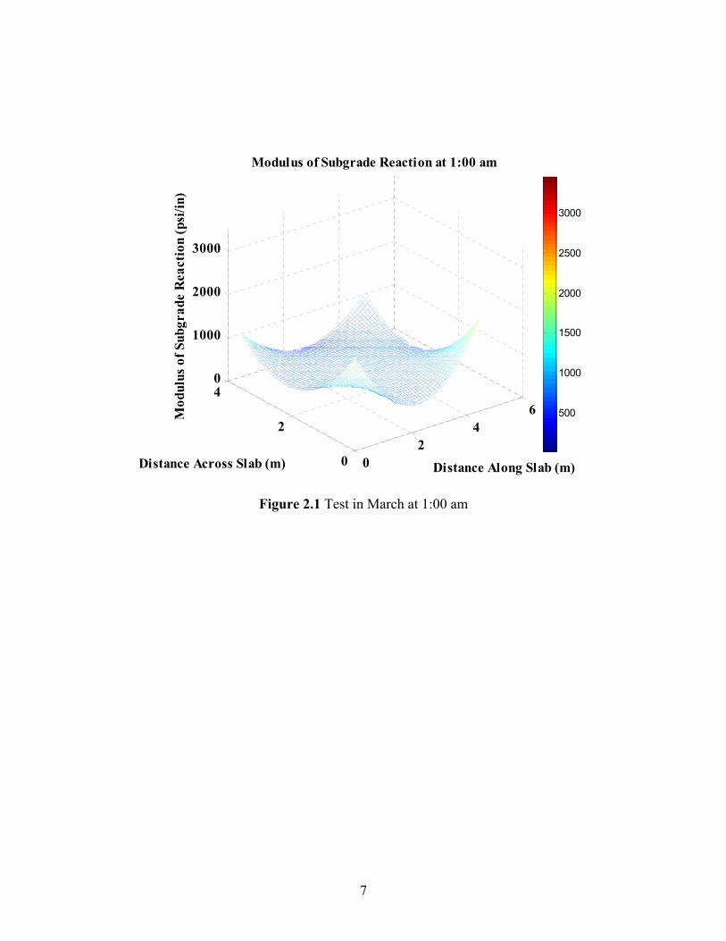
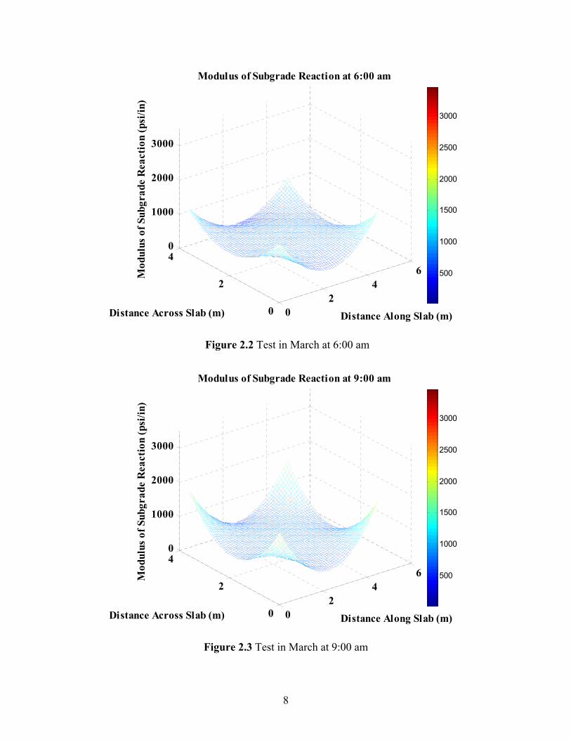
The dynamic k-value was calculated for each designated location on the three individual
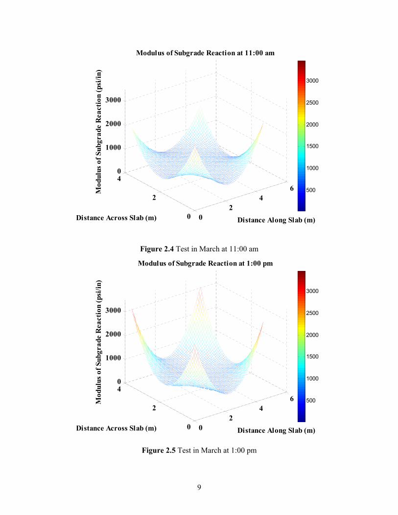
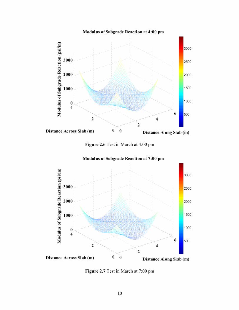
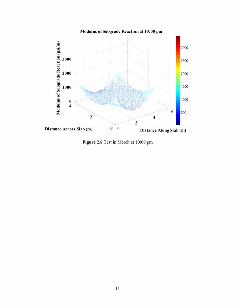
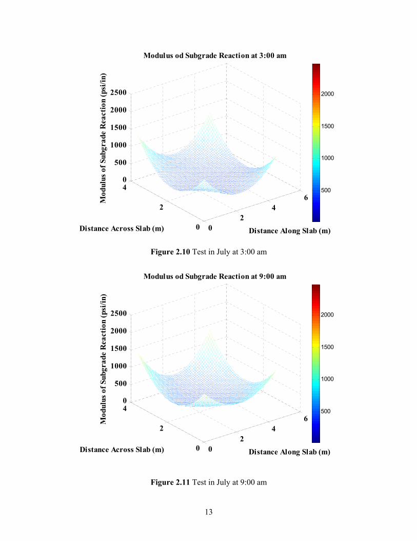
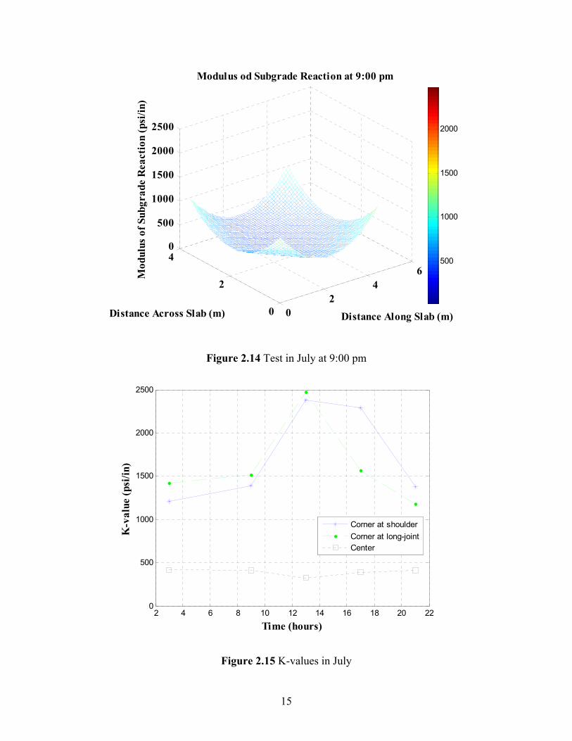
slabs, and the average of the three values is used for the analysis of results. Figure 2.1 to Figure 2.8 show the distribution profiles of mean static k-values around the slab for the test conducted in March, at various times through the day. The Mean static k-value is calculated by dividing the mean dynamic k-value by two. The 3 dimensional plots show a high value of the modulus of subgrade reaction at the slab edges and the slab transverse joints compared to those of the slab center. The maximum values at those locations are found during the day and early afternoon till around 5:00 pm. Figure 10 illustrates the distribution of k-values for the slab center as well as the slabs corner versus different times along the day. The same observation is noticed for the results computed in July and plotted in Figure 2.10 to Figure 2.15. Calculated values of (k) for both tests are listed in Table 2.1 and Table 2.2. The plots for the distribution of k-values clearly illustrate that a variation of the backcalculated k-value is dependent not only on the time of the day, but also on the location where the deflection basins are collected.
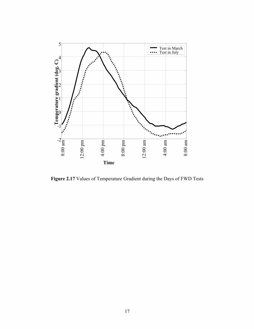
The variability in the backcalculated k-value is related to numerous factors, among which of great importance is the state of curvature of the slabs. Temperature gradient developed through the slab thickness, has a significant influence on slab curling, and varies in magnitude as well as amount of non-linearity during the time of the day. Figure 2.16 illustrates a time history of temperature gradients across the slab thickness during the days of recording the deflection basins. Figure 2.17 shows the value of temperature gradient calculated as the difference between the temperatures at the slab bottom and 2.5 cm (1 in) from the slab top. The maximum positive temperature gradient occurs in the afternoons from 1:00 pm, till 4:00 pm, while the maximum negative gradient occurs at nighttime from 1:00 am to 5:00 am. It is thus anticipated that the lower and upper peaks of k-values would be found at those particular timings.
6
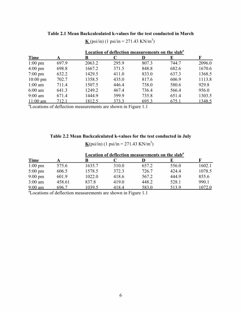
Table 2.1 Mean Backcalculated k-values for the test conducted in March K (psi/in) (1 psi/in = 271.43 KN/m3)
Location of deflection measurements on the slaba
Time A B C D E F 1:00 pm 697.9 2063.2 295.9 807.3 744.7 2096.0 4:00 pm 698.8 1667.2 371.5 848.8 682.6 1670.6 7:00 pm 632.2 1429.5 411.0 833.0 637.3 1368.5 10:00 pm 702.7 1358.5 435.0 817.6 606.9 1113.8 1:00 am 711.4 1507.5 446.4 738.0 580.6 929.8 6:00 am 641.3 1249.2 467.4 736.4 566.4 956.0 9:00 am 671.4 1444.9 399.9 735.8 651.4 1303.5 11:00 am 712.1 1812.5 373.3 695.3 675.1 1348.5 aLocations of deflection measurements are shown in Figure 1.1
Table 2.2 Mean Backcalculated k-values for the test conducted in July K(psi/in) (1 psi/in = 271.43 KN/m3)
Location of deflection measurements on the slaba
Time A B C D E F 1:00 pm 575.6 1635.7 310.0 657.2 556.0 1602.1 5:00 pm 606.5 1578.5 372.3 726.7 424.4 1078.5 9:00 pm 601.9 1022.0 418.6 567.2 444.9 855.6 3:00 am 458.61 837.8 419.0 448.2 528.1 990.1 9:00 am 696.7 1039.5 418.4 583.0 513.9 1072.0 aLocations of deflection measurements are shown in Figure 1.1
7
02
46
0
2
40
1000
2000
3000
Distance Along Slab (m)
Modulus of Subgrade Reaction at 1:00 am
Distance Across Slab (m)
Mod
ulus
of S
ubgr
ade
Rea
ctio
n (p
si/in
)
500
1000
1500
2000
2500
3000
Figure 2.1 Test in March at 1:00 am
8
02
46
0
2
40
1000
2000
3000
Distance Along Slab (m)
Modulus of Subgrade Reaction at 6:00 am
Distance Across Slab (m)
Mod
ulus
of S
ubgr
ade
Rea
ctio
n (p
si/in
)
500
1000
1500
2000
2500
3000
Figure 2.2 Test in March at 6:00 am
02
46
0
2
40
1000
2000
3000
Distance Along Slab (m)
Modulus of Subgrade Reaction at 9:00 am
Distance Across Slab (m)
Mod
ulus
of S
ubgr
ade
Rea
ctio
n (p
si/in
)
500
1000
1500
2000
2500
3000
Figure 2.3 Test in March at 9:00 am
9
02
46
0
2
40
1000
2000
3000
Distance Along Slab (m)
Modulus of Subgrade Reaction at 11:00 am
Distance Across Slab (m)
Mod
ulus
of S
ubgr
ade
Rea
ctio
n (p
si/in
)
500
1000
1500
2000
2500
3000
Figure 2.4 Test in March at 11:00 am
02
46
0
2
40
1000
2000
3000
Distance Along Slab (m)
Modulus of Subgrade Reaction at 1:00 pm
Distance Across Slab (m)
Mod
ulus
of S
ubgr
ade
Rea
ctio
n (p
si/in
)
500
1000
1500
2000
2500
3000
Figure 2.5 Test in March at 1:00 pm
10
02
46
0
2
40
1000
2000
3000
Distance Along Slab (m)
Modulus of Subgrade Reaction at 4:00 pm
Distance Across Slab (m)
Mod
ulus
of S
ubgr
ade
Rea
ctio
n (p
si/in
)
500
1000
1500
2000
2500
3000
Figure 2.6 Test in March at 4:00 pm
02
46
0
2
40
1000
2000
3000
Distance Along Slab (m)
Modulus of Subgrade Reaction at 7:00 pm
Distance Across Slab (m)
Mod
ulus
of S
ubgr
ade
Rea
ctio
n (p
si/in
)
500
1000
1500
2000
2500
3000
Figure 2.7 Test in March at 7:00 pm
11
02
46
0
2
40
1000
2000
3000
Distance Along Slab (m)
Modulus of Subgrade Reaction at 10:00 pm
Distance Across Slab (m)
Mod
ulus
of S
ubgr
ade
Rea
ctio
n (p
si/in
)
500
1000
1500
2000
2500
3000
Figure 2.8 Test in March at 10:00 pm
12
0 5 10 15 20 25500
1000
1500
2000
2500
3000
3500
Time (hours)
K-v
alue
(psi
/in)
Corner at shoulderCorner at long-jointCenter
Figure 2.9 K-values in March
13
02
46
0
2
40
500
1000
1500
2000
2500
Distance Along Slab (m)
Modulus od Subgrade Reaction at 3:00 am
Distance Across Slab (m)
Mod
ulus
of S
ubgr
ade
Rea
ctio
n (p
si/in
)
500
1000
1500
2000
Figure 2.10 Test in July at 3:00 am
02
46
0
2
40
500
1000
1500
2000
2500
Distance Along Slab (m)
Modulus od Subgrade Reaction at 9:00 am
Distance Across Slab (m)
Mod
ulus
of S
ubgr
ade
Rea
ctio
n (p
si/in
)
500
1000
1500
2000
Figure 2.11 Test in July at 9:00 am
14
02
46
0
2
40
500
1000
1500
2000
2500
Distance Along Slab (m)
Modulus od Subgrade Reaction at 1:00 pm
Distance Across Slab (m)
Mod
ulus
of S
ubgr
ade
Rea
ctio
n (p
si/in
)
500
1000
1500
2000
Figure 2.12 Test in July at 1:00 am
02
46
0
2
40
500
1000
1500
2000
2500
Distance Along Slab (m)
Modulus od Subgrade Reaction at 5:00 pm
Distance Across Slab (m)
Mod
ulus
of S
ubgr
ade
Rea
ctio
n (p
si/in
)
500
1000
1500
2000
Figure 2.13 Test in July at 5:00 pm
15
02
46
0
2
40
500
1000
1500
2000
2500
Distance Along Slab (m)
Modulus od Subgrade Reaction at 9:00 pm
Distance Across Slab (m)
Mod
ulus
of S
ubgr
ade
Rea
ctio
n (p
si/in
)
500
1000
1500
2000
Figure 2.14 Test in July at 9:00 pm
2 4 6 8 10 12 14 16 18 20 220
500
1000
1500
2000
2500
Time (hours)
K-v
alue
(psi
/in)
Corner at shoulderCorner at long-jointCenter
Figure 2.15 K-values in July
16
a) Temperature gradient across slab cross section in March
b) Temperature gradient across slab cross section in July
Figure 2.16 Temperature Gradient Profiles During the Days of FWD Testing
Figure 2.17 Values of Temperature Gradient during the Days of FWD Tests
8:00
am-2
-1
0
1
2
3
4
5
Time
Tem
pera
ture
gra
dien
t (de
g. C
)
Test in MarchTest in July
12:0
0 pm
4:00
pm
8:00
pm
12:0
0 am
4:00
am
8:00
am
18
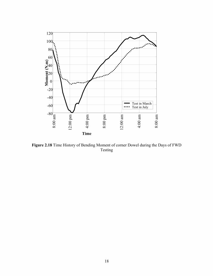
Figure 2.18 Time History of Bending Moment of corner Dowel during the Days of FWD Testing
-80
-60
-40
-20
0
20
40
60
80
100
120
Mom
ent (
N.m
)
Test in MarchTest in July
8:00
am
Time
12:0
0 pm
4:00
pm
8:00
pm
12:0
0 am
4:00
am
8:00
am
19
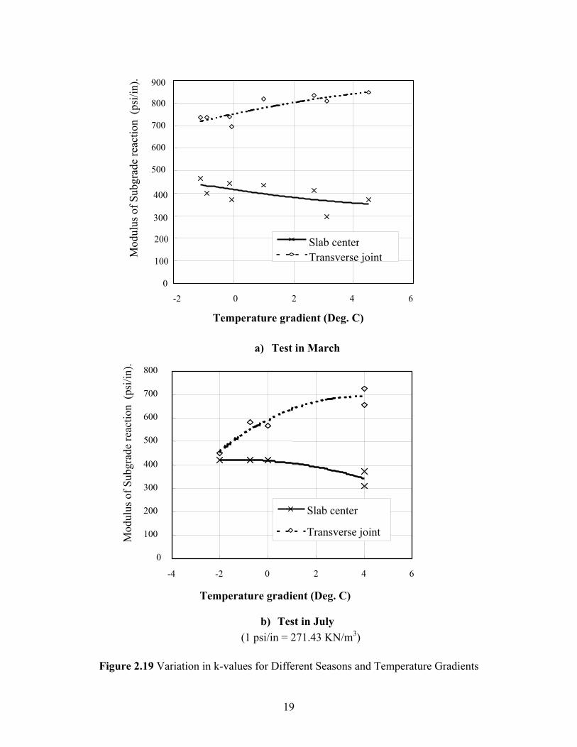
a) Test in March
b) Test in July
Figure 2.19 Variation in k-values for Different Seasons and Temperature Gradients
Mod
ulus
of S
ubgr
ade
reac
tion
(psi
/in).
0
100
200
300
400
500
600
700
800
-4 -2 0 2 4 6
Temperature gradient (Deg. C)
Slab center
Transverse joint
0
100
200
300
400
500
600
700
800
900
-2 0 2 4 6
Temperature gradient (Deg. C)
Mod
ulus
of S
ubgr
ade
reac
tion
(psi
/in).
Slab centerTransverse joint
(1 psi/in = 271.43 KN/m3)
20
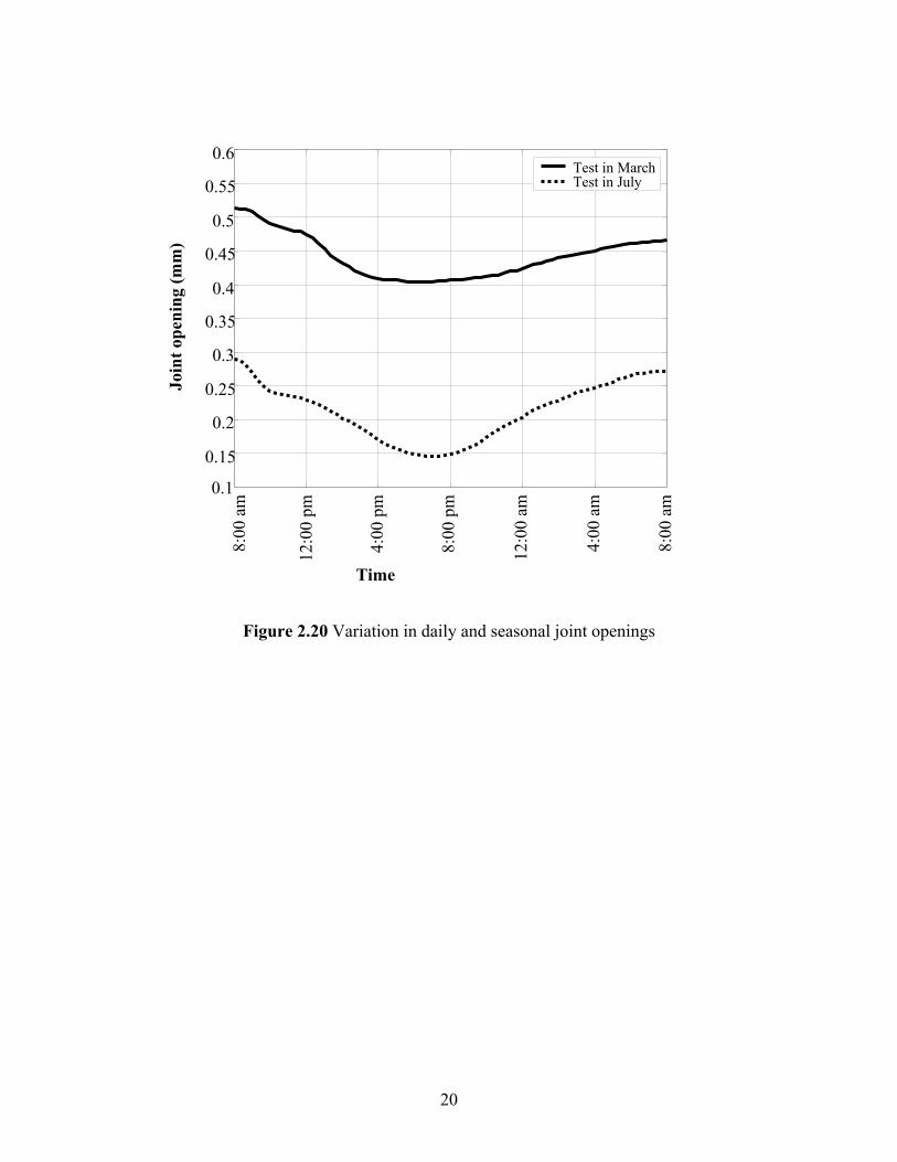
Figure 2.20 Variation in daily and seasonal joint openings
0.1
0.15
0.2
0.25
0.3
0.35
0.4
0.45
0.5
0.55
0.6 Test in MarchTest in July
8:00
am
12:0
0 pm
4:00
pm
8:00
pm
12:0
0 am
4:00
am
8:00
am
Join
t ope
ning
(mm
)
Time
21
Seasonal change in ambient temperature alters the overall temperature of the slab, resulting in different amounts of expansion and contraction. The recorded temperature of the tested slabs varied from March to July from 10oC to 29.5oC. Seasonal changes also include variability in precipitation levels, frost depths, degree of saturation and movement of water table. Slab curvature could also result of built in construction curling of the slabs due to the combined effect of drying shrinkage of the concrete material and the formation of a high positive temperature gradient after placement (17, 18). The variation of backcalculated k-value could be explained insight of the slab deformation when subjected to temperature variations as follows:
In the case of a positive temperature gradient across the slab thickness, the longitudinal slab edges and transverse joints tend to curl downwards and the maximum deflection occurs at the slab corners. This behavior compels the under laying strata to compress at those locations where the maximum contact area between the slab base and the base layer takes place. Under this action, if the slab weight is not large enough to bring the slab center into contact with the base layer, a gap occurs at this location. This is observed by the high magnitude of k-value backcalculated at the slab edges and corners relative to those of the slab center. On the other hand, when the slab is subjected to a negative temperature gradient, the slab edges tend to curl upward against gravity restoring its original position, and the largest contact area between the slab bottom and the base layer occurs at the slab center, increasing the k-value at this location.
This behavior is well identified in Figure 2.9 and Figure 2.15 where the largest k-values occur at the slab corners around 4:00 pm to 5:00 pm while minimum k-values are noticed at the slab center. During this time period the slab is subjected to maximum positive temp gradient.
The largest deformation of the slab will occur at the slab edges and is demonstrated through measurements of the corner dowel bending moments as shown in Figure 19. The change in dowel bending moments follows the change in the temperature gradient along the hours of the day, indicating the dominant effect of this temperature gradient on the slab deformation. The values of the dowel bending moments are in good agreement with those recorded by Sargand (19), in the experimental section in Ohio.
For the purpose of comparing the k-values according to the location of the FWD test, the values calculated at the transverse joint, as well as in the slab center will be considered. Results at corners show significantly high values while those k-values at the slab edges near the shoulder and at the longitudinal joint show more significant variability in magnitude during different hours of the day. The variation in backcalculated modulus of subgrade reaction is plotted against variation in temperature gradients in Figure 20. For the case of the slab center, the k-value is indirectly proportional to the values of temperature gradients, and vice versa for the case at the transverse joints. This observation confirms the concept of slab deformation and contact area between the slab and the base under the effect of temperature gradients. In July, the overall temperature of the slab is three times higher than that in March. It is anticipated that the deformation of the slab will be larger, and this is reflected on the larger variation of (k) calculated at the transverse joint in comparison with those calculated in March.
Considering the test conducted in July, it is noticed that (k) approaches the same value at both positions of the transverse joint and the slab center at the time when maximum negative
22
gradient occurs. This observation indicates that at the maximum negative gradient the slab was able to restore the same contact characteristics between its base and the underlying strata along its length. This concept could also be noticed in Figure 2.18, where the magnitude of dowel bending didn’t change from positive to negative as the case in the month of March. Furthermore, Figure 2.20 illustrates the variation of joint openings between the month of March and July during the days of testing. The higher values of the joint opening in March indicate that the slabs are in a state of contraction compared to that in July, thus greater contact areas and compaction of the base layer take place, resulting in higher values of (k).
Statistical analysis of the calculated k-values show that the standard deviation of the results calculated at the slab center are far smaller that those calculated for the results obtained at the slab corners. For the test conducted in July the standard deviation for the slab corner near the shoulder and near the longitudinal joint amounts 557 and 493 respectively. While that for the slab center was calculated to be 39. Similarly those calculated for the test in March are 499 at the shoulder corner, 666 for the long-joint corner and 76 at the slab center. This clearly illustrates that the variability of K-values at the slab center is smaller compared to those at other locations of the slab.
23
CHAPTER THREE
CONCLUSIONS This study is based on field data and FWD tests performed on a newly constructed rigid pavement section in West Virginia. According to the results presented in this investigation, the Modulus of subgrade reaction backcalculated from deflection basins is sensitive to the temperature gradients across the slab thickness, and consequently to the position where those deflection basins are recorded. Observation of the backcalculated k-values at the slab center demonstrated that during springtime, (k) varies according to the time of the day up to 17 %. Similar variation was also recorded in Summer time at the slab center, while the variation in transverse joints where up to 50 % along the day. The presented results are attributed to the structural and environmental characteristics of the newly constructed instrumented test section in West Virginia, while the degree of variability in k-value may vary according to the effect of several pavement variables including the slab thickness, type of base, degree of saturation, efficiency of dowel bar support at transverse joints and moisture variation across the slab thickness.
The AASHTO design guide describes a procedure to account for seasonal changes while calculating the mean design modulus of subgrade reaction. Observation of the backcalculated k-values indicate that selecting the timing and position of performing the FWD test for the purpose of collecting deflection basins in each season are significant to minimize errors. The slab center showed the least variation in backcalculated k-values compared to slab edges and corners. It was also demonstrated that backcalculated k-values tend to approach close values for those at the transverse joint and at the slab center at time of negative temperature gradient across the slab thickness. Therefore it is recommended to record deflection basins for backcalculations either in late evening or in early morning.
24
REFERENCES 1. Westergaard, H.M. Computation of stresses in Concrete Roads. Proceedings, Highway
Research Board, 1925. 2. Hall, K.T., Performance, Evaluation, and Rehabilitation of Asphalt-overlaid Concrete
Pavements. Ph.D. thesis, University of Illinois at Urbana-Champaign, 1991. 3. Hall, K.T. Backcalculation Solutions for Concrete Pavement. Technical memo prepared for
SHRP Contract O-020, Long-term Pavement Performance Data Analysis, 1992. 4. Supplement to the AASHTO Guide for Design of Pavement Structures, Part II, - Rigid
Pavement Design & Rigid Pavement Joint Design, American Association of State Highway and Transportation Officials, ISBN 1-56051-078-1, 1998.
5. Darter M.I., K. Hall, and C. Kuo. Support Under Concrete Pavements. National Cooperative Highway Research Program, Transportation Research Board, National Research Council, 1994.
6. Westergaard H.M. Analysis of stresses in concrete pavements due to variations of temperature. Proceeding, 6th Annual Meeting, highway Research Board, 1926, pp. 201-217.
7. Tang T., D.G. Zoolinger, and S. Senadheera. Analysis of Concave Curling in Concrete Slabs. Journal of Transportation Engineering, Vol. 119, No. 4, 1993, pp. 618-633.
8. Teller L.W. and E.C. Sutherland. The Structural Design of Concrete Pavements, Part 2: Observed Effects of Variations in Temperature and Moisture on the Size, Shape, and Stress Resistance of Concrete Pavement Slabs. Public Roads, Vol. 16, No. 9, 1935, pp. 169-197.
9. Hveem F.N. A report of an Investigation to Determine Causes for Displacement and Faulting at the Joints in Portland Cement Concrete Pavements. State of California Report, Division of Highways, Material and Research Department, 1949.
10. Yu H.T., L. Khazanovich, M. I. Darter, and A. Ardani. Analysis of Concrete Pavement Responses to Temperature and Wheel Loads Measured from Instrumented Slabs. Proc. 77th Annual Meeting, Transportation Research Board, Washington DC, 1998.
11. Shoukry S.N. Backcalculation of Thermally Deformed Concrete Pavements. Proc. 79th Annual Meeting, Transportation Research Board, 2000.
12. William G., and S. Shoukry. 3D Finite Element Analysis of Temperature-Induced Stresses in Dowel Jointed Concrete Pavements. The In international Journal of Geomechanics, Vol. 1, No. 3, 2001, pp. 291-307, 2001.
13. Ioannides, A.M. Dimensional Analysis of NDT Rigid Pavement Evaluation. Journal of Transportation Engineering, Vol. 116, No. 1, 1990, pp. 23-26.
14. Ioannides, A.M. Concrete Pavement Backcalculation using ILLI-Back 3.0. Nondestructive Testing of Pavements and Backcalculation of Moduli (Second Volume), STP 1198, American Society for Testing and Materials, Philadelphia, PA, 1994, pp. 103-124.
15. Crovetti J.A. Evaluation of Jointed Concrete Pavement Systems Incorporating Open-Graded Permeable Bases. Ph.D. thesis, University of Illinois at Urbana-Champaign, 1994.
16. Shoukry, S.N. West Virginia Instrumented Concrete Pavement: Curing and Temperature Induced Strains During the First 90 Days. Data analysis Work Group, 81st Annual Transportation Research Board Meeting, Washington D.C., January 2002.
17. Eisnmann J., and G. Leykauf. Effect of Paving Temperatures on Pavement Performance. Proceedings of the Second International Workshop on the Design and the Evaluation of Concrete Pavements, Siguenza, Spain, 1990.
25
18. Franklin R.E. Effect of Weather Conditions on Early Strains in Concrete Slabs. RRL Report No. LR266, Road Research Laboratory, Crowthrone, Berkshire, UK, 1969.
19. Sargand S.M. Performance of Dowel Bars and Rigid Pavement. Draft Final Report, Ohio University, Ohio Research Institute for Transportation and The Environment, Athens, Ohio, 2000.