Effect of Halite (NaCl) on Sandstone permeability and well ...usir.salford.ac.uk/44572/3/PhD Final...

Effect of Halite (NaCl) on Sandstone permeability and well

injectivity during CO2 storage in Saline Aquifers

Ramadan Makhzoom Benashor

(B.Sc. Eng., M.Sc.)

School of Computing Science and Engineering

Petroleum Technology and Spray Research Groups

University of Salford

Manchester, UK

Submitted in Partial Fulfilment of the Requirements of the Degree of Doctor of

Philosophy, September 2017

i

Abstract

Carbon dioxide capture and storage (CCS) is one of the widely discussed options for

decreasing CO2 emissions. This method requires the techniques for capturing purification of

anthropogenic CO2 from fossil-fuel power plants, subsequent compression and transport, and,

ultimately, its storage in deep geological formations. Due to the high formation salinity, there

is a substantial concern about the near well bore formation dry out as a result salt

precipitation in the form of halite (NaCl). The focus was on one of the important physical

mechanisms of CO2 injection into deep saline aquifers. The salt (mainly halite) will

eventually fully saturate the brine causing the salt to start precipitating as solids. This solid

precipitation could significantly decrease the porosity and permeability of the porous

medium.

The investigations, in this study, were carried out in three distinct parts: (i) core flooding tests

for different sandstone core samples (Bentheimer, Castlegate and Idaho Gray) which were

saturated with different brine concentrations to measure the CO2 flow rate for different

injection pressures, (ii) utilising simulated experimental apparatus to estimate the porosity

and permeability of the core samples and (iii) Qualitative analysis of porosities using CT

scanner.

In Part (i), it was found that the CO2 flow rates vary from 0.4 to 6.0 l/min when using brine

solution concentrations of 10, 15, 20 and 26.4% for core flooding tests of the studied

sandstone core samples before diluting concentrations with sea water (3.5%), and after

diluting by sea water the flow rates vary from 0.6 to 7.0 l/min. The flow rate increase

indicates that the injectivity will increase.

In part (ii), Helium Gas Porosimeter was used to calculate the porosity of each core sample

and the results showed for Bentheimer, Castlegate and Idaho Gray 20.8 %, 25.6 % and 23.4

% respectively. Liquid saturating method was also used to calculate the porosity of each core

sample and the results showed 23.6% for Bentheimer, 24.4% for Castlegate and 22.4% for

Idaho Gray. Regarding the permeability impairment investigations for both brine

permeability and gas permeability, the permeability damage took place due to the salt

precipitation (NaCl) phenomenon. For brine permeability, the damage percentage of

Bentheimer, Castlegate and Idaho Gray was 40%, 42% and 47%. For gas permeability the

reduction due to dry out of saturated samples with 20% brine solution were calculated as

34.5% for Bentheimer, 42% for Castlegate and 50.2% for Idaho Gray.

Finally, in part (iii), CT Scann was used to determine each core sample porosity and the

results showed 20.7% for Bentheimer, 24.3% for Castlegate and 24.6% for Idaho Gray

ii

Acknowledgements

I would like to express my gratitude and sincere thanks to Dr Amir Norian and Prof G.G.

Nasr for their helpful advice, endless support and help throughout the course of this work.

Their guidance has been fruitful in steering the direction of this project.

My wife was my greatest support during the last few years. Her loyalty, faithfulness, patience

and positive enthusiasm provided the much-needed strength during the preparation of this

thesis. I am extremely grateful for everything she did including spending much of her time

taking care of our lovely children Abedalbadie, Reham and Fatima so to allow me the time

for my research. My acknowledgement goes to the scholarship from Libyan High Educational

studies through the cultural section of Libyan embassy in London, Uk.

In addition, I would like to thank all the staff members and my colleagues at the Petroleum

and Gas Engineering department, particularly Dr Enyi Godpower, Dr A.J. Abbas, Mr Aminu

Abba Yahaya and Mr Alan Mapin for their valuable and constant support.

iii

Declaration

I, Ramadan Makhzoom Benashor, declare that this dissertation report is my original work,

and has not been defer to elsewhere for any award. Any section, part or phrasing that has

been used or copied from other literature or documents copied has been clearly referenced at

the point of use as well as in the reference section of the thesis work.

________________ _______________

Signature Date / /

________________ ________________

Approved by

iv

Dedication

This work is dedicated to

My remarkable wife, Nesren Flah

And

My smart children

Abedalbadie, Reham and Fatima

And my wonderful mother, Fatima Ali

v

List of Publications

1- Benashor, R. M. Z., Nourian, A., Nasr, G., & Enyi, G. C. (2016). The Effects of

Dissolved Sodium Chloride (NaCl) on Well Injectivity during CO 2 Storage into

Saline Aquifers, 6 (2), 11–22.

2- Benashor, R. M. Z., Nourian, A., Nasr, G., & Abbas, A. J. (2016). Well Injectivity

Management during Geological Carbon Sequestration Activity, 6(2), 11–22.

3- R .M. Benashor, A. Nourian and G G Nasr, University of Salford, UK. Experimental

investigations to study the effects of halite (NaCl) precipitation on sandstone

permeability and injectivity during CO2 storage into saline aquifers. 6th International

Conference on Petroleum Engineering ,June 29-30, 2017 ,Madrid, Spain

vi

List of symbols and abbreviations

CCS Carbon dioxide capture and storage

GHG Greenhouse gases

IPCC Intergovernmental panel on climate change

IEA International energy agency

CO2 Carbon dioxide

PPM part per million

Ppg Ib/gallon

Gt Giga ton

Mt Mega ton

EOR Enhanced Oil Recovery

MPa Mega Pascale

mD Milli Darcy

CAB CO2 alternating brine

CBM coal bed methane

Mt mega tonnes

t/day ton /day

Mt/yr mega tonne per year

NaCl Sodium chloride

H2S Hydrogen sulphide

ROI Region of interest

CT Computed Topography

NOX Nitrous oxide

CH4 Methane

Vp Pore volume of the core sample

Vb Bulk volume of the core sample

Vg Grain volume of the core sample

K Rock permeability

Rock porosity

vii

Conversion Table

1 D 1000 millidarcy

1 ton one metric ton = 1000 kg

1 mt one mega ton = 10 6 ton

1 Gt one gaga ton = 1000 mt = 10 9 ton

1 atm 14.6959 psi

1 atm 101325.01 Pascal

1 atm 1.0132501 bar

1 bar 14.50377 psi

Poise 100 cp

1 m 100 cm

1 ft 30.48 cm

1 inch 2.54 cm

viii

ix

Table of Contents

Abstract ................................................................................................................................................... i

Acknowledgements ............................................................................................................................... ii

Declaration ........................................................................................................................................... iii

Dedication ............................................................................................................................................. iv

List of Publications ............................................................................................................................... v

List of symbols and abbreviations ...................................................................................................... vi

Table of Contents ................................................................................................................................ ix

List of Figures ..................................................................................................................................... xiii

List of Tables ...................................................................................................................................... xvi

Chapter 1: Introduction ....................................................................................................................... 1

1.1. Risks associated with CO2 underground storage ............................................................................. 3

1.3. Overall Aim ..................................................................................................................................... 4

1.4. Objectives ........................................................................................................................................ 4

1.5. Thesis structure ................................................................................................................................ 4

Chapter 2: Literature Review .............................................................................................................. 6

2.1 Overview ................................................................................................................................. 6

2.2 Sources of CO2 ........................................................................................................................ 7

2.3 Global Warming and CO2 Emissions ...................................................................................... 7

2.4 CO2 Storage Options ............................................................................................................... 9

2.5 CO2 Storage into Saline Aquifer ............................................................................................. 9

2.5.1 Why Saline Aquifers ..................................................................................................... 10

2.5.2 Reservoir Properties of Saline Aquifers ........................................................................ 11

2.6 Trapping Mechanism ............................................................................................................ 12

2.7 CO2 Injection Approaches .................................................................................................... 13

2.8 Present and Scheduled CO2 Projects ..................................................................................... 13

x

2.9 Risks Posed by CO2 Geological Storage ............................................................................... 13

2.9.1 Salt Precipitation and Dry out in the near- Wellbore .................................................... 14

2.10 Approaches to Restore the Well Injectivity .......................................................................... 16

2.10.1 Fracture managements .................................................................................................. 17

2.10.2 Perforation ..................................................................................................................... 17

2.10.3 Acid management ......................................................................................................... 18

2.11 Optimisation of CCS Costs ................................................................................................... 18

2.12 Rock properties ..................................................................................................................... 19

2.13 Classification of Porosity ...................................................................................................... 19

2.13.1 Effective Porosity .......................................................................................................... 20

2.13.2 Absolute Porosity .......................................................................................................... 20

2.14 Permeability .......................................................................................................................... 21

2.15 Saturation .............................................................................................................................. 22

2.16 Well Injectivity ..................................................................................................................... 22

2.17 CT scan ................................................................................................................................. 24

2.18 Summary ............................................................................................................................... 25

Chapter 3: Experiment Apparatus and Methodology of Data Processing .................................... 26

3.1.1 Salinity Measurement ................................................................................................... 30

3.1.2 Viscosity Measurement ................................................................................................. 31

3.1.3 Density .......................................................................................................................... 33

3.1.4. Errors and Accuracy ............................................................................................................... 35

3.2 PHASE-I: Core Flooding Tests ............................................................................................ 35

3.2.1 Experimental set up ....................................................................................................... 37

3.2.2 Methodology of measurement ...................................................................................... 39

3.2.3 Errors and Accuracy...................................................................................................... 41

3.3 Phase-II: Porosity and Permeability ...................................................................................... 41

xi

3.3.1 Description of Apparatus .............................................................................................. 41

3.3.2 Methodology of Measurement ...................................................................................... 44

Measurement of Bulk Volume ...................................................................................................... 46

Measurement of Pore Volume ...................................................................................................... 46

Measurement of Grain Volume..................................................................................................... 46

3.4 PHASE-III: CT scan ............................................................................................................. 57

3.4.1 Equipment description and principles of X-Ray inspection ......................................... 57

3.4.2 Methodology of measurement ...................................................................................... 60

3.4.3 Errors and Accuracy...................................................................................................... 66

3.5 Chapter Summary ................................................................................................................. 67

Chapter 4: Results and Discussion .................................................................................................... 68

4.1 Sample preparation ............................................................................................................... 68

4.1.1 Salinity .......................................................................................................................... 69

4.1.2 Viscosity ....................................................................................................................... 69

4.1.3 Density .......................................................................................................................... 69

4.1.4 Density, Viscosity and Salinity relationships................................................................ 70

4.2 PHASE – I Core flooding tests ............................................................................................. 72

4.2.1 Core flooding tests for Bentheimer sandstone .............................................................. 72

4.2.2 Core flooding tests for Castlegate sandstone ................................................................ 78

4.2.3 Core flooding tests for Idaho gray sandstone ................................................................ 83

4.3 PHASE-II Porosity & Permeability ...................................................................................... 89

4.3.1 Porosity ......................................................................................................................... 89

4.3.2 Permeability .................................................................................................................. 93

4.3.3 Effect of Salinity on liquid Permeability ...................................................................... 94

4.3.4 Effect of Salinity on gas Permeability .......................................................................... 98

4.4 The Porosity and the Brine Permeability Relationship ....................................................... 103

xii

4.4.1 The Porosity and the Brine Permeability Relationship ............................................... 104

4.4.2 The Porosity and the gas Permeability Relationship ................................................... 105

4.5 PHASE III: CT scanning .................................................................................................... 106

4.5.1 CT scan of Bentheimer sandstone ............................................................................... 106

4.5.2 CT scan of Castlegate sandstone ................................................................................. 106

4.5.3 CT scan of Idaho gray sandstone ................................................................................ 108

4.5.4 Images and visualisation of the scanned core sample ................................................. 109

4.5.5 CT Scan Visualisation and Quantification of Salt Precipitation ................................. 111

4.5.6 Porosity determination summary ................................................................................ 112

4.6 Summary ............................................................................................................................. 113

Chapter 5: Conclusion and Recommendations .............................................................................. 115

5.1 Conclusions ......................................................................................................................... 115

5.2 Future work and recommendation ...................................................................................... 116

References .......................................................................................................................................... 117

APPENDIX – A: Journal Publications ........................................................................................... 120

xiii

List of Figures

Figure 2.1 : The CCS process ................................................................................................................. 7

Figure 2.2 : Origin of anthropogenic CO2 emissions .............................................................................. 8

Figure 2.3 : Options for CO2 storage in deep geological underground formations [1] ........................... 9

Figure 2.4 : Trapping mechanisms for CO2 storing in deep saline aquifers A) structural trapping, B)

capillary trapping, C) dissolution and D) mineral trapping .................................................................. 12

Figure 2.5 : Schematic of CO2/water mutual dissolution in porous media [39] ................................... 15

Figure 2.6 : Pressure and time relationship under various CO2 injection rates ..................................... 17

Figure 2.7 : the scheme of cost optimisation of CCS[30] ..................................................................... 18

Figure 2.8 : (a) Cubical packing, (b) rhombohedra, (c) cubical packing with two grain sizes, and (d)

typical sand with irregular grain shape ................................................................................................. 19

Figure 2.9 : Permeability is an indication of how easy it is for the fluids to flow through the medium

[47] ........................................................................................................................................................ 22

Figure 3.1: thesis work plan .................................................................................................................. 27

Figure 3.2: Different Types of Sandstones (a) Bentheimer, (b) Castlegate and (c) Idaho Gray ........... 29

Figure 3.3: Brine solutions in (wt %) .................................................................................................... 30

Figure 3.4 : Refractometer gives the salinity in (wt %) ........................................................................ 31

Figure 3.5 : Electronic Rotational Viscometer ...................................................................................... 32

Figure 3.6 : Mud Balance scale device ................................................................................................. 34

Figure 3.7 : the experimental set up diagram ........................................................................................ 37

Figure 3.8 : Experimental set up ........................................................................................................... 38

Figure 3.9 : Shows the fancher core holder (1”x1”) ............................................................................. 39

Figure 3.10 : PORG – 200 .................................................................................................................... 42

Figure 3.11 : PERL – 200 ..................................................................................................................... 43

Figure 3.12 : PERG – 200 ..................................................................................................................... 44

Figure 3.13: Definition of Darcy's law ................................................................................................. 52

Figure 3.14 : Microfocus – nanofocus .................................................................................................. 58

Figure 3.15 : CT scanner at Salford University .................................................................................... 59

Figure 3.16 : Histogram and scan optimiser for Bentheimer sandstone ............................................... 61

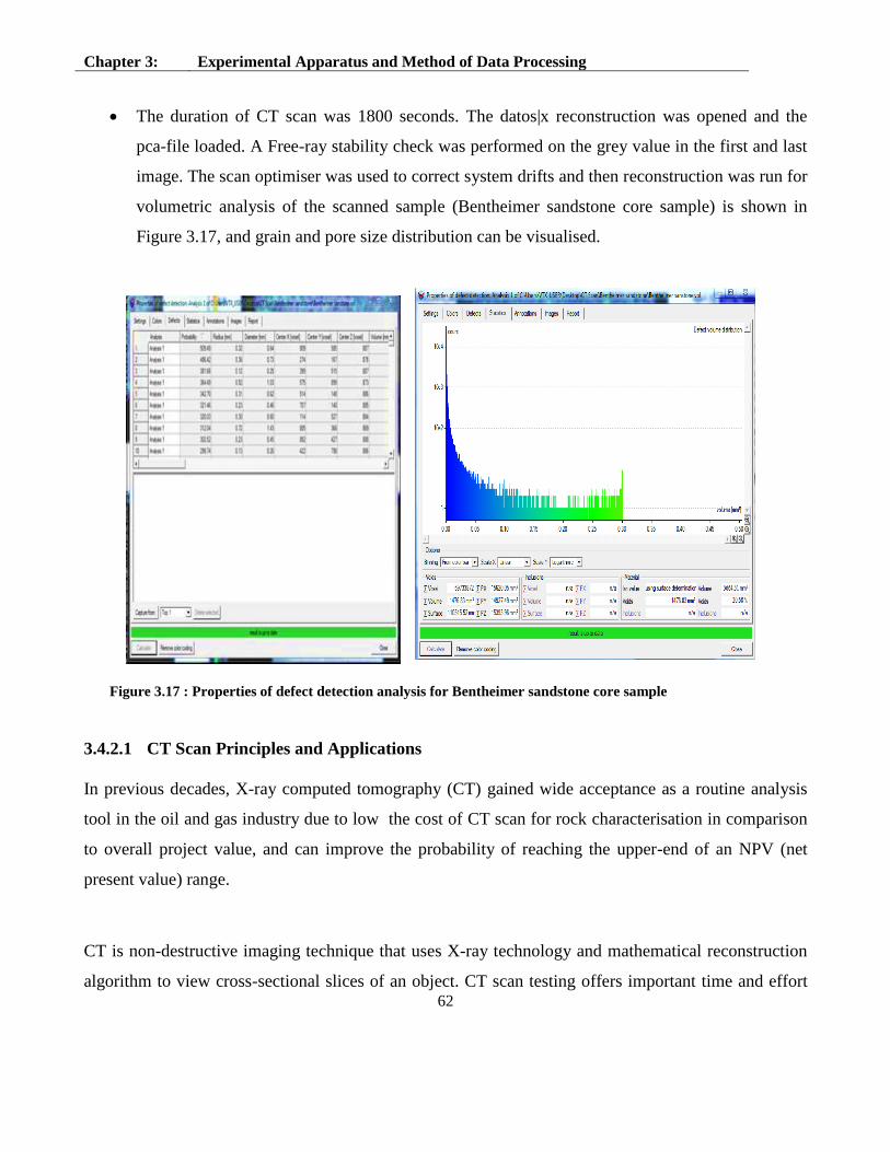
Figure 3.17 : Properties of defect detection analysis for Bentheimer sandstone core sample .............. 62

Figure 3.18 : Flow chart of sectioning to obtain 3D images of porous media [54] .............................. 65

Figure 4.1: Brine density and brine viscosity ....................................................................................... 71

xiv

Figure 4.2: Brine salinity and brine density .......................................................................................... 71

Figure 4.3 :Brine salinity and brine density .......................................................................................... 72

Figure 4.4: Core flow test results for Bentheimer sandstone (10 % NaCl + saturated with 3.5 %) ...... 74


Figure 4.6 : Core flow test results for Bentheimer sandstone (20 % NaCl + saturated with 3.5 %) ..... 76


Figure 4.8 : Core flow test results for Castlegate sandstone (10 % NaCl + saturated with 3.5 %) ....... 79

Figure 4.9 : Core flow test results for Castlegate sandstone (15 % NaCl + saturated with 3.5 %) ....... 81

Figure 4.10 : Core flow test results for Castlegate sandstone (20 % NaCl + saturated with 3.5 %) ..... 82

Figure 4.11 : Core flow test results for Castlegate sandstone (26 % NaCl + saturated with 3.5 %) ..... 83

Figure 4.12 : Core flow test results for Idaho gray sandstone (10 % NaCl + saturated with 3.5 %) .... 85

Figure 4.13: Core flow test results for Idaho gray sandstone (15 % NaCl + saturated with 3.5 % ...... 86



Figure 4.16: Porosity Measurement using PORG- 200 ........................................................................ 90

Figure 4.17 : Porosity Measurement using Liquid Saturating Method ................................................. 93

Figure 4.18: NaCl concentration % & permeability Damage % (Bentheimer sandstone) .................... 95

Figure 4.19: NaCl concentration % & permeability Damage % (Castlegate sandstone) ...................... 96

Figure 4.20: NaCl concentration % & permeability Damage % (Idaho gray sandstone) ..................... 97

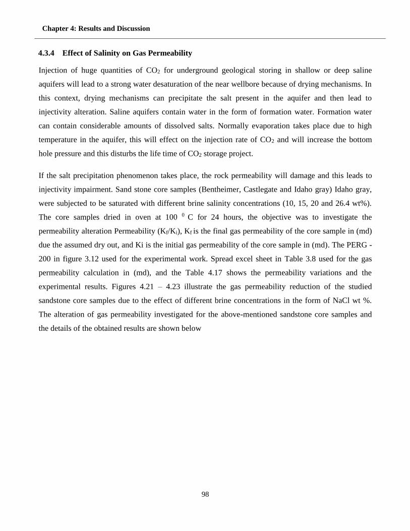
Figure 4.21: the permeability alteration and NaCl % for Bentheimer sandstone ............................... 100

Figure 4.22: the permeability alteration and NaCl % for Castlegate sandstone ................................. 101

Figure 4.23 : the permeability alteration and NaCl % for Idaho gray sandstone ................................ 102

Figure 4.24: the relationship between the porosity and brine permeability ........................................ 104

Figure 4.25: the relationship between the porosity and gas permeability of the studied rocks........... 105

Figure 4.26: Histogram and scan optimiser for Castlegate sandstone. .............................................. 107

Figure 4.27: Properties of defect detection analysis for Castlegate sandstone core sample. .............. 107

Figure 4.28: Histogram and scan optimiser for Idaho gray sandstone. ............................................... 108

Figure 4.29: Properties of defect detection analysis for Idaho gray sandstone core sample. ............. 109

Figure 4.30: Visualisation of the pore spaces for porosity calculation (Bentheimer sandstone),

Porosity = 20.7 % ................................................................................................................................ 110

Figure 4.31: Visualisation of the pore spaces for porosity calculation (Castlegate sandstone), Porosity

= 24.3 % .............................................................................................................................................. 110

xv

Figure 4.32: Visualisation of the pore spaces for porosity calculation (Idaho gray) sandstone),

Porosity = 24.6 % ................................................................................................................................ 111

Figure 4.33: Wall thickness and 3D image of the saturated brine Idaho gray core sample ................ 112

xvi

List of Tables

Table 2.1 : Main criteria for site selection[16] ...................................................................................... 11

Table 2.2 : the worldwide storing capacities evaluations[17] ............................................................... 12

Table 2.3 : Storage rates of three industrial-scale CO2 sequestration projects[20] ............................... 13

Table 2.4 : Classification of reservoir permeability .............................................................................. 21

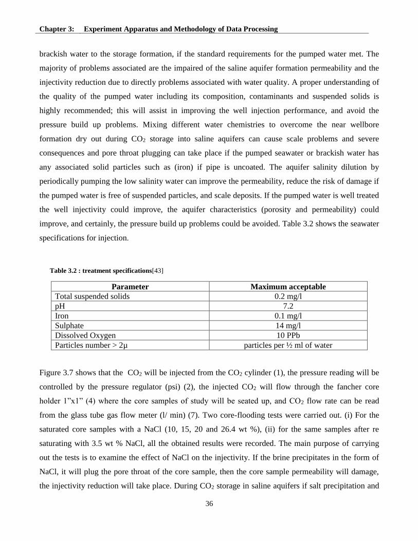
Table 3.1 : Water salinity based on dissolved salts ............................................................................... 33

Table 3.2 : treatment specifications[37] ................................................................................................ 36

Table 3.3: Sample data of core flooding tests ....................................................................................... 40

Table 3.4 : Errors and accuracy of the rig components ....................................................................... 41

Table 3.5 : Spread sheet for grain volume calculation ......................................................................... 47

Table 3.6 : porosity determination by liquid saturating method (Bentheimer sandstone ..................... 48

Table 3.7: Liquid permeability spread sheet for Idaho gray sandstone sample .................................... 53

Table 3.8: Gas permeability spreadsheet for Idaho gray sandstone sample.......................................... 54

Table 3.9: Porosity and permeability sample results ............................................................................ 55

Table 3.10 : initial Brine Permeability and Initial Gas permeability .................................................... 55

Table 4.1: Dimensions of the core samples used in the study .............................................................. 68

Table 4.2 : Brine Salinity (wt %) .......................................................................................................... 69

Table 4.3: Brine viscosity ..................................................................................................................... 69

Table 4.4 : Brine density and specific gravity ...................................................................................... 70

Table 4.5: Brine viscosity and density .................................................................................................. 71

Table 4.6: Brine salinity and density .................................................................................................... 71

Table 4.7: Brine viscosity and salinity .................................................................................................. 72

Table 4.8 : Core flooding test results for Bentheimer sandstone (10 % NaCl + saturated with 3.5 %) 73

Table 4.9: Core flow test results for Bentheimer sandstone (15 % NaCl + saturated with 3.5 %) ....... 74

Table 4.10 : Core flow test results for Bentheimer sandstone (20 % NaCl + saturated with 3.5 %) .... 75

Table 4.11: Core flow test results for Bentheimer sandstone (26 % NaCl + saturated with 3.5 %) ..... 77

Table 4.12: Core flow test results for Castlegate sandstone (10 % NaCl + saturated with 3.5 %) ....... 79



Table 4.15 : Core flow test results for Castlegate sandstone (26 % NaCl + saturated with 3.5 %) ...... 82

Table 4.16: Core flow test results Idaho gray sandstone (10 % NaCl + saturated with 3.5 %) ............ 84

Table 4.17: Core flow test results Idaho gray sandstone (15 % NaCl + saturated with 3.5 %) ............ 85

xvii

Table 4.18 : Core flow test results Idaho gray sandstone (20 % NaCl + saturated with 3.5 %) ........... 86

Table 4.19 : Core flow test results Idaho gray sandstone (26 % NaCl + saturated with 3.5 %) ........... 87

Table 4.20 : core samples porosities by Helium gas porosimeter ......................................................... 90

Table 4.21 : porosity determination spread sheet by liquid saturating method..................................... 92

Table 4.22 :Bentheimer sandstone core samples bine permeability ..................................................... 95

Table 4.23 : Castlegate sandstone core samples brine permeability ..................................................... 96

Table 4.24 : Idaho gray core samples brine permeability ..................................................................... 97

Table 4.25 : effect of NaCl concentrations on gas permeability ........................................................... 99

Table 4.26: Gas permeability alteration of Bentheimer sandstone ....................................................... 99

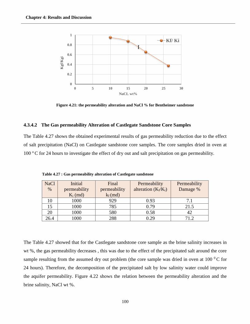
Table 4.27 : Gas permeability alteration of Castlegate sandstone ...................................................... 100

Table 4.28 : Gas permeability alteration of Idaho gray sandstone ...................................................... 101

Table 4.29 : Liquid and gas permeability damage due to halite precipitation. ................................... 103

Table 4.30 : Porosity and brine permeability of the core samples ...................................................... 104

Table 4.31 : Porosity and gas permeability of the core samples ......................................................... 105

Table 4.32 : Shows comparison between porosity computed by helium gas method (A), liquid

saturating method (B) and CT scan method (C) ................................................................................. 112

CHAPTER 1; Introduction

1

1 Chapter 1: Introduction

Currently the energy that uses in daily life comes from four major sources:

i. Fossil fuels (i.e. oil, coal and gas)

ii. Nuclear power

iii. Hydropower

iv. New Regenerative Power (i.e. wind, solar and waste).

Regenerative power sources are probably the cleanest sources of energy but, currently, they cannot

support major industries due to the problem of energy storage. Hydropower is also very clean and

favourable source of energy, however its availability is quite limited and the major barriers have

already been built where possible. Furthermore, the storage of nuclear powers’ waste for a couple of

thousand years is the main problem of using this type of energy source. Mainly CO2 is one of the

greenhouse gases that are responsible for climate change. The consequences and gravity of a changing

climate are currently not well understood, however the price of the worst scenarios to come true is

seem to be so high that politicians have agreed on a system of trading CO2 emission certificates, which

will make the emission of CO2 expensive and hopefully will help to avoid major environmental

changes. Figure 1.1 shows CO2 emissions of industry and power. Saline formations are very deep,

porous and permeable rocks holding water that is useless because of its high salt or mineral content.

Saline aquifers represent promising way for CO2 sequestration. Saline aquifers can be sandstones or

lime stones, but to be a potential reservoir for CO2 storage they must have large enough size,

sufficiently high porosity and permeability, adequate depth: Usually only aquifers below 800 m below

sea level are considered for CO2 storage. In addition to a reservoir rock, an overlying “cap rock “that is

impermeable to the passage of CO2 is required

.


2

Figure 1.1: CO2 Emissions of Industry and Power[1]

Most researches have focused on carbon dioxide due to the large quantity; it represents the highest

percentage of the total greenhouse gas emissions. A promising method to reduce GHG emissions is

geologically store CO2 in the subsurface. Geological storage is the process where CO2 is captured and

subsequently injected into a geological formation in a supercritical state where it is trapped by one or

more trapping mechanisms. This prevents CO2 from leaking through geological seals. Project

monitoring and simulation studies are conducted before, during and after injection to prove that the

carbon dioxide can be trapped within a geological time scale (thousands to millions of years) without

leaking into overlying groundwater reserves, oceans or into the atmosphere. During this period, a

fraction of the CO2 will ultimately dissolve in the formation water and promote geochemical reactions

with the surrounding minerals. These geochemical reactions may alter the cap rock properties and may

thus affect the cap rock integrity. Figure 1.2 shows the contribution of different greenhouses gases to

global warming

54%

5%

3%

15%

2%

1%

12%

2%

6%

Power

Refineries

Ammonia

Cement

Ethylene

Ethylene oxide

Gas Processing

Hydrogen

Iron & steel

% of Emissions

So

urc

e o

f E

mis

sio

ns


3

Figure 1.2: The Contribution of Different Greenhouses Gases to Global Warming[2]

1.1. Risks Associated with CO2 Underground Storage

The risks of CO2 storage in a geological reservoir can be divided into five categories [3]:

CO2 leakage: CO2 passage out of the reservoir to other formations.

CH4 leakage: CO2 injection might cause CH4 present in the reservoir to migrate out of the

reservoir to other formations and possibly into the atmosphere.

Ground movement: Subsidence or uplift of the earth surface because of pressure variations

Displacement of brine: Flow of brine to other formations caused by injection of CO2 in open

aquifers. This may promote the salt precipitation and formation dry out in the near wellbore. This

research focusses on the effect of NaCl precipitation on the injectivity.

70

23

7

Carbon Dioxide

Methane

Nitrous Oxide

% of Contribution to Global Warming

Dif

feren

t G

reen

ho

use

Ga

ses


4

1.2. Contribution to Knowledge

The contribution to this research is to examine the consequence of the salt precipitation (NaCl) on the

injectivity during CO2 injection into Saline aquifers, utilising the designated Experimental set up and

suggest solution to avoid the consequences of salt precipitations.

1.3. Overall Aim

The aim of this work is to examine the effect of Sodium Chloride (NaCl) precipitation on the

injectivity and study how the dilution of brine concentrations by low salinity water (i.e. seawater 3.5 wt

%) could assist in improving the injectivity and avoid the pressure build up problems.

1.4. Objectives

To carry out core flooding tests for (Bentheimer, Castlegate and Idaho gray) sandstone core

samples, which were saturated with dissimilar brine solutions, and examine the effect of brine

concentrations (NaCl wt %) on the injectivity.

To utilise the apparatus for estimating the porosity, the liquid and gas permeability of the stated

core samples.

To analyse qualitatively the porosities of the stated core samples using CT scan.

1.5. Thesis Structure

The thesis contains the following FIVE Chapters:

Chapter 1: Introduction

Chapter 2: This Chapter presents a survey of literatures. It also covers the

definitions, brief history and risk associated with the CO2 storage

Chapter 3: This Chapter demonstrates the experimental apparatus, method of data

processing, which were carried out in this investigation.

Chapter 4: This Chapter discusses the results obtained from the experiment


5

Chapter 5: This Chapter summarises the presented work in this study. The main

contribution is also highlighted with recommendations for future work

Chapter 2: Literature Review

6

2 Chapter 2: Literature Review

2.1 Overview

Worldwide heating is observed as one of the maximum persistent ecological topics fronting current

humanity. This increase in the typical external temperature has been accredited to the greenhouse

result, which has been impaired by the overall rise in atmospheric CO2 is the main greenhouse gas[4].

To struggle these worries, the decrease of carbon dioxide releases with new technologies is needed.

One such method comprises the injection of CO2 into geological formations through a method known

as carbon capture and storage (CCS)[5]. This chapter reviews the physical and chemical mechanisms

leading the injection of CO2 into underground systems. Greenhouse gas releases have become a hazard

for the earth and current culture by means of universal warming. Among others, a major greenhouse

gas, CO2, has been identified as the major provider in terms of increasing usual surface temperature of

the world.

The options to cut CO2 emissions that can be implemented at the necessary scale using current

technology include:

1. Increasing energy efficiency or reducing consumptions.

2. Use of less carbon intensive fuels.

3. Practise of renewable energy bases and / or nuclear energy.

4. Enhancement of natural sinks.

5. Capture the carbon and dispose in engineered sinks.

Geological storage is defined as the procedure of injecting CO2 into geologic formations for obvious

resolution of dodging atmospheric release of CO2, this possibly the most important near period choice.

The charge of attaining bottomless drops in CO2 emissions over the subsequent few periods is

promised to be reduced by geological storage. Figure 2.1 shows the CCS process[6] .


7

Figure 2.1 : The CCS process

2.2 Sources of CO2

The chief cause of anthropogenic carbon dioxide (CO2) release is the burning of fossil fuels. Other

causes are burning of biomass-based fuels in certain industrial procedures, such as the manufacture of

hydrogen, ammonia, iron and steel, or cement. Studies demonstrate that the power and industry areas

joint control present worldwide CO2 releases, accounting for about 60% of entire CO2 releases [7].

2.3 Global Warming and CO2 Emissions

Universal warming is produced by the release of greenhouse gases 72 % of the entirely produced gases

are CO2, 18% Methane, 9 % Nitrous oxide (NOX) [8]. CO2 releases are the greatest significant reasons

of worldwide warming. CO2 is certainly shaped by boiling oil, natural gas, organic – diesel, petrol,

and ethanol. The releases of CO2 have been dramatically enlarged in the last 50 years and are still

rising by almost 0.3% each year. Growing worldwide temperatures are causing a wide choice of

variations. Sea levels are increasing due to warm air development of the ocean, in addition to melting

of land ice. There are two main effects of worldwide heating :(1) Rise of temperature on the

temperature by about (3 – 5 0 C) by the year 2100 (2) Rise of sea level by at least 25 meters (82 ft) by

year 2100. It is well known that a rise in atmospheric concentration of CO2 leads to a rise in the mean


8

atmospheric temperature, that phenomenon is called global warming. If nothing is done to stabilise

CO2, the concentration will reach about 500 ppm within the next 50 years.

Carbon dioxide (CO2) is a greenhouse gas, and thus a rise in atmospheric concentration of CO2 leads to

a rise in the mean atmospheric temperature, a phenomenon that is known as global warming.

Increasing temperatures have been documented around the world, with the largest anomalies being

recorded in the Arctic and Antarctic regions [9] . If nothing is done to stabilise CO2 levels, the

concentration will reach about 500 ppm within the next 50 years. This will lead to an increase in the

mean global temperature by 4 to 6 o C within that same period [9] It is believed that global warming

will have dramatic environmental consequences, such as rising sea levels, loss of fragile ecosystems,

increased intensity of meteorological phenomena, and increased frequency of extreme droughts and

floods [10] . In order to mitigate the effects of global warming, a massive effort must be undertaken to

manage carbon emissions and significantly reduce the amount of CO2 that enters the atmosphere.

Figure 2.2 shows the Origin of anthropogenic CO2 emissions[11] .

Figure 2.2 : Origin of anthropogenic CO2 emissions


9

2.4 CO2 Storage Options

As a technique of CO2 justifying and decreasing greenhouse gas emission from the energy area [1], the

underground storing or geological sequestration (geo sequestration) of CO2 is gradually purchase

respect throughout the world. The storage of CO2 in underground formations is an attractive

greenhouse mitigation choice for large reduction in atmospheric releases[12].

Figure 2.3 : Options for CO2 storage in deep geological underground formations [1]

2.5 CO2 Storage into Saline Aquifer

Deep saline formations are defined as those formations holding water with significant salts or other

compounds to be measured not drinkable or safe to drink. The deposited rock formations soaked with

saline formation waters that are unfitting for social intake or farming use is common. Deep saline

formations have been recommended as promising storing places as of their great quantity and

theoretically large volume[13] [14]. The IEA – GHG guess potential storage volume in deep

formations of 8 x 1011 tonnes CO2 in northwest Europe. In Europe and North America, deep saline


10

formations have been used for injection of risky and safe waste and should be measured as providing

useful information on sequestration[15] . For deep saline formations, one problem is that the potential

efficiency of seals in avoiding pollution of shallower groundwater resources by CO2 is regularly

untested past to CO2 injection. Additional problem is that there are often partial quantities of data

obtainable for site description, needing important calculation charges. Saline aquifers are permeable,

geological formations that contain very salty water and are considered a viable option for disposing of

CO2 emissions because of their large potential capacity for CO2 storing.

The formation of the pore universe that can be employed by injected CO2 is measured by reservoir

heterogeneity, gravity separation and movement and the effectiveness of the injected CO2 [11]. From

industrial opinion, the main concerns of CO2 disposal in aquifers are connected by:

1. The characterisation of suitable aquifer.

2. The accessible storage volume.

3. The attendance of cap rock of low permeability.

4. The injection flow rate of CO2 during the injection [11].

2.5.1 Why Saline Aquifers

Deep saline aquifers offer no economic profit for CO2 injection, but they are common, geographically

connected with fossil fuel sources, and, since it is not necessary to identify and inject directly into

closed structural traps, are likely to have huge storing volumes and appropriate injection sites in close

proximity to power-plant sources of CO2 [16].

In the United States deep saline aquifers have a greater possible storing volume than any other type of

grainy formation, with approximations as high as 500 Gt of CO2 storage [17]. A drawback with deep

saline aquifers is that they are less characterised than petroleum lakes, and a complete characterisation

is desired to confirm the fittingness of the aquifer planned as a storing place[18] .

Saline aquifers as storing locations for CO2 discarding is developing technology, with an increasing

figure of field trials for storing. A public problem for CO2 discarding in aquifers is pressure

preservation. taken care of before reservoir pressure reaches critical limits [19]. Deep aquifers


11

theoretically have CO2-storage capacities adequate to hold many decades’ worth of CO2 emissions, but

estimates of global capacity are poorly controlled, varying from 300 to 10,000 Gigatons CO2 [20].

2.5.2 Reservoir Properties of Saline Aquifers

Saline aquifers are permeable, geological formations that contain very salty water and are considered a

viable option for disposing of CO2 emissions because of their large potential capacity for CO2 storage.

About the ability of saline aquifers to contain CO2 for hundreds of years, they are different from oil

and gas reservoirs in that there is often not a well-defined structural trap. Instead, containment of CO2

will depend on the existence of a confining layer, or cap rock, that extends laterally along the top of the

formation. The analysis of the literature makes it clear that CO2 storage into aquifers is feasible. The

main issue with this technique is the characterisation of the aquifer, which is significant part of the

entire assessment of the aquifer as a dependable long-term CO2 storing site. Hence, the current need is

to improve technologies and strategies to gather adequate information for aquifer characterisation, as

well as to recognize the issues that disturb the volume of aquifers to store CO2. Numerical simulations

can help gain further insight into the CO2 storage process and thus, the factors, which make the process

successful[18]. The Suitable Aquifers should have the following characteristics:

1. Contain saline water (Salinity > 100 g/l) to dodge pampering drinkable water resources.

2. Exceed lowest permeability >500 md, porosity >20%

3. Afford storage depths of 800 m or more (where CO2 will be in a compressed fluid phase and

long way from the ground surface or seabed).

4. Require a least thickness to limit the possible storing areal foot pattern.

Table 2.1 : Main criteria for site selection[21]

High storing volume Good porosity

High storage volume Large reservoir

Effective injectivity High permeability

Safe and secure storage Low geothermal gradient & high pressure

Safe and secure storage Adequate sealing

Safe and secure storage Geological & hydrodynamic stability

Low costs Good accessibility, infrastructure

Low costs Source close to storage reservoir


12

Table 2.2 shows the summary of global storing volume evaluations.

Table 2.2 : the worldwide storing capacities evaluations[22]

Type of formation Volume Estimate Source

Depleted oil and gas

reservoirs ~ 45 Gt

Stevens et al. 2001 : GHGT 6

pp. 278 - 283

Coal-bed methane reservoirs 60 – 150 Gt Stevens et al. 1999 : GHGT 6

pp. 175 - 180

Saline aquifers 300 – 10,000 Gt IEA Greenhouse Gas R&D

programme, 1994

2.6 Trapping Mechanism

Depending on the rock formation and reservoir category, CO2 can be surrounded in the subsurface by a

number of dissimilar mechanisms [5], as discussed further in the following sections. Figure 2.4 shows

different phases of CO2 trapping mechanisms[23].

Figure 2.4 : Trapping mechanisms for CO2 storing in deep saline aquifers A) structural trapping, B) capillary

trapping, C) dissolution and D) mineral trapping


13

2.7 CO2 Injection Approaches

Studies were carried out on CO2 stream performance on the process facilities within relevant

thermodynamic conditions. Main constituents and environments leading whether large volumes of

supercritical CO2 can be securely, dependably and strongly injected into and stored within a saline

aquifer, were examined by modelling many injection methods. The strategies are:

1. Typical CO2 injection

2. CO2 – brine surface mixing

3. CO2 – water surface mixing

4. CO2 – alternating brine (CAB)

2.8 Present and Scheduled CO2 Projects

There are four large-scale developments on the planet, which restore anthropogenic CO2 [24]:

Sleipner (Norway)

In Salah (Algeria)

Weybum- Midal (Canada)

Snohvit (Norway)

In terms of cumulative volume injected and knowledge of CO2 storing, the most important are Sleipner

and In Salah. Table 2.3 shows the largest CO2 storage projects in the world.

Table 2.3 : Storage rates of three industrial-scale CO2 sequestration projects[2]

Name of the project Project starting date Storing rate

Sleipner Since 1996 1 million tonne CO2/year

Weyburn Since 2000 500,000 + tonne CO2/year

In Salah Since 2004 1.2 million tonne CO2/year

2.9 Risks Posed by CO2 Geological Storage

Similar with any human activity, there are definite hazards related with CO2 geological storing. Hazard

in its engineering explanation is the creation of an event to happen and the consequences of the event-

taking place. Henceforward, since consequences are extremely dependent on site and time, the

following discussion will address only the various events that may take place and their potential

consequences; furthermore, only the risks associated with CO2 storage will be discussed as the risks


14

connected with surface and injection/production facilities are well understood[25]. Risks associated

with CO2 geological storing may happen during the injection phase and/or afterwards.

CO2 escape (leakage) poses different risks because of its possible consequences. Leakage is possible

because, besides the pressure force that acts on CO2 during injection, buoyancy acts on CO2 at all

times, pushing it upwards, and, if a pathway is available, CO2 will flow along this pathway. Thus,

leakage is possible during both injection and afterwards. From the point of view of retention efficacy

and safety, CO2 storage through static and hydrodynamic mechanisms is of most fear because CO2 is

mobile and may escape into overlying formations and perhaps to shallow groundwater. Storage

through residual-gas and mineral trapping is of no worry because the CO2 is immobilised, either in its

own chemical form or in a different one. Water saturated with CO2 is somewhat heavier (by 1-2%)

than unsaturated water and its undesirable buoyancy will tend to drive it towards the bottom of the

storing aquifer if definite circumstances for the onset of free convection are being met[26] and finally

down dip in the aquifer. Carbon dioxide adsorbed onto the coal surface will be immobile as long as the

pressure does not drop, which would be the case if the coals were subsequently mined. Only mobile

free-phase CO2 may pose risks due to its buoyancy, which will move it up from its storage unit if a

pathway is found, such as open faults and fractures, and defective wells[15].Local consequences of

CO2 leakage can be short-term or long term, and fall into three categories: health, safety and

environmental issues.

2.9.1 Salt Precipitation and Dry out in the near- Wellbore

The most significant physical mechanism of CO2 injection into deep saline aquifers is the combined

dissolution of CO2 and water, which means that CO2 can dissolve in formation brine and at the same

time, formation brine can evaporate into CO2. During the injection of dry CO2, the salt will finally

fully saturate the brine producing the salt to start precipitating as a solid phase figure 2.5. This dense

precipitation might expressively decrease the porosity and permeability of the porous medium. This

problem was first discovered around producing wells in gas reservoirs where high salinity brine is

present [27]. This research focuses on the salt precipitation phenomenon in the near wellbore, if salt

precipitation takes place, it will effect on the aquifer properties (porosity and permeability) and the

well injectivity of the CO2 injectors will be reduced.


15

Figure 2.5 : Schematic of CO2/water mutual dissolution in porous media [39]

The key physical devices touching the dry-out and salt precipitation procedure comprise: (1) the

injection of CO2 will move the brine away from the injection well. (2) The brine will evaporate (3) the

Up flow of CO2 will take place due to the effect of buoyancy. (4) Due to the capillary pressure

gradients the Backflow of brine toward the injection well will occur, and (5) Molecular diffusion of

dissolved salt.

The impairment of the injectivity has been found to depend on the mobility of the brine phase, with a

potentially high impairment at high water saturations. Salt precipitation in the investigated field

samples led to a strong decrease of permeability in cases where the brine phase was above residual

saturation, i.e. with a mobile brine phase, which means that above residual water saturation there is a

potential risk of injectivity loss[23] .

From capacity, point of view deep saline aquifers offer the highest potential for CO2 storing.

Vaporisation of water needs specific consideration, as it is the main source of salt precipitation

problems. Research described by Bacci et al aimed to provide variations in porosity and permeability

due to salt precipitation (water vaporisation). CO2 core flooding experiments were conducted on a St.


16

Bees sandstone core with completely saturated saline water gaining numerous levels of alteration due

to halite scaling. Porosity decrease ranged from around 4 to 29 % of the initial value and the

permeability damages were from 30 to 86 % [28].The objective of this work is to examine the effect of

bine concentrations on the injectivity and how the dilution by seawater can assist in improving the

liquid and gas permeability the injectivity as well.

Permeability change has been measured scientifically for four type of rocks typical of aquifer storing

rocks (Vosges Sandstone 1, Vosges Sandstone 2, Lavoux limestone 1 and Lavoux limestone 2). Each

sample was completely saturated with a brine of dissimilar salt composition (KCl, NaCl and Keuper

brine, a mixture of salt representative of the Paris Basin brine aquifer) and different salinity up to 250

g/l by Peysson et al [29].The samples were then totally dried in an oven at measured temperature and

with vapour removal. A clear linear reduction in permeability was observed. Local study showed that

the salt precipitation is localised near the surface of the sample and pores are plugged by solid

precipitations, the change of permeability made by drying of brine in porous media.

The investigational work by Müller et al[30] displayed a 60% permeability decrease due to halite

precipitation over the whole pore system of the Berea sandstone core after 32 hours of flooding. Non-

stop injection of dry supercritical CO2 into saline aquifers could lead to the development of a dry-out

zone in the area of the injection well within which hard salt is precipitated André et al[31]. This salt

precipitation results in reduced porosity and permeability, and accordingly, the well injectivity is

severely decreased.

2.10 Approaches to Restore the Well Injectivity

While scheduling a CO2 injection structure the greatest critical factors, apart from containment security

and satisfactory storing volume are the injectivity of the potential reservoir unit and storage efficiency.

Optimisation of these factors is essential to maximise storage capacity and improve the economics of

an injection operation. The injectivity is defined as the ability of a geological formation to accept fluids

by injection through a well. The main limiting factor for injectivity is the bottom-hole injection

pressure, which should not exceed the formation fracture pressure. It is common for regulators to set a

criterion for the maximum injection pressure that is somewhat less than this e.g. 90% of the fracture


17

pressure. According to the well testing equations, critical restrictions controlling the bottom hole

pressures around an injection well are:

The injection rate of CO2

The aquifer permeability

The relative permeability to CO2

The net pay of the completed interval

Viscosity contrast between brine and CO2 (mobility) and compressibility.

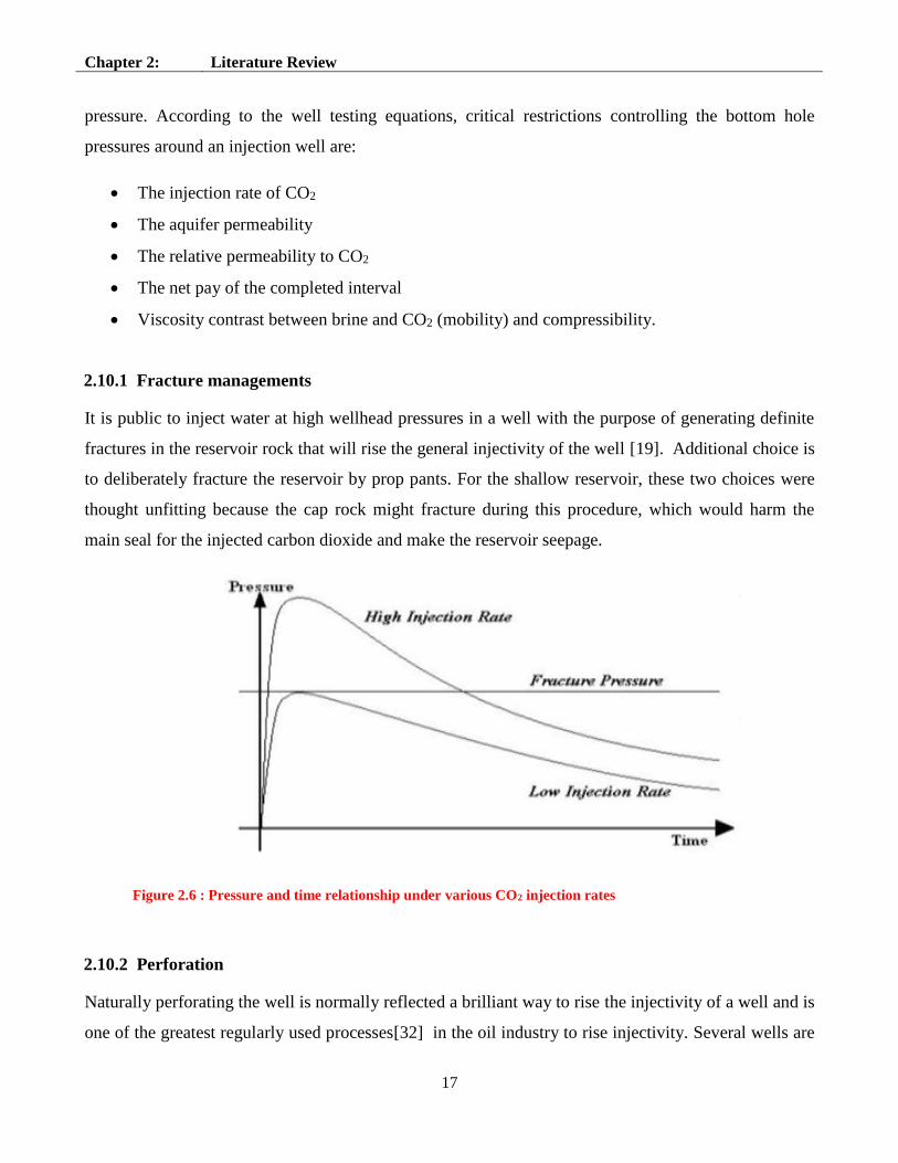
2.10.1 Fracture managements

It is public to inject water at high wellhead pressures in a well with the purpose of generating definite

fractures in the reservoir rock that will rise the general injectivity of the well [19]. Additional choice is

to deliberately fracture the reservoir by prop pants. For the shallow reservoir, these two choices were

thought unfitting because the cap rock might fracture during this procedure, which would harm the

main seal for the injected carbon dioxide and make the reservoir seepage.

Figure 2.6 : Pressure and time relationship under various CO2 injection rates

2.10.2 Perforation

Naturally perforating the well is normally reflected a brilliant way to rise the injectivity of a well and is

one of the greatest regularly used processes[32] in the oil industry to rise injectivity. Several wells are


18

even re - perforated to raise injectivity or throughput. However, the high danger of probably harmful

watching equipment in the well hindered the application of this choice.

2.10.3 Acid Management

Acid managements are frequently useful to inspire wells. The possible achievement of such

managements is normally difficult in the petroleum reservoirs. Additionally, for an ideal treatment,

data concerning the environment of the hindering solid would be essential to choose the type,

concentration, and shot size of the acid plus the additional chemicals required for the programme.

Besides, the intensive care equipment in the well is superficial to definite acids, particularly organic

acids. Organic acids are characteristically the preferred acid type for acid treatments for the reason that

they are slight, less corrosive to iron and have the possibility to keep iron that was mobilised by the

decomposition developments in resolution [33].

2.11 Optimisation of CCS Costs

Figure 2.7 the optimisation of CCS costs.

Figure 2.7 : The scheme of cost optimisation of CCS[34]

Optimisation CCS Costs

Capture

Costs

Transport

Costs

Storage

Costs

Reservoir

Parameters Well

Parameters

Numerical

Parameters


19

2.12 Rock Properties

For flow simulation in oil and gas reservoirs, the porosity and permeability are considered the key

properties. Porosity is defined as the ratio of the pore volume to the bulk volume. In the oil and gas

industry the porosity is classified as absolute and effective porosity, the petroleum engineers are

interested in the effective porosity as it represents the interconnected void space. More details about

porosity and its measurements are covered in Chapter 3.

Figure 2.8 : (a) Cubical packing, (b) rhombohedra, (c) cubical packing with two grain sizes, and (d) typical sand

with irregular grain shape

2.13 Classification of Porosity

Throughout sedimentation, some of the pore spaces originally developed and became isolated from the

other pore spaces by many digenetic processes such as cementation and the compaction. Therefore,

several of the pores will be interconnected, while other will be very isolated. This lead to two

dissimilar classes of porosity, namely, total (absolute) and effective, depending upon which pore

spaces are measured in defining the volume of that sample; irrespective of whether those void spaces

are interconnected or not.


20

2.13.1 Effective Porosity

The effective porosity (Φe), also called the kinematic porosity, of a porous medium is defined as the

ratio of the pore volume to the bulk volume. The definition of effective (kinematic) porosity is linked

to the concept of pore fluid displacement rather than to the percentage of the volume occupied by the

pore spaces. The pore volume employed by the pore fluid that can circulate through the porous

medium is less than the total pore space, and, therefore, the effective porosity is always lesser than the

total porosity.

2.13.2 Absolute Porosity

It represents the total void space (connected and interconnected pores) to the bulk volume of the core

sample and it dimensionless quantity could be reported as fraction or percentage. For the absolute

porosity measurement, assuming that the soil system is composed of three phases:

Solid phase, has volume Vs

Liquid phase (water) has volume Vl

Gas phase (air) has volume Vg

Then the pore volume of the sample (Vp) = Vl + Vg

The total volume of the sample (Vt) = Vs + Vl +Vg, and the sample porosity is determined by:

Φt =VP

Vt=

Vl + Vg

Vs + Vl + Vg

(2.1)


21

2.14 Permeability

In oil and gas industry, the permeability is defined as ability of the fluid to flow through porous

medium, and according to Darcy’s law, the permeability is measured in Darcy. The permeability is

classified to absolute, effective and relative permeability. The absolute permeability is the

measurement of the core sample permeability in the presence of one phase fluid while the effective

permeability is the measurement of the permeability in the presence of more than one phase fluid. The

relative permeability is the ratio of the effective permeability to the absolute permeability. Normally

the permeability depends on the porosity, the higher the porosity the higher the permeability. The

connectivity of the pores depends on the size of the grains, the shape of the grains and the grain size

distribution. For the permeability of the reservoir rocks, the following points are noticeable:-

Higher porosity means high permeability

Small grains, small pores and small pore throats give low permeability

High rock compaction gives low porosity and low permeability

Table 2.4 : Classification of reservoir permeability

Permeability in (mD) Permeability Classification

Less than 10 Fair

10 - 100 High

100 - 1000 Very High

Higher than 1000 Exceptional

In general, the permeability depends on

The rock porosity

The flow paths connectivity of the rock

The pore geometry of the rock

The reservoir heterogeneity. The permeability is calculated by Darcy’s equation (3.4)


22

(a) Pore Space of Rock Grains

(b) Permeability is an indication of how easy is

for the fluids to flow through the medium

Figure 2.9 : Permeability is an indication of how easy it is for the fluids to flow through the medium [47]

2.15 Saturation

Saturation is another essential rock property. Saturation is defined as that fraction, or percent of the

pore volume occupied by a particular fluid (oil, gas or water). This property is expressed

mathematically by the following relationship. Fluid saturation total = (volume of the fluid) / (pore

volume). Applying the above mathematical model of saturation to each reservoir liquid provides:

So (oil saturation) = (oil volume)/ (pore volume)

Sg (gas saturation) = (gas volume)/ (pore volume)

Sw (water saturation) = (water volume)/ (pore volume)

Where: So + Sg +Sw = 1.0

2.16 Well Injectivity

The well Injectivity is an essential technical and economic concern for CO2 geological storing

projects, meanwhile very huge volumes of CO2 must be stored. For long period of storing, water

vaporisation has been reported as the chief reason of permeability damages around several gas


23

producing wells; particularly in high pressure, high temperature reservoirs which are categorised by

very high salinity brines[21][35].

The high storing capacity alone is not sufficient for a reservoir to be considered as a suitable storage

site. There are two other requirements; high, injectivity and safe containment. The reservoir injectivity

measures the ability of a reservoir to accept CO2 at maximum possible flow rate before losing its

mechanical integrity (keep average reservoir pressure less than critical pressure). The well injectivity

(or well capacity), on the other hand, measures the ability of a single injection well to accept CO2 into

a formation without reactivating existing faults or creating new fractures[36]. To ensure this, the

injection pressure (the well flowing pressure) must not exceed 90% of fracturing pressure considering

all others regulatory factors with regard to the injection such as maximum pump pressure [37]. A basin

pilot injectivity test is normally required to offer a straight amount of the reservoir injectivity. The

following equation can be used for injectivity determination:-

Injectivity =QCO2

PInjection − PReservoir

(2.2)

Where:

Q CO2 = the volumetric flow rate of CO2

P Injection = the injection pressure of CO2

P reservoir = the reservoir pressure.


24

2.17 CT Scan

CT scans “Computed tomography” are commonly used for measuring three-dimensional features, but

old-style CT scans produce two-dimensional cross-section views of substances. CT scanning offers

chance to examine particle and pore connections at any time and location within the sample. A CT

scan comprises of two key processes: data collection and image reconstruction. The data collection

phase of a CT scan happens after the object is viewed with x-rays from many different directions.

Reconstructing a CT scan gives a picture of the internal structures of an object. In this research the CT

scanning was used to determine the porosity of (Bentheimer, castlegate and Idaho gray) sandstone core

samples using Volume Graphic Software. The pore and grain size distribution of the stated core

samples were Visualised. Petroleum engineers utilized CT for fluid-flow experiments and

sedimentologists for the analysis of sedimentary structures [38]. CT scanners have been used in petroleum

industry as an effective tool for analysing the reservoir rocks for more than 30 years[39] .

An x-ray image is a picture of the x-ray linear attenuation coefficient of an object, which is related to

the density of an object [40] .The digital image formed during the x-ray CT process, provides an

internal cross-section, in which different materials can be distinguished. Over the last decade,

researchers have many experiments using of x-ray CT scanning technologies to quantity physical

density, void ratio, and soil collective size distribution [40]. The benefits of x-ray CT scanning

comprise time- savings and negligible sample disruption. Nielsen [41] demonstrated that x-ray CT

scanning can provide collective size data stable with traditional testing approaches but deprived of the

time-consuming sample preparations involved with traditional tests. In specific, CT scan testing offers

important savings in time and energy once likened to sample coupon preparation techniques. The non-

destructive nature of CT scanning permits the same soil sample to be scanned many different times.

Since the sample is not affected by the testing procedure.


25

2.18 Summary

After reviewing the options for the geological storage of CO2 into underground systems and

having an overview of the storage sites worldwide, it is noticeable that depleted oil and gas

reservoirs and deep aquifers are the most attractive storage sites for CO2 sequestration.

CCS is an important process to mitigate emissions of CO2 into the atmosphere. However, lack

of incentives and regulatory regimes are key barriers that need to be overcome.

It is not evident that all cap-rocks will contain CO2 safely, since the interfacial tension may be

lower and the contact angle higher, implying a lower entry pressure. Furthermore, the CO2 in

solution could react with the cap-rock, eroding escape paths[42].

CO2 may also migrate back up through the well after ending the injection process. In case of

sealing failure due to fracture that takes place because of pressure build up problem, the CO2

can escape to the upper formation and might contaminate the water of that formation.

It is proved by CO2 – EOR that the CO2 storage process is feasible and the recent CO2 storage

operations at Sleipner and In Salah are good examples.

Economics will possibly affect applications, as there is no return value of stored CO2.

Confirming adequate injectivity and dodging huge pressure rises at the well and in the

underground formation is essential to allow large-scale storing deprived of fracturing the rock

or producing intrusion into drinking water.

CT scan may offer motivating qualitative interpretations of the internal construction of core

samples, elements and openings. It can be used for porosity determination using (VG) Volume

Graphics Software.

Chapter 3: Experiment Apparatus and Methodology of Data Processing

26

3 Chapter 3: Experiment Apparatus and Methodology of

Data Processing

This Chapter describes the Experimental apparatuses procedures and methodology that carried out

throughout these investigations. The experiment was designed to study the effect of salt precipitations

in terms of sodium chloride (NaCl) on the liquid and gas permeability of sandstone during the storage

of CO2 in saline aquifers and how the permeability impairment will effect on the injectivity. The

relationship between the brine density, viscosity and salinity also considered in this experimental work.

Sea salt was used to dilute different brine salinity concentrations, this demonstrated that the seawater

could be utilised and pumped to the CO2 injectors to avoid the salt precipitation and near wellbore

formation dry out and overcome the pressure build up problems. The injected water should be treated

properly in order to meet the required technical specifications. All the utilised apparatus are explained

in the next sections.

This work of the Chapter is divided into three sections as follows: Phase-I carrying out simple core

flooding tests for different sandstone core samples which were saturated with different brine

concentrations, the flow tests were carried out to measure the carbon dioxide flow rate in (l/min)

through the studied sandstone core samples at different injection pressures in (psi) . Phase - II Utilising

the laboratory apparatus to calculate the porosity, liquid and gas permeabilities of the sandstone core

samples (Bentheimer, Castlegate and Idaho gray). Phase - III Qualitative analysis of the core samples

porosities using the high class CT scanning. Figure 3.1 illustrates the work plan of the thesis.

The core flooding tests carried out to investigate the effect of brine (NaCl) on the stated sandstone core

samples. The setup in Figure 3.8 was designed to work under pressure (0 – 60 Psig) and temperature of

25 0 C, the setup is simply composed of Fancher core holder for core samples dimension (1”x1”),

compressor system that allows injecting the carbon dioxide gas (CO2) in (l/min).


27

Figure 3.1: Thesis work plan

Sample Preparation

(Sandstones and Brine Concentrations)

(Section 3.1)

Phase – I

Core Flooding Test

(Section 3.2)

Phase – II

Porosity and Permeability

(Section 3.3)

Design of

Experimental Rig

(Section 3.2.1)

Description of

Apparatus

(Section 3.3.1)

Description of

Apparatus

(Section 3.4.1)

Methodology of

Measurements

(Section 3.2.2)

Errors and Accuracy

(Section 3.2.3)

Methodology of

Measurements

(Section 3.3.2)

Errors and Accuracy

(Section 3.3.3)

Methodology of

Measurements

(Section 3.4.2)

Errors and Accuracy

(Section 3.4.3)

Results and Discussions

(Chapter 4)

Salinity

(Section 3.1.1)

1.1) Viscosity

(Section 3.1.2)

Density

(Section 3.1.3)

Errors and Accuracy

(Section 3.1.4)

Phase – III

CT-Scanner

(Section 3.4)


28

3.1. Sample Preparation

Samples used for experiments should be clean and dry. Irregularly shaped samples can be used for

grain volume determination; however, if porosity is required, the samples must conform to the

requirements of the bulk volume apparatus to be used. A serious issue in utilising laboratory

measurements is the representativeness of the sample under investigation, i.e., to what degree the

results of laboratory data can be extended to characterise large underground rock volumes, or to

determine their actual value at a level of certainty needed to make economic decisions leading to

reservoir development and production. In dealing with petro physical properties, it is crucial to define

the investigation scale, which extends from a small scale a single core, a well or a group of wells to a

single reservoir up to a regional geological scale.

Direct core measurements only grant information on a small scale, and can be extended to a larger

scale by the aid of properly integrated and calibrated indirect measurements and taking into account the

possible heterogeneity and discontinuity of the reservoir by means of geo statistical methods. In

general, the most difficult part of any petro physical measurement is to determine the actual values at a

level of certainty needed for making economic decisions regarding the possible development or the

production management of hydrocarbon reservoir. The core samples that are used for laboratory

measurements are usually taken from the subsurface rock using several techniques (i.e. rotary, sidewall

and cable-tool coring).

Different Sandstone Core Samples

Three types of sandstone core samples were selected for this study; the selection was based on good

porosity and good permeability. The selected sandstone types are (Bentheimer, Castlegate and Idaho

gray). These sandstone samples have good porosity and good permeability, and they are very good

candidates for CO2 underground storage. The core samples dimensions (diameter and length) and their

weights are recorded. Figure 3.2 illustrates the core samples of the study.


29

:

Figure 3.2: Different Types of Sandstones (a) Bentheimer, (b) Castlegate and (c) Idaho Gray

Different Brine Concentrations

In Saline aquifers, the high salinity in PPM or in wt% is expected. Therefore in this study different

brine solutions in wt % were prepared (10, 15, 20 and 26.4 wt %), the concentrations were prepared

using Sodium chloride (NaCl). For dilution purpose, sea salt was used to prepare 3.5 wt % brine

solution. Note that 1.0 wt % equals 10,000 PPM. Concentration is very important property of solutions

that must addressed. In this research, sea salt was used to prepare 3.5 wt % brine solutions to dilute the

different brine concentrations. The objective was to investigate the reliability of the dilution in improve

the core samples permeability and injectivity. The refractometer was used to measure the different

brine concentration in wt %.

One of the important physical mechanisms of CO2 injection into deep saline aquifers is the mutual

dissolution of CO2 and water, which means that CO2 can dissolve in formation brine and at the same

time, formation brine can evaporate into CO2. During the injection of dry CO2, the salt that contains

halite mainly will eventually fully saturate the brine causing the salt to start precipitating as a solid

phase. This solid deposition could significantly reduce the porosity and permeability of the porous

medium. Figure 3.3 shows the brine solutions in % for this study.

(a) (b)

(c)


30

Figure 3.3: Brine solutions in (wt %)

3.1.1 Salinity Measurement

The measurement of the total dissolved salts in seawater is called salinity. In this research the

refractometer in Figure 3.4 was used for measuring the brine salinity in wt %. It can exactly measure

the amount of refraction that is caused by the density. The instrument is temperature compensated.

This means that the temperature effects on refraction can be ignored for these measurements, and the

salinity can be read directly from the refractometer. The refractometers are low-cost, simple devices

that are popular in a multitude of applications. They are popular because they are easy and convenient

to use.

Hand-held refractometers work according to the same basic principles and design considerations

outlined above. However. The Refractometers are limited in terms of accuracy and applicability

because:

The Refractometers utilise natural (white) light

There is no way to control temperature

Light must be transmitted by the sample


31

Figure 3.4 : Refractometer gives the salinity in (wt %)

Usually, salinity is expressed in parts per thousand (ppt), regularly written as º/ºº. The salinity is also

expressed percent (%). For example, if 1000 g of seawater contains 35 grams of dissolved salt, the

salt solution will be a 3.5% or a salinity of 35 parts per 1000 (35º/ºº).

3.1.2 Viscosity Measurement

The resistance of fluid to flow is called fluid viscosity. In this study, rotational electrical viscometer

type was used for dynamic viscosity measurement. Different viscometers are used for viscosity

determination

In this, work the viscosities of brine solutions were determined using the OFITE Model 800 8-Speed

Electronic Viscometer illustrated in Figure 3.5. In other to determine the viscosities of different brine

concentrations in PPM, the viscometer was calibrated in order to get accurate measurements.


32

Figure 3.5 : Electronic Rotational Viscometer

Viscosity defines a fluids resistance to flow. Dynamic viscosity (sometimes referred to as Absolute

viscosity) is obtained by dividing the Shear stress by the rate of shear strain. The units of dynamic

viscosity is Force / area x time. The Pascal unit (Pa) is used to describe pressure or stress = force per

Shear stress = Ib/100 ft2

Shear rate y = RPM x 1.703 1/sec

Dynamic viscosity = (Ib/100 ft2) / (1/sec) = Ib .sec/ 100 ft2

µ = lb -sec/100 ft2, 1.0 lb.s/ft2 = 47880.26 Centipoise.

The viscosity can by calculated by:

μ = KFθ

rpm

(3.1)


33

Where

µ is the brine viscosity in cP

K = 300, F is the spring factor equals 1,

θ is the dial reading (shear stress)

The procedure for viscosity determination is as the following:

Mixing the sample on the “STIR” setting for 10 seconds until reaches the target temperature

Rotate the knob at the intended speed setting until stabilisation. When the dial reading

stabilises, record the reading and the temperature. Repeat this step for any other speeds that

your test requires

Repeat the above step for any other speeds and record the obtained data.

3.1.3 Density

The density of certain fluid is defined as the mass of that fluid per unit volume. The unit of density is

expressed as kilogram per cubic meter. For example, water at a temperature of 20 °C has a density of

998 kg/m3 occasionally the term ‘Relative Density’ is used to define the density of a fluid. Relative

density is the fluid density divide by the density of water, which equals 1000 kg/m3. Water at a

temperature of 20 °C has a Relative density of 0.998. Brine is a solution of salt (Halite) NaCl in water.

In different contexts, brine may refer to salt solutions ranging from about 3.5 wt% (a typical

concentration of seawater) up to about 26.4 wt% (a typical saturated solution, depending on

temperature). Table 3.1 shows the salinities of different dissolved salts.

Table 3.1 : Water salinity based on dissolved salts

Fresh water Brackish water Saline water Brine

< 0.05 % 0.05 – 3 % 3 – 5 % >5%

The brine density is measured by mud balance. The mud balance is mud scale device, also known that

is used to measure the density of the drilling in ppg (Ib/gallon) , cement or any type of liquid. Figure

3.6 illustrates the mud balance for measuring the fluid density. It consists of a graduated beam with a


34

bubble level and a weight slider along its length and a cup with a lid on one end. The cup is used to

hold a fixed amount of fluid so it can be weighed. A slider-weight can be moved along the beam, and a

bubble indicates when the beam is level. Density is read at the point where the slider-weight sits on the

beam at level.

Sodium chloride (NaCl) is not strictly a scale. The mixing of incompatible waters forms most oilfield

scales. Salt, however, is a self-scaling phenomenon requiring only changes in physical conditions to

precipitate. It is also, generally, a gas well problem, for reasons that become apparent when looking at

the mechanism of salt deposition. There are two mechanisms working to cause precipitation of salt;

firstly, evaporation of fresh water from formation brine into the producing gas, which increases, brine

salinity, and secondly, changes in pressure and temperature, which can reduce the solubility of the salt

in the brine. Either or both can result in the brine becoming salt saturated so that the salt precipitates

out. Precipitated salt is generally nearly 100 wt % NaCl.

Figure 3.6 : Mud Balance scale device


35

Figure 3.6 shows the mud balance that is used for fluid density measurement. The arm is graduated and

permits accurate measurements to within ±0.1 pounds per gallon. The measurement procedure

summary is as the following:

i. The mud balance needs to be placed on a flat level surface.

ii. The temperature of the fluid needs to be measured and recorded.

iii. The dry and clean cup needs to be filled to the top with the intended mud sample.

iv. The lid needs to be placed on the cup, and set it with a gentle twisting motion.

v. The hole in the lid needs to be covered with a finger and wash all mud from the outside of the

cup arm.

vi. The balance needs to be placed Place on the knife-edge and move the rider along the outside of

the arm until the cup and arm are balanced as indicated by the bubble.

vii. At the edge of the rider toward the mud cup, read the mud weight in ppg.

viii. After each use, the mud balanced needs to be cleaned and dried properly.

3.1.4. Errors and Accuracy

Salinity

o The accuracy and precision is limited by the size and optical arrangement. Sample

temperature range 5-90 °C. Sample volume 0.30 ml and the temperature sensor

accuracy ±1 °C (5 – 40 °C). The error percent of the reading is ±0.2.

Viscosity

o Speed accuracy (RPM) = 0.1, Minimum viscosity @600 RPM = 0.5 cP, Maximum

viscosity @600 RPM = 33, 000 cP.

Density

o The density of the fluid can be measured by mud balance. The arm is graduated and

permits accurate measurements to within ±0.1 pounds per gallon or ±0.01 specific

gravity.

3.2 PHASE-I: Core Flooding Tests

The formation dry-out and precipitation of salt near the injection well is expected to take place during

CO2 in injection in Saline aquifers. The precipitated salts will reduce formation porosity, permeability,

and injectivity. One approach to delay the onset of this phenomenon is periodic flush of seawater or


36

brackish water to the storage formation, if the standard requirements for the pumped water met. The

majority of problems associated are the impaired of the saline aquifer formation permeability and the

injectivity reduction due to directly problems associated with water quality. A proper understanding of

the quality of the pumped water including its composition, contaminants and suspended solids is

highly recommended; this will assist in improving the well injection performance, and avoid the

pressure build up problems. Mixing different water chemistries to overcome the near wellbore

formation dry out during CO2 storage into saline aquifers can cause scale problems and severe

consequences and pore throat plugging can take place if the pumped seawater or brackish water has

any associated solid particles such as (iron) if pipe is uncoated. The aquifer salinity dilution by

periodically pumping the low salinity water can improve the permeability, reduce the risk of damage if

the pumped water is free of suspended particles, and scale deposits. If the pumped water is well treated

the well injectivity could improve, the aquifer characteristics (porosity and permeability) could

improve, and certainly, the pressure build up problems could be avoided. Table 3.2 shows the seawater

specifications for injection.

Table 3.2 : treatment specifications[43]

Parameter Maximum acceptable

Total suspended solids 0.2 mg/l

pH 7.2

Iron 0.1 mg/l

Sulphate 14 mg/l

Dissolved Oxygen 10 PPb

Particles number > 2µ particles per ½ ml of water

Figure 3.7 shows that the CO2 will be injected from the CO2 cylinder (1), the pressure reading will be

controlled by the pressure regulator (psi) (2), the injected CO2 will flow through the fancher core

holder 1”x1” (4) where the core samples of study will be seated up, and CO2 flow rate can be read

from the glass tube gas flow meter (l/ min) (7). Two core-flooding tests were carried out. (i) For the

saturated core samples with a NaCl (10, 15, 20 and 26.4 wt %), (ii) for the same samples after re

saturating with 3.5 wt % NaCl, all the obtained results were recorded. The main purpose of carrying

out the tests is to examine the effect of NaCl on the injectivity. If the brine precipitates in the form of

NaCl, it will plug the pore throat of the core sample, then the core sample permeability will damage,

the injectivity reduction will take place. During CO2 storage in saline aquifers if salt precipitation and


37

formation dry out phenomenon takes place, fracturing of sealing could happen due to pressure build up

and CO2 will migrate to the upper formations and cause contaminations. The dilution of the aquifer

salinity by periodic injection of low water salinity like seawater could work as permanent solution to

overcome this phenomenon if the injected water is well treat and meet the required technical

specifications.

Figure 3.7 : the experimental set up diagram

3.2.1 Experimental Set Up

The Experimental set up in Figure 3.8 consists of (1) CO2 cylinder, (2) pressure regulator (0 - 60

psi),(3) 1/8” gate valve, (4) fancher core holder,(5) pressure gauge (0- 60 psi), (6) 1/8” gate valve, (7)

glass tube gas flow meter (1 - 13 l/min). The main purpose of experimental set up was to carry out

linear core-flooding tests through different sandstone core samples, which saturated with different

brine solutions using Carbon dioxide (CO2) gas. The sandstone core samples that were saturated with

different brine concentrations were subjected to flow tests (l/min) at different operating pressures in

(psi).


38

Figure 3.8 : Experimental set up

Figure 3.9 shows the fancher core holder; it consists of a stainless steel cylinder. A stand with an

adjustable top plate with an O-ring holds the cup and applies force to seal the cup opening so that

helium can be injected into the cup containing the core plug to be evaluated. The Matrix Cup core

holder is used with the PORG-200. The apparatus consists of a stainless steel cylinder with several

calibration disks of varying known volumes that can be placed inside the cylinder. The disks are used

in calibration procedures. The movement of the top plate should be adjusted using the jam nut so that

there is enough downward force to affect an O-ring seal when the closing lever meets the stop pin. In

this manner, the volume of the closed cup is kept consistent, allowing precise measurements to be

made.


39

Figure 3.9 : Shows the fancher core holder (1”x1”)

3.2.2 Methodology of Measurement

The core flooding tests were carried out to investigate the effect of brine (NaCl) on sandstone core

samples (Bentheimer, Castlegate and Idaho gray) liquid and gas permeability. The setup was designed

to work under pressure (0 – 60 Psig) and temperature of 22 0 C, the setup is simply composed of

Fancher core holder for core samples dimension (1”x1”), compressor system that allows injecting the

carbon dioxide gas (CO2) in (l/ min) Figure 3.8. During the experiment runs the evolution of pressure

drop as a function of time showed trend depending on the concentration of NaCl. From engineering

point of view, the parameters that affect the injectivity during CO2 storage include planned rate of CO2

captured, number of wells and well design (vertical, horizontal, multilateral). In this study, two core-

flooding tests were carried out. (i) Scenario 1 for the saturated core samples with a NaCl (10, 15, 20

and 26.4 wt %), (ii) scenario 2 for the same samples after re saturating with 3.5 wt % NaCl.

The experimental setup in Figure 3.8 was designed to carry out flow tests and measure the CO2 flow

rates in (l/min) at different injection pressures (psi). The main purpose of data collection in this

experimental work was to determine the brine permeability (md), the gas permeability (md) and the


40

porosity of the sandstone core samples for ( Bentheimer, Castlegate and Idaho gray), and investigate

the effect of brine concentration on the liquid and gas permeability of the core samples. To achieve the

study objectives, different brine solution concentrations were prepared, and the core samples were

saturated with these brine concentrations, and the core flooding tests were carried out at different

operating pressures, the obtained results were then plotted and analysed. The collected data sample is

shown in Tables 3.3. The objective of the laboratory investigations was to evaluate the effect of brine

concentration, as sodium chloride (NaCl) on the permeability and the impairment of this property will

negatively effects on the injectivity during CO2 storage into saline aquifers. The liquid and gas

permeability of sandstone core samples (Bentheimer Castlegate, and Idaho gray) was measured at

different brine concentrations, core-flooding test using the CO2 gas were carried out in order to

investigate the effect of salt precipitation on the aquifer rock properties. Injection of CO2 into saline

aquifers will induce complex coupled processes on multiple scales.

Formation heterogeneities may play strong role in how dry out and precipitation play out by directing,

contain and channelling the injected CO2. The core flooding flow tests were carried out for the stated

core samples at different brine solution concentrations (10, 15, 20 and 26.4 wt %) after drying the core

samples in oven at 100 0 C for 24 hours utilising the designed rig in Figure 3.8, and Table 3.3 shows a

sample of the collected data.

Table 3.3: Sample data of core flooding tests for Bentheimer sandstone

Bentheimer

10% Brine Concentration Inject Water + 3.5% NaCl

P-Inlet (P1) P-Outlet (P2) Q-Outlet (Q2) P-Outlet (P3) Q-Outlet (Q3)

psi psi l/min psi l/min

10.0 8.0 2.0 7.0 2.5

20.0 16.0 3.0 15.0 3.5

50.0 45.0 6.0 43.0 6.8


41

3.2.3 Errors and Accuracy

The errors and accuracy of the Experimental rig components summary is shown in Table 3.4.

Table 3.4 : Errors and accuracy of the rig components

Component Errors and accuracy

Pressure gauge ( 0 – 60 Psi) ± 1.2 %

1/ 8” Gate valve ± 0.002 %

Fancher core holder, Max. Pressure (60 psi) ± 0.3 %

Gas Flow meter ( 1 – 13 l / min) ± 0.03 %

3.3 Phase-II: Porosity and Permeability

Porosity is one of the main petro physical properties of the reservoir rocks and as stated before it is

defined as the ratio of the pore volume to the bulk volume. The Permeability is another significant

property of the reservoir rock and it represents the ability of the fluid to flow through porous media,

more details about porosity and permeability are explained in the upcoming sections.

3.3.1 Description of Apparatus

This section described the apparatus, which have been used through this study to measure the porosity

and permeability of the sandstone core samples (Bentheimer, Castlegate and Idaho gray).

3.3.1.1 Porosity Measurement

Porosity is defined as the ratio of pore volume to bulk volume of the core sample. In laboratory, the

porosity can be measured by using gas Porosimeter PORG – 200 or using the liquid saturating method.

Manually Operated Gas Porosimeter PORG – 200: -

It is shown in Figure 3.10; that the apparatus consists of the PORG-200 with a Matrix Cup for core

samples 1 inch in diameter and up to 3 inches in length and a set of steel calibration disks. The PORG-

200 uses general gases law to determine grain volume from the expansion of a known volume of

helium into a calibrated sample holder (Matrix Cup).Using the supplied Matrix Cup, the PORG-200

can be used to determine grain volume directly. Porosity can be calculated from the equation (3.2).


42

The Matrix Cup core holder is used with the PORG-200 to determine the Grain Volume of core plug

samples. The apparatus consists of a stainless steel cylinder with several calibration disks of varying

known volumes that can be placed inside the cylinder. The disks are used in calibration procedures.

Figure 3.10 : PORG – 200

Liquid Saturating Method for Porosity Determination

The effective porosity of the rock can be measured by this method. The experimental procedure

summary of this method is summarised in the following steps:

The core sample needs to be cleaned and dried.

The dry weight of the core sample in its state needs to be weighed ( Wdry).

Completely, saturate the core sample in a wetting fluid. Now it is more common to saturate the

rock with a brine that has been made to mimic that in the reservoir, i.e., contain the same

concentrations of major dissolved salts (a synthetic brine).

Weigh the saturated core sample after (Wsat).

Assuming that the core sample is cylindrical, use the calibre for taking the required

measurements and calculate the bulk volume of the rock (Vbulk).


43

The density of the fluid (ρ fluid) of the saturating fluid can be determined by weighing a known

volume of it.

3.3.1.2 Permeability Measurement

Permeability is a measure of the ability of a porous media to conduct fluids. It is an important property

in defining the flow capacity of a rock sample. It is measured in Darcy, named after the French

scientist who explored the phenomenon in 1856. In the oil and gas industry the accurate determinations

for limited range of the reservoir rock samples liquid and gas permeability could be achieved by using

the apparatuses PERL – 200 and PERG -200.

PERL – 200: - It is used for core samples Liquid permeability measurement

The apparatus is shown in Figure 3.11; it consists of the PERL-200 permeameter and a newly designed

Fancher-type core holder. The permeameter incorporates a digital pressure transducer, and a calibrated

visual flow (measurement) cell, along with the valves and flow system to enable the determination of

permeability to liquid of one-inch diameter core plugs.

Figure 3.11 : PERL – 200


44

PERG – 200: - It is used for core samples Gas permeability measurements

The apparatus is shown in Figure 3.12; it consists of the PERG-200 permeameter and a newly designed

fancher core holder. The permeameter incorporates a digital pressure transducer, flow-rate meter, and

thermometer, along with the valves and flow system to enable the measurement of permeability to air

of one-inch diameter core plugs.

Figure 3.12 : PERG – 200


In this work, the main objective was to improve the aquifer permeability, maintain the inectivity, and

avoid disturbing the operations during CO2 storage in saline aquifer. To meet this goal the salt

precipitation in the near wellbore needs to be eliminated or delayed. The dilution of the formation

water, which have high salinity with seawater for of offshore wells or brackish water for onshore wells

could assist in keeping steady operations. The Experimental work summary is as follows:

1. The porosity was initially measured for all the sandstone core samples (Bentheimer, Castlegate

and Idaho gray), using PORG – 200, the liquid saturating method and the CT scan.


45

2. The liquid permeability was initially measured for all the sandstone core samples (Bentheimer,

Castlegate and Idaho gray), using PERL – 200

3. The Gas permeability was initially measured for all the sandstone core samples (Bentheimer,

Castlegate and Idaho gray), using PERG – 200

4. Saturate the sandstone core samples with (10, 15, 20 and 26.4wt %) NaCl.

5. Put the core samples in oven for 24 hours at 100 0 C, for dry out

6. The liquid permeability for the saturated samples was measured.

7. The gas permeability for the saturated samples was measured.

8. Re saturate the samples with 3.5 wt % NaCl to dilute the concentrations.

9. Repeat steps 6 and 7 and compare the results

The previously stated apparatuses were used for the porosity and permeability determinations and

more details are explained in the next sections.

3.3.2.1 Porosity

The porosity is one of the most important petrophysical characteristics from the reservoir-engineering

point of view. It is porosity is defined as the ratio of the pore space in a reservoir rock to the bulk

volume (total volume), and it is expressed in percentage or fraction. The porosity the rock sample may

be measured in laboratory by:

PERG- 200 for the core sample grain volume determination

Liquid saturating method, it was explained in section 3.3.1.1

The core analysis determination of porosity has the benefit that no assumption need to be made as to

mineral composition, borehole effects, etc. The following equation can be used to calculate the

porosity of the core sample:

VB

VGVB

VB

VP (3.2)


46

Where is the core sample porosity in percentage (%) or fraction, VP is the core sample pore volume,

VB is the bulk volume of the core sample and VG is the grain volume of the core sample.

Porosity may be categorised according to its source as either primary or secondary. Primary or original

porosity is developing during the initial deposition of the sediments.

Measurement of Bulk Volume

Even though the bulk volume could be calculated from amounts of the measurements of a

homogeneously formed sample, the normal technique utilises the observation of the volume of liquid

moved by the sample. The liquid moved by a sample can be observed either volumetrically or

gravimetrically. In each technique, it is essential to avoid the liquid diffusion into the pore space of the

rock.

Measurement of Pore Volume

The approaches to quantify the pore volume of the rock sample are based on either the removal of a

liquid from the rock or the introduction of a fluid into the pore spaces of the rock. One of the most used

approaches is the helium method, which engagements the general gases law. The helium gas in the

reference cell isothermally enlarges into a sample cell.

Helium has benefits over other gases for the reason that: (1) it has small molecules, which are quickly,

entered the small pores. (2) The Helium is an inert gas. (3) It is considered as an ideal gas (z = 1.0) for

pressures and temperatures, and (4) Helium has a high diffusivity and offers a beneficial means for

determining porosity of low permeability rocks. Another method of pore volume measurement is to

saturate the sample with a liquid of known density. Then use the weight difference before and after

saturation to calculate pore volume.

Measurement of Grain Volume

The grain volume of pore samples is normally calculated from sample weight and information of

average density. Formations of changing lithology and, hence, grain density limit applicability of this

technique. General gases law is often employed with helium as the gas to define grain volume. The

method is honestly fast, and is usable on clean and dry core samples sample.

Tables 3.5 and 3.6 show samples of data collected for porosity determination.


47

Table 3.5 : Spread sheet for grain volume calculation

Disc Volume Table

Disc

No.

Length

(in)

Diameter

(in)

Disc Area

(cm2)

Volume

(cc)

1 0.124 1 5.0671 1.5959

2 0.373 0.999 5.0569 4.7911

3 0.498 1 5.0671 6.4094

4 0.747 1 5.0671 9.6142

5 1.248 0.999 5.0569 16.0301

Total

Volume

(cc)

38.4407

Calibration Table

Disc

No.

Volume

(cc)

Ref.

Pressure

(psi) P1

Expanded

Pressure

(psi) P2

P1/P2

empty 0 89.92 10.82 8.3105

1 1.5959 90.09 11.2 8.0438

2 4.7911 90.21 11.99 7.5238

3 6.4094 90.25 12.42 7.2665

4 9.6142 90.28 13.3 6.7880

5 16.0301 90.3 15.57 5.7996

5 + 1 17.6260 90.32 16.26 5.5547

5 + 3 22.4396 90.33 18.77 4.8125

5 + 4 25.6443 90.36 20.96 4.3111

5 + 3

+ 4 32.0537 90.41 27.24 3.3190

5 + 4

+ 3 +

2

36.8448 90.41 35.09 2.5765

Coefficients Table

Testing Table

A B C D

P1 P2 P1/P2

Grain

Vol.

0.0128 -0.2008 -5.4891 52.064

90 13.38 6.7265 9.9521 Bentheimer

90 13.23 6.8027 9.4603 Castlegate

90 13.35 6.7416 9.8546 Idaho Gray

y = 0.0128x3 - 0.2008x2 - 5.4891x + 52.064

R² = 1

0

10

20

30

40

0 2 4 6 8 10

Vo

lum

e (c

c)

P1/P2

Calibration Table


48

Table 3.6 : porosity determination by liquid saturating method (Bentheimer sandstone

Bentheimer

D (cm) 2.5095

L (cm) 2.7051

A (cm2) 4.9461

VB (cc) 13.3797

W-Before (gr) 25.4

W-After (gr) 28.8

dW (gr) 3.4

Density (g/cc) 1.075

VP (cm3) 3.1628

VG (cm3) 10.2169

Porosity 0.2364

Grain Density (g/cc) 2.4861

Note:

D= diameter of core sample in cm

L = length of core sample in cm

A= Core sample area in cm2

VB = core sample bulk volume in cm3

WR = dry weight of core sample in grams

Wsat = weight of saturated core sample in grams

Dw = weight difference in grams (W-After – W-Before) in gm

𝞺 Brine = brine density in gm/cc

VP = pore volume in cm3

VG = grain volume in cm3

Porosity = (VP / VG), Fraction

Grain density = gm/c

Chapter 3: Experimental Apparatus and Method of Data Processing

51

3.3.2.2 Permeability

Permeability is a property of the porous medium and it is a measure of capacity of the

medium to transmit fluids. In this work the investigations the main contribution is how to

maintain the aquifer permeability during CO2 storage in Saline aquifer. If salt (NaCl)

precipitates around the wellbore, the aquifer permeability will damage with the attendance of

reduction in injectivity, due to this circumstances, the pressure will build up and fracturing of

sealing could take place CO2 may migrate out. The dilution of the formation with low salinity

water could help and assist to overcome and eliminate these undesirable difficulties.

In analogy to the electric conductance, which is defined by Ohm's law as the ratio of the

electric current and the electric potential, we can define the hydraulic conductance as the ratio

of the fluid flow and the pressure difference.

Values range considerably from less than 0.01 millidarcy (md) to well over one Darcy. A

permeability of 0.1 md is normally considered minimum for oil production. Highly

productive reservoirs normally have permeability values in the Darcy range. Darcy’s Law

expresses permeability:

𝑄 = 𝑘𝐴(𝑃2 − 𝑃1)

𝜇𝐿 (3.3)

Where:

𝑄 = Flow rate in cm3/s

𝜇 = Viscosity of the fluid in cP

𝑘 = Effective permeability in D

𝑃2 = Upstream Pressure in atm.

𝑃1 = Downstream pressure in atm.

𝐿 = Length of flow in cm

𝐴 = Cross-sectional area of flow in cm

ℎ = Height of the flow length in cm

𝜋 = 3.14159.


52

The unit Darcy results from the choice of cgs system units.

The permeability in SI system has dimension of m2

𝑑𝑎𝑟𝑐𝑦[𝐷] =𝑞 [

𝑐𝑚3

𝑠 ] μ[𝑐𝑝]𝐿[𝑐𝑚]

𝑑𝑝[𝑎𝑡𝑚]𝐴 [𝑐𝑚2] (3.4)

Figure 3.13: Definition of Darcy's law

The apparatus PERL – 200 is shown in Figure 3.11 and it was used to calculate the liquid

permeability in (md) and the following equation was applied: -

dPD

LQTEFK

pump

liq*]4/[

****1000

2

(3.5)

Where: -

KL md Liquid permeability, millidarcy

TEF ml/ml Thermal expansion factor of fluid

Qpump ml/sec Injection pump flow rate. cp Viscosity of fluid injected

L cm Core Length, cm

D cm Core Diameter, cm

𝜋 constant PI

dP atm Differential pressure across core

Excel sheet was used for core sample Liquid Permeability Calculation as shown in Table 3.7


53

Table 3.7: Liquid permeability spread sheet for Idaho gray sandstone sample

Length (cm) 2.54 Area (cm2) 5.07

Diameter (cm) 2.54 Flow Volume (ml) 69.10

Viscosity (cp) 1.01

Differential Pres (psi) 19.5

Time (sec) 13

Permeability (md) 2001.1

The apparatus PERG – 200 is shown in Figure 3.12 and it was used to calculate the gas

permeability in (md) and the following equation was applied: -

ref

actbbg

TPPD

LTPQK

]][4/[

22

22

1

2

*1000 (3.6)

Where: -

kg md Gas Permeability, millidarcy

m cp Viscosity of gas injected, cp (at mean flowing core conditions)

Qb sccm Outlet Gas Flow Rate, which is referenced to Pb

scc/sec Volumetric Flow Rate, scc/sec (measured by the mass flow meter)

Pb atm standard reference pressure for mass flow meter = 1.0 atm

L cm Core Length, cm

D cm Core Diameter, cm

P1 atm Upstream pressure

dP atm Differential pressure across core

P2 atm Downstream pressure

Tref F Reference temperature for mass flow meter = 294 K (21 °C)

Tact F Actual temperature

𝜋 Constant PI

Excel sheet was used for core sample Gas Permeability Calculation as shown in Table 3.8


54

Table 3.8: Gas permeability spreadsheet for Idaho gray sandstone sample

Length (cm) 2.54 Area (cm2) 5.07

Diameter (cm) 2.54 Mean Pres (atmos) 1.80

Viscosity (cp) 0.0175 Upstream Pres (atmos) 1.95

Transducer Pres (psig) 14 Downstream Pres (atmos) 1.90

Flow Rate (cc/min) 2700 Flow Rate (cc/sec) 45.00

Permeability (md) 6969.8


55

Table 3.9: Porosity and permeability sample results

Results Data Sheet

Date: April 2015

Petro physical properties

NaCl

wt %

Bentheimer core sample Castlegate core sample Idaho gray core sample

Porosity

%

Brine

Permeability

(md)

Gas

permeability

(md)

Porosity

%

Brine

Permeability

(md)

Gas

permeability

(md)

Porosity

%

Brine

Permeability

(md)

Gas

permeability

(md)

10 21.7 1191 1904 24.7 741 929 23.6 2155 6830

15

20

26.4

Table 3.10 : initial Brine Permeability and Initial Gas permeability

Core sample type Initial Brine Permeability (md) Initial Gas Permeability (md)

Bentheimer Sandstone 1200 2000

Castlegate Sandstone 750 1000

Idaho gray 2200 7000


56

3.3.2.3 Errors and Accuracy

The accuracy of devices and instruments utilised in this this work could be affected by CO2 flow rates,

pressure and temperature measurement. The gas flow meter has accuracy of ± 3% and repeatability of

± 0.5 % and the accuracy of pressure gauges were +/- 1.2 %. The accuracy of the CO2 flow rates

through the system was ±0.030 %. The effect of the operating conditions of the experimental work

were highly considered.


57

3.4 PHASE-III: CT Scan

The CT scan is powerful non- destructive technique that provides qualitative analysis based on the

attenuation of the X-ray beams penetrating the scanned object at different angles. The cross sectional

slices that are taken across the scanned object and the three dimensional images can be used for

studying the structure, pore size and the grain distribution of the core sample. The micro and Nano –

CT scanning produce 2D representations of the slice of an object. Segmentation on the image for the

scanned sample was done to reduce computational time enhance image reconstruction resolution. A

section of the sample was segmented and used for the image extraction and volume analysis. After

segmentation, the image is extracted and a 3D visualisation of the extracted geometry of the processed

CT scans of the sandstone sample. Porosity of the scanned samples was then determined using the

Volume Graphics Software. The sandstone core samples (Castlegate, Bentheimer and Idaho gray) were

scanned before saturating with brine solutions, the objective was to determine the porosity of each core

sample and validate the obtained results with porosity calculation results from Helium prosimeter

method and liquid saturating method. In this section the objective was to perform high quality CT

scans for the stated sandstone core samples and investigate whether the porosity values are consistent

with values obtained using standard techniques or not.

3.4.1 Equipment Description and Principles of X-Ray Inspection

CT scanning has been used in medical fields for several decades, and the term “CAT scan” is well

known to the public. However, what does a CAT scan, or CT scan cause? From start to finish, a CT

scan consists of two main processes: data collection and image reconstruction.

The desktop micro-CT scanner in the Petroleum laboratory at the Department Petroleum and Gas

Engineering, Salford University Figure 3.15 was used to scan the studied sandstone core samples

(Bentheimer, Castlegate and Idaho gray). Micro-computed tomography (micro CT) is a powerful tool

for characterising, in three dimensions, the internal structure of rock core samples through non-

destructive examination. CT is non-destructive imaging technique that uses X-ray technology and


58

mathematical reconstruction algorithms to view cross-sectional slices of an object[41]. In petroleum

industry, CT scan is used in two main application areas: core description and fluid flow

characterisation. The Principles of X-Ray inspection, X-ray are (as light is) electromagnetic waves, and

their wavelength is in the range of 0.001 pm to 1 nm.

Figure 3.14 : Microfocus – nanofocus


59

Figure 3.15 : CT scanner at Salford University


60


With the CT scanner “Computed tomography” at the University of Salford, the sandstone core samples

(Bentheimer, Castlegate and Idaho gray) at a spatial resolution of ca. 2 µm for sample diameters were

scanneds with the micro focus tube. From scan results, the core sample porosity could be determined

using, the module defect analysis of the software Volume Graphics (VG).The obtained results were

validated with other tests results for other porosity determination techniques. For the scanned sample

the 3D volume, grain structures, layering and fractures could be studied. The acquisition and

reconstruction summary is as below:

1- Start datos|x acquisition and create a new project

2- Mount sample under a tilt to avoid Field Kamp artefacts

3- . Switch X-ray ON and press Live-Image

4- Set XS = 0 mm (CNC), align sample to centre, select desired sample ROI (Y-, Z- axis)

5- Select X-ray parameters (voltage, current, tube filtering) and detector timing and sensitivity to

optimise image quality and scanning time

6- Create new offset and gain correction, check homogeneity

7- Define observation ROI (Region Of Interest).

8- (In case of metrology request validate the system using the easy|calib module)

9- Select average/skip, no. of projections, enter filter type and thickness

10- Select detector shift and auto scan optimiser (if applicable)

11- Start CT

CT scan procedure for Bentheimer sandstone core sample (Pore space and grain size distribution):

Switch on the CT scanner (5) and personal computer for data processing implementation.

Idaho gray sandstone core sample was inserted in the CT scanner through the sliding door (1).

The datos|x acquisition software was opened and a new project was created.

The sample was positioned in the sample manipulator and x-ray tube enclosure (3) for

scanning. Using screen (2) and the control console (4). The sample was tilted for effective

penetration of the x-ray through the sample.


61

The X-ray was then turned on under the X-ray control window and, live image pressed, after

ensuring the sliding door was closed properly. The region of interest (ROI) was then selected,

and Figure 3.16 shows the Histogram and the scan optimizer for the core sample.

Figure 3.16 : Histogram and scan optimiser for Bentheimer sandstone

The X-Ray settings need to be adjusted, and scanning can be started: -

o Power – 10.4 W

o Voltage – 160 KV

o Current – 180 μA

o Focus – Standard

o Timing – 333 ms

o Images – 2000

o Skip – 1

o Average – 2

o V Sensor – 1

o Binning – 1x1

o Sensitivity – 2.000


62

The duration of CT scan was 1800 seconds. The datos|x reconstruction was opened and the

pca-file loaded. A Free-ray stability check was performed on the grey value in the first and last

image. The scan optimiser was used to correct system drifts and then reconstruction was run for

volumetric analysis of the scanned sample (Bentheimer sandstone core sample) is shown in

Figure 3.17, and grain and pore size distribution can be visualised.

Figure 3.17 : Properties of defect detection analysis for Bentheimer sandstone core sample

3.4.2.1 CT Scan Principles and Applications

In previous decades, X-ray computed tomography (CT) gained wide acceptance as a routine analysis

tool in the oil and gas industry due to low the cost of CT scan for rock characterisation in comparison

to overall project value, and can improve the probability of reaching the upper-end of an NPV (net

present value) range.

CT is non-destructive imaging technique that uses X-ray technology and mathematical reconstruction

algorithm to view cross-sectional slices of an object. CT scan testing offers important time and effort


63

when compared with other techniques. The non-destructive nature of CT scanning permits the same

sample to be scanned several different times. CT scanning offers an opportunity to examine particle

and pore connections at any time and location.

The three dimensional image can be reconstructed from the cross sectional slices taken a cross the

sample. [41] Presented comprehensive list application of CT in oil industry. The investigation grouped

the applications and gave examples for each application, following are the suggested categories: core

description, desaturation studies, improve recovery, hydrate studies, recovery of viscous oil, formation

damage and perforation analysis.

3.4.2.2 Image Segmentation

In geological fields, the common practice employs thresholding techniques to segment the scanned

images by applying a visual interpreted threshold or image processing approach. A brief summary of

the parameters undertaken to obtain raw X-ray attenuation profiles using Phoenix system provided by

the CT scanner at laboratory at Salford University. The detailed procedures are as follows

Sample Positioning: The control panel of the system is used positioning the sample to be

scanned. The sample should fills the field of the view as fully as possible. The sample has

to be regulated and aligned. This will assist in obtaining the highest possible resolution.

Sensor Calibration: Initially, the energy of X-ray has to be decided by change the voltage.

A value of 90 KV is adequate to enter the minerals and makes good contrast between void

and solid. The subsequent current is around 100 μA. Then, the correction images have to be

acquired to remove inhomogeneity in the background images i.e. images with only air

between source and detector.

Operational Parameters: Limitations such as the number of images to average for one

projection image, the sample thickness to reduce the beam toughening effects. One

significant factor affecting the image value is the number of projections that should be

similar or greater to the width of the object in pixel.

Reconstruction: After finishing a CT scan, the x-ray images are compiled into a quality

two-dimensional view of the inner of the scanned sample. This process is known as


64

reconstruction, and the most significant parameter in the process is called the image centre

of rotation. The process of reconstruction is fundamentally an overlaying procedure, where

the individual x-ray images are aligned and laid on top of each other to form the final

image. Reconstructing a CT scan produces a representation of the inner structures of an

object.

Pore Space Imaging: There are two types of method to generate a 3D image of the pore

space. The first is direct imaging, which produces 3D images mapping the real interior

structure of its original sample, such as the destructive approach of cutting and stacking

serial 2D sections, confocal laser scanning microscopy and non-destructive X-ray micro-

tomography (micro-CT). The second category includes various reconstruction methods to

construct synthetic 3D rock images from high-resolution 2D thin sections using statistical

methods or geological process simulation.

Serial Sectioning: Serial sectioning provides a direct way to visualise 3D microstructures

when successive layers of materials are removed and exposed surfaces are imaged at high

resolution. The workflow of conventional serial sectioning is illustrated in Figure. 3.18. Salt

precipitation in the experimental core samples is analysed using CT scans before and after

saturated with sodium chloride (NaCl). CT scan rely on the transmission of X-ray through

the studied sandstone core samples. The x-rays attenuation is a function of density and is

measured in Hounsfield units, CT scans made of the dry core samples prior to saturate by

NaCl solution are compared to CT scans made after the samples were saturated by different

brine solutions and dried in oven at 100 o C.


65

Figure 3.18 : Flow chart of sectioning to obtain 3D images of porous media [54]

Porosity estimation by CT scan: CT scan is a powerful non-destructive testing tool for

characterising and measuring volumetric porosity of rock core samples. The segmentation

method based on global thresholding is used to evaluate the CT data and to obtain a measure of

porosity with a high level of repeatability. These results show that CT can be used in science

and industry as:

o An alternative method for porosity determination.

o This method can provide additional information about the internal structure of the

object

Some kinds of rocks such as the hydrocarbon reservoir rock contain pores, which can have dimensions

varying from microns to centimetres[40]. The porosity is then characterised by the superposition of

several sizes of pore. The porosity of rock is the ratio between the volume of empty space and the total

volume of the rock usually reported in a percentage between zero and one. There are several ways to

estimate porosity, for example: in the petro physics laboratory with a porosimeter by injecting mercury

or argon, or in the field by means of geophysical well logs or the build-up of a pressure test.


66

The core sample porosity can be determined from the CT image with a single scan of a core sample by

detecting the pore space by image segmentation techniques. Segmentation is the first treatment applied

to CT images before analysing the physical characterisation. From the scan, the core sample porosity

can be calculated using the model defect analysis from the software volume graphics (VG) as

mentioned before.

3.4.3 Errors and Accuracy

Computed tomography (CT) provides the most accurate images in this study. The accuracy of the

scanned samples were high enough. The 3D images visualised for the pore size, grain size distribution

and the core samples porosities were determined.


67

3.5 Chapter Summary

This Chapter is summarised as follows:

The sandstone core samples used in this work are (Bentheimer, Castlegate and Idaho gray).

These sandstone types are very good candidates and promising for CO2 storing.

Brine solutions concentrations of the study are (3.5, 10, 15, 20 and 26.4 wt %)

Salinity, viscosity and density apparatuses were demonstrated.

PHASE – I Core flooding tests results for Bentheimer sandstone core samples demonstrated in

that there is direct proportional between the brine solution concentration and the differential

pressure across the core simple.

The solutions of brine (typically sodium chloride) in water, it is called Halite and the prepared

solutions for the investigations of this study are (3.5, 10, 15, 20 and 26.4 wt %).

PHASE –II The porosity, permeability, their apparatuses and their measurements were

presented in details in this Chapter.

PHASE- III CT scan is powerful non-destructive tool for the porosity determination; the

obtained results are reliable for further reservoir studies.

The next Chapter will provide the results and discussions using the apparatus and the procedures that

were described in earlier Chapter.

Chapter 4: Results and Discussion

68

4 Chapter 4: Results and Discussion

This Chapter presents the results and discussions of the measurements and calculations of different

parameters referred to the previous chapters. The results displayed and discussed according to different

values obtained. Here the obtained and observed results presented based on the thesis work plan Figure

3.1, brine salinity; brine viscosity and brine density experimentally measured. For phase – I the core

flooding tests we carried out for the sandstone core samples (Bentheimer, Castlegate and Idaho gray)

using the Experimental set up Figure 3.8, all the obtained results are displayed and plotted in this

Chapter. For Phase –II, the effective porosities for the stated core samples were determined using

Helium gas porosimeter PORG – 200 in Figure 3.10, liquid saturating method and the CT- Scan

method, the liquid and gas permeability were measured using PERL -200 in Figure 3.11 and PERG-

200 in Figure 3.12 respectively, all the obtained results are displayed in this Chapter. For phase III the

stated core samples were CT scanned and the core samples porosities were determined, pore and grain

size distribution were visualised. All the obtained results and plots displayed in the upcoming sections:

4.1 Sample Preparation

The sandstone core samples (Bentheimer, Castlegate and Idaho gray) of the study in Figure 3.2 were

selected for the study due to their good porosities and good permeabilities. The stated sandstone core

samples are good candidates reservoirs for CO2 storage, the samples were clean and dry, the core

samples dimensions were measured and recorded as shown in Table 4.1

Table 4.1: Dimensions of the core samples used in the study

Core Name Core Length

[cm]

Core Diameter

[cm]

Core Bulk volume

Vb

[cm3

]

Bentheimer 2.51 2.71 13.38

Castlegate 2.54 2.54 12.87

Idaho gray 2.54 2.54 12.87

Average 2.53 2.59 13.04


69

4.1.1 Salinity

High salinity considers the main driver of the salt precipitation and dry out around the wellbore during

CO2 storing in saline aquifers. It is public for brine to become more saline the deeper it is, but this is

not necessarily the case. In this work, the salinity measured by refractometer Figure 3.4. The brine

salinities in percent were calculated using equation (3.5), the selected percentage for this work are (3.5,

10, 15, 20 and 26.4 wt %).

Table 4.2 : Brine Salinity (wt %)

Sample Salinity (wt %)

1 3.5

2 10

3 15

4 20

5 26.4

4.1.2 Viscosity

Viscosity is defined as the ‘fluid’s resistance to flow’. In everyday terms, viscosity typically referred to

as ‘internal friction’, in the oil and gas industry the common unit of the viscosity is the cP. In this work

the brine viscosity was measured by the electrical viscometer Figure 3.5, different brine solution were

prepared and the brine viscosities were measured and the Table below shows the obtained results.

Table 4.3: Brine viscosity

Sample Salinity (wt %) Brine viscosity (cP)

1 3.5 2

2 10 2.7

3 15 4

4 20 6

5 26.4 8

4.1.3 Density

The brine density measured by mud balance. A mud balance, also known as a mud scale is a device

used to measure the density in ppg of drilling fluid, cement or any type of liquid. The apparatus was

https://en.wikipedia.org/wiki/Drilling_fluid


70

shown in Figure 3.6; the steps in section 3.2.2.3 were followed for the measurements and below the

obtained results for different brine solutions.

Table 4.4 : Brine density and specific gravity

Sample Brine density in kg/m3 Brine (SG)

1 1025 1

2 1060 1.03

3 1095 1.07

4 1130 1.1

5 1170 1.12

4.1.4 Density, Viscosity and Salinity relationships

This section presents the relationship between (Brine densities as specific gravity vs Brine viscosity in

cP), (Brine density in kg/m3 vs Brine salinity in wt %) and (Brine viscosity in cP Brine salinity in wt

%). Density, viscosity and salinity are the most important reservoir fluid properties in the oil and gas

industry, these properties effect on operations of oil and gas projects. For instance, during CO2 storage

in saline aquifers if the aquifer salinity is high, the salt precipitation phenomenon will take place and

will upset the storage process. Therefore, the general understating of these properties comes at the

forefront in order to guarantee steady operations for any intended industrial project in oil and gas.


71

Viscosity and Density of Brine Relationship

Table 4.5: Brine viscosity and density

Brine(SG) Brine viscosity

(CP)

1.03 2

1.07 2.7

1.1 4

1.12 6

1.13 8

Figure 4.1: Brine density and brine viscosity

The results of brine density as specific gravity and the brine viscosity in cP are shown in Table 4.5 and

their relation is shown in Figure 4.1. As the brine density increases the brine viscosity increase,

however the plot does not show linear relationship between these parameters.

Brine Salinity and Density Relationship

Table 4.6: Brine salinity and density

Salinity (Wt %) Density (kg/ m3)

5 1025

10 1060

15 1095

20 1130

26.4 1170

Figure 4.2: Brine salinity and brine density

The results of brine salinity and the brine density in in (kg/m3) are shown in Table 4.6 and their

relation is shown in Figure 4.2. As the brine salinity increases the brine density increase, the plot

shows linear relationship between these parameters.

0123456789

1 1.1 1.2

Bri

ne

Vis

cosi

ty (

CP

)

Brine (SG)

I

950

1000

1050

1100

1150

1200

1250

0 10 20 30 40

Den

sity

(k

g/m

3)

Salinity (Wt %)

I


72

Brine Viscosity and Salinity Relationship

Table 4.7: Brine viscosity and salinity

Salinity (Wt %) Brine viscosity (cp)

5 2

10 2.7

15 4

20 6

26 8

Figure 4.3 :Brine salinity and brine density

The results of brine salinity and the brine viscosity in in ( cP ) are shown in Table 4.7 and their

relation is shown in Figure 4.3. As the brine, salinity increases the brine viscosity increase.

4.2 PHASE – I Core Flooding Tests

These tests were carried out using the Experimental set up in Figure 3.7, the CO2 was injected at

different injection pressure in (psi) to flow in (l/min) through the sandstone core samples, Section 3.3

(Bentheimer, Castlegate and Idaho gray) which were saturated with different brine solutions (10, 15,

20 and 26.4 wt %). The tests were carried after drying the saturated core samples in oven at 100 0 C for

24 hours. The purpose was to investigate the effect of the precipitated NaCl on the performance of tests

for the stated sandstone core samples. The same samples were re saturated with 3.5 wt % brine

solution, the purpose of the dilution was to dissolve any precipitated salts around the core sample and

make pores more effective. The sections below show the results for the stated tests:

4.2.1 Core Flooding Tests for Bentheimer Sandstone

Experimental set up in Figure 3.8, the CO2 was injected at different injection pressure in (psi) to obtain

flow in (l/min) through the sandstone core samples (Bentheimer, Castlegate and Idaho gray) which

were saturated with different brine solutions (10, 15, 20 and 26.4 wt %). The same core samples were

re saturated with 3.5 wt % in order to dilute the brine concentration, and the core flow tests were re –

carried out. The sections below show the experimental work results.

0

1

2

3

4

5

6

7

8

9

0 10 20 30

Sa

lin

ity

wt

%

Brine Viscosity (cp)

I


73

Table 4.8 : Core flooding test results for Bentheimer sandstone (10 % NaCl + saturated with 3.5 %)

Bentheimer


P-Inlet (P1) P-Outlet

(P2)

Q-Outlet

(Q2)

P-Outlet

(P3)

Q-Outlet

(Q3)


10.0 8.0 2.0 7.0 2.5

20.0 16.0 3.0 15.0 3.5

30.0 25.0 4.0 24.0 4.5

40.0 36.0 5.0 34.0 5.5

50.0 45.0 6.0 43.0 6.8

The results in Table 4.8 showed that when the core sample saturated with 3.5 wt % brine solution the

flow rate (Q3) in l/min increased, this will lead to an improvement in injectivity. The objective was

how the dilution of brine solutions by using seawater or brackish water can assist to dissolve the

precipitated salt around the core samples, by the dilution, the core pores become more effective and the

core permeability improved. According to Darcy's equation (3.3) the higher the differential pressure

across the core sample the lower the permeability obtained. Figure 4.4 illustrated the relations of the

operating conditions, and it is obvious that the dilution of the brine solution to 3.5 wt % contributed to

improve the CO2 flow rate in (l/ min). This indicated that the higher salinity would cause damage of

the core permeability with the attendance of reduction in injectivity. During CO2 storage in saline

aquifer, the salt precipitation around the wellbore is expected to take place due to high salinity. The

salinity considers the main driver of the salt precipitation phenomenon. It is believed that the periodic

flush of the aquifer water with lower salinity water (seawater, brackish water) can contribute in

eliminating the impact of formation dry out around the wellbore.


74

Figure 4.4: Core flow test results for Bentheimer sandstone (10 % NaCl + saturated with 3.5 %)

In the relationship between inlet pressure and outlet pressure, it is obvious that outlet pressure (P3) is

greater than the outlet pressure (P2), this means that when the core samples were saturated in 3.5 wt %

NaCl, the precipitated salt that were blocking the pores dissolved and the differential pressure across

the core samples decreased. In the inlet, pressure and outlet flow rate the value of (Q3) is higher than

the value of (Q2); this was due to the effect of the dilution of the brine solution to 3.5 wt %.

Table 4.9: Core flow test results for Bentheimer sandstone (15 % NaCl + saturated with 3.5 %)

Bentheimer



(P2)

Q-Outlet

(Q2)

P-Outlet

(P3)

Q-Outlet

(Q3)


10.0 7.5 1.5 8.0 2.0

20.0 16.0 2.5 17.0 3.0

30.0 26.0 3.5 27.0 4.0

40.0 34.0 4.5 36.0 5.0

50.0 45.0 5.3 43.0 6.0

The results in Table 4.9 shows that when the core samples were saturated with 3.5 wt % brine solution,

the CO2 flow rate (l/min) increased the dilution of the brine concentration to 3.5 wt %. This assisted in

dissolving the precipitated salt around the core sample, making the pores in core samples more

0

10

20

30

40

50

0 10 20 30 40 50

Outl

et P

ress

ure

(p

si)

Inlet Pressure (psi)

10% Brine Concentration

Inject Water + 3.5% NaCl

I

0

2

4

6

8

10

0 10 20 30 40 50

Outl

et F

low

Rat

e (l

/min

)




I


75

effective and increasing core permeability. Figure 4.5 illustrated the relations of the operating

parameters, and it is obvious that the dilution of the brine solution to 3.5 wt % contributed to improve

the CO2 flow rate in (l/min). This indicated that the lower salinity could minimise the risk of damage to

the core permeability and maintain the injectivity. During CO2 storage in saline aquifer, the salt

precipitation around the wellbore is expected to take place due to high salinity. The salinity considers

the main driver of the salt precipitation phenomenon. Minimising the formation salinity by flushing the

formation with lower salinity is reliable strategy to overcome the salt precipitation problems.


Table 4.10 : Core flow test results for Bentheimer sandstone (20 % NaCl + saturated with 3.5 %)

Bentheimer



(P2)

Q-Outlet

(Q2)

P-Outlet

(P3)

Q-Outlet

(Q3)


10.0 6.0 1.0 7.0 1.5

20.0 14.0 2.0 15.0 2.5

30.0 25.0 3.0 26.0 3.5

40.0 34.0 4.0 36.0 4.5

50.0 43.0 4.7 45.0 5.5

0

10

20

30

40

50

0 10 20 30 40 50

Outl

et P

ress

ure

(p

si)




I

0

2

4

6

8

10

0 10 20 30 40 50

Outl

et F

low

Rat

e (l

/min

)




I


76

The results in Table 4-10 demonstrated that the out let pressure (P3) increased, this means that the core

sample permeability improved and the injectivity will be improved. It is clear that when the core

samples were saturated with low brine solution, the CO2 flow rate in (l/min) increased. The values of

(Q3) increased; this indicates that the using seawater can dilute the aquifer water salinity if the injected

water meets the technical specification in Table 3.2. Dissolving the salts could be achieved through

flushing the storage aquifer with lower salinity water. As stated before the high salinity will cause

formation permeability damage. The displayed results in the stated table showed that (Q2) is less than

(Q3) due to the precipitated salt around the core samples when they were dried in oven at 100 0 C for

24 hours .During CO2 storage in saline aquifer, the salt precipitation around the wellbore is expected to

take place due to high salinity. The salinity considers the main driver of the salt precipitation

phenomenon. Figure 4.6 illustrated the relations.

Figure 4.6 : Core flow test results for Bentheimer sandstone (20 % NaCl + saturated with 3.5 %)

0

10

20

30

40

50

0 10 20 30 40 50

Outl

et P

ress

ure

(p

si)




0

2

4

6

8

10

0 10 20 30 40 50

Outl

et F

low

Rat

e (l

/min

)




II


77

Table 4.11: Core flow test results for Bentheimer sandstone (26 % NaCl + saturated with 3.5 %)

Bentheimer

26.4% Brine Concentration Inject Water + 3.5% NaCl


(P2)

Q-Outlet

(Q2)

P-Outlet

(P3)

Q-Outlet

(Q3)


10.0 5.0 0.4 6.0 0.6

20.0 13.0 1.0 15.0 1.4

30.0 23.0 1.8 25.0 2.8

40.0 31.0 2.5 36.0 3.7

50.0 41.0 3.2 45.0 4.8

The results in Table 4.11 showed that there was high differential pressure across the core sample, the

outlet pressure (P2) at the injection pressure of 50 psi was 41 psi when the core sample was saturated

with 26 wt. % i.e. the differential pressure was 9 psi. In this case, the outlet flow rate (Q2) was 3.2

l/min; the flow rate was low because the precipitated salt around the core sample effected the core

sample permeability. This was the first scenario. In the second scenario when the sample was saturated

in lower brine solution 3.5 wt%, and the objective was to remove the precipitated salt around the core

sample, the outlet pressure (P2) was 45 psi and the flow rate was 4.8 l/min, and the differential

pressure across the core sample was 5 psi. The reduction in the differential pressure indicates that that

there was an improvement in the core sample permeability and injectivity. Figure 4.7 illustrated the

relations of the operating conditions, and it is obvious that the dilution of the brine solution to 3.5 wt %

contributed to improve the CO2 flow rate in (l/min), i.e. the periodic flush of the aquifer with low

salinity water is good strategy to be adopted during CO2 storage in saline aquifers.


78


The results of the core flow tests for the Bentheimer, sandstone core samples in Tables 4.8 – 4.11

demonstrated that the differential pressure across all the tested core samples decreases when the cores

were saturated with 3.5 wt % brine solution, i.e the dilution of the brine solution assists in dissolving

the salt around the core sample and reduces the pores blocking. When the salt precipitates the pores of

the core sample becomes less effective, this will affect the permeability and the injectivity. If this takes

place during CO2 storage in saline aquifer the pressure will build up, the seal may fracture, and the

CO2 will migrate to the upper formation.

4.2.2 Core Flooding Tests for Castlegate Sandstone

In the Experimental set up Figure 3.8, the CO2 was injected at different injection pressure in (psi) to

flow in (l/min) through the sandstone core samples (Bentheimer, Castlegate and Idaho gray) which

were saturated with different brine solutions (10, 15, 20 and 26 wt %). The same core samples were re

saturated with 3.5 wt % in order to dilute the brine concentration, and the core flow tests were re –


0

10

20

30

40

50

0 10 20 30 40 50

Outl

et P

ress

ure

(p

si)




I

0

2

4

6

8

10

0 10 20 30 40 50

Outl

et F

low

Rat

e (l

/min

)




I


79

Table 4.12: Core flow test results for Castlegate sandstone (10 % NaCl + saturated with 3.5 %)

Castlegate


P-Inlet

(P1)

P-Outlet

(P2)

Q-Outlet

(Q2)

P-Outlet

(P3)

Q-Outlet

(Q3)


10.0 7.0 2.0 8.0 2.5

20.0 15.0 3.0 17.0 3.5

30.0 26.0 4.0 26.0 4.5

40.0 33.0 5.0 34.0 5.5

50.0 43.0 5.5 44.0 6.5

The results in Table 4.12 are similar to previous ones that obtained from carrying out the tests on

Bentheimer sandstone core samples. The dilution of the brine salinity to 3.5 wt % contributed in

lowering the differential pressure across the core samples. For example, when (P2) was 15 psi (P3) was

17 psi, i.e at (P1) the differential pressure across the core sample was 5 psi and at (P3) the differential

pressure across the core sample was 3 psi. This is good indication that the dilution of the solution

assisted to dissolve the precipitated salt, the core pores become more effective and the core

permeability improved. Figure 4.8 illustrated the relations of the operating parameters, and it is very

clear that when the differential pressure decreases across the core samples the flow rate (Q3) in l/min

increases.

Figure 4.8 : Core flow test results for Castlegate sandstone (10 % NaCl + saturated with 3.5 %)

0

10

20

30

40

50

0 10 20 30 40 50

Outl

et P

ress

ure

(p

si)




I

0

2

4

6

8

10

0 10 20 30 40 50

Outl

et F

low

Rat

e (l

/min

)




I


80


Castlegate


P-Inlet

(P1)

P-Outlet

(P2)

Q-Outlet

(Q2)

P-Outlet

(P3)

Q-Outlet

(Q3)


10.0 6.5 2.0 7.0 2.5

20.0 16.0 3.0 17.0 3.5

30.0 25.0 4.0 26.0 4.5

40.0 32.0 4.5 35.0 5.0

50.0 40.0 5.0 42.0 6.0

The results in Table 4.13 showed that there is an improvement in the flow rate (Q3) in l/min; this was

due to the effect of the dilution of the brine solution concentration to 3.5 wt %. For example at brine

concentration of 15 wt % when the injection pressure (P1) was 30 psi, the outlet pressure (P2) was 25

psi and the outlet flow rate (Q2) was 4 l/min. When the brine solution diluted to 3.5 wt % the outlet

pressure (P3) was 26 psi, flow rate (Q3) was 4.5 l/min at the same injection pressure (P1) was 30 psi.

Therefore, the dilution of the solution assisted to dissolve the precipitated salt, the core pores become

more effective and the core permeability improved. Figure 4.9 illustrated the relations of the operating

parameters, and it is obvious that the dilution of the brine solution to 3.5 wt % contributed to improve

the CO2 flow rate in (l/ min). This indicated that as the salinity increases the core permeability

decreases and this would affect the injectivity performance. Consequently, the dilution of the salinity

of the formation water during CO2 storage in saline aquifer considers a reliable option to avoid the

impact with the salt precipitation problems.


81



Castlegate



(P2)

Q-Outlet

(Q2)

P-Outlet

(P3)

Q-Outlet

(Q3)


10.0 6.0 1.0 7.0 1.3

20.0 15.0 2.0 16.0 2.5

30.0 22.0 3.0 24.0 3.5

40.0 30.0 4.0 32.0 4.5

50.0 40.0 5.0 43.0 5.5

The results in Table 4.14 showed that there is improvement in the flow rate (Q3). This was due to the

effect of the saturation of the core sample in the diluted brine solution 3.5 wt %. , the dilution of the

solution assisted to dissolve the precipitated salt, the core pores become more effective and the core

permeability improved. Figure 4.10 illustrated the relations of the operating parameters, and it is

obvious that the dilution of the brine solution to 3.5 wt % contributed to improve the CO2 flow rate in

(l/ min). This indicated that the higher salinity the higher the deferential pressure across the core

sample. As result, the core sample permeability will damage due to the precipitation of salt around the

core sample. During CO2 storage in saline aquifer, the salt precipitation around the wellbore is

0

10

20

30

40

50

0 10 20 30 40 50

Outl

et P

ress

ure

(p

si)




I

0

2

4

6

8

10

0 10 20 30 40 50

Outl

et F

low

Rat

e (l

/min

)




I


82

expected to take place due to high salinity. The salinity considers the main driver of the salt

precipitation phenomenon.


Table 4.15 : Core flow test results for Castlegate sandstone (26 % NaCl + saturated with 3.5 %)

Castlegate



(P2)

Q-Outlet

(Q2)

P-Outlet

(P3)

Q-Outlet

(Q3)


10.0 4.0 0.4 7.0 0.6

20.0 10.0 1.0 14.0 1.4

30.0 12.0 2.0 22.0 3.0

40.0 18.0 3.0 31.0 4.5

50.0 25.0 4.0 39.0 6.0

The results in Table 4.15 showed the data that was collected at the worst scenario of this study when

the brine concentrating was 26.4 wt %, the outlet pressure (P2) was 25 psi at the injection pressure 50

psi. When the core sample was saturated in the diluted brine solution 3.5, the outlet pressure was 39 psi

at the same injection pressure (P1) 50 psi. When the sample was saturated in the diluted brine solution

3.5 wt % the pores of the core sample become more efficient, the core sample permeability improved

and the injectivity will increase. It is clear that the dilution of the brine solution to 3.5 wt % contributed

to improve the CO2 flow rate in (l/ min). This indicated that the higher salinity will cause damage of

0

10

20

30

40

50

0 10 20 30 40 50

Outl

et P

ress

ure

(p

si)




I

0

2

4

6

8

10

0 10 20 30 40 50

Outl

et F

low

Rat

e (l

/min

)




I


83

the core permeability and certainly, the injectivity will be reduced. During CO2 storage in saline

aquifer, the salt precipitation around the wellbore is expected to take place due to high salinity. The

salinity considers the main driver of the salt precipitation phenomenon. Figure 4.11 illustrated the

relations of the obtained results.


The results of the core flow tests for the Castlegate sandstone core samples in Tables 4.12 – 4.15

demonstrated that the differential pressure across the entire tested core samples decreases when the

cores were saturated with 3.5 wt % brine solution. The dilution of the brine solution assists in

dissolving the salt around the core sample and reduces the pores blocking. To avoid the impact with

salt precipitation consequences during CO2 storage in Saline aquifers it is believed that flushing the

aquifer with law salinity water (i.e seawater) can eliminate this problem and assist in keeping steady

operations.

4.2.3 Core Flooding Tests for Idaho gray Sandstone

Experimental set up in Figure 3.8, the CO2 was injected at different injection pressure in (psi) to flow

in (l/min) through the sandstone core samples (Bentheimer, Castlegate and Idaho gray) which were

saturated with different brine solutions (10, 15, 20 and 26.4 wt %). The same core samples were re

saturated with 3.5 wt % in order to dilute the brine concentration, and the core flow tests were re –


0

10

20

30

40

50

0 10 20 30 40 50

Outl

et P

ress

ure

(p

si)




I

0

2

4

6

8

10

0 10 20 30 40 50O

utl

et F

low

Rat

e (l

/min

)




I


84

Table 4.16: Core flow test results Idaho gray sandstone (10 % NaCl + saturated with 3.5 %)

Idaho Gray

10% Brine

Concentration

Inject Water + 3.5%

NaCl


(P2)

Q-Outlet

(Q2)

P-

Outlet

(P3)

Q-Outlet (Q3)


10.0 8.0 2.5 8.5 3.0

20.0 17.0 3.5 17.0 4.0

30.0 24.0 4.5 26.0 5.0

40.0 34.0 5.0 36.0 6.0

50.0 43.0 6.0 45.0 7.0

The results in Table 4.16 showed similar results to the obtained for Benthiemer sandstone core samples

and Castlegate sandstone core samples. It is very clear that the salt precipitation in the form of NaCL

has considerable effect on the core sample permeability. The main objective of this work was to search

for remedial work that can eliminate the impact of salt precipitation phenomenon during CO2 storage

in Saline aquifer. It is believed that the dilution of the formation salinity with lower water salinity can

assist to delay the onset of salt precipitation problems. As stated before if the differential pressure

across the core sample decreases, the core sample permeability increases. Figure 4.12 illustrated the

relations of the operating conditions, and it is obvious that the dilution of the brine solution to 3.5 wt %

contributed to improve the CO2 flow rate in (l/ min). At (P1) 50 psi the (P2) was 43 psi when the core

sample was saturated with 10 wt % brine solution. When the core sample was saturated in 3.5 wt % the

outlet pressure (P3) was 45 psi and the outlet flow rate (Q3) was 7.0 l/min.


85

Figure 4.12 : Core flow test results for Idaho gray sandstone (10 % NaCl + saturated with 3.5 %)

Table 4.17: Core flow test results Idaho gray sandstone (15 % NaCl + saturated with 3.5 %)

Idaho Gray


P-Inlet (P1) P-Outlet (P2) Q-Outlet

(Q2) P-Outlet (P3)

Q-Outlet (Q3)


10.0 7.0 2.0 8.0 2.5

20.0 16.0 3.0 17.0 3.5

30.0 24.0 4.0 26.0 4.5

40.0 34.0 5.0 36.0 5.5

50.0 43.0 5.5 45.0 6.5

The results in Table 4.17 demostrated that the differntial pressure across the sample decreased.When

the core sample was saturated with 3.5 wt% at injection pressure 40 psi, the outlet presure (P3) was 36

psi and the flow rate was 5.5 l/min while at 15 wt % the outlet pressure was 34 psi and the flow rate

was 5.0 l/min. As explained before the reduction in the differential pressure across the core sample

indicates that the core sample pores are interconnected, and the sample permeability is good. Figure

4.13 illustrated the relations of the collected data, and it is obvious that the dilution of the brine

solution to 3.5 wt % contributed to improve the CO2 flow rate in (l/ min).

0

10

20

30

40

50

0 10 20 30 40 50

Outl

et P

ress

ure

(p

si)




I

0

2

4

6

8

10

0 10 20 30 40 50

Outl

et F

low

Rat

e (l

/min

)




I


86

Figure 4.13: Core flow test results for Idaho gray sandstone (15 % NaCl + saturated with 3.5 %

Table 4.18 : Core flow test results Idaho gray sandstone (20 % NaCl + saturated with 3.5 %)

Idaho Gray


P-Inlet

(P1)

P-Outlet

(P2)

Q-Outlet

(Q2)

P-Outlet

(P3)

Q-Outlet

(Q3)


10.0 6.0 1.5 7.0 1.8

20.0 15.0 2.5 17.0 3.0

30.0 24.0 3.5 26.0 4.0

40.0 34.0 4.5 36.0 5.0

50.0 42.0 5.5 45.0 6.4

The results in Table 4.18 showed that there is an improvement in the flow rate. In this case at the brine

solution concentration 15 wt % the out let pressure (P2) was 42 psi and the flow rate was 5.5 l/min at

the injection pressure (P1) 50 psi. When the core sample was saturated with 3.5 wt % brine solution the

outlet pressure (P3) was 45 psi and the flow rate (Q3) was 6.4 l/min. Figure 4.14 illustrated the

relations of the obtained results, and it is obvious that the dilution of the brine solution to 3.5 wt %

contributed to improve the CO2 flow rate in (l/ min). During CO2 storage in saline aquifer, the salt

precipitation around the wellbore is expected to take place due to high salinity as the salinity considers

the main driver of the salt precipitation phenomenon.

0

10

20

30

40

50

0 10 20 30 40 50

Outl

et P

ress

ure

(p

si)




I

0

2

4

6

8

10

0 10 20 30 40 50

Outl

et F

low

Rat

e (l

/min

)




I


87


Table 4.19 : Core flow test results Idaho gray sandstone (26 % NaCl + saturated with 3.5 %)

Idaho Gray


P-Inlet

(P1)

P-Outlet

(P2)

Q-Outlet

(Q2)

P-Outlet

(P3)

Q-Outlet

(Q3)


10.0 6.0 0.5 7.0 0.7

20.0 12.0 1.5 15.0 2.1

30.0 20.0 2.5 24.0 3.5

40.0 31.0 3.5 36.0 5.0

50.0 39.0 4.2 43.0 5.6

The results in Table 4.19 showed the data that was collected for the worst scenario in this study. The

brine solution concentration was 26.4 wt % , at this concentration when the inlet pressure (P1) was 50

psi the outlet pressure (P2) was 39 psi and the outlet flow rate (Q2) was 4.2 l/min. At brine

concentration of 3.5 wt % when the inlet pressure (P1) was 50 psi the outlet pressure (P2) was 43 psi

and the flow rate (Q3) was 5.6 l/min. This indicates that due to the dilution of brine concentration to

3.5 wt% the core sample pore threats become more effective and the core sample permeability

improved. Figure 4.15 illustrated the relations of the collected data.

0

10

20

30

40

50

0 10 20 30 40 50

Outl

et P

ress

ure

(p

si)




I

0

2

4

6

8

10

0 10 20 30 40 50

Outl

et F

low

Rat

e (l

/min

)




I


88


The results of the core flow tests for the Idaho gray sandstone core samples in Tables 4.16 – 4.19

demonstrated that the differential pressure across all the tested core samples decreases when the cores

were saturated with 3.5 wt % brine solution. This means that the dilution of the brine solution assists in

dissolving the salt around the core sample and reduces the pores blocking. The experiment results of

this research demonstrated that as the salinity increases the differential pressure across the core

samples increases. This will have negative impact on the core sample permeability and injectivity as

well. Using seawater is considered reliable option if the technical specification of the used water are

met. Weakening the brine concentration in the near well bore area by satisfying it with low salinity will

hinder and decompose the salt precipitation.

In the next section the core samples porosities, the core samples liquid, gas permeabilities, and their

methods of determination are covered.

0

10

20

30

40

50

0 10 20 30 40 50

Outl

et P

ress

ure

(p

si)




I

0

2

4

6

8

10

0 10 20 30 40 50

Outl

et F

low

Rat

e (l

/min

)




I


89

4.3 PHASE-II Porosity & Permeability

This section deals with the porosity determination by two methods, the helium gas porosimeter PORG-

200 in Figure 3.10, and the liquid saturating method, the procedures to calculate the porosity for both

methods covered in section 3.4.1.1. The experiments carried out for the sandstone core samples

(Bentheimer, Castlegate and Idaho gray). In addition to porosity, the liquid and gas permeability

measurement were covered as well. More details are explained as follows:

4.3.1 Porosity

This section deals with one of the important reservoir properties, which is the reservoir porosity.

Porosity defines as the ratio of the void space in a rock to the bulk volume (BV) of that rock,

multiplied by 100 to express in percent. Porosity is a scalar quantity because it is a function of the bulk

volume used to define the sample size. In oil and gas industry this property could be measured by

several methods, the most common ones are (i) using the Helium gas porosimeter Figure 3.10 to

determine the pore grain volume, then the porosity can be calculated directly using equation (3.2) . (ii)

porosity determination by liquid saturating method in which the core sample should be saturated with

brine solution for certain period of time and then porosity calculation steps should be followed as

shown in the below section.

PORG -200 for Porosity Determination

This apparatus in Figure 3.10 explained in section 3.4.1.1. It is used to determine the grain volume of

the sandstone core samples (Bentheimer, Castlegate and Idaho gray).From core samples dimensions in

Table 4.1, the bulk volume of each sample is calculated. The effective porosity can be directly from

equation (3.2). The obtained porosities results for the stated sand stone core samples are below


90

Table 4.20 : core samples porosities by Helium gas porosimeter

Bentheimer Castlegate Idaho Gray

D (cm) 2.52 2.53 2.54

L (cm) 2.52 2.53 2.54

A (cm2) 4.9876 5.0273 5.0671

VB (cc) 12.5687 12.7190 12.8704

P1 (psi) 90 90 90

P2 (psi) 13.38 13.23 13.35

VG (cc) 9.9521 9.4603 9.8546

VP (cc) 2.6166 3.2586 3.0158

Porosity 0.2082 0.2562 0.2343

Where: VB is the bulk volume (core cross-sectional area x core length) in cm3

VG is the grain volume in cm3

Vp is the pore volume in cm3

𝜙 (%) is the core sample porosity, fraction

Figure 4.16: Porosity Measurement using PORG- 200

In Figure 4.16 the castlegate sandstone core sample gave the highest porosity (0.2562) comparing with

the Bentheimer and Idaho gray core samples .This means that the core pores of this core sample are

0.2082

0.2562

0.2343

0.0

0.1

0.2

0.3


Po

rosi

ty


91

well interconnected. On the other, hand all the above-mentioned types of sandstone are very good

candidate to be utilised for CO2 storage.

In summary, the Helium gas porosimeter method and the liquid saturating method for porosity

measurement are common methods in the oil and gas industry. Both of them provide accurate and

reliable results that can be used in the evaluation of reservoirs study.

Porosity Determination By Liquid Saturating Method

The porosity of a rock is a measure of the storage capacity (void space) that is capable of holding

fluids. Quantitatively this important rock property is determined mathematically. The calculation is

upon the weight difference between dry and wet core 100 % saturated with diluted core samples with

known density. The porosity was then determined from equation (3.2). This method explained in

section 3.4.1.1, the effective porosity determination carried out (interconnected void space of the core

sample / core sample bulk volume). In this study spread excel sheet was prepared Table 3.6, and the

porosity was calculated for the sandstone core samples (Bentheimer, Castlegate and Idaho gray). The

obtained results are shown in Table 4.21


92

Table 4.21 : porosity determination spread sheet by liquid saturating method


D (cm) 2.5095 2.54 2.54

L (cm) 2.7051 2.54 2.54

A (cm2) 4.9461 5.0671 5.0671

VB (cc) 13.3797 12.8704 12.8704

W-Before (gm) 25.4 22.4 20.5

W-After (gm) 28.8 25.9 23.6

dW (gm) 3.4 3.5 3.1

Density (gm/cc) 1.075 1.114 1.073

VP (cm3) 3.1628 3.1418 2.8891

VG (cm3) 10.2169 9.7285 9.9813

Porosity 0.2364 0.2441 0.2245

Grain Density (g/cc) 2.4861 2.3025 2.0538

𝞺 Brine 1.075 1.114 1.073

Note:

D= diameter of core sample in cm

L = length of core sample in cm

A= Core sample area in cm2

VB = core sample bulk volume in cm3

W-Before (gm) = weight of the sample before saturating with brine solution

W-After (gm) weight of the sample after saturating with brine solution

dw = weight difference in grams (W-After – W-Before) in gm

𝞺 Brine = brine density in gm/cc

VP = pore volume in cm3

VG = grain volume in cm3

Porosity = (VP / VG), Fraction

Grain density = gm/cm3


93

Figure 4.17 : Porosity Measurement using Liquid Saturating Method

In Figure 4.17 the Castlegate sandstone core sample gave the highest porosity (0.2441) comparing with

the Bentheimer and Idaho gray core samples .this means that the core pores of this core sample are

well interconnected. On the other hand, all the above-mentioned types of sandstone are very good

candidate to be utilised for CO2 storage.

4.3.2 Permeability

The permeability defines as measure of the fluid conductivity of the particular material. In 1856, Darcy

investigated the flow of water through sand filters for water purification. Darcy used experimental

apparatus; his observations interpreted and produced his equation named as Darcy’s equation, which

was explained in section 3.3.4. In this research the objective was to investigate the effect of brine

solutions (10, 15, 20, 26.4 wt %) of (NaCl) on the liquid and gas permeability if the sandstone core

samples (Bentheimer, Castlegate and Idaho gray) dried out in oven at 100 0 C. The liquid permeability

measured by PERL – 200, Figure 3.11 and spread excel sheet in Table 3.7 used to calculate the liquid

permeability in (md). The gas permeability measured by PERG – 200, Figure 3.12 and spread excel

sheet in Table 3.8 used to calculate the gas permeability in (md).The sections below show the effect of

salinity on liquid permeability of the stated sandstone core samples.


94

4.3.3 Effect of Salinity on Liquid Permeability

Generally, only sandstone and carbonate rocks have the porosity needed to provide storage capacity

and the permeability required for injectivity, while confining low-permeability shales and evaporates

known as cap rock in the petroleum industry. All the above requirements are essential for achieving

efficient storage of CO2 in Saline aquifers and in depleted oil and gas reservoirs. Continuous

dissolution of reactant minerals alters the concentration of aquifer fluid, therefore in later times leading

to precipitation of product phases and Precipitation process may alter permeability and porosity

significantly [44].

For maintaining the aquifer permeability, the diluting the brine in the near wellbore area or filling it

with low salinity (seawater, brackish water or Fresh water) fluid before and during CO2 injection can

help in increasing the storage efficiency and avoid the pressure build up problems.

The most important property affecting injectivity is the absolute permeability of the rock. Regardless

of porosity, the injected amount of CO2 increases nearly with the reservoir permeability. In this study

the Sandstone core samples (Bentheimer, Castlegate and Idaho gray) showed significant damage;

between 2.0 % and 47 % loss in liquid core permeability after saturating samples with brine solutions

(10, 15, 20, 26.4 wt %). The damage of the permeability took place due to assumed dry out

phenomenon, the sandstone core samples dried in oven at 100 0 C for 24 hours. An experimental work

carried out in order to investigate the effect NaCl concentration on brine permeability. The apparatus

PERL -200 Figure 3.11 was used to measure the brine permeability (K) in (md), and below the

summary of the obtained results. The effect of salt precipitation in terms of NaCl on sand stone core

samples (Bentheimer, Castlegate and Idaho gray) was investigated and, the obtained results and plots

are shown below


95

Table 4.22 :Bentheimer sandstone core samples bine permeability

Bentheimer sandstone

NaCl

wt%

K(md) initial K (md) final Damage %

10 1200 1191 0.75

15 1200 1039 13.5

20 1200 924 23

26.4 1200 714 40.5

Figure 4.18: NaCl concentration % and permeability Damage % (Bentheimer sandstone)

0

5

10

15

20

25

30

35

40

45

1 2 3 4

%NaCl %

Damage %


96

Table 4.23 : Castlegate sandstone core samples brine permeability

Castlegate sandstone

NaCl wt % K (md) initial K(md) final Damage %

10 750 741 1.2

15 750 666 11.2

20 750 509 32

26.4 750 432 42

Figure 4.19: NaCl concentration % and permeability Damage % (Castlegate sandstone)

0

5

10

15

20

25

30

35

40

45

1 2 3 4

%

Nacl %

Damage %


97

Table 4.24 : Idaho gray core samples brine permeability

Idaho gray sandstone

NaCl wt

%

K(md)

initial

K(md) final Damage %

10 2200 2155 2

15 2200 1986 9.7

20 2200 1814 17.5

26.4 2200 1178 47

Figure 4.20: NaCl concentration % and permeability Damage % (Idaho gray sandstone)

In Figures 4.18 – 4.20 for all the studied sandstone core samples (Bentheimer, Castlegate and Idaho

gray) it is clear that as the brine solution increases (NaCl %) the damage of the permeability

increases, this takes place due the salt precipitation around the core samples, the precipitated salt

blocked the pore throats of the core samples . All the stated sandstone core samples were dried in

oven at 100 0 C, this was done to meet the impact of salt precipitation and the dry out .The dry out

has alteration on the core samples permeabilities and their injectivity performance. Therefore, it is

believed that the dilution of formation water of the aquifers with law salinity (i.e. seawater, brackish

water or fresh water) can assist to overcome these undesirable circumstances.

0

5

10

15

20

25

30

35

40

45

50

1 2 3 4

%NaCl %

Damage %


98

4.3.4 Effect of Salinity on Gas Permeability

Injection of huge quantities of CO2 for underground geological storing in shallow or deep saline

aquifers will lead to a strong water desaturation of the near wellbore because of drying mechanisms. In

this context, drying mechanisms can precipitate the salt present in the aquifer and then lead to

injectivity alteration. Saline aquifers contain water in the form of formation water. Formation water

can contain considerable amounts of dissolved salts. Normally evaporation takes place due to high

temperature in the aquifer, this will effect on the injection rate of CO2 and will increase the bottom

hole pressure and this disturbs the life time of CO2 storage project.

If the salt precipitation phenomenon takes place, the rock permeability will damage and this leads to

injectivity impairment. Sand stone core samples (Bentheimer, Castlegate and Idaho gray) Idaho gray,

were subjected to be saturated with different brine salinity concentrations (10, 15, 20 and 26.4 wt%).

The core samples dried in oven at 100 0 C for 24 hours, the objective was to investigate the

permeability alteration Permeability (Kf/Ki), Kf is the final gas permeability of the core sample in (md)

due the assumed dry out, and Ki is the initial gas permeability of the core sample in (md). The PERG -

200 in figure 3.12 used for the experimental work. Spread excel sheet in Table 3.8 used for the gas

permeability calculation in (md), and the Table 4.17 shows the permeability variations and the

experimental results. Figures 4.21 – 4.23 illustrate the gas permeability reduction of the studied

sandstone core samples due to the effect of different brine concentrations in the form of NaCl wt %.

The alteration of gas permeability investigated for the above-mentioned sandstone core samples and

the details of the obtained results are shown below


99

Table 4.25 : effect of NaCl concentrations on gas permeability

Sample Name NaCl Final gas permeability Kgf (md) after

vaporization

Bentheimer sandstone core

sample, kgi (initial gas

permeability) = 2000 md

10 1904

15 1750

20 1311

26.4 750

Castlegate sandstone core

sample, kgi (intial gas


10 929

15 785

20 580

26.4 288

Idaho gray sandstone core

sample, kgi (initial gas


10 6830

15 5894

20 3483

26.4 1438

4.3.4.1 The Gas permeability Alteration of Bentheimer Sandstone Core Samples

The Table 4.26 shows the obtained experimental results of gas permeability reduction due to the effect

of salt precipitation (NaCl) on Bentheimer sandstone core samples. The core samples dried in oven at

100 o C for 24 hours to investigate the effect of dry out and salt precipitation on gas permeability.

Table 4.26: Gas permeability alteration of Bentheimer sandstone

NaCl % Initial

permeability

Ki (md)

Final

permeability

kf (md)

Permeability

alteration (Kf/Ki)

Permeability

damage %

10 2000 1904 0.95 4.8

15 2000 1750 0.88 12.5

20 2000 1311 0.66 34.5

26.4 2000 750 0.38 62.5

The Table 4.26 shows that for the Bentheimer sandstone core sample as the brine salinity increases in

wt %, the gas permeability decreases , this was due to the effect of the precipitated salt around the core

sample resulting from the assumed dry out problem (the core sample was dried in oven at 100 0 C for

24 hours). Therefore, the decomposition of the precipitated salt by low salinity water could improve

the aquifer permeability. Figure 4.21 shows the relation between the permeability alteration and the

brine salinity, NaCl wt %.


100

Figure 4.21: the permeability alteration and NaCl % for Bentheimer sandstone

4.3.4.2 The Gas permeability Alteration of Castlegate Sandstone Core Samples


of salt precipitation (NaCl) on Castlegate sandstone core samples. The core samples dried in oven at


Table 4.27 : Gas permeability alteration of Castlegate sandstone

NaCl

%

Initial

permeability

Ki (md)

Final

permeability

kf (md)

Permeability

alteration (Kf/Ki)

Permeability

Damage %

10 1000 929 0.93 7.1

15 1000 785 0.79 21.5

20 1000 580 0.58 42

26.4 1000 288 0.29 71.2

The Table 4.27 showed that for the Castlegate sandstone core sample as the brine salinity increases in






0

0.2

0.4

0.6

0.8

1

0 5 10 15 20 25 30

Kg

f/K

gi

NaCL wt%

Kf/ Ki

I


101

Figure 4.22: the permeability alteration and NaCl % for Castlegate sandstone

4.3.4.3 The Gas permeability Alteration of Idaho gray Sandstone Core Samples


of salt precipitation (NaCl) on Idaho gray sandstone core samples. The core samples dried in oven at


Table 4.28 : Gas permeability alteration of Idaho gray sandstone

NaCl

%

Initial

permeability

Ki (md)

Final

permeability

kf (md)

Permeability

alteration

(Kf/Ki)

Permeability

Damage %

10 7000 6830 0.97 2.4

15 7000 5895 0.84 15.8

20 7000 3483 0.49 50.2

26.4 7000 1438 0.20 79.5

The Table 4.28 showed that for the Idaho gray sandstone core sample as the brine salinity increases in






0

0.1

0.2

0.3

0.4

0.5

0.6

0.7

0.8

0.9

1

0 5 10 15 20 25 30

Kgf

/Kgi

NaCl wt %

Kf/Ki

I


102

Figure 4.23 : the permeability alteration and NaCl % for Idaho gray sandstone

In Figures 4.21 – 4.23 for all the studied sandstone core samples (Bentheimer, Castlegate and Idaho

gray) It is clear that as the brine solution increases (NaCl %) the damage of the gas permeability

increases, this takes place due to the effect of salt precipitation around the core samples. All the

stated sandstone core samples were dried in oven at 100 0 C, this was done to meet the impact of salt

precipitation and the dry out .The dry out has alteration on the core samples permeabilities and their

injectivity performance. Therefore, it is believed that the dilution of formation water of the aquifers

with law salinity (seawater, brackish water or fresh water) is perfect option that can assist to

overcome these undesirable circumstances, if the used water for the dilution purpose meets the

required technical specifications to avoid the impact of water incompatibility problems.

4.3.4.4 Liquid and Gas Permeability Damage Summary

In CO2 standard storage strategy when CO2 is injected as supercritical fluid, the salt precipitation is

expected to take place in the near wellbore of the CO2 injector, When this phenomenon occurs the

aquifer petro physical properties will be effected. Bacci et al [28] measured porosity changes and the

resulting permeability variations during supercritical CO2 core flooding experiments. The experimental

results showed that porosity decreased from an initial value of 22.6 to 16.0% after the fourth

vaporisation test, while permeability decreased by 86% of the original value, dropping from 7.78 to

0

0.1

0.2

0.3

0.4

0.5

0.6

0.7

0.8

0.9

1

0 5 10 15 20 25 30

Kgf

/Kgi

NaCl wt %

Kf/Ki

I


103

1.07 md. In this study, the investigation showed that the reduction in liquid and gas permeabilities due

to the dry out were as the following:

Table 4.29 : Liquid and gas permeability damage due to halite precipitation.

Core sample Initial liquid

permeability in

(md)

Initial gas

permeability in

(md)

Liquid Permeability

damage %

Gas Permeability

damage %

Bentheimer 1200 2000 0.75 – 40.5 4.8 – 62.5

Castlegate 750 1000 1.2 - 42 7.1 – 71.2

Idaho gray 2200 7000 2 - 47 2.4 – 79.5

It is believed that dilution of the aquifer salinity with low water salinity (Seawater) could assist to

eliminate or delay the onset of salt precipitation problems, if the injected water is well treated. The core

flooding tests results for the studied sandstone core samples (Bentheimer, Castlegate and Idaho gray)

demonstrated that the brine concentration dilution has effectively improved the flow rate of CO2 in

l/min across the core samples. This means the periodical injection of low salinity water to the aquifer

is reliable solution and it could be adopted as permanent strategy for improving the well injectivity

during CO2 storage in Saline aquifers.

Well injectivity is controlled by several factors, including formation permeability, thickness, relative

permeability, and porosity reduction resulting from the precipitation of various minerals and salts. Of

these factors, salt precipitation caused by brine vaporisation into the dry supercritical CO2 stream is

regarded as one of the most influential factors that decrease injectivity. Mitigation and control of

borehole pressure at the bottom of an injection well is directly related to the effective management of

well injectivity during geologic carbon sequestration activity. The bottom-hole pressure resulting from

salt precipitation is one of the most important factors governing the efficiency and effectiveness of

injection well as well as its life period.

4.4 The Porosity and the Permeability Relationship

A classic method of estimating permeability in the absence of permeability measurements is the so-

called k-Phi method. Specifically, for unconsolidated sandstones it is often difficult to measure

permeability because of irregularly shaped core plugs, which do not fit in the Ruska permeameter.


104

However, porosity can reliably measure on irregular samples using the buoyancy method and the

permeability then estimated using the k-Phi method. The k-Phi method is based on an assumed

logarithmic dependence of permeability on porosity.

4.4.1 The Porosity and the Brine Permeability Relationship

The Table 4.30 shows the sandstone core samples porosities and permeabilities that studied in this

research.

Table 4.30 : Porosity and brine permeability of the core samples

Core Name Porosity (%) Brine Permeability (md)

Bentheimer 24 1200

castlegate 27 750

Idaho gray 29 2200

Average 26.7 1383

Figure 4.24 shows the relationship between the porosity and brine permeability.

Figure 4.24: the relationship between the porosity and brine permeability

1

10

100

1000

10000

100000

0 5 10 15 20 25 30 35 40

Per

mea

bil

ity (

md

)

Porosity %


105

4.4.2 The Porosity and the gas Permeability Relationship

Three types of sandstone core samples were used for the investigations (Bentheimer, Castlegate and

Idaho gray). The initial average properties of the samples that obtained from the core samples supplier

Kocurek Industries, Inc. are given in Table 4.30 and Figure 4.25 shows the relationship between the

porosity and gas permeability of the studied rocks.

Table 4.31 : Porosity and gas permeability of the core samples

Core Name Porosity (%) Gas Permeability (md)

Bentheimer 24 2000

castlegate 27 1000

Idaho gray 29 7000

Average 26.67 3333.33

Figure 4.25, illustrates the permeability vs. porosity of the employed core samples.

Figure 4.25: the relationship between the porosity and gas permeability of the studied rocks

1

10

100

1000

10000

100000

0 10 20 30 40

Per

mea

bil

ity (

md

)

Porosity %


106

The next section displays the CT scan. In this work the CT scan was used for porosity determination

of the sandstone core samples (Bentheimer, Castlegate and Idaho gray), the objective was to

validate the obtained results by this method with other techniques for porosity measurements. The

stated core samples pore sizes and grain distributions were visualised.

4.5 PHASE III: CT Scanning

In this, work the sandstone core samples (Bentheimer, Castlegate and Idaho gray) CT scanned using

CT scanner in Figure 3.15. The objective was for Visualisation (grain size and distribution), and

porosity determination of the stated sandstone core samples in Figures 3.2. For quantification of the

salt precipitation around the core sample, the Castlegate sand core sample that saturated with 26.4 wt%

and dried in oven at 100 0 C was CT scanned, the scan images displayed and analysed in next section.

The main purpose of this phase is to validate the porosities results of CT scan for the stated core

samples with the porosities that were calculated by Helium gas porosimeter and liquid saturating

method.

4.5.1 CT Scan of Bentheimer Sandstone

The scan procedure of this sandstone core sample was explained in section 3.5.2. The Histogram, scan

optimizer and the properties of defect detection analysis are shown in Figures 3.16 and 3.17.

.

4.5.2 CT Scan of Castlegate Sandstone

This section deals with the CT scan methodology of measurement presented in section 3.5.2. Carry out

CT scan for the sand stone core sample of Castlegate. From scan results, the core sample porosity

could be determined using, the module defect analysis from the Software Volume Graphics (VG).The

obtained result was validated with other tests results for porosity determination. In the 3D volume,

visualise grain structures, layering and fractures. For scanning the stated sandstone core sample, the

scan procedure in the above-mentioned section (steps 1-7) were applied. Figure 4.26 shows the

Histogram, scan optimizer and Figure 4.27 shows the properties and defect detection the sandstone

core sample (Castlegate)


107

Figure 4.26: Histogram and scan optimiser for Castlegate sandstone.

Figure 4.27: Properties of defect detection analysis for Castlegate sandstone core sample.


108

4.5.3 CT Scan of Idaho gray Sandstone

This section deals with the CT scan methodology of measurement presented in section 3.5.2. Carry out

CT scan for the sand stone core sample of Idaho gray. From scan results, the core sample porosity

could be determined using, the module defect analysis from the software volume Graphics (VG).The

obtained result validated with other tests results for porosity determination. In the 3D volume, visualise

grain structures, layering and fractures. For scanning the stated sandstone core sample, the scan

procedure in in the above-mentioned section (steps 1-7) were applied. Figure 4.28 below represents the

scan Histogram, scan optimizer and Figure 4.29 shows the properties and defect detection the

sandstone core sample (Idaho gray)

Figure 4.28: Histogram and scan optimiser for Idaho gray sandstone.


109

Figure 4.29: Properties of defect detection analysis for Idaho gray sandstone core sample.

4.5.4 Images and Visualisation of the Scanned Core Sample

Figures 4.30 – 4.32 show representative image for the scanned core samples Bentheimer, Castlegate

and Idaho gray).Visually all the scanned core samples show the grain size distribution and the pore size

distribution. The pore distribution demonstrates that the stated core samples have good porosity. The

Volume Graphics Software was used for the porosity determination of the scanned core samples. The

porosity results are shown in the above-mentioned Figures.


110

Figure 4.30: Visualisation of the pore spaces for porosity calculation (Bentheimer sandstone), Porosity = 20.7 %

Figure 4.31: Visualisation of the pore spaces for porosity calculation (Castlegate sandstone), Porosity = 24.3 %


111

Figure 4.32: Visualisation of the pore spaces for porosity calculation (Idaho gray) sandstone), Porosity = 24.6 %

4.5.5 CT Scan Visualisation and Quantification of Salt Precipitation

Figure 4.33 shows 3D image obtained by μ-CT scanning for Idaho gray core sample after the dry-out

experiment, the scan was carried out for the sample that was saturated with 26.4 wt % brine

concentration. The image quality allows for a clear distinction between gas, solid matrix and

precipitated salt. Precipitated salt is clearly visible as bright spots in the pore space compared to the

initially dry rock. Approximately 1000 slices reconstructed along the core length resulting in a 3D

image in Figure 4.33. On the left-hand side, the wall thickness, while the initial rock is shown on the

right side. The location of formation of salt crystals is crucial to the connectivity of the flow path. The

salt formation can be observed in small, well as large pores and a uniform distribution throughout the

core. Solid salt could not quantify directly from the CT scans, but the results indicate that salt

precipitation takes place throughout the upper part in case of the Idaho gray core sample. The

precipitated salts had higher density compared to the others and were recorded as brighter solids on CT

image.


112

Figure 4.33: Wall thickness and 3D image of the saturated brine Idaho gray core sample

4.5.6 Porosity Determination Summary

The Table 4.32 shows the summary results of porosities determination by Helium gas porosimeter,

liquid saturating method and CT scan method. All the obtained results demonstrated that the

(Bentheimer, Castlegate and Idaho gray) sand stone core samples have good porosities. All the used

techniques are reliable for porosity determination, and it is difficult to evaluate which method is more

reliable without reference to specific interpretation problem.

Table 4.32 : Shows comparison between porosity computed by helium gas method (A), liquid saturating method (B)

and CT scan method (C)

No Core Name Porosity (A) ɸ (%) Porosity (B) ɸ (%) CT Scan (C) ɸ (%) Average ɸ (%)

1 Bentheimer 20.82 23.64 20.7 21.72

1 Cstlegate 25.62 24.41 24.3 24.77

3 Idaho gray 23.43 22.45 24.6 23.49

Average 23.29 23.5 23.2 23.33


113

4.6 Summary

Measurements of the porosity and the permeability of sandstone core samples are essential

Sandstone core samples (Bentheimer, Castlegate and Idaho gray) dimensions were recorded

in Table 4.1

Salinity, viscosity and density of the brine solutions were demonstrated, in addition to this

their relationships were plotted as shown in Figures 4.1 – 4.3

The core flooding tests results proved that the dilution of brine concentration with seawater

could improve the flow rate of CO2 in l/min for the studied core samples in sections 4.3.1 –

4.3.3; this will assist in improving the well injectivity.

Porosity were calculated for the stated core samples, all samples showed good porosities

The permeability damage % increases as the brine concentration (NaCl %) increases.

The permeability alteration is defined as the ratio of gas permeability after drying with the

initial one Kgf/Kgi. The alteration is represented versus the brine concentration for NaCl for

(Bentheimer, Castlegate and Idaho gray) sandstone as shown in Figures 4.21 – 4.23.

After drying the core samples at the temperature of 100 °C, all the core samples were

visually investigated and showed that the salt precipitation was localised on the surface of

the sample, this will cause pores blocking by solid salt precipitations.

Saturating the samples with NaCl solution using sea salt (3.5 wt % concentration) assisted to

dilute the brine concentration and this contributed to improve the core permeability and the

injectivity as well.

The presence of suspended solids in the injected water causes permeability damage. These

objects will plug the pore spaces within the rock and therefore the flow rate of the injected

CO2 will reduce; as a result, injectivity declines if the water quality is not maintained.

Seawater should be treated before it is distributed to the various CO2 injectors. The

treatment should be designed to meet the water quality standards listed in Table 3.2 to

prevent and minimise formation plugging from solid particles.


114

Diluting of brine concentration by seawater can eliminate or delay the onset of salt

precipitation problems and assist to improve the well injectivity and avoid the pressure build

up consequences during CO2 storage in saline aquifers.

CT scan can provide qualitative results and analysis that assist for further studies of the

reservoir rocks and their characterisations.

Chapter 5: Conclusion and Recommendations

115

5 Chapter 5: Conclusion and Recommendations

5.1 Conclusions

The following conclusions were drawn from this study:

The core flooding tests results for the studied core samples (Bentheimer, castlegate

and Idaho gray) showed that when the core samples were saturated in low salinity

brine solution 3.5 wt %, the CO2 flow rates improved, this indicates that the injectivity

will increase, the differential pressure across the core sample will decrease.

Bentheimer sandstone sample was damaged 40.5% loss in liquid permeability)

due to salt precipitation in the form of NaCl around the core sample.

Castlegate sandstone were damaged 42% loss in liquid permeability) due to salt

precipitation in the form of NaCl.

Idaho gray sandstone were damaged 47% loss in liquid permeability) due to salt

precipitation in the form of NaCl around the core sample.

It is obvious that increasing in bine concentration (NaCl) will promote the salt

precipitation, and this will cause gas permeability impairment.

Increase in permeability leads to increase the well injectivity and this will

increase the CO2 storage efficiency.

Increase in salinity leads to decreased dissolution of CO2 in brine; this will promote

the near well bore formation dry out and alt deposition problems.

The bine concentration (NaCl) has effect on gas permeability and tables 4.26, 4.27 and

4.28 show the gas permeability alteration for the studied sandstone core samples.

CT scanning porosity determination showed that porosities for the studied core

samples (Bentheimer, Castlegate and Idaho gray) are 20.7, 24.3 and 24.6 %

respectively.

Chapter 5: Conclusion and Recommendations

116

Figures 4.30 – 4.32 show the Visualisation of the pore spaces for porosity

determination of the studied sandstone core samples (Bentheimer, Castlegate and

Idaho gray).

5.2 Future Work and Recommendation

Use ECLIPSE -300 simulator and design reservoir model for the reservoir simulation

to predict the saturation evolution in the wellbore investigate the alteration of

permeability due to salt precipitation phenomena, throughout different salinities

scenarios. The design should be used to investigate the degree at which the CO2 would

be stored without any possible eventualities (like leakage, fractures).

Similar investigations are recommended to be conducted for limestone core samples in

order to compare the effectiveness of injecting low salinity water in improving the

well injectivity during CO2 storage in geological formation.

Two strategies are recommended to be adopted to avoid the impact with salt

precipitation problems during CO2 storage in saline aquifers:-

o Periodic flush the formation with low salinity (Brackish water) from shallow

formation water for onshore fields.

o Periodic flush the formation with seawater for offshore fields.

Seawater is the considered the cheapest source that could be utilised for offshore fields, for

the onshore fields brackish water (low salinity water from shallow formation) is reasonable

source. River water can only be used if the above sources are not due to it high contents of

suspended solids available. In order to achieve good water injection system the injected water

should be treated properly to eliminate any unwanted contaminants that may promote the top

side and down hole scale problems. If scale takes place the reservoir characteristics (porosity

and permeability will be reduced, the well injectivity will be effected as well.

References

117

References

[1] S. Bachu, “Carbon Dioxide Storage in Geological Media,” 2012.

[2] M. Sengul, “CO 2 sequestration - A safe transition technology,” 8th SPE Int. Conf.

Heal. Saf. Environ. Oil Gas Explor. Prod. 2006, vol. 2, pp. 693–702, 2006.

[3] K. Damen, A. Faaij, and W. Turkenburg, “Health, safety and environmental risks of

underground CO2 storage - Overview of mechanisms and current knowledge,” Clim.

Change, vol. 74, no. 1–3, pp. 289–318, 2006.

[4] M. Van der Hoeven, “CO2 Emissions from Fuel Combustion Highlights,” Int. Energy

Agency, pp. 1–134, 2011.

[5] S. Holloway, “Carbon dioxide capture and geological storage.,” Philos. Trans. A.

Math. Phys. Eng. Sci., vol. 365, no. 1853, pp. 1095–107, 2007.

[6] OCP Corporate, “Fact Sheet,” no. July 2011, 2014.

[7] Iea, “World Energy Outlook 2006,” Outlook, p. 600pp, 2006.

[8] K. E. Trenberth and J. T. Fasullo, “An apparent hiatus in global warming ?,” Earth ’ s

Futur., vol. 1, no. 1, pp. 19–32, 2013.

[9] J. Melorose, R. Perroy, and S. Careas, climate change 2007, vol. 1. 2015.

[10] IPCC Working Group I, “Climate Change 2001: The Scientific Basis,” Clim. Chang.

2001 Sci. Basis, p. 881, 2001.

[11] D. Bennion and S. Bachu, “Dependence on Temperature , Pressure , and Salinity of the

IFT and Relative Permeability Displacement Characteristics of CO2 Injected in Deep

Saline Aquifers,” SPE Annu. Tech. Conf. …, no. October, pp. 1–9, 2006.

[12] F. Delprat-Jannaud et al., “State of the Art review of CO 2 Storage Site Selection and

Characterisation Methods,” no. September, 2013.

[13] a Bachu, C. Hawkes, M. Pooladi-Darvish, and E. Perkins, “CCS Characterisation

Criteria,” no. July, 2009.

[14] a Busch, a Amann, P. Bertier, M. Waschbusch, and B. M. Krooss, “SPE 139588 The

Significance of Caprock Sealing Integrity for CO2 Storage,” SPE Int. Conf. CO2

Capture, Storage, Util., no. November, pp. 10–12, 2010.

[15] S. Bachu, “Screening and ranking of sedimentary basins for sequestration of CO2 in

geological media in response to climate change,” Environ. Geol., vol. 44, no. 3, pp.

277–289, 2003.

[16] T. L. Watson and S. Bachu, “Evaluation of the Potential for Gas and CO 2 Leakage

Along Wellbores,” SPE Drill. Complet., no. March, pp. 115–126, 2009.

[17] L. Zhu, H. Gong, Z. Dai, G. Guo, and P. Teatini, “Modeling 3-D permeability

distribution in alluvial fans using facies architecture and geophysical acquisitions,”

Hydrol. Earth Syst. Sci., vol. 21, no. 2, pp. 721–733, 2017.

[18] S. Mo and I. Akervoll, “Modeling Long-Term CO2 Storage in Aquifer with a Black-

Oil Reservoir Simulator,” SPE/EPA/DOE Explor. Prod. Environ. Conf. Galveston,

Texas, USA, March 7-9, 2005.

[19] G. E. Pickup et al., “Geological storage of CO2: Site appraisal and modelling,” Energy

References

118

Procedia, vol. 4, no. C, pp. 4762–4769, 2011.

[20] S. Furnival, “Near Wellbore Drying-Out & Salt Precipitation during CO2 Injection into

a Saline Aquifer Steve Furnival , AGR Petroleum Services Agenda National Grid

Carbon ( NGC ) hold UK ’ s first Carbon Storage Licence CS001 for White Rose

Project UK SNS Saline Aq.”

[21] W. Kleinitz, M. Koehler, G. Dietzsch, and P. E. Gmbh, “The precipitation of salt in gas

producing wells,” SPE Eur. Form. damage Conf., pp. 1–7, 2001.

[22] S. M. Benson and L. Myer, “Monitoring to ensure safe and effective geologic

sequestration of carbon dioxide,” Work. Carbon Dioxide Storage, Proc., no.

November, pp. 137–151, 2002.

[23] a Kumar, M. Noh, G. a Pope, K. Sepehrnoori, S. Bryant, and L. W. Lake, “Reservoir

Simulation of CO2 Storage in Deep Saline Aquifers,” SPE/DOE Symp. Improv. Oil

Recover., 2004.

[24] H. Ott, J. Snippe, K. De Kloe, H. Husain, and a. Abri, “Salt precipitation due to sc-gas

injection: Single versus multi-porosity rocks,” Energy Procedia, vol. 37, pp. 3319–

3330, 2013.

[25] M. Azaroual, L. Andre, and Y. Peysson, “Behaviour of the CO2 injection well and the

near wellbore during carbon dioxide injection in saline aquifers,” Proceedings,

TOUGH …, pp. 1–8, 2012.

[26] J. Ennis-King and L. Paterson, “Engineering Aspects of Geological Sequestration of

Carbon Dioxide,” SPE Asia Pacific Oil Gas Conf. Exhib., 2002.

[27] D. O. Kartikasurja, H. Rds, T. G. Lin, M. W. Sukahar, and B. Viratno, “SPE 114553

Study of Produced CO 2 Storage into Aquifer in an Offshore Field , Malaysia,” Group,

pp. 1–16, 2008.

[28] G. Bacci, A. Korre, and S. Durucan, “An experimental and numerical investigation into

the impact of dissolution/precipitation mechanisms on CO2 injectivity in the wellbore

and far field regions,” Int. J. Greenh. Gas Control, vol. 5, no. 3, pp. 579–588, 2011.

[29] Y. Peysson, B. Bazin, C. Magnier, E. Kohler, and S. Youssef, “Permeability alteration

due to salt precipitation driven by drying in the context of CO2 injection,” Energy

Procedia, vol. 4, pp. 4387–4394, 2011.

[30] K. Pruess and N. Müller, “Formation dry-out from co2 injection into saline aquifers: 1.

effects of solids precipitation and their mitigation,” Water Resour. Res., vol. 45, no. 3,

pp. 1–11, 2009.

[31] L. André, Y. Peysson, and M. Azaroual, “Well injectivity during CO2 storage

operations in deep saline aquifers - Part 2: Numerical simulations of drying, salt

deposit mechanisms and role of capillary forces,” Int. J. Greenh. Gas Control, vol. 22,

pp. 301–312, 2014.

[32] I. W. Wright, “The in Salah Gas CO2 storage project,” Int. Pet. Technol. Conf. 2007,

IPTC 2007, vol. 1, no. December, pp. 658–663, 2007.

[33] M. Zeidouni, D. Keith, and M. Pooladi-Darvish, “Sensitivity Analysis of Salt

Precipitation and CO 2 -Brine Displacement in Saline Aquifers,” 2009 SPE Int. Conf.

Co2 Capture, Storage Util., pp. 1–16, 2009.

References

119

[34] M. Delshad, M. F. Wheeler, and X. Kong, “A Critical Assessment of CO 2 Injection

Strategies in Saline Aquifers,” Conf. Pap., no. May, pp. 27–29, 2010.

[35] S. S. R.Jasinski, Schlumberger Dowell, WSableolle, SPE, ShellExpro and M.Amory,

“SPE-38767-MS.pdf,” in Scale Prediction and control for Heron Cluster, 1997.

[36] P. R. R. C. William Ampomah, Robert S. Balch and Reid B. Grigg, “Co-optimization

of CO2-EOR and storage processes in mature oil reservoirs,” Greenh. Gases Sci.

Technol., vol. 2, no. 6, pp. 408–418, 2012.

[37] P. Chiquet, D. Broseta, and S. Thibeau, “Wettability alteration of caprock minerals by

carbon dioxide,” Geofluids, vol. 7, no. 2, pp. 112–122, 2007.

[38] Y. Geraud, F. Surma, and F. Mazerolle, “Porosity and fluid flow characterization of

granite by capillary wetting using X-ray computed tomography,” Geol. Soc. London,

Spec. Publ., vol. 215, no. 1, pp. 95–105, 2003.

[39] S. Shameem and A. Khamees, “Dual-Energy CT-Scanning Applications in Rock

Characterization,” Proc. SPE Annu. Tech. Conf. Exhib., 2004.

[40] D. H. Phillips and J. J. Lannutti, “Measuring physical density with X-ray computed

tomography,” Indep. Nondestruct. Test. Eval. Int., vol. 30, no. 6, pp. 339–350, 1997.

[41] B. D. Nielsen, “Non-Destructive Soil Testing Using X-ray Computed Tomography,”

no. November, 2004.

[42] M. A. Bataweel, H. A. Nasr-el-din, and D. S. Schechter, “Fluid Flow Characterization

of Chemical EOR Flooding : A Computerized Tomography (CT) Scan Study,”

SPE/DGS Saudi Arab. Sect. Tech. Symp. Exhib. Al-Khobar, Saudi Arab. May 15-18.

SPE 149066-MS, no. 1990, pp. 1–15, 2011.

[43] S. A. A.M. A1-Hamadah, “Factors Affecting Injectivity Decline,” J. Chem. Inf. Model.,

vol. 53, pp. 1689–1699, 2013.

[44] O. Izgec, B. Demiral, H. Bertin, and S. Akin, “CO2 injection into saline carbonate

aquifer formations II: Comparison of numerical simulations to experiments,” Transp.

Porous Media, vol. 73, no. 1, pp. 57–74, 2008.

Appendix

120

APPENDIX – A: Journal Publications

Date post:	25-Mar-2020
Category:	Documents
Upload:	others
View:	7 times
Download:	1 times

Effect of Halite (NaCl) on Sandstone permeability and well ...usir.salford.ac.uk/44572/3/PhD Final...

Documents