James Bridges

Glenn Research Center, Cleveland, Ohio

Effect of Heat on Space-Time Correlations in Jets

NASA/TM—2006-214381

September 2006

AIAA–2006–2534

https://ntrs.nasa.gov/search.jsp?R=20060049141 2020-05-14T18:57:11+00:00Z

NASA STI Program . . . in Profile

Since its founding, NASA has been dedicated to the

advancement of aeronautics and space science. The

NASA Scientific and Technical Information (STI)

program plays a key part in helping NASA maintain

this important role.

The NASA STI Program operates under the auspices

of the Agency Chief Information Officer. It collects,

organizes, provides for archiving, and disseminates

NASA’s STI. The NASA STI program provides access

to the NASA Aeronautics and Space Database and its

public interface, the NASA Technical Reports Server,

thus providing one of the largest collections of

aeronautical and space science STI in the world.

Results are published in both non-NASA channels and

by NASA in the NASA STI Report Series, which

includes the following report types:

• TECHNICAL PUBLICATION. Reports of

completed research or a major significant phase

of research that present the results of NASA

programs and include extensive data or theoretical

analysis. Includes compilations of significant

scientific and technical data and information

deemed to be of continuing reference value.

NASA counterpart of peer-reviewed formal

professional papers but has less stringent

limitations on manuscript length and extent of

graphic presentations.

• TECHNICAL MEMORANDUM. Scientific

and technical findings that are preliminary or

of specialized interest, e.g., quick release

reports, working papers, and bibliographies that

contain minimal annotation. Does not contain

extensive analysis.

• CONTRACTOR REPORT. Scientific and

technical findings by NASA-sponsored

contractors and grantees.

• CONFERENCE PUBLICATION. Collected

papers from scientific and technical

conferences, symposia, seminars, or other

meetings sponsored or cosponsored by NASA.

• SPECIAL PUBLICATION. Scientific,

technical, or historical information from

NASA programs, projects, and missions, often

concerned with subjects having substantial

public interest.

• TECHNICAL TRANSLATION. English-

language translations of foreign scientific and

technical material pertinent to NASA’s mission.

Specialized services also include creating custom

thesauri, building customized databases, organizing

and publishing research results.

For more information about the NASA STI

program, see the following:

• Access the NASA STI program home page at

http://www.sti.nasa.gov

• E-mail your question via the Internet to

help@sti.nasa.gov

• Fax your question to the NASA STI Help Desk

at 301–621–0134

• Telephone the NASA STI Help Desk at

301–621–0390

• Write to:

NASA STI Help Desk

NASA Center for AeroSpace Information

7121 Standard Drive

Hanover, MD 21076–1320

James Bridges

Glenn Research Center, Cleveland, Ohio

Effect of Heat on Space-Time Correlations in Jets

NASA/TM—2006-214381

September 2006

National Aeronautics and

Space Administration

Glenn Research Center

Cleveland, Ohio 44135

Prepared for the

12th Aeroacoustics Conference

cosponsored by the American Institute of Aeronautics and Astronautics

and Confederation of European Aerospace Societies

Cambridge, Massachusetts, May 8–10, 2006

AIAA–2006–2534

Acknowledgments

Many thanks to the staff of the Aeroacoustics Propulsion Lab at NASA Glenn Research Center for their dedicated can-do spirit.

Kudos also to my colleague Mark Wernet for his never-say-die attitude and perserverance. Thanks to Abbas Khavaran for

helpful comments on this work, and to Chris Tam for his motivation. This work was supported by the NASA Quiet

Aircraft Technology Program.

Available from

NASA Center for Aerospace Information

7121 Standard Drive

Hanover, MD 21076–1320

National Technical Information Service

5285 Port Royal Road

Springfield, VA 22161

Available electronically at http://gltrs.grc.nasa.gov

Level of Review: This material has been technically reviewed by technical management.

Measurements of space-time correlations of velocity, acquired in jets from acoustic Mach number 0.5 to 1.5, and static temperature ratios up to 2.7 are presented and analyzed. Previous reports of these experiments concentrated on the experimental technique and on validating the data. In the present paper the dataset is analyzed to address the question of how space-time correlations of velocity are different in cold and hot jets. The analysis shows that turbulent kinetic energy intensities, lengthscales, and timescales are impacted by the addition of heat, but by relatively small amounts. This contradicts the models and assumptions of recent aeroacoustic theory trying to predict the noise of hot jets. Once the change in jet potential core length has been factored out, most one- and two-point statistics collapse for all hot and cold jets.

I. � Introduction Aeroacoustic theories, acoustic analogies or otherwise, whose final output is a prediction of the far-field

noise produced by a turbulent flow, rely heavily on models of the turbulence in order to obtain robust answers. While it may be possible to obtain the correct final answer from incorrect flow data for some range of parameters, this is unlikely to be true in general due to the extreme sensitivity of the acoustic result to the flow turbulence. For this reason, both the flow solutions and the higher order models used in the acoustic theory must be carefully validated. To validate an acoustic theory it is not sufficient to simply show the final output, but also to justify each step by comparison with experimental data.

Previously, many researchers used the then-new technology of hot-wire anemometry to investigate the theoretically motivated sources of sound. Two-point space-time correlations of velocity were (and still are) key to the source terms of many analogies. Laurence1, Bradshaw et al2, Davies, et al.3, and Chu4 made extensive measurements of velocity correlations in relatively low-speed cold jets, interpreting the results in the format of their preferred acoustic analogy. Even when their choices did not particularly match the experimental data, the data guided their assumptions and modeling.

Correlation of other quantities, such as pressure and more recently density (Doty & MacLaughlin5; Panda6), have also been consulted in deriving models for aeroacoustic theories. This is particularly true when tackling the problem of hot jets where the traditional measurement technique of hot wires cannot be applied. Tam et al7 created an acoustic model for the far-field of hot jets under the assumptions that the heat addition strongly changes the turbulent kinetic energy of the jet plume and dramatically reduces the lengthscales and timescales of the turbulence. The work of Doty & MacLaughlin5 was cited to justify these thermal effects which were needed to make the model match measurements of noise from hot jets. Unfortunately, these experimental results were not valid for heated jets.

In the work reported in Doty and MacLaughlin5 optical deflectometry was successfully employed to measure density correlations in cold subsonic and supersonic jets. They showed favorable agreement with the historical findings, comparing temporal correlations of points separated in space at M=0.9 using their technique against those made using hotwire probes for a M=0.45 jet, adjusting the timescale to account for discrepancies in velocity and jet diameter. Although the agreement wasn’t perfect, the envelope of the peak values of the correlations at the different separations were very similar and results were very smooth with significant negative loops to the correlations. However, when the technique was applied to jets with lower densities, simulating high temperatures, attempts to measure the correlations gave anomalous results. For instance, the measured single-point autospectra do not have a peak value; instead they monotonically decreased from the lowest first spectral band. This seems unlikely and raised a flag of warning for them

NASA/TM—2006-214381 1

Effect of Heat on Space-Time Correlations in Jets

James Bridges National Aeronautics and Space Administration

Glenn Research Center Cleveland, Ohio 44135

Abstract

which they clearly signified in their opening abstract: “Application to the simulated hot jets (with helium/air mixtures) produced results with some unresolved issues that are being addressed with ongoing experiments.” The fact that they found a significant decrease in correlation with probe separation in space-time was therefore highly suspect.

Despite the experimentalists’ warnings, Tam et al7 used this result to justify extensively modifying their source model used to predict hot jet noise. In that paper, they describe their latest jet noise prediction method which features both changes to the turbulence model used in their CFD flow solver and changes to the space-time correlation function used as their acoustic source. The former they justify on the basis of the expected increase in Kelvin-Helmholtz growth rate with density gradient, and validate in a separate paper (Tam & Ganesan8) against mean velocity fields. Although it is a strong parameter in the source of sound, no comparison is given of the new turbulent kinetic energy model with experiments. In reference 7 they expect that, “for a given jet exit velocity an increase in jet temperature leads to a decrease in radiated noise despite an increase in turbulent mixing intensity.”

The majority of reference 7 deals with the assumed modifications to the space-time correlations produced by heating the jet. In their modified space-time correlation function, the decay rate in time is modified through a Bessel function with an adjustable parameter so that the decay rate is dependent upon jet temperature. The new space-time function is shown to fit the simulated-hot jet correlation data of reference 5 very well for times near the peak of the correlations. Finally, using four free parameters they proceed to fit the data of Vishwanathan9 over a range of jet speeds and temperatures for broadside angles up to 110° from the inlet axis.

Hot and cold single-flow jets have been measured using several configurations of PIV over the course of several years on the Small Hot Jet Acoustic Rig at NASA Glenn Research Center. Two-component and three-component velocity statistics, including mean, rms, lengthscales, timescales, and convection velocities have been measured repeatedly to improve the level of confidence in the measurements. Complimentary hotwire measurements have also been made where possible to confirm the PIV findings.

In 2003, Bridges & Wernet10 presented preliminary results of their extensive survey of the effect of heating on the turbulence of subsonic and supersonic jets. In that paper, two independent particle image velocimetry (PIV) systems were used, synchronized to provide time-delayed measurements of velocity fields which could be processed to produce the space-time correlations of interest to aeroacousticians. First, single-point statistics, such as mean and mean-square of axial and radial velocities were presented and compared with historical datasets to establish the validity of the PIV setup. Then the space-time correlations of velocity components were computed for several regions of the jets and again validated against previously existing datasets, primarily cold subsonic jets. Finally, the massive dataset was summarized by computing lengthscales and timescales, both by direct integration and by fitting with appropriate single-power exponential functions (appropriate in that they satisfied conservation laws as discussed in classic theoretical texts).

Although the paper did note the result that heating the jet only slightly modifies the timescales and lengthscales, the majority of that work was spent in validating the technique. Now it seems appropriate, given the obvious need for accurate turbulence statistics in hot jets for jet noise modeling, to address the data with an eye on interpretation. In particular, three jet flows will be singled out for detailed analysis, three jets which capture the effect of temperature and jet speed.

The outline of the current paper will be to start with a review of the single-point statistics of the flows, including the mean and mean-square of velocity. From these data the effect of heating on potential core length and turbulent kinetic energy distributions will be addressed. Next, illustrative two-point space-time statistics will be shown, and correlations will be extracted and presented in formats comparable to previous authors using point sensors. From similar measurements made over the jet, time- and lengthscales will be computed and the effect of heating on these overall scaling parameters of the turbulence field will be given. Finally, the assumptions used in the models of Tam et al will be examined in light of the validated experimental results.

II. � Facility The Small Hot Jet Acoustic Rig (SHJAR) is a single-stream hot jet rig that can cover the range of Mach

numbers up to Mach 2, and static temperature ratios up to 2.8 using a hydrogen combustor and central air compressor facilities. For most testing SHJAR uses a 51mm diameter nozzle, but can operate larger nozzles with some limitation on cold setpoints at high Mach number. The SHJAR is located within the

2NASA/TM—2006-214381

AeroAcoustic Propulsion Laboratory (AAPL) at NASA’s John H. Glenn Research Center. The AAPL is a 65 foot radius geodesic dome with its interior covered by sound absorbent wedges that provide the anechoic environment required to study propulsion noise from the several rigs that are located within. The jet rigs are positioned such that they exhaust out the open doorway, allowing the flows to be seeded and removing issues related to background noise from flow collectors. Bridges & Brown11 contains more information on the facility and jet rig.

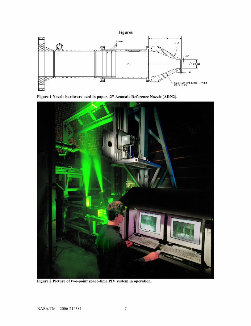
The nozzle being used in this test is one of a family of convergent nozzles, called the Acoustic Reference Nozzles (ARN), designed to be simple to characterize with similar dimensions such as inlet diameter (15.24mm), lip thickness (1.27mm), outside face angle (30° to jet axis), and parallel flow section at the exit (6.4mm). For this test, the ARN2, a 50.8mm or 2” diameter nozzle, was used (see Figure 1).

Datasets were acquired about five different axial reference locations in the Dj = 51mm jet: x1/Dj = 2, 6, 10, 16, and 22 for three different flow conditions given in Table 1. Given the many displacements used around each reference point the jet plume was fully covered by multiple datasets that could be averaged to provide measurements of single-point statistics such as mean and mean-square of velocity.

The flow conditions were chosen from a larger matrix of conditions being used to build up a jet aero/acoustic database and contain essentially two different velocities and static temperature ratios. Note that depending upon whether one specifies acoustic Mach number (Ma, jet exit velocity normalized by speed of sound of the ambient) or gas dynamic Mach number (M, jet exit velocity normalized by speed of sound in the jet), one can get a dramatically different jet! Of the seven flows measured, three will be analyzed in depth. Setpoint 7 is referred to as Ma=0.9, cold jet. Setpoint 46 has the same acoustic Mach number, but has been heated to roughly 2.7 times the ambient temperature, meaning that its gas dynamic Mach number is only 0.55. Setpoint 49 has a gas dynamic Mach number of 0.9, but an acoustic Mach number of 1.45, again at a static temperature ratio of 2.7. Here the flow is subsonic in that it is shock-free, but supersonic in that the convection speed is approaching the speed of sound in the ambient. These three cases bracket the basic flows faced in subsonic aircraft plumes.

Table 1 Definition of test conditions. The three setpoints in bold are analyzed in depth in this paper.

Set point Ma Tj/T∞ NPR M Witze

parameter

!

2" #$ # j

3 0.48 0.95 1.180 0.51 6.91 7 0.89 0.84 1.837 0.98 7.79 23 0.49 1.76 1.101 0.38 5.67 27 0.88 1.76 1.353 0.68 5.98 29 1.32 1.76 1.903 1.01 6.36 46 0.89 2.7 1.227 0.56 4.98 49 0.68 2.7 1.317 0.92 5.55

III. � Instrumentation Two PIV systems were used for this experimental effort, tied together via a triggering circuit with

variable time delay. Each PIV system consisted of a dual head Nd:YAG laser operating at 532 nm generating a 400 mJ/pulse light sheet containing the jet axis. Each laser was coordinated with a single 2000 by 2000 pixel dual-frame camera viewing the light sheet at right angles, one on each side of the light sheet. Image frame pairs were obtained by straddling adjacent frame boundaries. A PCI frame digitizer was used to acquire image data directly to disk in 200 image-pair sequences. Each camera viewed the same 170mm square field of view, centered on the jet axis, from a distance of 1.4m.

Velocity maps were computed from the image pairs using conventional multipass PIV algorithms with error detection based upon image correlation signal to noise ratio (NASA PIVPROC software). Final velocity maps had a spatial resolution of 0.02Dj. A minimal number of velocity maps (200) were acquired at each space-time separation to obtain rough estimates of the correlations. Based upon convergence of the statistics, the error in the final correlation data is estimated at ±5%.

More detail on the data acquisition aspects of this dataset can be found in Bridges & Wernet10. A photo of the two-point space-time PIV setup is given in Figure 2.

3NASA/TM—2006-214381

IV. Results

A. Single-point statistics Before delving into the details of two-point space-time correlations it is useful to better understand the

overall effect of adding heat to the jet. Figure 3 presents the mean velocity

!

U Uid and the mean-square of

velocity

!

uu Uid

2 for the three jet flows highlighted in Table 1. There is a clear decrease in the potential

core length as the jet is heated, either holding jet velocity constant (setpoint 46) or holding gas Mach number approximately constant (setpoint 49). There is also a small increase in turbulence level overall in the hot jets.

When comparing the potential core length of a jet, the Witze correlation lengthscale is a good way to collapse jets of many different speeds and temperatures. The centerline values from the mean and mean-square velocity fields of all the flows listed in Table 1 are extracted and plotted in Figure 4, first against actual axial distance and then against axial distance normalized by the Witze12 correlation parameter. The latter axial distance is specifically xw/Dj = (x/Dj) 2 κ (ρ∞/ρj)

0.5, where κ = 0.08 (1-0.16*Uid/c∞)–0.22, ρj is the density at the jet exit, ρ∞, and c∞ are the density and speed of sound in the ambient, and Uid is the ideally expanded jet velocity. In effect, xw/Dj is the predicted potential core length of the jet. This normalization not only collapses the end of the potential core fairly well, it does a fair job of collapsing the asymptotic decay region as well. Likewise, the centerline turbulence, given by the mean-square of axial velocity,

!

uu Uid

2 , collapses fairly well also. The scatter in peak mean-square velocity is roughly 0.003, 15% of the

peak, falling slightly outside the uncertainty of the measurement which has been determined from repeated runs and comparison with hotwire data. To isolate the impact of temperature on the turbulence, data for setpoints 7, 27, and 46, all at Ma = 0.9, have been isolated in Figure 5, where the difference in peak turbulence is seen to be a difference of roughly 10% in the mean-square. To put this in perspective, mean-square velocity, raised to the 7/2 power, will be proportional to acoustic source strength in cold jets. In this regard the 10% spread in variance corresponds to 1.3dB difference in noise, This is a small difference compared to the impact of heat on density for acoustic source strength.

Summarizing, it appears that temperature has little effect on peak turbulence levels for a given velocity (Ma) jet. Within a 10% uncertainty band, the jet mean and turbulence fields can be collapsed by normalizing for the potential core length and jet velocity.

A. Two-point statistics Moving on to the correlation data which figures prominently in most aeroacoustic theory, Figure 6 gives an example of the two-point space-time data acquired using the dual PIV system.

Correlation data has been acquired in three dimensions, axial and radial spatial separations

!

"1,"2 , and temporal separation

!

" . In the figure the correlation coefficient for the axial velocity is plotted against separation in non-dimensionalized axial, radial, and temporal separation at a point in the flow x/Dj = 6, y/Dj

= 0.5. The spatial separations are non-dimensionalized by jet diameter while the temporal separations are scaled by jet exit velocity and diameter. The peak of the correlation occurs at zero separation and extends on a ‘ridge’ which follows the local convection velocity. This convection velocity can be extracted from the space-time data for different regions of the jet to observe the impact of heat on this important parameter. This process is illustrated in Figure 7, where peaks are located in scans of Ruu at ξ2/Dj = 0 for various τ U/Dj. Numerical routines were developed which picked peaks of smoothed data to extract the convection velocity. Local peaks were found near these to extract the amplitude of Ruu for calculation of timescales.

The convection velocity obtained for the various jets as extracted along the centerline (Figure 8) and the lipline (Figure 9) of the nozzle are shown, plotted first against actual axial distance and then against axial distance normalized by the Witze correlation parameter. There is a fair amount of scatter in the convection velocity on the centerline near the nozzle because of the relatively small fluctuation levels, perhaps as much as ±0.1 in Uc/Uid. Elsewhere the uncertainty is closer to 0.05 based upon the quality of the fit of peaks to a line.

Even with this uncertainty a few trends are apparent. First, use of the Witze parameter to scale axial distance collapses the convection velocity data to a significant degree. Second, convection velocities on the centerline start at values around 0.7 within the potential core, but do not decay as a simple fraction of the centerline mean velocity. Instead, convection velocities collapse to the local mean velocity as the shear layer is reduced. Third, The convection velocity on the lipline is larger than the local mean, reaching a peak

4NASA/TM—2006-214381

difference near the end of the potential core before rather quickly collapsing back to the local mean velocity.

When trying to sort the impact of temperature on the convection velocity, trends are better observed by isolating a given Ma while varying temperature ratio. This is done in Figure 10 where convection velocity along the jet lipline is plotted against Xw/Dj. for Ma = 0.5 and Ma = 0.9. In both cases, adding heat seems to increase the convection velocity at the end of the potential core. Going the other way, Figure 11 presents the effect of Ma for a fixed temperature ratio. Here, the convection velocities do not depend upon Ma, except in the cold case where convection velocity is increased at all axial locations with increase in Ma.

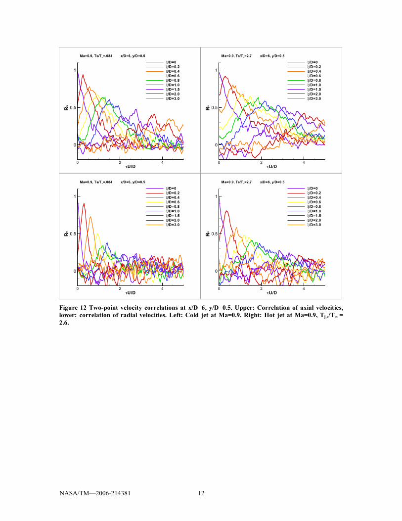
The data acquired by the dual-PIV system were obtained at lines of constant time delay, with high resolution in spatial separation, very unlike the way these correlations are usually measured with methods that acquire long time records at limited spatial points. If the data are resampled in temporal separation across lines of constant axial separation, the conventional view of the correlation function is extracted. Such extraction has been done for the two cases of hot and cold jets at constant jet velocity, shown in Figure 12. The reference point of this data is x/D=6, y/D=0.5. In these plots the temporal variation in correlation coefficient of the axial and radial components of velocity are shown for many spatial separations. Although the graphs seem very busy, and curves are not as smooth as presented by others using more averages of time-based instrumentation systems, the salient points are clear. The envelope of the peaks in correlation can be observed to decay in a convective frame of reference, allowing the temporal

correlation timescale

!

" 0 to be determined by fitting the peaks to an exponential function

!

e"# /# 0 .

Furthermore, by inspection, the general trends of adding heat to the jet can be discerned. The figures on the left side show the correlation of axial and radial velocity components from the cold jet case, while the figures on the right side show the same for the hot jet with the same exit velocity. While there are some differences between the two, they are not as dramatic as has been projected based upon previous density correlation methods.

Having extracted the correlation peaks in space-time, and determined the convective velocity and peak decay, the results for the timescale of the three jet flows are presented in Figure 13. In the figures, estimates of the timescale are given along the lipline of the jet. Data are plotted for jets with constant Ma = 0.9 and at constant static temperature ratio on the same plots. In one plot the axial distance is actual distance while in the other the axial distance has again been normalized by the Witze correlation parameter to remove the effect of differences in potential core length. Unlike in data presented above, the Witze scaling does not help collapse the data, especially in the region of the jet where most jet noise is produced. Perhaps because the timescale of the jet is more dependent upon the shear layer thickness rather than the potential core length, Witze scaling is not appropriate for timescales.

What is clear from Figure 13 is that the cold and hot jets have very similar timescales within the first 10 jet diameters, where most of the turbulent kinetic energy is located. In the asymptotic decay region, arguably where the very lowest frequencies of noise are produced, they differ substantially, with the heated Ma=0.9 jet having timescales as much as twice that of the cold jet. This should be put in perspective by noting that most jet noise spectra is presented on a log-frequency scale, meaning that even this difference of a factor of two in timescale may not result in a major change to the expected spectral shape. It is a trend in the right direction, however.

Jet noise theory requires consideration of more than just a single component of turbulence, and Figure 14 shows how axial and radial components of velocity decorrelate as they convect downstream. In this figure the timescale computed using the axial velocity component is plotted on the left axis while the timescale computed using the radial velocity component is plotted on the left axis. In the theory of homogeneous turbulence the correlation lengths produced by velocity components parallel and normal to the separation differ by a factor of 2. It is interesting then to note that this is roughly the ratio observed in the temporal decay rates in the jet, relatively independent of temperature.

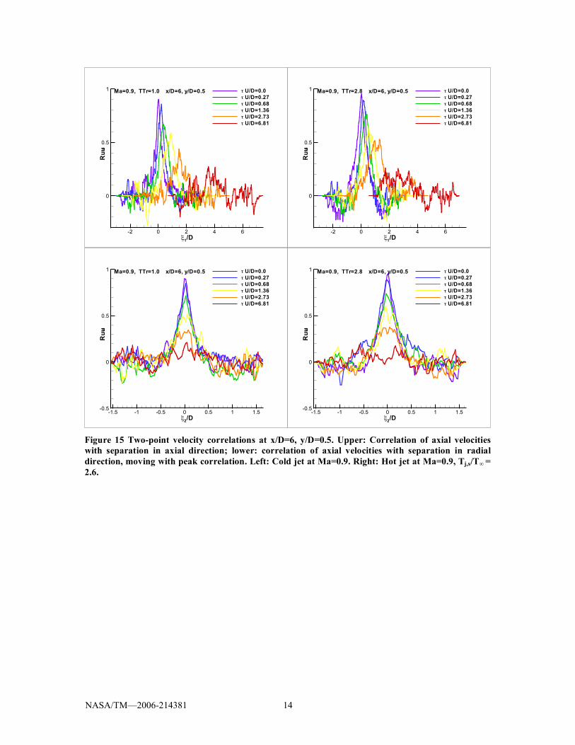
While most previous measurements of velocity correlation have been presented in the temporal domain, it is interesting to consider the correlation as a function of spatial separation. Figure 15 presents this view for the same location in the jet, x/D=6, y/D=0.5 as was shown before for temporal separations. In this upper half of this figure the correlation of axial velocity with axial separation is shown for the cold (left) and hot (right) jets, again noting that the decay is not that different for the two. What may be of more importance is the substantially larger negative swings in the correlation curves of the hot jet. When transformed to spectra, these negative loops create more low frequency content. This might be critical to the proper modeling of the low frequency noise sources in the hot jet. In the lower half of the figure the correlation of

5NASA/TM—2006-214381

axial velocity over radial separation is shown. The hot jet has a slightly wider region of correlation radially, an aspect which may be explained by the faster axial development. This, too, may be important for including in models of the acoustic source.

From plots such as those in Figure 15, correlation curves are integrated to produce estimates for lengthscales. As with all experimental measurements of lengthscale, the fluctuation in the correlation coefficient around zero adds uncertainty to the measurement. Two different methods were used in estimating lengthscale: first a simple direct integration with a tapered weighting of the tails away from zero, and second a fitting of an appropriate turbulence model to the correlation and determination of the lengthscale from the fitted coefficients. The good news was that both methods were consistent and for simplicity only the direct integration result is shown here.

Figure 17 shows the lengthscales estimated for cold and hot jet flows as a function of downstream location, integrating the correlation of axial velocity component u separated in axial direction over x (Luux) and the correlation of radial velocity component v separated in axial direction over x (Lvvx). Figure 17 contains the same information for separations in radial direction y, (Luuy, Lvvy). . These lengthscales were measured along the jet lipline y/D = 0.5 are shown plotted against actual axial location (right) and against Witze-normalized distance (left). In homogenous turbulence Luux = Lvvy, etc., but clearly this is not homogeneous turbulence. While the uncertainty in the measurement of lengthscale is significant, perhaps ±0.1Dj, it does appear that the Witze normalization does help collapse the data for the Luux and Lvvx lengthscales. It is not as clear whether there is any improvement in the radial separation lengthscales. In spite of the experimental uncertainty, the main point for this paper is that adding heat to the jet does not change the lengthscales by more than 50% in regions of the jet that produce significant jet noise.

V. � Conclusions Measurements of space-time correlation of velocity have been presented in both cold and hot jets,

focusing on acoustic Mach number Ma=0.9. The single-point statistics showed that with the addition of heat the potential core of the jet shrank, but the turbulence intensity increased only slightly. While the cold and hot jets had potential core lengths which varied by 50%, the Witze correlating parameter collapses the potential cores of all the jets. Using this normalization, centerline mean velocity and turbulence were shown to collapse onto one curve for all jets. The two-point statistics show that convection velocity of the turbulence is slightly affected by heating, becoming 10%–20% higher at the end of the potential core. By twice the potential core length, convection velocity on the lipline is the same as the local mean velocity for all jets. Velocity correlations are slightly different in character with the addition of heat, signaling a slight change in the turbulence spectrum with heating, but the overall measures of timescale are not strongly altered until long after the end of the potential core where the hot jet has a substantially larger timescale. Similarly, measures of the lengthscale show a slight lengthening of the turbulence with heating, perhaps 10-20%. Overall, it is observed that the effect of heat on the jet is relatively benign once changes in the potential core length have been accounted for.

6NASA/TM—2006-214381

Figures

Figure 1 Nozzle hardware used in paper--2" Acoustic Reference Nozzle (ARN2).

Figure 2 Picture of two-point space-time PIV system in operation.

7NASA/TM—2006-214381

x/Dj

y/Dj

0 2 4 6 8 10-2

-1

0

1

2 U/Uid: 0.1 0.3 0.5 0.7 0.9

T1 ARN2 SP007

x/Dj

y/Dj

0 2 4 6 8 10-2

-1

0

1

2 uu/Uid^2: 0 0.01 0.02 0.03

T1 ARN2 SP007

x/Dj

y/Dj

0 2 4 6 8 10-2

-1

0

1

2 U/Uid: 0.1 0.3 0.5 0.7 0.9

T1 ARN2 SP046

x/Dj

y/Dj

0 2 4 6 8 10-2

-1

0

1

2 uu/Uid^2: 0 0.01 0.02 0.03

T1 ARN2 SP046

x/Dj

y/Dj

0 2 4 6 8 10-2

-1

0

1

2 U/Uid: 0.1 0.3 0.5 0.7 0.9

T1 ARN2 SP049

x/Dj

y/Dj

0 2 4 6 8 10-2

-1

0

1

2 uu/Uid^2: 0 0.01 0.02 0.03

T1 ARN2 SP049

Figure 3 Mean and variance of cold and hot jets. Three jets: Ma=0.9, Tj,s/T∞ = 0.84 (top); Ma=0.9, Tj,s/T∞ = 2.7 (middle); Ma=1.45, Tj,s/T∞ = 2.7 (bottom).

x/Dj

U/Uid

uu/Uid2

0 5 10 15 20 25

0

0.2

0.4

0.6

0.8

1

0

0.01

0.02

0.03

0.04

0.05

0.06

0.07

3

7

23

27

29

46

49

y/D = 0

Setpoint

xw/Dj

U/Uid

uu/Uid2

0 1 2 3 4 5

0

0.2

0.4

0.6

0.8

1

0

0.01

0.02

0.03

0.04

0.05

0.06

0.07

3

7

23

27

29

46

49

y/D = 0

Setpoint

Figure 4 Mean and mean-square of axial velocity along centerline for hot and cold subsonic jets, plotted against actual distance (left), and normalized by Witze correlation parameter (right). See Table 1 for definitions of setpoints.

8NASA/TM—2006-214381

x/Dj

U/Uid

uu/Uid2

0 5 10 15 20 25

0

0.2

0.4

0.6

0.8

1

0

0.01

0.02

0.03

0.04

0.05

0.06

0.07

7

27

46

y/D = 0

Setpoint

xw/Dj

U/Uid

uu/Uid2

0 1 2 3 4 5

0

0.2

0.4

0.6

0.8

1

0

0.01

0.02

0.03

0.04

0.05

0.06

0.07

7

27

46

y/D = 0

Setpoint

Figure 5 Mean and mean-square of axial velocity along centerline for Ma=0.9 jets at different temperature ratios, plotted against actual distance (left) and normalized by Witze correlation parameter (right). Setpoints 7, 27, and 46 have static temperature ratios of 0.84, 1.76, and 2.7, respectively.

Figure 6 Example of velocity correlation data in ξ1, τ plane. Ma=0.9, Tj,s/T∞ = 0.84.

9NASA/TM—2006-214381

!1/Dj

"Uid/Dj

0 2 4

0

1

2

3

4

ARN2 SP7x/D=6, y/D=0.5Ruu

!1/Dj = 1.8

"Uid/Dj = 2.73!1/("Uid) = 0.65

!1/Dj = 0.23

"Uid/Dj = 0.273!1/("Uid) = 0.84

!1/Dj = 0.483

"Uid/Dj = 0.683!1/("Uid) = 0.71

!1/Dj = 0.93

"Uid/Dj = 1.364!1/("Uid) = 0.70

Figure 7 Finding convection velocity from space-time correlations of axial velocity. This example taken from setpoint 7, x/Dj = 6, y/Dj = 0.5. Here, average convection velocity determined to be 0.7.

x/Dj

Uc/Uid

0 5 10 15 20 250

0.2

0.4

0.6

0.8

1

0.48, 0.96

0.89, 0.87

0.49, 1.76

0.89, 1.74

1.32, 1.74

0.89, 2.65

1.46, 2.55

Ma, Ts/T!

y/Dj = 0.0

Xw/Dj

Uc/Uid

U/Uid

0 1 2 3 4 50

0.2

0.4

0.6

0.8

1

0

0.2

0.4

0.6

0.8

1

0.48, 0.96

0.89, 0.87

0.49, 1.76

0.89, 1.74

1.32, 1.74

0.89, 2.65

1.46, 2.55

1.46, 2.70

Ma, Ts/T!

y/Dj = 0.0

Figure 8 Convective velocities for cold and hot jets, along centerline, plotted against actual distance (left) and normalized by Witze correlation parameter (right). Data obtained by tracking peak in space-time correlation of axial velocities. Typical centerline mean velocity plotted on Witze-scaled plot for reference.

10NASA/TM—2006-214381

x/Dj

Uc/Uid

0 5 10 15 20 250

0.2

0.4

0.6

0.8

1

0.48, 0.96

0.89, 0.87

0.49, 1.76

0.89, 1.74

1.32, 1.74

0.89, 2.65

1.46, 2.55

Ma, Ts/T!

y/Dj = 0.5

Xw/Dj

Uc/Uid

U/Uid

0 1 2 3 4 50

0.2

0.4

0.6

0.8

1

0

0.2

0.4

0.6

0.8

1

0.48, 0.96

0.89, 0.87

0.49, 1.76

0.89, 1.74

1.32, 1.74

0.89, 2.65

1.46, 2.55

1.48, 2.6

Ma, Ts/T!

y/Dj = 0.5

Figure 9 Convective velocities for cold and hot jets, along lipline (y/Dj = 0.5), plotted against actual distance (left) and normalized by Witze correlation parameter (right). Data obtained by tracking peak in space-time correlation of axial velocities. Typical mean velocity at this radius plotted on Witze-scaled plot for reference.

Xw/Dj

Uc/Uid

0 1 2 3 4 50

0.2

0.4

0.6

0.8

1

0.48, 0.96

0.49, 1.76

Ma, Ts/T!

y/Dj = 0.5

Xw/Dj

Uc/Uid

0 1 2 3 4 50

0.2

0.4

0.6

0.8

1

0.89, 0.87

0.89, 1.74

0.89, 2.65

Ma, Ts/T!

y/Dj = 0.5

Figure 10 Convective velocities for Ma = 0.5 (left) and Ma = 0.9 (right) jets at different temperatures, measured along lipline (y/Dj = 0.5), plotted against distance normalized by Witze correlation parameter.

Xw/Dj

Uc/Uid

0 1 2 3 4 50

0.2

0.4

0.6

0.8

1

0.48, 0.96

0.89, 0.87

Ma, Ts/T!

y/Dj = 0.5

Xw/Dj

Uc/Uid

0 1 2 3 4 50

0.2

0.4

0.6

0.8

1

0.49, 1.76

0.89, 1.74

Ma, Ts/T!

y/Dj = 0.5

Xw/Dj

Uc/Uid

0 1 2 3 4 50

0.2

0.4

0.6

0.8

1

0.89, 2.65

1.46, 2.55

Ma, Ts/T!

y/Dj = 0.5

Figure 11 Convective velocities for jets at different Ma, same temperature ratios, measured along lipline (y/Dj = 0.5), plotted against distance normalized by Witze correlation parameter.

11NASA/TM—2006-214381

!U/D

Ruu

0 2 4

0

0.5

1

"/D=0

"/D=0.2

"/D=0.4

"/D=0.6

"/D=0.8

"/D=1.0

"/D=1.5

"/D=2.0

"/D=3.0

Ma=0.9, Ts/T#=.084 x/D=6, y/D=0.5

!U/D

Ruu

0 2 4

0

0.5

1

"/D=0

"/D=0.2

"/D=0.4

"/D=0.6

"/D=0.8

"/D=1.0

"/D=1.5

"/D=2.0

"/D=3.0

Ma=0.9, Ts/T#=2.7 x/D=6, y/D=0.5

!U/D

Rvv

0 2 4

0

0.5

1

"/D=0

"/D=0.2

"/D=0.4

"/D=0.6

"/D=0.8

"/D=1.0

"/D=1.5

"/D=2.0

"/D=3.0

Ma=0.9, Ts/T#=.084 x/D=6, y/D=0.5

!U/D

Rvv

0 2 4

0

0.5

1

"/D=0

"/D=0.2

"/D=0.4

"/D=0.6

"/D=0.8

"/D=1.0

"/D=1.5

"/D=2.0

"/D=3.0

Ma=0.9, Ts/T#=2.7 x/D=6, y/D=0.5

Figure 12 Two-point velocity correlations at x/D=6, y/D=0.5. Upper: Correlation of axial velocities, lower: correlation of radial velocities. Left: Cold jet at Ma=0.9. Right: Hot jet at Ma=0.9, Tj,s/T∞ = 2.6.

12NASA/TM—2006-214381

x/Dj

! uUid/Dj

0 5 10 15 20 250

5

10

15

20

0.89, 0.87, !uUid/Dj

0.89, 2.7, !uUid/Dj

1.46, 2.6, !uUid/Dj

Ma, Ts/T"

y/D = 0.5

Xw/Dj

! uUid/Dj

0 1 2 3 4 50

5

10

15

20

0.89, 0.87, !uUid/Dj

0.89, 2.7, !uUid/Dj

1.46, 2.6, !uUid/Dj

Ma, Ts/T"

y/D = 0.5

Figure 13 Timescales of cold and hot jets derived from envelope of correlation peaks in space-time. Correlation of axial velocities. Normal scaling of axial location on left, Witze scaling of axial location on right.

x/Dj

! uUid/Dj

! vUid/Dj

0 5 10 15 20 250

5

10

15

20

0

2

4

6

8

10

0.89, 0.87, !uUid/Dj

0.89, 2.7, !uUid/Dj

1.46, 2.6, !uUid/Dj

0.89, 0.87, !vUid/Dj

0.89, 2.7, !vUid/Dj

1.46, 2.6, !vUid/Dj

Ma, Ts/T"

y/D = 0.5

Figure 14 Timescales of cold and hot jets derived from envelope of correlation peaks in space-time. Correlation of axial velocities (left axis); correlation of radial velocities (right axis). Note the change in scales for the different components.

13NASA/TM—2006-214381

!1/D

Ruun

-2 0 2 4 6

0

0.5

1 " U/D=0.0

" U/D=0.27

" U/D=0.68

" U/D=1.36

" U/D=2.73

" U/D=6.81

Ma=0.9, TTr=1.0 x/D=6, y/D=0.5

!1/D

Ruun

-2 0 2 4 6

0

0.5

1 " U/D=0.0

" U/D=0.27

" U/D=0.68

" U/D=1.36

" U/D=2.73

" U/D=6.81

Ma=0.9, TTr=2.8 x/D=6, y/D=0.5

!2/D

Ruun

-1.5 -1 -0.5 0 0.5 1 1.5-0.5

0

0.5

1 " U/D=0.0

" U/D=0.27

" U/D=0.68

" U/D=1.36

" U/D=2.73

" U/D=6.81

Ma=0.9, TTr=1.0 x/D=6, y/D=0.5

!2/D

Ruun

-1.5 -1 -0.5 0 0.5 1 1.5-0.5

0

0.5

1 " U/D=0.0

" U/D=0.27

" U/D=0.68

" U/D=1.36

" U/D=2.73

" U/D=6.81

Ma=0.9, TTr=2.8 x/D=6, y/D=0.5

Figure 15 Two-point velocity correlations at x/D=6, y/D=0.5. Upper: Correlation of axial velocities with separation in axial direction; lower: correlation of axial velocities with separation in radial direction, moving with peak correlation. Left: Cold jet at Ma=0.9. Right: Hot jet at Ma=0.9, Tj,s/T∞ = 2.6.

14NASA/TM—2006-214381

x/Dj

Luux/Dj

Lvvx/Dj

0 5 10 15 20 250

0.2

0.4

0.6

0.8

1

0

0.2

0.4

0.6

0.8

1

0.89, 0.84, Luux/Dj

0.89, 2.7, Luux/Dj

1.48, 2.6, Luux/Dj

0.89, 0.84, Lvvx/Dj

0.89, 2.7, Lvvx/Dj

1.48, 2.6, Lvvx/Dj

Ma, Ts/T!

y/D = 0.5

Xw/Dj

Luux/Dj

Lvvx/Dj

0 1 2 3 4 50

0.2

0.4

0.6

0.8

1

0

0.2

0.4

0.6

0.8

1

0.89, 0.84, Luux/Dj

0.89, 2.7, Luux/Dj

1.48, 2.6, Luux/Dj

0.89, 0.84, Lvvx/Dj

0.89, 2.7, Lvvx/Dj

1.48, 2.6, Lvvx/Dj

Ma, Ts/T!

y/D = 0.5

Figure 16 Lengthscales for cold and hot jets, computed over axial displacements of axial (Luux) and radial (Lvvx) velocity components, for reference locations on the lipline of the jet. Left: actual axial location Right: axial location normalized by Witze correlation parameter.

x/Dj

Luuy/Dj

Lvvy/Dj

0 5 10 15 20 250

0.2

0.4

0.6

0.8

1

0

0.2

0.4

0.6

0.8

1

0.89, 0.84, Luuy/Dj

0.89, 2.7, Luuy/Dj

1.48, 2.6, Luuy/Dj

0.89, 0.84, Lvvy/Dj

0.89, 2.7, Lvvy/Dj

1.48, 2.6, Lvvy/Dj

Ma, Ts/T!

y/D = 0.5

Xw/Dj

Luuy/Dj

Lvvy/Dj

0 1 2 3 4 50

0.2

0.4

0.6

0.8

1

0

0.2

0.4

0.6

0.8

1

0.89, 0.84, Luuy/Dj

0.89, 2.7, Luuy/Dj

1.48, 2.6, Luuy/Dj

0.89, 0.84, Lvvy/Dj

0.89, 2.7, Lvvy/Dj

1.48, 2.6, Lvvy/Dj

Ma, Ts/T!

y/D = 0.5

Figure 17 Lengthscales for cold and hot jets, computed over radial displacements of axial (Luuy) and radial (Lvvy) velocity components, for reference locations on the lipline of the jet. Left: actual axial location Right: axial location normalized by Witze correlation parameter.

VI. � References 1 Laurence, J.R. 1956, “Intensity, scale, and spectra of turbulence in mixing region of free subsonic jet, “NACA Report 1292. 2 Bradshaw, P., Ferriss, D.H., Johnson, R.F. 1963, “Turbulence in the noise-producing region of a circular jet,” J Fluid Mech 19, 591-625.

3 Davies, P.O.A.L., Fisher, K.J., and Barratt, M.J. 1963,“The characteristics of turbulence in the mixing region of a round jet,” J Fluid Mech 15, 337-367.

4 Chu, W.T.1966, “Turbulence measurements relevant to jet noise,” Univ. Toronto Institute for Aerospace Studies UTIAS Report 119.

5 Doty, M. J., and McLaughlin, D. K., “Two-Point Correlations of Density Gradient Fluctuations in High Speed Jets Using Optical Deflectometry,” AIAA Paper 2002-0367, Jan. 2002.

6 Panda, J., Seasholtz, R. G., and Elam, K. A., “Further Progress in Noise Source Identification in High Speed Jets via Causality Principle,” AIAA Paper 2003-3126, May 2003

15NASA/TM—2006-214381

7 Tam, C.K.W., Pastouchenko, N.N., And Viswanathan, K., “Fine-scale turbulence noise from hot jets,” AIAA

Journal, Vol 43 (8), 2005, pp. 1675-1683. 8 Tam, C. K. W., and Ganesan, A., “A Modified k–ε Turbulence Model for Calculating the Mean Flow and Noise

of Hot Jets,” AIAA Journal,Vol. 42, No. 1, 2004, pp. 26–34. 9 Viswanathan, K., “Aeroacoustics of Hot Jets,” Journal of Fluid Mechanics, 516, 2004, pp. 39–82. 10 Bridges, J. & Wernet, M.P. “Measurements of the aeroacoustic sound source in hot jets,” AIAA 2003-3130

(2003). 11 Bridges, J. & Brown, C.A., “Validation of the Small Hot Jet Acoustic Rig for Jet Noise Research,” AIAA Paper

2005-2846, May 2005. 12 Witze, P.O., 1974, “Centerline velocity decay of compressible free jets,” AIAA J 12(4), 417-418.

16NASA/TM—2006-214381

This publication is available from the NASA Center for AeroSpace Information, 301–621–0390.

REPORT DOCUMENTATION PAGE

2. REPORT DATE

19. SECURITY CLASSIFICATION OF ABSTRACT

18. SECURITY CLASSIFICATION OF THIS PAGE

Public reporting burden for this collection of information is estimated to average 1 hour per response, including the time for reviewing instructions, searching existing data sources,gathering and maintaining the data needed, and completing and reviewing the collection of information. Send comments regarding this burden estimate or any other aspect of thiscollection of information, including suggestions for reducing this burden, to Washington Headquarters Services, Directorate for Information Operations and Reports, 1215 JeffersonDavis Highway, Suite 1204, Arlington, VA 22202-4302, and to the Office of Management and Budget, Paperwork Reduction Project (0704-0188), Washington, DC 20503.

NSN 7540-01-280-5500 Standard Form 298 (Rev. 2-89)Prescribed by ANSI Std. Z39-18298-102

Form Approved

OMB No. 0704-0188

12b. DISTRIBUTION CODE

8. PERFORMING ORGANIZATION REPORT NUMBER

5. FUNDING NUMBERS

3. REPORT TYPE AND DATES COVERED

4. TITLE AND SUBTITLE

6. AUTHOR(S)

7. PERFORMING ORGANIZATION NAME(S) AND ADDRESS(ES)

11. SUPPLEMENTARY NOTES

12a. DISTRIBUTION/AVAILABILITY STATEMENT

13. ABSTRACT (Maximum 200 words)

14. SUBJECT TERMS

17. SECURITY CLASSIFICATION OF REPORT

16. PRICE CODE

15. NUMBER OF PAGES

20. LIMITATION OF ABSTRACT

Unclassified Unclassified

Technical Memorandum

Unclassified

National Aeronautics and Space AdministrationJohn H. Glenn Research Center at Lewis FieldCleveland, Ohio 44135–3191

1. AGENCY USE ONLY (Leave blank)

10. SPONSORING/MONITORING AGENCY REPORT NUMBER

9. SPONSORING/MONITORING AGENCY NAME(S) AND ADDRESS(ES)

National Aeronautics and Space AdministrationWashington, DC 20546–0001

Available electronically at http://gltrs.grc.nasa.gov

September 2006

NASA TM—2006-214381AIAA–2006–2534

E–15659

WBS–22–781–30–63

22

Effect of Heat on Space-Time Correlations in Jets

James Bridges

Jet flow; Particle image velocimetry; Turbulence; Velocity correlation;Turbulent kinetic energy; Aeroacoustics

Unclassified -UnlimitedSubject Categories: 7, 9, and 34

Prepared for the 12th Aeroacoustics Conference cosponsored by American Institute of Aeronautics and Astronautics andConfederation of European Aerospace Societies, May 8–10, 2006. Responsible person, James Bridges, organization codeRTA, 216–433–2693.

Measurements of space-time correlations of velocity, acquired in jets from acoustic Mach number 0.5 to 1.5 and statictemperature ratios up to 2.7 are presented and analyzed. Previous reports of these experiments concentrated on theexperimental technique and on validating the data. In the present paper the dataset is analyzed to address the question ofhow space-time correlations of velocity are different in cold and hot jets. The analysis shows that turbulent kinetic energyintensities, lengthscales, and timescales are impacted by the addition of heat, but by relatively small amounts. This contra-dicts the models and assumptions of recent aeroacoustic theory trying to predict the noise of hot jets. Once the change injet potential core length has been factored out, most one- and two-point statistics collapse for all hot and cold jets.