Page 1
EFFECT OF JOINT FLEXIBILITY ON THE NONLINEAR STATIC
AND DYNAMIC BEHAVIOUR OF OFFSHORE JACKET
PLATFORMS
HAMIDREZA GOLABI
DISSERTATION SUBMITTED IN FULFILMENT OF THE
REQUIREMENTS FOR THE DEGREE OF MASTER OF SCIENCE
INSTITUTE OF GRADUATE STUDIES
UNIVERSITY OF MALAYA
KUALA LUMPUR
2015
Page 2
i
UNIVERSITI MALAYA
PERAKUAN KEASLIAN PENULISAN
Nama: HAMIDREZA GOLABI
No. Pendaftaran/Matrik: KGA080063
Nama Ijazah: MASTER OF ENGINEERING SCIENCE
Tajuk Kertas Projek/Laporan Penyelidikan/Disertasi/Tesis (“Hasil Kerja ini”):
EFFECT OF JOINT FLEXIBILITY ON THE NONLINEAR STATIC AND
DYNAMIC BEHAVIOUR OF OFFSHORE JACKET PLATFORMS
Bidang Penyelidikan: STRUCTURAL ENGINEERING AND MATERIALS
Saya dengan sesungguhnya dan sebenarnya mengaku bahawa:
(1) Saya adalah satu-satunya pengarang/penulis Hasil Kerja ini;
(2) Hasil Kerja ini adalah asli;
(3) Apa-apa penggunaan mana-mana hasil kerja yang mengandungi hakcipta telah
dilakukan secara urusan yang wajar dan bagi maksud yang dibenarkan dan apa-
apa petikan, ekstrak, rujukan atau pengeluaran semula daripada atau kepada
mana-mana hasil kerja yang mengandungi hakcipta telah dinyatakan dengan
sejelasnya dan secukupnya dan satu pengiktirafan tajuk hasil kerja tersebut dan
pengarang/penulisnya telah dilakukan di dalam Hasil Kerja ini;
(4) Saya tidak mempunyai apa-apa pengetahuan sebenar atau patut semunasabahnya
tahu bahawa penghasilan Hasil Kerja ini melanggar suatu hakcipta hasil kerja
yang lain;
(5) Saya dengan ini menyerahkan kesemua dan tiap-tiap hak yang terkandung di
dalam hakcipta Hasil Kerja ini kepada Universiti Malaya (“UM”) yang
seterusnya mula dari sekarang adalah tuan punya kepada hakcipta di dalam Hasil
Kerja ini dan apa-apa pengeluaran semula atau penggunaan dalam apa jua
bentuk atau dengan apa juga cara sekalipun adalah dilarang tanpa terlebih
dahulu mendapat kebenaran bertulis dari UM;
(6) Saya sedar sepenuhnya sekiranya dalam masa penghasilan Hasil Kerja ini saya
telah melanggar suatu hakcipta hasil kerja yang lain sama ada dengan niat atau
sebaliknya, saya boleh dikenakan tindakan undang-undang atau apa-apa
tindakan lain sebagaimana yang diputuskan oleh UM.
Tandatangan Calon Tarikh
Diperbuat dan sesungguhnya diakui di hadapan,
Tandatangan Saksi Tarikh
Nama:
Jawatan:
Page 3
ii
UNIVERSITI MALAYA
ORIGINAL LITERARY WORK DECLARATION
Name of Candidate: HAMIDREZA GOLABI
Registration/Matric No: KGA080063
Name of Degree: MASTER OF ENGINEERING SCIENCE
Title of Project Paper/Research Report/Dissertation/Thesis (“this Work”):
EFFECT OF JOINT FLEXIBILITY ON THE NONLINEAR STATIC AND
DYNAMIC BEHAVIOUR OF OFFSHORE JACKET PLATFORMS
Field of Study: STRUCTURAL ENGINEERING AND MATERIALS
I do solemnly and sincerely declare that:
(1) I am the sole author/writer of this Work;
(2) This Work is original;
(3) Any use of any work in which copyright exists was done by way of fair dealing
and for permitted purposes and any excerpt or extract from, or reference to or
reproduction of any copyright work has been disclosed expressly and
sufficiently and the title of the Work and its authorship have been acknowledged
in this Work;
(4) I do not have any actual knowledge nor do I ought reasonably to know that the
making of this work constitutes an infringement of any copyright work;
(5) I hereby assign all and every rights in the copyright to this Work to the
University of Malaya (“UM”), who henceforth shall be owner of the copyright
in this Work and that any reproduction or use in any form or by any means
whatsoever is prohibited without the written consent of UM having been first
had and obtained;
(6) I am fully aware that if in the course of making this Work I have infringed any
copyright whether intentionally or otherwise, I may be subject to legal action or
any other action as may be determined by UM.
Candidate’s Signature Date
Subscribed and solemnly declared before,
Witness’s Signature Date
Name:
Designation:
Page 4
iii
ABSTRACT
Offshore steel jacket structures consist primarily of tubular members and associated
joints. Tubular members have been widely used due to their excellent properties in
respect of resistance in compression, tension, bending and torsion forces. In computer
analysis, connections between the elements are assumed to be rigid, which means that
there would be no axial rotational or deflection at the end of the secondary member
against the main member’s axis. Nevertheless, the tubular joints have a remarkable
amount of flexibility in the elasto-plastic range. Designing these structures based on
realistic conditions is important due to the high costs of design and construction. Several
studies based on numerical and experimental work have been done on tubular joints in
2-Dimensional states. In this study, finite element (FE) modelling of tubular
connections is carried out in 3-Dimensions, to account for the actual platform
performance.
In this study a 3-D model of a fixed steel platform existing in the Persian Gulf has been
modelled using a nonlinear finite element program. The joints and platform members
are modelled using a SHELL element and PIPE element, respectively, through ANSYS
software. Moreover, to investigate the effect of joint flexibility on these models, the
analysis of rigid and flexible models of the platform and comparison of their static and
dynamic behaviours are presented. In addition, push-over analyses were carried out for
several joints with and without Joint-cans and also a comparison of M curves in
these two conditions is reported.
The result of the non-linear static analysis shows that the static response of the structure
changed considerably with respect to the joints’ flexibility in the nonlinear range. The
modal features of the structure with flexible joints have significant differences
Page 5
iv
compared to the rigid joints structure. In addition, performing the dynamic time-history
analysis and investigating the exact effect of flexibility based on the flexible model
shows that base shear values are reduced by about 30% compared to the rigid model. It
is proven that local joint restraint has a considerable effect on the nonlinear static and
dynamic behaviour of offshore structures.
Page 6
v
ABSTRAK
Struktur keluli untuk pelantar luar pesisir terdiri daripada anggota keratan tiub dan
sambungan. Anggota keratan tiub telah digunakan secara meluas kerana ciri-ciri yang
cemerlang seperti rintangan dalam mampatan, ketegangan, daya lenturan dan kilasan.
Dalam analisis komputer, kebiasaannya sambungan di antara elemen diandaikan sebagai
tegar, iaitu tidak akan ada putaran paksi atau pesongan pada hujung anggota sekunder
terhadap paksi anggota utama. Walau bagaimanapun, sambungan tiub mempunyai
fleksibiliti yang luar biasa dalam julat elasto-plastik. Merekabentuk struktur ini
berasaskan kepada keadaan yang realistik adalah penting kerana kos yang tinggi bagi
rekabentuk dan pembinaan. Beberapa kajian yang berdasarkan kajian berangka dan
eksperimen telah dilakukan pada sambungan tiub dalam 2-dimensi. Dalam kajian ini,
kaedah unsur terhingga (FE) bagi sambungan tiub dijalankan dalam 3-dimensi, bagi
mengambil kira prestasi platform yang sebenar.
Didalam kajian ini sebuah model 3-D telah di bangunkan bagi pelantar keluli tegar yang
telah sedia ada di Teluk Parsi menggunakan analisis tak terhingga tak linear.
Sambungan dan anggota platform dimodelkan oleh unsur SHELL dan elemen PAIP
masing-masing melalui perisian ANSYS. Selain itu, untuk menyiasat kesan fleksibiliti
sendi pada model ini, analisis model tegar dan fleksibel bagi platform dan perbandingan
tingkah laku mereka secara statik dan dinamik dibentangkan. Di samping itu, analisis
push-over telah dijalankan bagi beberapa untuk sendi dengan dan tanpa ‘joint-can’ dan
juga perbandingan lengkung M dalam kedua-dua keadaan dilaporkan.
Hasil bagi analisis statik tak linear menunjukkan bahawa sambutan statik struktur jauh
berubah disebabkan oleh kesan fleksibiliti sendi dalam julat tak linear. Ciri-ciri ragaman
struktur dengan sendi fleksibel mempunyai perbezaan yang signifikan berbanding
dengan sendi struktur tegar. Sebagai tambahan, analisis dinamik ‘time-history’ dan
Page 7
vi
kajian ke atas kesan fleksibiliti sendi menunjukkan bahawa nilai ricih asas bagi model
fleksibel berkurangan kira-kira 30% berbanding dengan model tegar. Ia membuktikan
bahawa kekangan pada sendi tempatan mempunyai kesan yang besar ke atas tingkah
laku statik dan dinamik tak linear bagi struktur luar pesisir.
Page 8
vii
ACKNOWLEDGEMENTS
In the name of Allah, most gracious, most merciful, all praise and thanks are due to
Allah, and peace and blessings be upon His Messenger and relations.
Foremost, I would like to express my sincere gratitude to my advisors, Dr. Zainah
Ibrahim and Dr. Norhafizah Ramli@Sulong, for their continuous support during my
study and research, for their patience, motivation, enthusiasm, and immense knowledge.
Their guidance helped me throughout the time of the research and the writing of this
thesis. I could not have imagined having better advisors and mentors for my study.
Besides my advisors, I would like to thank my parents for supporting me spiritually
throughout my life.
Page 9
viii
CONTENTS
ABSTRACT III
ABSTRAK V
ACKNOWLEDGEMENTS VII
LIST OF FIGURES XI
LIST OF TABLES XV
LIST OF SYMBOLS XVI
LIST OF ABBREVIATIONS XVIII
1.0 INTRODUCTION 1
1.1 Introduction 1
1.2 Problem Statement 3
1.3 Objectives 3
1.4 Scope of Work 4
1.5 The Organisation of The Thesis 5
2.0 LITERATURE REVIEW 6
2.1 Introduction 6
2.2 Fixed Platforms 7
2.3 Selecting an Appropriate Platform to be Installed in the Persian Gulf 12
2.4 Tubular Elements 13
2.5 Tubular Joint Failure 18
2.6 Codes on Ultimate Resistance and Designing Tubular Joints 23
2.6.1 The API Code on Tubular Joints 23
2.6.2 Changes in API (2007) 27
2.7 Flexibility of Tubular Joints 29
2.7.1 Analytical Methods 30
2.7.2 Experimental and Semi-Experimental Methods 34
2.7.2.1 Experimental Methods 34
2.7.2.2 Semi-Experimental Methods 37
2.7.3 Numerical Methods 42
2.8 Joint Flexibility Models Based on Finite Element Methods 47
2.8.1 Bouwkamp Model 49
Page 10
ix
2.8.2 UEG Report, Node Flexibility and its Effects on |Jacket Structures 51
2.8.3 Chen Model 57
2.8.4 Souissi Model 59
2.8.5 Recho Model 60
2.8.6 Elnashai Model 62
2.8.7 Mirtaheri Model 68
3.0 DEVELOPMENT OF FINITE ELEMENT MODELS 71
3.1 Introduction 71
3.2 Finite Element Method 71
3.2.1 3-D Isoperimetric Finite Element 72
3.2.2 The Inelastic Analysis of Finite Element 73
3.3 Elements Used in modelling 74
3.3.1 PIPE 20 Element 74
3.3.2 SHELL 43 Element 75
3.3.3 MASS21 Element 76
3.4 Material Behaviour Model 77
3.4.1 Von-Mises Criterion 78
3.4.2 Steel Profile 79
3.4.3 Grout Profile 80
3.5 Modelling the joints in the ANSYS software 80
3.5.1 The Length of Connecting Area 80
3.5.2 Connecting SHELL and PIPE Elements 81
3.5.3 Connecting the Pile to the Leg 81
3.5.4 Buoyancy effects 82
3.6 Determining the Appropriate Dimensions for Meshing 82
3.7 Modelling the Connection 85
3.8 Modelling the Platform 93
3.8.1 Specifications of the Platform 93
3.8.2 Determining the Convergence Criteria of Nonlinear Analysis 98
3.8.3 Strategies of Convergent Results in Nonlinear Analysis 99
3.9 Code Considerations in Offshore Platform Analyses 99
3.10 General Description of the Analyses Performed in this Study 103
3.10.1 Nonlinear Static Analysis 103
3.10.2 Modal Analysis 106
Page 11
x
3.10.3 The Transient Dynamic Analysis 108
4.0 RESULTS AND DISCUSSION 113
4.1 Introduction 113
4.2 Joint Analysis 113
4.3 Spectral Analysis 120
4.4 Nonlinear Static Analysis (Push-Over) 124
4.4.1 Loading in the Direction of X 124
4.4.2 Loading in the Direction Y 125
4.5 Modal Analysis of SPD7 Platform 126
4.6 Transient Dynamic analysis 136
5.0 CONCLUSION AND RECOMMENDATIONS 141
5.1 Introduction 141
5.2 Summary of Findings and Conclusion 142
5.3 Suggestions for Future Research 144
REFERENCES 145
Page 12
xi
LIST OF FIGURES
Figure 2.1: Types of oil platform and rig (Boland, 2013) 7
Figure 2.2: An example of a drilling platform (E.S.D.E.P, 1994) 8
Figure 2.3: Jacket type platform sections (Arnold, 2007) 10
Figure 2.4: Worldwide progression of water depth capabilities for offshore drilling and
production (Carlyle, 2012) 11
Figure 2.5: The evolution of oil platforms (Arnold, 2007) 12
Figure 2.6: Different types of tubular joint (API, 2000) 15
Figure 2.7: Geometric parameters specifying tubular joints: K joint (API, 2000) 16
Figure 2.8: Complex joint examples (UEG, 1984) 17
Figure 2.9: Concrete grouted joint (UEG, 1984) 18
Figure 2.10: Tubular joint response to axial loads (Skallerud & Amdahl, 2002) 19
Figure 2.11: Failure in the plastic part of the main member (E.S.D.E.P, 1994) 21
Figure 2.12: Failure modes for K and N type connections (E.S.D.E.P, 1994) 22
Figure 2.13: Parameters needed for designing API (1993) 26
Figure 2.14: Kellogg's tubular joint models (UEG, 1984) 31
Figure 2.15: Cylindrical vessel model used by Bijlaard (UEG, 1984) 32
Figure 2.16: Shell element used by Holmas (Holmas et al., 1985) 33
Figure 2.17: Extra DOF to express local joint behaviour used by Holmas (Holmas et al.,
1985) 33
Figure 2.18: Test rig used by Fessler (Fessler & Spooner, 1981) 36
Figure 2.19: Stress distribution assumed in Punching Shear Model (Springfield &
Brunair, 1989) 38
Figure 2. 20: Alanjari sample planar offshore frames (Alanjari et al., 2011) 39
Figure 2.21: Push-over curves comparison between the rigid model, the centre-to-centre
model and the Alanjari model (Alanjari et al., 2011) 40
Figure 2.22: Push-over curves comparison between spring and Alanjari models having
50% weakened joints (Alanjari et al., 2011) 41
Figure 2.23: Model of joint substructure used by Bouwkamp (Bouwkamp, 1980) 43
Figure 2.24: Rotations measured for calculation of joint flexibility (Efthymiou, 1985) 44
Figure 2.25: Joint model proposed by Ueda (Ueda & Rashed, 1986) 45
Figure 2.26: Joint super-element used by Souissi (1990) 47
Figure 2.27: Frame models analysed by Bouwkamp (1980) 50
Figure 2.28: Frame models analysed in UR22 report by UEG (1984) 51
Page 13
xii
Figure 2.29: Nodal points considered in UR22 Study to represent a joint (UEG, 1984) 52
Figure 2.30: K-braced frame analysed by Ueda and its load cases (Ueda et al., 1986) 56
Figure 2.31: Tower analysed by T. Chen (1990) 58
Figure 2.32: The frame analysed by Souissi (1990) 59
Figure 2.33: The structures analysed by Recho (Recho et al., 1990) 61
Figure 2.34: The platform studied by Elnashai (Elnashai & Gho, 1992) 64
Figure 2.35: The process of plastic joints formation in a structure with flexible joints
(Elnashai & Gho, 1992) 64
Figure 2.36: The process of plastic hinge formation in a structure with rigid joints
(Elnashai & Gho, 1992) 65
Figure 2.37: The extracted record (Elnashai & Gho, 1992) 66
Figure 2.38: The time history of the Platform’s response (Elnashai & Gho, 1992) 66
Figure 2.39: The plastic joints formation mechanism in the platform with rigid joints
(Elnashai, 1992) 67
Figure 2.40: The plastic joints formation mechanism in the platform with flexible joints
(Elnashai, 1992) 67
Figure 2.41: General configuration of the Mirtaheri frame (Mirtaheri et al., 2009) 68
Figure 2.42: Result of Push-over analysis (Mirtaheri et al., 2009) 69
Figure 2.43: Results of nonlinear dynamic analysis on both models (Tabas record)
(Mirtaheri et al., 2009) 70
Figure 2.44: Maximum inter-storey drift ratio of two models subjected to Tabas EQ
record (Mirtaheri et al., 2009) 70
Figure 3.1: PIPE 20 element (SW ANSYS Academic Teaching, 2011) 75
Figure 3.2: SHELL 43 element (SW ANSYS Academic Teaching, 2011) 76
Figure 3.3: MASS21 element (SW ANSYS Academic Teaching, 2011) 77
Figure 3.4: Stress-strain diagram of materials in ANSYS modelling 78
Figure 3.5: The Von-Mises yield criterion 79
Figure 3.6: Schematic view of the transitional and torsional springs 86
Figure 3.7: View of tubular joints (TYPE I) with Joint-can and without Joint-can 87
Figure 3.8: View of X tubular joints (TYPE II) with Joint-can and without Joint-can 87
Figure 3.9: Tubular joints (TYPE III) with and without Join-can 88
Figure 3.10: Grout modelled using a type interaction element 88
Figure 3.11: Sample modelling of a pile and its equivalent length 89
Figure 3.12: Finite element model and the model of T-joint meshing 89
Figure 3.13: Finite element model and model of X-joint meshing 90
Page 14
xiii
Figure 3.14: Finite element model and model of Joint-can meshing 90
Figure 3.15: A sample of Joint-can glued to the connection 91
Figure 3.16: View of Joint-can in Bracing place 92
Figure 3.17: West view of platform SPD7 94
Figure 3.18: North view of platform SPD7 95
Figure 3.19: Top view of platform SPD7 95
Figure 3.20: General view of the platform with PIPE & SHELL elements 96
Figure 3.21: View of intermediate joint (connection) of the platform 97
Figure 3.22: View of secondary members’ connection to the leg 97
Figure 3.23: View of the cross connection 97
Figure 3.24: View of horizontal and diagonal members’ connection to the leg 97
Figure 3.25: Connection of the deck to the leg 98
Figure 3.26: The spectrum proposed by API for designing offshore platforms which are
resistant against earthquakes (API, 2000) 102
Figure 3.27: The direct solution in comparison with Newton-Raphson method (SW
ANSYS Academic Teaching, 2011) 104
Figure 3.28: Steps of a loading (SW ANSYS Academic Teaching, 2011) 105
Figure 3.29: Dividing load steps into different parts (SW ANSYS Academic Teaching,
2011) 105
Figure 4.1: Stress distribution of von-mises for different types of joint 114
Figure 4.2: Moment-rotation diagram of joint TYPE I around X-axis 115
Figure 4.3: Moment-rotation diagram of joint TYPE I around Y-axis 116
Figure 4.4: Moment-rotation diagram of joint TYPE I around Z-axis 116
Figure 4.5: Moment-rotation diagram of joint TYPE II around X-axis 117
Figure 4.6: Moment-rotation diagram of joint TYPE II around Y-axis 117
Figure 4.7: Moment-rotation diagram of joint TYPE II around Z-axis 118
Figure 4.8: Moment-rotation diagram of joint TYPE III around X-axis 118
Figure 4.9: Moment-rotation diagram of joint TYPE III around Y-axis 119
Figure 4.10: Moment-rotation diagram of joint TYPE III around Z-axis 119
Figure 4.11: Response Spectra-Spectra Normalized to 1.0 Gravity 121
Figure 4.12: Loading pattern on platform SPD7 for X-direction 122
Figure 4.13: Loading pattern on platform SPD7 for Y-direction 123
Figure 4.14 : Deck displacement in X-direction for rigid and flexible SPD7 platform 124
Figure 4.15: Deck displacement in Y-direction for the SPD7 platform with rigid and
flexible joints 125
Page 15
xiv
Figure 4.16: Three-dimensional view of the sample platform SPD7 127
Figure 4. 17: Two-dimensional view of the modelled platform SPD7 129
Figure 4.18 : Displacement modes of the flexible platform 134
Figure 4.19: Displacement modes of the flexible platform 135
Figure 4.20: Record of Tabas earthquake in Iran – 1978 137
Figure 4.21: The response of two models under the Tabas earthquake 137
Figure 4.22: Maximum inter-storey drift ratio in the X-direction 138
Figure 4.23: Maximum inter-storey drift ratio in Y-direction 139
Page 16
xv
LIST OF TABLES
Table 2.1: Calculation of Qg facto (API, 1993) 26
Table 2.2: Calculation of Qu factor (API,1993) 27
Table 2.3: Values for C1, C2, C3 (API, 2007) 28
Table 2.4: Values for Qu (API, 2007) 28
Table 2.5: Joint parameters used in UR22 (UEG, 1984) 52
Table 2.6: Summary of changes from UEG report on joint flexibility (UEG, 1984) 54
Table 2.7: Joint specification in Ueda's analyses (Ueda, 1986) 56
Table 2.8: Effect of flexibility consideration in analysis T. Chen (1990) 58
Table 2.9: Effect of joint flexibility on internal forces by Recho (1990) 61
Table 2.10: Fatigue life difference ( FR NN / ) when joint flexibility is considered (Recho
et al., 1990) 62
Table 3.1: Structural Steel Pipe (API, 2007) 80
Table 3.2: Platform weight based on the design manual (SP6-1-300, 2002) 83
Table 3.3: Trends of structural analysis for designing purposes (API, 2000) 109
Table 4.1: Platform SPD7 122
Table 4.2: Platform SPD7 123
Table 4.3: Modelled Platform SPD7 with flexible connections 130
Table 4.4: Modelled Platform SPD7 with rigid connections 130
Table 4.5: Comparison of vibration period of the two models 130
Table 4.6: Modal mass contribution in the direction of X 131
Table 4.7: Modal mass contribution in the direction of Y 131
Table 4.8: Modal mass contribution in the direction of Z 132
Table 4.9: Modal mass contribution in rotation around X-axis 132
Table 4.10: Modal mass contribution in rotation around Y-axis 133
Table 4.11: Modal mass contribution in rotation around Z-axis 133
Table 4.12 : Natural periods of vibration of two platforms (Mirtaheri et al., 2009) 136
Page 17
xvi
LIST OF SYMBOLS
A Sectional area
C Shear area
C1, C2, C3 , C4 Integration constant
d Brace diameter
D Chord diameter
E Modulus of elasticity
VP Imposed punching shear
f The nominal axial tension and in-plane and
out-of-plane bending tension in the secondary
member
Mu Permissible capacity for the secondary member
under the bending force
Qu Ultimate resistance factor
P Axial force
P Force vector
Q Matrix that converts end forces P to integration
constants C
R Discrepancy ratio
ρ Water density
T Brace wall thickness, time
T Chord wall thickness
V Shear force
v Transverse displacement v(x,f)
Pa Allowable capacity for brace axial load
Ma Allowable capacity for brace bending moment
Vp Punching shear stress
Page 18
xvii
Z Body force per unit volume in z direction
α Non dimensional parameter 2L/D
β Non dimensional parameter d/D
δ Transverse displacement
x Displacement vector
σ Normal stress
τ Shear stress
Page 19
xviii
LIST OF ABBREVIATIONS
API American Petroleum Institute
CPU Central Processing Unit
CQC Compound Perfect Square method
FE Finite Element
FEM Finite Element Method
FS Factor of Safety
EI Bending Rigidity
IBM In-plane Bending Moment
IPB In-plane Bending
LAT Lowest Astronomical Tide
LRFD Load & Resistance Factor Design
NF Natural Frequency
OPB Out of Plane Bending
PC Personal Computer
PCG-Solver Pre-conditioned Conjugate Gradient Solver
PEER Pacific Earthquake Engineering Research
PSMD PEER Strong Motion Database website
SPD South Pars Oil and Gas Field
SRSS Square Root Sum Of Squares method
TIN Type Intersection Number
Page 20
1
CHAPTER I
INTRODUCTION
1.1 Introduction
Oil production in the offshore fields has a long history. The oil industry started with
drilling the first oil well from a wooden dock in offshore shallow waters in 1931 and has
developed rapidly since then. The first steel offshore platform was built in the Gulf of
Mexico in 1947 and soon this kind of offshore platform started to be used around the
world.
Tubular elements have many applications in engineering structures. Elements with
rounded and rectangular sections are used in onshore and offshore structures, space
trusses, telecommunication and power transmission towers, the load carrying structure
of cranes, and steel elevated tanks. The tubular sections are very economical and are
considered superior to other sections for different reasons, such as high rotational
strength (resistance), symmetry of section properties, the possibility of welding their
connections, simplicity of shape, reduced painting area, good appearance and reduction
of the area exposed to corrosion. Moreover, the tubular sections show the best
behaviour against hydrodynamic and drag forces compared to other existing sections.
The rounded (circular) sections not only have high torsional stiffness, they also show a
similar buckling strength in all section axes, and from a structural point of view are the
most appropriate sections to form the spatial frame elements.
After World War II and the expansion of the oil industry offshore, the need to use
tubular sections, which are the best option in building offshore platforms, has increased.
Page 21
2
At that time, no knowledge existed about the role and performance of welded tubes as a
structural connection. Thus, several studies were carried out on tubular structures and
their connections, most of which were based on offshore platform design requirements.
Meanwhile, one of the aspects that was taken into consideration was the flexibility of
tubular joints.
In the computer analyses of structures with tubular elements, like offshore oil platforms,
the connections between the elements were considered rigid using analytical methods.
The ideal approach for making tubular joints is full-penetration welding the tubular
elements, which causes the resulting joint to be classified as a rigid joint that is subject
to axial loads as well as bending moments. This implies that the angle between the
platform elements does not change after the structure is placed under loading. However,
in real conditions, some local deflections are created in the connecting area of the main
member under the imposed loads from the secondary member. This indicates that the
tubular joints have a remarkable amount of flexibility in the elasto-plastic range.
Therefore, the results of analyses based on joint rigidness differ to a great extent from
the actual behaviour of the structure. These differences are observable in structure
deformation, distribution of inner forces, the buckling forces of the members, and also
the natural frequency of a structure, especially in the case of 3-D structures. Therefore,
taking the flexibility effects into account appears crucial in terms of the overall analysis
of a structure. As the high effect of joint flexibility on the results of tubular structure
analysis was specified, it attracted the attention of many researchers and various studies
and tests were carried out on tubular joints. The results obtained from the research
studies can be generally categorised into two types. The first category is the formula and
empirical equations obtained from the tests and observations, and the second one is the
method for modelling the joints so that the flexibility effect is taken into account. These
Page 22
3
methods can be divided into two main groups: modelling the joint as a structural
member, or modelling by the finite element method.
1.2 Problem Statement
Generally, the tubular joints of a platform are considered rigid in offshore platform
analyses and it is often assumed that the member deformations in the connecting areas
are similar to each other. However, in actual conditions, the connecting points in
members have significant elasto-plastic flexibility. Therefore, if a platform is modelled
with rigid connections (joints), the results will be unrealistic. However, a finer
estimation of the internal forces in a jacket type platform can be achieved by
incorporating the flexibility of joints in the analysis.
Although several studies and experiments have been done on pipe connection platforms
in 2-Dimensional states, modelling in 3-D is deemed important to obtain accurate
results.
On the other hand, the development of offshore structures in deep waters and the high
costs of designing and constructing these structures are further reasons for the need to
design these structures based on realistic conditions. With regard to the fact that Iran is
an oil-rich country and the significant role of offshore platforms in the oil industry,
studying the behaviour of offshore platforms seems necessary.
1.3 Objectives
This study aimed at investigating the behaviour of offshore platforms using the finite
element method (FEM) by considering the effect of the connections’ flexibility in 3-
dimensional states. The specific objectives are:
Page 23
4
a) To investigate the effect of Joint-can on joint flexibility by comparing M
graphs using static analysis.
b) To perform nonlinear static analysis on a modelled platform considering joint
flexibility and compare it with the rigid joints model.
c) To investigate the effect of joint flexibility on the two modelled platforms by
performing modal analysis.
d) To carry out nonlinear dynamic analysis on a modelled platform considering
joint flexibility and compare it with the rigid joints model.
1.4 Scope of Work
The purpose of the present study is to investigate offshore platform behaviour in respect
of the flexibility effect of the joints in a 3-D condition using the finite element method.
An attempt is made, firstly, to investigate the effect of Joint-can on the flexibility of
three types of tubular joints by performing static analysis and M curves are drawn
in different conditions for comparison.
Secondly, to provide a 3-D model of one fixed steel platform existing in the Persian
Gulf in which the joints are modelled using the SHELL element and the platform
members are modelled using the PIPE element. The deck, piles and the Joint-can are
taken into account in this modelling. Another platform is also modelled as 3-D with
rigid joints and the modal, dynamic and static behaviour of the two platforms are
compared.
In the current study, ANSYS software version 11 is used, which operates with finite
element methods to analyse and design engineering systems.
Page 24
5
1.5 The Organisation of The Thesis
The present thesis investigates the effect of the flexibility of tubular joints on the
nonlinear responses of offshore platforms under the effect of earthquake loads. It is
divided into 5 chapters.
Chapter 1 presents an introduction that provides a brief description of the history of
offshore platforms, and the objectives and purpose of this study.
In chapter 2, which includes general information about offshore platforms and tubular
structures, the previous research on tubular joints and also some information about
different common analyses and code considerations in these structures is reviewed.
The modelling of a structure using flexible tubular joints and the analysis of platforms
are explained in chapter 3. In this chapter, the definitions and relationships of finite
elements, and the theories applied in modelling are investigated and the joints of a
platform in the Persian Gulf are modelled with and without a Joint-can.
Chapter 4 concerns the analysis of rigid and flexible models of the platform and a
comparison of their static and dynamic behaviours. It also obtains the dynamic
properties and M curves for several joints, with and without Joint-cans, and
compares the flexibility of joints in these two conditions.
Finally, in chapter 5, the findings of the study are summarized and suggestions for
future studies are presented. Chapter 5 thus concludes the study.
Page 25
6
CHAPTER II
LITERATURE REVIEW
2.1 Introduction
Offshore platforms are built with the aim of producing oil and natural gas. The
contribution of oil platforms to oil production in 1988 and 2000 was 9% and 24% of the
world’s total consumption, respectively. Today about 30% of the world’s needed
energy is supplied through offshore hydrocarbon resources. Using offshore oil and gas
resources has been developing continually in recent years so that the installation of
offshore platforms in deep waters and adverse environmental conditions is economically
well justified these days.
Historically, the first offshore drilling was performed off the coast of California in 1896
using wooden posts. In the early 1930s, wooden platforms were used for building
offshore platforms for the first time, and, in 1947, the first metal (steel) platform was
installed 6 metres under water in the Gulf of Mexico. Iran, which is located on the coast
of the Persian Gulf, the Oman Sea and the Caspian Sea, and possesses massive oil and
gas resources in these areas, started to use these energy resources from the 1960s. Today
the offshore platforms of the oil and gas industries are used for different purposes, such
as exploration, drilling, production and accommodation. Regarding the huge costs of the
construction, installation and promotion of these offshore platforms, an attempt has
been underway during recent years to investigate the performance, analysis and design
of these structures in terms of the lateral loads. Different types of offshore platform are
shown in Figure 2.1. These platforms can be classified as: 1, 2) conventional fixed
platforms; 3) compliant tower; 4, 5) vertically moored tension leg and mini-tension leg
Page 26
7
platform; 6) spar; 7, 8) semi-submersibles; 9) floating production, storage, and
offloading facility; and 10) sub-sea completion and tie-back to host facility.
Figure 2.1: Types of oil platform and rig (Boland, 2013)
2.2 Fixed Platforms
Figure 2.2 illustrates a fixed extraction platform used in waters with a medium depth in
the North Sea. These platforms consist of a structure made from steel tubes, which is
fixed to the sea floor by some piers and the upper part of the platform includes drilling
equipment, extraction, accommodation, cranes and other parts like a helicopter pad and
rescue equipment. The crude oil and natural gas are transmitted to the upper part of the
platform and after initial refinery treatment are transported to the carriers or onshore
refinery or distribution units via pipes. The main elements can be connected together in
K, T, Y or X shapes and the size (diameter) of the elements can vary in these types of
joint. Some examples of the structures of such platforms will be shown in the following
sections. The designer of the offshore platform should take into consideration the many
limitations existing during the life of a platform. The lifespan of a platform includes
different designing stages, building, launching, equipment installation, pile driving, and
finally extraction and promotion stages. These stages usually last from 10 to 25 years
and the platform should be well maintained during this time. Once the promotion stage
has finished, the platform should be removed, thus respecting the natural ecology of the
Page 27
8
sea so that it does not damage the natural environment. The complexity of each stage in
a platform’s lifespan can be perceived by studying its launching method.
Figure 2.2: An example of a drilling platform (E.S.D.E.P, 1994)
The recent introduction of huge floating cranes, which are of the partially-submerged
type and have a high capacity, has had a great impact on the common methods of
launching and installing the platforms. The big size of these floating devices makes it
possible for the cranes to have a jack-up power of around 12,000 tons. Therefore, it is
possible to make many connections related to the construction and installation of the
machinery on land and then install these bulky sections onto the platform using the
above mentioned cranes. This results in reducing the cost and time of installation and
eventually leads to faster production of oil in the fields.
The use of fixed production platforms in deep waters and adverse sea conditions
requires the inspection and probable repair of the underwater parts of the platform. The
Page 28
9
inspection and repairs are very costly and should be performed by special modern
equipment (E.S.D.E.P, 1994).
The fixed platforms are usually installed in shallow waters. Today, although this type of
platform has also been installed at a depth of 315.5 metres, it is usually used at depths of
about 100 metres. The nomination of the platform as a template is because the legs of
the platform are used as templates for installing the piles. This type of platform is also
referred to as a ‘jacket platform’, which is shown in Figure 2.3, and consists of the
following sections:
a. The deck of the platform: the deck is a 3-D space truss on which all the
equipment and instruments above the surface of the water are installed.
b. The jacket of the platform: the jacket is a 3-D space truss consisting of steel
(usually tubular) elements (members) under water. The main function of this
section is to receive and transmit the environmental loads (such as waves and
sea streams) to the foundation system, also as a template for conducting and
covering the piles during pile driving, and sometimes for direct conducting and
transmitting the deck loads to the foundation system of the structure.
c. The piles: the piles in fact form the foundation system of the platform. All deck
and environmental loads imposed on the platform are finally transmitted to the
ground through the piles. The foundation of the base (pier) of the platform is
built using tubular steel piles that are open on one end and have a diameter of up
to 2 metres. The piles are rammed (driven) 40-80 metres and in some cases up to
120 metres into the seabed.
Page 29
10
Figure 2.3: Jacket type platform sections (Arnold, 2007)
Most of the oil platforms are of the steel jacket type with piles in which the steel deck is
installed on the jacket. The fixed offshore platforms possess a special advantage. The
cost of installation of this type of platform is relatively low, they are stable and the
drilling, production and other operations can be performed on them in the same way that
they are done on land (Arnold, 2007).
The development of the drilling fleet around the world has been compatible with the
increasing depths of water in which drilling has been carried out. This is depicted in
Figure 2.4. In Figure 2.4, the first graph shows the maximum depths for drilling from
Page 30
11
1940 to 2009. It can be seen that from 1964 to 2009, the achieved depths have increased
rapidly, reaching from 100 m to 3047.9 m. Of course there have been some drillings in
very deep waters just for geological study purposes.
Figure 2.4: Worldwide progression of water depth capabilities for offshore drilling and
production (Carlyle, 2012)
The depth of waters in which drilling has been performed indicates the needs of oil
production in the future. The oil platforms should be capable of developing drilling and
separating crude oil from gas, water and sand and also in cases where there is
insufficient pressure in the reservoir (tank) to push up (jack up) the crude oil, a gas jack-
up is needed. Water injection might also be necessary to increase the pressure in the
reservoir and produce more oil. With the creation of side wells (slanting/inclined), it is
possible for platforms to use a bigger reservoir. All these issues and other requirements
make the equipment installed on a platform so complex that we can regard it as a small-
scale refinery. Therefore, the production depth is always slightly less than the drillable
depth. Finally, because of the need for installing modern engineering devices on the
platforms in deeper areas, the extractable depths have not increased as fast as the
drillable depths. This can be seen in Figure 2.5, which illustrates the evolution of oil
Page 31
12
platforms. These types of fixed platform are called jacket platforms. The Figure also
shows the development of extractable depths from 1947 to 1978.
Figure 2.5: The evolution of oil platforms (Arnold, 2007)
2.3 Selecting an Appropriate Platform to be Installed in the Persian Gulf
Basically, the depth of water in the Persian Gulf is relatively low and the water column
in which the platforms are currently installed is from a depth of 25 metres to a
maximum of 72 metres. Overall, the average water depth in the Persian Gulf is about 45
metres. This is about 70 metres in the deeper areas and strip, and even deeper areas
mostly with depths of about 80 metres hardly exist.
The fixed-type platforms have been recognised as the most appropriate platforms to be
used in the Persian Gulf for the following reasons:
Availability of the technology for their construction, transportation and
installation
Cost effective installation in depths of less than 100 m
Page 32
13
Low cost of installation
Stability against the waves and no significant displacement or vibration in the
deck during the production period
Capability of being maintained well regarding the atmospheric and water
conditions in the Persian Gulf
Platform manufacturing sites in the area
2.4 Tubular Elements
Tubular elements have many applications in different structures. Elements with circular
and rectangular sections are used in coastal and offshore structures, space trusses,
telecommunication and power transmission towers, the load-bearing structure in cranes,
and circular recreational structures in parks, etc. Tubes are very economical and are
superior to other existing sections for different reasons, such as their high rotational
resistance (strength), symmetry of section properties, welding capability of the joints,
simple shape, less area to paint, more attractive appearance, and less area exposed to
corrosion. Moreover, tubular elements show the best behaviour against hydrodynamic
and drag forces compared to other sections. The rounded (circular) sections, besides
having high torsional stiffness, have an equal axial flexural strength throughout the
whole section and are structurally the most appropriate sections to be used as space
frame elements.
Such elements with circular (rounded) sections are usually used in coastal structures,
especially in offshore platforms. These kinds of platform are utilised for different oil
production purposes. Their applications range from oil exploration and production to
personnel housing in the oil industry. One type of platform is called the fixed steel
platform, which is extensively used by Iran and other Gulf States in oil production
facilities in the Persian Gulf.
Page 33
14
This fixed platform is composed of three major parts. The first part, which is built at the
top of the structure, is known as the deck of the platform. The second part is the jacket
or the base, which is composed of tubular elements and a wind brace (bracing). The last
part of the platform is the piles through which the imposed load to the platform is
transferred into the ground.
Tubular joints are used in single- and double-plate forms in different structures. Tubular
joints refer to the connections in which the elements and the imposed loads are placed
on the same plate, and multi-plate joints are the connections in which the connection
elements and imposed loads are not located on the same plate. In the joints, those
elements that are connected are referred to as secondary members or ‘braces’ and the
main member is called the ‘leg’. As shown in Figure 2.6, these joints are categorised for
any kind of loading based on the shape of the secondary member and the loading
pattern.
For instance, in a K joint the punching force in a secondary member must be in balance
with the loads of the other secondary members on the same plate and the same point of
the connection. In addition, in the T and Y joints, the punching forces must be equal to
the shearing force in the main member. In the X joints, the shearing force is transferred
from one part of the main member to a secondary member on the other side of the joint.
These joints can also be combined to form other joints (API, 2000).
Page 34
15
Figure 2.6: Different types of tubular joint (API, 2000)
Dimensionless parameters, which are specified and calculated according to the
geometry of the joint, play an important role in the calculation of joint strength
(resistance) and specifications. These parameters include (diameter coefficient),
(member slenderness ratio), (Thickness coefficient). As illustrated in Figure 2.7, the
parameters for rounded (circular) and tube sections depend on the geometric properties,
such as D (main member diameter), d (secondary member diameter), T (main member
thickness), t (secondary member thickness), (the angle between the main and
secondary member), l (length of secondary member), L (length of main member), and g
(the gap between the main and secondary member).
1400
1000
2000
1400
1400 1400
500
1400
500
2000
1400
1400
1000
1000
1400
2000
Page 35
16
Figure 2.7: Geometric parameters specifying tubular joints: K joint (API, 2000)
Tubular joints are classified into four categories as follows (UEG, 1984):
1) Simple welded joints,
2) Complex welded joints,
3) Cast steel joints, and
4) Composite joints.
This classification is not firm, but is generally accepted. Simple joints are those without
any stiffener, gusset plate, diaphragm or grout. In multi-braced simple joints the braces
do not overlap. To strengthen a simple joint, the chord section is typically thickened in
the connection zone. This section with higher strength is named the Joint-can.
The term complex is assigned to the following joints:
1) Joints with uniplanar or multiplanar overlapping brace members,
2) Joints with internal stiffeners or diaphragms, and
3) Joints with external stiffeners.
T
D
2
D
d
D
g D
d
K JOINT
g
Page 36
17
Simple joints have lower strength and stiffness than complex joints. Some examples of
complex joints are shown in Figure 2.8.
Figure 2.8: Complex joint examples (UEG, 1984)
Cast joints are made by a casting process in which the brace and chord are cast together.
Therefore, there is no welded connection between the brace and chord, creating better
shapes of fillet. Cast joints are potentially stronger than the welded joints.
Composite joints are those filled fully or partially between the leg and the pile passing
through the leg, with concrete. A double-skin grout reinforced joint, which is placed in
the latter group of grouted joints is shown in Figure 2.9.
Page 37
18
Figure 2.9: Concrete grouted joint (UEG, 1984)
2.5 Tubular Joint Failure
Since tubular joints used are of geometrically various types, their responses to axial
loads and bending moments also vary to a great extent. In fact, the form of the joint
failure depends on the joint type, the geometric parameters specifying that joint, and the
loading conditions.
As shown in Figure 2.10, the tested joints are very simple ones, i.e. T and DT types
only. In addition, although the loads are only imposed axially (tensile and compressive),
the joints respond differently to different loads. The typical trend of failure of a tubular
joint under tensile loading includes the main member’s yielding around the secondary
member, and, finally, the deflection of member sections (Skallerud & Amdahl, 2002)
(Skallerud et al., 2002).
Imposing a tensile load on the joint brings about stress in the joint section. As the load
increases, the first crack is caused on the host point, which, eventually, results in the
total separation of the main member from the secondary member.
Page 38
19
Failure under compressive loadings in Y/T joints and also in the Y/DT joints usually
happens in the form of buckling and deflection in the plastic of the main member walls.
The stiffness and capacity of the DT/X joints are less than those of the Y/T joints but
the deflection form is similar in all these joints (Skallerud & Amdahl, 2002)
Figure 2.10: Tubular joint response to axial loads (Skallerud & Amdahl, 2002)
The failure mechanism of K joints under axial loading, as one secondary member is
under tension and the other one is compressed, depends mostly on the gap between the
two secondary members. In the case of large gaps, each member acts as two simple Y/T
joints. As the gap becomes smaller, the joint resistance increases because the flexural
stiffness of the main member in the gap between the two secondary members also
increases.
Page 39
20
Plastic deflection and failure in the main member resulting from the punching shear are
the two main types of failure in these kinds of joint. For high values, the main
member section failure (shear failure) can take place in the gap between the two
secondary members (Skallerud & Amdahl, 2002). However the punching shear clause
has been removed from API since 2007 (API, 2007).
Overall, in different joints under flexural loading inside the plate, failure is caused by
the rupture of the main member’s wall in the section under tension from the secondary
member, plastic bending and buckling in the wall of the main member under pressure.
The form of joint behaviour and failure differ under different loading patterns as
reported by The European Steel Design Education Programme (E.S.D.E.P, 1994), and is
given as follows:
1. Plastic failure in the main member section: in this case the section is broken on
the plastic hinges or yielding lines (Figure 2.11).
2. Failure as a result of the plasticisation of the main member’s surface for the K
type joint when one member is under pressure while the other one is under
tension (Figure 2.12 Mode A).
3. Punching shear failure on the main member’s surface (Figure 2.12 Mode B).
4. Secondary member failure on the welded point (Figure 2.12 Mode C).
5. Failure caused by local buckling of the compressive secondary member (Figure
2.12 Mode D).
6. Shear failure of the chord (Figure 2.12 Mode E).
7. Failure caused by the yielding of the main member’s wall (Figure 2.12 Mode F).
Page 40
21
8. Failure as a result of the main member buckling close to the secondary member
under tension (Figure 2.12 Mode G).
Failure type 2 is the most common mode of failure in K joints with low to medium
values, where the value ranges from 0.6 to 0.8. Failure type 9 is common in
overlap joints. Failure type 5 usually occurs in K joints with the value
approximating unity (1). Failure types 3 and 4 are common in K joints that have a
bigger width ratio compared to their thickness (high 0
0
t
hor
0
0
t
b). Failure type 1
usually occurs in rounded sections.
Figure 2.11: Failure in the plastic part of the main member (E.S.D.E.P, 1994)
p/2 p/2
p/2 p/2
p
p
0h
0b
0t
Page 41
22
Figure 2.12: Failure modes for K and N type connections (E.S.D.E.P, 1994)
Page 42
23
2.6 Codes on Ultimate Resistance and Designing Tubular Joints
The findings of the tests carried out on the failure in tubular joints indicate that a joint
collapses under a force several times bigger than the force causing yielding in the first
point. Regarding this, the ultimate resistance equations have been discussed in the API
(2008), DNV (1977), AWS (1996), CIDECT (Kurobane et al., 2004) codes and HSE
(1999) report. In the static strength method, the permissible loads are obtained based on
interpreting the result of the ultimate load test and considering a sufficient safety factor.
According to these codes, the imposed loads should not exceed the maximum
permissible load. In the following section, the API code will be described. For a detailed
description of the other design codes, source API 2A-WSD is recommended.
2.6.1 The API Code on Tubular Joints
According to these regulations, designing tubular joints is done based on the force
values and the moments that exist in the bracing and main member’s connecting
point. The tubular joint resistance formula presented in this code is based on an
interpolation of the ultimate resistance test results that are eventually an estimation
of the minimum extreme. In the 18th publication of API in 1989, the joint members
were designed according to the permissible stresses and in the 20th publication in
1993, the design based on LRFD was also authorised (API, 1993).
The geometric parameters affecting a simple tubular joint are shown in Figure 2.13.
A) According to API (1993), a joint should be controlled by either punching shear or
nominal loads. They are calculated as follows: punching shear:
The imposed punching shear can be calculated by the following equation:
sinfVP (2. 1)
Page 43
24
in which f is the nominal axial tension and in-plate and out-of-plate bending
tension in the secondary member. The permissible punching shear tension (stress) in
the main member’s wall is obtained through the following equation:
6.0..
ycFQfQqVP
(2. 2)
This is a factor depending on the type of loading and geometry of the joint. The
value of this parameter is given in Table 2.1, but it is also obtained as follows:
20.1 Qf (2. 3)
In which in the case of axial tension and bending in – and out of plane equals 0.03,
0.045, and 0.021, respectively.
y
OPBIPB
F
ffAxfA
6.0
222
(2. 4)
So that AxIPBOPB fff ,, are the in-plane and out-plane nominal axial tensions and bending
tensions in the main member in the condition of also having a combination of bending
and axial tensions in the secondary member. Therefore, the following equation will
apply:
0.1
2
OPB
VPa
VPIPB
VPa
VP
(2. 5)
0.12
22
OPB
VPa
VPIPB
VPa
VParcSin
VPa
VP
Ax (2. 6)
B) The Nominal loads
Page 44
25
The permissible capacity of a joint in terms of the existing nominal loads is
calculated as follows:
Sin
TFQfQuPa
yc
7.1
...
2
(2. 7)
dSin
TFQfQuMu
yc8.0
7.1
...
2
(2. 8)
Where pa is the permissible capacity of the secondary member under the axial force.
Mu is the permissible capacity for the secondary member under the bending force.
Qu is the ultimate resistance factor, which depends on the type of the joint.
The Qu value has been given in Table 2.2. A safety factor (coefficient of safety) equal
to 1.7 for the joint static failure condition and 1.28 (coefficient of safety) in the
excessive loading condition have been considered. One example is the storm load; in the
case of having a combination of axial and bending loads on the secondary member, the
following equation will apply:
0.1
22
OPB
Mu
MIPB
Ma
M
(2. 9)
0.12
22
OPB
Ma
MIPB
Ma
MarcSin
Pa
P
Ax (2. 10)
Page 45
26
Figure 2.13: Parameters needed for designing API (1993)
Table 2.1: Calculation of Qg facto (API, 1993)
but in no case shall be taken as less than 1.0
TY
PE
OF
JO
INT
& G
EO
ME
TR
Y
TYPE OF LOAD IN BRACE MEMBER
Axial
Tension
Axial
Compression
In-Plane
Bending
Out-of-Plane
Bending
Overlap
K
Gap
1.8 plus see 4.3.2
(1.10 + 0.20/β) Qg
(3.7
2 +
0.6
7/β
)
(1.3
7 +
0.6
7/β
)Qβ
T & Y (1.10 + 0.20/β)
w/o diaphragms
CROSS
w/ diaphragms per
2.5.5c.4
(1.10 + 0.20/β) (0.75 +
0.20/β)Qβ
(1.10 + 0.20/β)
Page 46
27
Table 2.2: Calculation of Qu factor (API,1993)
TY
PE
OF
JO
INT
&
GE
OM
ET
RY
TYPE OF LOAD IN BRACE MEMBER
Axial
Tension
Axial
Compression
In-Plane
Bending
Out-of-Plane
Bending
K (3.4 + 19β)Qg
(3.4 + 19β) (3.4 + 7β)Qβ
T & Y (3.4 + 19β)
w/o diaphragms
CROSS
w/ diaphragms per
4.3.4
(3 SinFS
TFQfQuPa
yc
2..
(2. 11).4 + 19β) (3.4 +
13β)Qβ
(3.4 + 19β)
2.6.2 Changes in API (2007)
According to API (2007), tubular joints without the overlap of principal braces and
having no gussets, diaphragms, grout or stiffeners should be designed using the
following guidelines:
SinFS
TFQfQuPa
yc
2..
(2. 11)
SinFS
dTFQfQuMa
yc
2.. (2. 12)
where: Pa = allowable capacity for brace axial load, Ma = allowable capacity for brace
bending moment,
Fyc = the yield stress of the chord member at the joint (or 0.8 of the tensile strength, if
less), ksi (MPa),
FS = safety factor = 1.60. For joints with thickened cans, Pa shall not exceed the
capacity limits defined in 4.3.5. For axially loaded braces with a classification that is a
mixture of K, Y and X joints, take a weighted average of Pa based on the portion of
each in the total load.
The update for Chord Load Factor Qf is:
Page 47
28
2
3211 ACM
FSMC
P
FSPCQf
p
ipb
y
C
(2. 13)
The parameter A is defined as follows:
5.022
p
c
y
C
M
FSM
P
FSPA
(2. 14)
Where Pc and Mc are the nominal axial load and bending resultant in the chord, Py is
the yield axial capacity of the chord, Mp is the plastic moment capacity of the chord,
and C1, C2 and C3 are coefficients depending on the joint and load type as given in
Table 2.3 and FS = 1.20.
Table 2.3: Values for C1, C2, C3 (API, 2007)
Joint Type C1 C2 C3
K joints under brace axial loading 0.2 0.2 0.3
T/Y joints under brace axial loading 0.3 0 0.8
X joints under brace axial loading*
β≤0.9
Β=1.0
0.2
-0.2
0
0
0.5
0.2
All joints under brace moment loading 0.2 0 0.4
*Linearly interpolated values between β = 0.9 and β = 1.0 for X joints under brace axial
loading.
API (2007) has considered a new Qu value, which is given in Table 2.4.
Table 2.4: Values for Qu (API, 2007)
Joint
Classification
Brace Load
Axial
Tension
Axial
Compression
In-Plane
Bending
Out-of-Plane
Bending
K (16 + 1.2γ) β1.2 Qg
but ≤ 40 β1.2 Qg
(5 +
0.7
γ)β
1.2
2.5
+ (
4.5
+ 0
.2γ)
β2
.6
T & Y 30β 2.8 + (20 + 0.8γ)β1.6
but ≤ 2.8 + 36 β1.6
X 23β for β ≤ 0.9
20.7 + (β – 0.9)(17γ – 220)
for β > 0.9
[2.8 + (12 + 0.1γ)β]Qβ
Page 48
29
2.7 Flexibility of Tubular Joints
In the computer analyses of the structures with tubular elements in traditional methods,
the connections between the elements are considered rigid. In fact, the joint is
considered a dimensionless point on which the elements are rigidly connected and it is
not modelled as a structural element. This assumption implies that there is no rotational
or axial deformation at the end of the secondary member against the primary member’s
axis. In reality, however, some local deflections occur in the circular section of the
primary member under the forces exerted by the secondary member. This suggests that
tubular joints have a remarkable level of flexibility in the elasto-plastic range.
Therefore, the results of analyses based on the rigid-joint assumption are different to a
great extent from the actual behaviour of the structure, which is obvious in instances
such as structural deflections, distribution of internal forces, the buckling forces of the
elements, as well as the natural structure frequency, especially in the case of 3-D
structures. Hence, taking into consideration the flexibility effects in the overall structure
analysis is very significant. Many researchers have been attracted to studying the effects
of joint flexibility on structural analysis results as the effects have been shown to be
high. Several research studies, and tests have been conducted on tubular joints so far,
the results of which can be classified as follows:
1) Analytical methods,
2) Experimental and semi-experimental methods, and
3) Numerical methods.
Each of the above approaches has some advantages and deficiencies, however
experimental techniques can produce the most accurate results provided the test set-up
is made according to the assumptions adopted for the tests. The experimental accuracy
and realisation of actual conditions are very important for interpreting the experimental
Page 49
30
results. Analytical methods based on plate and shell theory become very complicated
when dealing with tubular joints. They can, however, produce fast and relatively
accurate results where applicable.
Numerical methods are those procedures that attempt to reach the solution of a problem
by somehow discretizing the domain of the function being studied. It is tried here to
differentiate between an analytical and a numerical method. Analytical procedures are
based on the theories of continuum mechanics and aim at the exact solution. However,
numerical methods approximate the exact solution. The Finite Element method is one of
the most powerful numerical methods for studying the behaviour of structures.
However, the complicated behaviour of tubular joints creates some inaccuracy and
difficulty when the Finite Element method is applied to the joints.
2.7.1 Analytical Methods
Different researchers have proposed equations for the flexibility coefficient of joints,
through conducting tests on different types of joint, which are presented below.
It must be noted that tubular joints vary significantly in terms of their geometrical
parameters and loading patterns, thus it is very difficult to obtain empirical equations for
these joints and it would be costly to do so. Therefore, researchers have tried to solve
the issue by applying simplifying assumptions for various loading cases and the
presented equations are specifically for simple tubular joints.
Kellogg (1956) replaced the brace load with an equivalent distributed load shown in
Figure 2.14. Based on the theory of beam on an elastic foundation, Kellogg derived the
maximum stress under the equivalent load. This method only considers the axial load
and/or in-plane bending moment on the brace. It gives approximate stress values for the
chord and does not have any reference to the brace (UEG, 1984).
Page 50
31
Figure 2.14: Kellogg's tubular joint models (UEG, 1984)
Another example of this type of analysis is Bijlaard's method (1955), which used a
double Fourier series to show the displacement field of a cylinder subjected to a
rectangular distributed load. Although the moment and deflections were computed for
point O in the model shown in Figure 2.15, equations were introduced for obtaining the
moments at the edges of the loaded area. The method needs to take into account a large
number of terms in the Fourier series to give a relatively accurate result. For example,
Rodabaugh (1980) used 21 terms in the hoop direction and 81 terms in the axial
direction to determine the behaviour of K-joints (UEG, 1984).
Page 51
32
Figure 2.15: Cylindrical vessel model used by Bijlaard (UEG, 1984)
Despite the agreement between experimental data and Bijlaard's results, the method is
too simplified for tubular joints. It may, however, be applied to the joints with small β
ratio for preliminary design purposes.
Dundrova (1965) presented one of the most complete theoretical studies. She analysed a
T-joint under axial load based on the classical theory of cylindrical shells. Her solution
finds the distribution of the forces acting on the chord wall by imposing a compatibility
condition between the brace axial displacement and chord wall deformation. However,
brace bending stiffness is not considered in Dundrova's solution. She was the first one
who considered the brace explicitly in the analysis (UEG, 1984).
Tubular joint flexibility was studied in a report by Holmas et al. (1985) using the
classical shell theory. The range of β considered by Holmas is between 0.1 to 0.5. The
Page 52
33
Donnell form was used to express the forces and moments on a shell element, as shown
in Figure 2.16. The bending moment and axial force in the brace were replaced by the
equivalent forces, as shown in Figure 2.17.
Figure 2.16: Shell element used by Holmas (Holmas et al., 1985)
Figure 2.17: Extra DOF to express local joint behaviour used by Holmas (Holmas et al.,
1985)
It seems that the model by Holmas is similar to Dundrova's model, in that it
recommends three extra degrees of freedom for every brace attachment, which are one
translational, and two in-plane and out-plane bending degrees of freedom. The report
Page 53
34
shows the variation of the axial and IPB stiffness of a T-joint for various D/T ratios and
β values. A model was suggested by Holmas for considering the high axial stiffness of
the brace based on the collocation method, but the bending stiffness of the brace was not
taken into account in this model.
B. Chen et al. (1990) investigated the local joint flexibility of simple T, Y and
symmetrical K-joints for axial and in-plane bending loads. They used the classical
theory of thin shells and the Finite Element method to analyse tubular joints with the
chord and braces treated as substructures of thin shells while the intersection curve
between any two substructures is discretized into finite elements. Chen et al. (1990)
recommended a formula for the stiffness matrix of a symmetrical simple K-joint. They
reached a good agreement with other formulae by DNV (1977), Fessler (1986) and
Ueda (1990) and some experimental results by Tebbett (1982).
T. Chen et al. (1990) introduced a similar analytical method to the method by B. Chen
(1990), using the two models by Holmas (1985), and Ueda & Rashed (1986) for
definition of joint flexibility. These two models were based on the solutions of shell
equations and Finite Element analysis, respectively. The model by T. Chen has the
features of simple computations and low CPU time. T. Chen studied the axial and in-
plane bending flexibility of T, Y and TY- joints.
2.7.2 Experimental and Semi-Experimental Methods
2.7.2.1 Experimental Methods
The theories of structures and continuous media are not used in these procedures. A
physical model, which can range from small to full scale in size, is tested under the
conditions similar to the real structure. The model can represent the whole structure or a
component thereof.
Page 54
35
In the study of tubular joints, the test specimens selected earlier were from steel.
Synthetic materials, such as acrylic and epoxy resin, were used later as substitutes for
steel since they are cheaper, easier to handle and more flexible. Experiments are usually
carried out by loading the joints through static forces and measuring the desired
quantity, which can be a strain in any direction or displacement of a location with
respect to a datum. Test specimens from synthetic materials are on a small scale,
whereas those from steel could be the same scale as the prototype. Numerical methods
are usually employed for curve fitting of the test results, where, generally, an equation
or formula is established to be used for analysis and design. Parametric formulae for
stress concentration factors is a popular example of the application of experimental
methods to tubular joints.
The photoelasticity method is also an experimental technique involved in the
experimental stress analysis of tubular joints, where three-dimensional stress
distribution can be determined. The method is restricted to stress analysis, and, unless a
relationship between flexibility and stress is employed, it cannot be used for the study of
joint flexibility.
Fessler et al. (1981) developed a procedure to define and measure the flexibility of
tubular joints. Three loading modes were considered: 1) axial tension, 2) in-plane
bending moment, and 3) out-plane bending moment. Fessler et al. (1981) only
considered T and non-overlapping Y joints by testing 25 joints made of precision-cast
epoxy resin tubes. Methods based on the experimental results were proposed to
determine the joint flexibilities of the different deformation modes. An equivalent brace
length was proposed to consider the flexibility of typical joints when the customary line
model was used. A line model is constructed of one-dimensional beam elements being
connected at the joints.
Page 55
36
Fessler & Spooner, (1981) concluded that further work should include an analysis of
simple frames of typical structures. It appears that the experimental method proposed by
Fessler & Spooner, (1981) includes a relatively time-consuming procedure and can be
costly in terms of test equipment. Figure 2.18 shows the rig used for loading the test
specimens. Deflections were directly measured at various locations.
Figure 2.18: Test rig used by Fessler (Fessler & Spooner, 1981)
In another work, Fessler et al. (1986a) developed a set of parametric formulae for IPB,
OPB and axial deformation of the brace in single brace tubular joints, using the same
method as in the 1981 paper. There were 27 tests on araldite models covering the
common range of parameters in offshore structures. In comparison with the
experimental results, Fessler's formulae overestimated the bending stiffness of the T-
and Y-joints.
In a companion paper, Fessler et al. (1986) presented a set of equations for the cross-
flexibility between any two braces that may be in any orthogonal plane at a joint. This
work was also based on the same experimental procedures and actually on the same test
specimens as the other paper (1986) by the same authors. The measurements on the end
of fictitious unloaded braces were determined from the measurements of the single
Page 56
37
brace joint models. In both papers, the effect of the variations in brace wall thickness on
joint flexibility were ignored. For non-overlapping joints, the proposed parametric
equations may overestimate the flexibility by up to 70% compared to the measured data
when the flexibility is significant.
2.7.2.2 Semi-Experimental Methods
When compared with the experimental methods, semi-experimental procedures also
benefit from the analytical methods of structural analysis. In these procedures, a
mathematical model is employed and tuned using the test results. The punching shear
model, shown in Figure 2.19, is an example of this method. The punching shear
stress, pV , is assumed to be uniformly distributed. So it can be written as:
dt
NVP
(2. 15)
in which N, d and t are the axial force, diameter and thickness of the brace, respectively.
The axial force in terms of shear stress would be:
dtVN P (2. 16)
Design codes give the allowable values of the punching shear stress for different
geometrical parameters. The values have been derived from experiments on various test
models and then stated in the analytical form of punching shear stress formula.
Page 57
38
Figure 2.19: Stress distribution assumed in Punching Shear Model (Springfield &
Brunair, 1989)
The method used in this study is a semi-experimental technique in which an unknown
analytical parameter is determined by experiment. A work on the support flexibility of
pre-tensioned cables was carried out by Springfield and Brunair (1989). The end fixity,
as the main objective, and the bending stiffness (EI) of an electrical transmission line
were determined by measurement of the displacements at certain locations of the line
when it was vibrating under a certain natural frequency. The theoretical model used by
Springfield and Brunair (1989) is an axially loaded, transversely vibrating beam
supported at the ends through rotational springs. Springfield and Brunair (1989)
concluded that consideration of end fixity leads to a conductor bending stress of
approximately one-third the value given by assuming a rigid end.
Alanjari et al. (2011) selected two sample tubular-framed structures which is shown in
Figure 2.20. They studied the impact of joint flexibility and failure on the overall
behaviour of jacket frames. The first frame was modelled analytically, which was
experimentally tested by Zayas et al. (1980). Cyclic inelastic loading was applied and
the results were presented through hysteretic base-shear deck displacement graphs. The
Page 58
39
second frame was modelled by a plane or space frame having tubular members rigidly
interconnected to each other at nodal points. The element takes advantage of empirical
formulae to model joint flexibility and failure.
Figure 2. 20: Alanjari sample planar offshore frames (Alanjari et al., 2011)
The element is formulated using the physical interpretation of the chord shell behaviour
in the vicinity of the joint. It is formulated on the basis of the equilibrium of a two-node
element, which is connected to the brace and chord uniaxial elements.
Despite its simplicity, the element is capable of simulating fairly well the real response
of the actual tubular connections upon the axial and In-plane Bending Moment (IBM)
loadings. It should be noted that yielding of the element is accounted for by using
empirical formulae. Several other empirical formulae and codes recommend various
limit state relationships, which vary from one another in terms of joint strength. Even
Page 59
40
so, the presented formulation by Fessler et al. (1986b) and Billington et al. (1982) seems
to be in fair agreement with observations from the experimental tests and results of
finite element analyses that take advantage of sophisticated three-dimensional models.
Conventional centre-to-centre modelling fails to predict the real lateral elastic stiffness
of the structure, since it does not contain local joint flexibility as an inherent
characteristic of tubular joints.
Figure 2.21 shows that the Alanjari model exhibits less stiffness compared to the centre-
to-centre and rigid models, due to the presence of joint flexibility. However, all the
structures have almost the same maximum lateral load-carrying capacity, showing that
joint yielding has almost no effect on the capacity of the structures.
Figure 2.21: Push-over curves comparison between the rigid model, the centre-to-centre
model and the Alanjari model (Alanjari et al., 2011)
Figure 2.22 describes the comparison between the model platform using the nonlinear
joint element model and the spring model. The spring model contains joint flexibility
Page 60
41
and yielding in both the axial and in-plane bending directions. It is clear that, in both
models, joint yielding occurs prior to brace buckling, which reduces the platform lateral
load-carrying strength by up to 20%.
Figure 2.22: Push-over curves comparison between spring and Alanjari models having
50% weakened joints (Alanjari et al., 2011)
The buckling of the braces is normally encountered prior to joint failure due to the
significantly greater strength of the joints compared to the critical buckling load of the
braces. This depends greatly on the chord thickness in the vicinity of the joints, which
emphasises the role of the Joint-cans. However, in numerous existing platforms, which
were installed several years ago, reassessment programmes have revealed considerable
damage to the joints in the form of fatigue cracks and corrosion. This might lead to
considerable strength loss in the joints, which might have catastrophic consequences for
structural safety.
Page 61
42
The proposed element is fully capable of incorporating axial load and IBM interactions
in tubular joints. Verification studies emphasise the marked axial strength-deteriorating
role of the IBM in the joints. However, the current element is able to consider this
deterioration regardless of the magnitude of the IBM. In the case of an offshore
structure as a whole, a model capable of considering the interaction between the axial
loads and the IBMs can predict the actual lateral-load response of the platform whose
joints are vulnerable in comparison with its braces.
2.7.3 Numerical Methods
Numerical and analytical methods were facilitated with the advent of computers,
resulting in the development of the analysis procedures in the theory of structures. The
Finite Element method, the dynamic deformation method and the flexibility method are
some examples. The dynamic deformation method is an improved version of the slope
deflection method where the inertia forces are also considered (Koloušek et al., 1973).
Bouwkamp et al. (1980) developed a new procedure involving a modified three
dimensional Finite Element formulation for the modelling of a tubular joint substructure
and its subsequent insertion into a complete offshore platform computer model. The
sub-structuring technique used by Bouwkamp allows fast modelling of the tower frame
without having to do finite element modelling of each joint, when the super-element is
available. The technique is based on the results of the Finite Element analysis. There are
also some simplifications to easily model the super-element. Figure 2.23 shows a typical
substructure of a joint used by Bouwkamp.
Page 62
43
Figure 2.23: Model of joint substructure used by Bouwkamp (Bouwkamp, 1980)
Efthymiou (1985) reported a Finite Element study on the local stiffness of unstiffened
tubular T, Y and K-joints subjected to in-plane and out-plane bending. He defined the
local joint stiffness as the applied moment at the brace divided by the local joint
rotation. The rotation of the brace end due to the joint flexibility was calculated by
deducting the beam type rotation from the total rotation of the brace end. He measured
the rotation at the end of the brace, as shown in Figure 2.24. This is different from the
other methods in which the measurements are usually made on the chord wall.
Page 63
44
Figure 2.24: Rotations measured for calculation of joint flexibility (Efthymiou, 1985)
The FE program used by Efthymiou (1985) was PMBSHELL, which had a thin shell
element implemented. To verify the performance of PMBSHELL, Efthymiou (1985)
reanalysed one geometry using another program called SATE, which had a combination
of plate and membrane elements. The results of these two analyses showed very good
agreement. He established a set of parametric formulae based on 24 FE analyses for T-,
Y-, and K-joints. Efthymiou's (1985) equations for the T- and Y-joints predict local
stiffness to within 15% of the stiffness values used for curve fitting. The equations for
K-joints are somewhat less accurate. Their predictions are expected to be within 30% of
the measured stiffness. The parameters considered by Efthymiou (1985) were β and γ.
His equations are inclusive of common joint types used in offshore structures, but the
database that he used to establish the equations does not seem to have adequate data.
Furthermore, Efthymiou's (1985) study was only based on the FE analysis results and
does not have any comparison with experimental findings.
Ueda et al. (1986) developed a model for tubular joints. The model takes account of
joint flexibility in elastic as well as elastic-plastic ranges based on elastic fully-plastic
load-displacement relationship. It is stated by Ueda that the geometry of tubular joints
makes it difficult to obtain closed form analytical solutions to evaluate load
Page 64
45
displacement relationships. In this respect, the method that is chosen in this thesis has a
highly theoretical base. It determines the natural frequency of a tubular joint from the
measurement and then employs it in the analytical model to produce a relationship
between load and displacement.
Ueda has proposed line elements for modelling the joint local behaviour, as shown in
Figure 2.25. Elements 'c' represents the local behaviour of the chord wall in Ueda's
model. The stiffness matrices for the elements are taken from another reference by the
same authors. The method is used for both elastic as well as plastic zones (Ueda et al.,
1986).
Figure 2.25: Joint model proposed by Ueda (Ueda & Rashed, 1986)
The proposed method by Ueda for considering local joint behaviour is computationally
simple and does not need a great deal of computer memory. However, it is still based on
preliminary analysis by the Finite Element method to obtain the stiffness of the joints.
The method actually implements the stiffness results of a finite element analysis into a
simpler line model. In addition, the computational nature of the method allows no
modification in the joint model due to imperfections and other complicating factors
involved in manufacturing and fabrication. Such an ability could remove the
Page 65
46
approximations introduced by the Finite Element and generally correct the FE model
using experimental data (Ueda & Rashed, 1986).
In another paper, Ueda et al. (1990) developed a set of formulae for the stiffness of the
T- and Y-joints. The database used for establishing the formulae was taken from FE
analysis and included 11 samples for IPB mode and 7 samples for axial deformation of
brace.
The relationships between the stiffness of T- and Y-joints used by Ueda et al. (1990),
especially axial stiffness, do not appear to be consistent with the results of others. For
example, Fessler (1986) showed that:
19.2)( SinKaxialK TY , and 22.1)( SinKIPBK TY (2. 17)
in which YK and TK are the stiffness of Y- and T-joints, respectively. θ is the brace
angle in a Y-joint. Efthymiou obtained the following relation:
)4.0(sin)( TY KIPBK (2. 18)
Whereas, Ueda used the same axial stiffness for the T- and Y-joints. To determine the
IPB stiffness of a Y-joint, Ueda used the stiffness value of a T-joint divided by sinθ,
where θ is the angle of the diagonal brace.
Souissi (1990) carried out a study on the flexibility of tubular T-joints using the Finite
Element Method. He established a super-element to model a joint and attributed its
property to the fictitious centre nodes that were at the end of each tube, chord and brace
(Figure 2.26).
Page 66
47
Figure 2.26: Joint super-element used by Souissi (1990)
Souissi (1990) considered in-plane bending, out-plane bending and axial loading, and
performed 18 analyses for each case. His results showed good agreement with
Efthymiou's (1985) results. He recommended that corrective factors could be applied
for each loading case to consider the effects of τ on joint flexibility.
2.8 Joint Flexibility Models Based on Finite Element Methods
In finite-element methods, sub-structures are used to model the whole structure so that
structural elements are divided into smaller components, thus the slight changes in
movement of different points can be easily observed.
The use of finite element methods makes it possible to ensure the correctness of the
work done without relying on the results of experiments. In addition, these methods are
not cost effective and they must only be used for limited research purposes and the
precision assessment of the methods that model the joints with structural elements.
A great deal of research has been done in this area, some of which will be briefly
discussed here. Tebbett (1982) showed the effectiveness of grouting the legs of fixed
jacket offshore platforms, which has become important with regard to the reappraisal of
Page 67
48
steel jacket structures. To do so, he placed emphasis on considering the flexibility of
tubular joints in the analysis of the jacket structures. Tebbett (1982) concluded that the
effects of local joint flexibility can be significant and, if possible, should be included in
the structural analysis during the reappraisal of jacket structures. Furthermore, if
grouting is being considered, the reduced local joint flexibility should be accounted for
in the analysis. Kawashima & Fujimoto (1984) checked their model by testing an L-
frame and a portal frame. Kawashima only studied the effects of flexibility on the mode
shapes and natural frequencies by conducting dynamic analysis. They obtained a good
agreement between the analytical results of the joint model and experimental results,
especially for the lower natural frequencies. The effect of flexibility consideration on
the natural frequencies showed a variation from -25% to 0% between the calculated
results. The -25% change occurred for the first natural frequency of the portal frame.
Joint stiffness introduced a maximum change of 10% to the calculated natural
frequencies of the L-frame. Matsui et al. (1984) studied the behaviour of truss beam
columns composed of tubular sections. Matsui considered the effect of joint flexibility
on the buckling behaviour of the web members with a large diameter-thickness ratio.
The flexibility analysis of Matsui is based on a spring model from Sakamoto &
Minoshima (1979). The results of Matsui's analysis indicate a maximum of 10%
difference in the buckling strength of a truss when only the bending moment is applied
to the chords. Van der Vegte et al. (1991), and Cofer & Will (1992) reported several
non-linear analyses of the ultimate strength of tubular joints and provide an important
affirmation that the finite element method can accurately predict the behaviour of
tubular joints. Van der Vegte (1995) studied the ultimate strength of uniplanar X- and
T-joints, and developed limit state equations through regression analyses over the
results of carefully verified finite element models. Dier (2005) described the recent
developments that have taken place in offshore tubular joint technology. The static
Page 68
49
loading performance of tubular joints in multi-column composite bridge piers was
studied by Lee et al. (2002). Lee and Parry (2004) conducted research on strength
prediction for ring-stiffened DT-joints in offshore jacket structures. Wang and Chen
(2007) examined the cyclic performance of the circular hollow section joints used in
steel tubular structures, and performed quasi-static experimental tests to study the
response of eight T-joint specimens. Honarvar et al. (2008) studied the cyclic behaviour
of two small-scale models, representative of a jacket type offshore platform located in
the Persian Gulf, with two different pile-leg interactions. They also presented the
analytical modelling of pile-leg interactions as well as brittle joint behaviour, and
concluded that joint rupture is encountered in the grouted model prior to the ungrouted
frame due to the greater stiffness and strength of grouted legs.
2.8.1 Bouwkamp Model
Bouwkamp et al. (1980) summarised the results of a limited study into the effects of
tubular joint flexibility on the structural behaviour of deep water fixed offshore towers
(Figure 2.27). Bouwkamp produced a model, using Finite Element analysis results, to
incorporate the joint flexibility into the structural analysis. In order to illustrate the
procedures used to assess the effect of flexible joints, a two-dimensional 330 m high
tower frame was analysed under dead and wave loads, using the developed joint model
as well as the so-called line model. In the latter model, the joint effects were neglected.
It was concluded that the effects of joint flexibility on the structural behaviour of
offshore towers could be significant. The nature and magnitude of these effects are
dependent not only on the tower height, but also on its geometrical and structural
configuration. The effects were noted in the higher modes of vibration and in the
deflected shape of the tower under static loads. It was observed that joint flexibility
effects are more pronounced when stiffness of the member intersecting at a joint is
relatively high.
Page 69
50
The effect of joint flexibility on the deflected shape was seen to be very small for the
nodes at the top of the tower. However, larger displacements were observed for the joint
model at -170m below water level, with a maximum increase of 50% over the line
model at -300m. Regarding the member forces and moments, Bouwkamp showed:
1) A slight increase in calculated leg axial forces (up to 2% higher) and a
considerable reduction in calculated brace axial forces (up to 20%);
2) A modified distribution of pile loads with the load transferred to the piles
through the main legs; and
3) An increase of up to five fold in leg moments.
Joint flexibility consideration in dynamic analysis was shown to lead to lengthening of
the fundamental periods particularly for higher modes, where changes in order of the
mode shapes were also observed.
Figure 2.27: Frame models analysed by Bouwkamp (1980)
Page 70
51
2.8.2 UEG Report, Node Flexibility and its Effects on |Jacket Structures (1984,
UR22)
This report presents an investigation into the effects of chord wall flexibility at brace
connections on the behaviour of oil production jacket structures. It considered the
effects of joint flexibility on the in-plane deflections, axial forces, bending moments,
brace buckling and natural frequencies of three different 100 m tall vertical plane
frames. The overall geometry of the frames is shown in Figure 2.28. They have been
modelled using two-dimensional beam elements with three in-plane degrees of freedom
at each end, two translations and one rotation.
Figure 2.28: Frame models analysed in UR22 report by UEG (1984)
A simple representation of the joints was selected in the study. One nodal point was
provided on the chord and one on each brace at the brace to chord wall intersection, as
shown in Figure 2.29. The nodal points 2, 3 or 4 were then all connected by a stiffness
matrix derived from the flexibility matrices provided by Fessler (1981).
Page 71
52
Figure 2.29: Nodal points considered in UR22 Study to represent a joint (UEG, 1984)
Two types of analysis were carried out, one incorporated flexibility of the joints based
on Fessler's model, and the other did not consider flexibility, which was called
conventional analysis, as the braces were extended to the chord centre lines.
The various joints used were identified by three characters TIN (Type Intersection
Number). Type may be C-Conventional or M-matrix. T describes the intersection of the
braces and chords, which is P-intersect at Point or E as Eccentric. 'N' is the joint
Number corresponding to the geometrical ratios characterising the joint geometry. The
joint numbers of the different geometrical parameters are shown in Table 2.5.
Table 2.5: Joint parameters used in UR22 (UEG, 1984)
Joint No. D/T d/D
1 25.3 0.53
2 50.6 0.53
3 25.3 0.33
4 25.3 0.75
For example MP3 refers to the analysis, using matrix formulation for the joints, where
the braces are intersecting at a point having D/T=25.3 and d/D=0.33. Four load cases
were applied to each structure. The first load case was a point load applied at the top of
the frame. The other three were distributed wave load cases derived from a
Page 72
53
representative 100-year storm wave with different phase angles: 0°, 90°, and 45°. The
following results were obtained from the analyses:
1) Global Deflections
The introduction of the joint flexibility into the analysis, made differences of up to 13%
to the overall sway of the structures analysed. A comparison of the deflections for the
structures with different joint types is given in Table 2.5.
2) Effect of Flexibility on Axial Forces
This effect was found to be negligible. The biggest change between the conventional
and flexible analysis was 1.5%. The maximum axial stress change was less than
2/1 mmN .
3) Effect of Flexibility on Bending Moments
The largest change in brace end moment found was in structure 1 with joints MP2,
where a horizontal brace moment increased to about three times the conventional rigid
frame analysis value implying a 200% change. The largest variation of bending stress
for structure 2 was 60%. Structure 3 had the largest change of about 50%. These
changes correspond to a combination of the analysis results of load case 2 and load case
3. The bending stress changes for all the various structures and joints, under the wave
load with a 45° phase angle, are shown in Table 2.6. The largest stress changes in the
structures under the same loading were:
Structure 1: 2/30 mmN ,
Structure 2: 2/29 mmN ,
Structure 3: 2/4 mmN .
Page 73
54
Table 2.6: Summary of changes from UEG report on joint flexibility (UEG, 1984)
Change from
Conventional
Analysis
Structure 1 Structure 2 Structure 3
MP1 MP2 MP3 MP4 MP1 MP2 MP3 MP4 MP1 MP2 MP3 MP4
Deflection change
% 0 5 2 -1 3 13 5 -1 1 5 1 -1
Chord 0 0 0 0 0 0 -- -- 0 0 -- -- Axial stress 45
brace 0 0.5 0 0 0 0 -- -- 0 0 -- --
Change(N
mm-2)
90 brace 0 0 0 0 0 0 -- -- -- -- -- --
Chord 4 7 7 4 7 14 14 14 5 5 5 9 Bending
stress
45
brace 15 20 15 15 11 -25 -29 13 13 6 6 6
Change % 90 brace
44 94 50 22 8 14 14 6 -- -- -- --
Bucking
load
45
brace 4 -9 -- -- --
-10 -- -- --
-12 -- --
Change % 90 brace
-- -- -- -- -- -13 -- -- -- -- -- --
1 -- 2 -- -- -- 6 -- -- -- 2 -- -- 2 -- 3 -- -- -- 9 -- -- -- 1 -- -- 3 -- 1 -- -- -- 3 -- -- -- 3 -- -- 4 -- N -- -- -- 26 -- -- -- 82 -- -- 5 -- 3 -- -- -- 3 -- -- -- 13 -- -- Natural
frequency 6 -- 3 -- -- -- 4 -- -- -- 8 -- --
Change % 7 -- 1 -- -- -- 3 -- -- -- 1 -- --
(rigid/semi-
rigid) 8 --
5 -- -- --
N -- -- --
3 -- --
9 -- 15 -- -- -- 17 -- -- -- 2 -- --
10 -- 0 -- -- -- 15 -- -- -- 0 -- --
11 -- N -- -- -- 26 -- -- -- N -- --
12 -- 6 -- -- -- 24 -- -- -- 15 -- --
13 -- 4 -- -- -- N -- -- -- N -- --
4) Effect of Joint Flexibility on Brace Buckling
The effect of joint flexibility on the buckling load of the braces was determined in the
study. The results are shown in Table 2.6. The buckling load was reduced by about 10%
between the conventional CP1 and the most flexible MP2 analysis. This was caused by
the flexible joints increasing the effective length of the brace.
5) Effect of Joint Flexibility on the Vibration Characteristics of Jacket Structures
The first few natural frequencies and their corresponding mode shapes were calculated
for each structure with the conventional CP1 and the most flexible MP2 joints. The
natural frequencies of similar mode shapes were compared. Table 2.6 summarises the
Page 74
55
natural frequencies and reports the proportional changes. The changes in the natural
frequencies of corresponding modes were on average 4%, 12% and 11% for structures
1, 2 and 3, shown in Figure 2.28, respectively. The greatest change in natural frequency
of similar modes was 82% and occurred for mode shape 5 in structure 3.
The study showed that the increase in bending stress caused by incorporating joint
eccentricity of D/4 in the conventional analysis was similar to that caused by joint
flexibility. It was concluded that the effects of joint eccentricity coupled with those of
joint flexibility could therefore be significant.
Report UR22 indicates the significance of incorporating joint flexibility of tubular joints
into the analysis of offshore towers. This report only considers one joint modelling
technique; that is, using the joint stiffness matrices provided by Fessler. Other
simulation techniques could produce different results. Furthermore, it only focuses on
the different aspects of joint flexibility in the structural analysis, whereas an analysis of
fatigue life seems to show the significance of joint flexibility consideration more
clearly.
Ueda Model (Ueda et al., 1986)
Ueda et al. (1986) carried out a parametric study on five K-braced, five-storeyed two
dimensional tubular frames, as shown in Figure 2.30. Three horizontal point loads were
considered in Ueda's analyses.
Page 75
56
Figure 2.30: K-braced frame analysed by Ueda and its load cases (Ueda et al., 1986)
Table 2.7: Joint specification in Ueda's analyses (Ueda, 1986)
Model
NO.
Model
type D T
Initial load
(Kgf)
R15
R 1000
64 1410000
R20 50 1100000
R30 33 730000
R40 25 550000
R50 20 440000
R59 17 374000
R67 15 330000
F15
F 1000
64 1410000
F20 50 1100000
F30 33 730000
F40 25 550000
F50 20 440000
F30D 33 730000
F40D 25 550000
R:Rigid Joints
F: Flexible Joints
Chord D×T (Table2.2)
Horizontal Brace: 400×25 mm
Diagonal Brace: 400×25 mm
Yield Stress: 70kgf/mm2
Page 76
57
Ueda investigated the effects of the joint flexibility and strength on the structural
behaviour and collapse loads of the K-braced frames. It was found that joint flexibility
might only have a little effect on buckling of braces, whereas joint strength may have a
great influence upon the collapse modes and strength. The lateral stiffness of the K-
frame with D/T = 50 decreased by up to 46% when joint stiffness was considered in the
analysis. There was, however, less reduction of lateral stiffness when lower D/T ratios
were assumed in the analysis (Ueda et al., 1986).
The significance of Ueda's study is that it investigated the effects of tubular joints on the
ultimate strength of tubular frames. However, the three point loads considered by Ueda
in his study do not simulate the loading from waves, current, etc., which exist in the sea
environment. The results of Ueda's study could be more applicable to the offshore
structures if different loadings were used (Ueda et al., 1986).
2.8.3 Chen Model (T. Chen et al., 1990)
T. Chen et al. (1990) analysed a 5-storey tower, as shown in Figure 2.31, considering
flexible tubular joints based on the data by Holmas and Ueda. The results of Chen's
analyses are reported in Table 2.8.
Page 77
58
Figure 2.31: Tower analysed by T. Chen (1990)
Table 2.8: Effect of flexibility consideration in analysis T. Chen (1990)
Computed results
based on
Rigid Joints
Computed results
based on
Holmas’ Joints
Computed results
based on
Udea’s Joints
umax (cm) 7.198 8.784 8.722
υmax (cm) 0.365 0.389 0.379
θmax (rad) -1.09E-3 -1.20E-3 -1.21E-3
Nmax (kg) 3.4E5 4.27E5 4.23E5
Qmax (kg) 1.26E5 1.54E5 1.53E5
Mmax (kg-cm) 1.99E6 1.71E6 1.92E6
Chen's results show good agreement between the two methods by Holmas and Ueda.
The biggest difference was between the maximum bending moments calculated by the
two methods. The model of Holmas produced a 14% change in bending moment
whereas Ueda's model only caused a 4% change.
Page 78
59
According to Chen's results, there was a maximum change of about 20% in the
horizontal displacements, a 23% change in axial forces and a 10% change in bending
moments when semi-rigid joints were employed in the analysis.
Chen's results are due to a loading composed of three point loads, as shown in Figure
2.38. This type of loading does not occur as frequently as wave loading in the sea
environment. Therefore, the results are not very applicable to the offshore structures.
However, generally, Chen's results show the effects of joint stiffness on the behaviour
of structures.
2.8.4 Souissi Model (Souissi, 1990)
Souissi (1990) also compared the results of the analysis of two frames (Figure 2.32),
one with flexible and the other with rigid joints (conventional analysis).
Figure 2.32: The frame analysed by Souissi (1990)
Page 79
60
His results are:
Loading No. 1: H≠0, V = 0
1) 9% to 11% underestimation of displacements for the conventional analysis, and
2) Overestimation of bending moments up to 35% at joints 10 to 12 for the
conventional analysis.
Loading No. 2: H = 0, V≠ 0
Overestimation of axial force up 37% for joint 10 and bending moment up to 23% at
joints 10 to 12 for the conventional analysis.
Souissi (1990) concluded the need of a simple method to assess the flexibility of joints
from analytical or numerical models.
2.8.5 Recho Model (Recho et al., 1990)
Recho et al. (1990) investigated the influence of flexibility on the fatigue design of
tubular T-joints. The joint stiffness was determined by using the Finite Element method
with static condensation technique. This method of stiffness calculation is the same as
what Souissi (1990) carried out in his study. Three series of curves, based on the FE
analyses, were established for the three load cases in the T-joints (IPB, OPB and axial
loading).
Recho analysed two different structures, as shown in Figure 2.33, and calculated the
fatigue life change when the joint flexibility was applied in the analysis.
Page 80
61
Figure 2.33: The structures analysed by Recho (Recho et al., 1990)
The results obtained for the forces at joint 2 in the two frames are given in Table 2.9
Table 2.9: Effect of joint flexibility on internal forces by Recho (1990)
Type No. Rigid joint Flexible joint Difference %
Type 1 NFaxial 1739 NFaxial 1762 %3.1axialF
NmM IPB 37 NmM IPB 45 %6.21IPBM
Type 2
NFaxial 763 NFaxial 724 %1.5axialF
NmM IPB 4.4 NmM IPB 8.4 %1.9IPBM
Recho et al. (1990) then calculated the fatigue life of joint 2 using the French Standards
(ARSEM, 1985) and compared the results of the rigid and semi-rigid analyses. The
details of the fatigue calculation are not given by Recho, however, the influence of
flexibility on the fatigue life of the two frames are reported. Table 2.10 shows this
influence as the ratio of RN (the number of cycles to failure when connection is
Page 81
62
considered rigid) to FN (the number of cycles to failure when connection is considered
flexible).
Table 2.10: Fatigue life difference ( FR NN / ) when joint flexibility is considered (Recho
et al., 1990)
Rupture Type 1 Type 2
at the saddle point 1.04 0.85
at the crown point 1.80 1.30
The study does not include a realistic loading common to the offshore structures since
the loading in the sea environment is a distributed load and depends on the wave or
current characteristics, whereas Recho considered one or two point loads in his analysis
examples. Furthermore, when comparing the fatigue life of rigid and flexible joints in
Table 2.10, the location of fatigue rupture is not specified. The failure of a joint under
fatigue is because of rupture at either the saddle or crown locations, and is not likely to
be at both. Therefore, only two comparisons out of the four shown in Table 2.10,
correspond to the fatigue life of the joints analysed by Recho.
2.8.6 Elnashai Model (Elnashai & Gho, 1992)
Despite the attention paid to the joint flexibility models so far, little attention has been
paid to the issue of the joint flexibility effect on the responses of the structure and only a
few researchers have studied the static responses of the structures. In the meantime, the
issue that has not been given any attention is the investigation of the joint flexibility
effects in dynamic analyses, and, especially, in the nonlinear range. Elnashai’s study is
one of the rare studies that have dealt with this issue. It should be noted that in this
modelling, the flexibility coefficients of the joints are obtained from Fessler’s (1986)
Page 82
63
equation and the interaction between the axial and flexural (bending) deformations of
the joint are neglected.
In Elnashai’s model, a new formulation was used for column beam elements that can
determine the response with high precision in large deformations. An interactive curve
is used for the plastic hinge formation limit and the strain stiffening is neglected. In this
method, a nonlinear model is used, which represents the behaviour of the structure in
the linear and nonlinear range so that the structure’s behaviour is different in tension
and pressure. The gravitational force resulting from deck weight and added mass effect
are taken into account and an imperfection of 1% is considered for all members.
Three analyses are conducted in this method:
a. Rigid joint
b. Flexible joint with linear elastic behaviour
c. Flexible joint with plastic behaviour
The third condition does not take place in this analysis because the failure factor is the
buckling of secondary members rather than the flowing of the joint.
It can be observed that the maximum capacity only decreases 0.14% and the process of
the plastic hinge formation is changed as shown in figure 2.34 to figure 2.36.
Page 83
64
Figure 2.34: The platform studied by Elnashai (Elnashai & Gho, 1992)
Figure 2.35: The process of plastic joints formation in a structure with flexible joints
(Elnashai & Gho, 1992)
Page 84
65
Figure 2.36: The process of plastic hinge formation in a structure with rigid joints
(Elnashai & Gho, 1992)
The dynamic properties are changed as follows:
Change in structure periods; the periods of the first, second, third and fourth
modes change 6.9%, 10.5%, 0.4% and 11%, respectively, and the changes in
higher modes are higher than 12%.
Changes in the mode mass contribution; in the first mode, the mode mass
contribution in the flexible condition changes 0.41%; in the second mode, it
increases 5.31%; and, in higher modes, it increases more than 10% compared to
the rigid case.
The record applied to the structure is the artificial record extracted from the API
spectrum.
Page 85
66
Figure 2.37: The extracted record (Elnashai & Gho, 1992)
The time history of response will change as follows:
Figure 2.38: The time history of the Platform’s response (Elnashai & Gho, 1992)
Page 86
67
In addition, the plastic joints formation mechanism for the two platforms have been
shown in figure 2.39 and 2.40.:
Figure 2.39: The plastic joints formation mechanism in the platform with rigid joints
(Elnashai, 1992)
Figure 2.40: The plastic joints formation mechanism in the platform with flexible joints
(Elnashai, 1992)
Page 87
68
2.8.7 Mirtaheri Model
Mirtaheri et al. (2009) modelled a 2-dimensional offshore platform using the FE
method. The general configuration and member sizes of the frame is shown in Figure
2.41. The platform was modelled in two states – rigid and flexible – and their dynamic
and static behaviour were compared.
Figure 2.41: General configuration of the Mirtaheri frame (Mirtaheri et al., 2009)
The results of his research show that:
a) Considering the effects of connection flexibility has a significant effect on the
platform response and we cannot relinquish the effects of flexibility in the
analyses.
Page 88
69
b) The period of the first mode of factor increases to 12.4% amount in the flexible
model, and considerable changes are observed in the shape of the vibration
modes and effective modal masses.
c) The diagrams of push-over analysis in the two models have significant
differences with each other, and the maximum deck displacement is decreased
by the flexible mode. The peak amount of the base shear reduced almost 20% in
the flexible model (Figure 2.42).
Figure 2.42: Result of Push-over analysis (Mirtaheri et al., 2009)
d) The result of his nonlinear time-history analysis using the Tabas earthquake is
shown in Figure 2.43. It can be seen that the higher base shears induced in the
model with rigid connections are quite apparent, as the structure is stiffer, and,
as a consequence, the internal forces tend to be greater.
Page 89
70
Figure 2.43: Results of nonlinear dynamic analysis on both models (Tabas record)
(Mirtaheri et al., 2009)
e) Nonlinear dynamic analysis results (Figure 2.44) demonstrate that a platform
with flexible connections has higher displacements and inter-storey drifts and
lower base shear due to the lower stiffness and strength of the jacket structure.
Figure 2.44: Maximum inter-storey drift ratio of two models subjected to Tabas EQ
record (Mirtaheri et al., 2009)
Page 90
71
CHAPTER III
DEVELOPMENT OF FINITE ELEMENT MODELS
3.1 Introduction
In this thesis, modelling the joints is done separately for the joints with Joint-can and
without Joint-can, as well as in flexible and inflexible ways, using ANSYS software.
The capabilities and the method of modelling in this software will be discussed in this
chapter.
In the modelling and analysis, some assumptions are considered as follows:
1. The decks, piles and Joint-can are modelled as a simple model. The effect of the
interaction of the structures, piles and soil are considered as an equivalent pile in
which its length is eight times its diameter (SP6-1-300, 2002).
2. The platform studied is modelled as grouted with a defined element of
interaction between the pile and the leg.
3. The effects of added mass are considered as a concentrated mass at the nodes.
Using some simple assumptions like those mentioned above can reduce the analysis
time. On the other hand, since this study basically aims to compare the platforms, using
such assumptions does not cause any problems in the results obtained.
In this study, the bilinear isotropic hardening criterion has been used for determining the
behaviour of steel plates and profiles.
3.2 Finite Element Method
The thin shells finite element in tubular joint analysis and the theory of the finite
element in cylinder shells are divided into different sections to investigate the behaviour
Page 91
72
and performance of joints. All finite element computer software programs use the
stiffness method in which the force and displacement strain of elements are formulated
as the indefinite joint (node) deflection displacement, with the assumption that the
continuity behaviour is taken into account, such as stable strain, stable curvature and
linear changes of strain and curvature. We can create convergence in the elements by
considering:
a) The force and displacement of an element depend on the displacement of its nodes.
b) The compatibility condition in elements that hold the force and deflection of
adjacent elements should only exchange on common nodes.
c) No work or energy should exchange on their common boundary.
A common definition of the intersection line in coordinate systems from the main
and secondary members is necessary. Without using these programs, modelling
becomes so difficult that the cost of analysing finite elements may be more than the
cost of the empirical method of measuring strain in stress analysis in an accurate
model of joints (Comartin et al., 1996).
3.2.1 3-D Isoperimetric Finite Element
The isoperimetric elements of a polynomial model deflection are assumed along the
element boundaries in an actual element that can be a curve, and the properties of
element stiffness are obtained by numerical integration. This step-by-step
interpolation function is used again to obtain the stresses from the deflection
equation, thus the name isoperimetric is used. In order to model the range of
shell thickness, and, more importantly, the geometry of welding in the section,
it is necessary to use solid elements. This prevents the contradictory results
sometimes obtained for stresses in semi(half)-plan of section in applying thin
Page 92
73
shell analysis. The shell theory analysis and finite element analysis for thin and
homogeneous thick shells provide a comprehensive plan for stresses in the main
member. However, in terms of welding, which is the innermost area for critical
points stress, modelling the thick shell seems more realistic. So, it can be
summarised that using thin shelled elements in the connecting area in a joint leads to
some errors in the calculation of stress. Despite many computational calculations,
the best case is the use of 3-D elements in the whole connecting area, especially
the welded part (Comartin et al., 1996).
3.2.2 The Inelastic Analysis of Finite Element
The finite element inelastic analysis can overcome some problems related to the
use of big, permissible local stresses resulting from the elastic analysis and can be
used as the design basis. The procedure of the finite element method is explained
step-by-step, as follows:
1. It describes the internal deflection (displacement) of the elements,
assuming a deformation pattern that is relatively continuous and has a
compatibility on element boundaries, and their magnitude is presented for
any degree of freedom through the generalisation of coordinates.
2. The node deflection (displacement) of inner strains is specified, regarding
the similar general coordinates and deflection models and vice versa.
3. Evaluating the inner stresses from inner strains, is provided by the
properties of the materials, which may have isotropic, orthotropic, elasto-
plastic or other specific properties.
4. In the general coordinates method, the virtual interior work is summed
in terms of the inner stresses and strains and the exterior work is
Page 93
74
calculated in terms of the node forces and their displacement. In order to
obtain the stiffness of elements, the two equations are solved simultaneously.
5. Transfer to a stiffness matrix of desirable nodes for an element. This method
is repeated for the whole structure with the aim of building a total
stiffness matrix for all elements. As for the linear structures, this method is
performed using an inverse matrix or numerical calculation methods. Two
other basic methods are used for non-linear structure frames, i.e.
incremental and repetitive loadings to analyse FE inelastically (for inelastic
FE analysis).
Wherever only the non-linear method is used in terms of the yielding point of
the material, it is possible to describe the stress-strain relationship successively
during the analysis of inner elements virtual work and stiffness.
Although the criteria have been created in the last 20 years and there are many
useful computer software programs available, the means for designing the inelastic
analysis of limited elements faces the problems indicated in the method in elastic
analysis.
3.3 Elements Used in modelling
In the ANSYS software, 11th edition, there are about 175 types of element. In the
modelling of this thesis, three types of element – SHELL 43, PIPE 20 and MASS21
element – have been used.
3.3.1 PIPE 20 Element
PIPE 20 is a uniaxial element with the ability to tolerate tension, pressure, bending and
torsion and can consider behaviour in the nonlinear range. This element has six degrees
Page 94
75
of freedom at each node (three transitional degrees of freedom and three rotational
degrees of freedom).
As shown in Figure 3.1, the output of this element can be obtained on the first (i) and
end node (j) in eight points with 45 degree angles from each other on the cross-section.
Figure 3.1: PIPE 20 element (SW ANSYS Academic Teaching, 2011)
3.3.2 SHELL 43 Element
The SHELL 43 (Figure 3.2) is an element with four nodes and six degrees of freedom
per node. This element is known as the plastic shell element and it is suitable for
nonlinear studies and flat plates or plates with curvature. This element, which is a thin
shell element, can be used in plastic, creep, stress, hardening, and large deformations-
issues. This element can also be used as 3- or 4-groups.
Page 95
76
Figure 3.2: SHELL 43 element (SW ANSYS Academic Teaching, 2011)
3.3.3 MASS21 Element
MASS21 (Figure 3.3) has been used to put the concentrated mass on the platform. This
element, which has six transitional degrees of freedom and six rotational degrees of
freedom around the coordinate axes, is defined by a separate node. The component of
concentrated mass and rotational inertia is applied to this element and the important
property of this element is that it includes different types of non-linear material and non-
linear geometry.
Page 96
77
Figure 3.3: MASS21 element (SW ANSYS Academic Teaching, 2011)
3.4 Material Behaviour Model
The model considered for the further phases of research is the bilinear kinematic
hardening behavioural model. This model is a behavioural model of bilinear stress-
strain, based on the hardening principle, which uses the Von-Misses criterion as the
yield criterion. In this model, as shown in Figure 3.4, stress increases linearly up to Y
with the gradient of E, and then the slope will be converted to E2 and the curve of stress
– strain continues linearly with the new slope. While unloading it returns with the initial
slope of E and this trend continues to a maximum of 2 Y after which the curve would
continue on a linear reverse gradient of E2. This behavioural model is used to express
the behaviour of materials, such as steel.
Page 97
78
Figure 3.4: Stress-strain diagram of materials in ANSYS modelling
3.4.1 Von-Mises Criterion
The maximum strain energy hypothesis in shear deformation is called the Huber-
Hencky-Von-Mises. It was proposed by M.T. Huber from Poland in 1904 and was then
extended by R. Von-Mises from Germany and H. Hencky. The difference between this
hypothesis and the energy change hypothesis is its assumption that the part of the
deformation energy that causes change in the volume of materials creates no flow and
causes no damage and failure, and only creates the part of the complexity and angular
energy that affects the material failure directly.
Ud= GG
y
212
12
2
13
2
32
2
21
22
13
2
32
2
21 2 y (3. 1)
2 y
E
E
E2
E2
y
Stress
Strain
Page 98
79
1.
2
221
2
1
yyyy
(3. 2)
Figure 3.5: The Von-Mises yield criterion
The relationship mentioned above is the equation of an ellipse, which is illustrated in
Figure 3.5. Any point within the ellipse indicates the elastic behaviour of materials and
the points on the ellipse indicate the flowing of materials.
3.4.2 Steel Profile
The steel used in modelling has the following characteristics: (API, 2000)
- Specifications: API-5L-B (Table 3.1)
- Yield Stress: 36 kg/mm2
- Elastic Module: 20000 kg/mm2
- Poisson’s Ratio: 0.3
- Strain hardening Ratio: 0.0034
Von Mises-Hencky Yield Boundary
Plastic
Elastic
Page 99
80
Table 3.1: Structural Steel Pipe (API, 2007)
3.4.3 Grout Profile
The grout used in the model has the following characteristics:
- Elastic Module: 12 * 10 9 2/ mmkg
- Poisson's Ratio: 0.25
- Bond Strength: 15 * 10 6 Pascal
3.5 Modelling the joints in the ANSYS software
3.5.1 The Length of Connecting Area
The PIPE 20 element was used to model members of the jacket, and the connecting area
was modelled using the SHELL 43 element. The length of the connecting area of the
element, which should be modelled with SHELL, depends on several factors. The
length should be long enough so that the connection conditions of the SHELL element
to the PIPE element have no effect on the flexible behaviour of the joint.
Page 100
81
The connecting length is taken as the minimum length of the Joint-can and five times
the diameter of the member (SP6-1-300, 2002).
3.5.2 Connecting SHELL and PIPE Elements
Another important issue is how to connect the shell element to the pipe element. This
connection should be such that no rupture is created along the member. In fact, the
degrees of freedom of point i from the linear element ij should be close to the degrees of
freedom of the nodes located on the shell in such a way that the structural behaviour at
this point is continuous.
In the ANSYS software there is an instruction to bind the degrees of freedom to each
other, according to a clear equation (instruction Cp); however, to identify the
relationship between different degrees of freedom is complicated. Another method
adopted in this thesis is using linear elements with a relatively high hardness; each point
on the shell is connected to the node i (or the end node j) so that the linear elements
transfer the shell behaviour to the node of the linear element.
These linear elements create a relatively high stiffness in the vertical plate on the
member axis. If the length of the modelled area by the shell element, the distance
between this stiff plate and the connecting area, which is filled with filling material
between the pile and leg, is not enough, this stiffness can influence the flexible
behaviour of the joint.
3.5.3 Connecting the Pile to the Leg
Another issue is modelling the piles as grouted inside the leg. Connecting the members
of the leg and pile in grouted structures is done using a type of grout filling material,
which has been described above. Therefore, members of the pile on the horizontal levels
of the jacket are connected to the leg in such a way that only the displacement in the
Page 101
82
plate perpendicular to the axis of the member of pile and the leg elements bind together,
and the pile is allowed to move in the Z direction (element axis).
There are different methods to model this connection. The Cp command mentioned
above can be used. It should be noted that each of the commands in the ANSYS
software can be defined on the coordinate system.
In some modelled platforms, secondary members are attached to the main member by
an offset, and secondary members in some joints also overlap. These joints have been
precisely modelled.
3.5.4 Buoyancy effects
The submerged pipe element in the software (pipe 59) does not model the nonlinear
behaviour. On the other hand, since the PIPE 20 element is not submerged, it does not
consider the hydraulic effects of being submerged. In order to take such effects into
account, the following can be done:
A macro is written in the ANSYS software, which takes into consideration the
geometry of the tubular cross-section (diameter and thickness).
The effect of structure floatation is taken into account by obtaining a new value for
: ( =density, r = radius, t = thickness)
= -2
2
2 trt
r
(3. 3)
3.6 Determining the Appropriate Dimensions for Meshing
To prepare a suitable model of a tubular connection using the finite element method, the
finite element network must have the features, as given in Table 3.2 below, according to
the design manual.
Page 102
83
Table 3.2: Platform weight based on the design manual (SP6-1-300, 2002)
Several points need to be considered for optimum meshing, which include:
a. Since there are severe stress gradients on the junction of the main member and
the secondary members, so elements with finer dimensions should be used in
these areas.
b. Near the end of the secondary and main members, the stress is distributed almost
uniformly so elements with larger dimensions can be used.
c. For the balance (equilibrium) equations to be numerically in the best condition,
finite element form ratios, i.e. the ratios of length to width, should not be too
large or too small; the quadrilateral elements should therefore be almost square
in shape and triangular elements should be equilateral. Thus, the length to width
ratio of the elements is very important. The appropriate dimensions to reach a
maximum acceptable stress distribution is the ratio of 3 to 4, and for maximum
displacements it is 10, but to reach above mentioned ratio, it is better to use
smaller ratios.
In nonlinear analyses, the analysis time depends on the number of elements and it
increases with the increase in the number of these elements. Therefore, the joint is
No Load Definition Weight (kN)
1 Plate Elements 0
2 Member Elements -----------
3 Member Element Normal Added Mass 10380.260
4 Flooded-Member Element Entrapped Fluid 4789.925
5 Load Cases Converted to Weights 62141.826
Page 103
84
divided into several areas so that we will have a central area including a part of the main
and secondary member. There is an external area including the main member with
larger rectangular members, which uses an intermediary area to connect the central
section to the external section with rectangular and triangular elements. It should be
noted here that there should not be much difference between the dimensions of the
elements of the external and central areas. If the sizes of the elements in the external
areas are much larger than the sizes of the elements in the central area, unlike the
common assumption that we can obtain the desirable answer with less elements, this big
difference in dimensions will create too many elements in the intermediary area. There
must be a suitable ratio between the dimensions of the elements in these two areas so
that this ratio is approximately more than 2 to 2.5. Considering this ratio will reduce the
number of elements in the joint, moreover, the triangular elements in the central section
of the joint will also be reduced.
The parametric finite element model of the tubular joints has been created using the
APDL software programming capability. APDL is an acronym for ANSYS Parametric
Design Language, which is a powerful scripting language that allows the user to
parameterize the model and automate common tasks. By using APDL, it is easier to:
Input model dimensions and material properties in terms of parameters rather
than numbers.
Retrieve information from the ANSYS database, such as node location or
maximum stress.
Perform mathematical calculations among parameters, including vector and
matrix operations.
Define abbreviations for frequently used commands or macros.
Page 104
85
Create a macro to execute a sequence of tasks, with if-then-else branching, do-
loop, and user prompts.
Due to the creation of high plastic strain in the interface of the connection of two tubes,
the meshing of this section has been made finer than for the other parts. SHELL43
elements with four nodes (each node with six degrees of freedom) and the function type
1, which are suitable for analysing the issues related to the final displacement and
elasto-plastic, have been used for modelling the connection components. Figure 3.6
depicts a schematic view of the transitional and torsional springs.
In this instance, the main connecting pipe diameter is 1727 mm with a thickness of 32
mm, and the secondary pipe diameter and thickness are 610 mm and 19.1 mm,
respectively, which are characteristic of a sample platform connection. At a distance of
2500 mm from the junction of the axes, the load is applied as push-over. Since the
members of the connection in the platform model also include axial force, a vertical
stress in different forms of tensile and pressure is imported along the axis of the
secondary member. The brace is gradually loaded until the failure strength of the joint is
reached. Due to the axial compressive force and bending moment applied to the brace,
plastification of the chord surface occurred in the vicinity of the joint, and the joint
consequently failed.
3.7 Modelling the Connection
First, the effects of platform stiffness were applied by the equivalent springs. The
equivalent stiffness of the joint is obtained using the SAP software and binding the
nodes and applying forces and moments that create similar displacement and rotation of
the members.
Page 105
86
--
Figure 3.6: Schematic view of the transitional and torsional springs
An example of the modelled joints using the ANSYS software is shown in Figures 3.7
to 3.16. These connections have been modelled with the Joint-can and without the Joint-
can. In the next section, the connections will be analysed and the M diagrams for
each joint will be obtained and the results in both cases will be compared to determine
the effect of the Joint-can on the connection.
Page 106
87
Figure 3.7: View of tubular joints (TYPE I) with Joint-can and without Joint-can
Figure 3.8: View of X tubular joints (TYPE II) with Joint-can and without Joint-can
TYPE II
TYPE I
Page 107
88
Figure 3.9: Tubular joints (TYPE III) with and without Join-can
Figure 3.10: Grout modelled using a type interaction element
Pile
Grout
Leg
TYPEIII
Page 108
89
Figure 3.11: Sample modelling of a pile and its equivalent length
Figure 3.12: Finite element model and the model of T-joint meshing
L=8D
Page 109
90
Figure 3.13: Finite element model and model of X-joint meshing
Figure 3.14: Finite element model and model of Joint-can meshing
Page 110
91
Figure 3.15: A sample of Joint-can glued to the connection
Page 111
92
Figure 3.16: View of Joint-can in Bracing place
Page 112
93
3.8 Modelling the Platform
The platform modelled in the current study is a South Pars Oil and Gas Field (SPD7), as
shown in Figures 3.17 to 3.19. This platform can be modelled using the macro
according to the available calculation manual file and the results can be obtained, as
shown in Figures 3.17 to 3.19.
3.8.1 Specifications of the Platform
The platform with overall height of 80.50 m, consists of four bases, two of which have a
slight slope of 12.27% on two plates and two other bases, one of which is on a vertical
(upright) plate, and the other one has a slope of 6.99 %, respectively.
The jacket section is located between -60 m and +4.5 m levels to the LAT. The deck
section has been built in four levels between the +5.30m and +20.5m levels. The
platform is designed on the extreme load condition, which is the dead load plus extreme
environmental load plus maximum live load.
Several points on the modelling condition are worth mentioning here. All the joints on
SPD71 are flexible and the joints on SPD72 are rigid. The main purpose of this study is
to compare the platform with rigid and flexible joints, and also obtain M diagrams
for different types of joint in flexible mode, without the Joint-can and with the Joint-
can, and obtain results for various analyses. In this section, the deck, pile and Joint-can
are modelled and all their effects on the entire structure are considered.
Page 113
94
Figure 3.17: West view of platform SPD7
A B
Page 114
95
Figure 3.18: North view of platform SPD7
Figure 3.19: Top view of platform SPD7
Y
X
2 3 4
Page 115
96
The element PIPE 20 has been used in the rigid model. Each member is divided into
sub-elements along its length (maximum 20 and minimum 8). The cross-section is
divided into sub-areas; the number of sub-areas for tubular members is 12 sub-areas.
The members (tubes) are connected to each other in a rigid manner. In most platform
analysis and design software, this type of connection is used. In the flexible model, the
SHELL 43 element with special mesh scheme is used. In Figure 3.20, the platform
modelled with PIPE and SHELL elements is shown. There are 1,600 elements in the
rigid model and 128,000 elements in the flexible model. Some of them are shown in
Figures 3.21 to 3.25.
Figure 3.20: General view of the platform with PIPE & SHELL elements
Page 116
97
Figure 3.22 : View of secondary
members’ connection to the leg
Figure 3.21 : View of intermediate joint
(connection) of the platform
Figure 3.24 : View of horizontal and
diagonal members’ connection to the
leg
Figure 3.23 : View of the cross
connection
Page 117
98
Figure 3.25: Connection of the deck to the leg
This platform has been modelled as a three-dimensional model. In the flexible model,
the pile, deck and Joint-can are modelled. The following sections deal with the analyses
and obtaining the results of the analyses in the two cases – with Joint-can and without
Joint-can – and also obtaining the results for the joints in flexible and non-flexible
platforms.
Since the platform is modelled three-dimensionally, all the masses in the design manual
are applied to the platform.
3.8.2 Determining the Convergence Criteria of Nonlinear Analysis
The ANSYS software provides four criteria including force, moment, displacement and
rotation in order to apply the convergence criteria and control of convergence of the
results. Therefore, we can specify the convergence criteria in each one of the cases, i.e.
force, moment, displacement and rotation, or it is possible to choose a combination of
the above-mentioned items as the convergence criteria. In addition, for each of the
Page 118
99
above-mentioned cases, we can define different tolerable convergence limits. The force
convergence criterion should be introduced to the program as one of the convergence
criteria.
3.8.3 Strategies of Convergent Results in Nonlinear Analysis
Facing non-convergence of the model, we can apply the following method, which is
helpful in achieving convergence of the results in the nonlinear analyses.
1 - Automatic Time Step Selection
This feature can be used to determine the number of subdivision steps of the loading
step. The program is allowed to determine the number of loading sub-steps according to
the number of iterations and its lack of convergence. For this purpose, the maximum
number of sub-steps of a loading step should be introduced to the program. It works in
such a way that if the initial results in the introduced loading sub-steps do not converge,
the program, according to the maximum number of sub-steps defined, continues to
reduce the sub-step into smaller sub-steps until the results converge.
2 – Halving the Load Sub-Steps
If the repetitive analytical operations in a sub-step do not lead to convergence, using
this feature, that sub-step is divided into two halves automatically and an analysis is
repeated to converge the results. If the results still do not converge, the halved load sub-
steps are halved again automatically. This action continues until the sub-steps are equal
to the minimum time defined by the user.
3.9 Code Considerations in Offshore Platform Analyses
The most important and popular code for the analysis and design of offshore fixed
platforms is the API-RP-2A Code, which was proposed by the American Institute of
Page 119
100
Petroleum. The first edition of the code, which was published in 1969, proposed the
UBC code for the seismic designing of such structures. In this code, two levels of
earthquake have been defined for designing offshore fixed platforms:
Resistance level earthquake:
The probability of its occurrence during the life of a structure (equal to a 100 or
200 year period) is about 20% to 50%. In this case, the efficiency of all the
elements and joints of the platform must be inspected and assured, assuming the
perfectly elastic behaviour of the structure.
Plasticity level earthquake:
The probability of its occurrence during the life of a structure is about 10% to
20% (equal to a 1000 to 2000 year period). In this case, it should be shown that
the platform has sufficient capacity to absorb the energy caused by powerful
earthquakes (in addition to resistance against structural damage but without the
total failure of the structure).
A brief description of the design principle that is currently used in the above-mentioned
code is as follows:
a. The choice of analysis method
The analysis of offshore platforms’ response to the forces resulting from
earthquakes should be carried out using well-known methods like spectral
analysis or history analysis. However, other methods can also be used depending
on the designer’s opinion.
b. Earthquake risk estimation
In areas with a high risk of earthquake, the intensity and other properties of the
earthquake should be obtained as the basis of the design (resistance or plasticity
level), which is done through a separate specialised study.
Page 120
101
c. Seismic zoning
In areas with a lower risk of earthquake, the environmental loadings, such as
waves and winds, are more detrimental than earthquake loadings in the overall
design of the platform. In areas in which the horizontal acceleration of
earthquake resistance level is less than 0.05 g (since environmental loadings
other than earthquakes will definitely govern the designing results), there is no
need for any kind of specific analysis and design against earthquake forces. For
areas where the horizontal acceleration of earthquake resistance level ranges
from 0.05 to 0.10 g, we can carry out the seismic analysis and design of the
platform using the properties of a plasticity level earthquake based on the
proposed method in the resistibility level earthquake (i.e. linear elasticity
analysis).
d. Designing for resistance level earthquake
In this case, the load-carrying efficiency of all the elements and joints
(connections) of a structure should be provided through an elasticity analysis,
using methods like spectral analysis or history analysis, without imposing any
structural damage to the platform.
Page 121
102
Figure 3.26: The spectrum proposed by API for designing offshore platforms which are
resistant against earthquakes (API, 2000)
The spectrum proposed by the API is shown in Figure 3.26. In using this spectrum, the
maximum value of spectral acceleration read on this curve should be multiplied by the
value of the ratio of maximum earthquake acceleration to gravity acceleration. In this
response spectrum, four different areas have been presented for the spectral acceleration
values, based on the varying values of the main period of structure vibration. This
spectrum has been devised for earthquakes with a return period of 200 years and a
damping percentage () of 5% (API, 2000).
e. Designing for plasticity level earthquakes
Page 122
103
The aim of providing special regulations for controlling the plasticity of
platforms in areas with a high risk of earthquakes is to ensure that there is a
sufficient energy absorption capacity in such structures without the total failure
and collapse of the structure in the case of a powerful earthquake.
The properties of a plasticity level earthquake should be determined by special seismic
studies and earthquake risk analysis in a certain area. In this case, using a nonlinear
elasto-plastic analysis, we should be able to show that the total energy created by an
earthquake can easily be absorbed by the elements (members) and connections of a
structure without it suffering any total failure or even progressive failures (damages) in
the structure. In investigating the load carrying condition of a platform against the
lateral forces caused by a plasticity level earthquake, it should be shown that a structural
system, despite having some degrees of uncertainty, is capable of redistributing and
creating sufficient plastic deformations before the occurrence of total failure and the
collapse of the whole system.
3.10 General Description of the Analyses Performed in this Study
The analyses performed on the models include non-linear static, modal analysis and
dynamic non-linear analyses, which are described in the following sections.
3.10.1 Nonlinear Static Analysis
In nonlinear analysis, dividing the load into incremental parts is important. The
incremental loads can be applied to several steps or sub steps of a loading. After the
completion of each phase of the analysis process, the program rewrites the stiffness
matrix for entry to the next phase. If the solution is done purely incrementally, it can
cause accumulation errors (Figure 3.27).
Page 123
104
Figure 3.27: The direct solution in comparison with Newton-Raphson method (SW
ANSYS Academic Teaching, 2011)
The ANSYS software will fix these errors using the Newton-Raphson method. Before
each analysis step, in the Newton-Raphson method, the amount of non-balanced load
resulting from the difference between internal and external forces is calculated. The
program makes a linear solution and controls the error value with the permissible limit.
If the convergence criterion is not adopted, the unbalanced value is recalculated and the
stiffness matrix can be rewritten and a new solution is created. This will continue until
the problem becomes convergent.
Loading is done in different forms in the nonlinear analysis, for example, Figure 3.28
shows the loading history that includes three steps. In the first step, we have incremental
loading, in the second step a fixed load, and, in the third step, the load is removed. Also
dividing the loading steps into different forms is based on the desired model. In Figure
3.29, the first step includes five sub-steps, each of which is performed with a repetition.
The second step includes a load step with several repetitions.
Page 124
105
Figure 3.28: Steps of a loading (SW ANSYS Academic Teaching, 2011)
Figure 3.29: Dividing load steps into different parts (SW ANSYS Academic Teaching,
2011)
The nonlinear static analysis procedure is:
1. Loading is applied to the structure as step-by-step.
2. The coordinates of nodes are updated in each step.
Page 125
106
3. Structural stiffness at each stage is determined based on the new geometry of the
structure.
4. Each element is controlled to check whether or not the stress has exceeded the
plastic stress limit. In the event of this, loading will be scaled in such a way that
the amount of load is exactly the amount needed for the section to be plastic.
5. As the element load reaches the flow level, a plastic hinge (joint) is formed. This
joint will be removed in the case of unloading and the element entering the
elastic range.
6. In the case of diagnosis of instability in the overall system, unloading will be
performed.
3.10.2 Modal Analysis
In the stage of the structural design of industrial components which are subject to
fluctuations due to the loads and vibration stimuli, performing modal analysis is
necessary because the component should be designed so that it is away from the severe
frequency range as much as possible because the fluctuations in the severe frequency
range increase the oscillatory domain, and, hence, the high risk of the disintegration of
the component.
Modal analysis is used to determine the value of the natural frequencies and the shape
of its mode in that frequency. The natural frequency value of each structure depends on
its shape, material and its supports.
The ANSYS software provides the user with a variety of numerical methods to extract
and calculate the modes and characteristic values, which are:
• Block Lanczos Method
• Subspace Method
Page 126
107
• Reduced Method
• Powerdynamics Method
The Block Lanczos Method is a very efficient algorithm to perform a modal analysis for
large models. It is a fast and robust algorithm and used for most applications as the
default solver.
The Subspace Method was popular in earlier years since very little computer resources
were necessary to perform a modal analysis. However, compared with the Block
Lanczos Method, the Subspace Method is fast for small models but the solution time
increases as soon as larger models are considered.
The Reduced Method is also an old eigensolver, which works with reduced matrices in
order to minimize the number of dynamic degrees of freedom. Master degrees of
freedom have to be chosen that represent the dynamic response of the system as
accurately as possible. Neither the Subspace Method nor the Reduced Method is
popular today.
The Powerdynamics Method is a special algorithm based on the Subspace Method.
During the Subspace Algorithm linear systems of equations have to be solved. For this
purpose, ANSYS provides several equation solvers. Typical solvers for problems in
structural mechanics are the Sparse Solver, the Frontal Solver and the Pre-conditioned
Conjugate Gradient Solver (PCG-Solver). Each of these equation solvers has its special
characteristics. In this stage, we focus especially on the Frontal Solver and the PCG-
Solver since both can be used within the Subspace Method. By default, the Subspace
Method, as mentioned above, uses the Frontal Solver to obtain the first natural
frequencies of a structure. This solver works efficiently for small models of up to
50,000 active degrees of freedom. However, if models consist mainly of solid elements
with more than 50,000 active degrees of freedom, the Subspace Method combined with
Page 127
108
the PCG-Solver should be the preferred solution method. In ANSYS the combination of
the Subspace Method together with the PCG-Solver is called the Powerdynamics
Method. For large models of up to 10,000,000 degrees of freedom, this method
significantly reduces the solution time. Another characteristic of the Powerdynamics
Method is the lumped mass matrix formulation. In a lumped mass approach, the mass
matrix is diagonal since the mass is considered concentrated at the nodes. Note that the
Subspace Method is the only eigensolver in ANSYS where the user has the option to
specify the equation solver.
In considering the above information, the Block Lanczos method is used in the present
study since it is suitable for large deformations and symmetrical shapes.
To perform the modal analysis in the ANSYS software the following main steps were
carried out:
1. Input the geometry
2. Define the material
3. Generate the mesh
4. Apply loads by applying constraints to the model
5. Obtain the solution by choosing the Modal type of analysis and Block Lanczos
option
6. Review the results by listing the natural frequencies and animate the eight mode
shapes
3.10.3 The Transient Dynamic Analysis
One of the important decisions in a structural analysis is assuming the linear or
nonlinear relationship existing between the forces. Linear analysis has been used for the
Page 128
109
static or dynamic loads in structural design. The nonlinear analysis method has been
used extensively because performance-based tips require presentation of nonlinear
response (behaviour). There are two sources of nonlinear response (behaviour). First,
the nonlinear relationship between the force and displacement, which is true in all cases.
Second, the type of nonlinear response caused by entering large displacements in
equilibrium and compatibility equations.
Generally, a seismic analysis involves gravity loads and the presentation of ground
motion in a structure location. The vibrating motion of the ground including the mass of
the structure for creating acceleration, and the history of the created response can be
calculated using the dynamic analysis methods. In most designing trends, it is usual to
perform a dynamic analysis with a response spectrum representing the expected ground
motion in the specified point (API, 2000).
For the seismic analysis, the transient dynamic analysis used in this study. By using this
analysis (which is sometimes called the Time History analysis), we can calculate the
dynamic response of a structure under the influence of time-related loadings. It is
Table 3.3 : Trends of structural analysis for designing purposes (API, 2000)
Page 129
110
possible to calculate displacements, stress, strain and forces changing with time in a
structure via this analysis.
This analysis is usually more difficult than a static analysis. It requires more hardware
resources for its calculations and consumes more time to solve any problem.
There are three methods to perform matrix calculations in the transient dynamic
analysis:
1. Full Method
2. Reduced Method
3. Mode Superposition Method
The Full Method does not reduce the dimension of the considered problem since
original matrices are used to compute the solution. As a consequence, it is simple to use,
all kinds of nonlinearities may be specified, automatic time stepping is available, all
kinds of loads may be specified, masses are not assumed to be concentrated at the
nodes, and, finally, all the results are computed in a single calculation. The main
disadvantage of the Full Method is the fact that the required solution time will increase
with the size of the model considered.
The Reduced Method originates from earlier years. Because of the reduced system
matrices, which are used to solve the transient problem, this method has an advantage
when compared with the Full Method with respect to the required solution time.
However, the user has to specify the master degrees of freedom, which represent the
dynamic behaviour as good as possible. The only nonlinearity that can be specified is
node-to-node contact via a gap condition. However, automatic time stepping is not
possible. Consequently, this method is not very popular any more since its
disadvantages do not really compensate the advantage of lower costs in solution time.
Page 130
111
The Modal Superposition Method usually reduces the dimension of the original problem
as well since the transient analysis is finally performed in the modal subspace, which
has the dimension of the number of mode shapes used for the superposition. The main
advantage is again the reduction of solution time. It turns out that this method is actually
the most efficient one compared with the other two. The accuracy just depends on the
number of mode shapes used for the modal superposition. Even if a few mode shapes
are taken the requested solution time might still be less when compared with the Full
and the Reduced Method. Contact can be applied using the gap condition we mentioned
in the discussion of the Reduced Method. The time step has to be chosen as constant,
which means that automatic time stepping is not available for this method. It should also
be noted that a modal analysis has to be performed before the transient problem can be
solved with the modal superposition technique. Hence, the solution process basically
consists of two analyses, the modal analysis and the transient analysis in the modal
subspace. Since for most problems in structural dynamics the natural frequencies of a
structure are of interest, this is not really a disadvantage. Summing up, using the modal
superposition technique for a transient analysis reduces not only the solution time, but
the user also obtains information about the natural frequencies and the undamped mode
shapes, respectively.
In comparing the above solution options, the Modal Superposition Method is the most
powerful method considering the required solution time. However, it cannot handle
nonlinearities. The Full Method requires more time to finish the analysis but can handle
nonlinearities. The method used in the current study was the full method of calculation.
In this study, the modelled structure was subjected to the acceleration from Tabas
earthquakes. Acceleration mappings were taken from data from the PEER Strong
Motion Database website.
Page 131
112
By using the Macro software programming capability, the models were analysed
dynamically. Thus, the first acceleration of gravity was applied on the structure,
followed by applying the acceleration to all nodes of the structure in each time step.
Each time step is also divided into five parts or sub-steps.
The main steps given below were followed to perform the dynamic time history analysis
in this study:
1. Define analysis type and set performance
2. Input geometry
3. Define element type, real constants and material model properties
4. Generate mesh
5. Apply loads by applying the Tabas acceleration to the model
6. Obtain solution
7. Review results
Page 132
113
CHAPTER IV
RESULTS AND DISCUSSION
4.1 Introduction
As noted before, the results of the analyses based on the assumption of rigid joints,
differ considerably with the actual behaviour of structures, and these differences can be
observed in several cases.
In this section, a platform and its joints are modelled in two rigid and flexible joint cases
using three-dimensional modelling. The selected platform (platform SPD7, Phase 8)
belongs to the South Pars oil field. The platform, which is a fixed type platform with
four bases, is a wellhead platform of the Resalat platform set. The jacket of the platform
consists of five main levels and its bracing system is of the X type. In addition, its joints
are equipped with a Joint-can system.
4.2 Joint Analysis
First, before obtaining the dynamic characteristics of the platform, we need to have an
estimation of the flexibility rate of the joints to make it clear whether there is a need to
consider the flexibility of the platform joints as considerable or negligible. This can be
observed through the comparison of the M curves for the connections with the
Joint-can and without the Joint-can.
Figure 4.1 shows the stress distribution of the von-mises type, which resulted from the
static analysis for connection types I, II and III. As can be observed, the maximum
combined stress is around the intersection area and by moving away from the
intersection the stress is seen as reducing.
Page 133
114
Figure 4.1: Stress distribution of von-mises for different types of joint
TYPE I
TYPE II
TYPE III
Page 134
115
Figures 4.2 to 4.10 illustrate the Moment-rotation relationships for the three mentioned
types in three axes. Comparing the M diagrams for each joint in the x, y and z
directions for the with Joint-can and without Joint-can cases, it can be concluded that
the flexibility of the joints in the with Joint-can case decreased considerably compared
to the without Joint-can case.
It should be noted that the plasticity parameter was used for the quantitative expression
of the flexibility rate because the flexibility rate cannot be calculated in terms of
quantity.
Therefore, comparing the M diagrams and calculating the amount of plasticity for
each joint in the with Joint-can and without Joint-can cases, we can observe that the
plasticity reduces about 10% and the energy dissipation reduces about 5%.
As a result, these diagrams can be used as equivalent springs in joint locations in the
future, reducing the total amount of computing in all platforms.
Figure 4.2: Moment-rotation diagram of joint TYPE I around X-axis
ROTATION (rad)
MO
ME
NT
(k
g.c
m)
610
Page 135
116
Figure 4.3: Moment-rotation diagram of joint TYPE I around Y-axis
Figure 4.4: Moment-rotation diagram of joint TYPE I around Z-axis
ROTATION (rad)
MO
ME
NT
(k
g.c
m)
ROTATION (rad)
MO
ME
NT
(kg.c
m)
610
610
Page 136
117
Figure 4.5: Moment-rotation diagram of joint TYPE II around X-axis
Figure 4.6: Moment-rotation diagram of joint TYPE II around Y-axis
ROTATION (rad)
MO
ME
NT
(k
g.c
m)
ROTATION (rad)
MO
ME
NT
(kg.c
m)
610
610
Page 137
118
Figure 4.7: Moment-rotation diagram of joint TYPE II around Z-axis
Figure 4.8: Moment-rotation diagram of joint TYPE III around X-axis
ROTATION (rad)
MO
ME
NT
(k
g.c
m)
ROTATION (rad)
MO
ME
NT
(kg.c
m)
610
610
Page 138
119
Figure 4.9: Moment-rotation diagram of joint TYPE III around Y-axis
Figure 4.10: Moment-rotation diagram of joint TYPE III around Z-axis
Closer examination on above graphs in Figure 4.2 to 4.10 demonstrates the respectable
impact of initial axial loads in struts on flexural capacity of the joints. As the initial load
moves from pressure towards strain, the capacity of the joint is expanded and the other
ROTATION (rad)
MO
ME
NT
(k
g.c
m)
MO
ME
NT
(kg.c
m)
ROTATION (rad)
610
610
Page 139
120
way around. This demonstrates the impact of stress-stiffening in struts on the behaviour
and capacity of connections, which, essentially, expresses that the tensile axial load
strengthens the strut and also its joint.
This is specifically pertinent to local buckling reduction due to tensile forces whilst,
compressive stress causes local buckling of plates to be experienced more quickly.
Additionally, it is obvious that connections are not perfectly rigid even with the Joint-
can and they still show flexibility when loaded laterally. This flexibility assists the
energy dissipation of the platform structure and it should be accounted for when exact
deformability of the platform structure is needed.
4.3 Spectral Analysis
In this method, the dynamic analysis is performed assuming the linear elastic behaviour
of the structure and using the maximum reflection of all oscillatory modes in the
structure, which have a significant effect on the total reflection of the structure. The
maximum rate in any mode is obtained according to its frequency time from the
spectrum. The overall structure reflection is estimated from the statistical combination
of the maximum reflections of each mode.
The number of modes should be such that the sum of the effective modal masses in line
with the spectrum effect is at least 90% of the total modal mass of the structure. The
maximum dynamic reflection of the structure in each mode should be determined using
known statistical methods, such as the square root sum of squares method (SRSS) or the
compound perfect square method (CQC).
The design spectrum used in this study is the plan (design) spectrum of API code, RP
2A-WSD version (API, 2000).
Page 140
121
Figure 4.11 shows the spectrum proposed by API for designing offshore platforms
which are resistant against earthquakes so the value for G has been considered to be 1
and the soil type has been considered to be C.
Figure 4.11: Response Spectra-Spectra Normalized to 1.0 Gravity
Since the platform does not have a symmetric geometry in the X and Y directions, the
loading is done in both directions on this platform. The modal contribution above 90 per
cent for the X (or Y) directions is achieved through at least 10 modes.
Tables 4.1 and 4.2 present the percentage of base shear in the X and Y directions,
respectively. The load pattern obtained for performing push-over analysis has been
calculated from the spectral analysis results. This model is equivalent to the deformation
Page 141
122
of the structure after conducting the spectral analysis with the participation of 10 modes,
on a structure with rigid joints.
Table 4.1: Platform SPD7
Loading pattern for X-direction
Height Percentage of
Base shear
0.000 0
8.940 1.3
17.880 5.1
26.820 13.4
35.760 27.8
44.700 48
53.640 71.2
62.580 92
71.520 98
80.500 100
Figure 4.12: Loading pattern on platform SPD7 for X-direction
Page 142
123
Table 4. 2: Platform SPD7
Loading pattern for Y-direction
Height Percentage of
Base shear
0.000 0
8.940 1.1
17.880 4.6
26.820 12.4
35.760 28.6
44.700 45.4
53.640 75.8
62.580 89
71.520 95.4
80.500 100
Figure 4.13: Loading pattern on platform SPD7 for Y-direction
Page 143
124
4.4 Nonlinear Static Analysis (Push-Over)
In this analysis, a loading model (pattern) is considered on the nodes of the platform,
and then this model is increased steadily until the point when the platform is not able to
tolerate its gravity loads (or in many cases to reach the extent of displacement whereby
the numerical analysis of the platform structure becomes unstable).
The loading pattern obtained from spectral analysis, as shown in Figures 4.12 and 4.13,
is exerted on the structure in the X and Y directions, respectively. Since this platform
has a non-symmetric geometry in the directions of X and Y, the loading on the platform
is done in both directions.
4.4.1 Loading in the Direction of X
Figure 4.14 shows the diagram for the push-over analysis of the SPD7 platform,
obtained from the nonlinear static analysis performed using the ANSYS11 software.
It can be seen that there is little difference between the graphs obtained for the model
with rigid joints and the one with flexible joints; however, this difference increases with
increasing load and enters the nonlinear range.
0
5
10
15
20
25
30
35
40
0 20 40 60 80
rigid joint flexible joint
Deck displacement (cm)
Base
sh
ear (
KN
)
Figure 4.14 : Deck displacement in X-direction for rigid and flexible SPD7 platform
310
Page 144
125
Failure in the model with rigid joints starts with the buckling of the bracings between
the second-third and third-fourth levels, and with increasing levels of load, the bracings
start buckling at the other levels one by one. Finally, the structure collapses with these
bracing failures.
In the model with flexible joints, failure starts with the buckling of the bracings at the
second-third and third-fourth levels. With increasing load, the other braces and the
joints attached to them start flowing, and, ultimately, what causes the structure to
collapse is the buckling of relative braces and the failure of the joints connected to them.
The responses of the two different models differ slightly because of the lower level of
joint flexibility in the platform due to using Joint-cans.
4.4.2 Loading in the Direction Y
Figure 4.15 depicts the diagram for the push-over analysis for the platform SPD7,
obtained from the nonlinear static analysis performed using the ANSYS11 software.
Figure 4.15: Deck displacement in Y-direction for the SPD7 platform with rigid and
flexible joints
0
5
10
15
20
25
30
35
40
0 20 40 60 80
rigid joint
flexible joint
Deck displacement (cm)
Ba
se s
hea
r (
KN
)
310
Page 145
126
It can be seen that there is little difference between the graphs obtained for the model
with rigid joints and the one with flexible joints; however, this difference increases with
increasing load and enters the nonlinear range.
Failure in the model with rigid joints starts with the buckling of the bracings between
the second-third and third-fourth levels, and with increasing levels of load, the bracings
start buckling at other levels one by one. Finally, the structure collapses with these
bracing failures.
In the model with flexible joints, failure starts with the buckling of the bracings at the
second-third and third-fourth levels. With increasing load, the other braces and the
joints attached to them start flowing, and, ultimately, what causes the structure to
collapse is the buckling of relative braces and the failure of the joints connected to them.
The responses of the two different models differ slightly because of the lower level of
joint flexibility in the platform due to the use of Joint-cans.
4.5 Modal Analysis of SPD7 Platform
Three-dimensional modelling of the SPD7 platform has been done with six degrees of
freedom. The schematic structure and the mass rate imposed on the model are shown in
Figures 4.16 and 4.17.
Page 146
127
Figure 4.16: Three-dimensional view of the sample platform SPD7
As shown in Tables 4.3 and 4.4 the structure has undergone modal analysis; the modal
response of the structure in the flexible joint case is different from its modal response in
the structure with rigid joints. In addition, the vibration modes and modal mass
participation rate had significant changes.
Figure 4.16 shows the actual view and three-dimensional model of the structure model.
The horizontal diagonal braces are not modelled in this study to simplify the model and
reduce the calculate process and its time.
Page 147
128
As shown in Table 4.5, the period of vibration modes in the flexible joint model differs
significantly from the model with rigid joints; the difference reaches its maximum rate
of about 10 per cent.
The period of structure modes increases with modelling the flexibility of a joint.
Regarding the fact that by modelling the joints with the SHELL element and meshing
these elements the structure stiffness decreases, the increase in the period of the
structure mode is justified.
Referring to Tables 4.6 to Table 4.11, in structures with rigid joints the first vibration
mode is the rotation (torsion) mode around the Z-axis, consisting of about 78 per cent of
modal mass participation, and its maximum mass participation in other directions
reaches 6 per cent. However, in structures with flexible joints, the first mode consists of
only 48 per cent of modal mass participation in rotation (torsion) around axis Z. In the
directions of X and Y it has about 35 per cent mass participation, and in rotation around
X and Y it consists of approximately 15 per cent mass participation.
The second and third vibration modes in structures with rigid connections were the
dominant movement mode in the X and Y directions with more than 86 per cent of
modal mass participation. However, in structures with flexible joints the second mode
only contributed 42 per cent in movement in the Y-direction, and in displacements in
the X-direction and rotation around the Z- and X-axis, it has about 21 per cent
participation. The third mode in structures with flexible joints remains the dominant
displacement mode in the X-direction, with the only difference being that its modal
contribution rate decreases by 19 per cent, reducing to about 67 per cent.
The fourth vibration mode in both models is the vibration mode around the X-axis, but
the modal mass participation of the two models has about a 10 per cent difference, and,
as can be observed, the higher the number of modes, the lower the difference.
Page 148
129
+20.50
+4.50
-12.00
-44.00
-28.00
-60.00
0.00
Figure 4. 17 : Two-dimensional view of the modelled platform SPD7
Page 149
130
Table 4.3: Modelled Platform SPD7
with flexible connections
Table 4.4: Modelled Platform SPD7
with rigid connections
Mode
no. Frequency Period
Mode
no. Frequency Period
1 0.432 2.271 1 0.478 2.050
2 0.477 2.055 2 0.508 1.929
3 0.501 1.956 3 0.543 1.807
4 2.211 0.444 4 2.120 0.462
5 2.312 0.424 5 2.380 0.412
6 2.556 0.383 6 2.555 0.383
7 2.610 0.375 7 2.565 0.382
8 2.697 0.363 8 2.624 0.373
9 2.750 0.356 9 2.787 0.351
10 2.849 0.345 10 2.923 0.336
11 2.986 0.329 11 3.013 0.326
12 3.142 0.312 12 3.286 0.298
13 3.205 0.306 13 3.411 0.287
14 3.384 0.290 14 3.420 0.286
15 3.396 0.289 15 3.436 0.285
16 3.411 0.287 16 3.632 0.270
17 3.651 0.268 17 3.807 0.257
18 3.964 0.248 18 4.169 0.235
19 4.305 0.228 19 4.235 0.232
20 4.393 0.217 20 4.379 0.224
Table 4.5: Comparison of vibration period of the two models
Mode no. Model with
flexibility
Model without
flexibility
Percentage of
discrepancy
1 2.271 2.050 9.721
2 2.055 1.929 6.166
3 1.956 1.807 7.642
4 0.444 0.462 4.241
5 0.424 0.412 2.804
6 0.383 0.383 0.000
7 0.375 0.382 1.847
8 0.363 0.373 2.725
9 0.356 0.351 1.389
10 0.345 0.336 2.586
11 0.329 0.326 0.904
12 0.312 0.298 4.444
13 0.306 0.287 6.149
14 0.290 0.286 1.365
15 0.289 0.285 1.370
16 0.287 0.270 5.862
17 0.268 0.257 4.059
18 0.248 0.235 5.200
19 0.228 0.232 1.739
20 0.217 0.224 3.196
Page 150
131
Table 4.6: Modal mass contribution in the direction of X
Contribution % Cumulative contribution %
Mode
no.
Model with
flexibility
Model without
flexibility
Model with
flexibility
Model without
flexibility
1 0.3468 5.733 0.34 5.85
2 18.6354 0.0098 18.9754 5.8598
3 67.9218 79.0958 86.8972 84.9556
4 0.2958 0.0196 87.193 84.9752
5 6.5892 6.1936 93.7822 91.1688
6 0 0 93.7822 91.1688
7 0.153 0.0098 93.9352 91.1786
8 0 0 93.9352 91.1786
9 5.4366 4.067 99.3718 95.2456
10 0 0 99.3718 95.2456
11 0 0.0392 99.3718 95.2848
12 0 2.0188 99.3718 97.3036
13 0 0 99.3718 97.3036
14 0 0.0294 99.3718 97.333
15 0.6282 0.5684 100 97.9014
16 0 0.1176 100 98.019
17 0 3.981 100 100
18 0 0 100 100
19 0 0 100 100
20 0 0 100 100
Table 4.7: Modal mass contribution in the direction of Y
Contribution % Cumulative contribution %
Mode
no.
Model with
flexibility
Model without
flexibility
Model with
flexibility
Model without
flexibility
1 34.1582 1.0504 34.1582 1.0504
2 42.1574 86.9408 76.3156 87.9912
3 8.9991 0.0303 85.3147 88.0215
4 4.4238 5.9085 89.7385 93.93
5 1.0504 0.0202 90.7889 93.9502
6 0.0707 0.2626 90.8596 94.2128
7 5.1005 1.9089 95.9601 96.1217
8 0 0.5353 95.9601 96.657
9 0.2222 0 96.1823 96.657
10 4.3531 0.2424 100.5354 96.8994
11 0.2222 3.6461 100.7576 100.5455
12 0.1717 0.0303 99.3718 100.5758
13 0.0101 0 99.3718 100.5758
14 0 0.0101 99.3718 100.5859
15 0 0 100 100.5859
16 0 0.1212 100 100.7071
17 0 0 100 100
18 0 0 100 100
19 0 0 100 100
20 0 0 100 100
Page 151
132
Table 4.8: Modal mass contribution in the direction of Z
Contribution % Cumulative contribution %
Mode
no.
Model with
flexibility
Model without
flexibility
Model with
flexibility
Model without
flexibility
1 0.0102 0 0.0102 0
2 0 0 0.0102 0
3 0 0 0.0102 0
4 0.0612 0.3468 0.0714 0.3468
5 1.2342 0.2754 1.3056 0.6222
6 0 0 1.3056 0.6222
7 0.1734 0.0306 1.479 0.6528
8 0.918 0 2.397 0.6528
9 0.3468 0.0714 2.7438 0.7242
10 0 0.1734 2.7438 0.8976
11 0.6834 4.7328 3.4272 5.6304
12 2.1216 2.856 99.3718 8.4864
13 0.3774 0.612 99.3718 9.0984
14 65.688 3.519 99.3718 12.6174
15 3.3762 2.6418 100 15.2592
16 0.102 86.4042 100.102 101.6634
17 0.3876 0.8466 100.4896 100
18 0 0 100 100
19 0 0 100 100
20 0 0 100 100
Table 4.9: Modal mass contribution in rotation around X-axis
Contribution % Cumulative contribution %
Mode
no.
Model with
flexibility
Model without
flexibility
Model with
flexibility
Model without
flexibility
1 16.728 0.357 16.728 0.357
2 20.196 41.0652 36.924 41.4222
3 4.2942 0.0102 41.2182 41.4324
4 40.137 48.5418 81.3552 89.9742
5 3.6006 0.1938 84.9558 90.168
6 0.255 0.6426 85.2108 90.8106
7 11.7504 3.2538 96.9612 94.0644
8 0 1.581 96.9612 95.6454
9 0.102 0.0102 97.0632 95.6556
10 2.2746 0.0306 99.3378 95.6862
11 0.102 1.2138 99.4398 96.9
12 0.255 0 99.3718 96.9
13 0.0102 0 99.3718 96.9
14 0.0204 0.0102 99.3718 96.9102
15 0.8772 0 100 96.9102
16 0 0.0918 100 97.002
17 0 0 100 100
18 0 0 100 100
19 0 0 100 100
20 0 0 100 100
Page 152
133
Table 4.10: Modal mass contribution in rotation around Y-axis
Contribution % Cumulative contribution %
Mode
no.
Model with
flexibility
Model without
flexibility
Model with
flexibility
Model without
flexibility
1 0.1428 3.111 0.1428 3.111
2 9.4554 0.0102 9.5982 3.1212
3 32.9358 40.3308 42.534 43.452
4 2.2032 0.2244 44.7372 43.6764
5 44.6964 47.9298 89.4336 91.6062
6 0.0102 0.0102 89.4438 91.6164
7 0.5916 0.0612 90.0354 91.6776
8 0 0 90.0354 91.6776
9 11.4342 9.894 101.4696 101.5716
10 0.0102 0.0306 101.4798 101.6022
11 0 0.0102 101.4798 101.6124
12 0.4692 0.1326 99.3718 101.745
13 0.0306 0.0102 99.3718 101.7552
14 0 0.0612 99.3718 101.8164
15 0 0.0306 100 101.847
16 0 0.0102 100 101.8572
17 0 0.0306 100 100
18 0 0 100 100
19 0 0 100 100
20 0 0 100 100
Table 4.11: Modal mass contribution in rotation around Z-axis
Contribution % Cumulative contribution %
Mode
no.
Model with
flexibility
Model without
flexibility
Model with
flexibility
Model without
flexibility
1 47.8074 77.5812 47.8074 77.5812
2 21.8688 1.6626 69.6762 79.2438
3 6.0588 3.5598 75.735 82.8036
4 0.0612 0 75.7962 82.8036
5 0.0204 0 75.8166 82.8036
6 0 0.0102 75.8166 82.8138
7 0.0306 0.0102 75.8472 82.824
8 0 0.0102 75.8472 82.8342
9 0.0816 0 75.9288 82.8342
10 1.2138 21.0222 77.1426 103.8564
11 24.633 1.1526 101.7756 105.009
12 0.1836 0 99.3718 105.009
13 0 0 99.3718 105.009
14 0.0306 0 99.3718 105.009
15 0 0 100 105.009
16 0 0 100 105.009
17 0 0 100 100
18 0 0 100 100
19 0 0 100 100
20 0 0 100 100
Page 153
134
The first mode The second mode
The third mode The fourth mode
Figure 4.18 : Displacement modes of the flexible platform
Page 154
135
The fifth mode The sixth mode
The seventh mode The eighth mode
Table 4.5 presented the vibration period of the two models with and without flexibility.
By comparing this Table with the Mirtaheri (2009) modal analysis results which is
given in Table 4.12, it can be seen that there are remarkable differences in the vibration
Figure 4.19: Displacement modes of the flexible platform
Page 155
136
period amount. Hence, this clearly shows that the result of modal analysis in the 3-D
model was more accurate and reliable as compared to the 2-D model.
Table 4.12 : Natural periods of vibration of two platforms (Mirtaheri et al., 2009)
4.6 Transient Dynamic analysis
Using the Macro software programming capability, the models were analysed
dynamically. Thus, the first acceleration of gravity was applied on the structure,
followed by applying the acceleration to all nodes of the structure in each time step.
Each time step is also divided into five parts or sub-steps.
Selecting the Acceleration Recorder
The modelled structure was subjected to the acceleration from the Tabas earthquake.
Acceleration mappings were taken from data from the PEER Strong Motion Database
website. Figure 4.20 shows the Tabas earthquake record.
Page 156
137
Figure 4.20: Record of Tabas earthquake in Iran – 1978
The values for base shear and the relative peak drift of the levels are shown in Figures
4.21 to 4.23.
-2.00E-01
2.00E-01
0 50 100 150 200 250 300
Semi Rigid
Rigid
Figure 4.21: The response of two models under the Tabas earthquake
Nonlinear transient analysis was performed on two models, with and without flexibility
joints, subjected to the Tabas earthquake record, and the response of them was observed
accordingly. Figure 4.21 shows the comparison of the results in which the flexible
Time (S)
Dri
ft (
m)
Page 157
138
model has lower base shears but the rigid model behaves as a stiffer structure with
bigger internal forces.
Figure 4.22: Maximum inter-storey drift ratio in the X-direction
Figure 4.22 shows the comparison of the relative lateral displacement of rigid and semi-
rigid structures in the direction of X when subjected to the Tabas earthquake. As can be
seen in this Figure, the second storey of the flexible model has the highest drift among
the other storeys. However, in the rigid model, the highest drift belongs to the third
storey.
In comparison with Mirtaheri et al. (2009) result, it can be seen that the drift ratio is
lower than Mirtaheri result which lead to better structural response to the earthquake. it
is obvious that the maximum inter-storey drift for the rigid model occurred in third
storey which is same in both results; however, for semi rigid model there is a difference
in the two studies result which shows maximum inter-storey drift happened in second
storey and first story for this study and Mirtaheri study respectively.
Page 158
139
Figure 4.23: Maximum inter-storey drift ratio in Y-direction
Figure 4.23 shows the comparison of the relative lateral displacement of two rigid and
semi-rigid structures in the Y-direction under the acceleration mapping of the Tabas
earthquake. Comparison of these results with Mirtaheri’s results leads to the similar
structural response; however the maximum drift in semi rigid model is occurred in
second storey and first storey for this study and Mirtaheri’s study respectively. The
highest drift in the flexible model belongs to the second storey, similar to the X-
direction.
Moreover, the joints’ flexibility has a remarkable effect on the structural response to the
earthquake, which is highlighted in these Figures.
The results obtained demonstrate that in the flexible model (semi-rigid), the base shear
value is reduced by about 30% compared to the rigid (without flexibility) model. Also,
the comparison of the relative drift values of the lower levels shows that the flexible
structure with the Joint-can, despite the lower base shear force, experienced more lateral
Page 159
140
displacement, which is different in the direction of X and Y, so that the displacement in
the direction of X is less.
Mirtaheri et al. (2009) also concluded that the platform with flexible connections in
nonlinear dynamic analysis shows higher displacements, inter-storey drifts, and lower
base shear, which supports the above results.
Page 160
141
CHAPTER V
CONCLUSION AND RECOMMENDATIONS
5.1 Introduction
In the computer analysis of structures with tubular members, such as sea platforms, the
connections between members are considered to be rigid based on common traditional
methods.
In fact, a joint is considered to be a dimensionless point where the members are
connected to each other in a rigid manner and is not modelled as a structural member.
This means there is an absence of any axial or rotational deformation on the end points
of secondary members against the axis of the main member. Whereas, in reality, some
deformations occur locally in the circular cross-section of the main member under the
loads from the secondary member.
This shows that the tubular joints have considerable flexibility in the elasto-plastic
range. Hence, analysis results based on the rigid-joint assumption are different from the
actual behaviour of the structure in terms of structural deformations, the distribution of
internal forces, the buckling forces of the members and also the natural frequency of
vibration in the structures, especially in three-dimensional structures. Therefore, taking
into account the effects of flexibility in the overall analysis of the structure is very
important.
Several studies and tests have been conducted on tubular joints so far. Most models
have been proposed for joints with a simple geometry and in linear range, and they are
not responsive to the flexible behaviour of multi-plate joints or joints with multiple
bracing members.
Page 161
142
Despite the numerous methods proposed to consider flexibility in the structural models
of the joints, all these methods yield an estimate of the level of joint flexibility and
cannot be applied in all conditions. In this case, a complete modelling of the connecting
area using shell elements with a continuous nonlinear behaviour is the most appropriate
method that not only responds to modelling different types of joints, but can also model
the nonlinear behaviour of the joint.
In this thesis, an SPD7 platform from the South Pars Oil Field (Phase 8) in the Persian
Gulf has been modelled in three dimensions. Modelling of the platform was carried out
in both rigid and flexible using finite element methods. The modelling was performed
using the ANSYS software and the connecting area was modelled using the shell
element. The structure joints were modelled in two cases, i.e. with Joint-can and without
Joint-can. M graphs were plotted for both cases and the results of the joint analysis
were obtained as the member counters. Decks, piles and Joint-can were modelled
simply and the structure-pile-soil interaction effect were considered as an equivalent
pile with a length equal to eight times its diameter. The platform was modelled as
grouted and has been considered by defining an element of interaction between the pile
and leg. The added mass effects (added mass) were considered as masses concentrated
at the nodes. The performed analyses include modal, non-linear static and non-linear
dynamic analyses.
5.2 Summary of Findings and Conclusion
Based on this study, the effects of joint flexibility on the local and global behaviour of
the jacket type offshore platform were investigated. Knowing that tubular connections
are flexible and they can dissipate energy when subjected to cyclic forces, one can
conclude that disregarding the joint flexibility in the estimation of overall energy
dissipation, presents inaccurate results even by considering the Joint-can effect.
Page 162
143
Comparing the M diagrams for three types of joint in x, y and z directions for the
two groups of joint (with Joint-can and without Joint-can), it can be concluded that the
flexibility of the joints in the group which have Joint-can decreased slightly compared
to those without Joint-can.
By running the non-linear static analysis, it was found that the static response of the
structure changes with respect to the joints flexibility. These changes increase
significantly upon the nonlinear range. In platform SPD7, the deck displacement of the
flexible model increases by a maximum of 10% in linear range and up to 40% in non-
linear range compared to the rigid model. By comparing the base shear and deck
displacement graphs of two platforms can conclude that the platform with rigid joints is
considerably stiffer and over-strength and stiffness would be more significant when the
inelastic responses are encountered.
Furthermore, ignoring joints flexibility during the design process may result in
overestimation of the platform lateral capacity and non-conservative design.
Modal characteristics of the structure with flexible joints have significant differences to
those of the structures with rigid joints. The percentage of difference in the vibration
period in the first mode for the two platforms is approximately 10%. In addition,
significant changes in the form of vibration modes and the effective modal mass were
observed.
The structural failure occurs in the connecting area, which can be resolved to some
extent in the joints by a Joint-can; the value of failure according to the obtained results
has been remarkable in the platform under study.
Based on the dynamic time-history analysis and investigation of the effect of flexibility,
it was shown that the base shear values have reduced in flexible joints model by about
Page 163
144
30% compared to the rigid joints model, which define that the rigid joints platform is
stiffer compared with the flexible joints model. In addition, the comparison of the
values of the inter-storey drifts shows that the flexible structure, despite the lower base
shear force, experiences a greater lateral displacement and inter-storey drifts compared
to the rigid joints model due to the lower stiffness and strength of the jacket structure.
However, the displacement values of the flexible structure are at an acceptable level.
5.3 Suggestions for Future Research
According to the analysis conducted on the sea platforms in the present study, the
following are recommended for future studies:
a) Evaluation of soil, pile and structure interaction in terms of the flexibility of the
joints.
b) Investigating how and when to form the plastic hinges by incremental dynamic
analysis in the members and evaluating the results.
c) Investigation on the effect of flexibility for different types of connection.
d) Investigation of the effect of joint flexibility in two jacket platforms of different
height.
e) Evaluation of the joint flexibility effect on the pile dimension.
f) Experimental testing of the joints in a sub-frame as a representative of the jacket
platform in order to obtain the actual joint response for verification with finite
element results.
g) Conducting an analysis based on the Discrete Point method on this platform and
verifying the results with finite element models.
Page 164
145
REFERENCES
Alanjari, P., Asgarian, B., & Kia, M. (2011). Nonlinear joint flexibility element for the
modeling of jacket-type offshore platforms. Applied Ocean Research, 33, 147–157.
API. (1993). Recommended Practice for Planning, Designing and Constructing Fixed
Offshore Platforms—Working Stress Design (20th ed.). API RP 2A-WSD:
American Petroleum Institute.
API. (2000). Recommended Practice for Planning, Designing and Constructing Fixed
Offshore Platforms—Working Stress Design (21th ed.). API RP 2A-WSD:
American Petroleum Institute.
API. (2007). Recommended practice for planning, designing and constructing fixed
offshore platforms–working stress design. ERRATA AND SUPPLEMENT 3.
American Petroleum Institute.
Arnold, K. (2007). Volume III: Facilities and construction engineering. In Petroleum
Engineering Handbook (Vol. III). Richardson, Texas: Society of Petroleum
Engineers.
AWS. (1996). Structural welding code/steel. Miami, FL: American Welding Society.
Bijlaard, P. (1955). Stresses from radial loads and external moments in cylindrical
pressure vessels. Welding Journal.(NY), 608s–617s.
Billington, C., Lalani, M., & Tebbetl, I. (1982). Background to new formulae for the
ultimate limit state of tubular joints. In Offshore Technology Conference.
Boland, G. (2013). Oil and Gas Exploration. Retrieved October 1, 2012, from
http://oceanexplorer.noaa.gov/explorations/06mexico/background/oil/oil.html
Bouwkamp, J. G., & Hollings, J. P. (1980). Effects of Joint Flexibility on The Response
of Offshore Towers. In 12th annual Offshore Technology Conference (pp. 455–
464). Houston, Texas.
Carlyle, R. (2012). Which is the current world record for deepwater drilling, and who
holds it? Retrieved November 1, 2012, from http://www.quora.com/Which-is-the-
current-world-record-for-deepwater-drilling-and-who-holds-it
Chen, B., Hu, Y., & Tan, M. (1990). Local joint flexibility of tubular joints of offshore
structures. Marine Structures, 13–19.
Chen, T., Wu, S., & Yang, L. (1990). The Flexibility Behavior of Tubular Joints in
Offshore Platforms. In Ninth International Conference Offshore Mechanic and
Arctic Engineering Symposium (pp. 307–312). Houston: ASME.
Cofer, W. F., & Will, K. M. (1992). A Finite Element technique for ultimate strength
analysis of tubular joints. Engineering Competitions, 9, 345–358.
Page 165
146
Comartin, C. D., Niewiarowski, R. W., & Rojahn, C. (1996). ATC-40 Seismic
Evaluation and Retrofit of Concrete Buildings Volume 1 (Vol. 1). Redwood City,
California: Seismic Safety Commission.
Det Norske Veritas. (1977). Rules for the design, construction and inspection of fixed
offshore structures. Høvik, Norway.
Dier, A. F. (2005). Tubular Joint Technology for Offshore Structures. Steel Structure,
5(5), 495–502.
E.S.D.E.P. (1994). The European Steel Design Education Programme. London, UK.
Efthymiou, M. (1985). Local rotational stiffness of unstiffened tubular joints.
Koninklijke Shell Exploratie Produktie Laboratorium Report RKER.85.199.
Elnashai, A. S., & Gho, w. (1992). Effect of joint Flexibility on Seismic Response
Parameters of Steel Jackets. International Offshore and Polar Engineering
Conference. San Francisco, USA.
Fessler, H., Mockford, P., & Webster, J. (1986a). Parametric Equations for the
Flexibility Matrices of Multi-Brace Tubular Joints in Offshore Structures. In
Institute of Civil Engineers.
Fessler, H., Mockford, P., & Webster, J. (1986b). Parametric Equations for the
Flexibility Matrices of Single Brace Tubular Joints in Offshore Structures. In
Institute of Civil Engineers (Vol. 81, pp. 659–673). Ice Virtual Library.
Fessler, H., & Spooner, H. (1981). Experimental determination of stiffness of tubular
joints. In 2nd International Conference on Integrity of Offshore Structures.
University of Glasgow.
Holmas, T., Remseth, S. N., & Hals, T. E. (1985). Approximate Flexibility Modelling
of Tubular Joints in Marine Structures. SINTEF Report No.STF71 A85016.
Honarvara, M. R., Bahaaria, M. R., Asgarianb, B., & Alanjarib, P. (2008). Cyclic
inelastic behavior and analytical modelling of pile–leg interaction in jacket type
offshore platforms. Applied Ocean Research, 29(4), 167–179.
doi:10.1016/j.apor.2008.02.001
HSE. (1999). Dynamic push-over Analysis of jacket Structures. Great Britain, Health
and Safety Executive.
Kawashima, S., & Fujimoto, T. (1984). Vibration analysis of frames with semi-rigid
connections. Computers & Structures, Vol 19(No.1-2), 85–92.
Kellogg M W. (1956). Design of piping systems. Journal of the Franklin Institute.
Wiley. doi:10.1016/0016-0032(56)90101-6
Koloušek, V., & McLean, R. (1973). Dynamics in engineering structures. London:
Praha-Academia.
Page 166
147
Kurobane, Y., Packer, J. A., Wardenier, J., & Yeomans, N. (2004). Design guide for
structural hollow section column connections. Koln, Germany: TϋV-Verlag
GmbH.
Lee, J. H., Hino, S., Ohta, T., & Seo, S. T. (2002). Static loading performance of tubular
joint in multi-column composite bridge piers. Memoirs of the Faculty of
Engineering, Kyushu University, 62(3), 129–137.
Lee, M. M. K., & Llewelyn-Parry, A. (2004). Strength prediction for ring-stiffened DT-
joints in offshore jacket structures. Engineering Structures, 27(3), 421–430.
Matsui, C., Morino, S., & Kawano, A. (1984). Lateral-Torsional Buckling of Trusses
with Rectangular Tube Sections. In Proceedings of the Second international
Conference (pp. 199–206). Boston, Massachusetts, USA: Pergamon Press Inc.
Mirtaheri, M., Zakeri, H. A., Alanjary, P., & Assareh, M. A. (2009). Effect of Joint
Flexibility on Overall Behavior of Jacket Type Offshore Platforms. American
Journal of Engineering and Applied Sciences, 2(1), 25–30.
Recho, N., Ritty, B., & Ott, F. (1990). Numerical Influence of Flexibility on the Fatigue
Design of T-Welded Tubular Joints. In Proceedings of the 9th International
Conference Offshore Mechanic and Arctic Engineering Symposium (pp. 365–371).
ASME.
Rodabaugh, E. (1980). Review of data relevant to the design of tubular joints for use in
fixed offshore platforms. Welding Research Council Bulletin No.256, January.
Sakamoto, S., & Minoshima, N. (1979). Behaviour of T-joint of Octagonal tubes.
Abstract, Annual Meeting ofAIJ, 1037–1038.
Skallerud, B., & Amdahl, J. (2002). Nonlinear analysis of offshore structures.
RESEARCH STUDIES PRESS LTD. Research Studies Pre; 1st edition (June 15,
2002).
Souissi, R. (1990). Flexibility of tubular joints. In Tubular Structures-The Third
International Symposium Lappeenranta 1989, (Elsevier Applied Science,
London.), 137–146.
SP6-1-300. (2002). SPD7 Wellhead Platform Jacket, Pars Oil and Gas Company, South
Pars Gas Field Development, Phase 6, 7 and 8, EPCI Jackets. Iran.
Springfield, J. C. ., & Brunair, R. (1989). End-fixity determination of vibrating
structural components. Computers & Structures, 33(2), 453–458.
doi:10.1016/0045-7949(89)90017-5
SW ANSYS Academic Teaching. (2011). ANSYS Online Manuals Release 5.5.
Retrieved July 1, 2011, from http://mostreal.sk/html/
Tebbett, I. (1982). The reappraisal of steel jacket structures allowing for the composite
action of grouted piles. In 14th Annual Offshore Technology Conference, Paper
4194.
Page 167
148
Ueda, Y., & Rashed, S. (1986). Flexibility and yield strength of joints in analysis of
tubular offshore structures. In Proceedings of the Fifth International Symposium on
Offshore Mechanics and Arctic Engineering (Vol. 2, pp. 293–301). Tokyo: ASME.
UEG. (1984). Node Flexibility and Its Effects on Jacket Structures–A Pilot Study on
Two-Dimensional Frames (UR22 ed.). Underwater Engineering Group.
Van der Vegte, G. J., Koning, C. H. M. de, Puthli, R. S., & Wardenier, J. (1991). The
static strength of multiplanar tubular steel X-joints. In 1st International O shore
and Polar Engineering Conference (pp. 42–52).
Vegte, G. Van der. (1995). The static strength of uniplanar and multiplanar tubular T-
and X-joints. Civil Engineering. Delft University of Technology, Delft University
Press, Netherlands.
Wang, W., & Chen, Y. (2007). Hysteretic behaviour of tubular joints under cyclic
loading. Journal of Constructional Steel Research, 63(10), 1384–1395.
Zayas, V. A., Popov, E. P., & Mahin, S. A. (1980). Cyclic inelastic behavior of steel
offshore structures. California: University of California, Earthquake Engineering
Research Center.


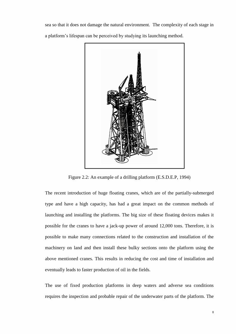

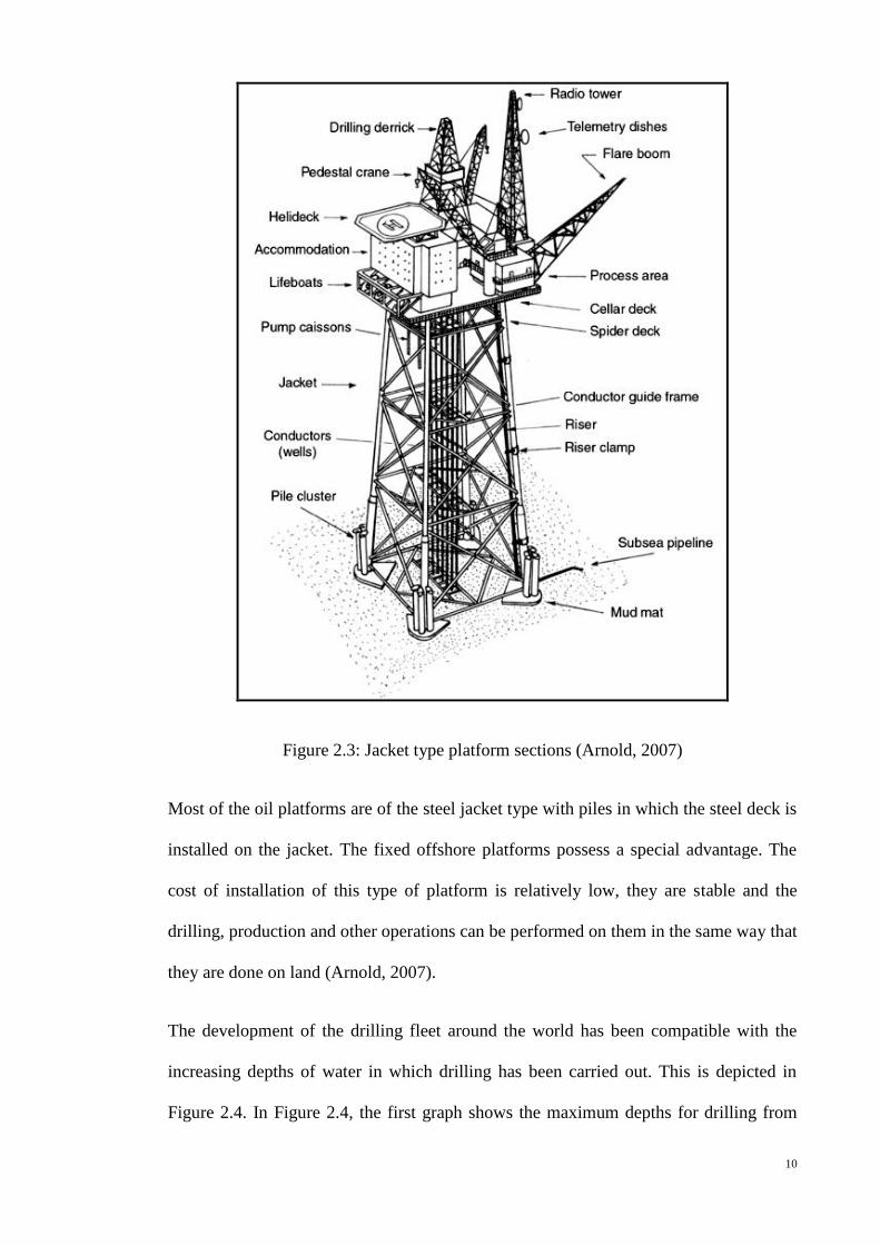


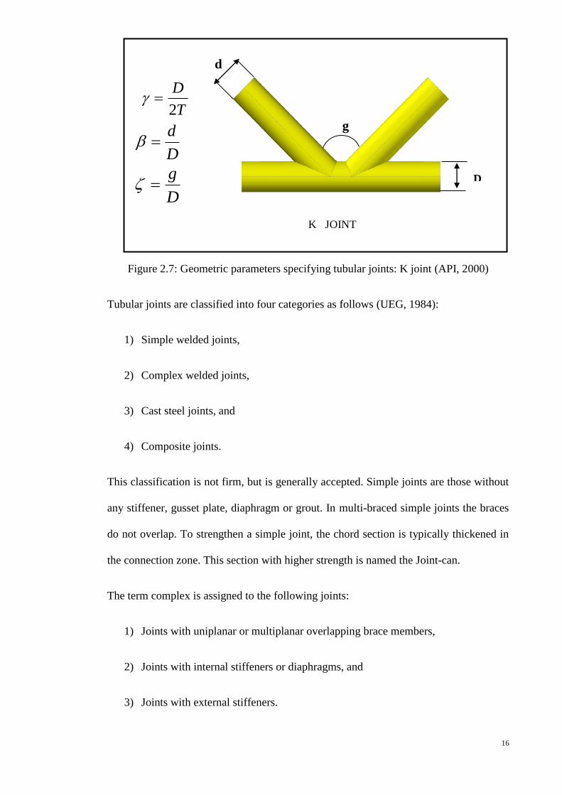
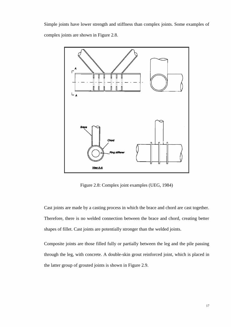


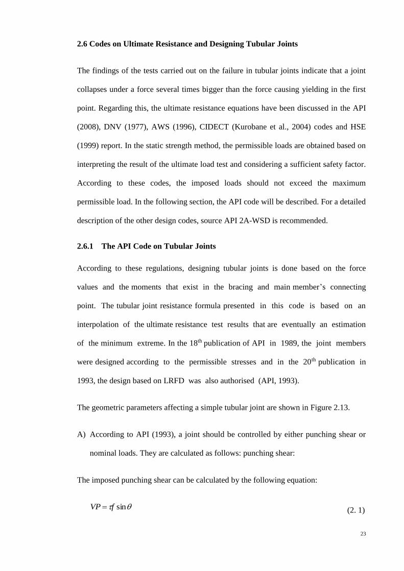


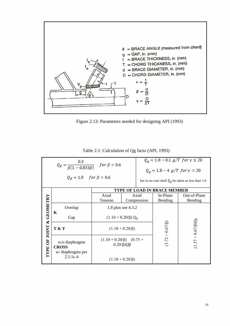


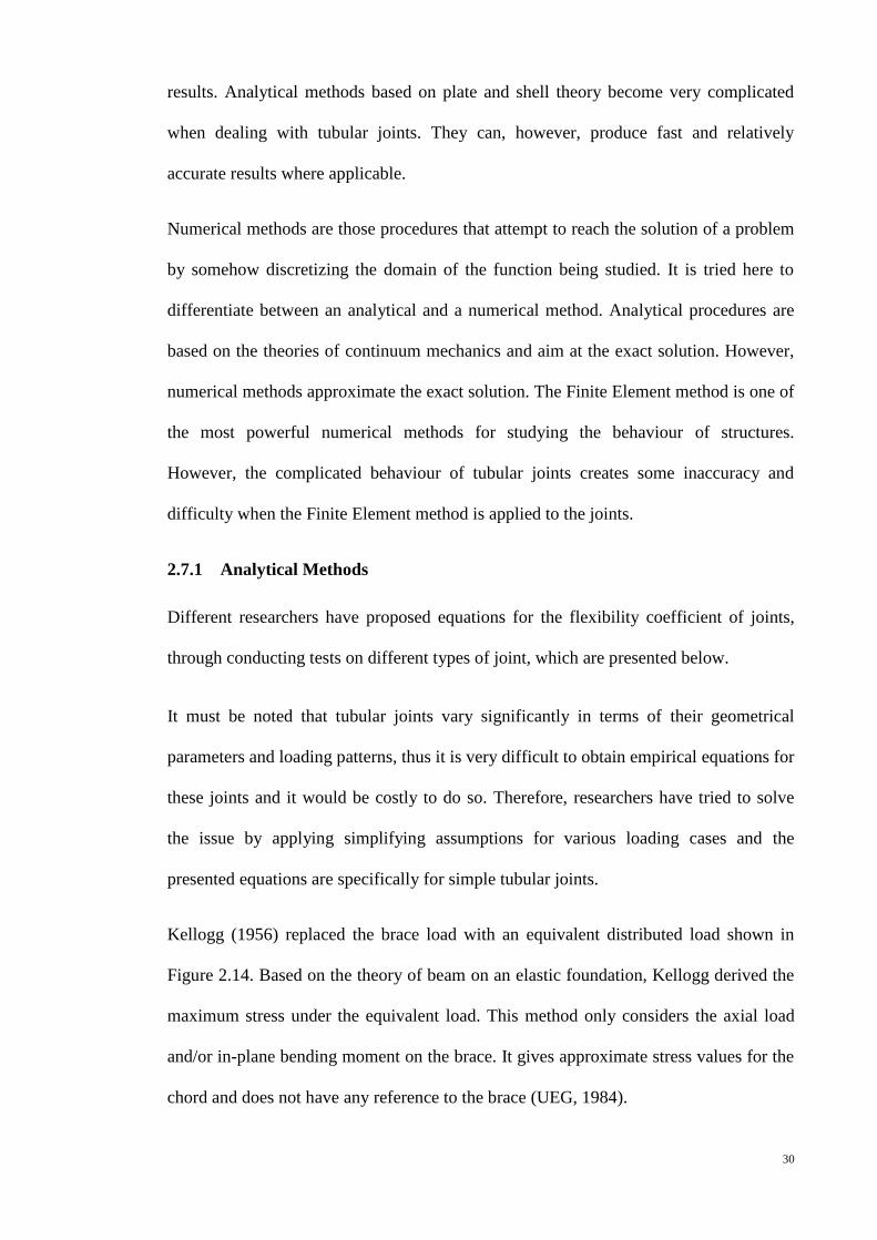
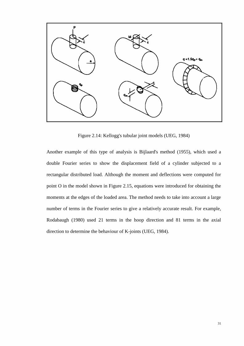


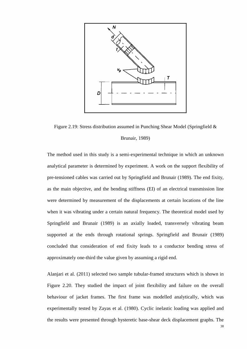
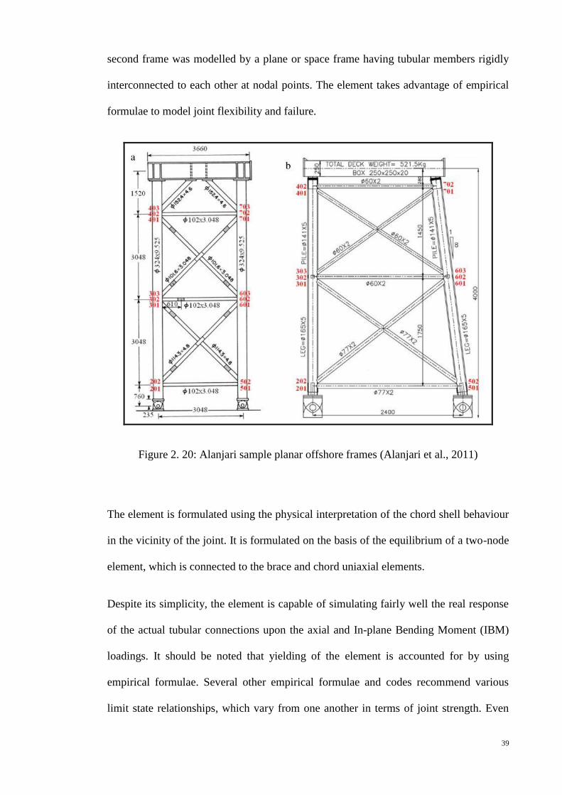
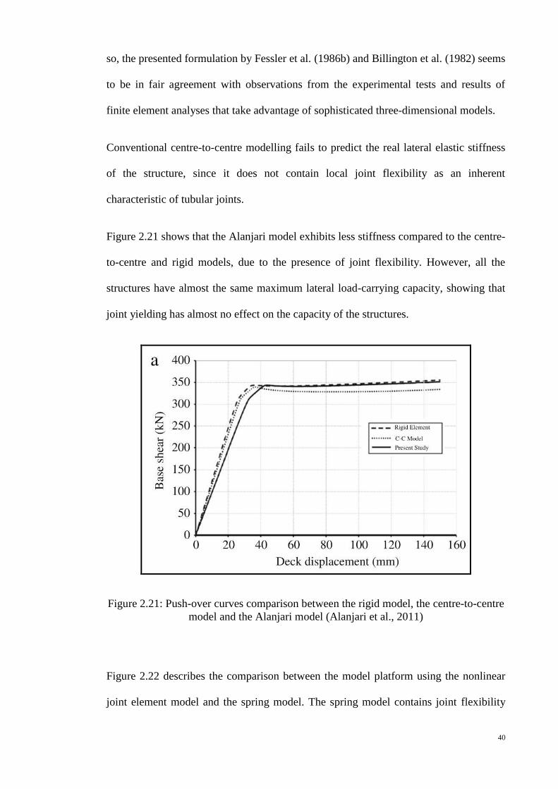


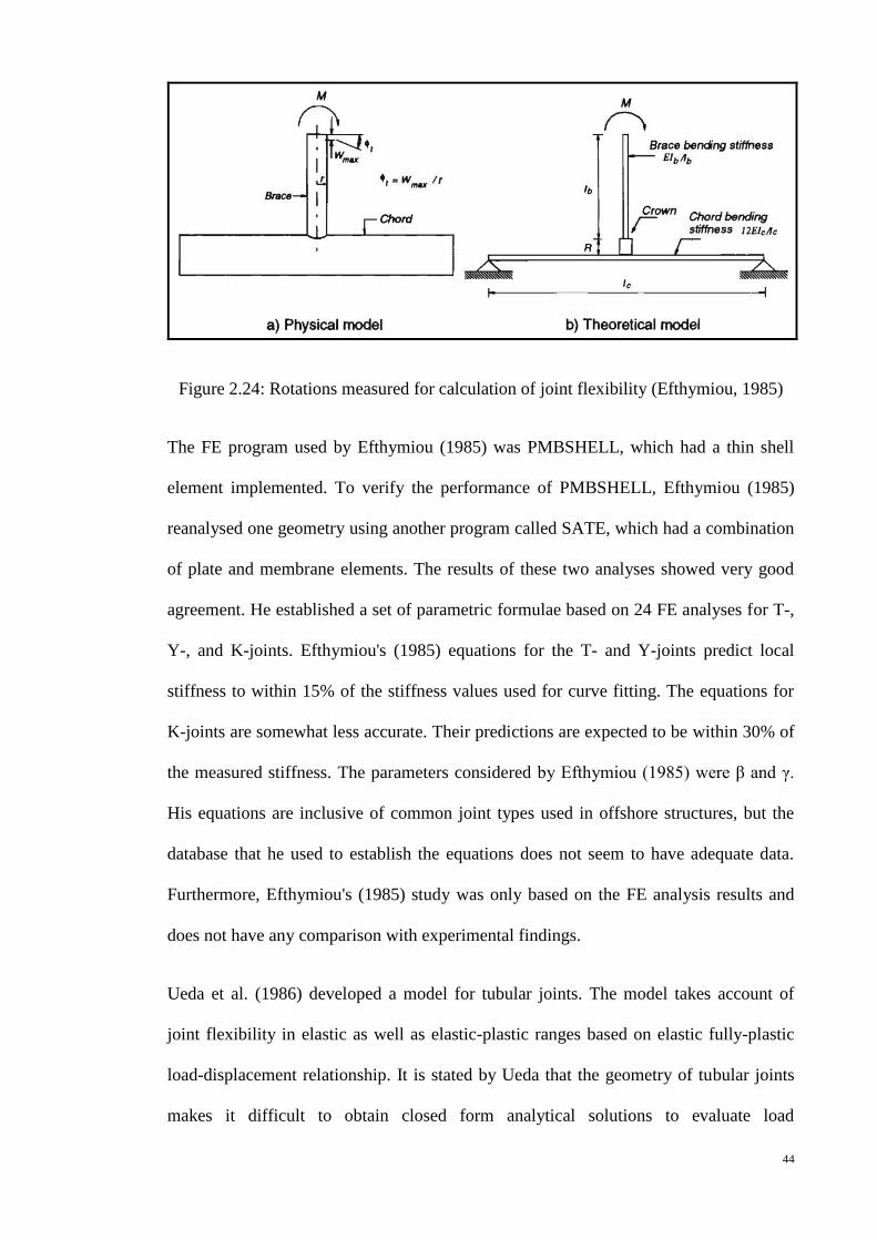


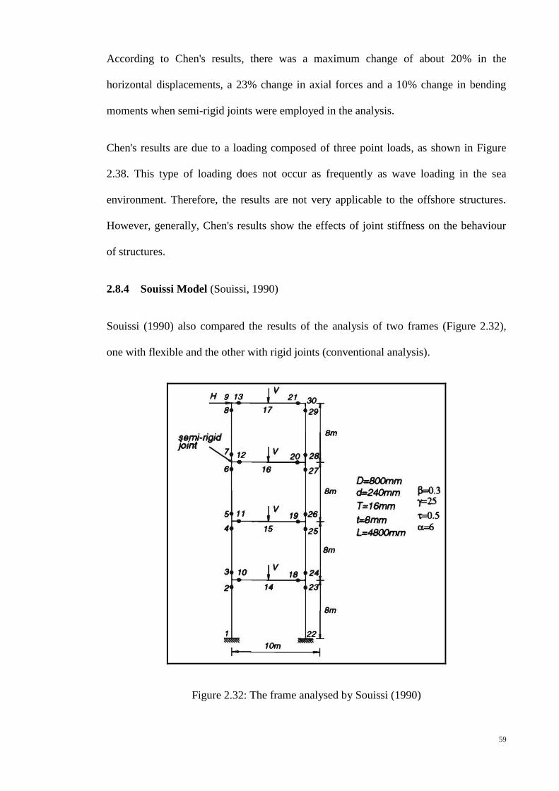


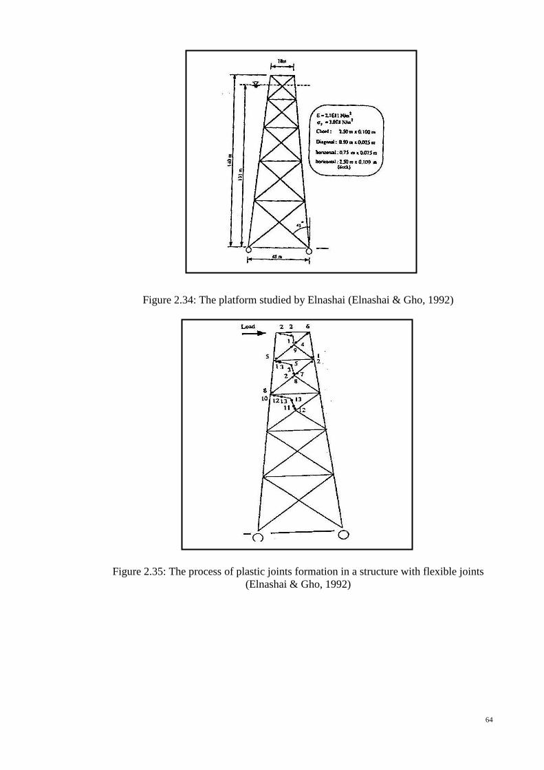


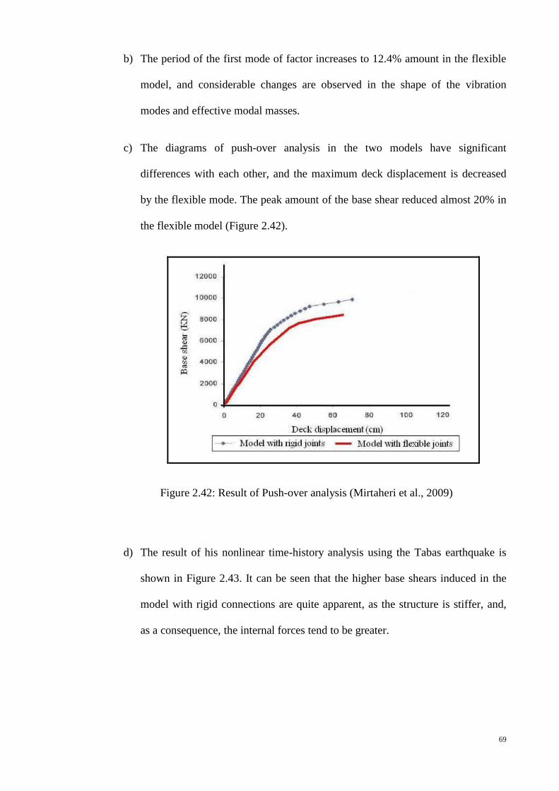


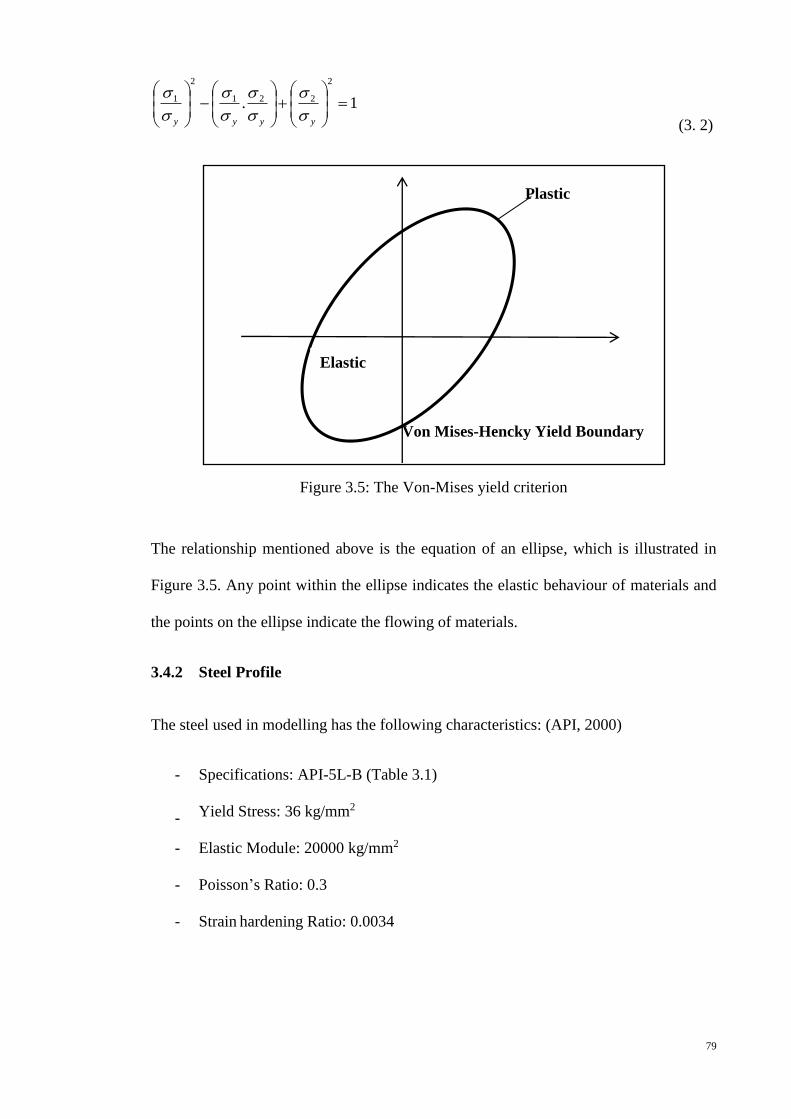


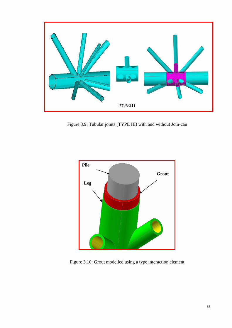


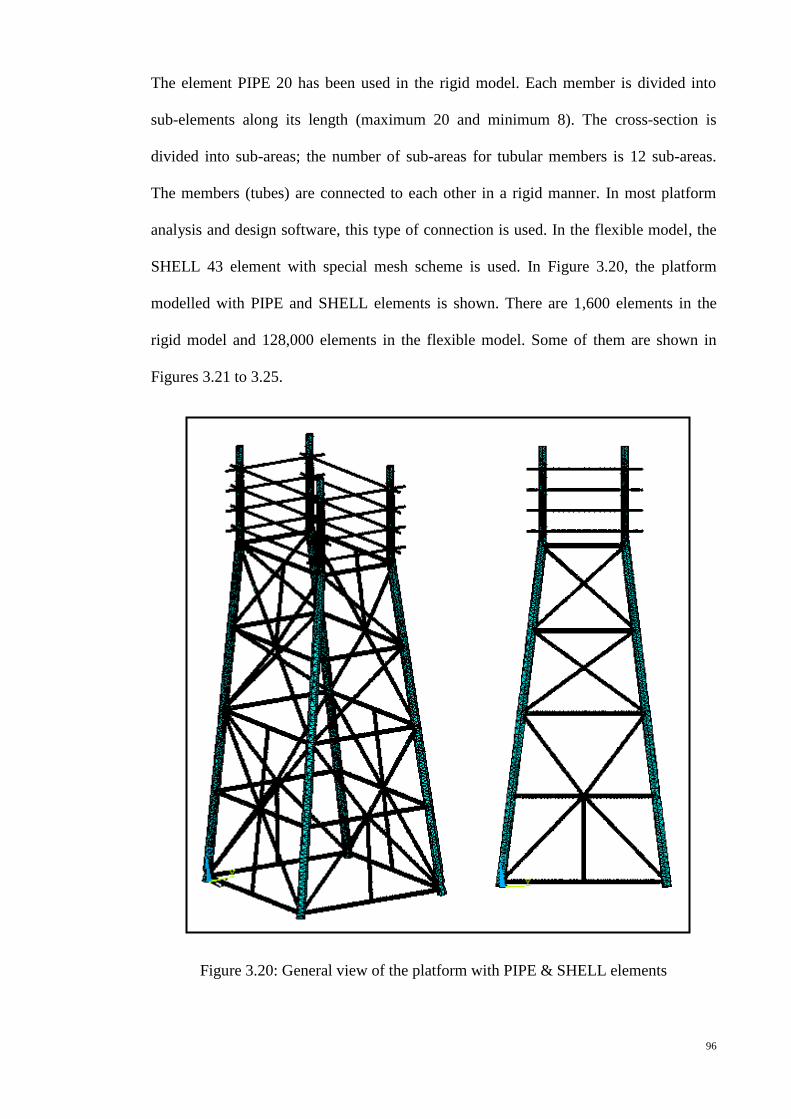


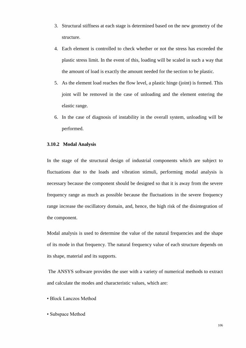


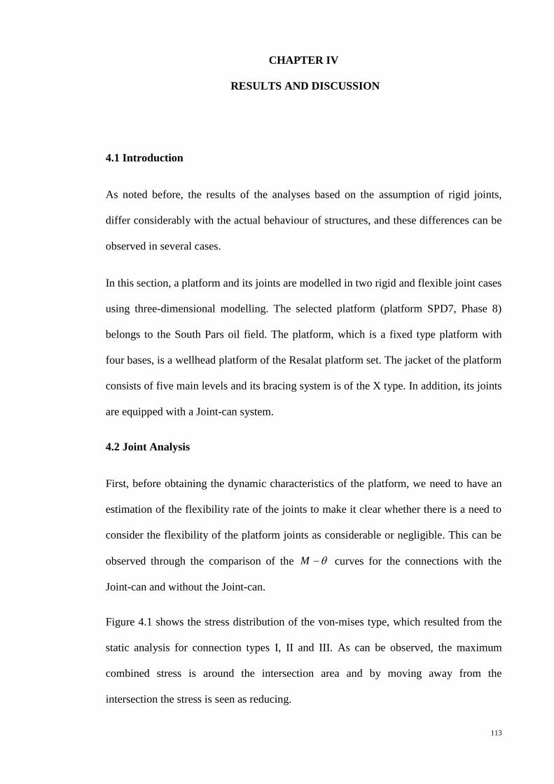


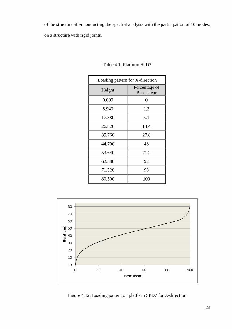


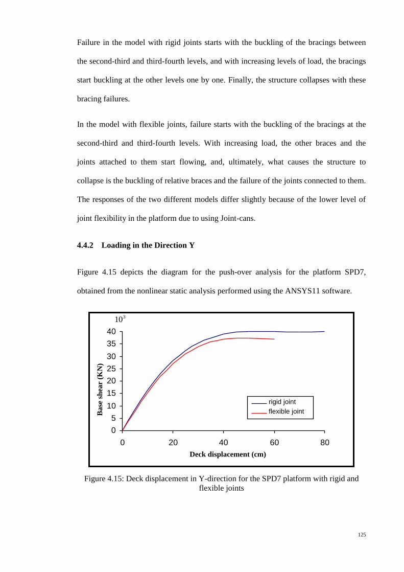


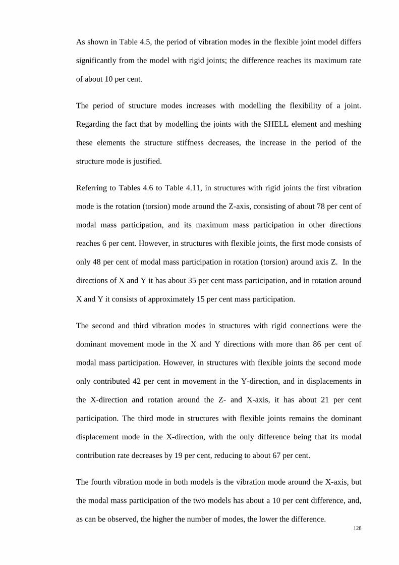


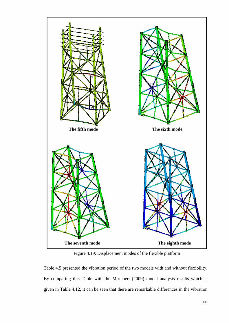

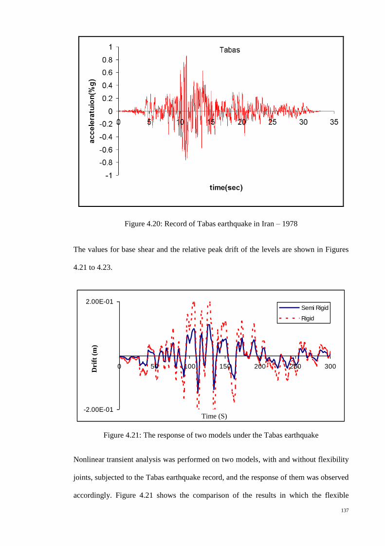


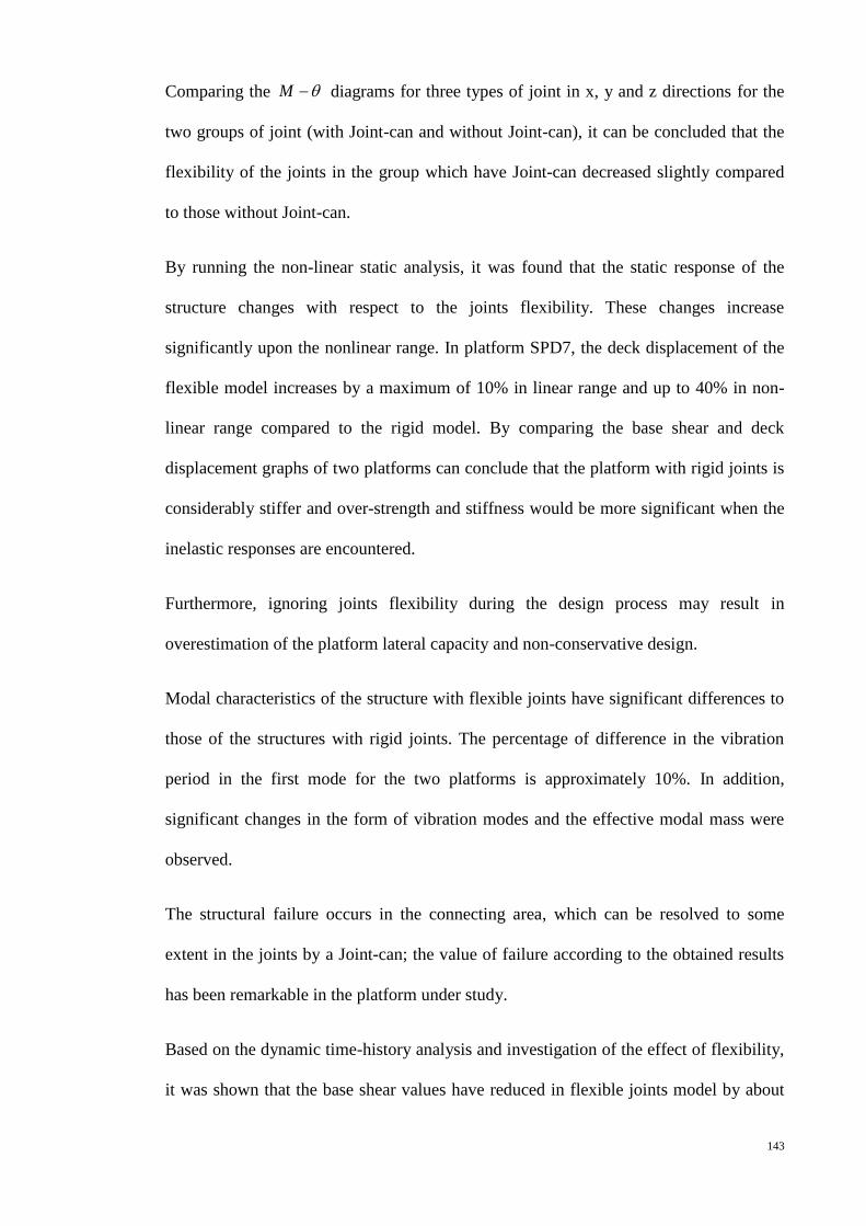


![SECTION DRAWINGS 07arahim/SECTION_DRAWINGS.pdfyang terdapat pada pandangan Sisi lukisan keratan objek. KERATAN A-A Title Microsoft PowerPoint - SECTION_DRAWINGS 07 [Compatibility Mode]](https://static.documents.pub/doc/80x56/608c0310279b9c46424bafa7/section-drawings-07-arahimsection-yang-terdapat-pada-pandangan-sisi-lukisan-keratan.jpg)

