Effect of Neighborhood on In-Network

Processing in Sensor Networks

Muhammad Jafar Sadeq and Matt Duckham

Department of Geomatics, The University of Melbourne, Victoria, 3010, Australiam.sadeq@pgrad.unimelb.edu.au, matt@duckham.org

Abstract. Wireless sensor networks are growing from a few hand-placeddevices to more large-scale networks in terms of coverage and node den-sity. For various concerns, such as scalability, larger network sizes requiresome management of the large volume of data that a sensor network de-livers. One way to manage this data is processing information in thenetwork. This paper investigates how a sensor network’s network ar-chitecture (specifically, the neighborhood structure) can influence theconclusions that a sensor network makes from its measurements. Theresults demonstrate that non-planar structures are infeasible for routingand some in-network processing applications. Structures with low aver-age edge lengths give better quantitative results, while those with highedge densities give better qualitative results.

1 Introduction

Wireless sensor networks (WSNs) are untethered networks of miniaturized sensor-enabled computers. WSNs are increasingly being used for geospatial applications,such as environmental monitoring. WSNs today typically use a periodic “sense-and-transmit” approach to transmit temporal snapshots of the entire network’sreadings to a centralized computing system [1][2]. The centralized computer sys-tem (such as a conventional GIS) is then tasked with analyzing the snapshotsto determine what significant events have occurred. As such, many of today’sWSN deployments can be regarded as sophisticated data loggers [3]. There areat least three important drawbacks to this approach:

– Energy resources : WSNs are highly resource constrained systems, in partic-ular with respect to sensor node energy resources. Wireless communicationis one of the most energy-intensive activities of a sensor node, so continuallyrelaying data to a central system can dramatically shorten the useful lifetimeof a WSN.

– Information overload : The fine-grained spatiotemporal detail becoming avail-able from larger sensor networks means that individual data items becomeless and less meaningful. Transmitting all data can lead to high levels ofredundancy and ultimately information overload.

– Sensor/actuator networks : The results of the analysis of sensor network dataare often required by the network itself in order modify the behavior of

the network (e.g., activate or deactivate sensors to adapt the granularity ofmonitoring depending on the activity of the environment, sometimes calledgeoresponsive sensor networks [4]). Removing information from the network,processing it centrally, then returning it to the network is an inefficient drainon network resources.

A growing proportion of current research in WSNs is dedicated to address-ing these problems using in-network processing, where sensor nodes themselvescollaborate in a decentralized manner to perform partial or complete processingof sensor data. This paper investigates how the structure of the network (linksbetween nodes) can influence the results of in-network processing of spatial in-formation and events.

Due to issues such as scalability, in-network processing often involves dis-tributed processing with nodes using information from their neighbors. The ques-tion then arises as to which nodes are considered neighbors of a particular node.Often, the simplest solution is taken, where a node has as its neighbors all nodesthat it can communicate with directly [5][6]. However, for routing, neighborhoodwill sometimes need to be limited to planar graphs (as discussed further in Sect.2). Therefore, multiple definitions of neighborhood may exist in the same WSN.This paper evaluates the use of different neighborhood structures for in-networkprocessing. Many of these structures are already used in routing research, thusgaining multiple uses out of a single infrastructure.

The importance of neighborhood structures to spatial applications can beseen when we realize that, for most environmental variables (such as temper-ature or light intensity), nodes take only point readings (with exceptions suchas cameras). There is often no knowledge of the readings between nodes, eitherin the WSN or in any central server. Neighborhood structures may be used toestimate these unsampled regions. Techniques such as Voronoi diagrams [7] canpartition the field into coverage areas in order to interpolate readings for theunsensed areas. Techniques such as kriging [8] estimate values at unsampledpoints. Given sufficient point estimates, point readings can be interpolated toa field. These techniques, however, may be computationally expensive when anode needs to do frequent interpolations in response to a dynamic environment.

From a qualitative spatial reasoning perspective, a fundamental interpolationprocess concerns the presence or absence of a boundary between neighboringnodes. Consider a binary region, for example a hot region (temperature> 25◦C)and its complement (temperature≤ 25◦C). If two nodes are connected topolog-ically, and one senses that it is in the hot region and the other senses that itis out of the hot region, it is certain that there exists a boundary of the hotregion boundary between them. If they both sense the hot region, it can be in-ferred that there is no boundary between them. An example is shown in Fig. 1.Based on a purely local, qualitative knowledge observations in their immediateneighborhood, Nodes A and D deduce that there must be a boundary between.Similarly, Nodes A and C can infer that there is no boundary between them.Thus, by answering a qualitative question (“Is there a boundary between myself

and my neighbor?”), the network topology can be used to build a picture of aregion.

Node in region:

Node out of region:

Key

Region boundaryestimated by network

H

A

G

C

D

F

E

B

Fig. 1. Use of network edges to build a region

In order to evaluate various neighborhood structures, this paper quantita-tively tests the ability of a WSN to approximate the boundary of a region whendifferent structures are applied to it. Boundary was chosen as an evaluation cri-terion because it is a fundamental construct for the detection of spatial eventsin region evolution — events occur at a region’s boundary or events create newboundaries. Boundary has salience for human spatial cognition and can be usedto represent various spatial properties of the region such as its shape or its area.This work also tests the neighborhood structures’ ability to qualitatively detecttopological events occurring to a region.

It has been found that non-planar structures are infeasible not only for rout-ing but can also cause inconsistencies in a WSN’s knowledge and state. Neigh-borhood structures with a lower average edge length gives better quantitativeresults. Those with high edge densities give better qualitative results. Higheredge densities usually increase the average edge length, so high edge densitiesresult in poorer quantitative performance.

2 Background

A lot of research effort has been given to developing neighborhood structuresfor WSNs because of their importance to routing. It is especially important togreedy routing, where a message is sent to a node geographically closer to thedestination than the current node. An example of a greedy routing algorithm isGreedy Perimeter Stateless Routing (GPSR) [9].

Greedy forwarding can fail if the message reaches a “void” where no nodeis closer to the destination than the current node. GPSR therefore includesprocedures to route around the edge of the void (Geographic Face Routing)[9][10]. Such forms of geographic routing (routing to a specific location) thereforerequire specific properties from the network graph of a WSN. One is that thenumber of voids must be minimized because face routing is more costly than

greedy forwarding. Another is that the graph must be planar (there must be nocrossing edges), otherwise face routing can fail. This in turn requires that thereare no uni-directional links [10].

Researchers use network graphs to test their algorithms and protocols. Occa-sionally, researchers compare various neighborhood structures for the purposes ofrouting. However, to our knowledge, there is no research on the effect of the var-ious neighborhood structures on the results of in-network processing. This maybe because there is little research so far into in-network processing of higher levelspatial information that rely on neighborhood structures.

This paper investigates how well different neighborhood structure approxi-mate the boundary of a region and how well they detect topological events. Anumber of boundary detection algorithms have been proposed in the literature.In the classifier approach, nodes estimate the location of a straight line repre-senting the local portion of the region boundary [5]. A node’s distance from thatline is used to determine whether it is a boundary node. In another approach, anode compares the average of the readings from its neighborhood to a thresholdin order to determine whether it is on the boundary [6].

By contrast, this paper adopts a qualitative approach where boundary nodesare identified purely from their relationship to immediate neighbors (i.e., whetheror not they neighbor a node on the opposite side of a boundary). In additionto simplifying the model and computation, adopting this qualitative approachcan help improve the network’s robustness to imperfection in sensor data andboundary indeterminary.

3 Neighborhood Structures

Modeling a network as a graph G = (S, E), with a set of vertices S ⊂ R2

representing sensor nodes as points in the plane and edges E ⊆ S×S representingthe potential for direct one-hop communication between nodes, the followingneighborhood structures are commonly used.

– Localized Delaunay triangulation: The Delaunay triangulation DT (S) is theunique triangulation of S such that no point in S is inside the circumcircleof any triangle in DT (S) [11]. A localized Delaunay triangulation (LDT) isa graph resulting from attempting to build a Delaunay triangulation (DT)using limited information (information local to a node). The LDT does nothave a complete convex hull since some edges that exceed the communica-tion range of the nodes are not included in the graph. Depending on thealgorithm, it may not even be a triangulation.

– Gabriel graph: E includes edges (x, y) and (y, x) between two points x ∈ Sand y ∈ S if the circle with xy as the diameter is free of other points in S[12]. GG(S) is a subgraph of DT (S).

– Relative neighborhood graph: E includes edges (x, y) and (y, x) if the lune(the intersection of the two circles with centers x and y and with xy asradius) is free of other points in S. RNG(S) is a subgraph of GG(S) [12].

– Localized greedy triangulation: The greedy triangulation GT (S) of a set ofpoints S is built by first creating a list of all edges between all nodes in thenetwork. The shortest edge is removed from the list and it is added to thetriangulation if it does not cross an edge that has already been inserted intothe triangulation. This continues until all the edges have been exhausted orthe number of edges in the triangulation is 3×N − 6, where N = |S|. Thusthe greedy triangulation (GT) attempts to minimize total edge length in agreedy manner [11]. The localized GT (LGT), built by nodes using localinformation, is not a complete triangulation, similar to LDT.

– Unit disk graph: UDG is a non-planar graph where there is an edge betweentwo points as long as the points are at most a unit distance apart. In aWSN, this is a graph where each node has edges to all nodes that it cancommunicate with.

The graphs can be compared in Fig. 2, which shows graphs built in a dis-tributed manner by a WSN simulation.

(c) RNG

(b) GG

(d) GT

(a) DT

(e) UDG

Fig. 2. Neighborhood structures built in a distributed manner

These five cover a variety of neighborhood structures. DT is well-known inspatial applications, so it is sensible to test a distributed version in a WSN. GGand RNG are built using completely local criteria and therefore lend themselvesto implementation in WSNs using distributed processing. GT’s usage of edgelength as a criterion may make it suitable for WSNs because many localizationalgorithms determine distance (using, for example, received signal strength) be-fore deriving coordinate information [13]. Finally, UDG is the most basic casewhere all possible edges between nodes exist.

4 Methodology

The neighborhood structures were compared against each other both quantita-tively and qualitatively. The quantitative properties of the neighborhood struc-tures were evaluated using a WSN’s approximation of the boundary of a region.Their qualitative properties were tested by determining their ability to detectcertain topological events. These tests were done by simulation.

4.1 Simulation Environment

It was infeasible to perform the tests using real sensor nodes due to the require-ment for a large number of nodes to make the spatial properties of the neighbor-hood structures meaningful. Therefore, the tests were done by simulation. Repast(http://repast.sourceforge.net/), a Java-based agent modeling tool, wasused. Each sensor node in the simulation was made an independent Java object.The field being simulated was also independent from the sensor nodes. The nodesinteract among each other and with the environment in a decentralized manner.

4.2 Decentralized Computation of Neighborhood Structures

In our simulations, the neighborhood structures were built by the nodes them-selves in a decentralized manner. Researchers have developed many decentralizedalgorithms to build network graphs that meet the routing requirements that havebeen mentioned in Sect. 2. The Cross-link Detection Protocol (CLDP) can gen-erate a planar subgraph of any arbitrary graph of the network [10]. A localizedDT built by a WSN can be ensured to be planar as long as a node uses informa-tion from nodes that are two communication hops away [14]. The Gabriel graph(GG) has also been used to develop network architectures [15], as it does notneed a special algorithm to be built by sensor nodes locally.

In our simulations, the GG and RNG were built by simply by each nodeapplying the GG and RNG rules (Sect. 3) to all nodes that it can communicatewith directly. Each node x ∈ S starts with a list of these nodes, which it canacquire in an initial handshaking phase. x tests each node in this list to checkwhether an edge between them is permitted in GG or RNG.

For the LDT, for every pair of nodes y and z in x’s communication range,if there were no nodes in the circumcircle of �xyz, edges (x, y) and (x, z) wereadded to E. Thus, for GG, RNG and LDT, the node does not compute thecomplete graph of all the points in its communication range.

If x uses nodes in its communication range to compute the LDT, a non-planar graph may result. This happens when x rejects a triangle �xyz due toa node w in �xyz’s circumcircle, but y or z accepts �xyz because w is out ofits communication range. This situation results in unidirectional links. If nodesthat are two communication hops away are included in the triangulation proce-dure, planarization is ensured [14]). For simplicity, however, in our simulationsx removed all unidirectional edges (each edge (x, y) for which y did not havean edge (y, x)). Additionally, triangles whose circumcircles include more than

three nodes were not included in the graph because they can result in crossinglinks. These procedures gave us a planar graph, but not a complete triangulation.Rather, the LDT is a graph based on the rules for Delaunay triangulation.

LGT requires the nodes to compute all possible edges between all its neigh-bors and create the complete graph to ensure no edges cross. Although fastalgorithms for GT exist in the literature, our objective in this work was not touse the most efficient algorithms but rather to test the neighborhood structures.Therefore, we used algorithms that were the simplest for us to implement, i.e.,we applied the basic rules of the neighborhood structures.

Finally, UDG was built by each node creating an edge to each other nodewithin .

4.3 Quantitative Test: L2 Error Norm

To quantitatively determine the accuracy of the region boundaries as approxi-mated by the WSN under various neighborhood structures, the shape, locationand size of the approximated region boundary were compared to the actualboundary. The L2 error norm provided a simple means to test all of these prop-erties. The L2 error norm is the area of the region enclosed between the bound-aries of two shapes. Given a region that a WSN is monitoring, it determines anapproximation P of the original region O. The L2 error norm was computed inthis paper by finding the area of the symmetric difference between O and P asa proportion of the total area of O, i.e.,

L2 error norm =area((O − P ) ∪ (P − O))

area(O). (1)

An L2 error norm of zero means that not only are the areas of the two shapesequal, but also that their boundaries are in complete agreement.

4.4 Qualitative Test: Detecting Topological Events

There exist six fundamental topological events for dynamic areal objects: ap-pearance and disappearance; merge and split; and self-merge and partial split[16].

1. Appearance/disappearance: A region or hole appears or disappears.2. Merge/split: Two disconnected region components meet and become con-

nected, or a region component splits into two disconnected components.3. Self-merge/partial-split: A hole is formed in a region by engulfing part of it’s

exterior (self-merge) or a hole is destroyed in a region by its merging withthe region’s exterior (partial-split).

Examples of the six fundamental topological events are shown in Fig. 3.In a concurrent work, we have developed an algorithm to detect these events

and distinguish them from each other and from non-topological events (expan-sion and contraction). For several reasons, including space limitation, only merge

a.Appearance

Disappearance

b.Merge

Split

c.Self-Merge

Partial-Split

Fig. 3. Six fundamental topological events for dynamic areal objects

and split are investigated in this paper. Partial-split is not investigated becausethe algorithm to detect it is not independent, relying on previous events be-ing identified correctly. Self-merge is left out because it is similar to split inits requirements from a neighborhood structure. Misidentified appearances anddisappearances usually result in incorrect detections of other events (split andmerge), therefore it was felt that merge and split were suitably representative oftopological events to be used to analyze the neighborhood structures’ effective-ness.

The complete algorithm to detect and distinguish spatial events is beyondthe scope of these paper. In fact, the algorithm for detecting a merge is notneeded to understand why a merge can be incorrectly detected, so that is leftout too. Only a condensed version for the detection of split is presented.

Split Detection The algorithm for detection of a split is complicated due to thedifficulty in distinguishing it from contraction. In both Fig. 4(a) and Fig. 4(b),Node A has detected a change in the environment. Consequently, the regionbeing monitored no longer includes A. To differentiate split and contraction,Node A maintains its neighbors in a list sorted by direction (called the cyclicordering of the neighbors). With this sorted list, it determines how many blocksof region/hole surround it.

A CB A CBSplit

A CB A CBContract

E

D

E

D

E

D

E

D

(a)

(b)

Fig. 4. Split/contract

If there are two such blocks, the region has contracted — in Fig. 4(a), A issurrounded by an in-region block consisting of B, D and C and an out-of-regionblock consisting of only E. If there are four or more blocks (Fig. 4(b): B, D, Cand E are all in separate blocks around A), the region has split.

To demonstrate why four blocks are necessary, consider D. If D were notin A’s neighborhood, A would not be able to determine whether a split hasoccurred. This is because, from A’s point of view, there is a consecutive blockof region around it consisting of B and C. It therefore assumes that a contrac-tion has occurred. Additionally, the absence of D means that A cannot locallydetermine whether the region is connected beyond its immediate neighborhood.

Further cases (such as if D is actually in a hole in the region) are easilyresolved, but those issues are beyond the scope of the paper. In our simulationsto evaluate neighborhood structures, we controlled the region evolution so thatonly merge and split occurred. Therefore, in this paper, it is not necessary todiscuss the complete algorithm. Instead, it is sufficient to realize that, to detecta split, a node must have at least four neighbors.

5 Boundary Approximation and Analysis

One hundred random deployments of 500 nodes were generated for the simula-tions to determine which of the neighborhood structures gave rise to the bestboundary approximation from the WSN. For each of the hundred deployments,each of the neighborhood structures was applied.

5.1 Experiment 1: Polygonal Region

In a binary field, the WSN was used to monitor a simple polygonal region (Fig. 5).In order to determine the WSN’s boundary approximation, a message is passedalong the boundary of the region (usually the nodes just inside the boundary).

The message collects a list of boundary coordinates as it moves from node tonode along the region boundary. The message is passed anticlockwise along theregion boundary — this was an arbitrary choice. The ordered list of coordinatesthat results from this message is the WSN’s polygonal approximation of theactual region boundary.

Fig. 5. Example of LGT-networked WSN monitoring a polygonal region

Figure 6 can be used to demonstrate how the WSN builds its polygonalapproximation of the region boundary. The nodes maintain their neighbor ta-bles sorted by cyclic ordering around the node. For example, B’s anticlockwiseneighbor list may be (I, A, C, H). Let B be the initiator of the boundary approx-imation task. From the ordered list of its neighbors, H is the first neighbor of Bthat is outside the region (since it directly follows a neighbor that is inside theregion). B starts the boundary polygon with the midpoint of BH . It then addsmidpoint of BI to the polygon. Since the next neighbor in the list, A, is insidethe region, the list of coordinates is passed to A. A adds the midpoints of AJ ,AK, AE and AD to the list, then passes it on to C. When the list of coordinatesreturns to B, it receives the complete estimate of the boundary polygon.

Results Figure 7 (one of 100 simulations) gives a qualitative view of the WSN’sapproximation of the monitored region’s boundary using the different neighbor-hood structures. Table 1 gives the average L2 error norm for the 100 simulationsfor each neighborhood structure. The results show that RNG is the best at es-timating a region boundary, while LGT is the worst.

T-tests were performed to determine whether the differences between thevarious neighborhood structures were statistically significant at the 5% level.The tests revealed that they were significantly different, even LDT and LGT,which were very close in results with a 0.001 difference in L2 error norm.

Node in region:

Node out of region:

KeyJ

A

C

D

F

E

B

G

H

I

K

Actual region boundary:

Estimated region boundary:

Vertex on estimatedboundary polygon:

Fig. 6. A simple example of a WSN’s polygonal estimate of a region boundary

Table 1. Average L2 error norms for the polygonal region

Neighborhood Structure Average L2 error norm

LGT 0.106LDT 0.105GG 0.0971

RNG 0.0919

Absence of UDG from Results Observe that the results do not include theUDG. This is due to the nature of the message transmission scheme in Sect.5.1 (tracing around a boundary), which is a form of face routing since messagesare sent along edges according to their cyclic order. This has the pitfalls ofgeographic face routing, and so non-planar graphs cause the message to loopforever. An example is shown in Fig. 8. A message arrives at D (1), is passedto B (2), then to A (3), C (4) and back to B (5), at which point it continuesalong path 3-4-5. Observe that removing either the edge DB or CA (making thegraph planar) can solve the problem. The UDG is intrinsically non-planar, andso is unsuitable to the distributed boundary approximation algorithm above.

Discussion It was expected that the neighborhood structures with higher edgedensity (such as LDT and LGT) would perform better because the higher numberof edges would allow the network to trace around the boundary more accurately.However, the results showed that RNG performed the best.

A reason for this unexpected result is that RNG is the sparsest of the fourneighborhood structures. It therefore has fewer edges that intersect the region’sboundary, and consequently the WSN’s estimate of the region boundary hasfewer vertices. This results in fewer and longer edges in the approximation poly-gon. This seemed a good explanation for why RNG was best at monitoring thesimulated region of few vertices and long linear edges 5.

DTGG

GTRNG

Fig. 7. Approximations of the polygonal region boundary using different neighborhoodstructures

5.2 Experiment 2: Circular Region

The results of Experiment 1 suggested that shapes with linear edges were bestmonitored by a WSN with RNG. Therefore, experiment was repeated with aregion without straight lines — the circular region in Fig. 9.

Results Figure 10 is a sample of the shape of the boundary approximationsdue the the four neighborhood structures.

The L2 error norm, averaged over 100 simulation runs, showed that RNG hasthe best results again (Table 2). The results were statistically significant at the5% level, and they were also correlated — whenever one neighborhood structurework well, the others work well too (Pearson correlations of between 0.845 and0.942). The exception was RNG, which was comparatively uncorrelated (Pearsoncorrelations of between 0.578 and 0.674).

Discussion Contrary to our expectations, RNG performed better in both cir-cular and polygonal regions. An explanation for this is that RNG is sparser than

A

B

D C

1

2

34

5

RegionBoundary

E

Fig. 8. Non-planar neighborhood causes an infinite loop

Fig. 9. Example of GT-networked WSN monitoring a circular region

the other structures in terms of edge density. Its edges are therefore shorter thanthose of GG and DT, of which it is a subgraph. Whenever one of the RNG edgesintersect the region boundary, the likelihood is that any point on the edge iscloser to the actual boundary location than any point on the longer edges ofLDT. Due to this low average edge length of RNG, its boundary points were onaverage the most accurate.

The results for the circular region were better than the polygonal region dueto the sharp corners of the polygonal region. The WSN is not always able toestimate correctly these sharp turns of the polygon boundary.

6 Detection of Topological Events

It has been seen that the low edge density, and consequently the low averageedge length, of RNG makes it suited to locating the boundary. The following

DTGG

GTRNG

Fig. 10. Approximations of the circular region boundary using different neighborhoodstructures

experiments determine how the neighborhood structures perform in detectingtopological events.

6.1 Experiment 3: Merge

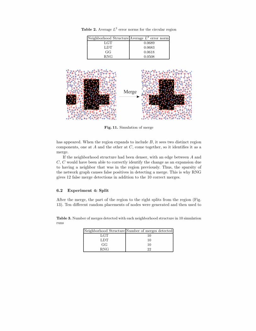
In these experiments, a small square region component moves until it merges withthe polygonal region component (Fig. 11). For each neighborhood structure, weran the simulation with ten different random deployments of nodes. For eachsimulation run, we counted how many merges were detected.

Results WSNs under LDT, GG and LGT detected exactly one merge corre-sponding to the merge event in Fig. 11. RNG, however, detected 12 additionalmerges (Table 3).

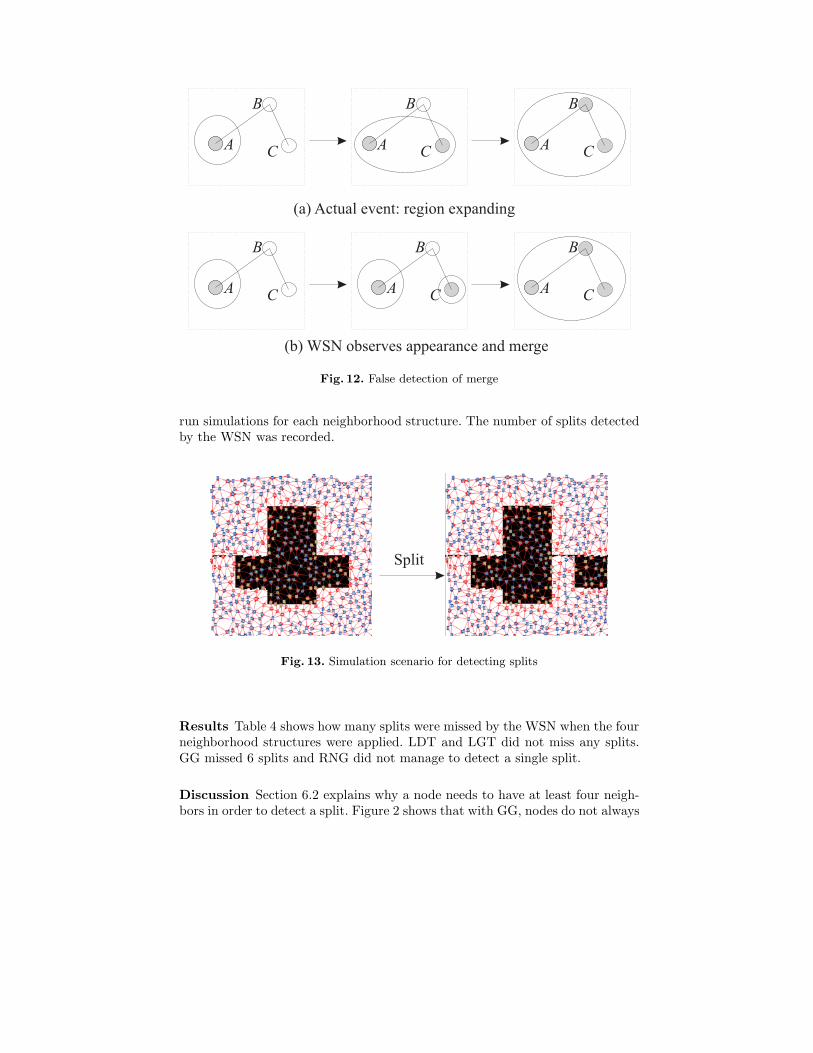
Discussion Figure 12 demonstrates how a WSN may incorrectly identify amerge. Figure 12(a) shows a region expanding. Figure 12(b) shows the WSN’sbelief of what is occurring. Since A and C are disconnected, their detections ofthe region are treated as separate. So C believes that a new region component

Table 2. Average L2 error norms for the circular region

Neighborhood Structure Average L2 error norm

LGT 0.0689LDT 0.0683GG 0.0618

RNG 0.0508

Merge

Fig. 11. Simulation of merge

has appeared. When the region expands to include B, it sees two distinct regioncomponents, one at A and the other at C, come together, so it identifies it as amerge.

If the neighborhood structure had been denser, with an edge between A andC, C would have been able to correctly identify the change as an expansion dueto having a neighbor that was in the region previously. Thus, the sparsity ofthe network graph causes false positives in detecting a merge. This is why RNGgives 12 false merge detections in addition to the 10 correct merges.

6.2 Experiment 4: Split

After the merge, the part of the region to the right splits from the region (Fig.13). Ten different random placements of nodes were generated and then used to

Table 3. Number of merges detected with each neighborhood structure in 10 simulationruns

Neighborhood Structure Number of merges detected

LGT 10LDT 10GG 10

RNG 22

(a) Actual event: region expanding

(b) WSN observes appearance and merge

AC

B

A

B

A

B

A

B

A

B

A

B

C C

C C C

Fig. 12. False detection of merge

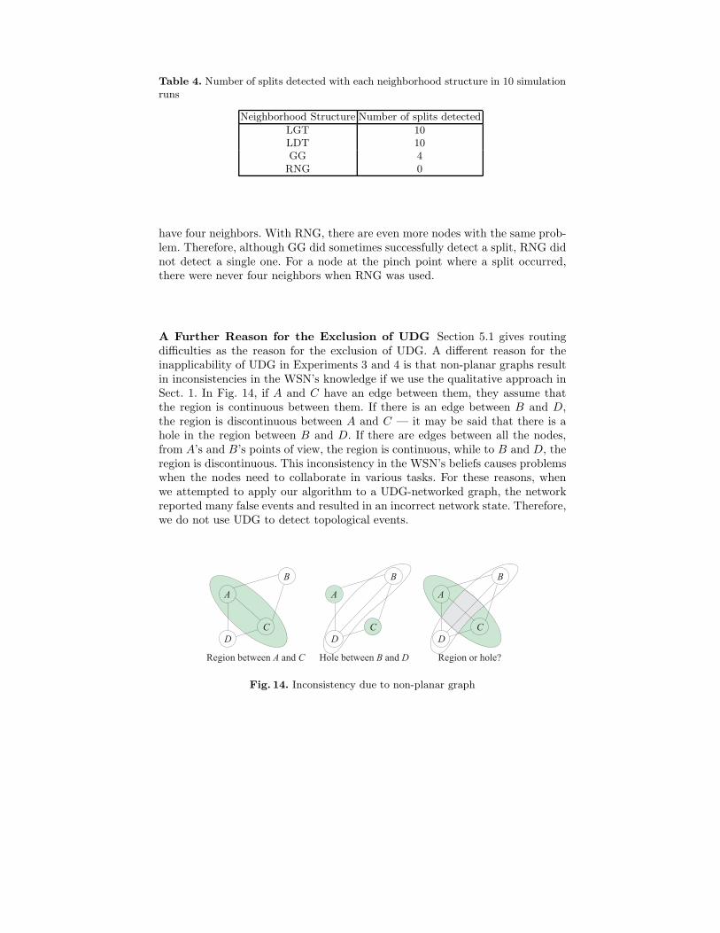
run simulations for each neighborhood structure. The number of splits detectedby the WSN was recorded.

Split

Fig. 13. Simulation scenario for detecting splits

Results Table 4 shows how many splits were missed by the WSN when the fourneighborhood structures were applied. LDT and LGT did not miss any splits.GG missed 6 splits and RNG did not manage to detect a single split.

Discussion Section 6.2 explains why a node needs to have at least four neigh-bors in order to detect a split. Figure 2 shows that with GG, nodes do not always

Table 4. Number of splits detected with each neighborhood structure in 10 simulationruns

Neighborhood Structure Number of splits detected

LGT 10LDT 10GG 4

RNG 0

have four neighbors. With RNG, there are even more nodes with the same prob-lem. Therefore, although GG did sometimes successfully detect a split, RNG didnot detect a single one. For a node at the pinch point where a split occurred,there were never four neighbors when RNG was used.

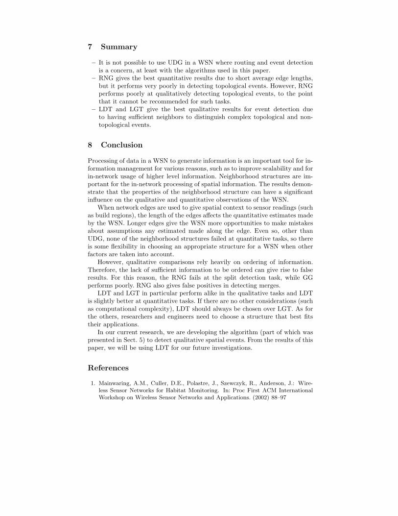
A Further Reason for the Exclusion of UDG Section 5.1 gives routingdifficulties as the reason for the exclusion of UDG. A different reason for theinapplicability of UDG in Experiments 3 and 4 is that non-planar graphs resultin inconsistencies in the WSN’s knowledge if we use the qualitative approach inSect. 1. In Fig. 14, if A and C have an edge between them, they assume thatthe region is continuous between them. If there is an edge between B and D,the region is discontinuous between A and C — it may be said that there is ahole in the region between B and D. If there are edges between all the nodes,from A’s and B’s points of view, the region is continuous, while to B and D, theregion is discontinuous. This inconsistency in the WSN’s beliefs causes problemswhen the nodes need to collaborate in various tasks. For these reasons, whenwe attempted to apply our algorithm to a UDG-networked graph, the networkreported many false events and resulted in an incorrect network state. Therefore,we do not use UDG to detect topological events.

A

C

D

B

A

C

D

B

A

C

D

B

Region between andA C Hole between andB D Region or hole?

Fig. 14. Inconsistency due to non-planar graph

7 Summary

– It is not possible to use UDG in a WSN where routing and event detectionis a concern, at least with the algorithms used in this paper.

– RNG gives the best quantitative results due to short average edge lengths,but it performs very poorly in detecting topological events. However, RNGperforms poorly at qualitatively detecting topological events, to the pointthat it cannot be recommended for such tasks.

– LDT and LGT give the best qualitative results for event detection dueto having sufficient neighbors to distinguish complex topological and non-topological events.

8 Conclusion

Processing of data in a WSN to generate information is an important tool for in-formation management for various reasons, such as to improve scalability and forin-network usage of higher level information. Neighborhood structures are im-portant for the in-network processing of spatial information. The results demon-strate that the properties of the neighborhood structure can have a significantinfluence on the qualitative and quantitative observations of the WSN.

When network edges are used to give spatial context to sensor readings (suchas build regions), the length of the edges affects the quantitative estimates madeby the WSN. Longer edges give the WSN more opportunities to make mistakesabout assumptions any estimated made along the edge. Even so, other thanUDG, none of the neighborhood structures failed at quantitative tasks, so thereis some flexibility in choosing an appropriate structure for a WSN when otherfactors are taken into account.

However, qualitative comparisons rely heavily on ordering of information.Therefore, the lack of sufficient information to be ordered can give rise to falseresults. For this reason, the RNG fails at the split detection task, while GGperforms poorly. RNG also gives false positives in detecting merges.

LDT and LGT in particular perform alike in the qualitative tasks and LDTis slightly better at quantitative tasks. If there are no other considerations (suchas computational complexity), LDT should always be chosen over LGT. As forthe others, researchers and engineers need to choose a structure that best fitstheir applications.

In our current research, we are developing the algorithm (part of which waspresented in Sect. 5) to detect qualitative spatial events. From the results of thispaper, we will be using LDT for our future investigations.

References

1. Mainwaring, A.M., Culler, D.E., Polastre, J., Szewczyk, R., Anderson, J.: Wire-less Sensor Networks for Habitat Monitoring. In: Proc First ACM InternationalWorkshop on Wireless Sensor Networks and Applications. (2002) 88–97

2. Hamilton, M.P., Graham, E., Rundel, P.W., Allen, M.F., Kaiser, W., Hansen, M.H.,Estrin, D.L.: New Approaches in Embedded Networked Sensing for TerrestrialEcological Observatories. Environmental Engineering Science 24(2) (2007)

3. Hart, J.K., Martinez, K.: Environmental Sensor Networks: A Revolution in theEarth System Science? Earth-Science Reviews 78 (2006) 177–191

4. Duckham, M., Nittel, S., Worboys, M.F.: Monitoring Dynamic Spatial Fields UsingResponsive Geosensor Networks. In: GIS’05: Proc 13th Annual ACM InternationalWorkshop on Geographic Information Systems, New York, NY, USA, ACM Press(2005) 51–60

5. Chintalapudi, K., Govindan, R.: Localized Edge Detection in Sensor Fields. AdHoc Networks 1(2-3) (2003) 273–291

6. Jin, G., Nittel, S.: NED: An Efficient Noise-Tolerant Event and Event BoundaryDetection Algorithm in Wireless Sensor Networks. In: MDM ’06: Proceedings ofthe 7th International Conference on Mobile Data Management (MDM’06), Wash-ington, DC, USA, IEEE Computer Society (2006) 153

7. de Berg, M., van Kreveld, M., Overmars, M., Schwarzkopf, O.: ComputationalGeometry: Algorithms and Applications. Springer-Verlag (1997)

8. Barnett, V.: Environmental Statistics: Methods and Applications. Wiley (2004)9. Karp, B., Kung, H.T.: GPSR: Greedy Perimeter Stateless Routing for Wireless

Networks. In: MobiCom ’00: Proceedings of the 6th Annual International Con-ference on Mobile Computing and Networking, New York, NY, USA, ACM Press(2000) 243–254

10. Kim, Y.J., Govindan, R., Karp, B., Shenker, S.: On the Pitfalls of Geographic FaceRouting. In: Proceedings of the Third ACM/SIGMOBILE International Workshopon Foundations of Mobile Computing, New York, NY, USA, ACM Press (Septem-ber 2005) 34–43

11. Preparata, F.P., Shamos, M.I.: Computational Geometry: An Introduction.Springer-Verlag New York, Inc., New York, NY, USA (1985)

12. Zhao, F., Guibas, L.: Wireless Sensor Networks: An Information Processing Ap-proach. Elsevier/Morgan-Kaufmann, Amsterdam (2004)

13. Vaidyanathan Ramadurai, M.L.S.: Localization in Wireless Sensor Networks: AProbabilistic Approach. In Zhuang, W., Yeh, C.H., Droegehorn, O., Toh, C.T.,Arabnia, H.R., eds.: Proceedings of the International Conference on Wireless Net-works, Las Vegas, Nevada, USA, CSREA Press (June 2003) 275–281

14. Li, X.Y., Calinescu, G., Wan, P.J., Wang, Y.: Localized Delaunay Triangulationwith Application in Ad Hoc Wireless Networks. IEEE Transactions on Paralleland Distributed Systems 14(10) (2003) 1035–1047

15. Funke, S., Milosavljevic, N.: Infrastructure-Establishment from Scratch in WirelessSensor Networks. In: Distributed computing in sensor systems : First IEEE In-ternational Conference, DCOSS 2005. Volume 3560 of Lecture Notes in ComputerScience., Marina Del Rey, USA (2005) 354–367

16. Jiang, J., Worboys, M.F.: Event-Based Topology for Dynamic Planar Areal Object.International Journal of Geographical Information Science (2008) Under review.