University of Mississippi University of Mississippi

eGrove eGrove

Electronic Theses and Dissertations Graduate School

1-1-2017

Effect of Vibration of Unconsolidated Sand on the Performance of Effect of Vibration of Unconsolidated Sand on the Performance of

Interferometric Vibration Sensors Interferometric Vibration Sensors

Cody Berrey University of Mississippi

Follow this and additional works at: https://egrove.olemiss.edu/etd

Part of the Mechanical Engineering Commons

Recommended Citation Recommended Citation Berrey, Cody, "Effect of Vibration of Unconsolidated Sand on the Performance of Interferometric Vibration Sensors" (2017). Electronic Theses and Dissertations. 1332. https://egrove.olemiss.edu/etd/1332

This Thesis is brought to you for free and open access by the Graduate School at eGrove. It has been accepted for inclusion in Electronic Theses and Dissertations by an authorized administrator of eGrove. For more information, please contact egrove@olemiss.edu.

EFFECT OF VIBRATION OF UNCONSOLIDATED SAND ON THE PERFORMANCE OF

INTERFEROMETRIC SENSORS

A Thesis

presented in partial fulfillment of requirements

for the degree of Master of Science

in the Department of Mechanical Engineering

The University of Mississippi

by

CODY S. BERREY

May 2017

Copyright Cody S. Berrey 2017

ALL RIGHTS RESERVED

ii

ABSTRACT

Interferometric vibration sensors are widely used for ground vibration measurements

where traditional contact sensors are not desired. Laser Doppler vibrometers (LDV) and digital

speckle pattern interferometers are studied in this thesis. The working principle of laser Doppler

vibrometry and digital shearography is described. The effect of vibration of the unconsolidated

sand on the performance of both sensors is experimentally investigated.

The vibration of unconsolidated sand can cause an increase of noise in the laser Doppler

vibrometer output and cause speckle decorrelation in digital speckle pattern interferometry

(referred to as digital shearography). An experimental investigation of the effect of varying the

grain size and the vibration amplitude of sand is conducted. The experiments are two-fold: the

first experiment focuses on digital shearography ground vibration measurements on ten different

sands with varying grain size ranges to study the effect of speckle decorrelation on the

performance of digital shearography; and, the second experiment utilizes the LDV to measure

the same ten sands at incrementally higher vibration amplitudes to see the effect of sand particle

motion on the performance and noise of the LDV.

It was found that for digital shearography, the vibration amplitude necessary to cause

speckle decorrelation decreased from 4.18μm to 2μm for the increase in grain size from 0.15mm

to 1mm. For the LDV, it was found that the average increase in noise is between 34.2dB and

45.6dB for an increase in vibration amplitude of 2μm to 22μm.

iii

DEDICATION

I dedicate this work to the family and friends who have supported me during my six years

at Ole Miss. A special thanks to my loving parents. Without their love and support, I would not

be the person I am today. Also, to my grandfather, Frank Mitchell (1932-2012), I will always

cherish the stories that he shared with me growing up.

This work is also dedicated to Dr. Jim Chambers (1968-2016). He was an advisor,

mentor, and most importantly, a friend. Without him I would not be in graduate school today.

iv

ACKNOWLEDGMENTS

I would like to acknowledge the contributions of the faculty of the NCPA and the

Department of Mechanical Engineering for helping me get to this point in both my

undergraduate and graduate degree programs. A special thanks to Dr. Craig Hickey and Dr. Sara

Brown for their constant guidance in my four years at the NCPA and also to Dr. Raj, who has

been my academic advisor since Freshman year, thank you for guiding me through the last six

years of academic work.

A special thank you to Dr. Vyacheslav Aranchuk who has been the best research advisor,

mentor, and friend I could have asked for. I have had the privilege to work under you for almost

four years, and I most certainly would not be in graduate school today or have the excellent job

opportunities I currently have if not for you.

I would like to also acknowledge the Office of Naval Research for supporting this work

under grant #N000141210202. The views and conclusions contained in this document are those

of the author and should not be interpreted as representing the official policies, either expressed

or implied, of the Office of Naval Research or the U.S. Government.

v

TABLE OF CONTENTS

ABSTRACT ......................................................................................................................................................... ii

DEDICATION ................................................................................................................................................... iii

ACKNOWLEDGMENTS ................................................................................................................................. iv

TABLE OF CONTENTS ................................................................................................................................... v

LIST OF TABLES ............................................................................................................................................. vi

LIST OF FIGURES .......................................................................................................................................... vii

I. INTRODUCTION ........................................................................................................................................... 1

II. BASIC PRINCIPLES OF LASER DOPPLER VIBROMETRY .............................................................. 3

2.1 OPTICAL SCHEMATIC OF LDV ............................................................................................................ 4

2.2 THE DOPPLER EFFECT .......................................................................................................................... 6

2.3 INTERFERENCE SIGNAL ....................................................................................................................... 8

2.4 BASIC PROPERTIES OF LASER SPECKLES ...................................................................................... 10

2.5 SPECKLE NOISE IN LDV ...................................................................................................................... 13

III. BASIC PRINCIPLES OF DIGITAL SHEAROGRAPHY ..................................................................... 15

3.1 WORKING PRINCIPLE OF DIGITAL SHEAROGRAPHY ................................................................. 16

3.2 PHASE-SHIFTING SHEAROGRAPHY ................................................................................................. 18

3.3 VIBRATION MEASUREMENTS WITH DIGITAL SHEAROGRAPHY ............................................. 20

3.4 SPECKLE DECORRLEATION IN SPECKLE INTERFEROMETRY .................................................. 23

IV. EXPERIMENTAL SETUP AND RESULTS ........................................................................................... 25

4.1 EXPERIMENTAL SETUP ...................................................................................................................... 26

4.2 EXPERIMENTS ON SPECKLE DECORRELATION IN DIGTIAL SHEAROGRAPHY .................... 36

4.3 MEASUREMENTS OF LDV NOISE CAUSED BY VIBRATION OF UNCONSOLIDATED SAND 44

V. CONCLUSIONS .......................................................................................................................................... 53

BIBLIOGRAPHY ............................................................................................................................................. 55

VITA .................................................................................................................................................................. 59

vi

LIST OF TABLES

Table 1: The sands used for measurements and their corresponding size ranges ......................... 34

Table 2: Vibration amplitude of sand that causes speckle decorrelation ...................................... 41

vii

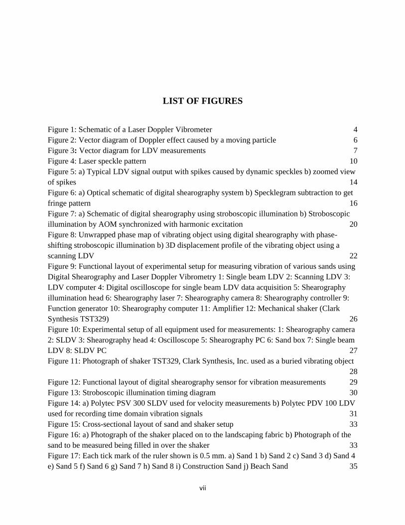
LIST OF FIGURES

Figure 1: Schematic of a Laser Doppler Vibrometer 4

Figure 2: Vector diagram of Doppler effect caused by a moving particle 6

Figure 3: Vector diagram for LDV measurements 7

Figure 4: Laser speckle pattern 10

Figure 5: a) Typical LDV signal output with spikes caused by dynamic speckles b) zoomed view

of spikes 14

Figure 6: a) Optical schematic of digital shearography system b) Specklegram subtraction to get

fringe pattern 16

Figure 7: a) Schematic of digital shearography using stroboscopic illumination b) Stroboscopic

illumination by AOM synchronized with harmonic excitation 20

Figure 8: Unwrapped phase map of vibrating object using digital shearography with phase-

shifting stroboscopic illumination b) 3D displacement profile of the vibrating object using a

scanning LDV 22

Figure 9: Functional layout of experimental setup for measuring vibration of various sands using

Digital Shearography and Laser Doppler Vibrometry 1: Single beam LDV 2: Scanning LDV 3:

LDV computer 4: Digital oscilloscope for single beam LDV data acquisition 5: Shearography

illumination head 6: Shearography laser 7: Shearography camera 8: Shearography controller 9:

Function generator 10: Shearography computer 11: Amplifier 12: Mechanical shaker (Clark

Synthesis TST329) 26

Figure 10: Experimental setup of all equipment used for measurements: 1: Shearography camera

2: SLDV 3: Shearography head 4: Oscilloscope 5: Shearography PC 6: Sand box 7: Single beam

LDV 8: SLDV PC 27

Figure 11: Photograph of shaker TST329, Clark Synthesis, Inc. used as a buried vibrating object

28

Figure 12: Functional layout of digital shearography sensor for vibration measurements 29

Figure 13: Stroboscopic illumination timing diagram 30

Figure 14: a) Polytec PSV 300 SLDV used for velocity measurements b) Polytec PDV 100 LDV

used for recording time domain vibration signals 31

Figure 15: Cross-sectional layout of sand and shaker setup 33

Figure 16: a) Photograph of the shaker placed on to the landscaping fabric b) Photograph of the

sand to be measured being filled in over the shaker 33

Figure 17: Each tick mark of the ruler shown is 0.5 mm. a) Sand 1 b) Sand 2 c) Sand 3 d) Sand 4

e) Sand 5 f) Sand 6 g) Sand 7 h) Sand 8 i) Construction Sand j) Beach Sand 35

viii

Figure 18: Shearography data a) Fringe pattern b) Filtered fringe pattern c) Unwrapped phase

map 36

Figure 19: Initial fringe deterioration caused by speckle decorrelation. a) Fringe pattern. b)

Filtered fringe pattern c) Unwrapped phase map 37

Figure 20: Shearograms (fringe pattern, filtered fringe pattern, and unwrapped phase map) for

sand 1 for different vibration amplitudes: a) 670nm b) 1.34μm c) 2.01μm d) 2.68μm e) 3.35μm f)

4.02μm g) 4.69μm h) 5.36μm 40

Figure 21: Displacement amplitude at which speckle decorrelation occurs vs grain size 42

Figure 22: a) Typical time domain signal from LDV for sand at low vibration amplitude b)

Zoomed in signal showing no spikes from dynamic speckle 45

Figure 23: a) Time domain signal from LDV for sand at high vibration amplitude b) Zoomed in

signal showing random bursts of spikes caused by dynamic speckles 45

Figure 24: PSD of LDV signal Sand 4 at 1mm/s velocity 46

Figure 25: Signal from sand #3 taken at 2mm/s velocity, at 2mm/s velocity the amplitude is so

low that the sand remains stable and doesn’t manifest any speckle noise 47

Figure 26: Signal from sand#3 taken at 12mm/s velocity, speckle noise results in frequent spikes

in the signal 47

Figure 27: Signal from sand#3 taken at 15mm/s velocity, at higher amplitude the spikes appear

more frequently throughout the waveform 48

Figure 28: Signal from sand#3 taken at 21mm/s, this is the highest amplitude achieved

throughout the measurements and the speckle noise is constant through the entire waveform 48

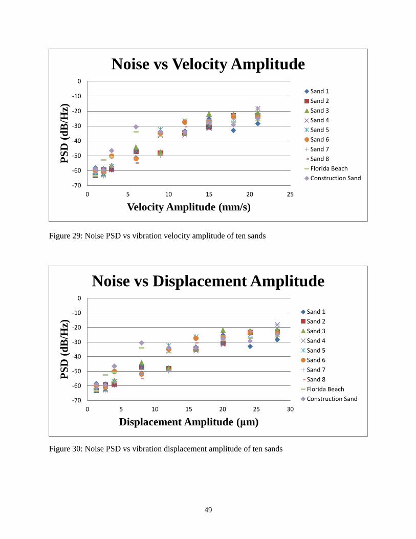
Figure 29: Noise PSD vs vibration velocity amplitude of ten sands 49

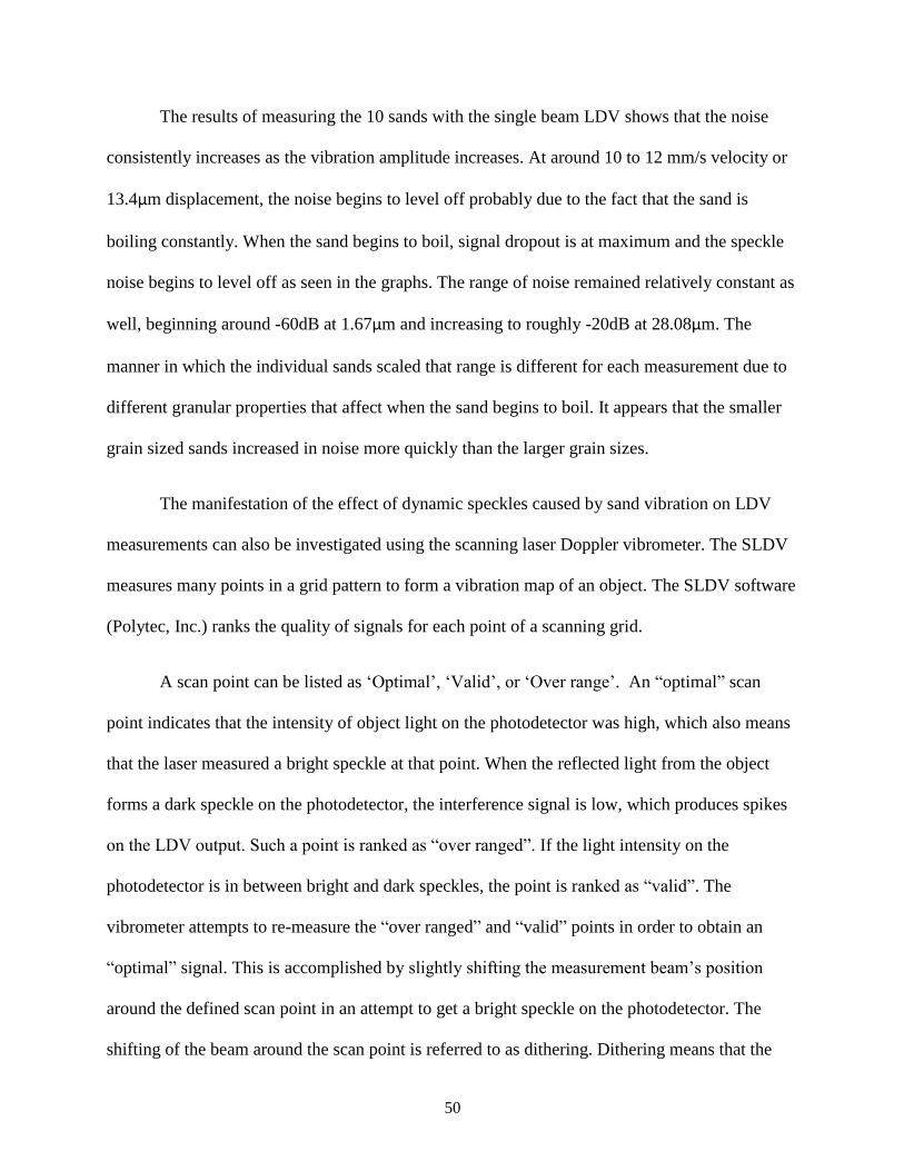
Figure 30: Noise PSD vs vibration displacement amplitude of ten sands 49

Figure 31: SLDV scan grid of sand above a buried shaker. Vibration amplitude was 500μm/s in

the area above the center of the shaker 52

Figure 32: SLDV scan grid of sand above a buried shaker. Vibration amplitude was 16mm/s in

the area above the center of the shaker. 52

1

I. INTRODUCTION

The use of interferometric sensors as non-contact vibration sensors such as the laser

Doppler vibrometer, electronic speckle pattern interferometer (ESPI), and digital speckle pattern

interferometer have become a popular choice for civil as well as military applications. These

sensors use the interference of coherent light incident on a surface to provide velocity and

displacement information. Interferometric sensors are very sensitive to small vibration

amplitudes making them suitable for precise non-contact measurements.

The LDV and electronic speckle pattern interferometers are non-contact vibration sensors

that are used in various lines of research on ground vibrations. The LDV measures point by point

and can develop a vibration map of the ground, whereas ESPI can measure whole fields of

interest simultaneously with high spatial resolution. Digital shearography sensors, similar to

ESPI, are less sensitive to platform motion than ESPI due to the lack of a reference beam. One

area of research for laser interferometric sensors is the detection of the vibration signatures of

landmines and other buried targets from a stand-off distance [1-11]. These sensors can detect

abnormalities in the vibration of the ground due to a buried object when ground is excited using

an acoustic or seismic source.

Publications have also investigated the LDV’s ability to passively detect underground

tunnels [12-13]. The LDV can detect the ground surface vibrations of activity within the tunnel

associated with humans’ movements or humans actively digging within the tunnel.

2

Another area of research for ground vibration measurements using LDVs is soil

characterization. The LDV can be used as a non-invasive measurement tool in lieu of more

invasive tools such as geophones for various soil characteristics such as ground water

measurements, moisture content, sound speed, subsurface soil layer measurements, and other

mechanical properties [14-18].

It has been observed that vibration of unconsolidated sand can affect the performance of

an interferometric sensor, due to the relative motion between soil particles [19]. The relative

motion of individual sand particles, caused by mechanical vibration, introduces noise in the

output of the LDV and causes speckle decorrelation in digital shearography sensors. The source

of this noise and decorrelation is variation in the laser speckle field caused by sand particle

motion. As sand particles move independently, speckles move - changing their intensity and

phase randomly and producing spikes in the demodulated output of these sensors.

The goal of this work is to investigate the effect of the vibration of various

unconsolidated sands on the performance of two interferometric techniques: laser Doppler

vibrometry and digital shearography. An overview of the basic principles of the laser Doppler

vibrometer and digital speckle pattern interferometer is presented in chapters 2 and 3. In chapter

4, the experimental work is presented along with the results of the experiments. In chapter 5,

conclusions are presented based on the results obtained.

3

II. BASIC PRINCIPLES OF LASER DOPPLER VIBROMETRY

A laser Doppler vibrometer is a precise optical sensor used to measure vibration velocity and the

displacement of an object. The principle of operation of the LDV utilizes the Doppler effect by

sensing the shift in frequency of coherent light scattered by a moving surface or object. Laser

Doppler vibrometers are well established non-contact sensors that provide greater flexibility than

the traditional contact vibration transducer. This section discusses the working principle of LDVs

and characteristics of LDV measurements associated with laser speckles.

4

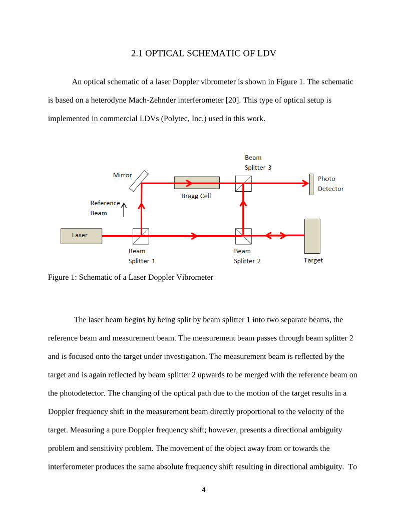
2.1 OPTICAL SCHEMATIC OF LDV

An optical schematic of a laser Doppler vibrometer is shown in Figure 1. The schematic

is based on a heterodyne Mach-Zehnder interferometer [20]. This type of optical setup is

implemented in commercial LDVs (Polytec, Inc.) used in this work.

The laser beam begins by being split by beam splitter 1 into two separate beams, the

reference beam and measurement beam. The measurement beam passes through beam splitter 2

and is focused onto the target under investigation. The measurement beam is reflected by the

target and is again reflected by beam splitter 2 upwards to be merged with the reference beam on

the photodetector. The changing of the optical path due to the motion of the target results in a

Doppler frequency shift in the measurement beam directly proportional to the velocity of the

target. Measuring a pure Doppler frequency shift; however, presents a directional ambiguity

problem and sensitivity problem. The movement of the object away from or towards the

interferometer produces the same absolute frequency shift resulting in directional ambiguity. To

Figure 1: Schematic of a Laser Doppler Vibrometer

5

combat the directional ambiguity issue as well as the sensitivity issue, the reference beam

undergoes a frequency shift. The reference beam is frequency shifted up or down by a certain

frequency, for example 40 MHz. This process is referred to as heterodyning, where the

frequency shift is provided by an acousto-optic modulator, also referred to as a Bragg Cell [21-

22]. Heterodyning affects the manner in which the signal beam and reference beam interfere with

one another. The frequency shift of the reference beam results in 40 MHz carrier frequency

signal on the photodetector. If the object is at rest, the interference of the measurement and

reference beams produces a 40 MHz carrier frequency signal on the photodetector. Using the

frequency shift allows measurement of absolute value and direction of the object velocity. If the

object moves towards or away from the interferometer, the resultant frequency will be more or

less than the carrier frequency allowing some directional sensibility. The introduction of the 40

MHz carrier frequency causes the reference beam and target beam frequency to cancel one

another out leaving only the beat frequency of 40 MHz.

6

2.2 THE DOPPLER EFFECT

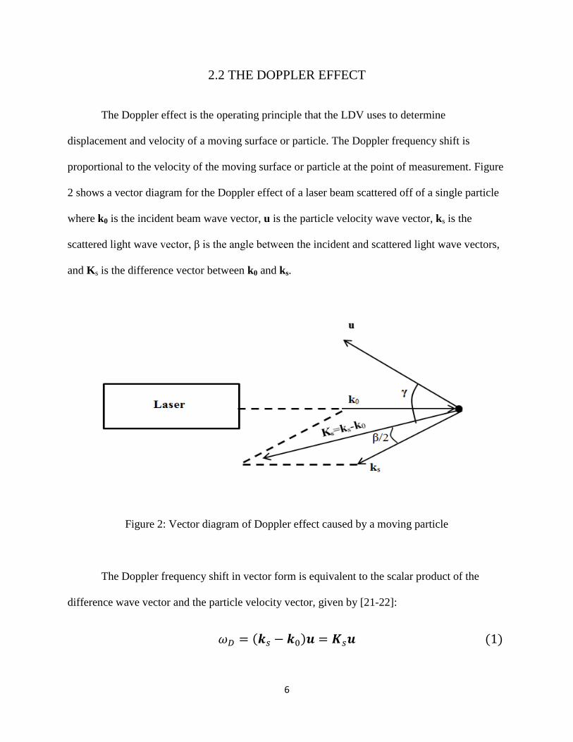
The Doppler effect is the operating principle that the LDV uses to determine

displacement and velocity of a moving surface or particle. The Doppler frequency shift is

proportional to the velocity of the moving surface or particle at the point of measurement. Figure

2 shows a vector diagram for the Doppler effect of a laser beam scattered off of a single particle

where k0 is the incident beam wave vector, u is the particle velocity wave vector, ks is the

scattered light wave vector, β is the angle between the incident and scattered light wave vectors,

and Ks is the difference vector between k0 and ks.

Figure 2: Vector diagram of Doppler effect caused by a moving particle

The Doppler frequency shift in vector form is equivalent to the scalar product of the

difference wave vector and the particle velocity vector, given by [21-22]:

𝜔𝐷 = (𝒌𝑠 − 𝒌0)𝒖 = 𝑲𝑠𝒖 (1)

7

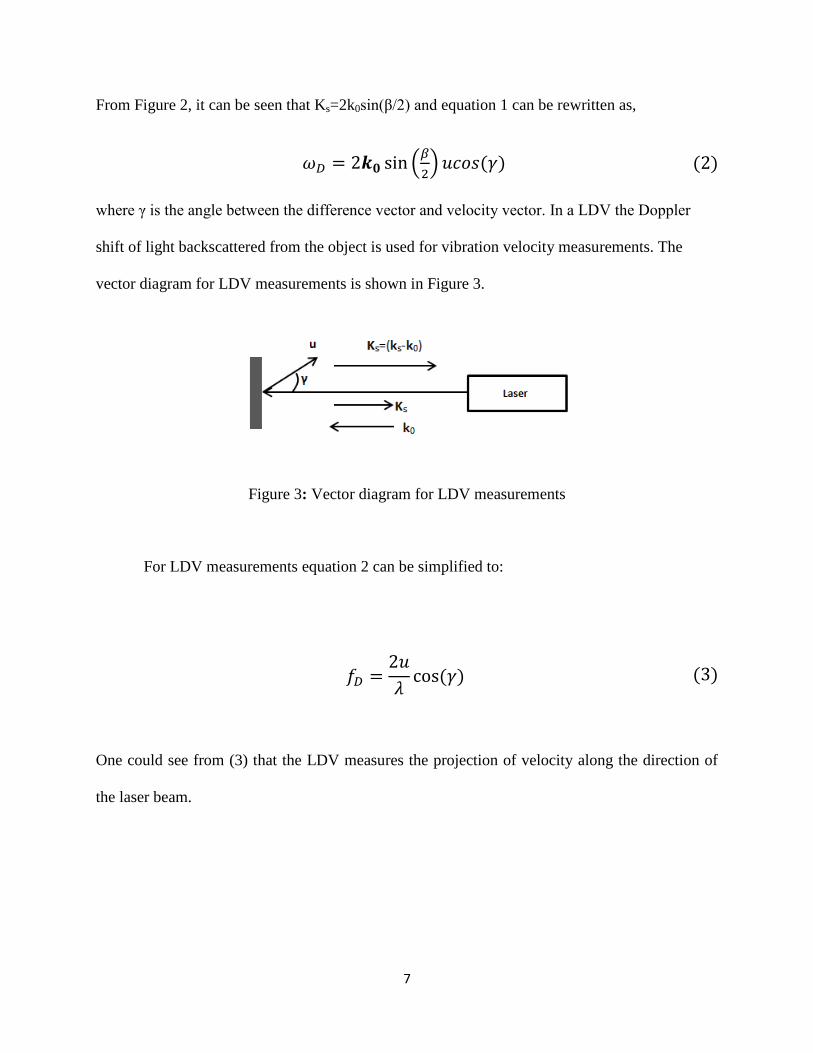
From Figure 2, it can be seen that Ks=2k0sin(β/2) and equation 1 can be rewritten as,

𝜔𝐷 = 2𝒌𝟎 sin (𝛽

2)𝑢𝑐𝑜𝑠(𝛾) (2)

where γ is the angle between the difference vector and velocity vector. In a LDV the Doppler

shift of light backscattered from the object is used for vibration velocity measurements. The

vector diagram for LDV measurements is shown in Figure 3.

Figure 3: Vector diagram for LDV measurements

For LDV measurements equation 2 can be simplified to:

𝑓𝐷 =

2𝑢

𝜆cos(𝛾) (3)

One could see from (3) that the LDV measures the projection of velocity along the direction of

the laser beam.

8

2.3 INTERFERENCE SIGNAL

At the interferometer output the light intensity resulting from the measurement beam and

reference beam interfering on the photodetector can be written as [5],

𝐼 = (𝐼𝑅 + 𝐼𝑆) + 2(𝐼𝑅𝐼𝑆)

1/2cos{[2𝜋𝑓𝐻𝑡 −4𝜋

𝜆𝑥(𝑡)] + (𝛷𝑅 −𝛷𝑆)} (4)

where IR and IS are the reference beam and target beam intensities, respectively, fH is the

heterodyning frequency, ΦR and ΦS are the phases of the reference beam and object beam

respectively on the photodetector, λ is the light wavelength, and x(t) is the target vibration

displacement. The DC component of the photodetector signal (IR+IS) presents little interest and is

usually filtered out before demodulation. The second term

𝐼𝐷 = 2(𝐼𝑅𝐼𝑆)

1/2 cos{ [2𝜋𝑓𝐻𝑡 −4𝜋

𝜆𝑥(𝑡)] + (𝛷𝑅 −𝛷𝑆)} (5)

is the Doppler signal that contains information on the vibration of the object. It is essentially a

frequency modulated signal with the carrier frequency fH. Demodulation of this signal reveals the

vibration velocity of the object. The amplitude and phase of the Doppler signal are random

values, due to interference of the reference wave with speckle field formed by diffuse reflection

of the laser beam from the rough surface of the object.

In some circumstances the Doppler signal amplitude can drop down to a low level

causing the carrier amplitude to become of the same order of magnitude as the LDV noise. When

9

this signal drop occurs, the demodulator cannot track the carrier signal and starts to track the

photodetector noise. The noise varies much quicker than the modulated signal, so the rapid

change results in sharp spikes. These spikes have a broad frequency range, making them difficult

to filter out of the signal and contribute to the velocity noise floor of the LDV.

Another source of noise is the variation of phase of the Doppler signal caused by

dynamic speckles. The carrier Doppler signal frequency fc can be expressed as the time

derivative of the cosine argument function from equation 5:

𝑓𝑐 = 𝑓𝐻 + 𝑓𝐷 +

1

2𝜋

𝑑𝛷𝑆(𝑡)

𝑑𝑡

(6)

The phase of the scattered light ΦS is dependent on time while the phase of the reference beam

ΦR does not change with time. When the speckle field does not change with time (i.e., dΦS/dt=0)

the frequency of the carrier Doppler signal simplifies to:

𝑓𝑐 = 𝑓𝐻 + 𝑓𝐷 (7)

When the speckle field varies, noise that corresponds to the frequency content of dΦS/dt appears

in the signal. This speckle noise is caused by variation of the phase of speckles. [24].

10

2.4 BASIC PROPERTIES OF LASER SPECKLES

When coherent light is incident on a surface where the surface roughness is on the scale

of the light wavelength, the scattered light wavelets become de-phased [25-26]. The component

wavelets interfere constructively and destructively resulting in a backscatter of high and low

intensities, also known as a speckle field. Laser speckles were first observed by Rigden and

Gordon in 1960 when operating the first continuous wave Helium-Neon laser [27]. A typical

laser speckle pattern is shown below in Figure 4.

The speckle pattern shown in Figure 4 shows the chaotic distribution of bright and dark

speckles. There are two types of speckles that occur - subjective and objective speckles.

Subjective speckles are produced at the image plane of a lens. They are caused by the

interference of waves from the various scattering regions of a resolution element of the lens. An

objective speckle pattern is formed in free space when a diffuse object is illuminated by coherent

light. The average size of objective speckles, also referred to as the space correlation function,

can be described as the distance between points where the intensity drops to one half of its

maximum value [28-29]. The average width bs of an objective speckle is given by [29]:

Figure 4: Laser speckle pattern

11

𝑏𝑠 ≅ 1.5𝜆 (

𝑍

𝐿) (8)

for a uniform intensity of the incident beam, where Z is the distance between the observed

speckle pattern and the diffuse surface and L is the width of the illuminated area of the diffuse

surface. If the object is illuminated with a Gaussian beam (as is the case for the LDV beam), the

average size of speckles formed in the diffraction field is given by:

𝑏𝑠 = λR/πw (9)

where λ is the wavelength of coherent light, R is the distance from the object to the observation

plane, and w is the radius of the Gaussian beam on the object [10]. For the subjective speckle in

the imaging plane, the average size is given by [28]:

𝑏𝑠 ≅ 1.22𝜆(

𝑍

𝐷) (10)

where D is the diameter of the lens. The intensity of the speckle pattern obeys negative

exponential statistics which states that it is far more likely for a dark speckle to appear than a

bright speckle. The probability density function for intensity is expressed by [28, 30-31],

𝑃𝐼(𝐼) =

𝐼

⟨𝐼⟩exp(−

𝐼

⟨𝐼⟩) (11)

12

where I and ‹I› is the intensity and the mean intensity of speckles respectively. The phase in

speckle pattern obeys uniform statistics, meaning that phase is a uniform distribution in the

interval of –π to π. The probability density function for phase is expressed by [30],

𝑃𝜃(𝜃) =

1

2𝜋𝑓𝑜𝑟 − 𝜋 ≤ 𝜃 < 𝜋 (12)

for any value of θ that is not -π≤θ<π, Pθ (θ)=0. A measure of the ratio of the standard deviation

of intensity, σI, to the mean intensity, I, is used to determine the contrast of the speckle pattern

[31-33],

𝐶 = 𝜎𝐼/⟨𝐼⟩ (13)

In general there are two types of dynamic speckle motions, translation and boiling. In

certain cases the diffuse object moves, causing the speckles to move but their shape remains

unchanged. This type of motion is referred to as ‘translation’ of the speckles. For other cases of

object motion or if the micro profile of the surface changes, individual speckles will deform,

disappear, and reappear without translation causing a temporally random variation of the speckle

field. This type of motion is referred to as ‘boiling’ of the speckles [29]. Speckle boiling is

focused on in this thesis, since the individual sand particles cause a change in the surface profile

therefore producing speckle boiling.

13

2.5 SPECKLE NOISE IN LDV

The variation of laser speckles introduces additional noise in the LDV; this noise is

referred to as speckle noise. This LDV noise is caused by the dynamic variation of speckles [29]

[34]. It has been shown that motion of an object, such as in-plane motion, rotation, and angular

motion, can increase the velocity noise floor due to speckle fluctuation. The scanning of a laser

beam across a surface also results in speckle noise due to speckles becoming dynamic. The

intensity and phase of dynamic speckles on the LDV photodetector change in a random way.

This variation results in random fluctuations of the amplitude and phase of the Doppler signal.

Since the intensity IS and the phase ΦS of the scattered light represent the intensity and phase of

the speckles respectively, the Doppler signal described by equation 5 is a random signal with

random amplitude and phase. When a laser beam is stationary relative to the object, the

amplitude and phase of the Doppler signal does not change with time. In the case where the

beam is stationary, the Doppler signal is spatially varying but not temporally varying. When the

object incurs angular or in-plane motion, or if the beam moves across the object, the speckles on

the photodetector vary, which results in a random variation of the Doppler signal amplitude and

phase. Random amplitude variation of the carrier Doppler signal occasionally causes dropouts of

the carrier signal down to a value comparable to the noise level in the photodetector. In that case,

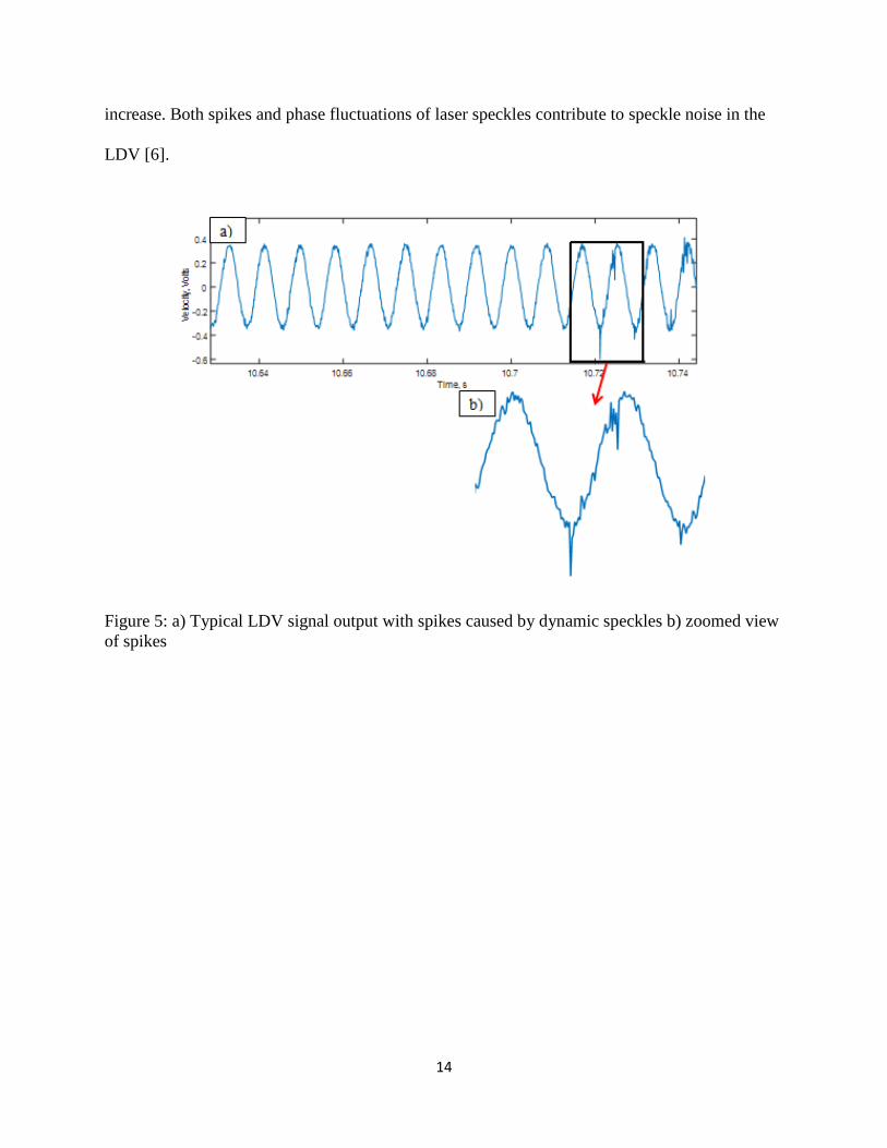
because of low signal, the FM demodulator can produce a spike in its output. Figure 5a shows an

example of spikes in the LDV signal caused by dropouts in the carrier signal due to dynamic

speckles. Figure 5b shows a zoomed in view of the spike. These spikes in the demodulated signal

have a broadband spectrum and they increase the velocity noise of the vibrometer. Phase

fluctuation of the Doppler signal due to dynamic laser speckles also causes the velocity noise to

14

increase. Both spikes and phase fluctuations of laser speckles contribute to speckle noise in the

LDV [6].

Figure 5: a) Typical LDV signal output with spikes caused by dynamic speckles b) zoomed view

of spikes

15

III. BASIC PRINCIPLES OF DIGITAL SHEAROGRAPHY

Digital shearography, also called digital speckle pattern shearing interferometry (DSPSI),

is a whole-field laser measuring technique based on shearing interferometry and digital data

processing. The technique is well-suited for nondestructive testing (NDT), strain measurements,

and vibration analysis [35-39]. Shearography is an interferometric measuring method that is

similar to electronic speckle-pattern interferometry (ESPI). However, shearography measures the

gradient of displacement of an object, not the displacement itself as ESPI does. Shearography is

simple in its optical setup, since the reference beam used in ESPI is not required. Because of the

lack of the reference beam, shearography has low sensitivity to platform motion and whole body

object motion. The other advantage of shearography is high spatial resolution of measurements;

depending on the number of pixels in the CCD or CMOS photodetector used, it can be better

than a millimeter for one square meter surface area. Sensitivity of digital shearography is /2 -

/4 in the real-time mode and /20-/30 when phase shifting interferometry is used ( is the

laser wavelength). This chapter will discuss the principles of DSPSI, the phase-shifting

technique, and speckle related issues with vibration measurements.

16

3.1 WORKING PRINCIPLE OF DIGITAL SHEAROGRAPHY

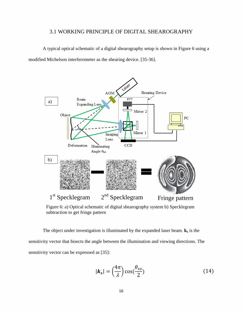
A typical optical schematic of a digital shearography setup is shown in Figure 6 using a

modified Michelson interferometer as the shearing device. [35-36].

The object under investigation is illuminated by the expanded laser beam. ks is the

sensitivity vector that bisects the angle between the illumination and viewing directions. The

sensitivity vector can be expressed as [35]:

|𝒌𝒔| = (

4𝜋

𝜆) cos(

𝜃𝑥𝑧2) (14)

Figure 6: a) Optical schematic of digital shearography system b) Specklegram

subtraction to get fringe pattern

1st Specklegram 2

nd Specklegram Fringe pattern

a)

b)

17

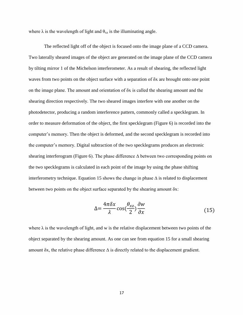
where λ is the wavelength of light and θxz is the illuminating angle.

The reflected light off of the object is focused onto the image plane of a CCD camera.

Two laterally sheared images of the object are generated on the image plane of the CCD camera

by tilting mirror 1 of the Michelson interferometer. As a result of shearing, the reflected light

waves from two points on the object surface with a separation of δx are brought onto one point

on the image plane. The amount and orientation of δx is called the shearing amount and the

shearing direction respectively. The two sheared images interfere with one another on the

photodetector, producing a random interference pattern, commonly called a specklegram. In

order to measure deformation of the object, the first specklegram (Figure 6) is recorded into the

computer’s memory. Then the object is deformed, and the second specklegram is recorded into

the computer’s memory. Digital subtraction of the two specklegrams produces an electronic

shearing interferogram (Figure 6). The phase difference ∆ between two corresponding points on

the two specklegrams is calculated in each point of the image by using the phase shifting

interferometry technique. Equation 15 shows the change in phase ∆ is related to displacement

between two points on the object surface separated by the shearing amount δx:

∆=

4𝜋𝛿𝑥

𝜆cos(

𝜃𝑥𝑧2)𝜕𝑤

𝜕𝑥

(15)

where λ is the wavelength of light, and w is the relative displacement between two points of the

object separated by the shearing amount. As one can see from equation 15 for a small shearing

amount δx, the relative phase difference ∆ is directly related to the displacement gradient.

18

3.2 PHASE-SHIFTING SHEAROGRAPHY

The numerical evaluation of a shearogram requires the determination of the relative phase

change difference ∆ for each point of measurement. To determine ∆, distributions of phase

difference φ of the first specklegram and φ’ of the second specklegram (φ’=φ+∆) are calculated

by using the phase shifting interferometry (PSI) technique. The relative phase difference ∆

before and after deformation can then be determined by subtracting φ from φ’. The phase

difference φ corresponds to the non-deformed state of the object. The phase difference φ’

corresponds to the deformed state of the object. These phase differences will be described as

phase distributions henceforth. Temporal phase shifting interferometry (PSI) is a common

technique to determine the phase distribution of an interferogram. By applying this phase-

shifting technique, shearograms can be evaluated quantitatively.

With the temporal PSI technique four interferograms of each deformation state of the

object are recorded sequentially in order to obtain a system of equations consisting of three

unknowns, intensities I1 and I2, and ∆. By slightly tilting mirror 1 of the Michelson

interferometer, two laterally sheared images of the object are produced. To generate the

additional phase needed for the PSI technique to work, mirror 2 of the Michelson interferometer

is driven by a piezoelectric transducer (PZT). The movement of mirror 2 controlled by the PZT

creates an additional phase φ. To generate an additional phase of π/2, mirror 2 must move by λ/8

for example. The intensity at each point of a specklegram can be expressed by:

𝐼 = 𝐼𝐴 + 𝐼𝐵 + 2√𝐼1𝐼2cos(∆)

(16)

19

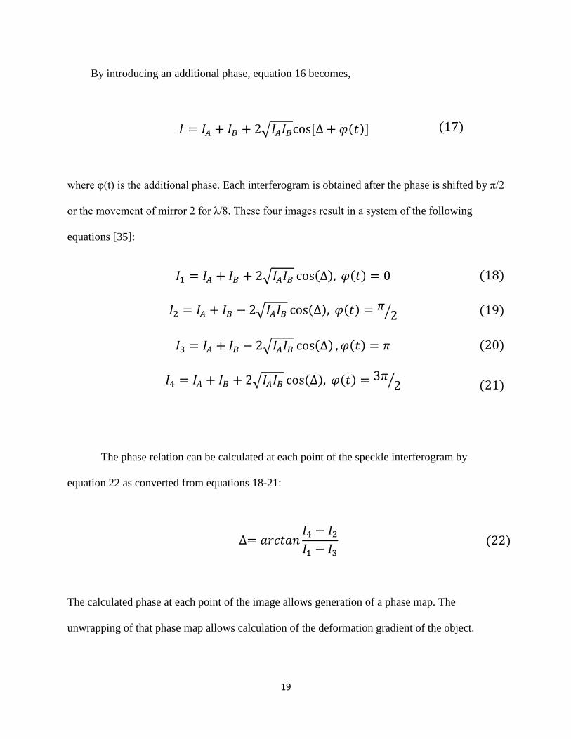
By introducing an additional phase, equation 16 becomes,

𝐼 = 𝐼𝐴 + 𝐼𝐵 + 2√𝐼𝐴𝐼𝐵cos[∆ + 𝜑(𝑡)]

(17)

where φ(t) is the additional phase. Each interferogram is obtained after the phase is shifted by π/2

or the movement of mirror 2 for λ/8. These four images result in a system of the following

equations [35]:

𝐼1 = 𝐼𝐴 + 𝐼𝐵 + 2√𝐼𝐴𝐼𝐵 cos(∆), 𝜑(𝑡) = 0 (18)

𝐼2 = 𝐼𝐴 + 𝐼𝐵 − 2√𝐼𝐴𝐼𝐵 cos(∆), 𝜑(𝑡) =𝜋2⁄ (19)

𝐼3 = 𝐼𝐴 + 𝐼𝐵 − 2√𝐼𝐴𝐼𝐵 cos(∆) , 𝜑(𝑡) = 𝜋 (20)

𝐼4 = 𝐼𝐴 + 𝐼𝐵 + 2√𝐼𝐴𝐼𝐵 cos(∆), 𝜑(𝑡) =3𝜋

2⁄ (21)

The phase relation can be calculated at each point of the speckle interferogram by

equation 22 as converted from equations 18-21:

The calculated phase at each point of the image allows generation of a phase map. The

unwrapping of that phase map allows calculation of the deformation gradient of the object.

∆= 𝑎𝑟𝑐𝑡𝑎𝑛

𝐼4 − 𝐼2𝐼1 − 𝐼3

(22)

20

3.3 VIBRATION MEASUREMENTS WITH DIGITAL SHEAROGRAPHY

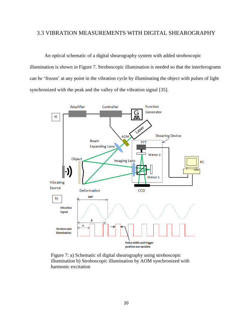
An optical schematic of a digital shearography system with added stroboscopic

illumination is shown in Figure 7. Stroboscopic illumination is needed so that the interferograms

can be ‘frozen’ at any point in the vibration cycle by illuminating the object with pulses of light

synchronized with the peak and the valley of the vibration signal [35].

Figure 7: a) Schematic of digital shearography using stroboscopic

illumination b) Stroboscopic illumination by AOM synchronized with

harmonic excitation

21

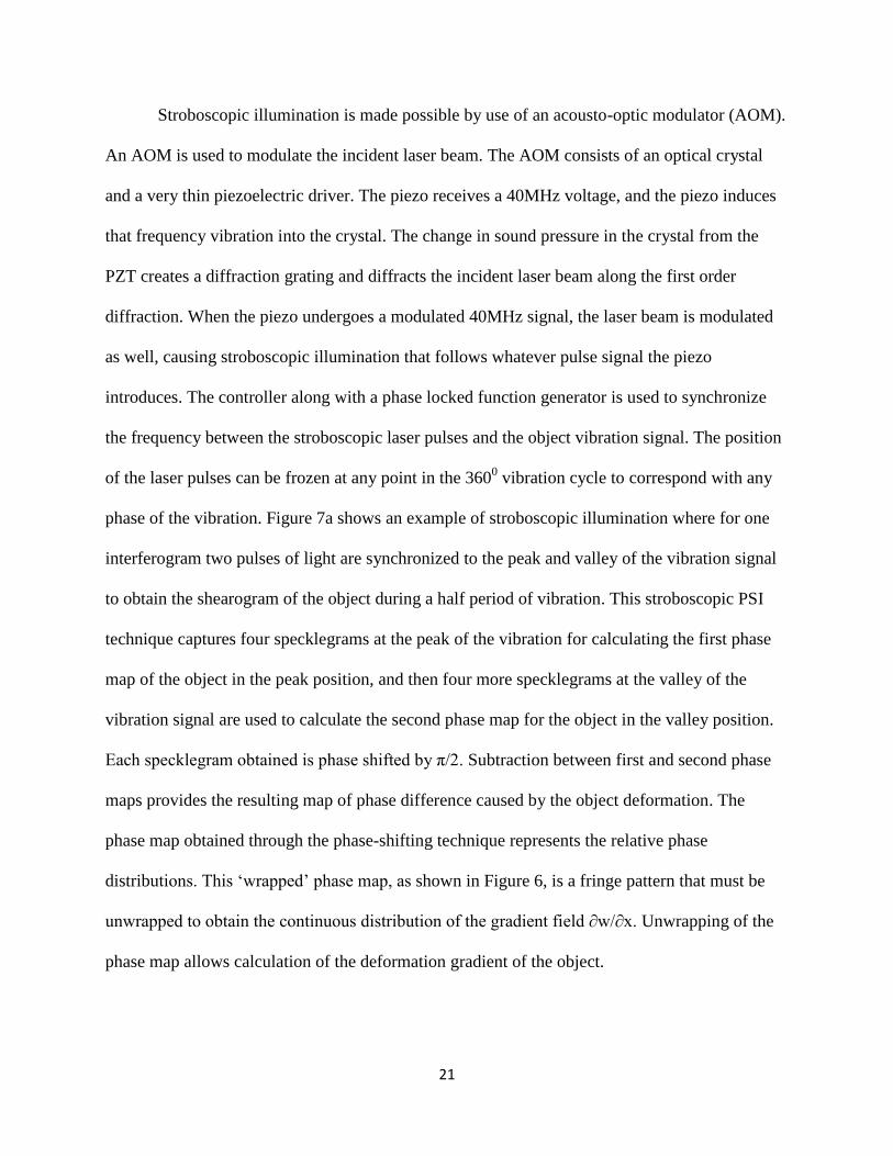
Stroboscopic illumination is made possible by use of an acousto-optic modulator (AOM).

An AOM is used to modulate the incident laser beam. The AOM consists of an optical crystal

and a very thin piezoelectric driver. The piezo receives a 40MHz voltage, and the piezo induces

that frequency vibration into the crystal. The change in sound pressure in the crystal from the

PZT creates a diffraction grating and diffracts the incident laser beam along the first order

diffraction. When the piezo undergoes a modulated 40MHz signal, the laser beam is modulated

as well, causing stroboscopic illumination that follows whatever pulse signal the piezo

introduces. The controller along with a phase locked function generator is used to synchronize

the frequency between the stroboscopic laser pulses and the object vibration signal. The position

of the laser pulses can be frozen at any point in the 3600 vibration cycle to correspond with any

phase of the vibration. Figure 7a shows an example of stroboscopic illumination where for one

interferogram two pulses of light are synchronized to the peak and valley of the vibration signal

to obtain the shearogram of the object during a half period of vibration. This stroboscopic PSI

technique captures four specklegrams at the peak of the vibration for calculating the first phase

map of the object in the peak position, and then four more specklegrams at the valley of the

vibration signal are used to calculate the second phase map for the object in the valley position.

Each specklegram obtained is phase shifted by π/2. Subtraction between first and second phase

maps provides the resulting map of phase difference caused by the object deformation. The

phase map obtained through the phase-shifting technique represents the relative phase

distributions. This ‘wrapped’ phase map, as shown in Figure 6, is a fringe pattern that must be

unwrapped to obtain the continuous distribution of the gradient field ∂w/∂x. Unwrapping of the

phase map allows calculation of the deformation gradient of the object.

22

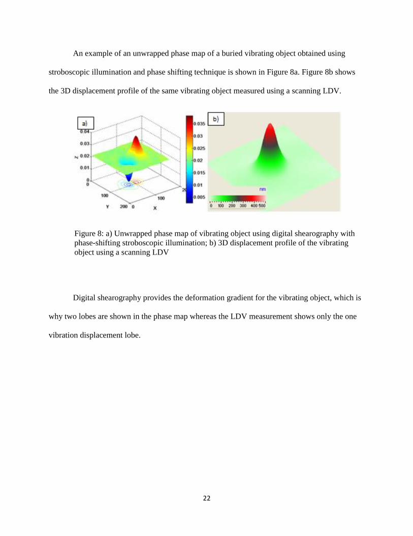
An example of an unwrapped phase map of a buried vibrating object obtained using

stroboscopic illumination and phase shifting technique is shown in Figure 8a. Figure 8b shows

the 3D displacement profile of the same vibrating object measured using a scanning LDV.

Digital shearography provides the deformation gradient for the vibrating object, which is

why two lobes are shown in the phase map whereas the LDV measurement shows only the one

vibration displacement lobe.

Figure 8: a) Unwrapped phase map of vibrating object using digital shearography with

phase-shifting stroboscopic illumination; b) 3D displacement profile of the vibrating

object using a scanning LDV

23

3.4 SPECKLE DECORRLEATION IN SPECKLE INTERFEROMETRY

One limitation of digital shearography, as well as ESPI, is speckle decorrelation. Digital

shearography requires the capture of and combining of two speckle patterns at two different

states of an object. In order to calculate an accurate phase distribution and produce a phase map,

the two speckle patterns must be correlated with one another. If the two speckle patterns do not

correlate with one another, then subtraction of the specklegrams will not yield any results as

contrast will be lost. Speckle decorrelation sets limitations on the amount of displacement an

object can incur during the measurement.

Speckle decorrelation can occur in several ways. An object can undergo in-plane motion,

tilt, or rotation that can cause the translation of the speckle pattern [38-39]. Deformation of an

object can also cause speckle decorrelation if it changes the structure of the object surface. Other

changes in the microscopic structure of an object surface can also result in speckle decorrelation.

When measuring solid objects, most speckle decorrelation occurs due to in-plane motion,

tilting, or rotation of the object. When the object is not solid, such as the case for measurements

on granular material such as sand, speckle decorrelation can be caused by the microscopic

change of the surface of the sand. When excited by vibration the particles of sand can change

their position relative to one another. As a result of this particle motion, the microscopic profile

of the sand surface changes and the speckles vary causing the correlation between two speckle

patterns obtained at different moments of time to be lost [19].

24

The effect of speckle decorrelation caused by vibration of dry sand is investigated in this

thesis. The goal is to experimentally investigate the effect of sand motion on vibration

measurements using laser Doppler vibrometry and digital shearography. The next chapter will

describe the experiments conducted and discuss the experimental results obtained.

25

IV. EXPERIMENTAL SETUP AND RESULTS

An experimental investigation of the effect of dynamic speckles caused by vibration of

unconsolidated sand on the performance of interferometric vibration sensors is conducted. The

performance of LDV and digital shearography is investigated. Both LDV and shearography are

used to measure vibration of dry sands with different grain sizes. Dependence of the LDV noise

on the amplitude of sand vibration is determined for different sand grain sizes. Digital

shearograms are also obtained for different vibration amplitudes for the same variety of sands, in

order to determine the vibration amplitudes causing interferogram deterioration.

26

4.1 EXPERIMENTAL SETUP

A functional layout of the experimental setup and a photograph of the setup are shown in

Figure 9 and 10, respectively.

Figure 9: Functional layout of experimental setup for measuring vibration of various

sands using Digital Shearography and Laser Doppler Vibrometry. 1: Single beam LDV.

2: Scanning LDV. 3: LDV computer. 4: Digital oscilloscope for single beam LDV data

acquisition. 5: Shearography illumination head. 6: Shearography laser. 7: Shearography

camera. 8: Shearography controller. 9: Function generator. 10: Shearography computer.

11: Amplifier. 12: Mechanical shaker (Clark Synthesis TST329).

27

Referencing Figure 10 the setup includes: single beam LDV (PDV100, Polytec Inc.),

scanning LDV (PSV300, Polytec Inc.), LDV computer, digital storage oscilloscope,

shearography illumination head, shearography laser, shearography camera, shearography

controller, function generator, shearography computer, amplifier, and shaker. From Figure 9, the

single beam LDV (1) is used to record time domain signals from the vibrating sand through use

of the digital storage oscilloscope (4). The scanning LDV (SLDV, 2) is used to measure the real-

time velocity amplitude of the vibrating sand for the purpose of incrementally stepping the

amplitude of vibration. Two LDV systems had to be used because there needed to be one LDV to

show the real-time velocity and another to record the time domain signals. The shearography

sensor includes the following components: laser, illumination head, shearography camera,

Figure 10: Experimental setup of all equipment used for measurements: 1:

Shearography camera. 2: SLDV. 3: Shearography head. 4: Oscilloscope. 5:

Shearography PC. 6: Sand box. 7: Single beam LDV. 8: SLDV PC.

28

controller, function generator, and computer. To provide a consistent source of vibration, a

shaker (Clark Synthesis, Inc. TST329, 12) was buried. The photograph of the shaker is shown in

Figure 11.The amplitude and frequency of vibration is controlled via a function generator (9)

33120A (HP) and amplifier (11) (Techron 5515). The shaker was excited at 119 Hz for these

experiments; this frequency was experimentally chosen because it produces an axisymmetric

vibration image.

Figure 11: Photograph of shaker TST329, Clark Synthesis, Inc. used as a

buried vibrating object

29

A functional layout of the digital shearography sensor used in these experiments is shown

in Figure 12.

This sensor was developed by Dr. Lianxiang Yang and his team at the Oakland

University Optical Metrology and Experimental Mechanics lab. The laser provides power to the

illumination head via a fiber optic cable and the controller. The laser used is a GLR-10 single

mode continuous wave 532nm fiber laser that features an optical head connected with a fiber

cable to an air-cooled rack-mounted laser power supply/controller; this laser is capable of 10

watt optical output (IPG Photonics). The surface of the sand is illuminated and the back reflected

light is captured by the camera. The sensor measures one square meter of the ground at a

Amplifier

Shaker

Function Generator 1 Function Generator 2

Controller

Laser

AOM

Piezo

Mirror

Shearography

Camera

CCD Detector

PC

Fiber

Target

Beam Expander

Beam

Splitter

Illumination Head

Figure 12: Functional layout of digital shearography sensor for vibration measurements

30

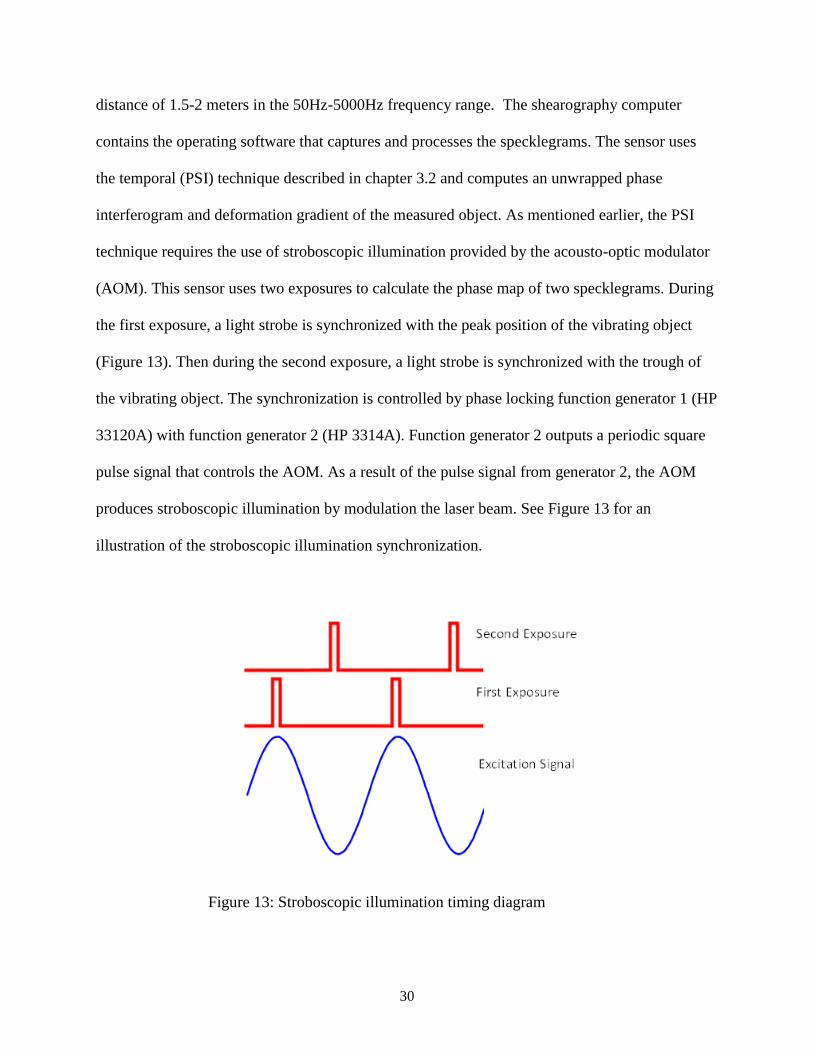
distance of 1.5-2 meters in the 50Hz-5000Hz frequency range. The shearography computer

contains the operating software that captures and processes the specklegrams. The sensor uses

the temporal (PSI) technique described in chapter 3.2 and computes an unwrapped phase

interferogram and deformation gradient of the measured object. As mentioned earlier, the PSI

technique requires the use of stroboscopic illumination provided by the acousto-optic modulator

(AOM). This sensor uses two exposures to calculate the phase map of two specklegrams. During

the first exposure, a light strobe is synchronized with the peak position of the vibrating object

(Figure 13). Then during the second exposure, a light strobe is synchronized with the trough of

the vibrating object. The synchronization is controlled by phase locking function generator 1 (HP

33120A) with function generator 2 (HP 3314A). Function generator 2 outputs a periodic square

pulse signal that controls the AOM. As a result of the pulse signal from generator 2, the AOM

produces stroboscopic illumination by modulation the laser beam. See Figure 13 for an

illustration of the stroboscopic illumination synchronization.

Figure 13: Stroboscopic illumination timing diagram

31

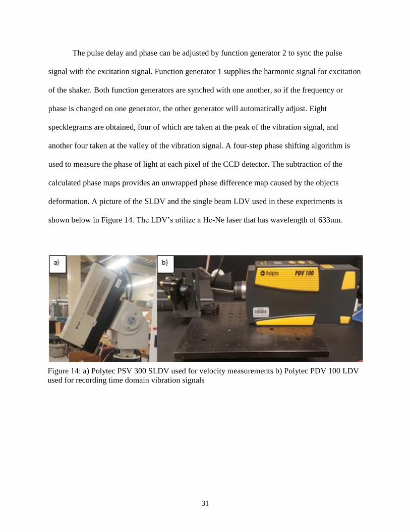
The pulse delay and phase can be adjusted by function generator 2 to sync the pulse

signal with the excitation signal. Function generator 1 supplies the harmonic signal for excitation

of the shaker. Both function generators are synched with one another, so if the frequency or

phase is changed on one generator, the other generator will automatically adjust. Eight

specklegrams are obtained, four of which are taken at the peak of the vibration signal, and

another four taken at the valley of the vibration signal. A four-step phase shifting algorithm is

used to measure the phase of light at each pixel of the CCD detector. The subtraction of the

calculated phase maps provides an unwrapped phase difference map caused by the objects

deformation. A picture of the SLDV and the single beam LDV used in these experiments is

shown below in Figure 14. The LDV’s utilize a He-Ne laser that has wavelength of 633nm.

Figure 14: a) Polytec PSV 300 SLDV used for velocity measurements b) Polytec PDV 100 LDV

used for recording time domain vibration signals

32

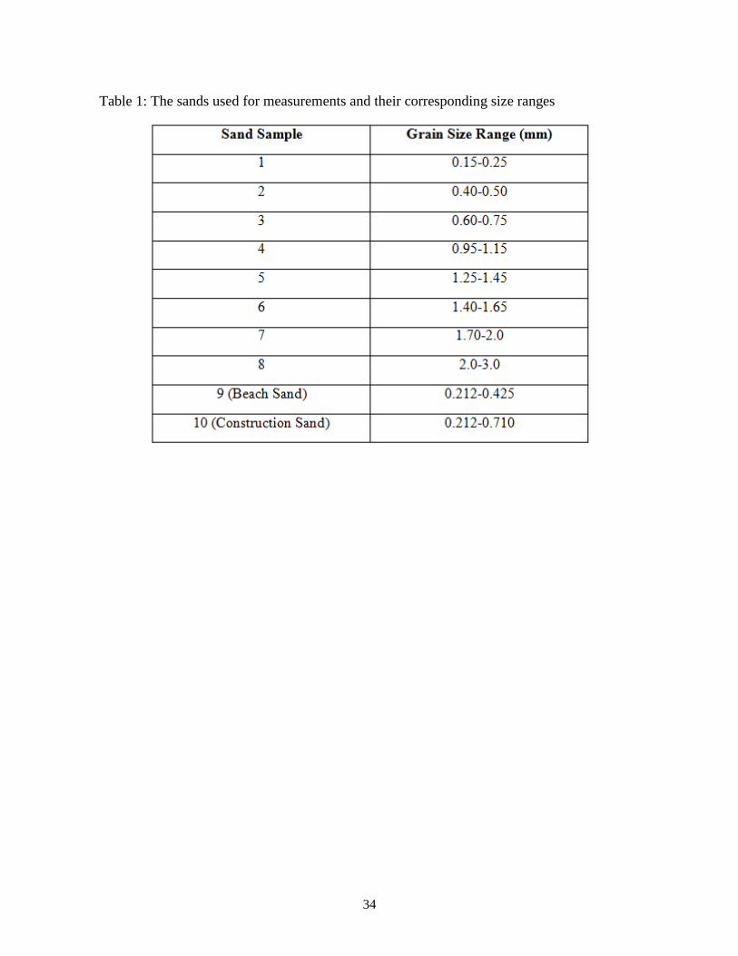
A total of 10 sands were used in the experiments. The sand samples and their grain size

distributions are listed in Table 1. A sieve analysis was performed for each sand to verify its size

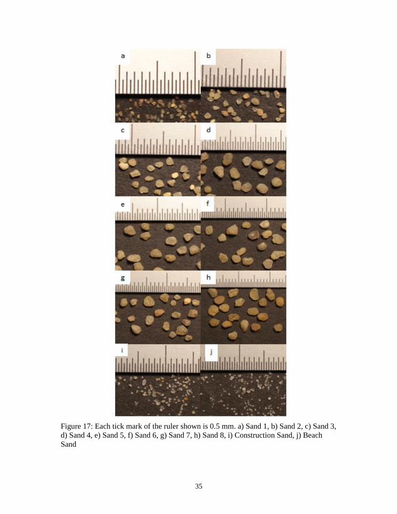
distribution. Figure 17 shows a photograph of the ten sands that are listed in Table 1. The

photograph helps to provide perspective about the size of the grains in each sample and show the

increase in grain diameter and grain shape.

Sands 1 through 8 are highly graded with narrow size distributions that begin with 150μm

and increase incrementally to 3.0mm grain diameter. The sand used in this work was graciously

donated by Premier Silica LLC in Colorado Springs, Colorado. The sand is comprised of almost

100% pure silica with a trace amount of aluminum oxide and potassium oxide present in the finer

grades of sand. A sample of sand from a Florida beach as well as construction sand were used to

serve as real world references. Collecting data on such a wide range of sand grain sizes allows

one to see a correlation between grain size and vibration amplitude that causes speckle

decorrelation. Dry, unconsolidated sand is inherently an unstable system; so to ensure accuracy

and repeatability, a strict experimental procedure was followed for each measurement.

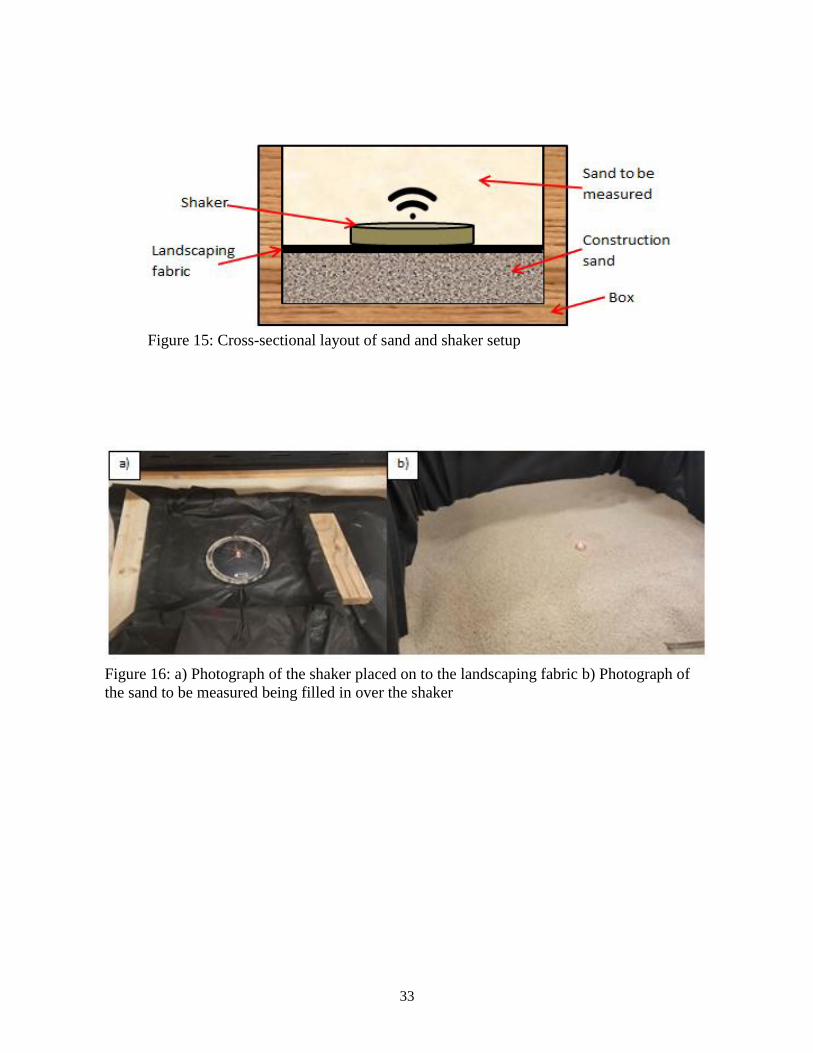
The first step was to fill the box with the sand to be measured, ensuring that the

mechanical shaker was buried at 3/4” depth (see Figures below). In Figures 15 and 16, the layout

that was used for the measurements is shown. Instead of using a large sandbox and having to

move large volumes of sand for every measurement, a small sand box was designed and built for

the measurements. Landscaping fabric was placed between some filler sand and the

measurement sand. The fabric makes changing the experiment quicker and prevents getting

samples mixed together. The shaker is placed onto the fabric and sand is then added.

33

Figure 15: Cross-sectional layout of sand and shaker setup

Figure 16: a) Photograph of the shaker placed on to the landscaping fabric b) Photograph of

the sand to be measured being filled in over the shaker

34

Table 1: The sands used for measurements and their corresponding size ranges

35

Figure 17: Each tick mark of the ruler shown is 0.5 mm. a) Sand 1, b) Sand 2, c) Sand 3,

d) Sand 4, e) Sand 5, f) Sand 6, g) Sand 7, h) Sand 8, i) Construction Sand, j) Beach

Sand

36

4.2 EXPERIMENTS ON SPECKLE DECORRELATION IN DIGTIAL

SHEAROGRAPHY

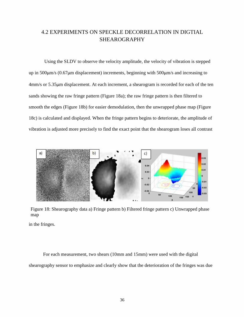
Using the SLDV to observe the velocity amplitude, the velocity of vibration is stepped

up in 500μm/s (0.67μm displacement) increments, beginning with 500μm/s and increasing to

4mm/s or 5.35μm displacement. At each increment, a shearogram is recorded for each of the ten

sands showing the raw fringe pattern (Figure 18a); the raw fringe pattern is then filtered to

smooth the edges (Figure 18b) for easier demodulation, then the unwrapped phase map (Figure

18c) is calculated and displayed. When the fringe pattern begins to deteriorate, the amplitude of

vibration is adjusted more precisely to find the exact point that the shearogram loses all contrast

in the fringes.

For each measurement, two shears (10mm and 15mm) were used with the digital

shearography sensor to emphasize and clearly show that the deterioration of the fringes was due

Figure 18: Shearography data a) Fringe pattern b) Filtered fringe pattern c) Unwrapped phase

map

37

to high vibration amplitude caused speckle decorrelation and not due to high fringe density since

lower shear produces less fringes.

Increasing the vibration amplitude of sand causes an increase in the number of fringes of

a shearogram. At the same time for some amplitudes, the fringe pattern begins to deteriorate.

This is the amplitude at which grains begin to move independently of one another, which causes

speckle decorrelation. That point, while sometimes hard to see with the raw image, becomes very

noticeable when the image is filtered. On the filtered fringe pattern, the discontinuities that cause

spikes in the unwrapped phase map are more apparent. An example of fringe deterioration

caused by speckle decorrelation is shown in Figure 19. One can clearly see from the Figure

below that the fringe lines at the center of the shearogram begin to merge together and become

discontinuous. These discontinuities cause the spikes in the unwrapped phase map in Figure 19c.

Figure 19: Initial fringe deterioration caused by speckle decorrelation. a) Fringe pattern. b)

Filtered fringe pattern c) Unwrapped phase map

38

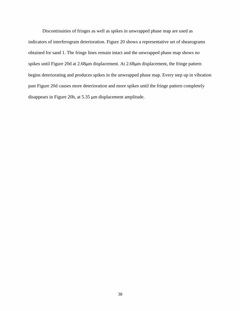
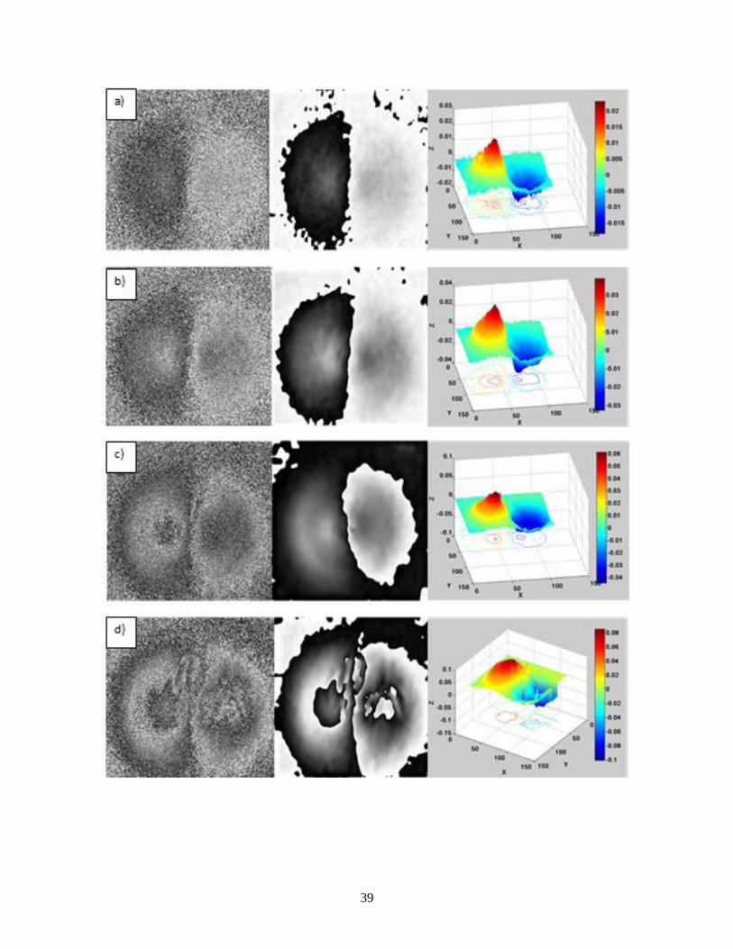
Discontinuities of fringes as well as spikes in unwrapped phase map are used as

indicators of interferogram deterioration. Figure 20 shows a representative set of shearograms

obtained for sand 1. The fringe lines remain intact and the unwrapped phase map shows no

spikes until Figure 20d at 2.68μm displacement. At 2.68μm displacement, the fringe pattern

begins deteriorating and produces spikes in the unwrapped phase map. Every step up in vibration

past Figure 20d causes more deterioration and more spikes until the fringe pattern completely

disappears in Figure 20h, at 5.35 μm displacement amplitude.

39

40

Figure 20: Shearograms (fringe pattern, filtered fringe pattern, and unwrapped phase map)

for sand 1 for different vibration amplitudes: a) 670nm b) 1.34μm c) 2.01μm d) 2.68μm e)

3.35μm f) 4.02μm g) 4.69μm h) 5.36μm

41

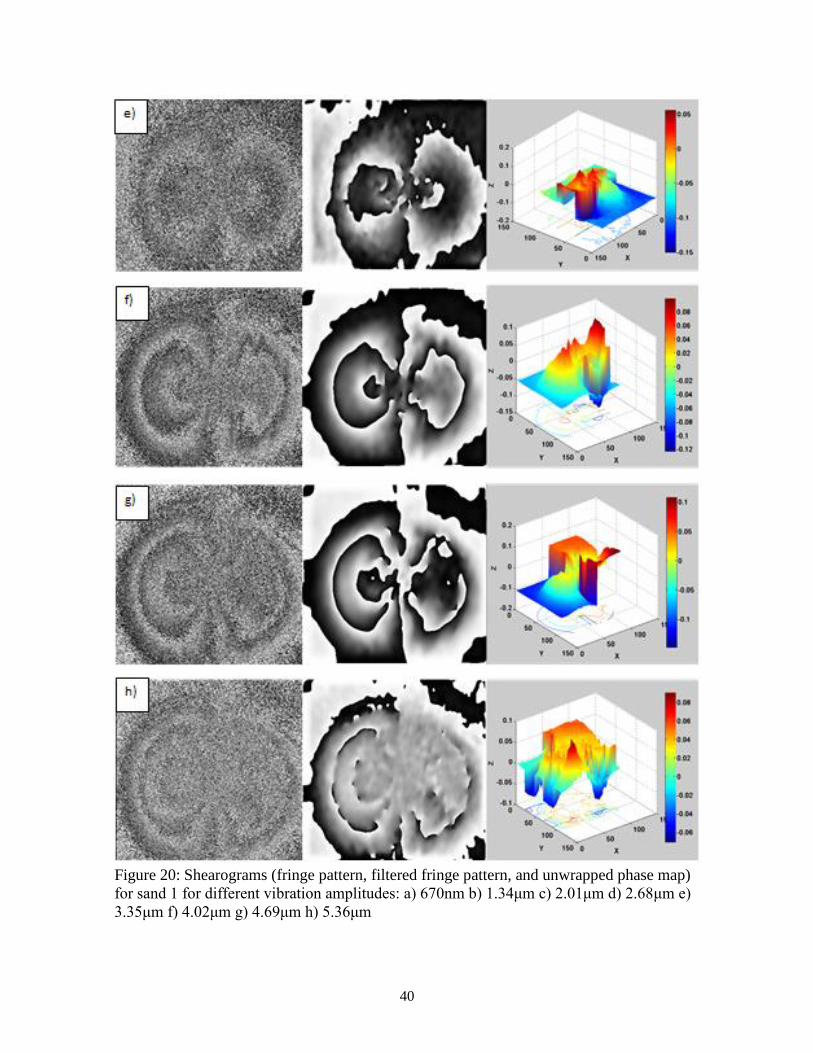
The measurement results for the ten sands are summarized in Table 2, showing the

vibration amplitude of the sand that causes speckle decorrelation and deterioration of

shearograms.

Table 2: Vibration amplitude of sand that causes speckle decorrelation

42

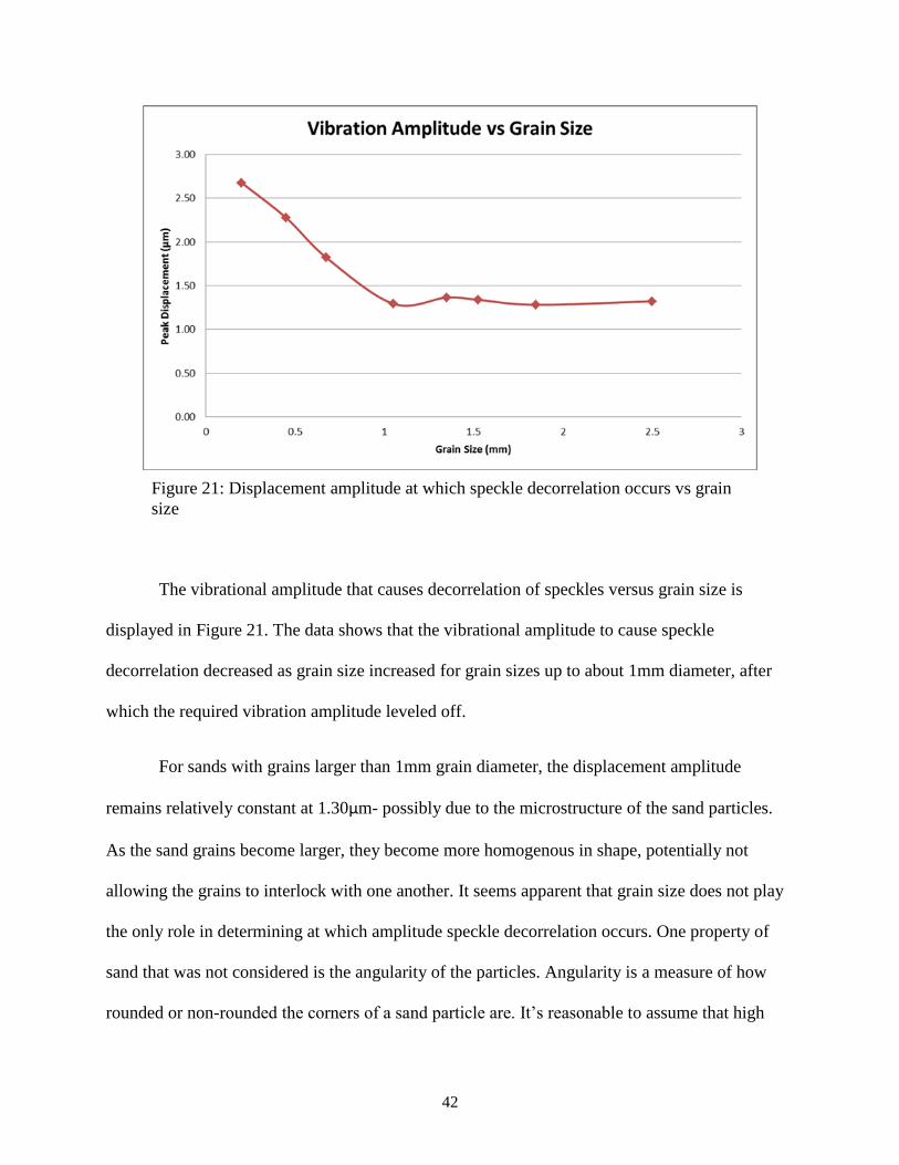
The vibrational amplitude that causes decorrelation of speckles versus grain size is

displayed in Figure 21. The data shows that the vibrational amplitude to cause speckle

decorrelation decreased as grain size increased for grain sizes up to about 1mm diameter, after

which the required vibration amplitude leveled off.

For sands with grains larger than 1mm grain diameter, the displacement amplitude

remains relatively constant at 1.30μm- possibly due to the microstructure of the sand particles.

As the sand grains become larger, they become more homogenous in shape, potentially not

allowing the grains to interlock with one another. It seems apparent that grain size does not play

the only role in determining at which amplitude speckle decorrelation occurs. One property of

sand that was not considered is the angularity of the particles. Angularity is a measure of how

rounded or non-rounded the corners of a sand particle are. It’s reasonable to assume that high

Figure 21: Displacement amplitude at which speckle decorrelation occurs vs grain

size

43

angularity (meaning sharp edges and non-uniform shape) could cause the sand to compact more

by locking together or forming cross-links between particles. This theory would explain why the

larger particles of sand (1mm and larger) did not change speckle decorrelation amplitude very

much. Referring back to Figure 17, it can be seen that the larger grain sizes appear more rounded

than the smaller grain sizes. This increased roundness means that there is less friction between

particles due to less contact surface area.

44

4.3 MEASUREMENTS OF LDV NOISE CAUSED BY VIBRATION OF

UNCONSOLIDATED SAND

Measurements to investigate how the LDV noise depends on the vibration amplitude of

unconsolidated sand uses the setup in Figures 15 and 16 with the single beam LDV placed above

the box attached to an optical rail (Figure 9 and 10). Time domain data was captured at 9

different vibration amplitudes, 1, 2, 3, 6, 9, 12, 15, 18 & 21mm/s velocities. When sand is

mechanically vibrated at relatively high amplitudes, the sand undergoes compaction affecting

subsequent measurements. Therefore, after every measurement the sand is perturbed to mitigate

compaction. This method was not used for digital shearography measurements because the

vibration amplitude used was much higher for the LDV measurements. Each time the sand is

perturbed, the optical signal strength of the LDV is verified to be optimal again to ensure there is

enough back-reflected light.

The LDV signal is recorded by using a Digital Storage Oscilloscope (Agilent Infiniium

54831B). The following acquisition parameters were used: sampling rate was 10,000 samples per

second, and the record length was 500,000 points, resulting in a 50 second long time domain

signal. A long recording time was desired to provide a better average for noise calculation. This

procedure was followed for all 10 samples of sand, and the LDV data was processed using a

Matlab code to calculate power spectral density of the LDV signal so that the noise could be

quantified. The Matlab codes used in this work were developed by Ina Aranchuk (National

Center for Physical Acoustics).

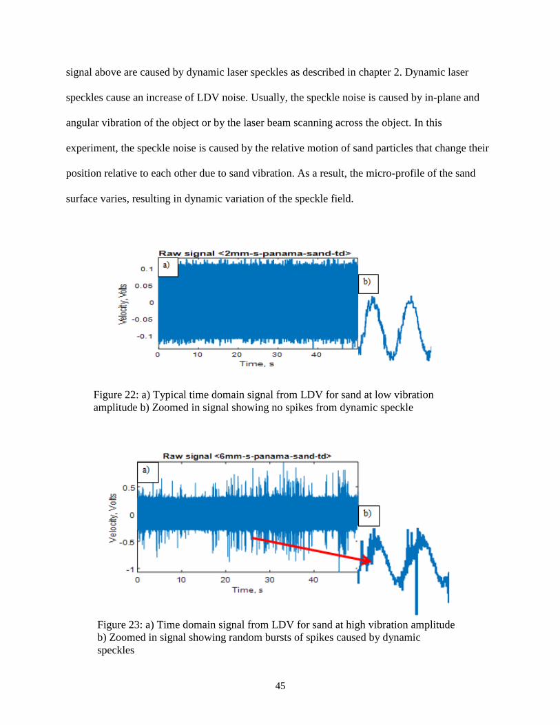
Figures 22 and 23 above serve as examples of what speckle noise looks like in a

waveform - it manifests itself as large spikes in LDV velocity signal. The spikes in the LDV

45

signal above are caused by dynamic laser speckles as described in chapter 2. Dynamic laser

speckles cause an increase of LDV noise. Usually, the speckle noise is caused by in-plane and

angular vibration of the object or by the laser beam scanning across the object. In this

experiment, the speckle noise is caused by the relative motion of sand particles that change their

position relative to each other due to sand vibration. As a result, the micro-profile of the sand

surface varies, resulting in dynamic variation of the speckle field.

Figure 23: a) Time domain signal from LDV for sand at high vibration amplitude

b) Zoomed in signal showing random bursts of spikes caused by dynamic

speckles

Figure 22: a) Typical time domain signal from LDV for sand at low vibration

amplitude b) Zoomed in signal showing no spikes from dynamic speckle

46

LDV noise was calculated in a 200Hz frequency band between 100Hz and 300Hz. This

frequency band presents the major interest for ground vibration sensing, for example for

detection of buried objects, and encompasses the signal frequency used of 119Hz. The noise was

calculated using power spectral density (PSD). PSD shows the average optical power distributed

as a function of frequency or the average noise power per unit bandwidth. PSD is expressed as

dB/Hz, so over some frequency band the average power in dB is calculated. An example of the

PSD calculated is shown below in Figure 24.

Figure 24: PSD of LDV signal Sand 4 at 1mm/s velocity

47

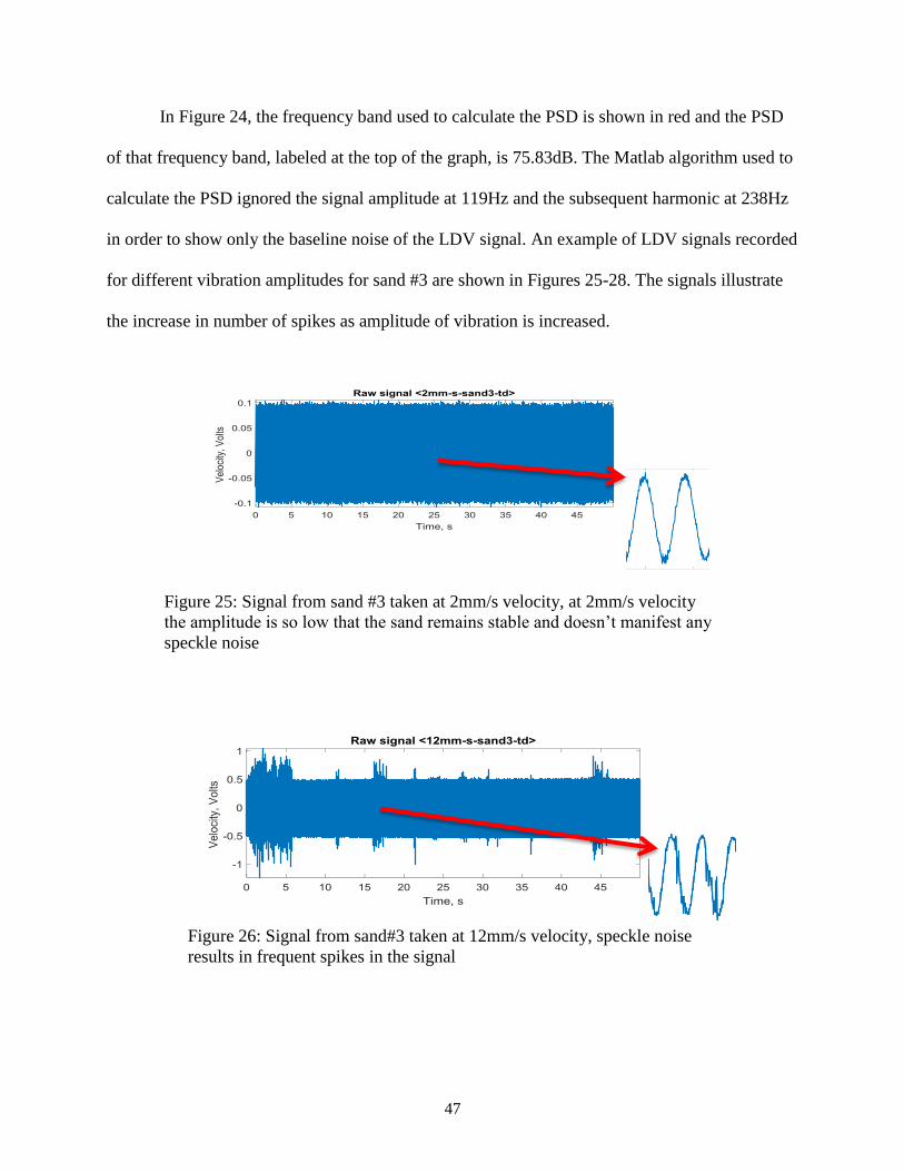
In Figure 24, the frequency band used to calculate the PSD is shown in red and the PSD

of that frequency band, labeled at the top of the graph, is 75.83dB. The Matlab algorithm used to

calculate the PSD ignored the signal amplitude at 119Hz and the subsequent harmonic at 238Hz

in order to show only the baseline noise of the LDV signal. An example of LDV signals recorded

for different vibration amplitudes for sand #3 are shown in Figures 25-28. The signals illustrate

the increase in number of spikes as amplitude of vibration is increased.

Figure 25: Signal from sand #3 taken at 2mm/s velocity, at 2mm/s velocity

the amplitude is so low that the sand remains stable and doesn’t manifest any

speckle noise

Figure 26: Signal from sand#3 taken at 12mm/s velocity, speckle noise

results in frequent spikes in the signal

48

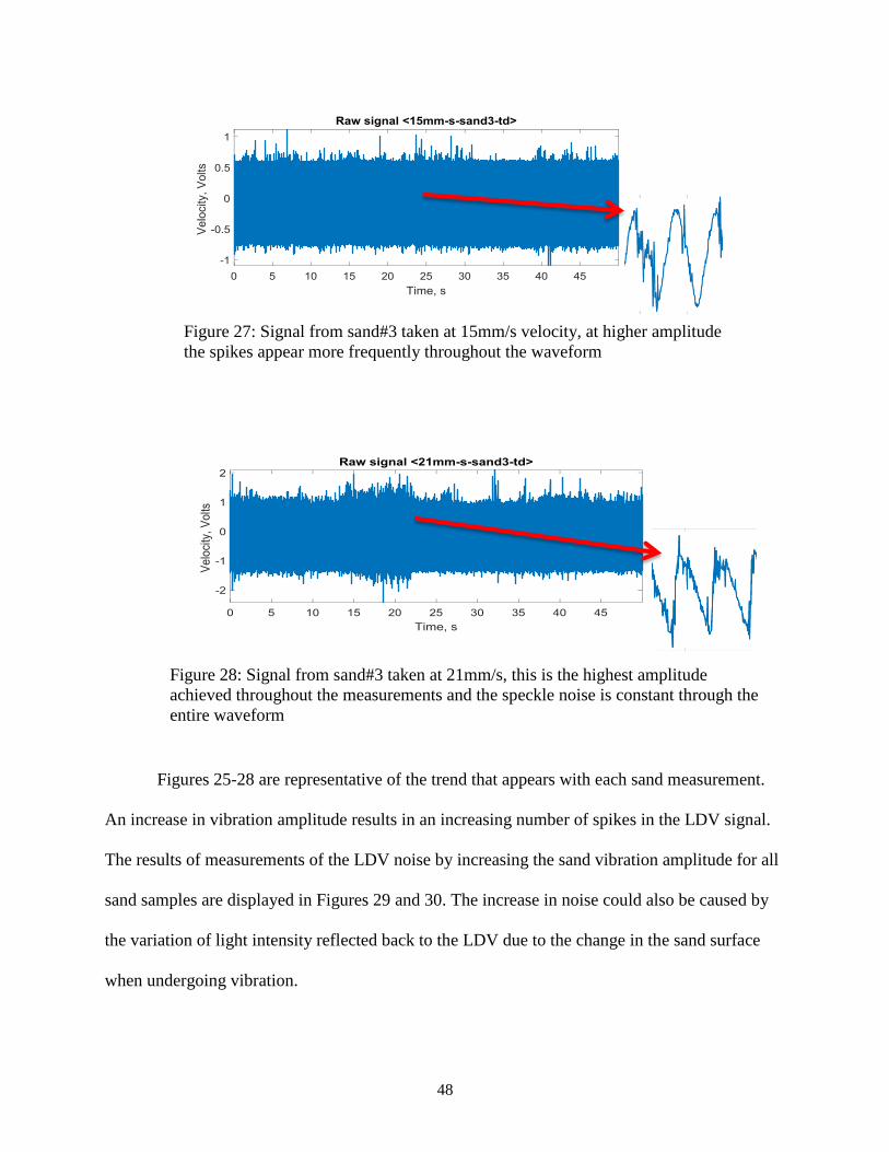
Figures 25-28 are representative of the trend that appears with each sand measurement.

An increase in vibration amplitude results in an increasing number of spikes in the LDV signal.

The results of measurements of the LDV noise by increasing the sand vibration amplitude for all

sand samples are displayed in Figures 29 and 30. The increase in noise could also be caused by

the variation of light intensity reflected back to the LDV due to the change in the sand surface

when undergoing vibration.

Figure 27: Signal from sand#3 taken at 15mm/s velocity, at higher amplitude

the spikes appear more frequently throughout the waveform

Figure 28: Signal from sand#3 taken at 21mm/s, this is the highest amplitude

achieved throughout the measurements and the speckle noise is constant through the

entire waveform

49

-70

-60

-50

-40

-30

-20

-10

0

0 5 10 15 20 25

PS

D (

dB

/Hz)

Velocity Amplitude (mm/s)

Noise vs Velocity Amplitude

Sand 1

Sand 2

Sand 3

Sand 4

Sand 5

Sand 6

Sand 7

Sand 8

Florida Beach

Construction Sand

-70

-60

-50

-40

-30

-20

-10

0

0 5 10 15 20 25 30

PS

D (

dB

/Hz)

Displacement Amplitude (μm)

Noise vs Displacement Amplitude

Sand 1

Sand 2

Sand 3

Sand 4

Sand 5

Sand 6

Sand 7

Sand 8

Florida Beach

Construction Sand

Figure 29: Noise PSD vs vibration velocity amplitude of ten sands

Figure 30: Noise PSD vs vibration displacement amplitude of ten sands

50

The results of measuring the 10 sands with the single beam LDV shows that the noise

consistently increases as the vibration amplitude increases. At around 10 to 12 mm/s velocity or

13.4μm displacement, the noise begins to level off probably due to the fact that the sand is

boiling constantly. When the sand begins to boil, signal dropout is at maximum and the speckle

noise begins to level off as seen in the graphs. The range of noise remained relatively constant as

well, beginning around -60dB at 1.67μm and increasing to roughly -20dB at 28.08μm. The

manner in which the individual sands scaled that range is different for each measurement due to

different granular properties that affect when the sand begins to boil. It appears that the smaller

grain sized sands increased in noise more quickly than the larger grain sizes.

The manifestation of the effect of dynamic speckles caused by sand vibration on LDV

measurements can also be investigated using the scanning laser Doppler vibrometer. The SLDV

measures many points in a grid pattern to form a vibration map of an object. The SLDV software

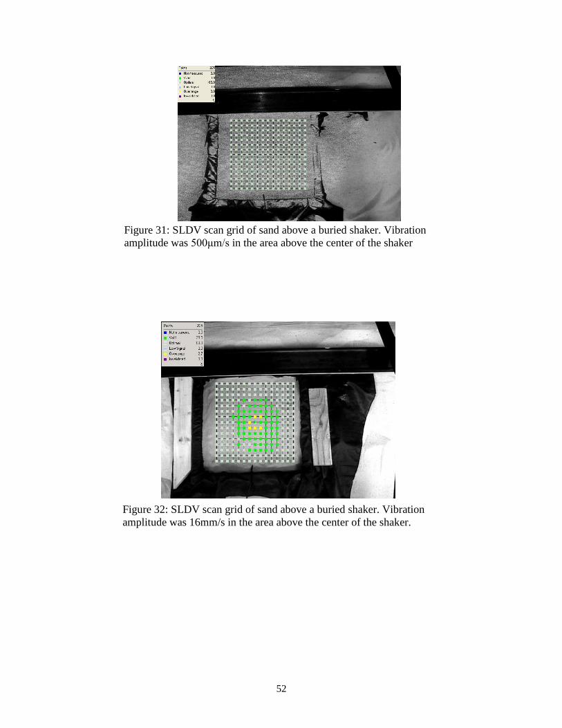
(Polytec, Inc.) ranks the quality of signals for each point of a scanning grid.

A scan point can be listed as ‘Optimal’, ‘Valid’, or ‘Over range’. An “optimal” scan

point indicates that the intensity of object light on the photodetector was high, which also means

that the laser measured a bright speckle at that point. When the reflected light from the object

forms a dark speckle on the photodetector, the interference signal is low, which produces spikes

on the LDV output. Such a point is ranked as “over ranged”. If the light intensity on the

photodetector is in between bright and dark speckles, the point is ranked as “valid”. The

vibrometer attempts to re-measure the “over ranged” and “valid” points in order to obtain an

“optimal” signal. This is accomplished by slightly shifting the measurement beam’s position

around the defined scan point in an attempt to get a bright speckle on the photodetector. The

shifting of the beam around the scan point is referred to as dithering. Dithering means that the

51

beam continuously ‘trembles’ around each scan point in order to measure a bright speckle. With

the amplitude of vibration high enough to cause the sand to boil and make the speckle field shift

continuously, the vibrometer will not be able to find a bright speckle in the time that the beam

has to measure the point. The system re-measures the scan points up to 10 times, attempting to

get a bright speckle, after which it stops scanning.

Figure 31 shows a grid of scanning points of sand surface above a buried vibrating

shaker. The maximum vibration velocity amplitude was 500μm/s in the area above the center of

the shaker. To obtain “optimal” status for all scan points, some of the points with initial “over

ranged” and “valid” status were re-scanned. Figure 32 shows the same grid of scanning points

for the vibration amplitude increased to 16mm/s in the area above the center of the shaker. One

can see that, despite the re-scanning attempts, the large area above the buried shaker shows

“valid” points, and several points in the center are “over ranged”. It means that the SLDV could

not find a beam position that would result in a bright speckle on the photodetector, because of

permanent variation of the speckle field. The higher amplitude in the center of the scan causes

large spikes in the signal that make some scanning points “over ranged”. Vibration of the area

with smaller amplitudes causes fewer spikes, making the scan points “valid”.

52

Figure 31: SLDV scan grid of sand above a buried shaker. Vibration

amplitude was 500μm/s in the area above the center of the shaker

Figure 32: SLDV scan grid of sand above a buried shaker. Vibration

amplitude was 16mm/s in the area above the center of the shaker.

53

V. CONCLUSIONS

The effect of vibration of unconsolidated dry sand on the performance of laser Doppler

vibrometry and digital shearography has been investigated experimentally for different grain size

sands. Eight highly graded sands with narrow size ranges between 0.15mm and 3.0mm, as well

as two real world sands, Florida beach sand and construction sand, have been used in the

experiments.

Vibration of dry sand can cause deterioration of a shearogram due to vibration-caused

speckle decorrelation. It has been found that the vibration amplitude of sand at which speckle

decorrelation in digital shearography occurs decreases from 2.68μm down to 1.30μm for the

increase of the sand grain size in the range from 0.15mm to 1 mm. For the sand grain sizes in

the range from 1 mm to 3mm, the vibration amplitude of sand at which speckle decorrelation

occurs doesn't depend on the grain size and is approximately 1.30μm. Vibration of

unconsolidated dry sand can increase the LDV noise. Dependence of the LDV noise power

spectral density (PSD) on the vibration amplitude has been obtained for sand grain sizes ranging

from 0.15 mm to 3mm. It was found that the LDV noise increases with the vibration amplitude

for amplitudes higher than approximately 2μm for all sands. The average increase in noise power

spectral density was found to be in the range from 34.2dB to 45.6dB for an increase in vibration

amplitude from 2μm to 22 μm.

54

The completed work shows that the effects of speckle variation caused by vibration of

unconsolidated granular materials, for example dry sand, and should be taken into account when

laser interferometric sensors are used for vibration measurements.

55

BIBLIOGRAPHY

56

BIBLIOGRAPHY

1. N. Xiang and J.M. Sabatier, “Land mine detection measurements using acoustic-to-

seismic coupling”, Proceedings of SPIE, Vol. 4038 pp. 645-655 (2000)

2. N. Xiang and J. M. Sabatier, “An experimental study on antipersonnel landmine detection

using acoustic-to-seismic coupling,” J. Acoust. Soc. Am. Vol. 113(3), pp. 1333–1341

(2003).

3. J.M. Sabatier, N. Xiang, A.G. Petculescu, V. Aranchuk, M. Bradley, and K. Murray,

“Vibration sensors for buried landmine detection”. Proceedings of International

Conference on Requirements and Technologies for the Detection, Removal, and

Neutralization of Landmines and UXO. September 2003, VUB, Brussels, Belgium pp.

483-488

4. A. K. Lal, H. Zhang, V. Aranchuk, E. Hurtado, C. F. Hess, R. D. Burgett, and J. M.

Sabatier, “Multiple-beam LDV system for buried landmine detection,” Proceedings of

SPIE, Vol. 5089 pp. 579-590 (2003)

5. J. M. Sabatier and V. Aranchuk, “An acoustic landmine detection confirmatory sensor

using continuously scanning multibeam LDV,” J. Acoust. Soc. Am. Vol. 115(5), p. 2416

(2004).

6. V. Aranchuk, A. Lal, C. Hess, and J.M. Sabatier, “Multi-beam laser Doppler vibrometer

for landmine detection”. Opt. Eng. Vol. 45(10), p. 104302 (2006).

7. R.W. Haupt, and K.D. Rolt, “Standoff acoustic laser technique to locate buried land

mines”. Lincoln Laboratory Journal Vol. 15(1), pp. 3-22 (2005).

8. J.C. van den Heuvel, V. Klein, P. Lutzmann, F.J.M, van Putten, H. Hebel, and H.M.A,

Schleijpen, “Sound wave and laser excitation for acousto-optical landmine detection”,

Proceedings of SPIE Vol. 5089 p. 569 (2003)

9. A.S. Turk, K.A. Hocaoglu, and A.A. Vertiy, Subsurface Sensing (John Wiley & Sons,

2011).

10. B. Saleh. (Ed.), Introduction to Subsurface Imaging (Cambridge University Press, 2011).

11. D.M. Donskoy, Resonance and Nonlinear Seismo-Acoustic Land Mine Detection

(INTECH Open Access Publisher, 2008).

12. J.M. Sabatier, and G.M. Matalkah, “A Study on the Passive Detection of Clandestine

Tunnels”, IEEE Conference on Technologies for Homeland Security, pp. 353-358

(2008)

13. P. Lutzmann, B. Göhler, F. Van Putten, and C.A. Hill, “Laser Vibration Sensing:

Overview and Applications”, International Society for Optics and Photonics, Vol. 818602

p. 818602 (2011).

14. Z. Lu, "Feasibility of Using a Seismic Surface Wave Method to Study Seasonal and

Weather Effects on Shallow Surface Soils", Journal of Environmental and Engineering

Geophysics Vol. 19(2) pp. 71-85 (2014).

57

15. Z. Lu, and J.M. Sabatier, "Effects of Soil Water Potential and Moisture Content on Sound

Speed", Soil Science Society of America Journal Vol. 73(5) pp. 1614-1625 (2009).

16. T. Sugimoto, Y. Nakagawa, T. Shirakawa, M. Sano, M. Ohaba, and S. Shibusawa, "Basic

Study on Water Distribution Measurement in Soil using SLDV", Ultrasonics Symposium

(IUS), IEEE International pp. 691-694 (2013).

17. N. Harrop and K. Attenborough, "Laser-Doppler Vibrometer Measurements of Acoustic-

to-Seismic Coupling in Unconsolidated Soils", Applied Acoustics Vol. 63(4) pp. 419-429

(2002).

18. D. Leary, D.A. DiCarlo, and C.J. Hickey, “Acoustic techniques for studying soil-surface

seals and crusts”, Ecohydrology Vol. 2(3) pp 257–262 (2009).

19. J.M. Sabatier, V. Aranchuk, and W.K. Alberts II, “Rapid High-Spatial-Resolution

Imaging of Buried Landmines using ESPI”, Proceedings of SPIE Vol. 5415 p. 15 (2004).

20. Measurement Solutions Made Possible by Laser Vibrometry. (2003). Retrieved January

15, 2017, from

http://www.polytec.com/fileadmin/user_uploads/Applications/Polytec_Tutorial/Documen

ts/LM_AN_INFO_0103_E_Tutorial_Vibrometry.pdf

21. L.E. Drain, The Laser Doppler Techniques (Chichester, Sussex, England and New York,

Wiley-Interscience, 1980).

22. C.B. Scruby, and L.E. Drain, Laser Ultrasonics Techniques and Applications (CRC

Press, 1990).

23. S. Rothberg, "Numerical Simulation of Speckle Noise in Laser Vibrometry." Applied

Optics Vol. 45(19) pp. 4523-4533 (2006).

24. V. Aranchuk, A.K. Lal, C.F. Hess, J.M. Sabatier, R.D. Burgett, I. Aranchuk, and W.T.

Mayo Jr, “Speckle Noise in a Continuously Scanning Multibeam Laser Doppler

Vibrometer for Acoustic Landmine Detection”, Proceedings of SPIE Vol. 6217 p. 621716

(2006)

25. S. Rothberg, and B.J. Halkon, “Laser Vibrometry Meets Laser Speckle”, Sixth

International Conference on Vibration Measurements by Laser Techniques: Advances

and Applications, Vol. 5503 p. 280 (2004).

26. J.D. Rigden and E. I. Gordon, "Granularity of Scattered Optical Maser Light",

Proceedings of the Institute of Radio Engineers Vol. 50(11) p. 2367 (1962).

27. C.M. Vest, Holographic Interferometry (John Wiley & Sons, 1979. pp. 66-69).

28. T. Asakura and N. Takai, "Dynamic Laser Speckles and Their Application to Velocity

Measurements of the Diffuse Object", Applied Physics A: Materials Science &

Processing, Vol. 25(3) pp. 179-194 (1981).

29. J.W. Goodman, "Statistical properties of laser speckle patterns." Laser speckle and

related phenomena (Springer Berlin Heidelberg, 1975. 9-75).

30. J.W. Goodman, Speckle Phenomena in Optics: Theory and Applications (Roberts and

Company Publishers, 2007).

58

31. J.D. Briers and S. Webster, "Laser Speckle Contrast Analysis (LASCA): A

Nonscanning, Full-Field Technique for Monitoring Capillary Blood Flow", Journal of

Biomedical Optics 1, pp. 174-179 (1996).

32. P. Martin and S. Rothberg, "Methods for the Quantification of Pseudo-Vibration

Sensitivities in Laser Vibrometry", Measurement Science and Technology, Vol. 22(3) p.

035302 (2011).

33. H.J. Rabal and R.A. Braga Jr, (Eds.), Dynamic Laser Speckle and Applications (CRC

Press, 2008).

34. S. Wolfgang and L. Yang, Digital shearography: Theory and Application of Digital

Speckle Pattern Shearing Interferometry (Bellingham: SPIE press, 2003).

35. L. Yang and X. Xie, Digital Shearography New Developments and Applications

(Bellingham: SPIE press, 2016.)

36. B. Bhaduri, N.K. Mohan, M.P. Kothiyal, and R.S. Sirohi, “Use of Spatial Phase Shifting

Technique in Digital Speckle Pattern Interferometry (DSPI) and Digital Shearography

(DS)” Optics Express, Vol. 14(24) pp. 11598-11607 (2006).

37. G. Cloud, Optical Methods of Engineering Analysis (Cambridge University Press, 1998).

38. I. Yamaguchi, "Speckle Displacement and Decorrelation in the Diffraction and Image

Fields for Small Object Deformation", Journal of Modern Optics, Vol. 28(10) pp. 1359-

1376 (1981).

59

VITA

Cody Scott Berrey_______________________________________________________________

EDUCATION

B.S, Mechanical Engineering, University of Mississippi, May 2015

EXPERIENCE

Sensors Engineer, Feb 2017 – present

General Atomics Electromagnetic Systems

Graduate Research Assistant, Aug 2015 – present

University of Mississippi, National Center for Physical Acoustics

Coherent Sensing Intern IV, June 2016 – Aug 2016

General Atomics Aeronautical Systems

Undergraduate Research Assistant, Aug 2013 – Aug 2015

University of Mississippi, National Center for Physical Acoustics