Effective conductivity of suspensions of hard spheres by...

Effective conductivity of suspensions of hard spheres by Brownian motion simulation

In Chan Kim Department of Mechanical and Aerospace Engineering, North Carolina State University, Raleigh, North Carolina 2769.57910

S. Torquato@ Department of Mechanical and Aerospace Engineering and Department of Chemical Engineering, North Carolina State University, Raleigh, North Carolina 27695 7910

(Received 9 August 1990; accepted for publication 8 November 1990)

A generalized Brownian motion simulation technique developed by Kim and Torquato [J. Appl. Phys. 68, 3892 ( 1990) ] is applied to compute “exactly” the effective conductivity a, of heterogeneous media composed of regular and random distributions of hard spheres of conductivity a, in a matrix of conductivity (pi for virtually the entire volume fraction range and for several values of the conductivity ratio a = ~~/a,, including superconducting spheres (a = CO ) and perfectly insulating spheres (a = 0). A key feature of the procedure is the use of

first-passage-time equations in the two homogeneous phases and at the two-phase interface. The method is shown to yield u, accurately with a comparatively fast execution time. The microstructure-sensitive analytical approximation of o, for dispersions derived by Torquato [J. Appl. Phys. 58,379O (1985) ] is shown to be in excellent agreement with our data for random suspensions for the wide range of conditions reported here.

I. INTRODUCTION The problem of determining the effective transport and

mechanical properties of multiphase media (given the phase properties and volume fractions) is an outstanding one in science and engineering. ‘,* Except for a few idealized models, there are no exact analytical predictions of the effective properties of random multiphase systems for arbitrary phase properties and volume fractions, even for the simplest class of problems, i.e., properties associated with transport processes governed by a steady-state diffusion equation (e.g., conductivity, dielectric constant, diffusion coefficient, trapping rate, etc.).2 For arbitrary phase properties and volume fractions, theoretical techniques basically fall into two cate- gories: effective-medium approximations3V4 and rigorous bounding techniques. ‘.‘-’ Comparatively, there is a dearth of work on the determination of effective properties from computer simulations, especially for continuum models (e.g., distributions of particles in a matrix). Such “computer experiments” could provide unambiguous tests on the afore- mentioned theories for well-defined continuum models.

Conventional approaches to obtaining o, by simulations solve the local governing differential equations for the fields (e.g., electric, temperature, concentration, etc.), subject to the appropriate boundary conditions at the multiphase interface of the computer-generated random heterogeneous system, using some numerical procedure such as finite differences, finite elements, or boundary elements. The solutions obtained for a sufficiently large number of such

;‘) Author to whom all correspondence should be addressed. Temporary ad- dress until May 31, 1991 is Courant Institute of Mathematical Sciences, New York University, 251 Mercer St., New York, NY 10012.

random configurations are then collected to yield the con- figurationally averaged fields and hence the effective properties. (For example, the effective electrical and thermal conductivities are defined by averaged Ohm’s and Fourier’s laws, respectively.) This is clearly a very wasteful way of obtaining the average behavior since there is a significant amount of information lost in going from the local to the average fields. It is not surprising, therefore, that such calculations become computationally exorbitant, even when per- formed on a supercomputer.

Recently, the authors8,9 have developed a Brownian motion simulation technique that directly yields the average behavior or effective properties of disordered n-phase heterogeneous media in which the transport process is governed by a steady-state diffusion equation

DV2Q> = - y (in each phase). (1) Here, @ is some potential, D is the diffusion coefficient, and y is a source term. The appropriate boundary conditions at the multiphase interface must be satisfied. Thus, for example, their algorithm can be applied to compute the effective conductivity (and mathematically analogous properties such as the dielectric constant, magnetic permeability, and diffusion coefficient) and the trapping rate associated with diffusion-controlled processes among static traps. Torquato and Kim” first applied the Brownian motion technique to compute the trapping rate by relating it to the inverse of the mean time taken for Brownian particles (representing the diffusing species) to get trapped. Kim and Torquato’ subse- quently extended the formulation to determine the effective conductivity of n-phase random media by relating it to the mean time associated with a Brownian trajectory in the limit of very large times. They specifically illustrated their meth-

2280 J. Appl. Phys. 69 (4), 1.5 February 1991 0021-8979/91/042280-i 0$03.00 @ 1991 American Institute of Physics 2280

Downloaded 12 Mar 2009 to 128.112.83.37. Redistribution subject to AIP license or copyright; see http://jap.aip.org/jap/copyright.jsp

od by obtaining a, for random arrays of infinitely long cylin- ders in a matrix.

Unlike recent random-walk algorithms which simulate the detailed zigzag motion of the walker with small finite steps,“‘-” the authors’ formulationsX~y utilize the appropri- atefirst-passage-time equations to compute mean times. Tor- quato and KimX demonstrated that in the trapping problem this results in an execution time that is at least an order of magnitude faster than the methods which simulate the detailed zigzag motion of the walker. The essence of the first- passage-time methodology is to construct the largest concentric sphere of radius R (around a randomly chosen initial location of the Brownian particIe) which just touches the multiphase interface. The mean time r taken for the Brow- nian particle (initially at the imaginary sphere center) to first strike a randomly chosen point on the sphere surface is simply proportional to R ‘. The process is repeated, each time keeping track of R ’ and thus r, until the walker comes within a small distance of the multiphase interface. At this juncture in the conduction problem, one must compute the mean time associated with crossing the boundary r,, and the probability of crossing the boundary, both of which depend upon the phase conductivities and local geometry, and were derived, for the first time, for arbitrary microstructures by Kim and Torquato’ using first-passage-time analysis. At some future time, the Brownian particle again will walk en- tirely in one phase and the above procedure is repeated. In the trapping problem, once the walker comes within a prescribed small distance of a trap, the walk is ended.

In this paper, we shall use Kim and Torquato’s generalized Brownian motion simulation technique to compute exactly the effective conductivity a, of a two-phase system composed of an equilibrium distribution of hard spheres of conductivity cr2 in a matrix of conductivity 0,. This is a useful model of a wide class of suspensions in which exclu- sion-volume effects play a dominant role in determining the microstructure. Conductivity data will be reported for virtually the entire volume fraction range and for a = o2 /a, = 0, 10, and CO. The data will then be compared to the approximate expression obtained by Torquato,13 which is expected to be highly accurate. Our data will be compared to previous results, including rigorous bounds.

Regular arrays of spheres are a useful theoretical bench- mark since the simplicity of such geometries permits exact solutions of 0,. Accordingly, we shall also determine o, for simple cubic lattices ofspheres and test these data against the exact results.

This paper is organized as follows. In Sec. II, we define the effective conductivity o‘, in terms of certain averages of the Brownian motion trajectories and present the appropriate first-passage-time relations that apply in the immediate vicinity of the boundary between two phases, say, phases 1 and 2. In Sec. III, we describe the simulation details to compute the effective conductivity a, for two-phase media composed of both simple cubic lattices and equilibrium distributions of hard spheres of conductivity (TV in a matrix of conductivity 0,. In Sec. IV, we report data for uI, and compare with previous results. In Sec. V, we make concluding re- marks.

II. BROWNIAN MOTION FORMULATION

The authors’ gave a general formulation to obtain exactly the effective conductivity a, for isotropic n-phase com- posites having phase conductivities 0, ,a,, . . . ,a,? in terms of certain averages of Brownian motion trajectories. To facili- tate the calculation they derived, for the first time, the appropriate first-passage-time equations which apply in the homogeneous phases and at the multiphase interface for d-dimensional media of arbitrary microstructure. Here, we shall apply our earlier general results to compute the effective conductivity of arbitrary three-dimensional distributions of spheres of conductivity o, in a matrix of conductivity 0,.

A. Effective conductivity

Consider a Brownian particle (conduction tracer) moving in a homogeneous spherical region R of conductivity o. Let the boundary be denoted by dR (see Fig. 1). The mean hitting time r(R), which is defined to be the mean time taken for a random walker initially at the center of a sphere of radius R and conductivity tz to hit the surface for the first time, is given by’

T(R) =R’. 6a

Equation (2) can be rewritten as

R2 g=-----. 67-(R)

(2)

(3)

Thus, if T(R), which represents the first hitting time averaged over an infinitely large number of such Brownian trajectories, is known, then the conductivity D can be obtained via Eq. (3). If an infinite medium is to be considered, the conductivity is given by

OAL.il ( 6T(R) IR--ra

. -I

The effective conductivity o, of an infinitely large composite medium can be computed in the same manner. Sup- pose we have a sphere of radius X which encompasses a distribution of spheres of conductivity c2 (phase 2) in a matrix (phase 1). If we view this sphere as an effective homoge-

dR

FIG. 1. Spherical homogeneous region R of conductivity o and radius R. Mean hitting time r = R l/60.

2281 J. Appl. Phys., Vol. 69, No. 4,15 February 1991 I. Chan Kim and S. Torquato 2281


FIG. 2. Circular region of radius Xcontaining a random suspension ofhard inclusions of conductivity e: in a matrix of conductivity 0,. The effective conductivity is (T,,. Brownian trajectory is schematically indicated, with R, denoting the first-passage-time radii.

neous sphere of conductivity a, (see Fig. 2), we can write in the spirit of Eq. (3) that

x2 ue = 67-,(x).

(5)

Here r, (X) is the total mean time associated with the total mean-square displacement X 2.

In the actual computer simulation, in most cases where the Brownian particle is far from the two-phase interface, we employ the same time-saving technique used by the author?.” which is now described. First, one constructs the largest imaginary concentric sphere of radius R around the diffusing particle which just touches the multiphase interface. The Brownian particle then jumps in one step to a random point on the surface of this imaginary concentric sphere, and the process is repeated, each time keeping track of R f (where R, is the radius of the ith first-passage sphere), until the particle is within some prescribed very small distance of two-phase interface. At this juncture, we need to compute not only the mean hitting time r, (R) associated with imaginary concentric sphere of radius R in the small neighborhood of the interface, but also the probability of crossing the interface. Both of these quantities, described fully below, are functions of o, ,02 and the local geometry. Thus, the expression for the effective conductivity used in practice is given by’

a, = G,R f + E]Rf + Z,R :>

6(2,~, (Rt ) + Ejr2 (RI 1 + zkr, (R, 1) ’ (6)

since X2=(2,Rf+Z,R~+2,,R:). Here, 7, (RI [ r2 (R) ] denotes the time for a random walker to make a first flight in a homogeneous sphere of radius R of conductivity 0, ( o2 ), the summations over the subscript i andj are for the random-walk paths in phase 1 and phase 2, respectively, and the summation over the subscript k is for the random-walk paths crossing the interface boundary.

Since each path segment, having mean-square displacement R f or R J’, is wholly contained in an homogeneous part

of the medium, Eqs. (2) and (6) yield

ff, = (ZiRf+E,RJ+B,Ri) 6@,Rf/60, + E,R,%u, + Z,r,(Rk))

or

ue -= (Z,Rfi~l + zjRf/U, +I;,R:/o,) 0' (ZiRf/a, +x,Rj/~, +62,r,(R,)) ' ('I

Each term inside the brackets of Eq. (8 ) has dimensions of time, and therefore (8) can be rewritten as

ffe -= (Tr, CR;) + xjr, (Rj) + 2,r, CR, )> UI (2;7,(R,) +xjrl(R,)/a+ C,r,(R,)) ' (9)

Here a = a, /a, is the conductivity ratio. If an infinite medium is to be considered, then we have

0, -= (z,r, (R,) + zjr, (Rj) + Z,r,(R,)) Cl (Girl +~jr,(Rj)/a+8,r,(R~)) X--m.

(10)

Note that, for an infinite medium, the initial position of the Brownian particle is arbitrary. Equation (IO) is the basic equation used to compute the effective conductivity.

B. Random walk crossing the interface boundary Here, we employ the appropriate first-passage-time

equations’ (i.e., mean hitting times and probabilities) which apply in a very small neighborhood of the generally curved interface boundary (see Fig. 3). The basic questions are (i) What is the probability p, (x) [p2 (x)] that the random walker initially at x near h, the center of an imaginary sphere of radius R, hits the surface in phase 1, JR, (the surface in phase 2, da2 ) for the first time without hitting Js1, (JR, )? (ii) What is the mean hitting timers (x) for the random walker initially at x to hit dR ( = da, UCTC& ) for the first time? Note that the initial position of the random walker is generally not at the interface.

_.-- . . . . : . .

R, ---*..* .

,

,

0 ‘. an, .

FIG. 3. Two-dimensional depiction of the small neighborhood of the curved interface boundary between phase 1 of conductivity o, and phase 2 of conductivity oJ.

2282 J. Appl. Phys., Vol. 69, No. 4, 15 February 1991 I. Chan Kim and S. Torquato 2282


First-passage-time analysis leads to the boundary-value problems given by9

vp, = 0, in 0 (=Ck,lJfl,),

p, (xl = 1, on Xl,,

p,(x) =o, on X&,

PI (x)l, =p, (x)l,, on r, (11)

21, =a-$$l,, on l?,

p2 (xl = 1 -p, (xl, a,v21-, = - 1, in C!; (i= 1,2),

Q-, (xl = 0, on &A,

r,(x)I, = T$(X)IZ, on r,

$1, =a$-12, on r.

(12)

(13)

Here r denotes the interface surface, n, denotes unit outward normal from region R,, and ( a) Ii means the approach to f from the region R, (i= 1,2). Note that the imaginary sphere of radius R described above is centered on the interface boundary rather than on the random walker since the former lends itself to a more tractable solution.

The solutions of Eqs. ( 1 1 )-( 13) for an interface with an infinite radius of curvature (straight line for d = 2 or plane for d = 3) is straightforward and for d>2 is given by an infinite series involving d-dimensional spherical harmon- ics.’ We seek, however, a solution for curved interfaces since this will result in more accurate calculations and because the radius R in practice does not have to be as small as it would have to be in the zero-curvature case, thus reducing the computation time. The general solution is intractable analytical- ly, but we have devised an approximate analytical solution’ (based upon the zero-curvature solution) which turns out to give excellent agreement with a numerical evaluations of Eqs. ( 1 l)-( 13). These general solutions are given by the following relations:

p,tr,m = Al

A, +aA, 1+a 2 B2,n+I

,n = 0

for O<r<R, oaXd2,

p,(rJa = Al

A, +aA, 1 + 2 Bz,,, + I

tn = 0

2in+ I P 2,n + I (cos 0) 9 1

for O<r<R, r/2<0<n, where

B ( - 1)‘“(2m)! 4m + 3 2’n L ’ = 22m+l(m!)2 Z’

p2 (r,B) = 1 -pI h%,

for O<r<R, O<fkn,

2283 J. Appl. Phys., Vol. 69, No. 4,15 February 1991

(14a)

(14b)

(15)

R 2 v’, + v* rs (r,O) = - 60, V, +aV,

x P*(cos 0) FG(r,B) , 1 for O<r<R, OQ<r/2,

R2 7,(r,f3) = - v, + v,

6~7, V, +aV,

x P,(COS 0) G(r,Q) , 1 (16)

for O<r<R, r/2<tkr, where

G(r,@ = g C2,,,+, + 0

2m + I

Cm+, (coW, m = 0

C (- 1) “I+ ‘(2m)! 3(4m + 3) 2mtl = 2’” + ‘(m!)2 (2m - l)(m + 2)(m + 1) .

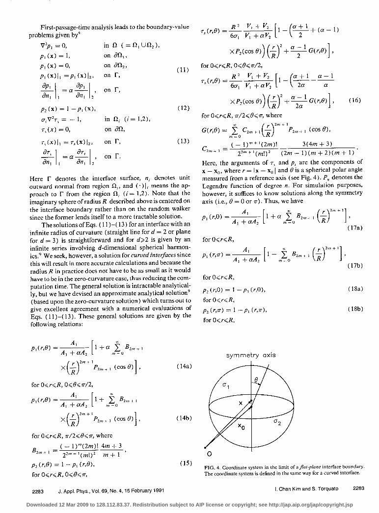
Here, the arguments of r, and p, are the components of x - x0, where r = Ix - x0 1 and 8 is a spherical polar angle measured from a reference axis (see Fig. 4). P, denotes the Legendre function of degree n. For simulation purposes, however, it suffices to know solutions along the symmetry axis (i.e., 8 = 0 or r). Thus, we have

pl (r,O) = Al

A, +aA, (17a) for O<r<R,

Al l-+2,,+, +

*tn+ I

p, O-+-l = A, +aA, 0 I

p ,n = 0

(17b)

for O<r<R,

p2 (r,O) = 1 -pI (r,O), for O<r<R,

(18a)

p2 (r,v) = 1 -p, (r,n), for O<r<R,

(18b)

symmetry axis

FIG. 4. Coordinate system in the limit of ajar-plane interface boundary. The coordinate system is defined in the same way for a curved interface.

I. Chan Kim and S. Torquato 2283


(19a)

for O<r<R,

(19b) for O<r<R, where

B ( - 1)‘“(2m)! 4m + 3 2rnfI = 2 2m+‘(m!)2 m+l’

C ( - l)‘n+‘(2m)! 3(4m + 3) 2mtl = z2’“+ ‘(m!)’ (2m--ll)(m+2)(m+l)’

C. Random walk at the surface of perfectly insulating spheres

Consider a suspension of perfectly insulating spheres (a = 0). It is clear that if the random walker is in the insulating sphere, it stays there forever, and if the random walker is outside the insulating sphere, it can never enter the sphere. Hence, p, (r,O) is trivially unity, which is in agreement with the general relation (18). Note that we do not have to consider p, (r,n) since the random walker trapped inside the insulating sphere cannot move. However, it is important to include these trapped random walkers in order to correctly compute the mean-square displacement [as in Eq. (6) ] and hence the effective conductivity. As proven by Kim and Tor- quato,’ such trapped random walkers will reduce the mean- square displacement and hence the effective conductivity o, by a factor of ( 1 - 42 ), where e52 is the sphere volume fraction. Thus, calculation of the mean-square displacement averaged over only the freely moving random walkers outside the insulating spheres would overestimate this quantity byafactorof(1 -&).

The expression for the mean hitting time 7% given in Sec. II B, can be also applied without any difficulty for a = 0 with the result

R’ r, (r,O) = - VI + v2

60, J’,

X[l ++(~~-~,p2~m+’ ($)2’n+‘]. Note that Eq. (20) is an expression for the mean hitting time of a random walker initially at the distance r from the center of a homogeneous sphere of radius R (see Fig. 3). Note also that we do not consider 7;(r,n-) for the same reason that p, (r,r) is not considered.

D. Random walk at the surface of superconducting sphere

Consider suspensions of superconducting spheres (a = ~13). If a = CO, Eqs. (17)-(19) yield trivial answers:

p, = 0, p2 = 1, and r., = 0. This implies that the random

walker at the interface boundary always gets trapped in the superconducting phase and never escapes from there while this process spends no time. This is undesirable from simulation standpoint since we need to investigate the random- walk behavior in the large-time limit. Hence, for a = CO we employ a different approach than in the case of finite a.’ We first construct an imaginary concentric sphere of radius R around the hard sphere of radius a such that the concentric shell of thickness (R - a) contains only phase 1 (see Fig. 5). The mean hitting time for striking the surface 6’fi of the sphere of radius R for a random walker initially at some location near to interface boundary (where the normal distance from the interface boundary is r) is given by

R? 7- =- ., 1 _ (rta)’ 60, > R2 ’

O<r<S(R -a), (21)

where S is some prescribed small number. Note that we only have to consider random-walk paths in phase 1 since once the walker touches the interface boundary I, it will jump to dR spending an amount of time given by Eq. (2 1).

III. SIMULATION DETAILS Here, we apply the Brownian motion formulation to

compute the effective conductivity a, of an equilibrium distribution of hard spheres of conductivity 0; in a matrix of conductivity 0,. We consider the cases a = oT,/a, = 0, 10, and CO. To assess the accuracy of the method, we also compute a, for the idealized microgeometry of a simple cubic lattice of hard spheres of conductivity a2 in a matrix of conductivity g, since its solution is known exactly.14 Before presenting these simulation results, we first describe the simulation procedure in some detail.

Obtaining the effective conductivity o’e from computer simulations is a two-step process: (i) First, one must gener-

‘i

FIG. 5. Spherical inclusion centered at x,~ for the case of a = q,/~, = CO. Here, V, is thevolumeofthesphereofradiusa (ofconductivitya2 ) plus the volume of the imaginary concentric inner shell of thickness r= IzJ (z = x - y) (of conductivity CT, ), and V, is the volume of the imaginary concentric outer shell of thickness [R - (r + a) ] (of conductivity o, ). Furthermore. K:, is the sum of V, and V,, XL denotes the outer surface including x, and I- denotes the interface boundary including y.



ate realizations of the random heterogeneous medium. (ii) Second, employing the Brownian motion algorithm, one de- termines the effective conductivity for each realization (using many random walkers) and then averages over a sufficiently large number of realizations to obtain o@.

In order to generate equilibrium configurations of hard spheres at volume fraction &, we employ a conventional Metropolis algorithm.15 N spheres of radius a are initially placed on the lattice sites of a body-centered-cubic array in a cubic unit cell. The unit cell is surrounded by periodic im- ages of itself. Each sphere is then moved by a small distance to a new position which is accepted or rejected according to whether or not spheres overlap. This process is repeated until equilibrium is achieved. In our simulations N = 112 and 125 (depending upon & ) and each sphere is moved 200-400 times before sampling for equilibrium realizations. In order to ensure that equilibrium is achieved, we determined the contact value of the radial distribution function g, (2~) as a function of & = N4va3/3 and compared the measured contact values to previously obtained accurate estimates of them. Our simulations were carried out for the wide range 0 < & $0.6. For & <OS, we compared g, (2~) to the well- known and accurate Carnahan-Starling approximation.‘6 For & = 0.6 (a value of about 95% of the random close- packing value for hard spheres,” & ~0.63), the accurate series expansion of Song, Stratt, and Mason” is used as a comparision. For spherical volume fractions above the fluid- solid phase transition ( $2 = 0.497)) generation of equilibrium configurations become quite difficult due to the metastable behavior of the hard-sphere fluid in this region.‘* Thus, for &* = 0.6, we follow the careful procedure used by Miller and Torquato” to generate configurations in this region. The essence of the method is to generate an equilibrium distribution at & = 0.5 and then, incrementally, allow the particle diameters to swell until the desired volume fraction above (6* = 0.5 and below & is attained. In Table I we compare our measured values of the contact value of the radial distribution function to the Carnahan-Starling approximation for 0<1$,<0.5 and to the expression of Song and co- workers for & = 0.6. In general, the agreement between our results and previous results is excellent.

The essence of the Brownian motion algorithm has been described in Sec. II. Here, we need to be more specific about the conditions under which the Brownian particle is consid-

TABLE 1. Measured values of the contact radial distribution function g> (2~) compared to the Carnahan-Starling (Ref. 16) results for 0~4~ ~0.5 and to Song and co-workers (Ref. 17) for & = 0.6.

Our measured Previous values results

0.1 1.31 1.31 0.2 1.78 1.78 0.3 2.53 2.53 0.4 3.70 3.70 0.5 6.02 6.00 0.6 22.70 23.24

ered to be in the small neighborhood of the interface and hence when the mean time T, and probabilities p, and pz need to be computed. An imaginary thin concentric shell of radius u ( 1 + S, ) is drawn around each sphere of radius a. If a Brownian particle enters this thin shell, then we employ the first-passage-timeequations (17)-(19), (20), or (21). The radius of this first flight R is virtually always taken to be the distance to the next-nearest interface boundary or some prescribed smaller distance S,a. However, in the rare instances in which two or more interface boundaries are very close together, R would be less than S, a, and hence it would take a large amount of computation time for such a random walker to move even a small distance. Therefore, in these rare instances, we take R = &a, and instead of using Eqs. (17)- (19), (20), or (21), we use Eqs. (22)-(23), which when applied to two-phase media are given by

0; Pi = A,a, +A,a, ’

(22)

for the probability of a random walker jumping into phase i (i = 1,2), and

7, =T, (RI V,a, + V20, V,a, + V,a, ’

(23)

for the mean hitting time. Here, A, and V, are the total surface area and the total volume of ith phase, respectively. Note that since the separations between these interface boundaries are very small and the distance from the random walker to the nearest interphase boundary is also very small, then it will not make any significant difference to center the first-flight sphere at x (the position of the random walker) instead of the nearest interface boundary (as in the prepon- derance of situations-see Sec. II), and hence using Eqs. (22) and (23) should still give accurate results. Further- more, note that such infrequent events will make a very small contribution to the total mean time for the entire random walk.

After a sufficiently large total mean-square displacement, Eq. (10) is then employed to yield the effective conductivity for each Brownian trajectory and each realization. Many different Brownian trajectories are considered per realization. The effective conductivity 0, is finally determined by averaging the conductivity over all realizations. Finally, note that the so-called Grid method” was used to reduce the computation time needed to check if the walker is near a sphere. It enables one to check for spheres in the immediate neighborhood of the walker instead ofchecking each sphere.

In our simulations, we have taken 6, = 0.01 and 6, = 0.1 for the case a = 10 and S = 0.000 1 for the cases a = to and 0. We considered 100-200 equilibrium realizations and 100-200 random walks per realization, and have let the dimensionless total mean-square displacement X ‘/a2 vary from 5 to 100, depending on the value of I& and cr. Compared to previous simulation techniques, the Brownian motion simulation algorithm yields accurate values of a, (within 2%) with a reasonably fast execution time (e.g., on average, the calculations for a = 10 and CQ, respectively, required 10 and 5 CPU hours on the CRAY Y-MP), especially considering the large system sizes used here. It is im-



portant to emphasize, however, that a reduction of the number of realizations by an order of magnitude reduces the computing time proportionally, but with little loss in accuracy (i.e., approximately 5% accuracy level). It is noteworthy that even at high values of the volume fraction & and the conductivity ratio a, a, can be estimated accurately with relatively small computation cost. Most of the computational time is spent generating Brownian trajectories, and hence increasing the system size (i.e., increasing N) adds negligibly small computational cost.

Our calculations were carried out on a VAX station 3 100 and on a CRAY Y-MP.

IV. RESULTS Our simulation data will be compared to the best avail-

able rigorous bounds on the effective conductivity, i.e., three-point bounds due to Beran’ and Milton’ that depend upon a microstructural parameter lZ2, which is a multidi- mensional integral over a three-point statistical correlation function. This parameter was first compared to all orders in & for equilibrium hard spheres by Torquato and Lade” in the superposition approximation. More recently, it was computed from Monte Carlo simulations by Miller and Tor- quato. I9 The superposition results were found to be accurate for & (0.4. However, since the superposition results were found to overestimate g2 for $2 > 0.4, we shall utilize Miller and Torquato’s evaluation of c2 for this range.

In addition to rigorous bounds, we shall compare our data to an approximation of o, for dispersions obtained by Torquato’” which also depends on the microstructural parameter fz , namely,

0‘. 1+24,8--2(1-42X2L3’ -= (24) Cl 1-4,B-2(1-42X28” ’

where

a-l p=-. a+2

(25)

Relation (24) should provide an excellent estimate of oc provided that the dispersed phase 2 does not possess large connected substructures.‘3 This condition will be met for periodic and equilibrium arrays of hard spheres, except near their respective close-packing volume fractions. Indeed, relation (24) was shown to yield an excellent estimate of the effective conductivity of regular arrays of hard spheres for virtually all dz, even in the case of superconducting particles (a = CO ) .I3 Torquato also compared Eq. (24) for equilibrium hard spheres to fluidized bed data for gc. However, these results were inconclusive since the experimental system did not correspond to the model system. Based upon the agreement found for regular arrays, relation (24) in conjunction with the recent accurate determination of cZ for equilibrium hard spheres” should yield an excellent estimate of a, for this model.

A. Simple cubic array results In order to assess the accuracy of our Brownian motion

algorithm in three dimensions, we have computed a, for a simple cubic array of hard spheres with a = 10 and CO and

TABLE II. Brownian motion simulation data for the scaled conductivity oJor of simple cubic array of hard spheres ofconductivity a, in a matrix of conductivity ff, for a = az /o’, = 10 for selected values of the sphere volume fraction in the range 0 <: 4s $0.5. Included in the table are the exact results of McKenzie and co-workers” and the simulation data of Bonnecaze and Brady.h

Exact 42 results”

0.1 1.24 0.2 1.53 0.3 1.89 0.4 2.36 0.5 3.11

.’ Reference 14. h Reference 22.

Brownian motion Bonnecaze-Brady simulation results simulation resultP

1.24 1.24 1.53 1.53 1.89 1.87 2.36 2.29 3.13 2.80

compared these data against exact results available for this idealized model.14 A wide range of sphere volume fraction values were considered. Tables II and III and Fig. 6 compare our simulation data with the exact results of McKenzie, McPhedran, and Derrick.14 Note that their results for a = 10 were obtained from an analytical expression and for a = CO were taken from their numerical tabulation. From Tables II and III and Fig. 6, it is quite apparent that our simulation results are in excellent agreement with the exact numerical results, for both finite and infinite values of a. Each datum for o,, accurate to within l%, required, on average, only about 0.5 CPU hours on a CRAY Y-MP.

Note that we have computed the conductivity for a = CO and a volume fraction 42 = 0.52, which is slightly below the percolation threshold of 42 = r/6-0.5236 (i.e., at the close-packing value). The excellent agreement in the near-critical region indicates that our procedure can be employed to study percolation behavior.

Near the completion of this paper we learned of the simulation results of Bonnecaze and Brady.” These results are also included in Tables II and III. They formed the “capaci- tance” matrix which relates the monopole, dipole, and quad-

TABLE III. Brownian motion simulation data for the scaled conductivity oJa, ofsimplecubic arrayofhardspheresofconductivity o, in amatrixof conductivity o, for LI = u>/u, = w for selected values of the sphere volume fraction in the range 0 < e$ ~0.52. Included in the table are the exact results of McKenzie and co-workers.’ and the simulation data of Bonnecaze and Brady.h

44 Exact Brownian motion Bonnecaze-Brady

results” simulation results simulation result$

0.1 1.33 1.32 1.33 0.2 1.76 1.75 1.76 0.3 2.33 2.34 2.36 0.4 3.26 3.26 3.33 0.5 5.89 5.85 6.10 0.52 8.86 8.89 . . .

a Reference 14. h Reference 22.



Ul

5

C

- Exact Results

l Data

c(=CC. J a=10

0.5 1 $2

FIG. 6. Scaled effective conductivity g/o, of a simple cubic array of hard spheres in a matrix for a = a,/~, = 10 and CO. Solid lines are the exact results of McKenzie and co-workers (Ref. 14), and the circles are our simulation data.

rupole of the particles to the potential field of the system and used accurate near- and far-field approximations to this matrix. Table II for cr = 00 gives their results using the inverse potential matrix M - ‘, which excludes exact two-body interactions. For 0.1 & ~0.3, their results are in excellent agreement with our simulation data and the results of McKenzie and co-workers. For & = 0.4 and 0.5, their results underestimate LT,/(T, ; for example, at CJ$ = 0.5, their results are 10% lower than the exact result of ~,/a, = 3.11, whereas our datum is within 1% of the exact result. For the superconducting case ((x = CO ), Table III shows their results using M - ’ plus exact two-body interactions. Again, all the results given in the table are excellent agreement for O.l+,& ~0.3, but at higher volume fractions the results of Bonnecaze and Brady slightly overestimate a,/~, . For example, their results are 3.5% higher than the exact result. (For other lattices, their corresponding results are even higher.) By sys- tematically improving their approximations, the method of Bonnecaze and Brady will yield increasingly accurate results. In contrast, in our formulation no such approximations are made.

B. Equilibrium hard-sphere results

Here, we report computer-simulation data for the effective conductivity crC of equilibrium distributions of hard spheres for CT = 0, 10, and CO, and for 0 < & ~0.6. Tables IV- VI and Figs. 7-9 summarize our findings for the scaled conductivity a/a,. Included in the tables and figures are the rigorous three-point bounds due to Beran and Milton’ and

TABLE IV. Brownian motion simulation data for the scaled conductivity a,./~, of equilibrium distributions of hard spheres of conductivity a, in a matrix of conductivity o, for a = ~,/a, = 10 for selected values of the sphere volume fraction in the range 0 < & $0.6. Included in the table are Torquato’s” expression (24), the simulation data of Bonnecaze and Bra- dy,” and Milton’s three-point lower bound.’ Relation (24) and the three- point lower bound were computed using the microstructural parameter c2 for I$* $0.4 as obtained by Torquato and Laded and for +L > 0.4 as obtained by Miller and Torquato.’ Note that for 41 (0.4 the Torquato-Lado and Miller-Torquato results are in good agreement.

42 Torquato’s expression”

Brownian motion

simulation results

Bonnecaze-Brady simulation Three-point

result? lower bound’

0.1 1.25 1.25 1.25 1.25 0.2 1.55 1.54 1.54 1.54 0.3 1.93 1.93 1.89 1.89 0.4 2.39 2.41 2.30 2.33 0.5 2.97 3.02 2.82 2.86 0.6 3.76 3.87 3.59 3.57

i( Reference 13. h Reference 22. ‘Reference 7. ’ Reference 2 1. ‘Reference 19.

the expression (24) due to Torquato,‘” all of which depends upon a microstructural parameter &.

Table IV and Fig. 7 for a = 10 show that our simulation data lie between the tight three-point bounds, with the data lying closer to the three-point lower bound, as expected. Tor- quato13 has argued that lower-order microstructure-sensitive lower bounds will provide a good estimate of aJo, for a > 1, even when as 1, provided that there are no large conducting clusters in the system. This condition is certainly satisfied for our model for the reported range 0 < #2 ~0.6. Note that relation (24) provides generally excellent agreement with the data.

Table V and Fig. 8 give similar results for superconducting spheres (a = CO ). The upper bound becomes infinite here. However, the three-point lower bound, not surprising-

TABLE V. As in Table IV, except for superconducting, equilibrium hard spheres (a = a).

42 Torquato’s expression”

Brownian motion

simulation results

Bonnecaze-Brady simulation Three-point

resultP lower bound’

0.1 1.35 1.34 1.35 1.34 0.2 1.82 1.83 1.82 1.77 0.3 2.46 2.48 2.53 2.34 0.4 3.36 3.42 3.59 3.11 0.5 4.69 4.78 4.97 4.2 1 0.6 7.15 8.32 8.85 5.96

a Reference 13. b Reference 22. ‘Reference 7.



TABLE VI. As in Table IV, except for perfectly insulating, equilibrium hard spheres (a = 0). Bonnecaze and Brady” did not give data for this case.

Torquato’s Brownian motion expressiotP simulation results

Three-point upper bound’

0.2 0.723 0.124 0.724 0.4 0.490 0.49 1 0.493 0.6 0.293 0.287 0.299

a Reference 22. ’ Reference 13. ‘Reference 7.

ly, provides a reasonable estimate of cr,/o, . Again, relation (24) generally provides excellent agreement with our simulation data.

Table VI and Fig. 9 show our simulation data for perfectly insulating spheres (a = 0) satisfying the three-point upper bound (the lower bound goes to zero in this limit). The data closely follow the upper bound and relation (24) in this instance. As is well known, the effective conductivity of dispersions of perfectly insulating nonoverlapping spheres is not sensitive to the microstructure and, as a result, even simple approximate expressions capture the salient behavior for such microstructures.

Tables IV and V also include the recent simulation results of Bonnecaze and Brady,22 using M - ’ without and including two-body interactions, respectively. For a = 10, their results underestimate the effective conductivity for 0.4<@, ~0.6. Indeed, for 42 = 0.4 and 0.5, the Bonnecaze- Brady data dip slightly below the three-point lower bound

- Torauato Relation

0.5 1 42

FIG. 7. Scaled effective conductivity c,./(T~ ofan equilibrium distribution of hard spheres in a matrix for a = crZ /a, = 10. Solid line is Torquato’s (Ref. 13) expression (24), dotted lines are three-point lower (Refs. 7, 19, and 21) and upper bound (Refs. 6, 19 and 2 1 ), respectively, and the circles are our simulation data.

t

g-T& Lower

l Data I

fJe I 1.

0 0.5 1 @2

FIG. 8. Scaled effective conductivity ~,/a, ofan equilibrium distribution of superconducting hard spheres in a matrix (a = 00 ). Solid line is Torquato’s (Ref. 13) expression (24), dotted line is three-point lower bound (Refs. 7, 19, and 21), respectively, and the circles are our simulation data.

and at c+& = 0.6 are barely above the three-point upper bound. For a = CO, their results appear to overestimate ~,/a, for 0.4@, (0.6, especially at c$* = 0.6, where they question whether the system is truly in the metastable state. This overestimation in the case a = CO is consistent with

1

ue

01

0.5

C

- Torquato Relation

3-Pt. Upper Bound

I I I I I

0.5 $2

FIG. 9. Scaled effective conductivity CJ<,./(T, ofan equilibrium distribution of perfectly insulating hard spheres in a matrix (a = 0). Solid line is Torqua- to’s (Ref. 13) expression (24), dotted line is three-point upper bound, (Refs. 6, 19, and 21), respectively, and the circles are our simulation data,



their overestimation of cr,/(T, for perfectly conducting, periodic spheres described earlier.

Besides statistical errors, the sources of errors in our first-passage-time calculations are (i) the finite number of random walks employed and (ii) the finite length of the random-walk trajectories. The number of random walkers and the walk lengths employed (described above) are sufficiently large to ensure that our estimations of a,/cr, of random arrays of hard spheres are on average accurate to within 2%.

V. CONCLUSIONS

The new and general first-passage-time technique developed by the authors earlier’ has been applied for the first time to compute the effective conductivity a, of periodic and equilibrium arrays of hard spheres having arbitrary phase conductivities. It is shown that our Brownian motion simulation method yields accurately the effective conductivity with a comparatively fast execution time, for finite as well as infinite values of the conductivity ratio a, even near the percolation threshold. Our effective conductivity data for conducting (a > 1) and insulating (a < 1) are shown to be always lie near the three-point lower bound and upper bound, respectively, consistent with the arguments of Torquato.‘” Moreover, Torquato’s analytical relation (24) is found to generally yield excellent estimates of (T, of random hard- sphere distributions for a wide range of & and a.

In a subsequent paper, we shall compute the effective conductivity of d-dimensional overlapping (i.e., spatially uncorrelated) spheres (a prototypical model of continuum percolation) for various a. Since our algorithm can accurately yield behavior near the percolation threshold, we shall also compute transport percolation exponents for these models.

Finally, we note that our methodology can be extended to treat macroscopically anisotropic composite media with an effective conductivity tensor u,. For example, in the case where the individial phases are isotropic, but the microstructure is anisotropic, instead of keeping track of X 2, one must compute the dyadic X,X,, where Xi is the ith component of

the displacement X. This would add negligible computational cost since we already keep track of the components of the displacement for each first-passage sphere in the statisti- cally isotropic cases focused on in this study. When the indi- vidual phases are anisotropic, then appropriate first-passage-time equations would have to be derived.

ACKNOWLEDGMENTS

The authors gratefully acknowledge the support of the Office of Basic Energy Sciences, U.S. Department of Energy, under Grant No. DE-FG05-86ER 13482. Some computer resources (CRAY Y-MP) were supplied by the North Caro- lina Supercomputer Center funded by the State of North Carolina.

‘Z. Hashin, J. Appl. Mech. 50,481 (1983). ’ S. Torquato, Appl. Mech. Rev. 44, 37 ( 199 1). ‘D. A. Bruggeman, Ann. Phys. 28,160 (1937). 4A. Acrivos and E. Chang, Phys. Fluids 29, 1 ( 1986); E. Chang, B. S.

Yendler, and A. Acrivos, in Proceedings of the SIAM Workshop on Multi- phase Flows, edited by G. Papanicolaou (SIAM, Philadelphia, 1986), pp. 35-54.

‘Z. Hashin and S. Shtrikman, J. Appl. Phys. 33, 3125 ( 1962). ‘M. Beran, Nuovo Cimento 38.771 (1965). ‘G. W. Milton, J. Appl. Phys. i2, 5294 (1981). R S. Torquato and I. C. Kim, Appl. Phys. Lett. 5.5, 1847 ( 1989). ‘I. C. Kim and S. Torquato, J. Appl. Phys. 68, 3892 (1990). ‘OP. M. Richards, Phys. Rev. B 35,248 ( 1987). ” S. B. Lee, I. C. Kim, C. A. Miller, and S. Torquato, Phys. Rev. B 39, 11833

( 1989). I2 L. M. Shwartz and J. R. Banavar, Phys. Rev. B 39, 11965 ( 1989). “S. Torquato, J. Appl. Phys. 58, 3790 (1985). 14D R McKenzie, R. C. McPhedran, and G. H. Derrick, Proc. R. Sot. . .

London Ser. A 362,211 (1978). “N Metropolis, A. W. Rosenbluth, M. N. Rosenbluth, A. N. Teller, and E.

Teller, J. Chem. Phys. 21, 1087 (1953). “N F. Carnahan and K. E. Starling, J. Chem. Phys. 51, 635 (1969). “YISong, R. M. Stratt, and E. A. Mason, J. Chem. Phys. 88, 1126 (1988). “J P Hansen and I. R. McDonald, Theory ofSimple Liquids (Academic,

New York, 1976). “C. A. Miller and S. Torquato, J. Appl. Phys. 68, 5486 ( 1990). *“S. B. Lee and S. Torquato, J. Chem. Phys. 89,3258 (1988). *IS. Torquato and F. Lado, Phys. Rev. B 33, 6428 ( 1986). “R T Bonnecaze and J. F. Brady, Proc. R. Sot. London A 430, 285

( 1990); R. T. Bonnecazeand J. F. Brady, Proc. R. Sot. London A (to be published ) .



Date post:	24-Feb-2018
Category:	Documents
Upload:	dothu
View:	226 times
Download:	1 times

Effective conductivity of suspensions of hard spheres by...

Documents