Effective personal tax rates on marginal skills investments in OECD countries_Brys_Torres

Please cite this paper as:

Brys, B. and C. Torres (2013), “Effective Personal Tax Rateson Marginal Skills Investments in OECD Countries: A NewMethodology”, OECD Taxation Working Papers, No. 16,OECD Publishing.http://dx.doi.org/10.1787/5k425747xbr6-en

OECD Taxation Working Papers No. 16

Effective Personal Tax Rateson Marginal SkillsInvestments in OECDCountries

A NEW METHODOLOGY

Bert Brys, Carolina Torres

JEL Classification: H21, H24

http://dx.doi.org/10.1787/5k425747xbr6-en

1

OECD CENTRE FOR TAX POLICY AND ADMINISTRATION

OECD TAXATION WORKING PAPERS SERIES

This series is designed to make available to a wider readership selected studies drawing on the work of the

OECD Centre for Tax Policy and Administration. Authorship is usually collective, but principal writers

are named. The papers are generally available only in their original language (English or French) with a

short summary available in the other.

The opinions expressed and arguments employed in these papers are the sole responsibility of the author(s)

and do not necessarily reflect those of the OECD or of the governments of its member countries.

Comments on the series are welcome, and should be sent to either [email protected] or the Centre for

Tax Policy and Administration, 2, rue André Pascal, 75775 PARIS CEDEX 16, France.

Applications for permission to reproduce or translate all, or part of, this material should be sent to OECD

Publishing, [email protected] or by fax 33 1 45 24 99 30.

Copyright OECD 2013

mailto:[email protected]


2

ABSTRACT

Effective Personal Tax Rates on Marginal Skills Investments in OECD countries: a New

Methodology

This paper presents a new methodology to calculate effective tax rates on the marginal return on an investment in

skills within a discounted cash-flow investment framework. This approach takes into account costs including forgone

labour earnings and the direct costs of skills formation, as well as the earnings premium and the return of an

alternative investment in capital income. The earnings premium necessary to pursue a skills investment is calculated

endogenously. This framework can be used to analyse the financial incentives to invest in skills and the impact of

different policies for financing post-secondary education and/or professional training. The paper looks in particular at

the effects of personal taxes (possibly net of benefits received) on incentives to acquire skills by estimating the

effective tax rate on the return on a marginal skill investment – that is, one where the resulting increase in earnings is

just enough to make the investment financially worthwhile; this “margin” can span multiple years. This approach may

be helpful to policymakers in assessing the impact of tax progressivity and/ or the withdrawal of benefits and the case

for tax breaks for postsecondary education and training, and could be extended to compare the impact of tax breaks

relative to other policy instruments to stimulate skills investments. The paper includes some illustrative calculations

in order to demonstrate how to apply the methodology within the OECD‟s Taxing Wages framework for all OECD

countries, which is left for follow-up work.

JEL codes: H21, H24

Keywords: effective tax rate, human capital, skills, personal income tax, social security contributions

RÉSUMÉ

Calcul des taux effectifs de l’impôt sur le revenu des personnes physiques applicables aux

investissements marginaux dans les compétences dans les pays de l’OCDE : Nouvelle méthodologie

Ce document présente une nouvelle méthodologie pour calculer les taux effectifs de l‟impôt sur le rendement

marginal d‟un investissement dans les compétences en utilisant une méthode d‟actualisation des flux financiers. Cette

approche prend en compte les coûts, y compris le manque à gagner en termes de revenu du travail et les coûts directs

d‟acquisition des compétences, ainsi que l‟avantage salarial et le rendement d‟un investissement alternatif dans un

revenu du capital. L‟avantage salarial nécessaire pour justifier un investissement dans les compétences est calculé de

façon endogène. Ce cadre peut être utilisé pour analyser les incitations financières à investir dans les compétences et

l‟incidence de différentes stratégies de financement de l‟enseignement postsecondaire et/ou de la formation

professionnelle. Ce document examine en particulier les effets des impôts sur les personnes physiques (si possible

nets des prestations reçues) sur les incitations à acquérir des compétences, en estimant le taux effectif d‟imposition du

rendement généré par un investissement marginal dans les compétences: l‟augmentation de salaire générée par cet

investissement est juste suffisante pour rendre l‟investissement financièrement attractif; cette « marge » peut s‟étaler

sur plusieurs années. Cette approche peut aider les responsables publics à estimer l‟impact de la progressivité de

l‟impôt et/ou de la suppression de prestations, ainsi que l‟opportunité d‟allégements fiscaux en faveur de

l‟enseignement et de la formation postsecondaires; elle peut également servir à comparer l‟impact d‟allégements

fiscaux par rapport à d‟autres instruments d‟action visant à encourager les investissements dans les compétences. Ce

document présente des exemples de calcul afin d‟illustrer comment appliquer cette méthodologie dans le cadre de la

publication de l‟OCDE Les impôts sur les salaires pour l‟ensemble des pays de l‟OCDE, ce qui fera l‟objet de travaux

de suivi.

Classification JEL: H21, H24

Mots clés: taux effectif d‟imposition, capital humain, compétences, impôt sur le revenu des personnes

physiques, cotisations de sécurité sociale

3

FOREWORD

This paper was prepared for the OECD Skills Strategy (www.skills.oecd.org). The authors thank the

Delegates to Working Party No. 2 on Tax Policy Analysis and Tax Statistics of the Committee on Fiscal

Affairs of the OECD as well as Delegates of the OECD Skills Strategy Advisory Group for their helpful

comments on earlier drafts. The authors are also grateful to Kirsti Mellbye for calculating effective tax

rates on investment in skills within the OECD‟s Taxing Wages framework, to Erin Hengel and to Pierre

Leblanc and Stephen Matthews for comments on a previous version of the paper. The arguments employed

and opinions expressed in this paper do not necessarily reflect the official views of the Organisation or of

the governments of its member countries. The authors are responsible for any remaining errors.

http://www.skills.oecd.org/

4

EFFECTIVE PERSONAL TAX RATES ON MARGINAL SKILLS INVESTMENTS IN OECD

COUNTRIES: A NEW METHODOLOGY

Bert Brys and Carolina Torres 1

1. Introduction

The economic returns to education are a key influence on individuals‟ decisions to invest time and

money in education and training beyond compulsory schooling. These returns are in turn affected by the

tax treatment of the costs of that investment and of the earnings premium that results from it. However,

because different aspects of the tax system may have opposing effects on the incentive to invest in skills, it

is difficult to gauge at first glance the net impact of the tax system. The effective tax rate (ETR) framework

proposed in this paper aims to help policymakers assess the net impact of the tax system on marginal skills

investment decisions by individuals. The proposed ETR indicator reflects the interaction between general

features of the personal income tax structure (such as the degree of progressivity), targeted education-

related tax measures (such as tax relief for tuition fees), and differences in the taxation of capital and

labour income.

The costs and financial benefits of completing higher levels of education motivate individuals to

postpone consumption and earnings today for future rewards (OECD, 2011). Despite uncertainty about

future employment prospects and earnings and the importance of – and the difficulties in quantifying – the

non-pecuniary costs and benefits of studying, decisions to study and up-skill may be expected to be

influenced by actual costs and expected benefits of these investments. A financial calculus is likely to be

undertaken especially by individuals in, say, their 20s who want to study for a Master‟s degree or mid-

career workers who want to re-train or up-skill, also because they may have to finance more of the costs

themselves. Thus when policymakers consider a change in how skills investments are financed (e.g. a

change in the form or scale of public support) it is useful to know whether a policy option could make a

marginal investment in skills more/ less financially worthwhile for a significant number of individuals –

word may quickly get spread through social media if it is not. Thus policymakers may find the

methodology in this paper helpful in identifying the direction and strength of the influence of their tax

system on incentives for skills formation and it may help in weighing the case for, say, tax changes against

other policy instruments to stimulate skills investments.

This paper adopts a net present value (NPV) approach to marginal skills investments. A marginal

investment in skills is such that a prospective student or worker who invests in additional training would be

indifferent between doing so and continuing to earn the baseline earnings while investing the forgone costs

1 The authors are listed in alphabetical order. Bert Brys is Senior Tax Economist at the OECD Centre for

Tax Policy and Administration. Carolina Torres is Senior Economist in the Personal Tax Policy and Design

Branch of the Ontario Ministry of Finance in Canada, and was Tax Economist at the OECD Centre for Tax

Policy and Administration when this paper was prepared. Contact email: [email protected].


5

of the investment in additional skills in an alternative capital investment. As such, a “marginal” investment

may be relatively small in terms of cost or duration but may also span a full year of education or even an

entire multi-year degree.2 Unlike capital investments, whose costs can be recovered at the time of asset

disposition3, the cost of investment in skills must be recovered through an additional return since human

capital cannot be sold. Therefore, a marginal investment in skills in the absence of tax is such that, for a

given discount rate, the return – the amount by which earnings increase as a result of the additional skills –

is exactly enough to compensate for the forgone income from an alternative capital investment and to

recover gradually over time the costs of the investment. Taxes can create a gap between the (pre-tax) return

necessary for a skills investment to break even in the presence of taxes and in the absence of taxes. This

gap is defined as the tax wedge on skills. The ETR on skills is simply the tax wedge expressed as a share of

the pre-tax skills investment return. The ETR thus indicates the (annual) effective tax burden (net of tax

credits and allowances) on the skills investment return.

The ETR framework developed in this paper can be applied to the OECD‟s Taxing Wages model to

estimate ETRs on a year of tertiary education across OECD countries. This is left for future work. Instead,

this paper presents ETR results for some illustrative cases. While the framework could also be applied to

adult training decisions taken later in life, this would require making assumptions about costs for which

OECD-wide data is not currently available. By relying on the Taxing Wages model, it would be possible to

observe the impact of the progressivity of personal income tax systems in OECD countries, as well as the

impact of social security contributions and the withdrawal of income-based benefits. The Taxing Wages

models would have to be augmented to take into account tax reliefs for the direct costs of education as well

as tax exemptions for scholarship and grant income. Information about education-related targeted tax relief

could be drawn from the Taxation and Skills questionnaire issued to country delegates in November 2011,

whose results are summarized in “Taxation and Investment in Skills” (Torres, 2012). Country-specific

assumptions regarding the costs of education, subsidies to students, and the expected retirement age could

be derived from other OECD data sources.

This paper is organized as follows: Section 2 describes the proposed ETR methodology in detail.

Section 3 discusses the interpretation of ETRs on skills. By exploring various stylized scenarios, Section 4

derives the conditions under which the tax system is neutral, and the conditions under which it favours or

discourages marginal investments in skills. Section 5 describes the data, assumptions and procedural

approach used to estimate ETRs and presents ETR results for some illustrative cases. The policy

implications of the ETR estimates under each stylized scenario are summarized in Section 6.

2. Proposed Methodology

The ETR framework in this paper is based on the NPV approach to investment. The NPV of a skills

investment is equal to the lifetime benefits of an investment net of the costs, expressed in present value

terms, as defined in equation (1) below. The ETR on skills is derived by estimating the net tax paid on the

return to a marginal skills investment. To do so, the conditions for a marginal skills investment are first

2

The current methodology assumes that the individual who studies or follows training finances his/her costs of

living while studying/ up-skilling and any direct costs of education and skills formation out of previously

accumulated savings. This assumption could be relaxed by also including information on the sources of funds

used to finance the skills investments (previously accumulated savings, income-contingent loans, etc.) and the

way these sources of finance have been taxed (in case of savings) or are tax-deductible (in case of loans).

3 For example, when an amount X is invested in a savings account, that amount can be later recovered (plus

interest) when the account is closed. When an amount Y is invested in a machine, the investment will earn a

real return and a return to pay for the machine‟s depreciation (tax depreciation allowances offset the impact of

taxes on this return). Re-investing the depreciation-related return ensures that machine‟s value will remain Y

every year. Therefore, at the time the asset is disposed of the full amount Y can be recovered.

6

derived by setting the net present value of a skills investment to zero, such that an individual is indifferent

between investing in skills or the alternative, which consists of working and investing the costs of a skills

investment in an alternative capital investment/ asset. The (endogenous) before-tax human capital return

that corresponds to a marginal investment (i.e. the marginal return) is then calculated. We then define the

tax wedge on a marginal skills investment as the gap between the pre-tax marginal human capital return in

the presence of taxes and the marginal return in the absence of taxes. Finally, the ETR on skills is

estimated as the tax wedge expressed as a share of the marginal human capital return.

Net Present Value of the Investment

The NPV of an investment in skills, evaluated in period 1, is given by:

(1)

The first term on the right hand side of equation (1) indicates the cost of the investment, f(·), which is

assumed to begin taking place in period 0 and takes one unit of time. The second term (the double integral)

is the expected present value4 of the return on the skills investment, where g(·) is the net annual cash flow

generated by the investment. The term indicates that the human capital asset cannot be sold

when the skills acquired are no longer used (e.g. when the worker retires), implying that its value

eventually drops to zero.

The probability that the investment will yield a return in period n is assumed to decrease

exponentially as n increases, as implied by the integral of the term (see Appendix 1). The

inverse of λ, 1/λ, is the expected holding period of the investment, which is assumed to be positive. The

holding period is assumed to be the period of time over which skills are used in the labour force5; it thus

decreases if the retirement age increases.

The discrete-time version of the term

was introduced in the OECD‟s work on

effective tax rates on household savings (OECD, 1994); it allows focusing on different holding periods

while avoiding time-related variables in the analytical solution of the derived effective tax rates. This term

has been adopted here in a continuous-time framework in order to simplify the marginal investment

condition (from setting the NPV to zero) and thus derive ETRs that can be intuitively interpreted from an

economic point of view. Like the approach followed in the academic (optimal) tax and skills literature (see

for instance Heckman, 1976 and Bovenberg and Jacobs, 2005), the investment decision has been

developed in a continuous (rather than discrete) time setting, facilitating the use of the insights from this

literature in the validation of the effective tax rates derived in this paper.

4 The probability that the investment yields a return g(∙) in period 1, after which no further return is earned is λ;

the probability that the investment earns a return g(∙) in periods 1 and 2, after which no further return is earned

equals λe-λ

; which is slightly lower than λ; the probability that the investment earns a return g(∙) in periods 1, 2

and 3, after which no further return is earned is even smaller (λe-2λ

). Thus, the probability of earning a return in

every period until n but not thereafter decreases as n increases. Note that the periodic return g(∙) is assumed to

be constant over time but is discounted after period 1. This setup implies that the investment will earn a return

g(∙) in period 1 with full certainty while the probability that the investment yields a return in the following

periods decreases over time until n reaches infinity, when the probability that the investment earns a return is

0. The double integral in the second term on the right hand side of expression (1) therefore reflects the

expected present value of the return of the investment in skills.

5 For simplicity, increases in pension income arising from higher labour earnings are ignored (like in the NPV

indicator of the OECD‟s Education at a Glance), but they could be incorporated in the framework in the future.

When increased pensions would also be taken into account, the expected “holding period” could possibly be

increased such that the investment is recovered not by the agent‟s retirement age but by the end of his/ her life.

7

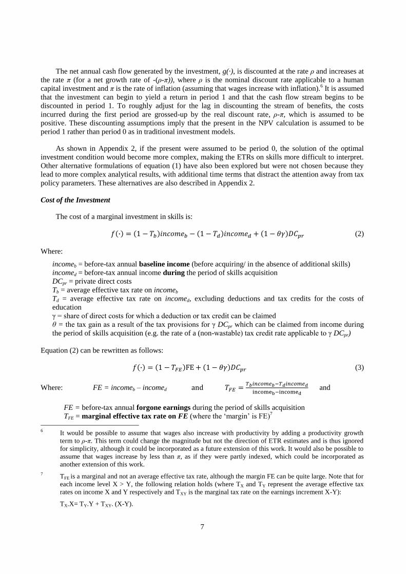
The net annual cash flow generated by the investment, g(·), is discounted at the rate ρ and increases at

the rate π (for a net growth rate of -(ρ-π)), where ρ is the nominal discount rate applicable to a human

capital investment and π is the rate of inflation (assuming that wages increase with inflation).6 It is assumed

that the investment can begin to yield a return in period 1 and that the cash flow stream begins to be

discounted in period 1. To roughly adjust for the lag in discounting the stream of benefits, the costs

incurred during the first period are grossed-up by the real discount rate, ρ-π, which is assumed to be

positive. These discounting assumptions imply that the present in the NPV calculation is assumed to be

period 1 rather than period 0 as in traditional investment models.

As shown in Appendix 2, if the present were assumed to be period 0, the solution of the optimal

investment condition would become more complex, making the ETRs on skills more difficult to interpret.

Other alternative formulations of equation (1) have also been explored but were not chosen because they

lead to more complex analytical results, with additional time terms that distract the attention away from tax

policy parameters. These alternatives are also described in Appendix 2.

Cost of the Investment

The cost of a marginal investment in skills is:

(2)

Where:

incomeb = before-tax annual baseline income (before acquiring/ in the absence of additional skills)

incomed = before-tax annual income during the period of skills acquisition

DCpr = private direct costs

Tb = average effective tax rate on incomeb

Td = average effective tax rate on incomed, excluding deductions and tax credits for the costs of

education

γ = share of direct costs for which a deduction or tax credit can be claimed

θ = the tax gain as a result of the tax provisions for γ DCpr which can be claimed from income during

the period of skills acquisition (e.g. the rate of a (non-wastable) tax credit rate applicable to γ DCpr)

Equation (2) can be rewritten as follows:

(3)

Where: FE = incomeb – incomed

and

FE = before-tax annual forgone earnings during the period of skills acquisition

TFE = marginal effective tax rate on FE (where the „margin‟ is FE)7

6 It would be possible to assume that wages also increase with productivity by adding a productivity growth

term to ρ-π. This term could change the magnitude but not the direction of ETR estimates and is thus ignored

for simplicity, although it could be incorporated as a future extension of this work. It would also be possible to

assume that wages increase by less than π, as if they were partly indexed, which could be incorporated as

another extension of this work.

7 TFE is a marginal and not an average effective tax rate, although the margin FE can be quite large. Note that for

each income level X > Y, the following relation holds (where TX and TY represent the average effective tax

rates on income X and Y respectively and TXY is the marginal tax rate on the earnings increment X-Y):

TX.X= TY.Y + TXY. (X-Y).

8

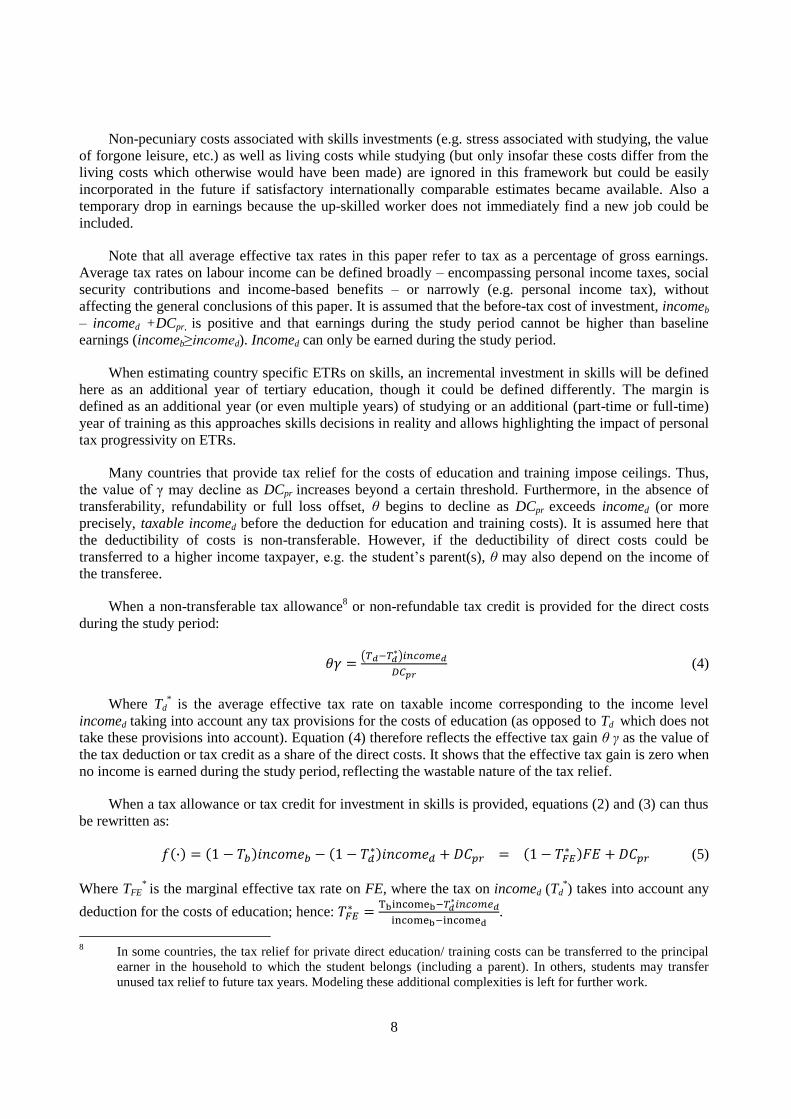
Non-pecuniary costs associated with skills investments (e.g. stress associated with studying, the value

of forgone leisure, etc.) as well as living costs while studying (but only insofar these costs differ from the

living costs which otherwise would have been made) are ignored in this framework but could be easily

incorporated in the future if satisfactory internationally comparable estimates became available. Also a

temporary drop in earnings because the up-skilled worker does not immediately find a new job could be

included.

Note that all average effective tax rates in this paper refer to tax as a percentage of gross earnings.

Average tax rates on labour income can be defined broadly – encompassing personal income taxes, social

security contributions and income-based benefits – or narrowly (e.g. personal income tax), without

affecting the general conclusions of this paper. It is assumed that the before-tax cost of investment, incomeb

– incomed +DCpr, is positive and that earnings during the study period cannot be higher than baseline

earnings (incomeb≥incomed). Incomed can only be earned during the study period.

When estimating country specific ETRs on skills, an incremental investment in skills will be defined

here as an additional year of tertiary education, though it could be defined differently. The margin is

defined as an additional year (or even multiple years) of studying or an additional (part-time or full-time)

year of training as this approaches skills decisions in reality and allows highlighting the impact of personal

tax progressivity on ETRs.

Many countries that provide tax relief for the costs of education and training impose ceilings. Thus,

the value of γ may decline as DCpr increases beyond a certain threshold. Furthermore, in the absence of

transferability, refundability or full loss offset, θ begins to decline as DCpr exceeds incomed (or more

precisely, taxable incomed before the deduction for education and training costs). It is assumed here that

the deductibility of costs is non-transferable. However, if the deductibility of direct costs could be

transferred to a higher income taxpayer, e.g. the student‟s parent(s), θ may also depend on the income of

the transferee.

When a non-transferable tax allowance8 or non-refundable tax credit is provided for the direct costs

during the study period:

(4)

Where Td* is the average effective tax rate on taxable income corresponding to the income level

incomed taking into account any tax provisions for the costs of education (as opposed to Td which does not

take these provisions into account). Equation (4) therefore reflects the effective tax gain θ γ as the value of

the tax deduction or tax credit as a share of the direct costs. It shows that the effective tax gain is zero when

no income is earned during the study period, reflecting the wastable nature of the tax relief.

When a tax allowance or tax credit for investment in skills is provided, equations (2) and (3) can thus

be rewritten as:

(5)

Where TFE* is the marginal effective tax rate on FE, where the tax on incomed (Td

*) takes into account any

deduction for the costs of education; hence:

.

8 In some countries, the tax relief for private direct education/ training costs can be transferred to the principal

earner in the household to which the student belongs (including a parent). In others, students may transfer

unused tax relief to future tax years. Modeling these additional complexities is left for further work.

9

Benefits of the Investment

During the expected holding period, over which the cost of investment is recovered, the annual after-

tax net cash flow (earnings increment) as a result of the skills investment is:

(6)

After the end of the expected holding period (i.e. if skills are used productively for more years than

initially anticipated),

(7)

Where:

incomea + λ(incomeb – incomed + DCpr) = before-tax annual income after completion of the investment

in skills

λ(incomeb – incomed + DCpr) = annual income necessary to recover the initial cost of the investment9

Ta = average effective tax rate on incomea + λ(incomeb – incomed + DCpr)

Equation (6) can be simplified as:

(8)

Where:

EI = incomea + λ (incomeb – incomed + DCpr) – incomeb

–

–

And:

EI = before-tax annual earnings increment during the holding period (i.e. the amount by which

income after making the investment exceeds baseline earnings)

TEI = marginal effective tax rate on EI (where the „margin‟ is the earnings increment)10

Non-pecuniary benefits associated with skills investments (e.g. the joy of learning, prestige, etc.) are

ignored in this framework, but could be easily incorporated in the future if satisfactory internationally

comparable estimates became available. Also the employment probability, which may increase if the skills

investment has been finalized successfully can be included as well as the probability that the skills

investment will not be finalized successfully and therefore no return will be realized despite of the costs of

the investment. Also, instead of assuming a fixed level of baseline earnings, the framework could be

adjusted such that data on actual earnings profiles can be included.

9

Unlike for other capital investments, this additional return is necessary to recover the initial costs of investing

in skills, given that human capital is embedded in individuals and cannot be sold.

10 In case only personal income taxes are considered and depending on the statutory PIT brackets, the TEI is a

weighted average of the marginal personal income tax rates over the EI interval (i.e. an „average‟ marginal

personal income tax rate).

10

EI, the before-tax earnings increment as a result of the investment, is the amount by which earnings

after making the investment exceed baseline earnings. The earnings premium could be thought of as the net

annual return (in NPV terms) to an incremental human capital investment. A positive earnings increment

indicates that the income earned as a result of a skills investment is more than enough to compensate for

the forgone baseline earnings (incomeb) and to recover the cost of investment over its expected holding

period [λ(incomeb – incomed + DCpr)]. The earnings increment that makes a person indifferent about

making a marginal (e.g. one-year) investment in tertiary education is defined as EIopt

. This amount is

endogenous and is derived below by solving equation (1) when V is set equal to zero.

Because human capital is an asset that is embedded in people and cannot be sold, the initial costs of

investment can only be recovered by earning an additional return. The annual return to recover the costs of

education is defined here as λ(incomeb – incomed + DCpr). This implies in equations (6) to (8) that the

original investment cost is assumed to be recovered gradually over 1/ periods regardless of the

probability of actually realizing a positive cash flow in period n. Although equations (1), (6) - (8) could be

formulated differently so that the original investment is recovered in exactly the period of time over which

a return is actually realized, it is likely that when a skills investment is being considered, prospective

students expect to recover the costs within a fixed number of years.11

For example, a student taking a loan

to finance his or/her studies generally has to repay it within a maximum number of years. The academic

literature on effective tax rates on skills disregards the term by assuming

that skills investments are held over an infinite holding period. By introducing this term, this framework

can be used to explore the impact of taxes on the incentive to invest in skills at different points in the life

cycle, including investments by older workers approaching retirement.

For simplicity, it is assumed that incomea (as well as incomeb and incomed) consists of labour income,

although it is possible for some of the returns to skills investments to be realized through self-employment

or other forms of income that entail capital income, and/or through higher pension income after retirement.

Also for simplicity, it is assumed that incomeb, Tb and λ remain constant every year over the life of the

investment.

Net Present Value of an Alternative Investment

An alternative marginal capital investment, whose original investment cost f(·) is fully recovered at

the time of the asset‟s disposition is defined by:

(9)

Where:

the nominal after-tax return on an alternative capital investment: (10)

r = the real interest rate, and π = the inflation rate

Tc = the average tax rate on capital income.

It is assumed that r > 0, π>0 and Tc<1, so ρ>0. Note that ρ is also the discount rate that applies to the

return on the skills investment (see equation (1)).

The first term of the summation in equation (9) is the NPV of the return on the investment, ρf(·), while

the second term is the NPV of the amount recovered at the time of the asset‟s sale, f(·). Thus, equation (9)

11

Moreover, re-formulating these equations would increase the analytical complexity of the tax wedge and ETR

estimates by introducing additional time terms. Instead, the framework in this paper focuses the attention on

tax parameters rather than on the impacts caused by the timing of the cash flow of benefits.

11

shows that the cost of an investment is not just the initial outlay, f(·), but also the expected return on that

outlay. Because the rate of return on the invested amount equals the rate at which it is discounted, the

integral in equation (9) simplifies to f(·).

Although all taxpayers in a country face the same real interest rate on savings deposits and the same

inflation rate, the return on an alternative investment may vary across age groups due to differences in

capital tax rates on different assets. For example, in the early years of an adult‟s working life, investments

may be made primarily in shares and bonds. Investments in residential housing are likely to come later in

life, followed by a focus on retirement savings. These different types of investments are likely to be taxed

at different rates in most countries, implying that the alternative investment return against which a human

capital investment is assessed can vary among taxpayers of different ages and across the life cycle. As a

future of extension of this work, the WP2‟s project on the taxation of household savings could be used to

provide estimates for Tc for different capital investments. The ETR on human capital could then be

estimated at different stages of the life cycle and in relation to specific alternative capital investments.

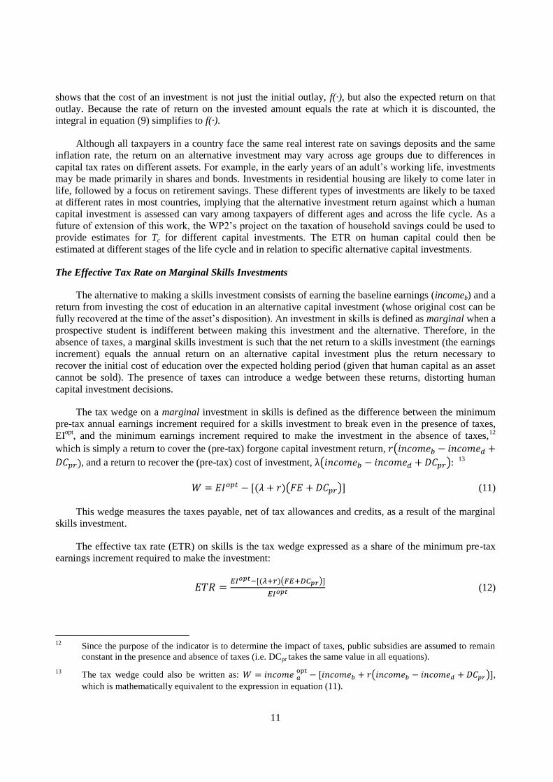
The Effective Tax Rate on Marginal Skills Investments

The alternative to making a skills investment consists of earning the baseline earnings (incomeb) and a

return from investing the cost of education in an alternative capital investment (whose original cost can be

fully recovered at the time of the asset‟s disposition). An investment in skills is defined as marginal when a

prospective student is indifferent between making this investment and the alternative. Therefore, in the

absence of taxes, a marginal skills investment is such that the net return to a skills investment (the earnings

increment) equals the annual return on an alternative capital investment plus the return necessary to

recover the initial cost of education over the expected holding period (given that human capital as an asset

cannot be sold). The presence of taxes can introduce a wedge between these returns, distorting human

capital investment decisions.

The tax wedge on a marginal investment in skills is defined as the difference between the minimum

pre-tax annual earnings increment required for a skills investment to break even in the presence of taxes,

EIopt

, and the minimum earnings increment required to make the investment in the absence of taxes,12

which is simply a return to cover the (pre-tax) forgone capital investment return,

and a return to recover the (pre-tax) cost of investment, 13

(11)

This wedge measures the taxes payable, net of tax allowances and credits, as a result of the marginal

skills investment.

The effective tax rate (ETR) on skills is the tax wedge expressed as a share of the minimum pre-tax

earnings increment required to make the investment:

(12)

12

Since the purpose of the indicator is to determine the impact of taxes, public subsidies are assumed to remain

constant in the presence and absence of taxes (i.e. DCpr takes the same value in all equations).

13 The tax wedge could also be written as:

,

which is mathematically equivalent to the expression in equation (11).

12

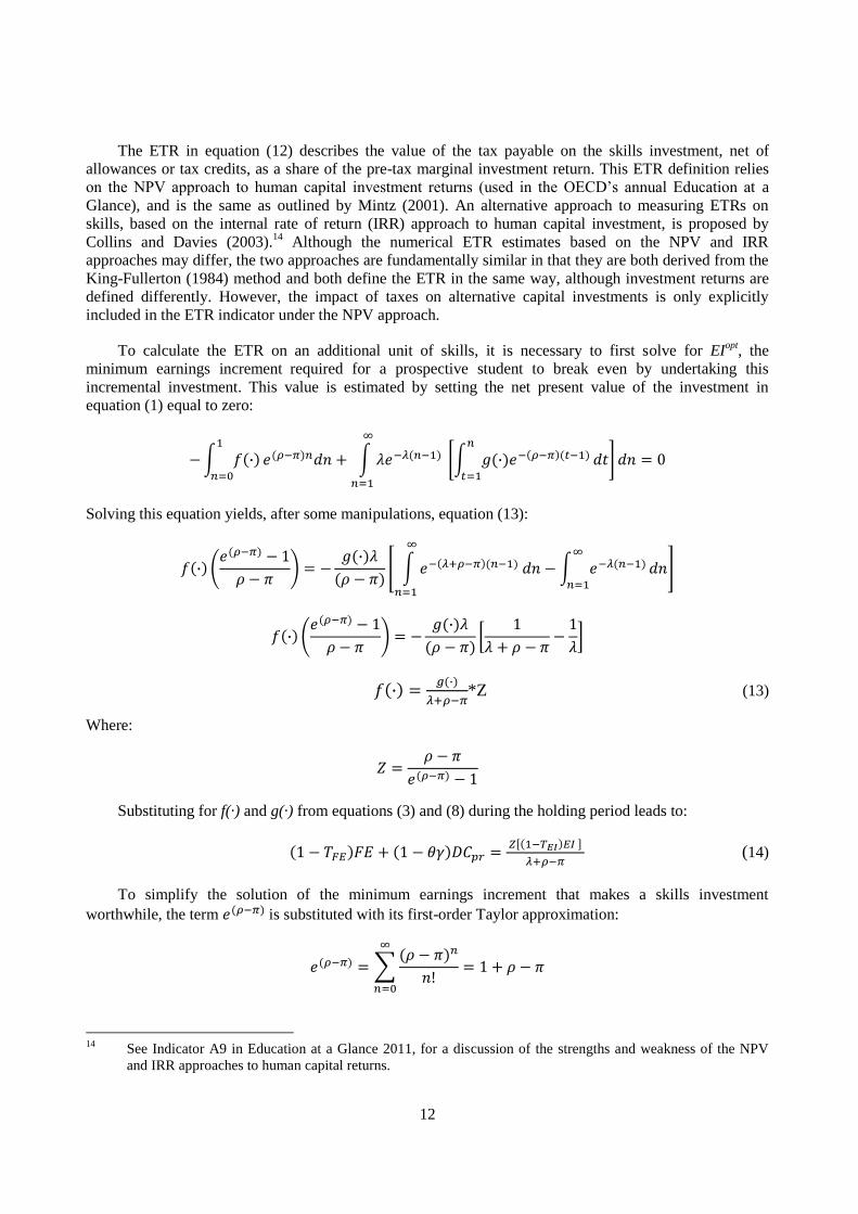
The ETR in equation (12) describes the value of the tax payable on the skills investment, net of

allowances or tax credits, as a share of the pre-tax marginal investment return. This ETR definition relies

on the NPV approach to human capital investment returns (used in the OECD‟s annual Education at a

Glance), and is the same as outlined by Mintz (2001). An alternative approach to measuring ETRs on

skills, based on the internal rate of return (IRR) approach to human capital investment, is proposed by

Collins and Davies (2003).14

Although the numerical ETR estimates based on the NPV and IRR

approaches may differ, the two approaches are fundamentally similar in that they are both derived from the

King-Fullerton (1984) method and both define the ETR in the same way, although investment returns are

defined differently. However, the impact of taxes on alternative capital investments is only explicitly

included in the ETR indicator under the NPV approach.

To calculate the ETR on an additional unit of skills, it is necessary to first solve for EIopt

, the

minimum earnings increment required for a prospective student to break even by undertaking this

incremental investment. This value is estimated by setting the net present value of the investment in

equation (1) equal to zero:

Solving this equation yields, after some manipulations, equation (13):

*Z (13)

Where:

Substituting for f(·) and g(·) from equations (3) and (8) during the holding period leads to:

(14)

To simplify the solution of the minimum earnings increment that makes a skills investment

worthwhile, the term is substituted with its first-order Taylor approximation:

14

See Indicator A9 in Education at a Glance 2011, for a discussion of the strengths and weakness of the NPV

and IRR approaches to human capital returns.

13

As a result, Z=1. Therefore, during the expected holding period, the minimum required pre-tax earnings

premium is:

(15)

Or, written alternatively:

(16)

Equation (15) shows that the income earned after making the skills investment and during the

expected holding period must be enough to cover (see appendix 5 for a graphical representation of EIopt

):

the forgone return on the after-tax cost of investment borne by the student:

An amount to gradually recover the after-tax cost of the investment over the holding period 1/λ:

The tax payable on EIopt

, by dividing the expression by (where TEI will depend on the

level of EI, and vice versa).

Equation (15) provides insights of the impacts of taxation even before estimating ETRs. For example,

it can be seen that when there is a flat tax on labour income (TFE=TEI=T) but the direct costs of education

are not fully deductible ( ), the minimum human capital return must be higher than otherwise to

make the investment worthwhile. The minimum return also has to be higher if the direct costs are fully

deductible during the period of studies but taxes are locally progressive (TEI>TFE).

Equation (15) can also be rewritten in terms of the minimum required incomea (

) which

needs to be earned:

i.e., the income earned after making the skills investment and during the expected holding period must

be enough to cover:

the forgone return on the after-tax cost of investment borne by the student:

the forgone wage income that would have been earned without making the investment:

when tax rates are not proportional or the direct costs are not deductible at the rate Ta, a premium

to compensate for the taxation of the portion of earnings that covers the cost of the investment:

14

, and

the tax payable on incomea, by dividing the expression by .

3. Interpretation of the ETR on skills

The ETR on skills, as defined in this paper, indicates the effective tax burden (net of tax credits and

allowances) on a marginal skills investment.

A tax system that is neutral with respect to marginal human capital investments results in an ETR of

0%. When the ETR is zero, the amount by which earnings increase (net of taxes) as a result of a skills

investment is just enough to recover the cost of investment (gradually) and to cover the forgone returns

from an alternative capital investment. This implies that prospective students are indifferent about

investing in skills at the margin. More generally, ETR estimates indicate whether the tax system creates

incentives or disincentives for taxpayers to make investments in human capital that would otherwise break

even. However, the decision to invest in skills is not purely driven by ETRs. For example, even if the tax

system is neutral, prospective students may choose not to invest in human capital if the net cash flow g(·)

required for the investment to break even is so high that it cannot be attained in the labour market after

completing an additional year of education. For example, this may the case when a taxpayer expects to

retire soon, since the (pre-tax) return needed to recover the original investment cost, i.e. λ(incomeb –

incomed + DCpr), may be too high to be covered with the expected annual income increase. This explains

why investments that yield identical income gains may be undertaken by younger but not by older adults,

since the additional lifetime income needed to recover the original investment can be spread over a longer

holding period (a lower λ) when the investment is made by a younger person. On the other hand, even if

the tax system is not neutral, a prospective student may choose to invest despite a positive ETR if the

investment yields (non-taxable) non-pecuniary benefits.

Behind the ETR on skills, which indicates the overall impact of the tax system on human capital

formation, there are two distinct factors at play. The ETR is partly driven by the impact of taxes on the

choice of whether to work and earn the baseline earnings or study and earn higher earnings in the future

(i.e. the work-study decision), and partly driven by the impact of taxes on the choice of whether to invest in

physical/financial capital and earn a capital income return or study and earn a labour income return (i.e. the

asset mix decision). By setting Tc to zero, it is possible to isolate the first component of the ETR, which is

the impact of labour income taxes alone. Thus, when Tc=0 and ETR=0, the personal tax system is

neutral with respect to human capital investments. More generally, when ETR=0 (regardless of Tc),

the overall income tax system is neutral both with respect to the asset mix and with respect to the

work-study decision. Note that in this paper, the personal tax system refers to taxes on labour income

(broadly or narrowly defined) and capital income taxes refer to taxes levied on capital (or rental) income

earned by individuals. The overall income tax system consists of personal taxes and capital income taxes.

The desirability of a neutral tax system depends partly on market failures or institutional disincentives

for skills formation that call for intervention and partly on the extent to which higher education and

training are publicly subsidized. Market failures and other disincentives may justify a negative ETR (i.e. a

favourable tax treatment of human capital), but generous public funding may warrant a positive ETR (i.e.

an unfavourable tax treatment of human capital). While a 0% ETR is not necessarily optimal, neutrality is a

benchmark that can be used to assess the impact of taxes on human capital formation decisions. The ETR

framework helps quantify this impact.

15

4. Analytical Results for Key Stylized Cases

The following case examples illustrate the various impacts of the tax system on the incentive to make

a marginal investment in skills. Most of them explore the neutrality of labour income taxes (i.e. the

neutrality with respect to the work-study decision) by assuming no capital income taxation (such that Tc =

0, so ρ=r+π). Case 2 does however look at the impact of capital income taxes on the asset mix. All the

examples relate to the minimum required before-tax income required for a marginal skills investment to

break even assuming that the investment yields a return (only) over the expected holding period (i.e. based

on equation (15) or (16)).

All case scenarios presented here assume that skills are supplied in the labour market once they are

acquired. For this purpose, labour supply is assumed to be inelastic, so that the indirect impact of taxes via

the incentive to work can be ignored.15

In this section, tax progressivity refers to average labour income tax rates that increase as earnings

rise, while flat tax rates refer to constant average labour income tax rates. Progressivity (or flatness) may

be global – referring to the entire income scale – or local – referring to increasing (or constant) average tax

rates within a particular range of income.

Case 1 – No Taxes on Labour or Capital Income: TFE = TEI = Tc = 0

Solving equations (15), (11) and (12) yields:

0%

As expected, in the absence of income taxes on labour or capital, the ETR on skills is zero and the tax

system is neutral, both with respect to the work-study decision and with respect to the asset mix.

Case 2 – No Tax on Labour Income, Tax on Capital Income: TFE = TEI = 0 and Tc > 0


The ETR on skills is negative because the minimum required EI for a marginal skills investment to break

even, net of the income required to pay for the cost of the investment (i.e. the λ term), is less than the pre-

tax return on an opportunity investment. The ETR is the negative value of the tax payable on the nominal

return to an alternative investment, expressed as a percentage of EIopt

. As indicated by the negative ETR,

when there are no taxes on labour income but there are taxes on capital income, the tax system

creates an incentive to pursue a marginal human capital investment. Human capital is favoured over

alternative capital investments, distorting the asset mix. This occurs because human capital returns are

not taxed but other investments are.

15

If labour supply is upward sloping, a flat tax system may discourage human capital formation for lower

income individuals (Jacobs, 2002).

16

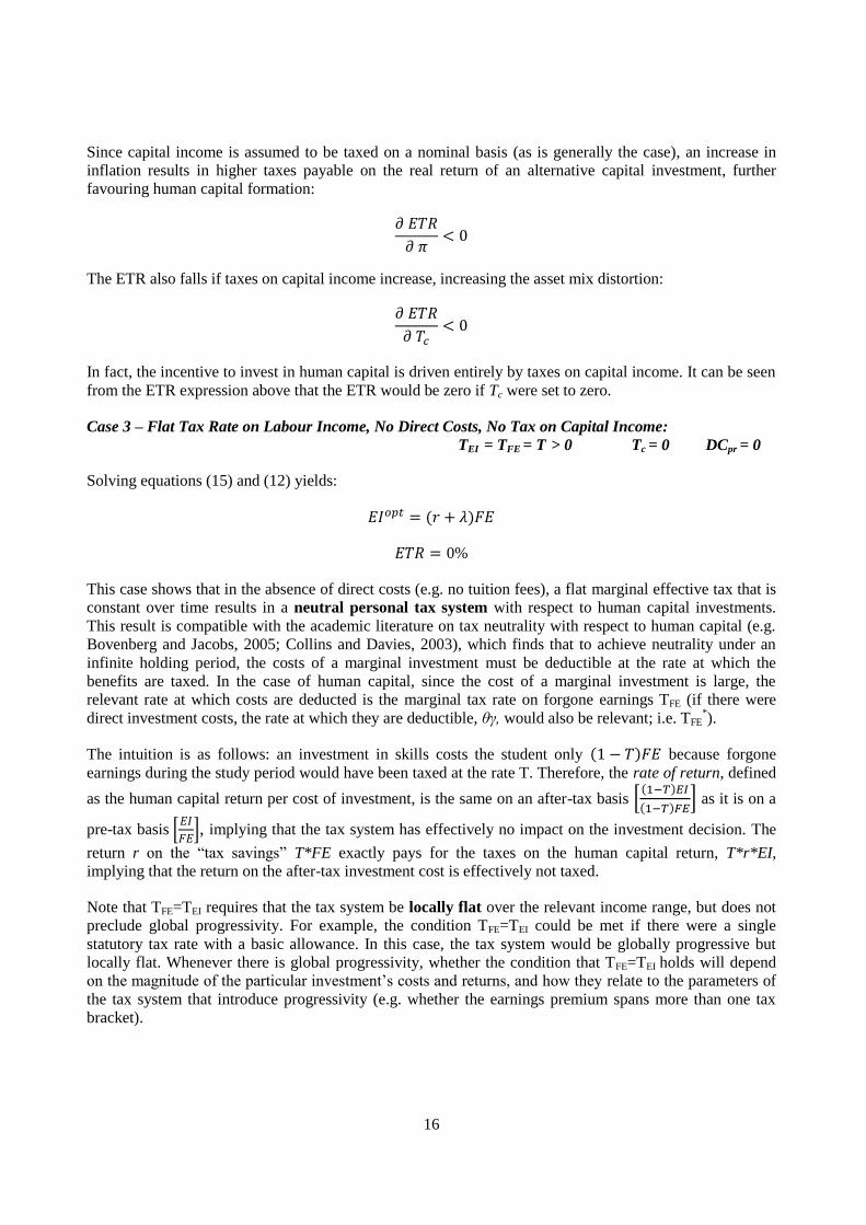
Since capital income is assumed to be taxed on a nominal basis (as is generally the case), an increase in

inflation results in higher taxes payable on the real return of an alternative capital investment, further

favouring human capital formation:

The ETR also falls if taxes on capital income increase, increasing the asset mix distortion:

In fact, the incentive to invest in human capital is driven entirely by taxes on capital income. It can be seen

from the ETR expression above that the ETR would be zero if Tc were set to zero.

Case 3 – Flat Tax Rate on Labour Income, No Direct Costs, No Tax on Capital Income:

TEI = TFE = T > 0 Tc = 0 DCpr = 0

Solving equations (15) and (12) yields:

0%

This case shows that in the absence of direct costs (e.g. no tuition fees), a flat marginal effective tax that is

constant over time results in a neutral personal tax system with respect to human capital investments.

This result is compatible with the academic literature on tax neutrality with respect to human capital (e.g.

Bovenberg and Jacobs, 2005; Collins and Davies, 2003), which finds that to achieve neutrality under an

infinite holding period, the costs of a marginal investment must be deductible at the rate at which the

benefits are taxed. In the case of human capital, since the cost of a marginal investment is large, the

relevant rate at which costs are deducted is the marginal tax rate on forgone earnings TFE (if there were

direct investment costs, the rate at which they are deductible, θγ, would also be relevant; i.e. TFE*).

The intuition is as follows: an investment in skills costs the student only because forgone

earnings during the study period would have been taxed at the rate T. Therefore, the rate of return, defined

as the human capital return per cost of investment, is the same on an after-tax basis

as it is on a

pre-tax basis

, implying that the tax system has effectively no impact on the investment decision. The

return r on the “tax savings” T*FE exactly pays for the taxes on the human capital return, T*r*EI,

implying that the return on the after-tax investment cost is effectively not taxed.

Note that TFE=TEI requires that the tax system be locally flat over the relevant income range, but does not

preclude global progressivity. For example, the condition TFE=TEI could be met if there were a single

statutory tax rate with a basic allowance. In this case, the tax system would be globally progressive but

locally flat. Whenever there is global progressivity, whether the condition that TFE=TEI holds will depend

on the magnitude of the particular investment‟s costs and returns, and how they relate to the parameters of

the tax system that introduce progressivity (e.g. whether the earnings premium spans more than one tax

bracket).

17

Case 4 – Flat Tax Rate on (Taxable) Labour Income, Full Deductibility of Direct Costs, No Tax on

Capital Income: 0 < TEI = TFE = T < 1 Tc = 0 DCpr > 0 γ = 1 θ = T


In this case, the direct costs are assumed to be fully deductible through a tax allowance (or a tax credit that

mimics a deduction), and the income against which the deduction is claimed (incomed) is high enough to

remain positive after netting out the deduction. Therefore, a constant flat tax rate with full deductibility

of the direct costs of skills formation results in a neutral personal tax system with respect to human

capital. This result is also compatible with the academic literature on tax neutrality with respect to human

capital (e.g. Bovenberg and Jacobs, 2005; Collins and Davies, 2003). The personal tax system is neutral

because the return to human capital is taxed at the same rate at which forgone earnings would be taxed and

the rate at which private costs are deductible (i.e. the rate at which education costs are implicitly

subsidized). Neutrality with respect to asset mix also is achieved because the return on an alternative

capital investment is taxed at a 0% rate. Note also that, even if the tax system is neutral in the presence of

direct costs, the minimum required earnings increment will exceed the required earnings increment in the

absence of direct costs (see case 3).

For the conclusion to hold more generally, when incomed <DCpr, it is also necessary for the deduction or

tax credit to be non-wastable, so that θγ can equal T independent of incomed. For example, if no income

is earned during the study period, θγ=T if a refundable tax credit is provided for the full amount of direct

costs and the credit is valued at the same rate as the average tax rate on labour income. In other words, T%

of the direct costs is reimbursed to students through the tax system. Alternatively, the ETR would be 0% if

the allowance could be carried over to future years (augmented by e(ρ-π)t

) and claimed against the income

earned after completing the investment. On a household basis, the ETR would be 0% if the allowance

could be transferred to another member of the household with sufficiently high income (e.g. the student‟s

parent), but only if the value of the transferred tax provision would not change.

Case 5 – Flat Tax Rate on (Taxable) Labour Income, Partial or Non-Deductibility of Direct Costs, No

Tax on Capital Income: 0 < TEI = TFE = T < 1 Tc = 0 DCpr > 0 0 ≤ θ γ < T


Therefore: if θ γ < T and if θ γ > T

18

This case shows that a constant flat tax rate with partial deductibility of the direct costs of skills

formation (θγ < T) results in a personal tax system that discourages marginal human capital

investments. The personal tax system is not neutral because it reduces the investments returns by more

than it reduces the direct costs, even though forgone earnings are reduced at the same rate as the

investment returns because of the flat tax rate.

The ETR expression above is a generalized version of that in case 4. If costs were fully deductible, so that

θγ=T, it can be seen that the ETR would be 0%. Note that unless the direct costs of education are fully

deductible, the ETR increases when the direct costs increase:

Thus, when the tax system does not provide full deductibility of the direct costs, policy changes that

increase the costs of education, such as increases in tuition fees or reductions in financial assistance to

students, are magnified by the tax system. The incentive to make a marginal human capital is reduced two-

fold, first because the direct costs increase and second because the ETR increases.

An important implication is that when the costs of education are not fully deductible, the ETR on

marginal skills investments can increase even in the absence of income tax policy changes. For

example, when there is partial deductibility of investment costs, the ETR will increase if tuition fees are

raised, or non-repayable financial assistance to students is reduced. Thus, post-secondary education policy

can affect the impact of the income tax system on human capital investments, and policy co-ordination

between finance and education ministries is advised. The ETR will also increase if sales taxes on

educational services increase (including a shift from zero-rating to VAT exemption), which increases the

price of the privately paid direct costs, highlighting the interaction between different taxes.

An increase in the rate at which the costs are deductible reduces the ETR, minimizing the disincentive to

pursue one more year of tertiary education:

Thus, the impact on ETRs of an increase in the private cost of education can be mitigated by

introducing or enhancing the deduction of costs for personal income tax purposes. To ensure the

allowance does not exclusively favour higher income taxpayers, low income taxpayers should be able to

benefit from the deduction, either through refundability or transferability over time or to other household

members.

Case 6 – Progressive Tax Rates on Labour Income, No Direct Costs, No Tax on Capital Income:

TEI > TFE ≥ 0 Tc = 0 DCpr = 0


19

The ETR is the difference between the marginal tax rate on the earnings increment and the marginal tax

rate on forgone earnings, per unit cost of investment (note that the cost of investment consists of forgone

earnings, which are reduced by TFE). Based on the internal-rate-of-return (IRR) approach and a discrete-

time methodology, Collins and Davies (2003) obtain the same ETR result when the holding period is

infinite and there are no direct costs.

As indicated by the positive ETR, when taxes are locally progressive over the relevant income range

(i.e. when TEI >TFE), the tax system discourages marginal human skills investments.

The gap between TEI and TFE can be interpreted as a rough indicator of local labour income tax

progressivity over the income range from incomeb to incomea and from incomed to incomea. Note that the

ETR increases as this gap widens:

Therefore, this case shows that the more progressive the income tax system, the larger the disincentive to

undertake a marginal skills investment.

The ETR expression above also indicates that if the tax system were locally regressive (TEI < TFE) – for

example, as a result of proportional personal income and social security contribution statutory rates

combined with ceilings on social security contributions – it would encourage marginal human capital

investments as the ETR would be negative. Because income-tested benefits may result in marginal

effective tax rates on labour income, which rise over certain income ranges and fall over others, they could

lead to either TEI ≥ TFE or TEI < TFE. Their impact on marginal investment incentives therefore depends on

the particular costs and benefits involved and the particular level of baseline earnings.

Even though the holding period is not an explicit term in the ETR expression above, it affects the ETR

through its impact on TEI If the tax system is locally progressive, an increase in λ will increase EIopt

, which

in case it has an (increasing) impact on TEI will increase the ETR.

This implies that when the tax system is progressive over the relevant income ranges, the negative impact

of a reduction in the expected duration of work after completing a human capital investment is magnified

by the tax system. The minimum earnings increment required to break even increases not only due to the

need to earn a higher annual return to recover the cost of the investment, but also because the tax rate on

the earnings premium increases.

Case 7 – Progressive Tax Rates on Labour Income, Direct Costs, No Tax on Capital Income:

TEI > TFE > 0 Tc = 0 DCpr > 0 0 ≤ θ γ ≤ TEI


If the direct costs are fully deductible at the rate TFE, the ETR is the same as in the absence of direct

costs (case 6):

. The introduction of direct costs has no impact on the ETR because

20

ultimately all costs are deductible at the same rate, whether they are direct or indirect. See also appendix 5

for a graphical representation of EIopt

.

Note that if the direct costs are fully deductible at the rate TEI, the ETR is lower than in the absence

of direct costs. Also, if direct costs are fully deductible, they will reduce taxable income that corresponds

to incomed, which may therefore result in a lower value of Td*, which in itself results in an increase in TFE

*,

which will reduce the ETR.

5. Numerical Estimates

This section presents some illustrative calculations which use certain OECD countries‟ systems as a

starting point, but which are not intended to represent ETRs for specific countries at this stage, so we will

refer to them as examples. The main aim of these calculations is to demonstrate how the presented

methodology can be applied in practice. As the ETR results are very tentative, they should be interpreted

with care.

The analysis focuses on the ETR on a year of tertiary education.16

The reference year for the

underlying data is 2011. As a follow-up project, ETRs will be calculated for all OECD countries using the

actual Taxing Wages country models; these results will be published in a follow-up paper.

Data and Assumptions

The following data sources have been used (and will be used as part of the follow-up project which

calculates ETRs for all OECD countries) to make assumptions about country-specific parameters:

Data on the direct costs of education in 2011 (variable DCpr), have been drawn from data published

in the OECD‟s Education at a Glance (2011 edition).

o Direct costs per student are defined as household expenditure on tertiary education per

tertiary student.17,18

o Rather than netting out subsidies given to students from the direct costs of education, they

are treated as income during the study period (i.e. they are assumed to reduce forgone

earnings rather than the direct costs of education). This distinction is necessary given the

generally different tax treatment of scholarship income and of the direct costs of education,

and is particularly useful because subsidies may exceed the direct costs of education.

Data on education subsidies received by tertiary students in 2011 have been drawn from data

published in the OECD‟s Education at a Glance (2011 edition). Subsidies per student are defined

as scholarships and grants19

to households per student.20

16

Z (see equation 13) has not been assumed equal to 1 for the purpose of the calculations.

17 Source: Tables B3.2b, B2.1, B1.1a, X2.2a in Education at a Glance (2011). 2007 data has been grossed-up by

the annual national increase in OECD Consumer Prices (MEI) dataset to reflect 2011 values.

18 Education at a Glance uses the same assumptions regarding direct costs of education gross of grants to

students for the purposes of estimating the net present value of a tertiary education degree.

19 The value of loan guarantees and loan subsidies (e.g. interest rate discounts) are ignored due to data

availability problems.

20 Source: Table B5.3, Table 2.1, Table B1.1a in Education at a Glance (2011). 2007 data has been grossed-up by

the annual national increase in OECD Consumer Prices (MEI) dataset to reflect 2011 values.

21

o In many countries, the education subsidies (e.g. scholarships and grants) are tax-exempt.

Although a separate subsidy variable could have been included in the model, the subsidies

are currently integrated in the before-tax annual income during the period of skills

acquisition (the incomed variable); the average tax rate on the corresponding income

(variable Td) has been adjusted in these countries where subsidies are not taxed or are not

taxed in the same way as labour income earned during the study period.

o Including the scholarships and grants as well as their tax treatment allows analysing the

impact of the possible double deduction that arises if scholarships and grants are not taxed

but direct costs are tax deductible.

Data about the anticipated retirement age (used to derive λ) has been drawn from data published in

the OECD‟s Pensions at a Glance (2011).21

The retirement age is assumed to be the expected

retirement age for men in year 2050.22

Information about statutory provisions that provide tax relief for the direct costs of tertiary

education (used to calculate θγ) has been drawn from country responses to the Taxation and Skills

questionnaire issued to country Delegates of Working Party No. 2 of the OECD‟s Committee of

Fiscal Affairs in 2011.

For simplicity, it has been assumed that baseline earnings (incomeb), and employment income

during the study period (incomed) are a fixed percentage of the national average wage of a full-

time worker in the private sector. While this improves the comparability of ETR estimates across

countries it may lead to less representative results on a country-by-country basis. Country-specific

education-earnings profiles could be used to check the sensitivity of ETR estimates to the baseline

and forgone earnings assumptions.23

The following assumptions have been made about country-independent parameters:

The nominal discount rate, ρ, is 5%;

The inflation rate, π, is 2%;

The tax rate on capital income, Tc, is 0%.

Assumptions about the discount and inflation rates may influence the magnitude of the ETR, but not

its direction (positive/negative). Assuming that the real (pre-tax) discount rate is 3% is consistent with

„Education at a Glance‟ indicators of the net present value of tertiary education.

On the other hand, assumptions about the tax rate on capital income (variable Tc) have more

significant implications. First, the value of Tc may in fact influence the direction of the ETR. Second, Tc is

likely to vary significantly not only across countries but also across asset types within countries. However,

Note that these subsidies include funds that may go indirectly to educational institutions, such as the subsidies

that are used to cover tuition fees, and funds that do not go, even indirectly, to educational institutions, such as

subsidies for students‟ living costs.

21 Source: Table 1.1 in Pensions at a Glance (2011).

22 In Education at a Glance, it is assumed that workers in all countries retire at age 64.

23 In Education at a Glance, it is assumed that forgone earnings during the study period are the national minimum

wage (or an equivalent). Baseline earnings after the study period are derived on ELS‟s age education-earnings

profiles.

22

given that the analysis of tax rates on personal savings is outside the scope of this paper and that no recent

OECD-wide estimates are available, capital income taxes have been ignored in the hypothetical ETR

calculations. Doing so is nevertheless informative by isolating the impact of taxes on labour income. That

is, the assumption that Tc=0 implies that the ETR estimates presented here focus purely on the impact of the

personal tax system on the work-study decision.24

These estimates could be elaborated in the future to

reflect both work-study and asset mix decisions by applying country-specific assumptions about Tc after

the OECD‟s project on the taxation of household savings is completed.25

To estimate the particular forms of tax relief claimed by tax filers, a number of additional assumptions

have been made (different/ additional assumptions can be made in the future ETR work); these

assumptions help determine whether the tax filer is eligible for education-related tax relief. For example,

tax relief may be age-specific, or contingent of being in full-time rather than part-time studies:

The tax filer is age 20.

The tax filer is enrolled for the first time in a tertiary education program (e.g. college/university)

as a full-time student.

As a simplifying assumption, education-related tax reliefs provided to parents (including

extended eligibility for child tax allowances contingent on their child‟s student status) or to

spouses of students are not being modelled. In particular, it is assumed that the student is not

claimed as anyone‟s dependant for tax purposes.

Other than tax reliefs for the costs of education, the tax filer claims standard tax reliefs except

when specifically ineligible as a result of the tax filer‟s age or student status. This applies to both

income earned during the study period, forgone earnings and income earned after completing the

investment. (I.e. the calculations do not take into account that labour income earned by a student

might be taxed differently than regular labour income).

Scholarships and grants to households assumed to be either tax-exempt or fully taxable, based on

the responses to the Tax and Skills questionnaire (Torres, 2012).

The costs of education are not financed with tax-favoured income other than the tax-exempt

grants described above, such as exempt scholarships received from academic institutions or

investment income in a tax-favoured education/ savings account.

In case the costs of education are financed with debt (student loans), it is assumed that the net

present value of the amortized loan equals the direct costs, i.e. it is assumed that the interest rate

on the loan equals the discount rate ρ.

As a future extension, additional forms of tax relief could be incorporated, for example, to explore the

impact of the difference possible sources of income used to finance education on the ETR on human

capital investments (e.g. tax-favoured education saving accounts). In the future when the methodology will

be applied to all OECD countries, the calculations would also have to take specific personal income tax

rules for student income into account.

24

As such, these estimates are comparable to those based on the IRR approach in Collins and Davies (2003).

25 The Tax Policy and Tax Statistics Division within the OECD Centre for Tax Policy and Administration is in

the process of calculating marginal effective tax rates on saving vehicles for OECD countries.

23

Methodological Application

The Tax and Skills (i.e. the extended Taxing Wages) models have been used to estimate average tax

rates Ta, Tb, Td, TEI, TFE and the effective deductibility rate, θγ (or Td*). With the Taxing Wages model, it is

possible to restrict or broaden the scope of personal taxes to personal income taxes (PIT) and/or social

security contributions (SSCs) and/or cash benefits.

The baseline case considered here consists of the following assumptions:

A) Baseline Case

The student is single and has no children.

The student‟s employment income during the study period is 25% of the average wage of a full-

time worker (e.g. from summer job earnings or part-time work during the academic year).

The student‟s tax-exempt grant income during the study period is country-specific.

Baseline earnings (in NPV terms) are 80% of the average wage.

The direct costs of a year of tertiary education are country-specific, and are meant to represent

the private direct costs of education paid by households (gross of subsidies).

Average tax rates reflect PIT, employee SSCs and benefits modelled in Taxing Wages.

To explore the impact of changes to particular parameters, the following scenarios are also explored:

B) PIT-only Case

Average tax rates reflect PIT only.

All other assumptions are like in Case A.

This case isolates the impact of personal income taxes.

C) No Student Earnings Case

The student earns no employment income while studying (i.e. incomed is 0).


Relative to Case A, this case reflects the impact of higher forgone earnings and of the lack of

eligibility for wastable tax relief for the direct costs of education, if any.

D) Single Parent Case

The student is a single parent with one child.


24

Relative to Case A, this case reflects the impact of child-related tax allowances, credits and benefits

on the average effective tax rate on forgone earnings and the average effective tax rate on the earnings

premium.

E) High Baseline Earnings Case

The baseline earnings are 120% of the average wage (i.e. 50% higher than in Case A).


Relative to Case A, this case reflects the impact of higher baseline earnings (and higher forgone

earnings), thereby reflecting the impact of local progressivity further up in the income scale.

Numerical results

The following tables indicate the ETR estimates under assumptions outlined above for a sample of

cases. These results are for illustrative purposes of the ETR methodology only, and no tax policy

conclusions should be drawn from the calculations. The ETR results should be compared with caution,

given that countries where ETRs are large might also provide more generous public funding for tertiary

education institutions. This impact does show up in the level of EIopt

which is increasing in the privately-

funded costs and therefore decreasing in the level of public funding. (The OECD‟s Education at a Glance

report provides more information on public expenditure indicators).26

The tables with numerical results, for the 5 cases that have been calculated, show (as a percentage of

the average wage) the level of the direct costs DC, the income that could be earned if the student would

work instead of study (incomeb), the minimum required earnings increment in order for the study to be

worthwhile to be undertaken (EIopt

), the tax wedge (TW) and the effective tax rate ETR.

An ETR of x% means that x% of the minimum required earnings increment is effectively paid in tax

as a result of the non-neutral tax treatment of the investment in skills. A negative ETR means that

investments in skills are effectively subsidized through the tax system.

The meaning of negative ETRs can best be explained with a simple example. Consider a lone parent

in country X that has a flat tax system, who works full-time but considers working part-time and studying

the rest of the time; assume also that the income earned when working part-time entitles the parent to a

high child benefit, but that this benefit is strongly reduced when income increases. The cost of working and

studying part-time, compared to working full-time (and earning baseline earnings), is therefore strongly

reduced by the tax system as the additional income that would be earned while working full-time is hit by

high marginal tax rates because of the benefit withdrawal (implying that the net-income between the two

different options would not differ too much). However, the return on skills formation (earnings increment)

will only be taxed at the flat tax rate. Because the tax system reduces the costs of studying (forgone net

earnings) more than that it reduces the after-tax increase in income, the lone parent faces a tax-induced

incentive to study, which would be reflected in a negative ETR on investment in skills.27

26

As a future extension, estimates of the net fiscal impact of government could be developed - see Appendix 3.

27 Negative ETRs may also arise if the forgone earnings would be taxed with employee SSCs but the earnings

increment would not (e.g. because of a SSC ceiling). The analysis, however, does not take into account that a

reduction in employee SSCs may lead to lower benefits in the future, implying that in this case the ETR results

should be interpreted with care.

25

In general, the calculated values of EIopt

are relatively low. Although the total costs of an additional

year of investment might be seen to be high, the impact on the minimum required yearly earnings

increment is relatively low as the costs have to be spread over a considerable period of time (on average

about 40 years until the student retires).

In general, we observe relatively low to very low ETRs, implying that these tax systems do not

strongly reduce incentives for skills formation (although, as noted before, these results are tentative and

should be interpreted with care). In the presence of positive taxes on capital income on alternative

investments, the ETRs on skills formation would further decrease. As expected, higher ETRs are observed

if the student does not earn income during his/ her study period and when the baseline earnings are 120%

instead of 80% of the AW. In both cases, the minimum required earnings increment EIopt

will be higher and

the effect of the progressivity of personal income tax systems will therefore be stronger. Low and even

negative effective tax rates can be observed in some cases for single parents, as a result of cash benefits

which are decreasing in income, thereby leading to higher marginal taxes on forgone earnings than on the

earnings increment.

In general, relatively low ETRs are a result of relatively constant (marginal) tax rates at higher income

levels (i.e. on earnings exceeding the baseline earnings) and relatively high marginal tax rates on forgone

earnings (for instance because of benefits and reductions in SSCs that are reduced with income). This is

exactly the observation that is made in the Special Feature of the 2012 edition of Taxing Wages (also

published as Paturot, Mellbye and Brys, 2013), which analyses tax progressivity. The analysis shows that

the average rate progressivity in the personal income tax system (including employee SSC) in most OECD

countries is implemented at the bottom of the income distribution and less at the higher end and that SSCs

have a flattening effect on progressivity. The results show large increases in average effective tax rates at

low income levels when income increases (i.e. high progressivity at the bottom), implying high marginal

effective tax rates on forgone earnings when investing in skills. Moreover, progressivity at higher income

levels is modest (on average across the OECD, although considerable differences across countries can be

observed), resulting in relatively constant marginal – although possibly at very high rates – effective tax

rates on the required earnings increment in order for the investment in skills to be worthwhile. The overall

impact is therefore relatively low disincentives for skills formation.

Some of the numerical results seem strongly influenced by the assumption that the student earns 25%

of the average wage, leading to high marginal tax rates on forgone earnings. As a result, the reduction in

the average effective tax rate as a result of cash benefits and/ or targeted income tax or SSC provisions

targeted at lower earnings affects the ETR less than the withdrawal of these provisions, which strongly

increases the marginal effective tax rates. In case student earnings are set to zero (case C), both of these

effects receive equal weight (as TFE will equal the average effective tax rate on incomeb instead of the

marginal effective tax rate on the difference between incomeb and incomed), resulting in a lower tax on

forgone earnings (TFE), thereby increasing the disincentives to skills formation.

The design of benefits and tax provisions that are withdrawn at higher earnings has therefore a strong

impact on incentives for marginal investments in skills; this is especially so if the forgone earnings lie in

the income zone where benefits and other tax provisions are tapered out. This leads to interesting policy

conclusions. For instance, if part-time workers which follow training during the rest of the available time

would receive more generous benefits than in the absence of training, these workers would face an

increased tax on forgone earnings and therefore a lower ETR on skills (and hence a stronger incentive to

follow training).

The results in the tables below are presented as a percentage of the particular country‟s yearly average

wage, except for the ETR in the last column.

26

Numerical results for example A

Case Scenario DC Income b EIopt

Tax Wedge ETR

(TW/EIopt

)

A – base case 1.8% 80% 2.8% -0.1% -3.8%

B – PIT only 1.8% 80% 3.2% 0.3% 8.9%

C – no student earnings 1.8% 80% 5.8% 1.5% 25.6%

D – single parent one child 1.8% 80% 2.8% -0.1% -3.1%

E – higher baseline earnings (120% of AW) 1.8% 120% 5.5% 0.4% 6.9%

Numerical results for example B


Tax Wedge ETR

(TW/EIopt

)

A – base case 3.8% 80% 3.2% 0.2% 7.2%

B – PIT only 3.8% 80% 3.1% 0.2% 6.0%


D – single parent one child 3.8% 80% 3.3% 0.4% 11.1%

E – higher baseline earnings (120% of AW) 3.8% 120% 5.3% 0.3% 4.9%

Numerical results for example C


Tax Wedge ETR

(TW/EIopt

)

A – base case 5.9% 80% 3.1% 0.2% 5.3%

B – PIT only 5.9% 80% 3.1% 0.1% 4.6%



E – higher baseline earnings (120%AW) 5.9% 120% 6.2% 1.1% 17.7%

Numerical results for example D


Tax Wedge ETR

(TW/EIopt

)

A – base case 11.3% 80% 3.9% 0.4% 9.8%

B – PIT only 11.3% 80% 3.8% 0.3% 7.9%




Numerical results for example E


Tax Wedge ETR

(TW/EIopt

)

A – base case 10.2% 80% 3.4% 0.2% 5.8%

B – PIT only 10.2% 80% 3.4% 0.2% 5.8%


D – single parent one child 10.2% 80% 2.5% -0.7% -25.9%


27

Numerical results for example F


Tax Wedge ETR

(TW/EIopt

)

A – base case 1.1% 80% 2.3% -0.1% -3.4%

B – PIT only 1.1% 80% 2.4% 0.0% -0.7%


D – single parent one child 1.1% 80% 2.3% 0.0% -1.9%


Numerical results for example G


Tax Wedge ETR

(TW/EIopt

)

A – base case 27.5% 80% 4.6% 0.5% 11.5%

B – PIT only 27.5% 80% 4.5% 0.4% 9.1%




6. Concluding observations

This paper has developed an ETR framework that can be applied to skills investments of different

characteristics (magnitude of forgone earnings, level of income during the study period, number of years

during which the skills will be used in the labour force, etc.) and used to make cross-country comparisons

of the impact of taxes on skills formation incentives. The framework can be used to estimate the impact of

targeted tax measures related to education and training, and thus contribute to an evaluation of such tax

expenditures. In principle, it could also be used to analyse other policies that affect the financing of skills

investments and how they interact with the tax regime to influence the financial incentive to up-skill.

This paper has examined the impact of the tax system on the incentive to invest in human capital by

applying the ETR framework in various scenarios, which demonstrate the economic intuition behind the

methodology. This framework is also used to determine the minimum return necessary for a human capital

investment to be worthwhile, to derive the analytical conditions necessary for tax neutrality (i.e. ETR=0)

with respect to marginal human capital investments and to explore possible sources of non-neutrality. As

such, this paper complements the analysis in “Taxes and Investment in Skills”, OECD Taxation Working

Paper No. 13.

A number of results from the ETR analysis are worth noting, including:

When the tax system is not neutral with respect to human capital, the ETR on marginal skills

investments can increase even in the absence of changes in income tax policy. For example, this

occurs when the tuition fees increase or when sales taxes on education services increase and the

costs of education are not fully tax-deductible.

Conversely, the impact of an increase in the private cost of education on ETRs can be mitigated

by introducing or enhancing the deductibility of education costs for personal income tax

purposes. Thus, tax policy should be co-ordinated with tuition fee policy to achieve the desired

28

impact of a tuition fee increase on the fiscal incentive to build human capital. Sales tax and

income tax policy should be similarly co-ordinated.

When the tax system is not neutral with respect to human capital, the ETR may increase as the

expected holding period decreases, depending on whether taxes are locally progressive over the

range that covers the earnings increment. Therefore, the tax disincentive to invest in human

capital may increase with age, reinforcing other disincentives to engage in adult training (e.g.

wage increases that are tied to seniority irrespective of skills levels, mandatory retirement, etc.)

as workers grow older.

When there is capital income taxation, the extent to which the tax system influences decisions to

invest in human capital depends on the capital income tax rate applicable to the alternative

investment. Therefore, the ETR may vary across the lifecycle as the tax rate on capital

investments pursued at a younger age (e.g. shares and bonds) may differ from the tax rate on

investments pursued later (e.g. residential housing).

The ETR on skills framework has been used to derive estimates of the ETR on a year of tertiary

education using the OECD Taxing Wages framework. The calculations are for illustrative purposes of the

ETR methodology only, and use examples that are generally based on the systems of certain OECD

countries but which are not meant to represent these countries specifically. The preliminary analysis has

found low values for the minimum required earnings increment and ETRs on skills formation. This seems

to imply that, on average across different types of degrees within each country, studying an additional year

for a student who will afterwards enter the labour market for at least 40 years is a profitable investment

opportunity. This might imply that there is room in some countries to increase private funding of direct

education costs. The numerical analysis has also pointed at the impact of the withdrawal of benefits and

other tax provisions targeted at lower-income workers. Benefit withdrawal may lead to high marginal

effective tax rates on forgone earnings, thereby reducing the disincentive to study and upgrade skills.

The ETR methodology presented in this paper aims to provide a general indication of the impact of

taxation on the incentive to pursue marginal investments. However, the complexity of skills investment

decisions could be built into the methodology, which could be further developed in a number of ways:

1. Not all students that start a year of education complete their studies successfully or within the

foreseen time span. A provision for this uncertainty could be incorporated into the model.

2. Additional skills increase the probability of being employed during the worker‟s career, even

though workers that have followed an additional qualification may not necessarily directly

find a new job or a job that matches the new level of skills. There might be search costs as

well. Therefore, the employment probability with and without additional skills (as well as

search costs), could be included in the ETR framework.

3. Skills may also depreciate over time, although this not necessarily is reflected into lower

labour earnings over time.

4. Additional pension income possibly arising from increased social security contributions as a

result of higher labour earnings are currently ignored, but they could be incorporated in the

framework.

5. Given that the decision to acquire additional skills is likely to involve factors beyond financial

incentives, the non-pecuniary costs and benefits associated with skills investments (e.g. stress

and pleasure associated with studying, the value of forgone leisure, prestige, etc.), as well as

29

other indirect costs of education (e.g. costs of living, insofar as these costs differ from those

which would otherwise be incurred), could be incorporated in the future if satisfactory

internationally comparable estimates became available. (Such an extension would result in a

framework which goes beyond an effective tax rate framework).

6. It has been assumed that the private costs of a skills investment are financed by the individual

who acquires the skills. This assumption could be relaxed to incorporate tax provisions

available to family members or spouses who support students or trainees during the period of

skills acquisitions. For example, parents may benefit from the tax deductibility of tuition

costs, or continue to receive child benefits when their adult children are in university, and

spouses may be able to transfer training-related tax reliefs between each other.

7. Students or workers could also finance their training through debt, which could also be

incorporated into the methodology to assess whether particular sources of finance,

particularly when they receive a different tax treatment, alter the minimum required earnings

increment and the effective tax rate on skills investments.

In addition, the current methodology could be used to evaluate whether it pays to study or up-skill

depending on the choice of occupation, age or other characteristics by comparing the calculated minimum

required earnings increment with actual earnings profiles. It could also be applied to calculate the

minimum number of years that a worker would need to use his/ her newly acquired skills for a training

investment to be worthwhile. The methodology could also be extended to evaluate whether government

earns back the publicly-funded marginal investment in skills.

As a next step, the ETR methodology presented in this paper will be applied to all OECD countries

and the results for each country will be discussed and validated with representatives from the respective

ministries of finance/treasuries before publication. Further analysis could also focus on the impact on the

required earnings increment as well as the ETR when the extent of public funding for higher education is

reduced and the amount of private funding by students is increased. In addition to focusing on a year of

tertiary education, the methodology will also be applied to other types of skills investment decisions, such

as the decision to pursue a Masters‟ degree (e.g. MBA) by a worker in his/her late 20s and the decision to

follow specialized training by a mid-career individual.

30

REFERENCES

Brys, B. (2005), Tax Arbitrage in the Netherlands, Evaluation of the Capital Income Tax Reform of

January 1, 2001, Tinbergen Institute Research Series, No. 344.

Bovenberg, A.L. and B. Jacobs (2005), “Redistribution and Education Subsidies are Siamese Twins,”

Journal of Public Economics, Vol. 89, pp. 2005-2035.

Collins, K.A. and J.B. Davies (2003), “Measuring Effective Tax Rates on Human Capital: Methodology

and an Application to Canada,” CESifo Working Papers, No. 965.

Heckman, J. (1976), “A Life-Cycle Model of Earnings, Learning and Consumption,” Journal of Political

Economy, Vol. 84, No. 4, pp. S11-S44.

Jacobs, B. (2002), “Chapter 2: Optimal Income Taxation with Endogenous Human Capital,” in Public

Finance and Human Capital, Thela Thesis, Amsterdam.

King, M.A. and D. Fullerton (1984), The Taxation of Income From Capital: A Comparative Study of the

United States, the United Kingdom, Sweden and Germany, University of Chicago Press.

Mintz, J. (2001), Most Favored Nation: Building a Framework for Smart Economic Policy, C.D. Howe

Institute, Toronto.

Nielsen, S.B. and P.B. Sorensen (1997), “On the Optimality of the Nordic System of Dual Income

Taxation,” Journal of Public Economics, Vol. 63, pp. 311-329.

OECD (1994), Taxation and Household Savings, OECD Publishing.

OECD (2011), Education at a Glance 2011: OECD Indicators, OECD Publishing.

OECD (2012), Taxing Wages 2010-2011, OECD Publishing.

Paturot, D., K. Mellbye and B. Brys (2013), “Average personal income tax rate and tax wedge progression

in OECD countries,” OECD Taxation Working Paper Series, No. 15.

Torres, C. (2012), “Taxes and Investment in Skills,” OECD Taxation Working Paper Series, No. 13.

31

Appendix 1

PROBABILITY DENSITY FUNCTION OF THE EXPONENTIAL DISTRIBUTION

The term is the probability density function of the exponential distribution, with location

parameter η and scale parameter λ. Its value indicates the probability that an investment will realize a

return (or cash flow) until time period n, after which no further return is earned. The inverse of the scale

parameter, 1/λ, is the expected holding period of the investment (e.g. the length of time during which skills

are used in the labour force). As the expected holding period increases (e.g. if the retirement age is raised)

the probability distribution is stretched out to the right; as it decreases it is compressed towards the origin

(i.e. the location parameter; see Figure A.1). The location parameter η shifts the beginning of the

probability distribution. In equation (1), it is assumed that the return to human capital can begin to be

realized in period 1, so that η=1.

Figure 1. Figure A.1: Effect of changes in λ, where the location parameter is 0

Source: Dr. Hanan M. Aly

The integral of the exponential density function from η to infinity,

implies that the

probability that the investment will yield a return in period n is 1 in period η and decreases exponentially as

n increases, reaching 0 as n→∞.

32

Appendix 2

ALTERNATIVE FORMULATIONS OF THE NET PRESENT VALUE OF A MARGINAL

SKILLS INVESTMENT


Equation (1) can be rewritten more generally as:

(1.1)

Where

The investment takes place between period 0 and period ψ

The expected holding period of the investment is 1/λ

The probability that the investment realizes a return becomes positive in period η

The net cash flow of benefits begins to be discounted in period φ

ρ is the nominal discount rate applicable to a human capital investment and π is the rate of

inflation

Because human capital is embodied in people and cannot be sold, the gains from “disposing the

asset” at the time of retirement are 0* e - ρ-π(n-η)

In equation (1), it is assumed that ψ= η= φ=1. If instead the cash flow of benefits began to be discounted

from period 0 (φ=0), as in a traditional NPV framework, equation 1.1 would be transformed into:

(1.2)

A marginal skills investment is defined by V = 0, so

This expression is more complex than equation 9(a) due to the presence of a time term. Although this

expression can be simplified by replacing e ρ-π

with its first-order Taylor approximation, the result remains

more complex than equation 9(a):

Therefore, by assuming that the cash flow begins to be discounted in period 1, equation (1) simplifies the

calculation of incomea*, the tax wedge and the ETR on skills. Replacing equation (1) with equation (1.2)

would not affect the sign of the ETR estimates in Section 3, although their magnitude would change if the

holding period is assumed to be finite.

Rather than assuming that the probability of realizing a return on a human capital investment follows the

exponential probability distribution, it could be assumed that a return is realized with certainty between

33

period 1 and period N. Assuming that the return begins to be discounted in period 0, the NPV of a skills

investment would then be described by:

(1.3)

Setting V = 0 results in:

While it is possible to find the value of incomea* by expanding this expression, the time terms involved in

this equation would greatly increase the complexity of the tax wedge and ETR estimates. Equation (1) has

been favoured over equation (1.3) to focus the attention on tax parameters rather than on the impacts

caused by the timing of the cash flow.

Finally, it could be assumed that the original investment cost is recovered over the precise holding period

N, rather than the expected holding period, 1/ λ. Assuming that the return begins to be discounted in period

0, the NPV of a skills investment would then be defined by:

(1.4)

Where:

Ta = average effective tax rate on

Setting V=0 to describe a marginal skills investment results in:

Where

Given the complexity of this expression, the analytical estimates of incomea*, the tax wedge and the ETR

on skills would be highly complex. Equation(1) is preferred over equation (1.3) in the proposed ETR

framework also because it may be unrealistic to assume that prospective students know with certainty the

number of years over which they will use the skills acquired from one year of education.

34

Appendix 3

THE NET FISCAL INCENTIVE FOR MARGINAL SKILLS INVESTMENT


As such, the ETR is not an appropriate indicator of the net impact of fiscal (tax and expenditure) policies

on skills formation. It is possible for generous public funding to more than offset the impact of tax

disincentives on marginal skills formation. As such, comparisons of ETRs on skills across countries may

be somewhat misleading, given that countries where ETRs are larger might also provide more generous

public subsidies for education. This issue is common to the comparison of any tax burden indicator across

countries, since they do not provide information about how tax revenues are used to provide benefits to

taxpayers.

To estimate the net fiscal impact of tax and education spending policies on the incentive to acquire

additional skills, the following indicators are proposed:

Net Fiscal Wedge:

Where EIopt

is the minimum earnings increment necessary for the investment to break even in the presence

of taxes and subsidies (as derived in equation 10), FENG is the value of forgone earnings assuming the

student receives no education-related grants or scholarships from the government, and DCtotal are the direct

costs of tertiary education in the absence of public funding for education (i.e. as estimated in scenario H of

the country ETR estimates).

The net fiscal wedge indicates the gap between the minimum necessary return in the presence of taxes and

subsidies, and the minimum necessary return in the absence of fiscal policy.

In the case of publicly-funded tertiary education, DCpr< DCtotal and FENG ≤ FE. This implies that, as long

as there is public funding for education, the net fiscal wedge will be smaller than the tax wedge, and could

possibly be negative even when the tax wedge is positive.

The net fiscal incentive could be defined as the net fiscal wedge expressed as a share of the return to a

marginal skills investment, for comparability purposes with the ETR:

35

Appendix 4

EXAMPLE-SPECIFIC CALCULATION PARAMETERS

It has also been assumed that the student is 20-years old, is single and has no children. The real interest rate

is 3% while the inflation rate is 2%. Taxes on capital income have been put to 0.

Example-specific parameters and variables (as a percentage of the country’s Average Wage)

Example A

Example B

Example C

Example D

SG (scholarships and grants) 4.3% 1.6% 4.8% 0.3%

Taxable SG income 0.0% 0.0% 0.0% 0.0%

DC (direct costs) 1.8% 3.8% 5.9% 11.3%

DC in the absence of government

spending 30.9% 36.2% 25.1% 16.2%

Non-refundable tax credit for DC none none 0 none

Refundable tax credit for DC (single) none 1.4% none none

Tax allowance for DC none none none none

Rho 0.05 0.05 0.05 0.05

Retirement age in year 2050 60 67 65 65

Years to retirement 39 46 44 44

Lambda 0.0256 0.0217 0.0227 0.0227

Example E

Example F

Example G

SG (scholarships and grants) 4.4% 10.1% 4.8%

Taxable SG income 0.0% 0.0% 0.0%

DC (direct costs) 10.2% 1.1% 27.5%

DC in the absence of government

spending 34.5% 35.9% 52.4%

Non-refundable tax credit for DC none none 0.5%

Refundable tax credit for DC (single) none none 0

Tax allowance for DC none none 0

Rho 0.05 0.05 0.05

Retirement age in year 2050 65 67 65

Years to retirement 44 46 44

Lambda 0.0227 0.0217 0.0227

Note that the amounts of refundable and non-refundable credits are calculated endogenously within the

extended Taxing Wages models.

36

Appendix 5

GRAPHICAL REPRESENTATION OF EIOPT

IN THE ABSENCE OF CAPITAL INCOME TAXES (TC = 0)

A graphically representation of EIopt

in equation (15) is presented in the following figure, where the dotted

line is the “non-studying incomeb” and the solid line shows the income that will be earned over time during

the study period and after having studied until the worker reaches the retirement age. It is assumed that Tc

equals 0; i.e. there are no taxes on capital income and, as a result , as in case 7.

Where the tax wedge „W‟ equals:

inc b - inc d

DC pr

λ(inc b - inc d + DC pr)

r (inc b - inc d + DC pr)

Tax Wedge 'W'

Retirement

inc a opt

inc d

EI opt

0

2

4

6

8

10

12

14

16

0 1 1 2 2 3 3 4 4 5 5 6 6 7 7 8 8 9 9 10 10 11 11

Non-studying income Studying income

Time (t)

Income level

Time (t)

Income level

Time (t)

Income level

inc b

37

OECD TAXATION WORKING PAPERS

No. 1 Tax reform trends in OECD countries

Bert Brys, Stephen Matthews and Jeffrey Owens

No. 2 What is a competitive tax system?

Stephen Matthews

No. 3 Making fundamental tax reform happen

Bert Brys

No. 4 Trends in top incomes and income inequality and the implications for tax policy

Stephen Matthews

No. 5 The evaluation of the effectiveness of tax expenditures: a novel approach. An application to

the regional tax incentives for business investments in Italy

Antonella Caiumi

No. 6 Corporate taxation and SMEs: the Italian experience

Marco Manzo

No. 7 Consumption taxation as an additional burden on labour income

Fidel Picos-Sánchez

No. 8 Non-tax compulsory payments as an additional burden on labour income

Bert Brys

No. 9 Taxation and innovation

Pamela Palazzi

No. 10 Wage income tax reforms and changes in tax burdens: 2000-2009

Bert Brys

No. 11 Shifting from social security contributions to consumption taxes: the impact on low-income

earner work incentives

Alastair Thomas and Fidel Picos-Sánchez

No. 12 Trends in personal income tax and employee social security contribution schedules

Carolina Torres, Kirsti Mellbye and Bert Brys

No. 13 Taxation and investment in skills

Carolina Torres

No. 14 Modeling the tax burden on labour income in Brazil, China, India, Indonesia and South

Africa

Luca Gandullia, Nicola Iacobone, Alastair Thomas

38

No. 15 Average personal income tax rate and tax wedge progression in OECD countries

Dominique Paturot, Kirsti Mellbye and Bert Brys

No. 16 Effective personal tax rates on marginal skills investments in OECD countries: a new

methodology

Bert Brys and Carolina Torres

39

THE OECD TAXATION WORKING PAPERS SERIES ON LINE

The OECD Taxation Working Papers Series may be found at:

The OECD Centre for Tax Policy and Administration website:

http://www.oecd.org/ctp/tax-policy/taxpolicyworkingpapers.htm

The OECD‟s online iLibrary: http://www.oecd-ilibrary.org/

The Research Papers in Economics (RePEc) website: www.repec.org

For further information on the OECD Taxation Working Papers Series, please write to:

[email protected].

Thursday 1 August: LB!

http://www.oecd.org/ctp/tax-policy/taxpolicyworkingpapers.htm

http://www.oecd-ilibrary.org/

http://www.repec.org/


Date post:	15-Apr-2017
Category:	Documents
Upload:	bert-brys
View:	25 times
Download:	0 times

Effective personal tax rates on marginal skills investments in OECD countries_Brys_Torres

Documents