Effectiveness of a feedback management procedure based on

Effectiveness of a feedback management procedure basedon controlling the size of marine protected areas throughcatch per unit effort

Mikihiko Kai and Kunio Shirakihara

Kai, M., and Shirakihara, K. 2008. Effectiveness of a feedback management procedure based on controlling the size of marine protected areasthrough catch per unit effort. – ICES Journal of Marine Science, 65: 1216–1226.

The effectiveness of a feedback management procedure using marine protected areas (MPAs) was investigated. This procedure doesnot control fishing effort, but it does increase the size of the MPA when the catch per unit effort (cpue) is below a predeterminedtarget level and reduces the size when the cpue is above this level. Stability analyses of the approach, which consisted of a populationdynamics model and a model to control MPA size, suggest that this procedure can lead to recovery of a depleted population andsustain that population at a predetermined target level, even when there is hyperstability (a non-linear relationship between popu-lation size and cpue). An alternative procedure using fishing effort instead of MPA size may also function well, although both pro-cedures may need a long time for a depleted population to approach the target level. Performance of both procedures wasexamined using numerical simulations focused on system dynamics in the short term after management implementation. The pro-cedure using MPA size was more effective at preventing population collapse. Simulations suggest that if this procedure starts from adesirable level of initial MPA size, it has advantages over the alternative procedure through creating speedier population recovery anda higher level of short-term catch.

Keywords: catch per unit effort, feedback control, hyperstability, marine protected area, population collapse.

Received 12 September 2007; accepted 1 June 2008; advance access publication 27 June 2008.

M. Kai: National Research Institute of Far Seas Fisheries, 5-7-1, Orido, Shimizu, Shizuoka 424-8633, Japan. K. Shirakihara: Ocean Research Institute,University of Tokyo, Nakano-ku, Tokyo 164-8639, Japan. Correspondence to M. Kai: tel/fax: þ81 543 366035; e-mail: [email protected].

IntroductionAttention has recently focused on the use of marine protectedareas (MPAs) in protecting habitats and maintaining ecologicalfunctions. MPAs serve as a means of managing exploited popu-lations by imposing bans on fishing in defined areas. They arealso referred to as closed areas, no-take zones, or fisheriesmarine reserves, and have been implemented to help replenishtarget populations, enhance recruitment, or protect habitatsused by critical life-history stages (Jones, 2002). Although MPAshave sometimes been used to supplement management based oncatch quota or fishing effort limitation, they have advantagesover management strategies that require knowledge of populationparameters to determine suitable levels. For example, overestima-tion of a total allowable catch may exhaust certain populations(Karagiannakos, 1996). However, MPAs can maintain a constantnumber of individuals by sheltering sedentary populations(Hastings and Botsford, 1999) and can improve the status ofmobile populations (Guenette and Pitcher, 1999). MPAs reducevariability in catches in the face of stochastic events such as recruit-ment failures (Sladek-Nowlis and Roberts, 1999; Rodwell andRoberts, 2004). In this sense, MPAs can be robust to uncertaintyin populations and fisheries.

A feedback management procedure (FB) was proposed byTanaka (1980), by which catch is controlled to achieve a targetpopulation size. This process does not require population

dynamics models or their parameters and is robust to uncertain-ties in estimates of population size and fishery impacts. As anextension, Harada et al. (1992) proposed a FB based on controllingfishing effort (Effort-FB) instead of catch.

Kai and Shirakihara (2005) proposed a FB based on controllingthe size of an MPA (MPA-FB), increasing the size of the no-takearea when the population is below a predetermined target level,and reducing it when it is above that level. They predicted thatthe FB can sustain the population at the target level withoutdirectly controlling the catch quota or fishing effort if the targetlevel is set to equal or exceed the maximum sustainable yield(MSY) and if a drastic change in MPA size is avoided.

One difficulty in adopting the FB proposed by Kai andShirakihara (2005) is that the absolute population size, which isused in controlling MPA size, is not always known. If the catchper unit effort (cpue), which is available for many populations,can be used as an index of the population size, the FB will be effec-tive. However, the direct relationship between the cpue and thepopulation size cannot always be determined. The worst case formanagement is that the cpue remains high while the populationdeclines. Clark (1982) suggested a non-linear relationshipbetween them. This is also known as “hyperstability” (Hilbornand Walters, 1992), and evidence of this has been reported inseveral papers (e.g. Harley et al., 2001). Hyperstability mayreduce the effectiveness of the FB using cpue, because it may

# 2008 International Council for the Exploration of the Sea. Published by Oxford Journals. All rights reserved.For Permissions, please email: [email protected]

1216

Dow

nloaded from https://academ

ic.oup.com/icesjm

s/article/65/7/1216/645727 by guest on 04 January 2022

allow high-fishing pressure even when the population is depleted.However, the management effect is unlikely to be the samebetween the MPA-FB and the Effort-FB in that the former cansave individuals in MPAs.

We investigated the effectiveness of the MPA-FB using the cpueand compared it with the corresponding Effort-FB from three per-spectives: (i) whether the management procedures using the cpue(hereafter, MPA-FB and Effort-FB refer to the procedures usingthe cpue) successfully approach a predetermined populationtarget level; (ii) whether the procedures can prevent collapse ofdepleted populations with stochastic fluctuations; and (iii) whatadvantages and disadvantages each FB possesses.

Basic modelsTo examine the effectiveness of the MPA-FB, we use a discretedynamic model for an exploited population:

Ntþ1 � Nt ¼ GðNtÞ � Ct; ð1Þ

where N is the absolute population size, G a function of the popu-lation increase, C the catch, and t the year. The model used todescribe each FB is

Stþ1 � St ¼ �hUt

Utarget� 1

� �for MPA-FB; ð2Þ

Xtþ1 � Xt ¼ hUt

Utarget� 1

� �for Effort-FB; ð3Þ

where S is the MPA size, X the fishing effort, h a positive constant,U the cpue, and Utarget a target level cpue. Equation (2) shows anincrease in S when U is below Utarget, and a decrease in S when Uis higher than Utarget. A system for the MPA-FB is given by com-bining Equations (1) and (2), where C is a function of N andS. In this system, X is not controlled directly. To determinewhether population recovery can be attained only by controllingS, effort X is assumed to be constant. A system for the Effort-FBis given by combining Equations (1) and (3), where S is equal to0 and C is a function of N and X.

We assume that the following relationship between U and N(Clark, 1982) holds:

U / Na; ð4Þ

where a is constant. This power function can describe various situ-ations. When a = 1, U is proportional to N. When 0 , a , 1, thefunction reproduces the hyperstability on which we focus. Weassume that 0 , a � 0.99 describes not only the hyperstabilitybut also approximately the proportionality. Stability and dynamicsof the systems are examined under the constraint of Equation (4).

Equation (4) shows that U is uniquely determined from N, andmay not be applicable to the MPA-FB because the observed valueof U depends on areas in which MPAs are placed: U is high whenall MPAs are placed in areas of low density, and low when in areasof high density. Therefore, the MPA-FB that controls S with Urequires special attention to U. This is a disadvantage of theMPA-FB relative to the Effort-FB. To cope with this difficulty,we assume that MPAs are temporarily removed for a short timebefore the fishing season of each year. Fishers can then utilizethe whole fishing ground freely. They earn their money from

fishing but should report the fishing area, the catch, and theeffort. Using the catch and effort from this experimental fishing,U for the whole ground can be calculated, and areas of highdensities where MPAs can be placed are evaluated. We furtherassume that the experimental catch is small enough so thatEquation (1) holds.

Stability of the systemsTo determine whether the two systems can direct N to Ntarget

(a target level of N) obtained from Utarget and Equation (4), weexamined the local stability, that is, the dynamic properties inthe neighbourhood of the equilibrium point: (N*, S*) for theMPA-FB system, and (N*, X*) for the Effort-FB system. Thepoint is stable, if state variables (N and S for the MPA-FBsystem, N and X for the Effort-FB system) return to the pointwhen a small perturbation causes the variables to depart fromthis point. If the following conditions are fulfilled, the point islocally stable (Bulmer, 1994):

A ¼ a11a22 � a12a21 , 1 and

B ¼ ja11 þ a22j � ða11a22 � a12a21Þ , 1:

Here, the system we consider is generally described as y1,t+1 = f1(y1,t, y2,t) and y2,t+1 = f2 (y1,t, y2,t), and a is the partial derivative atthe equilibrium point aij =[@f/@yj]*. Thus, y1 = N and y2 = S forthe MPA-FB system, and y1 = N and y2 = X for the Effort-FBsystem.

We assume that the population growth function G(N) showsdG/dN = 0 only at NMSY (the population size yielding MSY),which is satisfied by the logistic model or more generalizedPella–Tomlinson-type production model (Pella and Tomlinson,1969): G(N) = rN 2 rNc/K, where r is the intrinsic growth rate,K the carrying capacity, and c the shape parameter. We treat thestability only when the target population level is set at NMSY. Weregard the catch C as having the following properties:

@C

@S, 0 for MPA-FB; ð5Þ

@C

@X. 0 for Effort-FB; ð6Þ

0 ,@C

@N

� ��, 1 for both FBs: ð7Þ

Equation (5) shows that an increase in S in a given year leads toa decrease in C within that year. Equation (6) shows that anincrease in X in a given year leads to an increase in C withinthat year. Equation (7) is derived as follows:

@C

@N

� ��¼

@ðENÞ

@N

� ��¼

@E

@N

� ��N� þ E ¼ E;

where E (0 , E , 1) is the rate of exploitation in a given year. Thepartial derivative [@E/@N]* is given under a constant level of S orX, so that the increase in N does not change E, i.e. [@E/@N]* = 0.

Controlling the size of MPAs through cpue 1217

Dow


ic.oup.com/icesjm


The MPA-FB system can be summarized using Equations (1),(2), and (4):

Stþ1 � St ¼ �hNa

t

Natarget

� 1

!: ð8Þ

At equilibrium (Nt+1 = Nt and St+1 = St),

GðN�Þ ¼ C� and N� ¼ Ntarget;

where C* is a function of N* and S*. If this system has multipleequilibrium points, N may change irreversibly (Shirakihara andTanaka, 1978). Here, we will prove that the number of points is1 at maximum.

Because N* is uniquely determined, C* is a function of S*.G(N*) = C* can be rewritten as follows, considering that its leftside is a constant when the function G is known:

C�ðS�Þ ¼ constant:

From Equation (5), the value of C corresponds to the value of S.Therefore, S* is also uniquely determined. The correspondingEffort-FB system can be summarized using Equation (1) and

Xtþ1 � Xt ¼ hNa

t

Natarget

� 1

!; ð9Þ

also has 1 or 0 equilibrium point. This is proved in a similar way,except that an increase in X in a given year leads to an increase in Cin that year.

We now examine the local stability of the MPA-FB system[Equations (1) and (8)]. Partial derivatives at an equilibrium point are

a11 ¼ �@C

@N

� ��þ1;a12 ¼ �

@C

@S

� ��;a21 ¼ �

ah

Ntarget;a22 ¼ 1:

Then,

A ¼ �@C

@N

� ��þ1�

@C

@S

� �ah

Ntarget

� �and

B ¼ 1þ@C

@S

� �ah

Ntarget

� �:

Because [@C/@S]* , 0 from Equation (5), B , 1 holds. Toshow that A , 1, we add a constraint; we set h at a sufficientlysmall value. In other words, we change S only slightly. As hbecomes smaller, A becomes smaller. When h = 0, A is equal to2[@C/@N]* + 1, which from Equation (7) is less than unity. Insummary, when Ntarget is set at NMSY and S is changed slightly,the equilibrium point is stable.

The local stability of the Effort-FB system [Equations (1) and(9)] can be examined in a similar way. Partial derivatives under

[dG/dN]* = 0 are

a11 ¼ �@C

@N

� ��þ1;a12 ¼ �

@C

@X

� ��; and

a21 ¼ah

Ntarget;a22 ¼ 1:

Then,

A ¼ �@C

@N

� ��þ1þ

@C

@X

� �ah

Ntarget

� �and

B ¼ 1�@C

@X

� �ah

Ntarget

� �:

With the aid of [@C/@X]* . 0 from Equation (6), it is proved thatthe equilibrium point is stable.

Note that our local stability analysis never guaranteesmanagement success when N is far from N*. It is difficult toprove the global stability of the systems analytically, but ournumerical analysis (see Appendix) suggests that the systems areglobally stable.

Specific modelsWe considered deterministic systems that are described by basicmodels. We proved that the systems are locally stable andsuggest that they are globally stable. Therefore, the basic modelsdo not account for population collapse. To examine the perform-ance of the FBs, such as robustness against collapse, we consideredstochastic population dynamics using the models specified below.First, the growth function G(N) was specified as a stochasticversion of the logistic model:

GðNÞ ¼ rN 1�N

K

� �1;

where 1 is the lognormal distribution with mean 1 and variance s2.We assume that the population will become extinct without failonce N � Nthreshold (the minimum level required for the populationto exist). Second, the catch C was specified:

Ct¼ Nbt �

StKb

T

� �1=b

� Nbt �ðStþX0ÞK

b

T

� �1=b

for MPA-FB; ð10Þ

and Ct¼Nt� Nbt �

XtKb

T

� �1=b

for Effort-FB; ð11Þ

where b = 1 2 a, T is the area that the population can inhabit, andX0 is a constant fishing effort evaluated by the area swept by thefishery. Equation (10), which has a complicated form, was usedbecause it can describe the hyperstability (Figure 1) and has sometheoretical basis in terms of the relationship between catch andMPA size (see Kai and Shirakihara, 2005, for its derivation).Equation (11) was derived from Equation (10) by making St = 0and replacing X0 with Xt. Third, the expected cpue, Uexpected,t,from experimental fishing in the MPA-FB was specified by assumingthat the experimental catch is equal to that calculated fromEquation (10) under St = 0 and Xt = X0, i.e. Uexpected,t = Ct/X0,where Ct = Nt 2 (Nt

b 2 X0Kb/T)1/b. Note that Equation (10) was

1218 M. Kai and K. Shirakihara

Dow


ic.oup.com/icesjm


derived under the situation in which fishers always exploit thehighest existing concentrations of fish (Kai and Shirakihara,2005). This situation is plausible when they freely access allfishing grounds. The expected cpue for Effort-FB is provided byEquation (11) and Xt. Finally, we considered a stochastic situationof Ut = Uexpected,t + Ft, where F is the normal distribution withmean 0 and constant variance, to investigate the effect of uncer-tainty in cpue.

In summary, each system is described as follows.

MPA-FB: Stþ1 � St ¼ �hUt

Utarget� 1

� �; ð12Þ

where Ut ¼ ½Nt � ðNbt � X0Kb=TÞ1=b

�=X0 þFt ,

Ntþ1 � Nt ¼ rNt 1�Nt

K

� �1t � Nb

t �StK

b

T

� �1=b

þ Nbt �ðSt þ X0ÞK

b

T

� �1=b

:

ð13Þ

Effort-FB: Xtþ1 � Xt ¼ hUt

Utarget� 1

� �; ð14Þ

where Ut ¼ ½Nt � ðNbt � XtK

b=TÞ1=b�=Xt þFt;

Ntþ1 � Nt ¼ rNt 1�Nt

K

� �1t � Nt þ Nb

t �XtK

b

T

� �1=b

: ð15Þ

Simulations using the specific modelsBecause the models above are specific examples of the basicmodels, the stability properties derived from the basic modelsare applicable to the specific models, although stochastic vari-ations in population size are introduced. Therefore, we canexpect the population to fluctuate randomly around the targetlevel when enough years have passed since implementation ofeach FB. Here, we focused on the dynamics of the systems in theshort term (5 or 10 years), specifically to assess whether successfulrecovery of the population and a sufficient level of catch can beachieved by implementing each FB. The performance of each FBwas examined using numerical simulations. To reduce thenumber of parameters, variables were transformed: nt = Nt/K, st

= St/T, xt = Xt/T, ct = Ct/K, ut = ct/xt + wt, where wt is the

normal distribution with mean 0 and variance j2. These allowedthe following equations to be derived:

MPA-FB : stþ1 � st ¼ �hut

utarget� 1

� �;

ntþ1 � nt ¼ rntð1� ntÞ1t � fðnbt � stÞ

1=b� ½nb

t � ðst þ x0Þ�1=bg:

Effort-FB : xtþ1 � xt ¼ hut

utarget� 1

� �;

ntþ1 � nt ¼ rntð1� ntÞ1t � ½nt � ðnb � xtÞ

1=b�:

We assumed that the population keeps an equilibrium statewithout random fluctuations when t = 0, i.e. n0 is a constant. Tocompare the performance of each FB, we gave a constraint thatn0 is the same in the two FBs. By putting nt+1 2 nt = 0 and 1t =1 in the last equation, the following relationship was obtained:

r ¼n0 � ðn

b0 � x0Þ

1=b

n0ð1� n0Þ:

Three parameters, r, b, and x0, could not be changed freely, and rwas determined uniquely from b and x0. To make r a real number,n0

b 2 x0 � 0 should be satisfied.In carrying out our simulations, values of the following nine

parameters were specified: n0 (transformed initial populationsize), h, s2 (constant variance of 1t), nthreshold (threshold level ofn), utarget (target level of u), s0, b, x0, and j2 (constant varianceof ft). For the first five parameters (n0 to utarget) that are expectedto have little effect on the performance ratio between the two FBs(explained below), their values were fixed: n0 = 0.1 (N0 = K/10,assuming that the population has been overfished before startingthe FBs), h = 0.005 (the annual increment of s or x is 0.0025when ut/utarget = 0.5), s2 = 0.3 (1 ranges from 0.321 to 2.39 witha probability of 0.95), nthreshold = 0.05 (Nthereshold = K/20), andutarget = uMSY (cpue giving nMSY = 0.5). We had concern aboutthe remaining three parameters, s0, x0, and b, where s0 and x0

are expected to affect the system dynamics in the short term andb describes the degree of non-linearity between cpue and thepopulation size. In the MPA-FB, s0 was arbitrarily given withinits possible range of 0 � s0 � 1, whereas in the Effort-FB, s0 wasfixed at 0. The parameters b and x0 were changed freely withintheir ranges in both FBs: 0 , b , 0.5 (proportionality or hyperst-ability was reproduced in this range) and 0 , x0 � 0.32 (this wasderived from the condition of n0

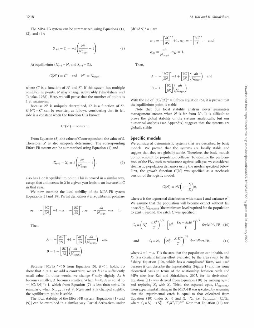
b 2 x0 � 0 and n0 = 0.1). Figure 2shows the interrelationship among the three parameters of r, b,and x0. The parameter r increased as x0 became higher as aresult of the constraint of keeping n0 = 0.1. Also, r increasedwith b except when x0 was high. The degree of the stochasticvariations ut was given by a CV (coefficient of variation) ofj/uexpected,0, whose possible range was set to be 0–200%.

A simulation trial was performed to reproduce annual changesin variables (n, s, and c for the MPA-FB, and n, x, and c for theEffort-FB) for at least 10 years under a set of parameter values.Such trials were repeated with different series of randomnumbers. Once n was below nthreshold in a given year, the populationwas regarded as having collapsed. However, the simulation was con-tinued, to trace the variables in subsequent years.

Figure 1. The relationship between population size and cpuederived from the specified models: U / N12b. When b = 0.49 andb = 0.01, the models can reproduce hyperstability andproportionality, respectively.


Dow


ic.oup.com/icesjm


To examine the effectiveness of the FBs, we used three perform-ance indicators:

(i) Mean population size. In each FB, the mean population sizeover the first or the second 5 years was calculated fromeach simulation trial. The mean and the variance weregiven from 100 trials. The performance ratio concerningthis quantity was defined as �nMPA�FB= �nEffort�FB, where

�nEffort�FB and �nEffort�FB are the means over 100 trials for theMPA-FB and Effort-FB, respectively. Owing to the largesample size of 100, both means can be regarded as followinga normal distribution. The difference between the two meanswas evaluated with a z-test: the difference is significant at the5% level when z is .1.64.

(ii) Mean catch. The mean catch over the first or the second 5years was calculated from a simulation trial. The mean andthe variance were given from 100 trials. The performanceratio was defined as �cMPA�FB=�cEffort�FB, where �cMPA�FB and�cEffort�FB are the means over 100 trials in the MPA-FB andEffort-FB, respectively. The difference between the twomeans was assessed using a z-test.

(iii) Probability of collapse. The probability of collapsepwas definedas the number of simulation trials that experienced a populationcollapse during the first or the second 5 years, divided by thetotal number of trials. An estimate of p was based on 100trials. The mean and the variance of p were obtained using100 estimates from 10 000 trials. The performance ratio wasdefined as pEffort-FB/pMPA-FB, where pMPA-FB and pEffort-FB

are the means over 100 estimates in the MPA-FB andEffort-FB, respectively. Unlike �n or �c, a lower value of p waspreferable in management. Therefore, the denominator andthe numerator were exchanged in this ratio. The differencebetween the two means was evaluated with a z-test.

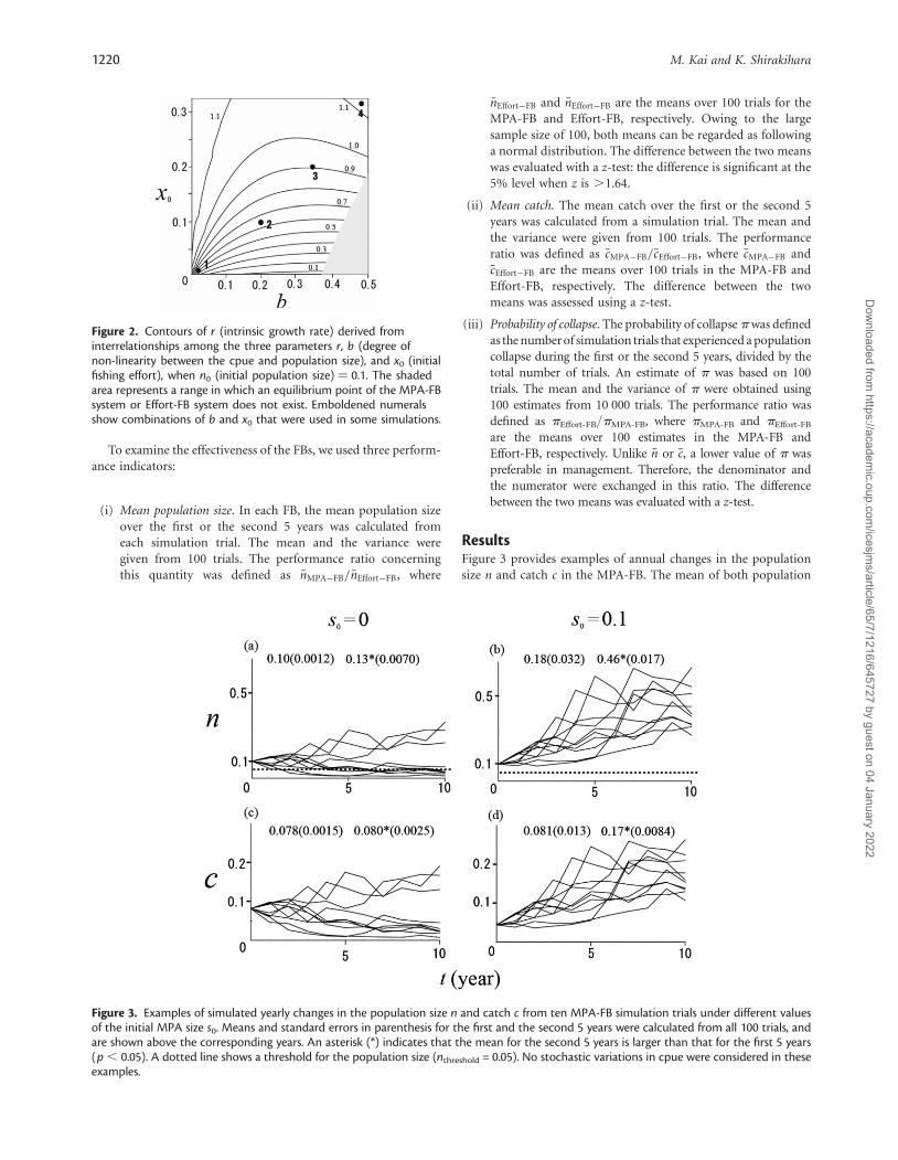
ResultsFigure 3 provides examples of annual changes in the populationsize n and catch c in the MPA-FB. The mean of both population

Figure 2. Contours of r (intrinsic growth rate) derived frominterrelationships among the three parameters r, b (degree ofnon-linearity between the cpue and population size), and x0 (initialfishing effort), when n0 (initial population size) ¼ 0.1. The shadedarea represents a range in which an equilibrium point of the MPA-FBsystem or Effort-FB system does not exist. Emboldened numeralsshow combinations of b and x0 that were used in some simulations.

Figure 3. Examples of simulated yearly changes in the population size n and catch c from ten MPA-FB simulation trials under different valuesof the initial MPA size s0. Means and standard errors in parenthesis for the first and the second 5 years were calculated from all 100 trials, andare shown above the corresponding years. An asterisk (*) indicates that the mean for the second 5 years is larger than that for the first 5 years(p , 0.05). A dotted line shows a threshold for the population size (nthreshold = 0.05). No stochastic variations in cpue were considered in theseexamples.


Dow


ic.oup.com/icesjm


size and catch was higher for the second 5 years than for the first 5years. However, in simulation trials (Figures 3a and c) and in trialswith n , nthreshold when s0 = 0 (when starting the MPA-FBwithout MPAs), a decreasing trend was observed in n or c. Suchphenomena were not observed in Figures 3b and d, when startingthe MPA-FB with the MPA size equal to 10% of the whole area (s0

= 0.1; Figures 3b and d). Annual changes in n and c were sensitiveto the initial MPA size s0. These were trials with n . ntarget (=0.5)in Figure 3b. This was caused by the oscillatory property of theequilibrium point. We confirmed the random fluctuations in naround ntarget based on simulations for more than 50 years.

Figure 4 shows the relationship between s0 and performancestatistics ( �n, �c, and p) in the MPA-FB. As expected from closingat least a part of the fishing grounds, �n increased with s0, and �nwas higher for the second 5 years than for the first 5 years(Figures 4a and b). The �c � s0 curves either monotonouslydecreased or were dome-shaped (Figures 4c and d). The lattershows that �c increased when s0 increased from 0 to the levelgiving the maximum value of �c. This level and �c were higher for

the second 5 years. The probability of collapse p decreasedsharply to almost 0 as s0 increased (Figures 4e and f), showingthat an adequate level of s0 prevented a population from collap-sing. The level was lower for the second 5 years.

Figure 5 shows the relationship between the CV (degree of sto-chastic variations in cpue) and the performance statistics for thefirst 5 years in the MPA-FB under two levels of s0. The mean ofboth population size �n and catch �c was not sensitive to changesin the CV (Figure 5a–d). The probability of collapse p increasedslightly with the CV when s0 = 0 (Figure 5e), but p was almost 0over the CV range of 0–200% when s0 = 0.1 (Figure 5f).

Figures 6–8 show performance ratios between the MPA-FB andEffort-FB systems under two different levels of s0. Domains of�nMPA�FB . �nEffort�FB or �nMPA�FB , �nEffort�FB appeared whens0 = 0 (Figure 6a and c), but domains of �nMPA�FB . �nEffort�FB

were overwhelmingly dominant when s0 = 0.1 (Figure 6b and d),showing that population recovery was accelerated more from theMPA-FB than from the Effort-FB. Figure 7 had domains of�cMPA�FB . �cEffort�FB or �cMPA�FB , �cEffort�FB. As the relationship

Figure 4. The relationship between s0 (initial MPA size) and performance statistics of n (mean population size), c (mean catch), and p(collapse probability) in the MPA-FB. Numbers, which correspond to those in Figure 2, represent combinations of b (degree of non-linearitybetween the cpue and population size) and x0 (initial fishing effort). No stochastic variations in cpue were considered in these simulation trials.


Dow


ic.oup.com/icesjm


between �cMPA�FB and s0 changed depending on the parametervalues (Figures 4c and d), an inconsistent relationship wasobserved between the ratio �cMPA�FB=�cEffort�FB and s0. Domains ofpMPA-FB , pEffort-FB or pMPA-FB . pEffort-FB appeared when s0 =0 (Figures 8a and c), but only pMPA-FB , pEffort-FB when s0 = 0.1(Figures 8b and d), showing that the MPA-FB was more effectivethan the Effort-FB in preventing the population from collapsing.

DiscussionOur stability analyses suggest that both the MPA-FB and Effort-FBcan approach a predetermined target level for a population whencpue is used instead of population size, and when the non-linearrelationship appears between cpue and population size. Thenecessary conditions are that (i) the target cpue is set at a levelcorresponding to the population size that provides MSY, and(ii) drastic changes in the MPA size or fishing effort are avoided.Condition (ii) may require many years for a depleted populationto approach a target level. A simple solution to cope with this dif-ficulty is that all fishing grounds be closed until the populationrecovers. However, this may not be accepted by fishers, especiallywhen they exploit a population with a low growth rate. The othersolution, which will be examined in future, is to develop a controlsystem for changing the MPA size or fishing effort more rapidly. Inthe present system, the changes are regulated by a constant h that

must be set at a very low value to make the system stable. If wecould assign a high h (to approach the target level rapidly) whenthe difference between the target and observed cpue is large, anda low h (to approach the target level slowly, without overshootingthe level) when the difference is small, recovery of a depletedpopulation could be accelerated.

Both FBs can contribute to preventing a depleted populationfrom collapsing if stochastic population fluctuations are indepen-dent of population size. Because both FBs can increase the popu-lation size, collapse probability is less when the population size islarger, although collapses did appear in some simulation trialsincorporating stochastic population fluctuations.

Our simulations, which focused on the system dynamics overthe short term after management implementation, showed thatthe performance of each FB depends on s0 (initial MPA size), x0

(initial fishing effort), and b (the degree of non-linearitybetween cpue and population size). We cannot make a generalcomment on whether one FB is always better than the other.When s0 = 0 (starting the MPA-FB from 0 MPAs), managementeffect is never remarkable because the MPA size increases onlyslowly because of a very low h. However, as suggested from simu-lations with s0 = 0.1, when s0 is set at an intermediate value, theperformance of the MPA-FB may improve. The MPA-FB cansave individuals in MPAs, whereas the Effort-FB allows fishers to

Figure 5. Relationship between the degree of stochastic variations in cpue, which is given by the CV (coefficient of variation), andperformance statistics of n (mean population size), c (mean catch), and p (collapse probability) in the MPA-FB. Numbers, which correspond tothose in Figure 2, represent combinations of b (degree of non-linearity between the cpue and population size) and x0 (initial fishing effort).Simulation trials were done for the first 5 years.


Dow


ic.oup.com/icesjm


use all fishing grounds. Simulations confirmed that the MPA-FBhas the advantage over the Effort-FB in preventing a depletedpopulation from collapsing. A trade-off may exist between rapidpopulation recovery and a high level of short-term catch.However, the trade-off will disappear when the MPA-FB succeedsin allowing the population to recover. A high catch can be expectedfrom a fully recovered population even when fishing effort isunchanged (fishing effort x in the MPA-FB was fixed at x0 insimulations).

The cpue may be variable even when the population size is con-stant. This will limit the advantages of the MPA-FB. However,simulations incorporating stochastic variations in cpue showedthat a population rarely collapses when s0 = 0.1.

Adopting the MPA-FB with a high level of s0 is a recipe forvariability in cpue. Although we cannot specify the level of s0

based on the present study, s0 = 1 (starting the MPA-FB fromthe closure of all fishing grounds) is an option for a heavilydepleted population, especially when the control system for accel-erating population recovery will be applicable. For a lightlyexploited population with low variability in cpue, s0 = 0 is anoption, although no simulation studies for such a populationwere performed here. It is advisable that a given level of s0 beput in place before implementing this FB.

In our simulations, only the population characteristics r(intrinsic growth rate) and b were considered to affect the per-formance of the two FBs. To compare their performance, we

Figure 6. Contours of nMPA-FB/nEffort-FB (ratio of mean population sizes) in the plane of b (degree of non-linearity between the cpue andpopulation size) and x0 (initial fishing effort). Numbers in rectangles represent values of nMPA-FB/nEffort-FB. Figure 2 is overlaid. A legend ofnMPA-FB . nEffort-FB (p , 0.05) indicates that nMPA-FB was larger than nEffort-FB at the 5% level of significance. No stochastic variations in cpuewere considered in these simulation trials.


Dow


ic.oup.com/icesjm


could not change the values of these parameters independently.Instead, we changed combinations of r and b, where r wasdetermined uniquely from a combination of b and x0 (seeFigures 6–8). However, irrespective of b, i.e. even when b washigh and hyperstability appeared, we saw a better performanceof the MPA-FB than the Effort-FB when r was high. In thepresent control system, with a constant and low h, the MPA-FBwould be effective for a population that can recover quickly byitself because it has a high r.

For technical reasons, the specific models cannot deal withhyperdepletion (Hilborn and Walters, 1992), corresponding toa . 1 in Uexpected / Na. However, the basic models can handleit. Stability analyses using them suggest that the dynamicsystems are globally stable even when a . 1. Therefore, our

feedback management procedure can recover a depleted popu-lation even in a case of hyperdepletion.

Management effectiveness using MPAs depends on the mobi-lity of the target species (Polachek, 1990; DeMartini, 1993;Sladek-Nowlis and Bollermann, 2002; Botsford et al., 2003;Moustakas et al., 2006). As suggested from the specific modelsused for our simulations, we allowed for the relationshipbetween MPA size and the catch expected from a density-dependent spatial distribution pattern (Kai and Shirakihara,2005), but we did not consider mobility explicitly. Therefore, wecannot examine differences in the effect between highly migratoryspecies and sedentary species. However, temporal removal ofMPAs is unlikely to be feasible for highly mobile species becauselarger areas are needed for the MPA to achieve benefit as the

Figure 7. Contours of cMPA-FB/cEffort-FB in the b2x0 plane. Numbers in rectangles represent values of cMPA-FB/cEffort-FB. Figure 2 is overlaid. Alegend of cMPA-FB . cEffort-FB (p , 0.05) indicates that cMPA-FB was larger than cEffort-FB at the 5% level of significance. No stochastic variationsin cpue were considered in these simulation trials.


Dow


ic.oup.com/icesjm


rates of movement increase (Polachek, 1990; Sladek-Nowlis andBollermann, 2002).

A difficulty in the MPA-FB based on cpue is that the cpueevaluated from commercial catch–effort statistics has no infor-mation on abundance within MPAs, so may not reflect the abun-dance of the whole population. Ad hoc measures, such astemporal removal of MPAs before the fishing season of eachyear (i.e. preseason), could be applied. Preseason fishing shouldbe implemented carefully to avert serious damage to the depletedpopulation.

The usefulness of the MPA-FB should be evaluated withcaution. In a real world, variations in population size may bemore complex than simple stochastic variations independent ofsize. The relationship between size and cpue may be time-dependent. Continuous changes in the MPA size are never feasiblefor real populations. In future, we will focus on coastal sedentaryspecies, which are suitable for implementation of the MPA-FB in

that (i) spatial distributions and annual fluctuations are morereadily grasped than migratory species, (ii) the movement costfor the preseason fishing is relatively low, and (iii) low mobilityyields advantages to protect individuals in the MPA. We hope todevelop a practical rule for these species, by varying the MPAsize with annual changes in cpue.

AcknowledgementsWe thank K. Hiramatsu, K. Tatsukawa, T. Katsukawa, A. Moriyama,and the members of the Fish Population Dynamics Laboratory ofthe Ocean Research Institute in Tokyo University for their valuedcomments and suggestions, along with those from the editorand two anonymous referees. The study was supported by aGrant-in-Aid for Scientific Research (No.12NP0201) and the 21stCentury COE Programme of the Ministry of Education, Culture,Sport, Science, and Technology, Japan.

Figure 8. Contours of pEffort-FB/pMPA-FB in the b –x0 plane. Numbers in rectangles represent values of pEffort-FB/pMPA-FB. Figure 2 is overlaid.A legend of pMPA-FB, pEffort-FB (p , 0.05) indicates that pMPA-FB was smaller than pEffort-FB at the 5% level of significance. No stochasticvariations in cpue were considered in these simulation trials.


Dow


ic.oup.com/icesjm


ReferencesBotsford, L. W., Micheli, F., and Hastings, A. 2003. Principles for the

design of marine reserves. Ecological Application, 13: 25–31.

Bulmer, M. 1994. Theoretical Evolutionary Ecology. SinauerAssociates, Sunderland, MA. 400 pp.

Clark, C. W. 1982. Concentration profiles and the production andmanagement of marine fisheries. In Economic Theory of NaturalResources, pp. 97–112. Ed. by W. Eichhorn, R. Henn, K.Neumann,, and R. W. Shephard. Physica-Verlag, Wurzburg,Germany. 645 pp.

DeMartini, E. E. 1993. Modelling the potential for fishery reserves formanaging Pacific coral reef fishes. Fishery Bulletin US, 91: 414–427.

Guenette, S., and Pitcher, T. J. 1999. An age-structured model showingthe benefits of marine reserves in controlling overexploitation.Fisheries Research, 39: 295–303.

Harada, Y., Sakuramoto, K., and Tanaka, S. 1992. On the stability ofthe stock-harvesting system controlled by a feedback managementprocedure. Research on Population Ecology, 34: 185–201.

Harley, S. J., Myers, R. A., and Dunn, A. 2001. Is catch-per-unit-effortproportional to abundance? Canadian Journal of Fisheries andAquatic Sciences, 58: 1760–1772.

Hastings, A., and Botsford, L. W. 1999. Equivalence in yield frommarine reserves and traditional fisheries management. Science,284: 1537–1538.

Hilborn, R., and Walters, C. J. 1992. Quantitative Fisheries StockAssessment: Choice, Dynamics & Uncertainty. Chapman andHall, London. 570 pp.

Jones, P. J. S. 2002. Marine protected area strategies: issues, divergencesand the search for middle ground. Reviews in Fish Biology andFisheries, 11: 197–216.

Kai, M., and Shirakihara, K. 2005. A feedback management procedurebased on controlling the size of marine protected areas. FisheriesScience, 71: 56–62.

Karagiannakos, A. 1996. Total Allowable Catch (TAC) and quota man-agement system in the European Union. Marine Policy, 20: 235–248.

Moustakas, A., Silvert, W., and Dimitromanolakis, A. 2006. A spatiallyexplicit learning model of migratory fish and fishers for evaluatingclosed areas. Ecological Modelling, 192: 245–258.

Pella, J. J., and Tomlinson, P. K. 1969. A generalized stock productionmodel. Inter-American Tropical Tuna Commission Bulletin, 13:421–458.

Polachek, T. 1990. Year-round closed areas as a management tool.Natural Resource Modelling, 4: 327–354.

Rodwell, L. D., and Roberts, C. M. 2004. Fishing and the impact ofmarine reserves in a variable environment. Canadian Journal ofFisheries and Aquatic Sciences, 61: 2053–2068.

Shirakihara, K., and Tanaka, S. 1978. Two fish species competitionmodel with non-linear interactions and equilibrium catches.Research on Population Ecology, 20: 123–140.

Sladek-Nowlis, J., and Bollermann, B. 2002. Methods for increasingthe likelihood of restoring and maintaining productive fisheries.Bulletin of Marine Science, 70: 715–731.

Sladek-Nowlis, J., and Roberts, C. M. 1999. Fisheries benefits andoptimal design of marine reserves. Fishery Bulletin US, 97:604–616.

Tanaka, S. 1980. A theoretical consideration on the management of astock-fishery system by catch quota and on its dynamical proper-ties. Bulletin of the Japanese Society of Scientific Fisheries, 46:1477–1482.

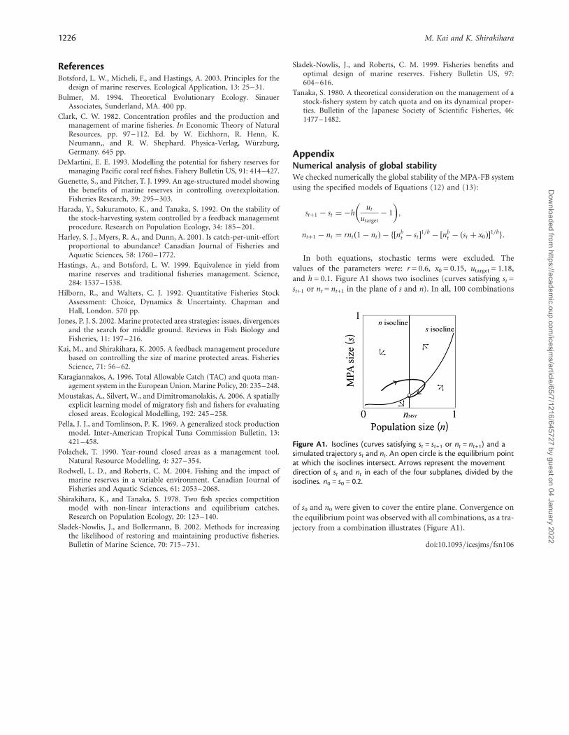
AppendixNumerical analysis of global stabilityWe checked numerically the global stability of the MPA-FB systemusing the specified models of Equations (12) and (13):

stþ1 � st ¼ �hut

utarget� 1

� �;

ntþ1 � nt ¼ rntð1� ntÞ � f½nbt � st �

1=b � ½nbt � ðst þ x0Þ�

1=bg:

In both equations, stochastic terms were excluded. Thevalues of the parameters were: r = 0.6, x0 = 0.15, utarget = 1.18,and h = 0.1. Figure A1 shows two isoclines (curves satisfying st =st+1 or nt = nt+1 in the plane of s and n). In all, 100 combinations

of s0 and n0 were given to cover the entire plane. Convergence onthe equilibrium point was observed with all combinations, as a tra-jectory from a combination illustrates (Figure A1).

doi:10.1093/icesjms/fsn106

Figure A1. Isoclines (curves satisfying st = st+1 or nt = nt+1) and asimulated trajectory st and nt. An open circle is the equilibrium pointat which the isoclines intersect. Arrows represent the movementdirection of st and nt in each of the four subplanes, divided by theisoclines. n0 = s0 = 0.2.


Dow


ic.oup.com/icesjm


Date post:	11-Feb-2022
Category:	Documents
Upload:	others
View:	2 times
Download:	0 times

Effectiveness of a feedback management procedure based on

Documents