{Y\ ,)-\o[)12- qTISv Southwest Region University Transportation Center Effectiveness of Accelerating Highway Rehabilitation in Urban Areas SWUTC/95/60058-1 Center for Transportation Research University of Texas at Austin 3208 Red River, Suite 200 Austin, Texas 78705-2650
Transcript
{Y\ ,)-\o[)12-
qTISv Southwest Region University Transportation Center
Effectiveness of Accelerating Highway
Rehabilitation in Urban Areas
SWUTC/95/60058-1
Center for Transportation Research University of Texas at Austin
3208 Red River, Suite 200 Austin, Texas 78705-2650
1. Report No. 2. Government Accession No.
SWUTC/95/6OO58-1 4. Title and Subtitle
Effectiveness of Accelerating Highway Rehabilitation in Urban Areas
7. Aulhor(s)
Eduardo Trujillo Olguin, Brent T. Allison, and B. Frank McCullough
9. Performing Oxganization Name and AddreBB
Center for Transportation Research University of Texas at Austin 3208 Red River, Suite 200 Austin, Texas 78705-2650
12. Sponsoring Agency Name and AddreBB
Southwest Region University Transportatio Texas Transportation Institute The Texas A&M University System College Station, Texas 77843-3135
IS. Supplementary Notes
"jiilln,flf L021090
3
S. Report Date
March 1995 6. Perfonning OrJanization Code
8. Perfonning OrJanization Report No.
Research Report 60058-1
10. Work Unit No. (TRAIS)
11. Contract or Grant No.
0079
14. Sponsoring Agency Code
Supported by a grant from the Office of the Governor of the State of Texas, Energy Office 16. Abstract
onPa e
The purpose of this research report is to establish guidelines for identifying highway rehabilitation projects warranting acceleration within Texas. Reduction in the total number of days allocated for project completion is recommended if savings in user costs are greater than the additional costs of accelerating the project. Throughout this report, the short-term impacts to road users and the environment were analyzed, and methods for quantifying user costs were reviewed. The potential consequences of accelerating rehabilitation projects were also presented. A methodology to estimate additional construction costs was developed to assess the effectiveness of accelerated construction schedules. Finally, recommendations are made to identify candidates within the Texas Highway system for expediting highway rehabilitation by means of threshold traffic volumes warranting project acceleration.
17. Key Words
Pavement Acceleration, Rehabilitation, Urban Highways, Expediting, Impact Studies, User Costs, Traffic Modeling, Conventional vs. Accelerated
18. Distribution Statement
No Restrictions. This document is available to the public through NTIS: National Technical Information Service 5285 Port Royal Road Springfield, Virginia 22161
19. Security Classif.(oflhis report)
Unclassified 20. Security Classif.(ofthis page) 21. No.ofPageB I 22. Price
Unclassified 169 Fonn DOT F 1700.7 (8-72) Reproduction of completed page authorized
EFFECTIVENESS OF ACCELERATING
HIGHWAY REHABILITATION
IN URBAN AREAS
by
Eduardo Trujillo Olguin, Brent T. Allison, and B. Frank McCullough
Research Report SWUTC 60058-1
Research Project 60058
Energy Consumption Related to Excessive User-Delay During Highway Rehabilitation
conducted by the
CENTER FOR TRANSPORTATION RESEARCH
Bureau of Engineering Research
THE UNIVERSITY OF TEXAS AT AUSTIN
March 1995
ii
ABSTRACT
The purpose of this research report is to establish guidelines for identifying highway
rehabilitation projects warranting acceleration within Texas. Reduction in the total number of
days allocated for project completion is recommended if savings in user costs are greater than
the additional costs of accelerating the project. Throughout this report, the short-term impacts
to road users and the environment were analyzed, and methods for quantifying user costs were
reviewed. The potential consequences of accelerating rehabilitation projects were also
presented. A methodology to estimate additional construction costs was developed to assess
the effectiveness of accelerated construction schedules. Finally, recommendations are made
to identify candidates within the Texas Highway system for expediting highway rehabilitation
by means of threshold traffic volumes warranting project acceleration.
ACKNOWLEDGEMENTS
This publication was developed as part of the University Transportation Centers Program
which is funded 50% in oil overcharge funds from the Stripper Well settlement as provided by
the Texas State Energy Conservation Office and approved by the U.S. Department of Energy.
Mention of trade names or commercial products does not constitute endorsement or
recommendation for use.
iii
EXECUTIVE SUMMARY
This research· effort was conducted in order to examine the energy consumption related
to excessive user delay during highway rehabilitation. Under certain circumstances the
acceleration of highway rehabilitation can be a benefit, in terms of energy, time, and production
costs to the citizens of Texas. The purpose of this research report is to present guidelines that
help to identify candidates for accelerated highway rehabilitation strategies.
This will be accomplished by examining the short-term impacts generated by highway
rehabilitation on the several parties impacted by the rehabilitation process. Because these
impacts are a function of the traffic-handling techniques used, a review of common types of work
zones is also presented. Next, a review of the existing methodologies used to quantify the
adverse impacts on road users from highway rehabilitation will be examined. The resulting data
is then used in economic analyses of alternatives. The next section is concerned with
acceleration strategies that mitigate the impacts generated by rehabilitation activities. An
examination of the several potential consequences of accelerating rehabilitation projects is
presented. This analysis is focused on determining how the cost of the project is affected by
acceleration. There is also a methodology established for evaluating the effectiveness of
accelerating rehabilitation projects as a mitigation measure for total user costs and fuel
consumption. This methodology, presented in the former chapter, is applied to a factorial
experiment. Guidelines for identifying projects warranting acceleration are developed in this from
this. Finally, conclusions and recommendations are presented in the final chapter.
As the U.S. Interstate Highway Program nears completion, and as vehicular traffic
continues to grow in urban areas, state and national highway officials must increasingly turn their attention away from the building of new facilities to the rehabilitation of older ones (Ref
1.1). The need for improvements is likely to continue well beyond the year 2000 for more
than 40 percent of the Interstate highways and for about 70 percent of the arterials (Ref 1.2). Unfortunately, highway rehabilitation activities undertaken on Texas' major freeways,
especially in urban areas, create temporary negative impacts on road users, adjacent
property owners, and the environment. Highway users are affected by increased travel times
and operating costs resulting from excessive delays, as well as the need to reduce vehicular speeds within the construction site. At the same time, property owners often experience a
reduction in business revenues owing to restricted or inconvenient access to their businesses. And finally, the increased congestion and fuel consumption resulting from construction delays can compromise air quality through a concomitant increase in tailpipe emissions.
Construction activities can also adversely impact the supervising highway agency -especially when traffic operations must be maintained during the project. If the agency,
represented in Texas by the Texas Department of Transportation, does a poor job of handling the conflicts between construction activities and traffic operations, then the agency's
credibility with the public can be impaired. And contractors may lose efficiency and productivity because of a lack of space for construction operations (Ref 1.3).
Because of their ostensible convenience and their array of abutting commercial development, Texas' urban freeways typically carry large volumes of traffic. During rehabilitation projects, competition for space takes place between traffic operations and construction activities. When a limited right of way exists, the faCilities under rehabilitation
experience severe congestion, even if only a small portion of the road is temporarily closed. The Texas Department of Transportation has recognized that the initial cost of
construction, along with the ongoing maintenance costs, is not the only budgetary considerations involved in selecting the best alternative for rehabilitation projects. Highway user costs, including vehicle operating costs, travel time costs, and accident costs, must be considered when total life-cycle cost analyses are used to evaluate rehabilitation alternatives (Ref 1.4). The costs of improving the highway network are usually justified by the long-term benefits that accrue to road users and to the community. Reduced vehicle operating costs,
reduced travel times, enhanced economic development, and increased property values are
among the long-term benefits. However, special attention must be given not only to long-term benefits for road
users and the community, but also to those temporary negative impacts associated with
1
construction activities. The severity of these short-term impacts on users, property owners,
and the environment is related to (1) the traffic volumes disrupted while the facility is under
rehabilitation, and (2) the duration of such disruption. As shown in Figure 1.1, highway user
costs increase during rehabilitation and reconstruction operations. These user costs are the
sum of three main components: vehicle operating costs, user travel-time costs, and accident
costs. Even though highway improvements reduce long-term user costs, potential temporary
increases in congestion, fuel consumption, and vehicle emissions can be extremely
significant if available measures to mitigate such negative impacts are not applied at the right
time or to the proper extent.
USER COST
REHABILITATION PROJECT DURATION ...
BEFORE
TIME
AFTER
Figure 1. 1. Highway user costs affected by rehabilitation activities (Ref 1.5).
Other negative impacts (in addition to increased user costs) also vary in accordance with the duration of the project and the traffic handling strategy used during highway
rehabilitation. Potential negative effects of highway rehabilitation activities, which have been identified in past research (Refs 1.1, 1.3), are summarized as follows:
a) Increased vehicle operating costs, including increased fuel consumption as a result of excessive idling, stop-and-go driving conditions, and longer alternative routes.
b) Increased user-delay costs resulting from induced congestion.
c} Increased safety costs (both for traffic handling requirements and increased likelihood of accidents).
d) Increased environmental costs (i.e., the air pollution that results from excessive vehicle emissions during congested periods).
e) Constrained access to adjacent commercial property that reduces potential revenue earnings during the construction period.
f) Interference with third parties, such as utility owners or delivery companies. whose services might be restricted by construction activities.
2
There are techniques to quantify some of the negative effects of rehabilitation, including user delays, fuel consumption, and vehicle emissions. To mitigate other negative impacts, such as a loss of business by adjacent commercial property, researchers must rely on subjective evaluations of local experience (Ref 1.3). There are two common practices used for mitigating the negative effects of highway rehabilitation activities. The first of these
practices involves avoiding conflicts between construction activities and traffic operations by
conducting construction during low-demand periods or by diverting traffic to other routes.
The second most common practice used for expediting construction involves reducing the
duration of the project and, thus, diminishing the temporary negative effects caused by the rehabilitation (Ref 1.3).
Project duration affects the total project cost, since user costs and the administrative costs increase linearly with time, while the construction costs increase as the duration of construction is reduced (Ref 1.4). Figure 1.2 shows the effect of project duration on the total project cost.
mOH
LOW
/ / - -
Minimum Total Project Cost
/ /
/ /Minimum
First Cost
User Costs
Construction Cost + Administration Cost
-r--__ Construction Cost
- AdministJation Cost ----Duration of Construction
Figure 1.2. Effect of project duration on the total project cost (Ref 1.4).
1.2 OBJECTIVE OF STUDY
Research study 60058, "Energy Consumption Related to Excessive User Delay During Highway Rehabilitation," was conducted in order to analyze the relationship between the excess fuel consumption resulting from highway rehabilitation in Texas and the increased construction costs resulting from expediting the entire construction schedule. If the costs associated with the energy wasted by motorists idling on the freeway could be quantified, the
cost of modifying the construction schedule might be justified and, thus, be a great benefit to
the citizens of the state. The study has the following objectives:
1 . For various traffic levels, estimate both the quantity and costs of fuel consumed by motorists experiencing excessive travel delays caused by highway rehabilitation.
3
2. For identical construction scenarios and traffic levels, estimate the additional construction costs that would be incurred if congestion was expedited and/or forced to off-peak hours.
3. Compare the costs identified in objectives 1 and 2 and then, using the results, develop guidelines for engineers to follow when developing construction schedules.
4. Determine the feasibility of incorporating these guidelines in a computer model that could be used by engineers to balance the trade-off between energy consumed during user delays and the cost of modifying the construction schedule.
Increased fuel consumption, however, is only one of several negative impacts
caused by highway rehabilitation activities. In highly trafficked corridors, highway
rehabilitation can result in excessive user delays, increased vehicle operating costs, potential
accidents for both motorists and working crews, increased tailpipe emissions from vehicles,
and potential loss of revenues to adjacent businesses.
The temporary negative impacts of rehabilitation projects rise in proportion to the traffic that uses the facility. The more traffic volume expected to use the facility, the higher the cost per day of such negative impacts. These negative effects increase excessively at a
certain level of traffic, necessitating the acceleration of the rehabilitation project. The
following graph shows the relationship between traffic volumes (ADT) and daily costs of negative impacts resulting from rehabilitation activities. These costs are a function of the traffic volumes, hourly traffic distribution, traffic composition, speed of vehicles approaching
and passing through the work zone, the work zone configuration, and the number of hours of
actual work.
Cost Per Day
$ Total User Costs: a) Time delays b) Op:rtating costs c) Accilents
User Tolerance Level d) Emissions
Expediting .. Traffic \b lumes (ADT)
Figure 1.S. Relationship between traffic volumes (ADT) and daily costs
of negative impacts due to rehabilitation activities.
Highway users, however, are not willing to accept increased travel costs and delays
for long periods of time or over a certain dollar amount. Because the degree of tolerance that highway users may accept varies from one project to another, estimates of user tolerance are based on intuition conditioned by local experience (Ref 1.3). These levels of
4
tolerance also apply to the rate of vehicle emissions that can be allowed before expediting of the construction process becomes imperative.
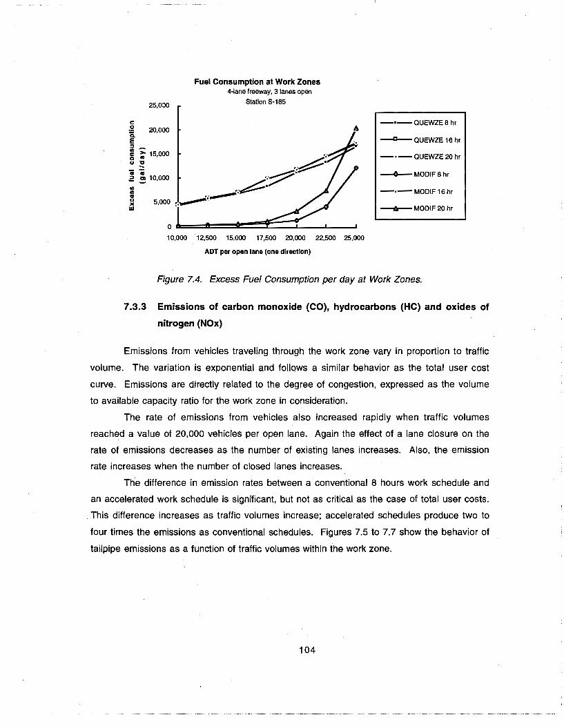
The number of days for significant user and environmental costs to accumulate is directly related to the amount of traffic traveling through construction zones (Figure 1.4). Therefore, if acceptable user and environmental costs could be established, the number of
days within the tolerance level could be determined. As a result, rehabilitation projects
lasting longer than the number of days within the tolerance level for user and environmental
costs require the implementation of expediting construction strategies.
Cumulative Costs $
User Thlerance Level
I Ex. pediting
I Thres:ld 2
N umber of days
Figure 1.4. Relationship between traffic volumes and the number of days
required to reach tolerance in user and environmental costs.
The purpose of this research report is to document the development of guidelines to identify suitable projects warranting implementation of accelerated construction schedules
within Texas. Accelerating highway rehabilitation could be justified by comparing existing traffic volumes with those given in the guides as the minimum volumes required before
expediting construction is recommended. In this fashion, the cost of expediting construction can be justified by the reduced negative impacts to road users and the environment, if the
expect~d traffic volumes are greater than those provided in the guides for a range of work zone configurations.
1.3 REPORT ORGANIZATION
This research report consists of eight chapters. Chapter 1 is the introductory chapter. Chapter 2 describes the short-term impacts of highway rehabilitation projects on the several parties involved, including those who use the facility or are serviced by it. Because these
impacts are a function of the traffic-handling techniques used, a review of common types of
work zones is also presented. Chapter 3 deals with existing methodologies used to quantify
the adverse impacts on road users from highway rehabilitation; the resulting data are then
used in economic analyses of alternatives. Chapter 4 is concerned with strategies that
mitigate those impacts generated by rehabilitation activities. Chapter 5 analyzes several
5
potential consequences of accelerating rehabilitation projects. This analysis focuses on
determining how the cost of the project is affected by acceleration. Chapter 6 establishes a methodology for evaluating the effectiveness of accelerating rehabilitation projects as a
mitigation measure for total user costs and fuel consumption. Chapter 7 applies the
methodology presented in the former chapter to a factorial experiment. Guidelines for
identifying projects warranting acceleration are developed in this chapter. Finally, conclusions
and recommendations are presented in Chapter 8.
1.4 REFERENCES
1.1. Long, R. B. (1991). Expediting Pavement Construction in Urban Areas, Master's thesis,
University of Texas at Austin.
1.2. Leathers, R. C. (1987), "FHWA Perspectives: A Comprehensive Approach to Major
Highway Reconstruction Projects," Transportation Management for Major Highway
Reconstruction. Transportation Research Board Special Report 212. Washington,
D.C.
1.3. Ward, W. V., and B. F. McCullough (1993). Mitigating the Negative Effects of Urban Highway Construction, Research Report 1227-1F, Center for Transportation Research, The University of Texas at Austin.
1.4. de Solminihac, H. (1991). "Expediting Pavement Construction," Presentation at XX
Seminario de Ingenieria de Transito, Mexico D.F.
1.5. Suliman, M. R. (1993). Expediting Strategies to Mitigate the Adverse Effects of
Pavement Construction in the State of Texas, doctoral dissertation, The University of
Texas at Austin.
6
CHAPTER 2, SHORT-TERM IMPACTS FROM HIGHWAY REHABILITA1'ION IN URBAN
AREAS
2,1 BACKGROUND
Higher traffic volumes and heavier vehicles have increased highway network deterioration. Unfortunately, the sections of the highway system suffering the most are those associated with high mobility and heavy traffic, and whose infrastructures are rapidly aging.
Therefore, many of these sections require major rehabilitation and reconstruction to preserve
the integrity of the syst~m. Moreover, most of the major freeways in large urban areas
already operate under saturated conditions for long periods every day. Consequently,
furnishing adequate space for reconstruction activities, while minimizing delays and property
inaccessibility, is a challenging task for transportation agencies (Ref 2.1).
Highway rehabilitation and reconstruction commonly require a minimum of several weeks and may involve multiple construction seasons. A basic characteristic of long-term work zones is that traffic control strategies must (1) accommodate both daytime and
nighttime conditions, and (2) provide a safe and expeditious traffic flow throughout the conflict zone. The type of traffic control adopted for a specific rehabilitation project has been dependent on the work involved and regulated by uniform standards and guidelines (e.g.,
the Manual on Uniform Traffic Control Devices). The main purpose of such traffic control standards is to enhance safety at work zones, both for road users and work crews. The
magnitude of the short-term negative impacts of highway rehabilitation projects on road
users and adjacent businesses (including user delays, increased operating costs, and
emissions from vehicles), depends on the type of traffic control as well as on the duration of the project.
The common practice of adapting traffic to the work zone by establishing a standard
traffic control plan is becoming obsolete for major travel corridors in urban areas. A different approach must be established in these corridors, one in which the work zone is adapted to the traffic conditions (Ref 2.4). Alternative traffic control strategies must be analyzed to
identify the one that generates the least impact on users and adjacent businesses. Also the issue of safety comes into play in areas with high volumes of traffic. The most common traffic control strategies for highway rehabilitation are summarized below.
2.2 TRAFFIC HANDLING TECHNIQUES
In urban environments, there are alternative ways for securing a portion of the roadway when conducting reconstruction activities. Closures may involve a shoulder, one or
more lanes, a whole direction of the highway, or even the entire highway. Heavy traffic
demands on urban freeways, however, prevent the use of dramatic closures, given that
traffic operations must be maintained throughout the rehabilitation work. The most common
7
closure strategies related to highway rehabilitation activities include lane closures, lane alterations, median crossovers, and detours (Refs 2.3, 2.4, 2.7).
2.2.1 Lane closure
A lane closure forces the traffic stream to merge into another lane (leaving the closed lane). Because this strategy reduces the total number of lanes, a careful analysis is
recommended to determine whether serious congestion and delays will result from the lane
closure. Closing an auxiliary lane, such as a turn bay or a deceleration lane approaching an off ramp, is not considered a lane closure, since the number of available lanes is not reduced.
On multilane facilities, more than one lane may need to be closed to conduct the
required rehabilitation work. If two or more lanes are to be closed, a common practice is to close them one at a time, leaving a minimum length between each closure for speed
reduction and merging operations. If the work zone is located on a central lane of a multilane facility, it is recommended that the adjacent outer lane be closed to avoid an island
situation. Figure 2.1 shows a lane closure .
....
.... ...
... ...
Figure 2.1. Lane closure.
2.2.2 Lane Alteration
Lane alteration is another method for. providing space for rehabilitation activities on urban freeways. The basic premise of lane alterations is to keep the maximum number of open lanes through the conflict area, reducing potential disruptions to traffic. Lane alteration
involves the lateral displacement of one or more traffic lanes from their normal alignment in
order to accommodate a rehabilitation work zone. In this type of closure, usually all lanes are carried through and no merging operations are involved. Lane narrowing, use of shoulder or
median, and adding temporary lanes are means of establishing lane alterations.
Lane Narrowing. This type of lane alteration is configured by reducing the width of
those lanes carried through the work area. The maximum number of open lanes is maintained on the remaining space once the work zone has been delineated. The minimum
8
lane widths that must be provided depend on the type of facility and on the length of the work zone (Ref 2.4). Table 2.1 summarizes the minimum lane widths that must be provided with narrow lanes.
Minimum lane width (ft)
Type of facility Passenger cars Mixed Traffic only
Divided 3.5 - 5.5 miles 10.5 11 Divided 5.5 - 9 miles 11.5 11
Divided> 9 miles 12 12 Contra-flow lanes 10 11
Table 2.1 Minimum lane width according to the type of facility (Ref 2.4).
Also, a minimum clearance between the edge of the temporary lane and the work area itself must be provided, usually 2 to 3 ft. Figure 2.2 illustrates a lane-narrowing closure strategy.
- -- - - - - - -- -...
Figure 2.2 Lane narrowing.
Use of shoulder or median. This strategy involves the use of shoulders or the median as a temporary traffic lane. When using this kind of alteration, it is necessary to ensure that the shoulder or the median surface will adequately support the expected traffic
loads, and that the traffic can travel safely through the temporary lane. It is important to
keep the heavy loads from truck traffic off the inside shoulder, to avoid excessive damage on the permanent pavement structure. Whenever lane layout is altered to carry traffic in other parts of the roadway, appropriate geometric characteristics, such as turning radii, should be
9
provided for the speeds at which temporary lanes are to be traveled. Some examples of this technique are shown in Figure 2.3.
Adding temporary lanes. This type of work zone consists of rerouting traffic to a
temporary roadway constructed within the existing right of way, usually by widening the
original cross section. This strategy requires extensive preparation of the temporary roadway in order to support the traffic loads. Frequent maintenance is also needed to ensure a safe
operation. Generally, in urban areas, space is no longer available to implement such a traffic
control alternative. Figure 2.4 illustrates this work zone strategy .
In this work zone scheme, traffic traveling in the direction where disruption occurs is
routed across a median to the opposite traffic lanes. Traffic carried diagonally across the
median into the other direction can be partial or full. In the case of partial crossover, only a
fraction of the traffiC is diverted, while the remaining vehicles continue to use the disturbed
roadway. Full median crossover means that a/l traffic is diverted to the opposite side in a
10
two-way operation. In any case, opposite traffic must be separated with barriers, drums, cones, or vertical panels throughout the length of the two-way operation.
The transition roadway used to divert traffic from one direction to the opposite must be equal to or better than the geometric standards of the permanent road. This kind of alternative might also be combined with other strategies. including lane narrowing or the use of shoulders, in order to maintain the same number of lanes. See Figure 2.5 for some
examples of median crossovers.
..... .... ...
Figure 2.5. Median crossover.
2.2.4 Detour
A detour is used to divert traffic to another facility in order to bypass the work site that, in this case, entails total closure of the roadway. This closure strategy is desirable when
there are underutilized routes running parallel to the main route. However, the strategy is not desirable in urban areas where the surrounding network, usually inferior to the main network,
is already saturated, and the extremely high volumes carried by the freeway cannot be
handled by smaller streets. Detour disadvantages include:
• Longer travel times as a result of longer routes and reduced speeds. • More delays and higher operating costs.
• Lower levels of service. • Higher accident rates than those at the work zone itself.
• Congestion and deterioration of alternative routes. • User confusion if adequate information is not provided.
In order to be acceptable by users, traffic detours require:
• That the substitute route be capable of handling the additional traffic.
• That drivers be well informed. • That the alternate route be thoroughly and clearly marked.
An example of a detour is shown in Figure 2.6.
11
...
Alternate Route
Figure 2.6. Detour.
Undesirable effects occurring during highway rehabilitation include congestion, safety
problems, limited property access, and high vehicle fuel consumption. These impacts on
existing traffic and economic activity need to be assessed during the project planning stage
(Ref 2.5). It is also necessary to find the best combination of two contradictory objectives:
conducting rehabilitation activities at a minimum cost, while reducing the negative impacts on
users and the economy. Closing the entire facility, or just one direction, so that construction
is unimpeded and motorists are not exposed to hazards, generates the least rehabilitation
cost. However, inadequate levels of service usually exist on alternate routes on major
corridors, so that traffic cannot be accommodated and unacceptable delays and increased
user costs result. A compromise must then be made between the two conflicting interests:
construction and traffic operations (Ref 2.5).
Several parties are affected by highway rehabilitation projects, including road users,
adjacent businesses, transportation agencies, contractors, and third-parties. The impacts
generated by the rehabilitation activities on each party are identified below:
2.3 IMPACTS ON ROAD USERS
Highway users include all of those who may be using any portion of the highway
right-of-way and its immediate environs (e.g., vehicle operators and their passengers). The
increase in the cost of travel resulting from highway rehabilitation disruptions is the primary concern of highway users. By far the greatest concern to road users is the increase in travel
time resulting from the slower speeds required while passing through the work zone (or the
additional travel time associated with traveling on alternate routes if diversion of traffic
occurs).
Slower speeds and longer travel distances also give rise to changes in vehicle
operating costs. Although the additional expenditure in fuel consumption, oil consumption,
vehicle maintenance, tire wear, and depreciation may not be noticed by road users, they
represent an economic loss for the community as a whole. Moreover, local, regional, and
12
national transportation goals may be jeopardized by the accumulated effects of highway rehabilitation; for example, energy conservation goals may not be attained if fuel is wasted in queues generated by rehabilitation activities.
In addition, the number and severity of accidents may increase as a result of the
presence of a work zone. For example, the extra travel on diversion routes may lead to an accident rate greater than that associated with. the work zone itself.
These three cost components - travel time, vehicle operating costs, and safety -
are used to assess the impacts of highway rehabilitation projects on road users. The
methodology for estimating the increase in the cost of travel is presented in the next chapter.
2.4 IMPACTS ON BUSINESSES
Businesses that depend on passing traffic and, consequently, convenient property
access are attracted to major transportation corridors. These types of businesses are concerned about potential losses in sales caused by reduced or inconvenient customer access resulting from rehabilitation activities. Property owners are also concerned about the extent to which reduced access will decrease the value of their ·property. In 1989 the Wisconsin Department of Transportation published a study analyzing the impacts of highway rehabilitation on businesses (Ref 2.6). Business impacts were assessed by surveying businesses adjacent to a number of reconstruction projects. This study concluded that the
overall level of business activity occurring during reconstruction operations declined an
average of 10 percent. Impacts on employment were less than the impacts on sales, since businesses were reluctant to lay-off full-time employees during a short-term decline in
business activity. The impact on adjacent businesses was related directly to the length of the
disruptions. The faster the project was completed, the less severe the impacts on business (Ref 2.6).
Loss of business and decline in property values resulting from highway rehabilitation, however, are difficult to quantify in a credible manner, since changes in the level of sales or
employment may be tied to factors other than the rehabilitation project. Therefore, impacts
on businesses must rely on subjective evaluations of local experience; accordingly, they are not typically included in economic analyses of rehabilitation alternatives (Ref 2.6).
2.5 IMPACTS TO THE TRANSPORTATION AGENCY
Transportation agencies are also affected in terms of economic and political interests. While the responsibility of the agency is to provide as many transportation services as available resources permit, the allocation of these resources for mitigating negative effects of
rehabilitation projects reduces the level of investment in permanent facilities. The
transportation agency, therefore, has two extreme courses of action. First, by providing extensive mitigation measures, the total number of completed projects may be reduced (or
proposals for projects may have to wait longer before approval). On the other hand, by not
13
providing mitigation measures, the agency may suffer a loss of esteem in the eyes of the
public (Ref 2.6).
2.6 IMPACTS ON CONTRACTORS
Contractors experience an increased element of risk when rehabilitating existing
highways (more so than when constructing entirely new facilities). The most common risks
are the unpredictability of costs associated with traffic handling and safety concerns,
conflicting utility services, access to adjacent property and the project site, third party
involvement, plan deficiencies, and atypical weather conditions. These risks are more likely
to be found within an urban environment, where there are greater volumes of traffic. In
addition, the need for transporting labor, supplies, and equipment throUgh adjacent traffic
can create conflicts that maybe resolved only by reducing either construction operations or
traffic operations. Contractors may fail to comply with required contract schedules (and face
financial losses) if they are unable to cope with these risks (Ref 2.6).
2.7 IMPACTS ON THIRD PARTIES
The impact of rehabilitation can also affect third parties. These third parties include
utility companies and parties using the highway facilities to serve other public interests (e.g.,
fire departments, law enforcement agenCies, public schools, public transit agencies, and
others). The interests of these parties may be affected by highway rehabilitation projects.
Utility companies, for example, may have facilities located within the highway right-of-way and
may have to reduce services during the reconstruction period in order to expedite the work.
The transportation agency must identify the affected parties and negotiate the necessary
agreements in order to coordinate the work of contractors with that of the third parties (Ref
2.6).
2.8 SUMMARY
This chapter focused on the qualitative assessment of temporary negative impacts of
highway rehabilitation on urban areas. These impacts are a function of the traffic handling
techniques applied to accommodate both the construction operations and traffic operations.
The most commonly used traffic handling strategies were reviewed and compared. Several
parties are involved in providing and using the highway network. The short-term impacts of
highway rehabilitation projects on road users, adjacent businesses and property owners,
transportation agencies, contractors, and third-parties were identified in this section.
2.9 REFERENCES
2.1. Burns, E. N. (1990). Managing urban freeway maintenance. National Cooperative Highway Research Program Synthesis of Highway Practice 170, Transportation Research Board, Washington, D.C.
14
T-
2.2. Transportation Research Board (1987). Transportation management for major highway reconstruction. Special Report 212. National Research Council, Washington, D.C.
2.3. Lewis, R. M. (1989). "Work zone traffic control concepts and terminology," Transportation Research Record 1230, Washington, D.C.
2.4. OECD Scientific Expert Group (1989). Traffic management and safety at highway work zones, Organization for Economic Cooperation and Development (OECD), Paris.
2.5. de Solminihac, H. E. (1991). "Expediting pavement construction," XX Semina rio de ingenieria de transito, Mexico D.F.
2.6. Ward, W. V., and B. F. McCullough (1993). Mitigating the effects of urban highway construction, Research Report 1227-1F, Center for Transportation Research, The University of Texas at Austin.
2.7. Abrams, C. M., and J. J. Wang (1981). Planning and scheduling work zone traffic control, Implementation package FHWA-IP-81-6. U.S. Department of Transportation, San FranCisco.
15
16
CHAPTER 3. ESTIMATION OF ADVERSE IMPACTS ON ROAD USERS FROM HIGHWAY
REHABILITATION
3.1 BACKGROUND
An economic analysis of potential rehabilitation alternatives must consider a number
of indirect costs that are related to the road user. The selected rehabilitation strategy must
provide benefits to road users over the service life (by means of lower travel costs resulting
from smoother and safer facilities) that outweigh the cost of the rehabilitation. The strategy
must also minimize the temporary increases in user costs resulting from the rehabilitation
itself.
The adverse impacts on road users resulting from highway rehabilitation can be
reduced by two general approaches: first, by implementing a range of mitigation strategies
during the rehabilitation project, and, secondly, by adopting a rehabilitation alternative that
may reduce the number of rehabilitation cycles (i.e., a more durable rehabilitation method).
In order to conduct an economic evaluation of alternatives, researchers should
estimate the adverse impacts on road user costs resulting from disruptions to traffic during
highway rehabilitation. User costs are a function of traffic volumes, road geometry, time and
duration of the rehabilitation work, the geometry of the work zone, and traffic management
techniques implemented (Ref 3.1).
3.2 OVERVIEW OF STUDIES IN ROAD USER COSTS
Studies on the cost of operating motor vehicles were initiated in the United States
soon after World War I by Agg (1923), who studied the performance of a small fleet fitted
with fuel flowmeters (Refs 3.2, 3.4). This study reported fuel consumption as a function of
speed and initiated a series of vehicle operating cost studies. By 1935, a broad knowledge
base had been developed by experimental studies. Significant contributions were made by
Agg and Carter (1928), who reported on the effect of geometry on operating costs; Winfrey
(1933), who analyzed truck operations in Iowa; Paustrian (1934), who studied tractive
resistance and road surface types; and Moyer (1934), who identified tire skidding
characteristics, surface types, and safety.
17
Years later, the difficulty in estimating non-fuel costs from test vehicles was
recognized, along with the need to complement experimental studies with information
obtained from vehicles under real-world conditions. Accordingly, surveys of vehicle owners
were increasingly used to gather reliable aggregated data. One of the earliest surveys of
operating costs was reported by Moyer and Winfrey (1939), who examined the fuel, oil,
maintenance, and tire costs of rural mail carriers. Saal (1942) also extended his
experimental fuel consumption data using survey information. Moyer and Tesdall (1945)
complemented these studies with the results from tire wear experiments (Ref 3.4).
By the 1940s, it was a common practice in both Texas and the United States to
consider road user benefits when evaluating highway investments. In the early 1950s, the
first manual containing road user costs was published by the American Association of State
Highway Transportation Officials (AASHTO, 1952). In this manual, data were available only
for passenger cars in rural areas, and truck costs were predicted using correction factors.
The manual established a methodology for conducting economic evaluations of highway
improvements at a planning level; however, its usefulness became limited by the 1960s
because many of its technical relationships were by that time obsolete (Refs 3.2, 3.4).
With the improvements in computer technology, the focus of user cost studies shifted
to the development of prediction models based on speed, highway, and vehicle
characteristics. Models were developed by Conguad (1958), Sawhill and Firey (1960), and
Claffey (1960). Further road user surveys were conducted by Kent (1960) and Stevens
(1961) to incorporate tire, maintenance, and depreciation costs as part of the total operating
costs. Winfrey (1963) synthesized the available experimental and survey operating cost data
to produce a comprehensive guide for economic analysis of highways. A revised version of
Winfrey's work was published in 1969 to include a section on accident costs (Ref 3.4).
In 1966, de Weille, in a study sponsored by the World Bank, conducted a review of
vehicle operating cost studies. He concluded that U.S. data were not well suited for use in
other economic environments. The World Bank then initiated a program of joint international
research to develop models adapted to conditions in developing countries. This program
(1972-1986) included the studies in Kenya (Hide et aI., 1975), the Caribbean (Hide, 1982),
Brazil (GEIPOT, 1982), and India (CRRI, 1982). Some of these studies contributed to the
development of a mechanistic approach to the prediction of speed and fuel costs, as well as
to pavement deterioration models for use in management systems (Ref 3.4).
18
The latest experimental investigation of vehicle operating costs in the United States
was conducted by Zaniewsky et a!. in 1981. This updated manual from an early version of
the Federal Highway Authority Vehicle Operating Cost and Pavement Type manual, based
on Winfreys (1969) and Claffey's (1970) work, reported tables containing operating costs for
a range of vehicle types at constant speeds and at various speed cycles. Zaniewsky
conducted a series of fuel experiments on paved roads using a test fleet of four cars, a
pickup, and three types of trucks. The study also investigated vehicle emissions and
accident related costs (Refs 3.4, 3.5).
3.3 USER COSTS COMPONENTS
User costs comprise five major elements: (1) vehicle operating costs, (2) user travel
time costs, (3) accident costs, (4) tailpipe emissions, and (5) social externalities (Ref 3.2).
Past studies on user costs have provided information about the relationship between
highway characteristics and vehicle operating costs (useful in the economic evaluation of
highway investments). Vehicle operating costs that can be credibly quantified represent a
significant proportion of the user costs incurred while traveling on low-volume roads and inter
urban highways. In urban areas, however, high traffic volumes and capacity restrictions
result in congestion and excessive delays; consequently, user travel time costs become more
dominant (Ref 3.2). The last three components - accidents, emissions, and social
externalities - are difficult to properly allocate in a credible manner, owing to the lack of
reliable data. Even though these components have been recognized as relevant, more time
is needed to gather enough information to develop accurate prediction models.
3.3.1 Factors affecting vehicle operating costs
Motor-vehicle operating costs consist of all automobile and truck expenses generated
by vehicle operation. They include costs for fuel consumption, tire wear, oil consumption,
and the portions of maintenance and depreciation that are related to vehicle use. Fuel
consumption is the gasoline or diesel oil required to propel vehicles. Tire wear is the loss of
tire tread material caused by the frictional contact of tires on road surfaces. Oil consumption
is the deterioration and/or dissipation of motor oils that occurs when automobile engines are
in operation. Maintenance cost is the periodic expense for servicing, adjustment,
replacement, or repair of broken or worn vehicle components. Depreciation cost is the
19
difference between a vehicle's original cost and the amount recovered in the terminal sale of
the vehicle for scrap (Ref 3.3).
The cost of operating a vehicle is affected by the following groups of variables (Refs
3.3, 3.6):
1) Road attributes, which comprise the relevant geometric and surfacing
characteristics of the road (e.g., vertical and horizontal alignment and surface roughness).
2) Vehicle attributes, which comprise the relevant physical and technological
characteristics of the vehicle (e.g., weight, payload, engine size, suspension design,
transmission, etc.).
3) Regional factors, which comprise the relevant economic, social, technological, and
institutional characteristics of the region. These characteristics include speed-limits, fuel
prices, relative prices of new vehicles, parts and labor, driver training, and driving attitudes
toward lane discipline and safety.
4) Traffic conditions, which refer to traffic volumes or traffic control devices that
interfere with a vehicle's ability to maintain a uniform speed.
Effects of road attributes
Vehicle operating costs, including fuel and oil consumption, tire wear, and vehicle
maintenance and depreciation, are strongly related to highway design and conditions. Road
gradient is particularly important as a determinant of motor-vehicle fuel consumption and tire
wear. The steeper the grades, the greater the energy required to climb them. Similarly, the
greater the steepness and frequency of grades on a roadway, the greater the tire wear
caused by the extra traction needed to overcome the grade resistance. Oil consumption and
engine maintenance costs of motor vehicles are affected by the extra load imposed on
engines as a result of operation on grades, particularly when this load requires the engine to
operate in a lower gear (Ref 3.3).
Curvature, a major factor in motor-vehicle tire wear, also affects fuel consumption, oil
consumption, and maintenance. Tire wear from curvature is evident for the tires on each
wheel of a vehicle, though more pronounced for steering-wheel tires. These latter tires suffer
20
extra wear on curves because of the pavement friction resistance induced by turning the
steering wheels against the direction of vehicle motion to develop the necessary turning
force. The extra fuel consumed on curves provides the additional energy needed to propel
the vehicle against this induced pavement friction (Ref 3.3).
Road surface conditions have an important bearing on fuel and oil consumption, tire
wear, maintenance, and use-related depreciation. Extra energy is needed on rough gravel
or loose-stone surfaces, either to force wheels up and over the stones or to push the stones
aside. Tires are subject to extra wear either on loose-stone or on slip-resistant surfaces,
where they are subject to the deteriorating effects of heavy buffeting (in the case of stone
roads) or excessive friction wear (in the case of abrasive pavements). Oil consumption is
affected by the dust-producing characteristics of road surfaces: the more dusty the surface,
the greater the frequency of engine oil changes. Maintenance is related to road surface
principally through the effects rough roads have on vehicle suspension systems and dusty
roads have on the wear of cylinder walls, piston rings, and bearing surfaces (Ref 3.3).
Effect of Pavement Type and Condition on Fuel Consumption
Measurements taken by Zaniewsky (Ref 3.5) included fuel consumption rates and
operating costs of vehicles traveling on portland cement concrete, asphalt concrete, surface
treatment, and gravel sections to determine if surface types had an influence on fuel
consumption. Three asphalt concrete sections were used to test the influence of surface
conditions on fuel consumption. Student's t values were computed for each of the individual
combinations of speed and pavement roughness to determine if there were any significant
differences in fuel consumption. In general, there were no statistically significant differences
at the 95 percent level in the fuel consumption on the paved sections. Fuel consumption on
the unpaved section was slightly higher than the fuel consumption on the paved sections.
The findings of this research relative to the effect of pavement roughness are in direct conflict
with the findings of Claffey (Ref 3.3), where pavement roughness was found to influence fuel
consumption by as much as 30 percent. However, the rough paved sections in the latter
study were badly broken, potholed, and patched and, thus, were not representative of
realistic operations in the United States (Ref 3.5).
Effects of vehicle attributes
21
Vehicle operating costs are affected by the particular characteristics of a wide range
of vehicle types. Even though the cost Of tires, maintenance, and depreciation are strongly
related to the type of vehicle, which in turn is determined by the user's preference or needs,
fuel consumption has been the focus of several studies (Refs 3.7 - 3.11) concerning the
influence of vehicle attributes on consumption rates.
Fuel consumption is affected by variables that determine the energy efficiency, rolling
resistance. and aerodynamic drag of a vehicle. Fuel consumption increases linearly with
engine size and vehicle weight (Ref 3.7). In addition, larger engines usually are associated
with heavier vehicles (Ref 3.9). Other vehicle characteristics, such as transmission and power
steering, also affect fuel consumption. Vehicles with automatic transmissions consume more
than vehicles with manual transmission, while vehicles with power steering also consume
more than vehicles without power steering (Ref 3.8). Other features, such as air conditioning,
the size and shape of the vehicle, its maintenance level, and its age, have also been
identified as factors influencing fuel consumption rates (Refs 3.7,3.10,3.11).
Effects of traffic conditions
High traffic volumes affect vehicle operating costs by interfering with a vehicle's ability
to maintain uniform speeds (Ref 3.3). As congestion develops, vehicles may be slowed to
stops or even to a series of stop-and-go operations, with a corresponding increase in fuel
and oil consumption, tire wear, and maintenance.
For multilane facilities or urban freeways, fuel consumption rates are affected by
traffic volumes that range from approximately 800 to 1,800 vehicles per hour per lane. On
arterials and collector streets, irregular traffic interruptions caused by the presence of traffic
signals at intersections, curb parking, and pedestrian movements have a pronounced effect
on vehicle fuel consumption. On lower-volume local streets fuel consumption is affected by
traffic control devices (stop and yield signs) needed for ensuring the safety of drivers and
pedestrians at intersections (Ref 3.3).
3.3.2 Factors affecting user travel time costs
The time spent in traveling has a different value for each occupant of a variety of
vehicles on the highway network. This value of time holds a significant share of the total user
costs when congestion and delays are present. There are a number of theories attempting
22
to assign a value for the travel time of road users (Ref 3.12). Generally, this value depends
on the purpose of the journey; which can be divided into two large categories:
1) travel in the course of work, or working time;
2) travel for all other purposes, including commuting to and from work, and non
working time.
Working time is valued as the cost to an employer of a traveling employee. It has a
value equal to a national average gross wage rate, weighted by the amount of road user
travel among different income groups, plus an allowance for employers' overhead (Ref 3.12).
The value of non-working time is derived from studies of people's behavior when they
are faced with a trade-off between the time and cost of travel (for example, the choice
between a slow but cheap mode of travel and a faster but more expensive one). Studies
conducted in the United Kingdom (Ref 3.12) suggest that, on average, people value the
savings in non-working travel time, which amounts to approximately one-quarter of their gross
hourly wage rates.
When allocating a value to the travel time of vehicles, it is important to remember
that different classes of vehicles are likely to contain a varying number of occupants traveling
for different purposes. For example, a freight vehicle normally travels in the course of work,
and it is likely to contain only the driver; a car, on the other hand, may have more than one
occupant when on a leisure trip, but probably only the driver when commuting to work (Ref
3.12). Variations in vehicle occupancy and trip purpose (and, thus, variations in the value of
travel time) may occur for different hours of the day and for different days of the week.
3.4 MODELS USED TO ESTIMATE USER COSTS
Research aimed at developing user cost prediction models over the past 15 to 20
years may have used two broad approaches: an aggregate-correlative (or macroscopic)
approach, or a micro-mechanistic approach (Refs 3.6, 3.17).
a) Aggregate-correlative approach
This approach relies on regression analyses' of large databases obtained from
surveys and field experiments using test vehicles. The algebraic functions generated are
23
expressed in relatively simple form and in terms of important vehicle and road descriptors.
These models tend to rely on trends indicated by the data, rather than on a more rigorous
theoretical relationship (Ref 3.6). Modeling under this approach is suitable for large-scale
systems in which a study of the behavior of groups of units is sufficient. This is the case in
studies of urban-wide effects of traffic management or planning pOlicies (Ref 3.19). These
types of models, however, are formulated upon data sets that often are ambiguous.
Moreover, they usually do not extrapolate for conditions other than the ones covered by the
data. Also, the model coefficients are difficult to interpret in physical terms and, therefore,
are difficult to adapt to local conditions (usually achieved by using correction factors to bring
predictions closer to locally observed values) (Ref 3.6). The regression equations proposed
by de Solminihac (Ref 3.18) to estimate fuel consumption and other vehicle operating costs,
based on results from Zaniewski (Ref 3.5), are examples of models developed under this
approach.
b) Micro-mechanistic approach
This approach relies on theories of vehicle mechanics and driver behavior to simulate
a detailed speed profile of the vehicle as it transverses the road section. Fuel consumption
and other operating costs are predicted in increments at small distance intervals along the
road. Micro-mechanistic models are able to incorporate the results of previous work, since
parameters have readily interpretable meanings. In addition, the values of unknown
parameters can be determined from relatively small-scale experiments. Because of their
strong theoretical basis, these types of models have an inherent tendency to transfer and to
extrapolate well (Ref 3.6). However, the extensive requirements for detailed information on
road geometry cannot yield quick answers for policy analyses. Moreover, these models
generally have undergone insufficient validation by independent data (Ref 3.6). The
instantaneous model of fuel consumption developed by the Australian Road Research Board
(Refs 10, 11) is .an example of predicting fuel consumption based on detailed information of
vehicle characteristics, speeds, and road profiles.
Not all models are suitable for all purposes, and the suitability of a model will depend
on the type of analysis required, the availability of input information, time and budget
constraints, and accuracy needs. The following classification of fuel consumption models,
24
arranged in a hierarchy of aggregation, shows the type and detail of information required, as
well as the most suitable application scenarios for each type of model.
3.4.1 Types of fuel consumption models
Existing fuel consumption models can be classified into four categories in order of
Correction factors are used to estimate emission rates at different speeds and for
trucks. Regression equations are also used to estimate the base scenario emission rates,
since they are dependent on vehicle speed and acceleration. Finally, the quantity of
emissions is calculated by multiplying the correspondent emission rates by the time spent in
each mode of operation and by the traffic volumes.
39
Emission rates expressed in grams per hour are usually greater at higher speeds
because the drag force on a vehicle cruising at speed S is proportional to the square of the
speed and, therefore, a greater load on the engine is exerted at higher speeds (Ref 3.16).
However, less time is required for a vehicle to travel a specific section of the highway if
congestion is not a factor. Consequently, at reduced speeds, more pollutants are emitted for
the same section of the road because more time is spent in each driving operation. Detailed
equations for estimating vehicle emissions are presented in Appendix A.
The social cost of pollution has long been recognized and procedures have been
proposed to allocate costs to vehicle emissions. Small (Ref 3.31) proposed a methodology
in the late 1970's to estimate the costs of air pollution from transport modes. The cost of
emissions was directly related to the damage caused to human health and the deterioration
of materials.
Damage to human health was measured in direct medical expenditures plus lost
earnings associated with premature death under the premise that changes in air pollution
cause changes in the probabilities of illness and death. In order to allocate an estimate of
total air pollution costs to specific contributing pollutants, it was necessary to know the relative
severity of each, as well as the quantities that were emitted. For human health, it was
assumed that the severity of a pollutant was inversely proportional to its ambient air quality
standard.
To estimate the cost of air pollution on human health, regressions of total mortality
rates were done for 117 U.S. statistical metropolitan areas using pollution levels as an
explanatory variable in addition to other socia-economic characteristics, including population
density and percentage of the population age 65 or older. This regression analysis
determined the proportion of the total economic cost of disease and death in the U.S. owing
to air pollution; the total economic cost was later applied to each type of pollutant
proportionally according to its severity and to the quantity of emissions.
The cost of deterioration of materials owing to air pollution was obtained by
estimating the total in-place value of materials SUbject to damage from air pollution, as well
as the fraction exposed to air pollution. Estimates of the increased rate of deterioration
resulting from air pollution were then used to allocate the costs of replacement, the cost of
using more expensive materials less suitable to damage from pollution, and the damage
incurred in spite of better materials. It was estimated that nearly half the cost was accounted
40
for by paint and by zinc in the form of galvanized steel and alloys. The damage to materials
is caused mainly by nitrogen oxides (NOx). oxidants (OX), and sulfur oxides (SOx). The cost
per urban emission was estimated by adding the damage cost to human health to the
damage cost to materials and their values, which is shown in Table 3.1. The values are
presented in 1990 dollars using the Consumer Price Inflation (CPI) Index (Ref 3.29).
Cost per urban Transportation
emission U.S. contribution to emissions
Pollutant 1990 dollars/ton 1989 million 0/0 of total
tons/year emissions
Carbon Monoxide 16.48 40 65.7
Hydrocarbons 255.0 6.4 34.6
Nitrogen Oxides 840.0 7.9 39.7
Sulfur Oxides 1,039.0 1.0 4.7
Particulate Matter 493.0 1.5 20.8
Table 3.1 Allocation of U.S. damage to pollutants (Refs 3.29, 3.31).
The cost figures acquired from this methodology were obtained using national
averages; accordingly, they must be corrected before applying them to a specific location.
Correction factors are based on two main factors: first, there is local variation in the amount
of atmospheric dispersion, which is proportional to the area's average frequency of days with
high meteorological potential for air pollution known as "episode days." The frequency of
these days is dependent on wind speed, vertical. mixing height, and precipitation. The other
kind of local variation is the density of economic activity, since the damage to health and
materials per unit of pollutant emitted, for a given degree of atmospheric dispersion, should
be proportional to the quantity of susceptible people and materials per unit area (Ref 3.31).
3.11 SUMMARY
This chapter reviewed the existing methodologies to estimate the impacts of highway
rehabilitation on user costs. These user costs include vehicle operating costs, travel time
costs, accident costs, tailpipe emissions, and social externalities. While the first two
components can be credibly quantified, the others must rely on subjective evaluations.
41
Vehicle operating costs are affected by different factors, including road attributes, the
characteristics of the vehicle itself, regional factors, and traffic conditions. Different models
have been developed to account for all these variables. Some of them are designed for a
broad analysis, others for a more detailed study. The level of detail of the analysis will be
determined by the available information, resources, and time. The QUEWZ Model is the
most suitable analysis tool for estimating the additional user costs (delay and vehicle
operating costs) incurred during highway rehabilitation projects. While there are some
methodologies developed to estimate accident costs and the cost of tailpipe emissions, they
still have to go through calibration to obtain reliable outputs.
3.12 REFERENCES
1. de Solminihac, H. E. (1991). "Expediting pavement construction," XX Seminario de ingenieria de transito, Mexico D.F.
2. Harrison, R. (1991). "User costs and financial policy," XX Seminario de ingenieria de transito, Mexico D.F.
3. Claffey, P. J. (1971). Running costs of motor vehicles as affected by road design and traffic, National Cooperative Highway Research Program Report 111, Washington, D.C.
4. Cheser, A., and R. Harrison (1987). Vehicle operating costs: evidence from developing countries, the Highway Design and Maintenance Standards Series, the World Bank, The Johns Hopkins University Press, Baltimore.
5. Zaniewsky, J. P., et al. (1982). Vehicle operating costs, fuel consumption, and pavement type and condition factors, Research report PL-82-001, Federal Highway Administration, Austin, TX.
S. Watanatada, T., et at (1987). Vehicle speeds and operating costs: models for road planning and management, the Highway Design and Maintenance Standards Series, the World Bank, The Johns Hopkins University Press, Baltimore.
7. Ang, B. W., et al. (1991). "A Statistical study on automobile fuel consumption", Energy, V.1S, May 1991.
8. Biggs, D. C., and R. Akcelik (1987). "Estimating the effect of vehicle characteristics on fuel consumption," Journal of Transportation Engineering, V.113, January 1987.
9. Lam, T. N. (1985). "Estimating fuel consumption from engine size," Journal of Transportation Engineering. V .111, July 1985.
10. Fisk, C. S. (1989). "The Australian Road Research Board instantaneous model of fuel consumption," Transportation Research: Part B Methodological, V23B, October 1989.
42
11. Akcelik, R. {1989}. "Efficiency and drag in the power-based model of fuel consumption," Transportation Research: Part B Methodological, V23B, October 1989.
12. OECD Scientific Expert Group (1989). Traffic management and safety at highway work ~, Organization for Economic Cooperation and Development, Paris.
13. Dudek, C. L., and S. H. Richards (1981). Traffic capacity through work zones on urban freeways, Research Report 228-6, Texas Transportation Institute, Texas A&M University, College Station, TX.
14. Transportation Research Board (1985). Highway capacity manual, Special report 209, Washington, D.C.
15. Memmott, J. L, and C. L Dudek (1982). A Model to calculate the road user costs at work zones, Research report 292-1, Texas Transportation Institute, Texas A&M University, College Station, TX.
16. Seshadri, P., H. E. de Solminihac, and R. Harrison (1993). Modification of the QUEWZ model to estimate fuel cost and tailpipe emissions, 72nd Annual meeting Transportation Research Board, Washington, D.C.
17. May, A. D. (1990). Traffic flow fundamentals, Prentice-Hall, New Jersey.
18. de Solminihac, H. E. (1992). System analysis for expediting urban highway construction, doctoral dissertation, The University of Texas at Austin.
19. Bowyer, D., R. Akcelik, and D. C. Biggs (1986). "Fuel consumption analyses for urban traffic management," lTE Journal, V.56, December 1986.
20. Biggs, D. C., and R. Akcelik (1986). "Models for estimation of car fuel consumption in urban traffic," ITE Journal, V.56, July 1986.
21. May, A. D. (1987). "Freeway simulation models revisited," Transportation Research Record 1132, Washington, D.C.
22. Leonard, J. D., and W. W. Recker (1987) "A Procedure for the assessment of traffic impacts during freeway reconstruction," Transportation Research Record 1132, Washington, D.C.
23. Abrams, C. M., et al. (1981). Planning and scheduling work zone traffic control, Implementation package FHWA-IP-81-6, San Francisco.
24. Memmott, J. L, and C. L Dudek (1984). "Queue and User Cost Evaluation of Work Zone (QUEWZ)," Transportation Research Record 907, Transportation Research Board. Washington D.C.
25. Hall, J. W., and V. M. Lorenz (1989). "Characteristics of construction-zone accidents," Transportation Research Record 1230, Washington, DC.
43
26. Ullman, G. L., and R. A. Krammes (1991). "Analysis of accidents at long-term construction projects in Texas," Research Report 1108-2, Texas Transportation Institute, Texas A&M University, College Station, TX.
27. Lindley, J. A. (1987). "A Methodology for quantifying urban freeway congestion," Transportation Research Record 1132, Washington, D.C.
28. Rollins, J. B., and W. F. McFarland (1986). "Costs of motor vehicle accidents and injuries," Transportation Research Record 1068, Washington, D.C.
29. Davis, S. C., and M. D. Morris (1992). Transportation Energy Data Book, Oak Ridge Laboratory, Oak Ridge.
30. Cato, J. N. (1993). "Effect of highway reconstruction on roadway user costs," masters thesis, The University of Texas at Austin.
31. Small, K. A. (1977). "Estimating the air pollution costs of transport modes," Journal of Transport Economics and Policy, May 1977.
32. Claffey, P. J. (1965). Running costs of motor vehicles as affected by highway design, National Cooperative Highway Research Program interim report 13, Washington, D.C.
33. Denney, R. W., and S. Z. Levire (1984). "Developing a scheduling tool for work zones on Houston freeways," Transportation Research Record 979, Transportation Research Board, Washington, D.C.
34. Joseph, C. T. (1987). Model for the analysis of work zones in arterial, master's thesis, Arizona State University.
35. Plummer, S. R., et al. (1983). "Effect of freeway work zones .on fuel consumption," Transportation Research Record 907, Transportation Research Board, Washington, D.C.
36. Rouphail, N. M. (1984). Freeway I Signal user's manual, University of Illinois, Chicago.
37. Zaniewsky, J. P. (1983). "Fuel consumption related to roadway characteristics," Transportation Research Record 901, Transportation Research Board, Washington. D.C.
44
CHAPTER 4. STRATEGIES TO MITIGATE ADVERSE IMPACTS FROM HIGHWAY
REHABILITATION
A broad range of possible mitigation measures can be applied to reduce the
magnitude of adverse impacts on existing traffic patterns and economic activity. Moreover,
reducing the duration of the project by accelerating construction activities addresses only part
of the problem. Frequently, the adverse effects of highway rehabilitation can be mitigated
effectively without paying a premium for reducing the duration of a particular project (Ref 4.1).
Even though the need for implementation of one or a combination of mitigation
measures must be assessed on an individual project basis, these strategies can be classified
into six categories of activities associated with highway planning and construction. These
categories include (1) design, (2) construction methods and equipment, (3) innovative
materials, (4) project management, (5) traffic management, and (6) public relations (Ref 4.1).
The primary purpose of these efforts, whether it be an innovation in construction technology
or a creative people-moving strategy, is to reduce the magnitude of the adverse impacts of
highway rehabilitation projects.
4.1 MITIGATION THROUGH DESIGN
Effective planning can reduce construction time. Plans that are inaccurate or too
complicated increase the need for field changes (Ref 4.2). The duration of highway
rehabilitation or reconstruction projects can be reduced by using Simpler designs that require
fewer pavement layers. The use of full-depth pavements eliminates numerous mobilization
operations, testing procedures, and specification requirements associated with the
construction of each layer of a multi-layer design (Ref 4.2). Other examples of simplifying the
design to accelerate rehabilitation include (Ref 4.2):
a) Using speCial admixtures and cement to produce high early-strength concrete in
order to open the pavement to traffic within a day;
b} Using an asphalt-stabilized base (instead of slow-curing base materials) to
prevent delays associated with curing times, when eliminating a pavement layer
is not feasible.
45
4.2 MITIGATION THROUGH CONSTRUCTION METHODS AND EQUIPMENT
Highway rehabilitation projects have been expedited through the use of innovative
construction methods and equipment - especially for the removal of existing structures and
for the installation of pavements (Ref 4.3). The innovative construction techniques may
include the use of pre-cast concrete structures (instead of the usual cast-in-place structures);
vacuum treatment of portland cement concrete; recycling pavement materials currently in
place; and using unbonded concrete overlays, roller-compacted concrete, curing blankets,
and a geogrid as a base supporter (Ref 4.4). More information about these techniques can
be found in the literature (Ref 4.3).
Certain types of construction equipment can reduce considerably the duration of
highway rehabilitation. Such equipment includes automatic dowel bar inserters, single-pass
slip-formers, improved pavement pulverizers that speed demolition of existing pavements.
quicker and more efficient pavement stripers, diamond wire saws for cutting reinforced
concrete, and zero-clearance paving machines that allow single-lane reconstruction while
maintaining traffic operations on adjacent lanes (Ref 4.4). The literature also explains how
the equipment speeds up rehabilitation projects (Ref 4.3).
Another important innovation is the concept known as "constructability" (Ref 4.4),
which provides for the optimum use of construction knowledge and experience both at the
planning and design stages and during construction operations.
4.3 MITIGATION THROUGH INNOVATIVE MATERIALS
New or fast-setting materials for expediting highway rehabilitation are mostly found in
portland cement concrete pavements. The most notable examples are the use of polymer
concrete and other exotic adhesives for quick repairs in pavements and structures, and the
use of high early-strength concrete pavement and bridge structures when traffic closure
duration is important. Examples of fast-setting patching materials that have been tested in
Texas include (1) cement-gypsum, (2) magnesium phosphate cement, (3)
methyl methacrylate polymer, and (4) latex-modified cement (Ref 4.1).
The use of new materials, construction methods, and scheduling strategies has,
however, raised several concerns about construction quality controL These concerns include
(Ref 4.6):
46
1. Strength or curing characteristics of new materials.
2. Differences in road surface characteristics and structural integrity of segmental versus continuous construction, and between pre-cast versus cast-in-place construction.
3. Effects of traffic vibrations on the curing of materials.
4. Effects of traffic-handling strategies on the abilities of workers to operate machinery and perform different tasks.
5. Quality difference between day and nighttime work.
6. Change in workmanship when staffing requirements place excessive demands on the available labor supply.
7. Changes in quality owing to an accelerated schedule.
8. Effects on quality of less frequent inspections.
Even though these issues of quality control and accountability have become more
complex, there is a general consensus that measuring quality is a very difficult task, since in
service quality deficiencies may not be obvious until some time later (Ref 4.6).
Research to· improve quality control procedures during construction has led to
statistical concepts and techniques applied to quality assurance in general, and to
construction materials in particular. Guidelines for implementing quality assurance programs
are also available through transportation agencies. Finally, alternative sampling and testing
programs in pavement construction are being examined (Ref 4.6).
4.4 MITIGATION THROUGH PROJECT MANAGEMENT
Contract administration plays an important role in the on-time performance of a
rehabilitation project. Recent experiences have shown that project management techniques,
such as multiple contract letting on the same job, using computer tools in scheduling, the
use of reasonable incentives and disincentives, and lane rental, can all create significant
productivity improvements so that the total cost of the project is lowered (Refs 4.5, 4.6). In
fact, these innovative contracting practices are the most effective way to motivate contractors
to reduce the duration of rehabilitation projects. Project management techniques are
described in more detail in the following chapter.
47
The difference between the four types of mitigation strategies already mentioned and
the following two is that the former strategies are concerned with reducing the duration of the
project, while the latter two are concerned with facilitating traffic through the work zone and
reducing demands during disruptions to traffic.
Even though this research report is focused on the mitigation strategies associated
with reduction in project duration, mitigation strategies involving traffic management and
public relations are mentioned in the following sections because of their potential for
enhancing safety, reducing traffic demands, changing travel behavior, and building the
support and raising the tolerance of the public while the rehabilitation project is being
conducted.
4,5 MITIGA1'ION THROUGH TRAFFIC MANAGEMENT
The principal objective of traffic management during major highway rehabilitation is to
use the transportation resources of the corridor in the most efficient way possible. Unlike
short-duration routine maintenance operations that can. be scheduled to avoid peak traffic
periods, long-term lane closures and other capacity restrictions resulting from major freeway
rehabilitation generate adverse impacts on traffic operations that may extend not only
upstream of the work zone, but also to other nearby roadways as welt The effect of such
capacity restriction during peak periods can be devastating if appropriate actions are not
taken. Traffic management for major freeway rehabilitation focuses on how best to
accommodate traffic through the work zone and on how to influence the redistribution of
traffic among different routes or modes in the corridor (Ref 4.14).
The range of mitigation measures involving the use of traffic management
techniques can be divided into four groups: (1) on-site measures, (2) off-Site measures, (3)
alternative-mode transportation systems management (TSM), and (4) all others.
4.5.1 On-site traffic management
The main objective of on-site traffic management is to provide safe and expeditious
movement of traffic through the work zone while the rehabilitation progresses as rapidly,
safely, and efficiently as possible. Traffic management strategies used at the work location
must address the following fundamental principals (Ref 4.7):
48
a. Motorists must be guided in a clear and positive way.
b. Traffic safety must be a high priority element of every project.
c. Disruptions to traffic must be minimized.
d. Routine inspections of traffic control elements and traffic operations must be conducted.
Each element of the following classification of on-site traffic management strategies
is intended to cope with one of the principles mentioned above; in addition, these elements
should be used in combination to get the most effective results. These elements are traffic
control, work zone speed control methods, accident/incident management, and traffic
management teams.
Traffic Control
Traffic control is the process of regulating, warning and guiding, and advising road
users to transverse a section of the highway in the proper manner. Signing and channeling
devices are the techniques for establishing traffic control.
Signing. Signing consists of warning and regulatory signs, arrow boards, and
changeable message boards (Ref 4.8). Signing is effective in warning the roadway users
about changes in geometry, reduced speeds limits, and the presence of queues resulting
from those modified conditions. Although warning and regulatory signs may not be as
effective during nighttime as during the day, the use of additional reflectivity and flashing
arrow boards can provide advance warning and directional information regarding lane
changes to the roadway users. Changeable message boards are also effective in providing
information about lane closures, alternate routes, real-time delays, queue lengths, and
speed advisories.
Channeling devices: Channeling devices are used to warn and to alert drivers of
hazards created by work activities in or near the road, and to guide and direct drivers safely
past the hazards. Channeling devices include cones, vertical panels, drums, barricades, and
traffic barriers (Refs 4.8, 4.10, 4.23). The effectiveness of channeling devices during night
constructions can be increased by additional reflectivity and illumination.
49
Work Zone Speed Control
Excessive work zone speeds adversely affect the safety of workers and motorists;
therefore, more emphasis has been placed on speed control methods at work zones. Safety
can be enhanced through reduced speeds via flagging operations, law enforcement, lane
width reduction, and real-time traffic management crews.
Flagging operations. Flagging operations offer minimum disruptions to traffic, are
easy to move, and are effective in reducing speeds (Refs 4.8, 4.12). Flagging operations
should occur during the day because of reduced visibility at night, and they can become
expensive owing to labor costs with prolonged use. Even though flagging offers positive
control over traffic performance, its effectiveness decreases with continual use.
Law enforcement. Stationary patrol cars with flashing lights and radar are effective in
bringing about speed reductions through the work zone (Refs 4.8, 4.12). During low demand
periods, random use of law enforcement encourages safer speeds. The use of this type of
speed control device, however, depends on the availability of police officers and can be
expensive over the duration of the project.
Effective lane width reduction. Lane-width reductions derived from channeling
devices are also effective in bringing about speed reductions throughout the narrowed lane
(Refs 4.8, 4.12). The use of positive traffic barriers and relocation of lane stripes increases
the complexity and cost of set up and removal of this type of traffic control. In addition, the
reduced driving space available through the narrowed lanes decreases capacity and
increases the potential for accidents.
Real-time traffiC management. Real-time traffic management refers to actions taken
in real-time at the work zone to best facilitate continued safe and efficient traffic flow (Refs
4.14, 4.16). Real-time traffic management of both traffic demand and work zone capacity is
possible. One method of adjusting work zone capacity is to manipulate the shoulder as a
temporary travel lane when congestion develops, encouraging its use via highway advisory
radio or changeable message signs. If traffic demands drop to the point that speeds begin
to increase, the radio or signs would then be turned off, and the shoulder would not be used
50
for travel. Traffic demands can be managed in real-time by closing and opening entrance
ramps as necessary.
Accidentllncident Management
The purpose of accident/incident management is to reduce delays, wasted fuel, and
driver frustration arising from accidents and other incidents (Refs 4.8, 4.13, 4.14). The
potential for accidents increases during rehabilitation projects owing to the combination of
high traffic volumes in urbanized areas and the restrictive conditions placed on the roadway.
Most accidents result from a driver's inability to react in a timely manner when merging,
decelerating or stopping to other obstacles in the travel lanes. Other types of incidents, such
as disabled vehicles or spilled loads, can reduce the capacity of the facility. This is of special
concern during rehabilitation, since the normal capacity is already reduced and significant
space is occupied by the construction operations. A reduction in service resulting from
accidents/incidents depends on the detection, response, and clearance time; additionally,
traffic volumes and work zone capacity determine queue clearance conditions.
Accident/incident management is a multi-jurisdictional effort involving enforcement
agencies, highway agencies, contractors, and emergency services. Accident/incident
management must incorporate one or more of the following elements along the work zone:
• Towing or service vehicles
• Emergency motorist call boxes
• CB radio monitors
• Cellular phone hotlines
• Alternative emergency access
• Motorist information systems
In addition to quick detection and response, effective accident/incident management
must inform the roadway user of substitute routes in case of lane blockage. Changeable
message signing is effective in providing information to the road user concerning closed
lanes, diverting traffic to alternate routes, warning of slow traffic ahead, and giving real-time
information. Radio and other news media are also useful resources for communicating
current traffic conditions to roadway users.
51
Traffic Management Teams
The concept of traffic management teams involves regularly scheduled meetings of
planners, engineers, consultants. police officers, and officials from numerous public and
private entities, each of whom has a different perspective and primary concern regarding a
project and its consequences (Ref 4.6). The types of agencies and organizations that have
been involved in traffic management efforts at past projects include (Ref 4.14):
• State, local, and federal highway agencies
• Regional government councils, planning commissions, and chambers of commerce
• Automobile and trucking associations
• Transit agencies operating in the region
• Private ridesharing organizations
• Enforcement agencies
• Contractors
The team approach - used during initial traffic management planning and
implementation and throughout the project - is essential in obtaining coordination and
cooperation between the agencies and organizations mentioned above. Traffic
management during major freeway rehabilitation does not stop once construction begins and
the management plan has been established. Among other advantages, team efforts
maintain the ability to modify traffic management actions in the corridor in response to
changing traffic conditions (Ref 4.14).
4.5.2 Off-site traffic management
The objective of off-site traffic management strategies is to find and to use the
additional capacity that is often available from surrounding facilities. One of the most
effective mitigation strategies is to provide substitute routes capable of carrying the additional
traffic being diverted from the freeway under rehabilitation.
Good substitute routes are difficult to select, since they are seldom acceptable to the
traveling public, especially in urban areas where the surrounding network is already
52
saturated. Moreover, high traffic volumes from the main route cannot be easily
accommodated by smaller roads. Road users may also be concerned about longer driving
time, increased delays and operating costs, lower levels of service, higher accident rates than
at the work zone itself, and congestion through the alternate route (Ref 4.7). In addition, not
all arterials near a freeway may be desirable or feasible candidates for diversion routes (e.g.,
the arterial may pass by large schools, hospitals, or traffic-sensitive neighborhoods).
Again, a team effort must be adopted in determining the best alternative routes.
These routes, in turn, may require improvements before they are capable of handling the
additional traffic. These improvements can range from simple measures (Le., revision of
restrictions, limits on delivery hours, reduction in tolls on alternate routes, and the presence of
law enforcement officers at critical intersections) to more complex and expensive
improvements requiring roadway repaving, widening, or channelization, and adequate
vertical clearances and turning radii to accommodate trucks (Refs 4.3, 4.14, 4.21).
Coordination among agencies is also important in order to offset or delay
construction work on alternate routes during the rehabilitation of the main route. Examples
of implementation of traffic diversions are available in the literature (Refs 4.17, 4.19, 4.20).
Public information campaigns playa key role in the successful handling of traffic.
4.5.3 Alternative-mode Transportation Systems Management (TSM)
The purpose of TSM strategies both within and outside the work zone is to help
enhance the capacity of a roadway by altering modal splits (Refs 4.6, 4.14, 4.21). Mode
shifts include changes from low-occupancy vehicles to high-occupancy vehicles (HOV) and
transit. HOV ramps that allow priority passage of carpools, van pools. and buses through a
work zone can be implemented in conjunction with strategies outside the work zone, such as
ridesharing incentives and speCial bus services that utilize these ramps.
Other TSM strategies for handling traffic in the corridor under rehabilitation may
include additional bus transit, park-and-ride lots with express bus service, commuter rail
service, ferry service, etc. TSM strategies that have been successfully used in rehabilitation
projects are documented in the literature (Ref 4.14).
The effectiveness of any particular TSM mitigation measure, however, will vary widely.
Rideshare programs, for example, have been very successful in some instances, but not in
53
others. Similarly, transit improvements that worked well in some situations might not be as
effective elsewhere.
4.5.4 Other measures
Travel demand changes (other than mode and route shifts) may also reduce adverse
impacts linked to major rehabilitation. Examples of travel demand changes are reductions in
trip making, trip chaining, changes in departure times, or changes in destination choice (Ref
4.6).
Telecommuting can reduce demand on the infrastructure. Telecommuting involves
working in a location other than the traditional office - that is, the home, satellite centers, or
neighborhood centers (Ref 4.8). The practicability of telecommuting is dependent on the
user's job (because it has to be adaptable to telecommunication) and on the employer's
acceptance of such an agreement. Moreover, the employer must have the networking
equipment. A few private firms· and local governments have initiated telecommuting
opportunities for some of their employees; such efforts represent a viable alternative to traffic
management strategies for the near future.
Another method that can reduce the effect of congestion on the facility is flex-time,
which is intended to reduce the sharpness of the peak demand periods for the morning and
afternoon traffic. Flex-time, however, has limited usefulness in urban areas where both the
peak and off-peak demands are high (Ref 4. 8).
Nevertheless, all traffic management mitigation strategies must be considered
collectively as a package solution. While anyone measure might do relatively little to reduce
unwanted impacts of highway rehabilitation projects, combining them might produce highly
desirable effects (Ref 4.6).
4.6 MrrlGATION THROUGH PUBLIC RELATIONS
The purpose of a public relations program is to establish a communication link
between roadway users, those in charge of the rehabilitation project, and the state. Good
communication is essential to increasing the public tolerance of temporary inconveniences
resulting from construction operations. The public must be informed about the particulars of
the project (e.g., total length, expected delays, and the completion date). Greater public
54
support is likely to occur if users are informed about the purpose of the rehabilitation, the
future benefits to be derived from it, and the details of the mitigation measures that are in
place. Because good communication is always a two-way exchange, users must be
provided with the opportunity to express their concerns.
Information can be disseminated to regular commuters by door-to-door handouts;
direct mass mailings; indirect mailings using materials designed for enclosure with utility bills;
handouts at parking garages, at intersections and ramps, on buses, and on trains; by
interviews with news media; informational materials distributed through employers, chambers
of commerce, various professional and business organizations; announcements Git public
events; paid advertising; and speaker bureaus (Ref 4.21). A public relations program can
also help in managing traffic operations through and around the work zone. Roadway users
must have advanced warning about potential disruptions to normal traffic activities as well as
information about those alternatives that minimize the disruption. Highway advisory radio
can provide information about the types of construction operations in progress, the expected
duration of these operations, changes in lane configurations, and the duration of these
changes. A public relations program should also consist of community meetings, press
releases, maps of the project's construction phases, re-routing alternatives, and emergency
routing. It is also important to provide telephone assistance to the public (Ref 4.8).
4.7 SUMMARY
The categories of mitigation strategies identified in this chapter give a broad sense of
the different alternatives available when implementing mitigation measures for highway
rehabilitation. Some of these mitigation strategies are intended to reduce the project
duration by means of simpler designs, better equipment, or the use of rapidly setting
materials. Innovative contracting practices are the most effective way to encourage
contractors to improve their efficiency and to reduce the time required for project completion.
Other strategies are intended to reduce traffic demands at the project location, to provide
safe and expeditious movement of traffic through the work zone, to use the available
capacity on surrounding facilities, to maximize the capacity of a corridor by altering modal
shifts, and to build public support and tolerance of the inconveniences resulting from highway
rehabilitation. All these mitigation strategies should be applied in combination for better
results. The direct benefits will be passed on to the motorists.
55
4.8 REFERENCES
1. Ward, W. V., and B. F. McCullough (1993). Mitigating the effects of urban highway construction, Research Report 1227-1 F, Center for Transportation Research, The University of Texas at Austin.
2. Long, R. B. (1991). Expediting pavement construction in urban areas, Master's thesis, The University of Texas at Austin.
3. Butler, A. H. (1991). Expediting urban highway construction: a literature review, Master's thesis, The University of Texas at Austin.
4. deSolminihac, H. E. (1991). "Expediting pavement construction," XX Seminario de ingenieria de transito, Mexico D.F.
5. Bay, P. N. (1987). "Dealing with the traffic impacts of urban freeway reconstruction: mitigation measures," Transportation Research Board Special Report 212, Washington, D.C.
6. Janson, B. N., et al. (1987). "Mitigating corridor travel impacts during reconstruction: an overview of literature, experiences and current research," Transportation Research Record 1132, Washington, D.C.
7. OECD Scientific Expert Group. (1989). Traffic management and safety at highway work zones, Road Transport Research, Organization for Economic Cooperation and Development (OECD), Paris.
8. Cato, J. N. (1993). Effect of highway reconstruction on roadway user costs, Master's thesis, The University of Texas at Austin.
9. Abrams C. M., and J. J. Wang (1981). Planning and scheduling work zone traffic control, Implementation package FHWA-IP-81-6, U.S. Department of Transportation. San Francisco.
10. Sicking, D. L. (1985). "Guidelines for positive barrier use in construction zones," Transportation Research Record 1 035, Washingto,n, D.C.
11. Pain, R. F., et al. (1981). Evaluation of traffic controls for highway work zones, National Cooperative Highway Research Program Report 236, Transportation Research Board, Washington, D.C.
12. Richards, S. H., et al. (1985). "Field evaluation of work zone speed control techniques," Transportation Research Record 1035, Washington, D.C.
13. Roper, D. H., et al. (1990). Freeway incident management, National Cooperative Highway Research Program Synthesis of Highway Practice 156, Transportation Research Board, Washington, D.C.
14. Dudek, C. L., et al. (1992). Freeway corridor management, National Cooperative Highway Research Program Synthesis of Highway Practice 177, Transportation Research Board, Washington, D.C.
56
15. Burns, E. N., et al. (1990). Managing urban freeway maintenance, National Cooperative Highway Research Program Synthesis of Highway Practice 170, Transportation Research Board, Washington, D.C.
16. Levine, S. Z. (1989). "Real-time traffic control of urban freeway work zone operations," Transportation Research Circular No. 344, January 1989.
17. Turner, J. M., and C. L. Dudek (1978). "Real-time diversion of freeway traffic during maintenance operations," Transportation Research Record 683, Washington, D.C.
18. Dudek, C. L., et al. (1981). Feasibility of changeable message signs and highway advisory radio for freeway maintenance, Research Report 228-9, Texas Transportation Institute, Texas A&M University, College Station.
19. Hu, Y., and P. Schonfeld (1984). "Optimizing traffic diversion around bottlenecks," Transportation Research Record 957, Washington, D.C.
20. Roper, D. H., et al. (1984). "Diversion of freeway traffic in Los Angeles: it worked," Transportation Research Record 957, Washington, D.C.
21. Transportation Research Board (1987). "Roundtable summaries, checklist and recommendations," Transportation management for major highway reconstruction, Special Report 212, Washington, D.C.
22. Huchingson, R. D., et al. (1984). "Delay messages and delay tolerance at Houston work zones," Transportation Research Record 957, Washington, D.C.
23. Lewis, R. M. (1989). "Work zone traffic control concepts and terminology," Transportation Research Record 1230, Washington, D.C.
57
58
CHAPTER 5. FACTORS AFFECTING THE COST OF ACCELERATED CONSTRUCTION
This chapter presents an overview of traditional methods for determining project
duration and describes some of the innovations in contracting practices that have been used
for acceleration of projects. Also the general criteria used for warranting acceleration of
projects are summarized herein. Potential impacts for the transportation agency, contractors,
and the public arising from accelerating construction are discussed in another section.
Finally, typical cost components for highway projects and the most common methods of
rehabilitation by state transportation agencies are used to characterize the construction
industry.
5.1 TRADITIONAL PRACTICES IN DETERMINING PROJECT DURATION
The state transportation agency spends considerable resources determining a
reasonable time of completion for a construction or rehabilitation project, since each day of
work beyond the predicted completion date generates costs for the agency, road users, and
the general public. Contracts providing more time than is actually needed for a project may
discourage innovative management or construction techniques. encourage contractors to bid
more work than can be handled in a timely manner, and increase agency administrative and
engineering costs. Contracts specifying less time than necessary for completion of a project,
on the other hand, can result in higher bid prices and can eliminate some qualified
contractors. But contracts specifying less time than necessary for completion of a project
also encourage good management. high productivity, and lower administrative and
engineering costs (Refs 5.1. 5.2).
5.1.1 Criteria for determining project duration
The transportation agency has the responsibility of determining the number of days
allocated to conduct and to finish a rehabilitation project. Traditionally, the length of contract
time has been based on one of the following criteria (Ref 5.1):
a. Construction season limits: Favorable weather for certain surfacing and paving
projects is present only a portion of the year. Therefore, the time limits are set at
or shortly after the end of the construction season.
59
b. Quantity or production rates: The agency computes a daily production rate for
each critical activity that could significantly affect the project duration. Production
tables, for work items used to specify the contract time with this criterion, are
based on experience and past data from completed projects.
c. Work-flow techniques: Techniques, including the critical path method (CPM).
project engineering control (PROJEqT). and program evaluation and review
technique (PERT), are used for planning construction projects. These techniques
are recommended for large, complicated projects requiring extensive coordination
of materials, equipment, personnel, and administrative support.
d. Estimated costs: The number of working days required to complete a
construction project is related to the cost of the project. The procedure used by
the New Mexico DOT, which is presented in a later section, is a sample of this
criterion of using the project cost to estimate project duration.
5.1.2 Estimating Contract Working Days
This procedure developed by the New Mexico Department of Transportation (Ref 5.1)
relates the project cost to the estimated number of workdays required to conduct the
construction project under a regular schedule. This procedure can be used as input to
estimate the initial duration required by the model, if the estimated project duration under
conventional construction is not available. The steps listed below detail the process of
estimating contract workdays for a construction project:
1. The current project cost estimate needs to be adjusted by the construction cost
index to reflect 1992 construction costs. The table was developed for 1970 costs
but was modified to reflect 1992 costs using the construction costs indices from
Ref 5.13:
Table Estimate = Current Estimate ( 1992 Cost Index I current index)
2. Using the table estimate, select the base value for workdays from the contract
workday table (modified from Ref 5.1 to reflect 1992 construction costs):
60
Table estimate (1992) Base Value (days) Acceptance Range
Less than $350,000 . < 100
$350,000 100 75 - 125
$900,000 125 100· 150
$1,800,000 150 120 - 180
$2,600,000 200 170 - 230
$3,500,000 250 215 - 285
$7,000,000 300 260 - 340
$11,000,000 350 305 - 395
$18,000,000 400 350 - 450
$25,000,000 450 400 - 500
Table 5.1. Contract Work Table (Ref 5.1).
3. Select the appropriate adjustment factors for project complexity as follows:
CQntrggt nme: NumberQf majQr structures:
New Construction 1.00 0 0.90
Reconstruction 0.90 1 - 2 0.95
Overlay & Widening 0.80 3-5 1.00
Overlay 0.70 >5 1.10
Safety 0.60
Iraffic baodiing: LocatiQO:
Minor 0.90 Rural 0.90
Moderate 1.00 Urban 1.10
Major 1.10
Te([aio: Sgecigl QQDsideratiQns:
Flat 0.95 Unusual items 0.9 - 1.1
Rolling 1.00 Other 0.9 - 1.1
Mountainous 1.15
4. Compute the number of workdays using the workday equation.
Workdays = Base Value ( 1 + SFactors - Number of factors)
61
5. Compare the number of workdays determined in Step 4 with the range of
acceptable values in the contract workday table.
Figure 5.1 shows the relationship between the estimated project cost and the
estimated project duration according to the New Mexico method:
c 0 ::: IV ... :J
Q
-() Q)
'0 ... a.
460 400 350
Ui 300 >- 250 IV
200 "CI - 150 100
50 o . $0
New Mexico Method to Determine Project Duration
. ...------.-.---./ .1' ." ."
$5.000 $10,000 $15,000
Estimated Project Cost (x1 000 DLLs)
-'
$20.000
Figure 5. 1. Relationship between project cost and duration (Ref 5. 1).
5.2 INNOVATIVE CONTRACTING PRACTICES
$25.000
The traditional method of awarding construction contracts in the United States
involves a competitive bidding process whereby the construction is awarded to the bidder
submitting the lowest price. Originally, the main objective of the competitive bidding system
was to guard against corruption and mismanagement by public officials. Bidding was also
supposed to provide the taxpayer with projects at the lowest possible price.
The current low-bid system, however, is inefficient because low price and high quality
are more often than not contradictory terms. Low bidders frequently do not produce the
most desirable combination of contract cost, product quality and project duration (Ref 5.3).
Recently, it has been recognized that the criteria for a winning bid should include evaluation
of the contractor's ability and commitment to provide project quality and minimum project
duration, in addition to low-bid cost.
Several innovative contracting practices have been proposed (Refs 5.2, 5.4) to
enhance the process of delivering highway services, especially in highly congested urban
areas. These contracting practices are presented in the following paragraphs.
62
5.2.1 Cost-Plus-Time Bidding
The cost-plus-time bid concept (Refs 5.2, 5.4, 5.5) is a modification of the low-bid
system with the added element of time. Contractors must submit a proposed contract time
with their bid price. The low bidder is the one that provides the lowest total cost combination
of both price and project time. The transportation agency determines the daily cost to the
public resulting from the construction project. This cost should include the cost of
administrating the construction project and the daily cost of inconveniences to the public
because of delays and additional operating costs during construction.
Calculation of the total project cost is based on the following equation:
CT=C+R*T
Where:
CT = Total combined project bid price
C = Contractor's bid price
R = Time value associated with inconveniences during construction
T = Contractor's time bid
This formula is used only to determine the lowest bidder not to determine payment to
the contractor.
The advantages of using this concept (Ref 5.5) are summarized as follows:
a) For critical projects that have significant impacts on road users, these impacts can
be minimized by giving contractors the flexibility to establish their own completion
time and by rewarding the more efficient contractors.
b) The fundamental approach of the competitive low-bidding system is maintained.
c) Based on limited usage to date, we know that costs have not proven to be
significantly higher. and contract times established by the contractors have been
reasonable and normally shorter than expected.
d) Projects in which this method has been incorporated generally have attracted
contractors that have efficient construction and engineering management
63
practices and that have sufficient supervisory control to keep large projects on
schedule.
5.2.2 Lane Rental
This is a further modification of the cost-plus-time concept. In the lane rental
method, a rental charge is assessed only when the contractor closes a portion of the
roadway. The rental charge is based on the number and configuration of lanes closed. For
example, the fee for having one lane and one shoulder closed would be less than that for
having two lanes closed. In addition, higher rental amounts can be assessed for peak
periods of the day. The rental charge is deducted monthly from the amount owed the
contractor for work completed. Table 5.2 shows some examples of rental charges assessed
on daily and hourly bases. The purpose of the lane rental method is to encourage
contractors to plan their work so as to ensure that road user inconvenience is kept to a
minimum in terms of both time and lane closures.
Daily Rental Houri\[ Rental Chame $
Closure or Charge $ 6:30 - 9:00 a.m. All other hours
obstruction and
3:00 - 6:00 p.m.
One lane 20,000 2,000 500
One shoulder 5,000 500 125
One lane and 25,500 2,500 625
shoulder
Two lanes 45,000 4,500 1,250
Two lanes and 50,000 5,000 1,375
shoulder
Table 5.2. Examples of lane rental charges (Ref 5.5).
5.2.3 Incentive I Disincentive Provisions
Highway construction and rehabilitation projects located within heavily trafficked
sections are potential candidates for the use of incentive and/or disincentive provisions (Ref
5.2). An incentive is a payment to the contractor for early completion of a specified task. A
64
disincentive, on the other hand, is usually identified as liquidated damages that are charged
to the contractor for failure to complete the work within the time specified.
The amount of the incentive and the disincentive must be of significant benefit to the
contractor to encourage interest, to stimulate innovative ideas, and to maintain profitability
while meeting tight schedules. The maximum amount of the incentive payment should be
based on the expected savings to the public from an early completion, including those
savings in delay and operating costs to road users, and reductions in accidents and pollution.
The incentive payment should not exceed 5 percent of the total project cost (Ref 5.6) The
maximum incentivel disincentive was $30,000 Iday for a major urban freeway project.
5.2.4 Accelerated Projects Without 110 Provisions
There are alternative ways to accelerate rehabilitation projects without specifying
incentives for early completion. Multiple contract lettings and other provisions may be
implemented to reduce the number of allocated days for highway rehabilitation as follows:
a) Multiple contract lettings
A large highway construction project may have the option of letting the total work in a
single contract or multiple contracts. A single contract means simpler contract administration
for the owner and an easier traffic handling scheme within the project limits. Multiple
contracts, unlike a single large contract, make it possible for several contractors to work
simultaneously so that more material and management resources can be invested into the
work, and, consequently, the work is completed more rapidly. The disadvantage of multiple
contracts is the increased cost of management and administration (Ref 5.2).
b) Other provisions
For accelerated projects without liD provisions, plans and specifications should clearly
tate that the contractor is expected to exert extra effort to meet the project's timetable, and
'/ should also include ways to encourage efficiency, such as the following (Ref 5.7):
1) a note that more than one manpower shift in a 24 hours period will be necessary
to meet the schedule:
IJrovision that disqualifies the contractor from bidding on other projects if he falls
'tantially behind schedule;
65
3) a provision to withhold part of the monthly payment owed the contractor if he falls
behind schedule.
5.3 CRITERIA FOR DETERMINING PROJECT ACCELERATION
Using recent experience, researchers have identified the criteria that affects the
decision of whether to accelerate highway rehabilitation projects (Refs 5.2, 5.7, 5.8). Some
guidelines are summarized here to identify those sensitive projects warranting accelerated
construction:
1. Level of congestion in the facility under rehabilitation. To date, most freeway
facilities experience congestion even if there is no construction or rehabilitation
underway. Congestion, as a consequence of the disruptions to traffic by the work
zone, is the most commonly used criterion for accelerating rehabilitation. When
empirical formulas are used to conduct a work zone capacity analysis,
researchers find that accelerating is usually appropriate whenever hourly volumes
reach approximately 1,500 veh/hr/lane (Ref 5.8). A more informal approach is
based on experience; projects located on a freeway with a traffic density above
15,000 vehicles per day per lane of average weekday traffic merit accelerated
construction (Ref 5.7).
2. A second criterion is associated with projects that may involve substantial
increases in user costs. Substantial, in these cases, is defined as $100,000 or 20
percent of the estimated cost of the project.(Ref 5.2).
3. Other criteria are used as well to justify accelerated construction (Refs 5.2, 5.7):
Projects in which the expected delay is 10 minutes or more for each
vehicle passing through.
Projects involving prolonged closure of one or more freeway lanes.
Projects in which access to retail business wil! be restricted or
inconvenienced because of construction operations.
Projects needed by a specific date to provide service to some other traffic
generator.
66
Cost savings and/or safety benefits outweigh the cost of incentives and
additional construction costs.
5.4 CLASSIFICATION OF ACCELERATED PROJECTS TO DETERMINE DURATION
Projects are classified according to the level of work that will be required for early
completion in order to determine project duration under an accelerated schedule. The
following classes are identified (Ref 5.7):
a) Conventional. This is the normal construction schedule for projects that do not
require an accelerated pace. Usually, only one shift is used with a workload from
40 to 60 hours per week. Traditional contracting methods are used.
b) Accelerated. These types of projects meet one or more of the criteria, discussed
before, that indicate acceleration is warranted. The contract time should be
determined on a calendar day basis, excluding Sundays and holidays. The level
of work suggested includes two shifts working a total of 96 hours per week.
c) Incentive I Disincentive. This is a special case of the accelerated category
applied to critical projects in which severe disruptions to heavy traffic volumes and
high costs to users are involved. The level of work in this category is expected to
be 120 hours per week with a minimum of two shifts.
5.5 IMPACTS OF PROJECT ACCELERATION
Conducting rehabilitation activities so that the inconvenience to the traveling public
remains as minimal as possible is a challenge for both the transportation agency and the
construction industry. The sooner such projects are done, the sooner the public will benefit
from them. However, accelerating construction can have certain consequences for the
transportation agency, the contractor, and the public as well.
5.5.1 Impacts to the transportation agency
The greatest impact to the transportation agency from accelerated rehabilitation
activities is the increase in the cost of the project. The cost of accelerating construction has
been around 10 to 20 percent more than the costs of a conventional construction schedule,
according to past experience (Ref 5.7). Most of this cost increase is passed on by the
67
contractor to the transportation agency. In addition, the agency may have to bear the cost
of early completion incentives, which usually is about 5 percent of the contract amount (Ref
5.7).
Also the cost of administration increases as more personnel and overtime is required
to provide adequate inspection of work activities conducted at night or during weekends.
Correspondence and paperwork also increases two to three times normal levels because
contractors document every occurrence that might allow a claim for time if they failed to earn
the incentives or allow a variance for payment of liquidated damages if they fell behind
schedule (Ref 5.7).
The potential reduction in the quality of work by the contractor under an accelerated
schedule is another concern of the transportation agency. Most of the problems with quality
arise as a consequence of reduced visibility during nighttime operations (Ref 5.8).
5.5.2 Impacts to the contractor
Even though most of the additional costs of accelerated construction is passed on to
the transportation agency, the contractor might be concerned about such additions because
accurate estimates are difficult to assess when proportions of a project are performed during
the day and when added costs of night constructions are buried in other pay items (Ref 5.8).
Most of the added costs are attributed to premium wages paid for overtime and shift
work. Surveys of construction companies and experience (Refs 5.7, 5.8) show that labor
costs can increase about 18 percent owing to shift premiums (work at night). The overall
wage rate, including overtime and night-shift premiums, can increase about 50 percent.
The cost of materials could rise significantly if more expensive materials, such as fast
setting or early-strength products, are required to expedite a lane opening. Moreover, those
contractors who do not have their own batch plants must pay a higher cost if the plant needs
to remain open at night or during weekends.
Artificial lighting in the work place must be provided during nighttime construction.
The lighting must be sufficient to permit clear visibility without creating a glare. Some
operations are best performed with the use of supplementary hand-held lights, portable
floodlights, or spot lighting. The cost of lighting is not considered burdensome, since it
constitutes approximately a 1 percent cost increase on the total contract (Ref 5.8). Still, it is
an expenditure not encountered on daytime projects.
68
Insurance rates also increase for accelerated construction because scheduled
overtime and nighttime operations are associated with higher work-related accident rates.
The increase in insurance rates can be 30 percent higher than conventional construction
rates (Ref 5.7).
Several studies (Refs 5.9, 5.10) have been conducted to determine the effects of
scheduled overtime in construction productivity. Results show that productivity can be
Significantly reduced after 9 to 12 weeks of sustained overtime operations. Productivity for a
60 hours week can be as low as 0.65 for long periods of scheduled overtime. This
introduces the concept known as the "point of no return", often used to describe productivity
loss owing to overtime. The point of no return is when the overtime schedule no longer
produces more than a standard 40 hours week. In this fashion, keeping worker morale and
productivity high is difficult over long periods of scheduled overtime, and usually it requires
that additional measures be taken, such as giving more time-off.
Another problem related to long periods of scheduled overtime is the increase in
turnover rates, which can be six times higher than the rates encountered with conventional
construction (Ref 5.7). Productivity is also affected if the work site is overcrowded; crews can
interfere with each other when a contractor, attempting to avoid falling behind schedule, puts
more crews on site than needed. Usually, additional crews are hired through subcontractors,
requiring better coordination. Communication between the transportation agency and the
actual crew conducting the activity becomes more complicated. Inspection of the work is a
problem if lack of staff from the transportation agency prevents the contractor from
continuing the work during non-conventional hours. Decision making and approval authority
for field changes must be available as construction is happening, regardless of the hour or
date.
Noise from construction operations may be of particular concern if noise ordinances
are more stringent at night, specially near residential areas that restrict certain activities from
being conducted at night (Ref 5.8). Equipment breakdowns can also harm productivity if
repair crews or backup equipment are not readily available.
Despite the potential negative effects of double shifts and nighttime operations,
which are related to accelerated construction, productivity can benefit from an easier delivery
of materials to the work site during periods of reduced traffic volumes. Also, it is more
feasible to close more than one lane during low traffic volume periods.
Safety for both drivers and workers is a serious concern for the transportation agency
and the contractor. Some studies have concluded that work-related accidents increase when
69
the intense effort to accelerate the work imposes a demanding work schedule on crews (Refs
5.9, 5.10). Fatigue and loss of morale can contribute to the increase in injuries and to the
rate of incidence of work-relat~d accidents. Reduced visibility, higher speeds, and a higher
number of intoxicated or inattentive drivers during night construction increase the possibility
of accidents, when compared with a conventional construction schedule with exclusive
daytime operations.
The quality of work accomplished during an accelerated construction schedule is also
a concern of both contractors and the transportation agency. Reduced quality may result
from nighttime operations owing to the difficulty in providing sufficient lighting for the site.
The placement of both asphalt concrete (AC) paving and Portland cement concrete (PCC) is
affected during nighttime. Unevenness of the paving surface, inconsistency in the mix, poor
compaction, and cold joints are among the problems identified by contractors and
transportation agencies (Ref 5.8). In addition, cooler nighttime temperatures may limit PCC
placement time in some areas. However, during the summer months, nighttime work offers
more comfortable working temperatures, better workability and curing of concrete. In fact, it
has been demonstrated during Project 1244 that a PCC placed at night has better quality
than the sections placed during the day. Although the quality may meet established
standards, defects in the finished surface for both asphalt and PCC pavements are
apparent. Defects appear to be a trade-off that agencies are willing to accept for reduced
congestion (Ref 5.8).
5.5.3 Impacts to the public
Even though the public is impacted by an accelerated construction schedule through
increased exposure to hazards during nighttime operations, a lower quality of work. and
increased construction costs, they receive most of the benefits. By minimizing the period of
traffic disruption owing to rehabilitation activities, engineers can reduce total user costs.
Reduction in construction time minimizes delays and additional operating costs associated
with speed change cycles. Accident costs are reduced by minimizing the time traffic is
exposed to hazards present in the work zones (Ref 5.6). Also, road users are more likely
tolerate the inconveniences of work zones if they see active crews and daily progress rather
than abandoned work areas.
70
5.6 ESTIMATION OF PRODUCTIVITY LOSS DUE TO SCHEDULED OVERTIME
Several studies (Refs 5.9, 5.10) have concluded that productivity is reduced for long
periods of scheduled overtime. An equation was obtained relating productivity to the number
of work hours per week based on the following assumptions:
a. Productivity for a 40 hours week is 1.00 or 100 percent.
b. Productivity for a 50 hours week is as low as 0.75 for long periods of scheduled
overtime (see Figure 5.2).
c. Productivity for a 60 hours week is as low as 0.70 for long periods of scheduled
overtime (see Figure 5.2).
1.00
0.95
0.90
0.85
t;> 080 i 0:75 e 0.70
=- 0.65
0.60
0.55
0.50
I\. "\.
'~
o
CumuJative Effect of Overtime on Productivity
~ -- - ... ............. ......
2 4
..... ...........
.......... .....
6
Weeks
7
........... --.... ''''-- ...
8 9 to II 12
---50 hr/week
---- -60 hr/week
5.2. Cumulative effect of overtime on productivity (Ref 5.9).
Figure
The curve shown in Figure 5.3 is the best fit for a curve linking the three pOints of
productivity for work loads of 40, 50, and 60 hours per week, assuming that the project
duration is at least nine weeks.
71
1.0
0.9
>. 0.8 o a3 0.7
~ 0.6 w § 0.5 :g 2 0.4 't) c: 0.3 o () 0.2
0.1
EtTect of Overtime on Productivity
f(x) = 0.001 *xA 2 -O.llS*x + 4.00
o ~------~~------~--------~--------~ 40 45 50 55 60
Hours of work per week
Figure 5.8. Effect of scheduled overtime on construction productivity.
Therefore:
81 = 4.00 • 0.115 W + 0.001 W2
Where:
a1 = Productivity of construction crew under scheduled overtime of at least 9
weeks.
W = Work hours per week shift
5.7 REHABILITATION METHODS AND 'rHEIR COST COMPONENTS
Estimating the cost of a project is a very hard task since the type of work and local
conditions have a major influence on the cost. An accurate estimate of construction costs
can be made only for each specific project. However, the construction industry follows certain
"rules" that are common to the majority of its projects, and therefore, these projects can be
characterized by a simple analysis.
5.7.1 Cost Components
72
Every project cost estimate can be divided into several cost components, according
to the type of work. The basic components are labor, materials, equipment, and profits. The
following table contains the most used cost components for highway construction and the
common percentage of these cost components from the total construction cost:
Item Typical percent of total
labor including payroll taxes 17 - 20 %
Materials 53 - 58 %
Rental equipment inc. gas, oil, grease 2.5 - 3 %
Miscellaneous expense 5 -7%
Insurance 1.6 - 2 %
Gross profit 12 -15 %
Table 5.S. Typical cost classification for highway construction projects (Ref 5.11).
The procedure to estimate additional costs owing to accelerated construction consists
of increasing the percentage of certain cost classifications in the same proportion as the
expected cost increase of that item. For example, if the cost of labor is expected to increase
by 50 percent then the percentage of labor as the total cost will also be increased by a factor
of 1.5.
Since most of the additional accelerated construction costs stem from increases in
labor and/or special materials, the percentages of these items are explicitly used in the
equation to estimate additional costs. If the additions come from other items, the increments
must be added through the complementary costs, which are those cost items other than
labor or materials and equipment. The following are the cost items used in the equation
presented in the next chapter:
• labor (L)
• Materials and equipment (ME)
• Complementary costs (1 - L - ME)
5.7.2 Rehabilitation methods most commonly used
73
According to a recent survey, the rehabilitation and maintenance methods most used
by state departments of transportation are summarized in Table 5.4, including the estimated
cost per lane-mile and the average life of each method (Ref 5.12).
Asphalt overlay is the rehabilitation method most often used; however, hot-mix
asphalt recycling is becoming popular, since it lasts as long as overlaying, yet costs less
according to survey results. Concrete overlays have a higher initial cost than asphalt
overlays, but on heavily traveled highways, disruption to traffic as a result of rehabilitation
activities means that drivers pay a high cost in annoyance and delays. Moreover, providing a
long lasting rehabilitation method such as a concrete overlay, which has an average life of
23.2 years, means avoiding one or more rehabilitation cycles.
Rehabilitation Method % State Average Estimated cost/lane Agencies Life mile (1989)
Using Asphalt Overlay (avg 4 in. 100.0 11.7 yr $ 62,790 thick) Hot mix asphalt recycling 58.6 11.8 yr $ 42,829
Crack and seat, with overlay 37.9 11.8 yr $ 103,940
Concrete grinding 31.0 7.9 yr $ 26,339
Cold in-place asphalt 27.3 11.0 yr $ 28,555 recycling Concrete undersealing 24.1 6.0 yr $ 14,539
Cold mix asphalt recycling 23.5 9.8 yr $ 45,400
Asphalt remixing 23.1 8.2 yr $ 57,724
Concrete overlay (avg 6 in. 22.8 23.2 yr $ 101,250 thick)
Maintenance Method
Asphalt surface treatments 80.1 5.7 yr $ 8,229
Concrete joint/slab repair 75.9 8.3 yr $ 59,168
Slurry seal 37.9 5.2 yr $ 12,255
Table 5.4. Rehabilitation and maintenance methods and costs (Ref 5.12).
74
The cost figures and average lifetimes summarized above are only guidelines. since
they reflect the average value reported by the state agencies. The actual cost of
rehabilitation must be assessed for the specific conditions prevailing in the region, and the
actual life of any rehabilitation or maintenance method will depend on many factors:
• The way the work is completed
• The quality of the materials used
• The amount and type of traffic
• Weather (freeze/thaw cycles)
• Drainage
5.8 SUMMARY
This chapter was intended to provide further analysis of the innovative contracting
practices for the highway construction industry. This new approach for determining project
duration and the best bidder basically identifies a value for the time that the normal traffic
operations will be disrupted or inconvenienced. Therefore, the awarded contractor is the one
who provides the best combination of construction cost and time for completion. Incentives
for early completion and disincentives for failure to complete the work within the specified
time are other ways to encourage contractors to improve their efficiency. The most common
criteria for implementing one of these contracting innovations is the level of congestion in the
facility under rehabilitation. Accelerating the rehabilitation project may generate some
impacts to the transportation agency, contractors, and the public. Among these impacts are
the increased cost of construction, potential reduction in quality during nighttime owing to low
visibility, safety and noise problems during night, and loss of productivity owing to extended
periods of overtime. An equation was developed to estimate the productivity loss during long
periods of scheduled overtime, and the most commonly used rehabilitation methods by the
state agencies were reviewed.
75
5.9 REFERENCES
5.1. Bellanca, L. et al. (1981). Contract time determination. National Cooperative Highway
Research Program. SyntheSiS of highway practice 79. Transportation Research
Board. Washington D.C.
5.2. Ward W.V. and McCullough, B.F. (1993). Mitigating the effects of urban highway
construction. Research Report 1227-1F. Center for Transportation Research. Austin.
5.3. Ellis, A.D. and Herbsman, Z.J. (1990). "Cost-time bidding concept: an innovative
approach". Transportation Research Record No. 1282. Transportation Research
Board. Washington D.C.
5.4. Bower, D.M. et al. (1991). Innovative contracting practices. Transportation Research
Circular. Number 386. December 1991.
5.5. Gaj, S.J. (1992). "Lane rental, an innovative contracting practice". TR News. Number
162, September-October 1992.
5.6. Gendell, D.S. (1987). "Construction and contract issues". Transportation Research
Board. Special Report 212. Washington D.C.
5.7. Christiansen, D.L. (1987). "An analysis of the use of incentive/disincentive contracting
provisions for early project completion". Transportation Research Board. Special
Report 212. Washington D.C.
5.8. Hinze, J. and Carlisle, D.L. (1990). "Variables affected by nighttime construction
projects". Transportation Research Record No. 1282. Transportation Research
Board. Washington D.C.
5.9. Crawford, J.W. (1987). The effects of scheduled overtime and shift schedule on
construction craft productivity. Master's Thesis. The University of Texas at Austin .
. 510. Lewis, W.O. (1985). The effect of scheduled overtime on construction craft
productivity. Master's Thesis. The University of Texas at Austin.
76
5.11. Denton, L.E. (1987). "Pavement designs and costs", Concrete Construction. July
1987.
5.12. Stidger R.W. et al (1989). "Hard choices: rehabilitation and maintenance methods".
Better Roads. V.59. No. 12. December 1989.
5.13. ENR First Quarterly Cost Report (1992). "Cost history: Keeping Track of a moving
target". ENR. March 30, 1992.
77
78
CHAPTER 6, ESTIMA1'ING THE EFFEC11VENESS OF ACCELERATED HIGHWAY
REHABILITATION
This chapter presents a methodology useful in analyzing the effectiveness of
accelerated highway rehabilitation projects in mitigating the adverse impacts of reconstruction
on road users and on the environment.
6.1 COST-EFFECTIVENESS ANALYSIS
Highway rehabilitation projects are intended to restore and to provide additional
service life to a segment of the infrastructure whose deterioration has caused user operating
costs to increase. Many of these projects, however, generate complex impacts, including
user delays, additional operating costs, accidents, and emissions from vehicles - all of which
are difficult to measure.
Highway economic analyses are routinely used to determine the appropriate level of
investment required in a rehabilitation project to obtain specific objectives or to reduce· the
magnitude of negative impacts. Economic analysis can be divided into two general
categories: (1) cost-benefit analysis, and (2) cost-effectiveness analysis (Ref 6.1). The cost
benefit analysis is a quantitative assessment of the economic benefits from different
investment alternatives using a common measurement, usually dollars. The cost
effectiveness analysis, on the other hand, sprang from the recognition that transforming all
major impact measures into monetary terms in a credible manner is difficult; this analysis
suggests that other, more meaningful measures than dollar costs could be used when major
social and environmental impacts are involved.
For rehabilitation alternatives that differ in both cost and degree of impacts (Le.,
maintaining the maximum number of open lanes to traffic versus minimizing project
duration), the effectiveness should be expressed in some standard unit. Using the
effectiveness analysis, researchers can obtain a money-based index that is helpful in
comparing rehabilitation alternatives that are intended to reach the same type of objective.
Such an index might be computed as follows:
Units that measure consequences Cost- effectiveness Index =
Monetary unit in $
Cost-effectiveness measures are useful in providing justification for an investment,
even if they do not provide explicit measures of return on investment. For example, the
79
additional investment required for accelerating the rehabilitation can be justified by means of
the net benefits from reduced user costs. However, if the cost of expediting the rehabilitation
is similar or even greater than the expected benefits to users, other measures of
effectiveness may be used to justify the investment, such as the reduction in vehicle
emissions or in fuel consumption per dollar invested. No single criterion satisfactorily
summarizes the relative cost-effectiveness of different rehabilitation alternatives, and the
relative weight of each measure of effectiveness will depend on the local transportation
goals.
Below are listed possible measures of effectiveness for evaluating accelerated
rehabilitation alternatives:
1) Decrease in total vehicle delay time per additional dollar invested
2) Decrease in accidents, injuries, and fatalities per additional dollar invested
3) Change in air pollution emissions per additional dollar invested
4) Decrease in fuel consumption per additional dollar invested
6.2 METHODOLOGY TO ASSESS EFFECTIVENESS OF ACCELERATING HIGHWAY
REHABILITATION ACTIVITIES
The basic consideration of this analysis is that the total project cost is the sum of
construction plus impact costs to users and the environment. A trade-off exists if there are
savings in the total project cost from the money invested in accelerating the rehabilitation
activities. Within these parameters, the analysis will compare different construction
methodologies and traffic management techniques, and will assess the effectiveness of
competing strategies, such as maintaining the maximum number of open lanes during
construction versus a shorter construction period with greater delays to motorists.
Quantifiable impacts from highway rehabilitation are measured in user costs. These
costs (e.g., travel time, vehicle operating costs, and accidents) are a function of the traffic
volumes disrupted by the rehabilitation work'. User costs start to increase rather rapidly when
hourly volumes reach a value around 1,500 veh/hr/lane on the remaining open lanes, which
is the approximate equivalent of the work zone's capacity. Since traffic volumes are not
evenly distributed across the day, the existing traffic distribution on the facility in need of
80
rehabilitation plays a very important role in the amount of additional user costs that certain
closure strategies will impose on road users.
Moreover, the capacity of the remaining open lanes on which there is activity is lower
than that of lanes having the geometric restriction of the work zone but no activity, owing to a
characteristic of human behavior that compels drivers to slow down when they see
equipment and crews working on adjacent lanes. Therefore, longer work schedules (i.e.,
multiple shifts and overtime) will generate even greater impacts to the traveling public.
Longer times of restricted capacity and longer exposure to road hazards are the main
reasons for the increase in user costs that result from an accelerated construction schedule,
especially if the extended work hours disrupt periods of peak traffic demands (afternoon peak
of a two-peak traffic distribution). Even though longer work schedules associated with
multiple shifts during accelerated construction generate higher rates of user costs per day,
which is represented in Figure 6.1 by a steeper slope, the reduction in project duration can
reduce the absolute amount of user costs. Figure 6.1 shows a schematic representation of
the user costs generated by conventional and accelerated work schedules.
Daccelerated
Project Duration
Ikonventional
Figure 6. 1. Effect of project duration on user costs.
The cost of construction is also affected by project duration because of premium
labor charges for overtime and night shifts or the additional costs of special materials or
eqUipment. The cost of construction also increases because productivity and worker morale
decrease when scheduled overtime is extended for long periods of time. Figure 6.2 shows
the effect of project duration on the cost of construction.
Experience in completed projects undertaken at accelerated rates shows that
highway rehabilitation can be completed in approximately half the time required for
81
conventional construction schedules, with cost increases from 10 to 20 percent of the
contract cost (Ref 6.2). Given these experiences, this study proposes a methodology for
assessing the effectiveness of accelerated highway rehabilitation in mitigating additional user
costs and fuel consumption resulting from the presence of the work zone.
=~ I
Minimum Normal Duration Olration
Project Olration
Figure 6.2. Effect of project duration on cost of construction.
6.2.1 Estimating the reduction in project duration
As discussed above and in an earlier chapter, the duration of a rehabilitation project
can be reduced if work is conducted at an accelerated rate. An equation is proposed here to /
estimate the reduction in project duration as a consequence of an accelerated schedule. For
estimating the potential reduction in duration, the following project types were considered
(Ref 6.2):
Project Classification
Conventional
Accelerated
Incentive/Disincentive
Working Period (hr/work week)
One shift: 40 - 60
Two shifts: 96
Two shifts: 120
The equation is based on the following assumptions:
82
1. scheduled overtime reduces construction productivity; and
2. using conventional construction, accelerated projects can be completed in half
the time required of conventional projects.
Duration of accelerated construction:
D
Dac= :?! 1/2 D
where:
(al WI + al a2 W2)
NW
Dac = Project duration under accelerated schedule;
D = Project duration under conventional construction;
a1 = Productivity of construction crew under scheduled overtime;
a2 = Productivity of construction crew in the 2nd or night shift;
W1 = Work hours per week shift 1;
W2 = Work hours per week shift 2; and
NW = Normal week work load.
6.2.2 Estimating Total User Costs
The second part of the analysis consists of estimating the daily amount of additional
user costs generated by certain work zone configurations, traffic volumes and work schedule.
Using the equations from the QUEWZ Model developed by the Texas Transportation
Institute (Refs 6.3, 6.4) and later modifications by de Solminihac (Ref 6.5) and Seshadri (Refs
6.6, 6.7), the daily user costs are estimated given the work zone configuration, work
schedule, starting hour of work, and hourly traffic volumes.
For each analysis, the amount of daily user costs generated by the presence of the
work zone is computed for the following work scenarios:
A Typical weekday traffic distribution for conventional 40-hour week, starting at
8:00 and ending at 16:00.
83
B Saturday traffic distribution without activity. It may also represent Sunday
traffic if the two distributions are not significantly different.
C Typical weekday traffic distribution for user-specified work schedule to account
for accelerated construction.
o Saturday traffic distribution with user-specified work schedule to account for
weekend construction.
The total user costs are obtained using the following procedure:
1. For conventional construction, a 40-hour week is assumed. Total user costs are
computed based on 5 weekdays of construction and 2 weekend days with no· activity:
TUC = (5*Scenario A + 2*Scenario 8) * Project Duration I 5
2. For user-specified work schedule with 5-day work week:
TUC = (5*Scenario C + 2*Scenario 8) * Accelerated Project Duration I 5
3. For user-specified work schedule with 6-day work week:
TUC = (5*Scenario C + Scenario 8 + Scenario D)
* Accelerated Project Duration I 6
4. For user-specified work schedule with 7-day work week:
TUC = (5*Scenario C + 2*ScenarioD) * Accelerated Project Duration I 7
In this fashion, the total user cost could be. reduced despite a higher daily rate as a
result of accelerated construction not only because the project duration is reduced, but also
because more days of work per week are involved.
6.2.3 Estimating Additional Construction Costs
The third part is the estimation of additional construction costs that are generated by
the reduction in the number of allocated days for project completion. The cost of
construction increases as a consequence of labor premiums for overtime and of incentives
for those working on the night shift. Also, the cost of materials can rise if surcharges must be
84
paid for night deliveries or for overtime in batch plants. If the construction method involves
the use of special materials or equipment, the cost will also increase. There are potential
savings, however, in the cost of traffic control, which is usually charged on a daily basis. If
the total number of days allowed for completion of a certain project is reduced, the total cost
of traffic control can be significantly reduced, as well as the time of exposure of motorists and
work crews to work zone hazards.
The administrative costs to the transportation agency can increase as a result of the
need of site inspection and decision-making personnel for extended schedules, or be
reduced as the project duration is reduced. The following is the list of input variables required
to estimate the additional costs of accelerated construction:
1 . Estimated construction cost using conventional work hours and methods
2. Estimated cost of traffic control per day
3. Project duration under normal conditions
4. Percentage of labor cost from the estimated cost in item number 1
5. Percentage of materials + equipment cost from item number 1
6. Surcharge in labor cost owing to overtime
7. Surcharge in labor cost owing to incentives for night shift
8. Surcharge for using special materials, equipment, or construction method
9. Work load per week for the first and second shifts
10. Construction efficiency while working with scheduled overtime and during night
shift
6.2.3.1 Equation to estimate additional construction costs owing to
accelerated schedule
This equation computed the daily cost of construction on an accelerated schedule.
The following relationships are assumed:
85
a. Labor costs increase in proportion to the overtime hours worked.
b. Materials and equipment costs increase only if special materials or equipment are
used.
c. The cost of traffic control is charged on a daily basis.
The cost of accelerated construction per day will be:
CCae = CC *f(NS + q,l*(Wl - NW) + q,1q,2 *(W2 - NW»*L + ~*ME* ~ L .NW NW Dac
+ "('(l-L-ME)* ! ] +TC
where:
CCac = Accelerated construction cost per day;
L = Percentage of labor cos;
ME = Percentage of materials and equipment cost;
TC = Cost of traffic control per day;
f1 = Surcharge factor in labor due to overtime;
f2 = Surcharge factor in labor due to night shift;
b = Surcharge factor in materials and equipment for special construction
method;
g = Surcharge factor in the complementary costs;
o = Project duration with conventional constriction;
Oac = Project duration under accelerated schedule;
W1 = Work hours per week shift 1;
W2 = Work hours per week shift 2;
NW = Normal week work load; and
NS = Number of shifts.
The total cost of construction under an accelerated schedule can be obtained with
the following relationship:
TCC = (CCac + TC)* Oac
where:
86
TCC = Total construction cost;
CCac = Accelerated construction cost per day;
TC = Cost of traffic control per day; and
Oac = Project duration under accelerated schedule.
6.2.4 Estimating additional fuel consumption for accelerated construction
The last part of the model computes the additional fuel consumption for both
conventional and accelerated construction, that is, compared with no work zone. Longer
work schedules during accelerated construction are related to more severe impacts to users
in terms of daily rates of delays, operating costs, and fuel consumption. However, by
reducing the total number of days allowed for the rehabilitation, fuel can be saved. The
purpose of this part is to assess whether there is actually savings in fuel consumption as a
result of accelerating the rate of construction.
In order to estimate the total additional fuel consumed during the presence of the
work zone, the study used an analysis Similar to that used for the total user cost. For each
scenario, the amount of daily additional fuel consumed, which is generated by the presence
of the work zone, is computed using modified equations from the QUEWZE Model (Ref 6.5).
In this fashion, the total fuel consumed during the rehabilitation can be reduced,
despite a higher daily rate generated by accelerated construction, since the project duration
is reduced.
6.2.5 Modification of the equations from the QUEWZE Model to report additional
fuel consumption
The equations of the QUEWZ Model, developed by TTl (Refs 6.3, 6.4) and modified
by de Solminihac (Ref 6.5) to report fuel consumption, and modified further by Seshadri
(Refs 6.6, 6.7) to report emissions from vehicles, were used to compute the additional user
costs generated by the presence of a work zone. However, the objective of this section of
the study was to determine the difference in additional fuel consumption between
conventional and accelerated construction.
The equations proposed by de Solminihac (Ref 6.5) to quantify fuel consumption are
as follows:
CAR FUEL USE = [ (FULps + XFULps)* hourly volume * (1-% Trucks)
7.3. Abrams, C.M. and Wang, J.J. (1981). Planning and scheduling work zone traffic
control. Implementation package FHWA-IP-81-6. U.S. Department of
Transportation. San Francisco.
7.4. ENR. (1992). "Cost history: keeping track of a moving target". Engineering News
Record. March 30, 1992.
111
112
CHAPTER 8: CONCLUSIONS AND RECOMMENDATIONS
8.1 SUMMARY
The purpose of this research report was to develop guidelines for identifying highway
rehabilitation projects warranting acceleration within Texas. Reduction in the total number of
days allocated for project completion is recommended if savings in user costs are greater
than the additional costs of accelerating the project. Throughout this report, the short-term
impacts to road users and the environment were analyzed, and methods for quantifying user
costs were reviewed. Also, potential consequences of accelerated rehabilitation projects
were presented, and a methodology to estimate additional construction costs was developed
to assess the effectiveness of accelerated construction schedules. Finally, recommendations
are made to identify candidates for expediting highway rehabilitation by means of threshold
traffic volumes warranting project acceleration.
8.2 CONCLUSIONS
Highway rehabilitation projects in highly trafficked corridors generate short-term
negative impacts to road users and the economy. Additional fuel consumption is only one of
a number of adverse impacts derived from highway rehabilitation. Increased travel times,
operating costs, and tailpipe emissions, as well as temporary reduction in revenue earnings
by adjacent businesses are among these negative impacts.
There are existing methodologies to quantify additional travel time costs and vehicle
operating costs generated by rehabilitation projects, although there are uncertainties about
the increases in accident rates and severity owing to the presence of work zones. The social
cost of air pollution is hard to estimate because damage to human health and materials are
due to a combination of socio-economic and environmental factors. Loss of revenue by
adjacent businesses cannot be credibly quantified since reasons other than the rehabilitation
projects may affect the level of sales and property value.
The economic analysis of alternative rehabilitation methods and work schedules must
account for the cost of quantifiable negative impacts when selecting the best alternative.
Therefore, the total project cost comprises the sum of construction and user costs. Although
accelerating rehabilitation increases the cost of construction, and longer work schedules
generate a greater number of impacts to road users per day of operation, savings in the total
113
cost of the project are possible by means of the reduction in the total number of days
allocated for project completion.
Project acceleration creates a number of consequences for the state or federal
transportation agency, the contractor, and the road user. The increase in construction cost is
by far the most important effect of acceleration. Problems with quality, low visibility,
accidents, low productivity, low worker morale, fatigue, safety, and noise at night are among
the impacts resulting from accelerated construction schedules.
The cost of acceleration, however, can only be justified if the amount of traffic
volumes passing through the work zone is such that the magnitude of the savings in
additional user costs are similar to or greater than the cost of accelerating the project. The
minimum traffic volumes warranting accelerated rehabilitation were identified as 20,000
vehicles per day per open lane in the direction under consideration. Once a facility is carrying
higher volumes, the additional cost of accelerating the rehabilitation can be negated by the
amount of savings in user costs.
Even though project acceleration has yielded benefits for highly trafficked corridors,
there are other mitigation measures available to transportation agencies, which do not
include reducing the number of days available for project completion. Improved design
practices and innovative construction methods and equipment may help in reducing the time
required to produce transportation services by the contractors. Innovative contracting
practices and project management techniques may be the most effective means of
accelerating rehabilitation projects. Traffic management both on-site and off-site of the work
zone may help with reducing demands and hazards along the facility by redistributing traffic
through the existing capacity of the surrounding network during rehabilitation. Transportation
systems management may also contribute in reducing demands by changes in modal splits
or travel patterns and behavior. Public information campaigns may reduce negative impacts
by raiSing the tolerance of the public to the temporary inconveniences. Two-way
communication may improve coordination between traffic operations and construction
activities and build public support. All these mitigation strategies should be applied together
in order to get the most benefit from the money invested.
114
8.3 RECOMMENDATIONS
Further research in the area of quantification and cost allocation of accident costs,
environmental costs, and abutting businesses and property is needed to credibly estimate
the impacts of rehabilitation projects. The better those impacts are understood and
quantified, the easier and more reasonable it will be to justify additional expenditures for
mitigation measures during highway rehabilitation.
1.15
116
REFERENCES
1. Abrams, C.M. and Wang, J.J. (1981). Planning and scheduling work zone traffic control. Implementation package FHWA-IP-81-6. U.S. Department of Transportation. San Francisco.
2. Akcelik, R. (1989). "Efficiency and drag in the power-based model of fuel consumption". Transportation Research part B Methodological. V23B. October 1989.
3. Ang B.W. et al. (1991). "A Statistical study on automobile fuel consumption". Energy. V.16. May 1991.
4. Bay, P.N. (1987). "Dealing with the traffic impacts of urban freeway reconstruction: mitigation measures". Transportation Research Board Special Report 212. Washington D.C.
5. Bellanca, L. et al. (1981). Contract .time determination. National Cooperative Highway Research Program. Synthesis of highway practice 79. Transportation Research Board. Washington D.C.
6. Biggs D.C. and Akcelik, R. (1987). "Estimating the effect of vehicle characteristics on fuel consumption". Journal of Transportation Engineering. V.113. January 1987.
7. Biggs, D.C. and Akcelik, R. (1986). "Models for estimation of car fuel consumption in urban traffic". ITE Journal. V.S6. July 1986.
8. Bower, D.M. et al. (1991). Innoyative contracting practices. Transportation Research Circular. Number 386. December 1991.
9. Bowyer, D., Akcelik, R. and Biggs, D.C. (1986). "Fuel consumption analyses for urban traffic management". ITE Journal. V.S6. December 1986.
10. Burns, E.N. et al. (1990). Managing urban freeway maintenance. National Cooperative Highway Research Program Synthesis of highway practice 170. Transportation Research Board. Washington D.C.
11. Butler, A.H. (1991). Expediting urban highway construction: a literature review. Master's thesis. The University of Texas at Austin.
12. Campbell, B. et a!. (1988). Methods of cost-effectiveness analysis for highway projects. National Cooperative Highway Research Program. Synthesis of highway practice 142. Washington D.C.
13. Cato, J.N. (1993). Effect of hjghway reconstruction on roadway user costs. Master's thesis. The University of Texas at Austin.
117
14. Cheser, A. and Harrison, A. (1987). Vehicle operating costs: evidence from developing countries. The Highway Design and Maintenance Standards Series. The World Bank. The Johns Hopkins University Press. Baltimore.
15. Christiansen, D.L. (1987). "An analysis of the use of incentive/disincentive contracting provisions for early project completion". Transportation Research Board. Special Report 212. Washington D.C.
16. Claffey, P.J. (1971). Running costs of motor vehicles as affected by road design and traffic. National Cooperative Highway Research Program Report 111.Washington D.C.
17. Claffey, P.J. (1965). Running costs of motor yehicles as affected by highway design National Cooperative Highway Research Program interim report 13. Washington D.C.
18. Crawford, J.W. (1987). The effects of scheduled overtime and shift schedule on construction craft productivity. Master's Thesis. The University of Texas at Austin.
19. Denton, L.E. (1987). "Pavement designs and costs". Concrete Construction. July 1987.
20. Davis, S.C. and Morris, M.D. (1992). Transportation Energy Data Book. Oak Ridge Laboratory. Oak Ridge.
21. Denney, A.W. and Levire, S.Z. (1984). "Developing a scheduling tool for work zones on Houston freeways". Transportation Research Record 979. Transportation Research Board. Washington D.C.
22. Dudek, C.L. and Richards, S.H. (1981). Traffic capacity through work zones on urban freeways. Research report 228-6. Texas Transportation Institute. College Station.
23. Dudek, C.L.et al. (1992). Freeway corridor management. National Cooperative Highway Research Program Synthesis of highway practice 177. Transportation Research Board. Washington D.C.
24. Dudek, C.L. et at. (1981). Feasibility of changeable message signs and highway advisory radio for freeway maintenance. Research report 228-9. Texas Transportation Institute. College Station.
25. Ellis, A.D. and Herbsman, Z.J. (1990). "Cost-time bidding concept: an innovative approach". Transportation Research Record No. 1282. Transportation Research Board. Washington D.C.
26. ENR First Quarterly Cost Report (1992), "Cost history: Keeping Track of a moving target". Engineering News Record. March 30, 1992.
118
27. Fisk, C.S. (1989). "The Australian Road Research Board instantaneous model of fuel consumption". Transportation Research part B Methodological. V23B. October 1989.
28. Gaj, S.J. (1992). "lane rental, an innovative contracting practice". TR News. Number 162, September-October 1992.
29. Gendell, D.S. (1987). "Construction and contract issues". Transportation Research Board. Special Report 212. Washington D.C.
30. Hall, J.W. and lorenz, V.M. (1989). "Characteristics of construction-zone accidents". Transportation Research Record 1230. Washington D.C.
31. Harrison, A. (1991). "User costs and financial policy·. XX Seminario de ingenieria de transito. Mexico D.F.
32. Hinze, J. and Carlisle, D.l. (1990). "Variables affected by nighttime construction projects". Transportation Research Record No. 1282. Transportation Research Board. Washington D.C.
33. Hu, Y. and Schonfeld, P. (1984). "Optimizing traffic diversion around bottlenecks". Transportation Research Record 957. Washington D.C.
34. Huchingson, A.D. et al. (1984). "Delay messages and delay tolerance at Houston work zones". Transportation Research Record 957. Washington D.C.
35. Janson, B.N. et at. (1987). "Mitigating corridor travel impacts during reconstruction: an overview of literature, experiences and current research". Transportation Research Record 1132. Washington D.C.
36. Joseph, C.T. (1987). Model for the analysis of work zones in arterial. M.S. thesis. Arizona State University.
37. lam T.N. (1985). "Estimating fuel consumption from engine size". Journal of Transportation Engineering. V.111. July 1985.
38. leathers, A.C. (1987). "FHWA perspectives: a comprehensive approach to major highway reconstruction projects". Transportation management for major highway reconstruction. Transportation Research Board Special Report 212. Washington D.C.
39. leonard, J.D. and Recker, W.W. (1987) "A Procedure for the assessment of traffic impacts during freeway reconstruction". Transportation Reseach Record 1132. Washington D.C.
40. Levine, S.Z. (1989). "Real-time traffic control of urban freeway work zone operations". Transportation Research Circular No. 344. January 1989.
41. Lewis, A.M. (1989). "Work zone traffic control concepts and terminology". Transportation Research Record 1230. Washington D.C.
119
42. Lewis, W.O. (1985). The effect of scheduled overtime on construction craft productivity. Master's Thesis. The Univer:sity of Texas at Austin.
43. Lindley, J.A. (1987). "A Methodology for quantifying urban freeway congestion". Transportation Research Record 1132. Washington D.C.
44. Long, A.B. (1991) Expediting Pavement Construction in Urban Areas. Master's Thesis. University of Texas at Austin.
45. May, A.D. (1990). Traffic flow fundamentals. Prentice-Hall. New Jersey.
46. May, A.D. (1987). "Freeway simulation models revisited". Transportation Reseach Record 1132. Washington D.C.
47. Memmott, J.L. and Dudek, C.L. (1982). A Model to calculate the road user costs at work zones. Research report 292-1. Texas Transportation Institute. College Station.
48. Memmott J.L. and Dudek, C.L. (1983). "Queue and user cost evaluation of work zones (QUEWZ)". Transportation Research Record 979. Transportation Research Board. Washington D.C.
49. OECD Scientific Expert Group. (1989). Traffic management and safety at highway work zones. Road Transport Research. Organization for Economic Cooperation and Development (OECD). Paris.
50. PaJn, A.F.et al. (1981). Evaluation of traffic controls for highway work zones. National Cooperative Highway Research Program Report 236. Transportation Research Board. Washington D.C.
51. Plummer, S.A. et al (1983). "Effect of freeway work zones on fuel consumption". Transportation Research Record 907. Transportation Research Board. Washington D.C.
, 52. Richards, S.H. et al. (1985). "Field evaluation of work zone speed control
techniques". Transportation Research Record 1035. Washington D.C.
53. Rollins, J.B. and McFarland, W.F. (1986). "Costs of motor vehicle accidents and injuries". Transportation Research Record 1068. Washington D.C.
54. Roper, D.H. et al. (1990). Freeway incident management. National Cooperative Highway Research Program Synthesis of highway practice 156. Transportation Research Board. Washington D.C ..
55. Roper, D.H. et al. (1984). "Diversion of freeway traffic in Los Angeles: it worked". Transportation Research Record 957. Washington D.C.
56. Rouphail, N.M. (1984). Freeway I Signal user's manual. University of Illinois. Chicago.
120
57. Seshadri, P., de Solminihac, H.E. and Harrison, A. (1993). Modification of the QUEWZ model to estimate fuel cost and tailpipe emissions. Transportation Research Board 72nd Annual Meeting. Washington D.C.
58. Seshadri P. (1992). Work zone mobile source emission prediction. Master's Thesis. The University of Texas at Austin.
59. de Solminihac, H.E. (1992). System Analysis for expediting urban highway construction. Dissertation. The University of Texas at Austin.
60. Small, K.A.(1977). "Estimating the air pollution costs of transport modes". Journal of Transport Economics and Policy. May, 1977.
61. Sicking, D.L. (1985). "Guidelines for positive barrier use in construction zones". Transportation Research Record 1035. Washington D.C.
62. de Solminihac, H.E. (1992). System analysis for expediting urban highway construction. Dissertation. The University of Texas at Austin.
63. de Solminihac, H. (1991). "Expediting Pavement Construction". Oral presentation XX Seminario de Ingenieria de Transito. Mexico D.F.
64. Stidger A.W. et al (1989). "Hard choices: rehabilitation and maintenance methods", Better Roads. V.59. No. 12. December 1989.
65. Suliman, M.A. (1993). Expediting strategies to mitigate the adverse effects of pavement construction in the state of Texas. Dissertation. University of Texas at Austin.
66. Texas Department of Transportation. (1992). Permanent Automatic Traffic Recorders 1992 Annual Report. Transportation Planning Division. Austin.
67. Transportation Research Board. (1985). Highway capacity manual, Special report 209. National Research Council. Washington D.C.
68. Transportation Research Board. (1987). Transportation management for major highway reconstruction. Special Report 212. National Research Council. Washington D.C.
69. Turner, J.M. and Dudek, C.L. (1978). "Real-time diversion of freeway traffic during maintenance operations", Transportation Research Record 683. Washington D.C.
70. Ullman, G.L. and Krammes, A.A. (1991). Analysis of accidents at long-term construction projects in Texas. Research Report 1108-2. Texas Transportation Institute. College Station.
121
71. Ward, W.V. and McCullough, B.F. (1993). Mitigating the negative effects of urban highway construction. Research report 1227-1F. Center for Transportation Research. Austin.
72. Watanatada, T. et a!. (1987). Vehicle speeds and operating costs: models for road planning and management. The Highway Design and Maintenance Standards Series. The World Bank. The Johns Hopkins University Press. Baltimore.
73. Zaniewsky, J.P. (1983). "Fuel consumption related to roadway characteristics". Transportation· Re3earch Record 901. Transportation Research Board. Washington D.C.
74. Zaniewsky, J.P. et al (1982). Vehicle operating costs. fuel consumption. and pavement type and condition factors. Research report PL-82-001 Federal Highway Administration. Austin.
122
APPENDIX A: EQUATIONS FOR ESTIMATING ADDITIONAL USER COSTS
DURING HIGHWAY REHABILITATION
123
124
ADDITIONAL USER COSTS FROM HIGHWAY WORK ZONES
The procedures and equations contained in the QUEWZ model and later
modifications -QUEWZE (energy) and QUEWZEE (energy and emissions)- are presented in
this section.
1. WORK ZONE CAPACITY ESTIMATION
The linear equations shown in Figure 1 are used to identify the risk associated with a
certain value of the work zone capacity for a given lane closure strategy. If the actual value
for the work zone capacity is lower than the assumed value, the analysis will tend to
underestimate the length of queues caused by the work zone lane closure.
Figure 1. Work zone capacities and associated risk of the assumed value .
The estimated capacity is calculated with the following equation
CAPW = a - b (CERF)
where:
CAPW is the restricted capacity during work zone activity hours CERF is the capacity estimate risk factor or probability that the estimated capacity will be less than or equal to the actual capacity.
125
a and b are coefficients obtained by regression analyses of capacity data
The values for coefficients a and b are listed in Tables 1 and 2.
Normal No. No. of Lanes Work Zone
of Open Open in Through Direction
Lanes in One
one direction 1 2 3 4 5
2 1,460
3 1,370 1,600
4 1,200 1,580 1,560
5 1,200 1,460 1,500 1,550
6 1 200 1 400 1,500 1 550 1 580
TABLE 1. Restricted Capacity Coefficients During Work-Zone Activity Hours: Intercept Term
(a).
Normal No. No. of Lanes Work Zone
of Open Open in Through Direction
Lanes in One
one direction 1 2 3 4 5
2 2.13
3 4.05 1.81
4 0.00 1.60 0.57
5 0.00 1.46 0.00 0.00
6 0.00 0.00 0.00 0.00 0.00
TABLE 2. Restricted Capacity Coefficients During Work-Zone Activity Hours: Slope Term (b).
2. SPEED REDUCTION ES·I"IMATION
The procedure to estimate the average approach speed is based on this speed
volume relationship using three speed parameters along with two volume parameters to
define the shape of the curve as shown in Figure 2:
126
--a s ~ (J) (J)
c.. CIl
SPI
SP2
SP3
o
--------=----I
--------1--
Vehicles per hour per lane or vIc ratio
V2 Vl
Figure 2. Hourly speed-volume curve .
The Highway Capacity Manual gives guidance for speed and volume parameters to
be used in the speed-volume relationship shown above. These parameters vary according
to the number of freeway lanes and the peak-hour factor, which is the ratio of the peak-hour
traffic volume and the maximum 5 minute rate of flow within the peak-hour. A peak-hour
factor of 0.91 is recommended for large metropolitan areas with over a million people, 0.83
for metropolitan areas' with 500,000 to 1,000,000 people, and finally a peak-hour factor of
0.77 is recommended for areas below 500,000 inhabitants. Table 3 shows the values for
speed and volume parameters suggested by the Highway Capacity Manual.
6 lanes Peak-hour factor
Parameters: 1.00 0.91 0.83 0.77
SP1 60 60 60 60
SP2 37 39 41 43
SP3 30 30 30 30
V1 2000 2000 2000 2000
V2 1800 1650 1500 1400
Table 3. Recommended Speeds and Volumes for 6-lane freeways of
Various Peak-hour Factors.
127
The hourly traffic volume is converted into a volume-to-capacity ratio (VIC), and the
approach speed in miles per hour is calculated using the following equations: