Effects of Air Pollutants on Ecological Resources: Literature Review and Case Studies Draft Report - February 2010 prepared for: James Democker Office of Air and Radiation U.S. Environmental Protection Agency prepared by: Industrial Economics, Incorporated 2067 Massachusetts Avenue Cambridge, MA 02140 617/354-0074
Transcript
Effects of Air Pollutants on
Ecological Resources:
Literature Review and Case
Studies
Draft Report - February 2010
prepared for:
James Democker
Office of Air and Radiation
U.S. Environmental Protection Agency
prepared by:
Industrial Economics, Incorporated
2067 Massachusetts Avenue
Cambridge, MA 02140
617/354-0074
Second Section 812 Prospective Analysis Ecological Report – Draft February 2010
TABLE OF CONTENTS
CHAPTER 1 INTRODUCTION 1-1
Summary of Ecological Benefits Assessment from the First Prospective 1-1
SAB Recommendations for the Ecological Benefits Assessment for the Second Perspective 1-2
Organization of this Report 1-4
CHAPTER 2 EFFECTS OF AIR POLLUTANTS ON ECOSYSTEM RESOURCES: A
LITERATURE REVIEW 2-1
Introduction 2-1
Overview of the Ecological Impacts of Air Pollutants Regulated by the CAAA 2-3
Effects of Atmospheric Pollutants on Natural Systems 2-3
Acid Deposition 2-3
Sources and Trends 2-3
Ecological Effects 2-5
Sensitive Ecosystems 2-9
Reductions in Acid Deposition and Ecosystem Recovery 2-11
Nitrogen Deposition 2-13
Sources and Trends 2-13
Ecological Effects 2-14
Sensitive Ecosystems 2-20
Tropospheric Ozone 2-21
Sources and Trends 2-21
Ecological Effects 2-21
Sensitive Ecosystems 2-25
Hazardous Air Pollutants 2-28
Mercury: Sources and Trends 2-28
Mercury: Ecological Effects 2-30
Mercury: Ecosystems at Risk 2-33
Dioxins: Sources and Trends 2-35
Dioxins: Ecological Effects 2-36
Second Section 812 Prospective Analysis Ecological Report – Draft February 2010
CHAPTER 3 DISTRIBUTION OF AIR POLLUTANTS IN SENSITIVE ECOSYSTEMS 3-1
Introduction 3-1
Mapping Methods 3-1
Acidic Deposition 3-3
Nitrogen Deposition 3-4
Tropospheric Ozone Concentrations 3-10
CHAPTER 4 CASE STUDY: BENEFITS OF THE CAAA ON RECREATIONAL FISHING IN
THE ADIRONDACKS 4-1
Introduction and Background 4-1
Ecological Modeling 4-5
Economic Modeling 4-9
Analytic Modeling 4-9 Results and Conclusion 4-16
Assumptions and Caveats 4-18
CHAPTER 5 CASE STUDY: EFFECTS OF THE CAAA ON THE TIMBER INDUSTRY IN THE
ADIRONDACKS 5-1
Background 5-1
Adirondack Park Forests 5-1
Timber Resources in Adirondack Park 5-2
Timber Harvest Activities in Adirondack Park 5-4
Value of the Timber Industry in Adirondack Park 5-6
Effects of Acidic Deposition on Forests in the Adirondack Region 5-8
Analytic Methods 5-10
Soil Acidity Estimates 5-10
Soil Acidity Extrapolation 5-11
Dose Response Functions 5-14
Critical Acid Loads 5-14
Results 5-15
Effect of the CAAA on Percent Base Saturation Levels 5-15
Changes in Percent Base Saturation Levels in Relation to Timber Resources 5-16
Significance of Soil Acidity Changes for the Timber Industry 5-18
Caveats and Assumptions 5-21
REFERENCES R-1
Second Section 812 Prospective Analysis Ecological Report – Draft February 2010
APPENDIX A ANNOTATED BIBLIOGRAPHY BY POLLUTANT CLASS A-1
APPENDIX B APPLICABILITY OF RESEARCH ON THE TOTAL VALUE OF NATURAL
RESOURCE IMPROVEMENTS IN THE ADIRONDACKS TO THE SECOND
PROSPECTIVE ECOLOGICAL BENEFITS CASE STUDY B-1
APPENDIX C DETAILED RESULTS OF THE ADIRONDACK RECREATIONAL FISHING CASE
STUDY C-1
Second Section 812 Prospective Analysis Ecological Report – Draft February 2010
1-1
CHAPTER 1 | INTRODUCTION
Section 812 of the Clean Air Act Amendments (CAAA) of 1990 requires the Environmental Protection Agency (EPA) to perform periodic, comprehensive assessments of the total costs and benefits of programs implemented pursuant to the Clean Air Act (CAA). EPA completed the first of these analyses, describing costs and benefits from 1970 through 1990, in October 1997. Industrial Economics, Incorporated (IEc) subsequently supported EPA’s analysis of the benefits and costs of the CAA from 1990 to 2010, which was completed in 1999 (“First Prospective”).1 The purpose of this report is to provide information to the EPA specifically regarding the potential ecological benefits of air pollutant reductions occurring as a result of the Clean Air Act Amendments (CAAA). This report is part of the broader assessment of the costs and benefits of the CAAA from 1990 through 2020 (“Second Prospective”).
This chapter first describes the methods and results of the ecological benefits analysis from the First Prospective. It then describes the recommendations of the EPA’s Science Advisory Board (SAB) regarding the approach to the ecological benefits assessment for this Second Prospective analysis. Finally, this chapter provides a road map to the remainder of the report.
SUMMARY OF ECOLOGICAL BENEFITS ASSESSMENT FROM THE FIRST PROSPECTIVE
The First Prospective analysis of ecological benefits employed a three step process. The first was a broad literature review of the effects of air pollutants on ecological systems, resulting in an exhaustive qualitative characterization of potential effects. Second, a subset of the full range of effects amenable to economic analysis was identified. Identification of the monetizable effects involved consideration of multiple factors including, most importantly, the availability of both ecological and economic data and models. The third step involved physical effects and economic modeling to generate quantified and monetized characterizations of the selected effects. The quantified effects included estimates of the following:
• Acidic deposition effects on recreational fishing. This analysis was a case study of improvements in recreational fishing in the Adirondack region of New York.
• Tropospheric ozone exposure effects on commercial timber. The First Prospective estimated the impacts of two categories of impact associated with
1 United States Environmental Protection Agency. 1999. The Benefits and Costs of the Clean Air Act 1990 to 2010. EPA Report
to Congress. Office of Air and Radiation, Office of Policy. November 1999.
Second Section 812 Prospective Analysis Ecological Report – Draft February 2010
1-2
improved tree growth due to decreased ozone exposure: increased commercial timber revenues and improved carbon sequestration.
• Nitrogen loading effects on coastal estuaries. This analysis quantified the additional costs of alternative or displaced nitrogen input controls for eastern U.S. estuaries. The monetized estimates of this effect, however, were not included in the primary benefits estimates because of concerns about whether the nitrogen loadings budgets for these estuaries reflected binding agreements that would ensure the relevant treatments costs would actually be displaced.
The First Prospective also analyzed, and presented apart from the evaluated ecological benefits, other categories of social welfare benefits including: improved agricultural yields and improved worker productivity associated with decreased ozone exposure, and improved recreational visibility associated with decreased particulate matter.
The results of the analysis in the First Prospective suggested that additional research ought to focus on developing credible estimates of the economic value of avoided ecological damage, particularly on characterizing the sometimes subtle and long-term effects of air pollution on ecosystem structure and function. Since the completion of the First Prospective, research progress has been made in this area and many initiatives to fill these gaps have been undertaken by the EPA and other regulatory agencies. The literature base, however, at this time reflects largely conceptual advances in the characterization of the relationship of ecological health and economic welfare. Similar to the First Prospective, this analysis is limited by available data and models in its ability to quantify national level benefits of the CAAA on ecological services. Therefore, of the great number of potential ecological service benefits categories described in Chapter 2 of this report, only a subset can be assessed quantitatively.
SAB RECOMMENDATIONS FOR THE ECOLOGICAL BENEFITS ASSESSMENT FOR THE
SECOND PERSPECTIVE
In July 2003, IEc submitted to EPA an Analytic Plan describing a proposed approach to quantifying ecological benefits as part of the anticipated second prospective analysis of the benefits and costs of the CAAA. In May of 2005, the Ecological Effects Subcommittee (EES) of the Advisory Council on Clean Air Compliance responded with an advisory regarding the proposed approach. The EES supported the EPA’s plans for: (a) qualitative characterization of the ecological effects of CAA-related air pollutants, (b) an expanded literature review, and (c) a quantitative, ecosystem-level case study of ecological service benefits. These activities will help serve as notice of the importance of ecosystem service benefits and could provide a foundation for future advances to quantify the complete benefits associated with air pollution control programs.
While the EES supported the EPA’s plans to conduct a quantitative ecological benefits case study, they recommended that the EPA consider conducting two case studies, one involving a coastal ecosystem, and a second involving an upland region. They suggested a number of upland and coastal sites with service flows potentially affected by CAAA-regulated air pollutants that may be amenable to economic valuation. One such
Second Section 812 Prospective Analysis Ecological Report – Draft February 2010
1-3
recommendation was to conduct a case study in the Adirondack region of New York State, emphasizing the potential for assessment of impacts to fisheries and timber management.2
As a result of this review, the approach to the Second Prospective is to generally follow the approach applied in the first prospective, updating the information and augmenting with an additional case study of an upland ecosystem.
In addition to addressing recommendations of the EES, this report also considers the implications of recent efforts by the EPA to improve evaluation of the ecosystem service impacts of its programs and policies. Most specifically, in 2003, the SAB Committee on Valuing the Protection of Ecological Systems and Services (C-VPESS) initiated an original study on ecological valuation practices, methodologies, and research needs. The resulting 2008 SAB report offers advice to the EPA regarding how it may better assess the value of protecting ecological systems and services. In general, the report provides three key recommendations:
1) Identify early in the process the ecological responses that are likely to be of greatest importance to people and focus on these ecological responses for valuation.
2) Predict ecological responses in terms that are relevant to valuation. Where possible, EPA should go beyond predicting biophysical effects in mapping those effects to responses in ecosystem services valued by the public. (The C-VPESS recognizes that EPA’s ability to do this today is limited).
3) Allow for the use of a wider range of valuation methods to provide information about multiple types of value (outside of economic benefits) or better capture the full range of benefits.3
The literature review and analyses presented in this report are consistent with the approach and methods described in the C-VPESS report.
Other recent, related efforts by EPA to incorporate benefits of programs on ecological welfare include the December 2008 Integrated Science Assessment (ISA) for Oxides of Nitrogen and Sulfur Ecological Criteria, and the September 2009 Risk and Exposure Assessment for Review of the Secondary National Ambient Air Quality Standards for Oxides of Nitrogen and Oxides of Sulfur.4 Consistent with these other EPA efforts, this report first broadly describes potential ecological effects of the regulation, highlights
2 Ecological Effects Subcommittee of the Advisory Council on Clean Air Compliance. Advisory on Plans for Ecological Effects
Analysis in the Analytical Plan for EPA’s Second Prospective Analysis – Benefits and Costs of the Clean Air Act, 1990-2020.
3 EPA SAB CVPESS. May 2009. Valuing the Protection of Ecological Systems and Services: A Report of the EPA Science
Advisory Board. EPA-SAB-09-012.
4 U.S. EPA. Integrated Science Assessment (ISA) for Oxides of Nitrogen and Sulfur Ecological Criteria (Final Report). U.S.
Environmental Protection Agency, Washington, DC, EPA/600/R-08/082F, 2008; and U.S. EPA. Risk and Exposure Assessment
for Review of the Secondary National Ambient Air Quality Standards for Oxides of Nitrogen and Oxides of Sulfur (Final
Report). U.S. Environmental Protection Agency, Washington, DC, EPA-452/R-09-008a, September 2009.
Second Section 812 Prospective Analysis Ecological Report – Draft February 2010
1-4
ecosystems sensitive to these types of effects, and identifies those categories of effects amenable to analysis given existing information.
ORGANIZATION OF THIS REPORT
Following on recommendations from the EES, this report includes the following:
Chapter 2. Effects of Air Pollutants on Sensitive Ecosystem Resources: A Literature Review: This chapter provides an expanded literature review, updating the literature review from the First Prospective to offer a more comprehensive and current qualitative characterization of ecological effects. The information in this chapter is organized by pollutant class, detailing available research regarding sources and trends of the pollutants, the potential effects on ecosystem services, and identifying sensitive ecosystems at particular risk of injury.
Chapter 3. Distribution of Air Pollutants in Sensitive Ecosystems. This chapter includes national- level maps highlighting spatial and temporal trends of air pollutants regulation by the CAAA according to both the baseline regulatory scenario (with the CAAA) and the counterfactual scenario (without the CAAA). Also presented are maps highlighting the distribution of the pollutants across sensitive ecosystems in the U.S.
Chapter 4. Case Study: Effects of the CAAA on Recreational Fishing in the Adirondacks. Existing ecological and economic data and models are employed to estimate the benefits to recreational fishing of reduced acidic deposition on surface waters in the Adirondacks.
Chapter 5. Case Study: Effects of the CAAA on the Timber Industry in the Adirondacks. This effort attempted to complete a focused case study of timber impacts in the Adirondacks. However, key linkages proved to be missing in the analytic process. Chief among them, dose-response functions describing the functional relationship between soil acidification and tree growth levels are not available for the commercial tree species occupying the Adirondack region. This chapter therefore characterizes the regional commercial timber industry to provide information on the value of ecological service at risk of injury from acidic deposition.
Appendix A. Annotated Bibliography by Air Pollutant Class. This appendix provides the complete bibliography of studies reviewed in the development of Chapter 2, organized by pollutant class.
Appendix B. Applicability of Research on the Total Value of Natural Resource Improvements in the Adirondacks to the Second Prospective Ecological Benefits Case Study. This appendix, authored by researchers at Resources for the Future (RFF) summarizes their recent research estimating total values for natural resource improvements in the Adirondacks as a result of air policy alternatives, and discusses the intersections of this research with the case studies provided in Chapters 4 and 5. In short, RFF’s study employed contingent valuation methods to quantify households’ willingness
Second Section 812 Prospective Analysis Ecological Report – Draft February 2010
1-5
to pay for expected ecological improvements in the Adirondack Park region to develop a “total value” estimate of the Park, including both use and non-use dimensions.5
Appendix C. Detailed Results of the Adirondack Recreational Fishing Case Study. This appendix provides detailed information on the results of the economic analysis described in Chapter 4.
Additional national level assessments of ecosystem service benefits are included as part of a separate Second Prospective 812 Benefits Report. These include benefits of reduced tropospheric ozone exposure on the commercial agricultural and silviculture industries, and improved recreational visibility resulting from decreased particulate matter.
5 Banzhaf, Spencer et al. September 2004. Valuation of Natural Resource Improvements in the Adirondacks. Resources for the
Future.
Second Section 812 Prospective Analysis Ecological Report – Draft February 2010
2-1
CHAPTER 2 | EFFECTS OF AIR POLLUTANTS ON ECOLOGICAL RESOURCES: A LITERATURE REVIEW
INTRODUCTION
Appendix E of The Benefits and Costs of the Clean Air Act 1990 to 2010 (EPA 1999) reviewed available information on the ecological effects of criteria pollutants and hazardous air pollutants regulated under the 1990 Clean Air Act Amendments. This chapter expands that effort, updating the literature review to reflect research and information that has become available since the development of the 1999 analysis. This literature review uses a hierarchical framework of biological organization to describe effects of air pollutants on ecological endpoints. We focus on acid deposition, nitrogen deposition, mercury, and tropospheric ozone because these four pollutants continue to be the best-studied. We have also expanded somewhat on the discussion of dioxins.
To update the literature review, we identified relevant literature generated from 1998 to 2008. Although this time period is limited, the number of potentially relevant articles is still large, and it was not possible to identify and review all potentially relevant items without setting some limits. To ensure that the updated review reflects the current state of science, we focused our initial efforts on obtaining review articles. We supplemented these with selected literature identified through more focused searches and/or items cited in the bibliographies of other articles.
The goal of this effort is to incrementally expand the base of information that can be used to assess effects on ecosystems associated with air pollution. More particularly, the goal of this review is to provide a broad characterization of the range of effects of major air pollutants on ecological endpoints. In most cases, we rely on published, peer-reviewed literature to establish the validity of the methods and data applied. Full citations for the parenthetical references throughout this chapter are included in the annotated bibliography in Appendix A of this report.
The remainder of this chapter comprises the following sections:
• Overview of ecological impacts. This section introduces the process used to select the pollutants for review, and presents the general framework used to categorize the impacts of these pollutants at various levels of biological organization.
• Acidification associated with airborne nitrogen and sulfur deposition. Acidification is perhaps the best studied effect of atmospheric pollutant deposition. Acidification of aquatic ecosystems has been shown to cause direct toxic effects on sensitive aquatic organisms. Chronic acidification of terrestrial
Second Section 812 Prospective Analysis Ecological Report – Draft February 2010
2-2
ecosystems can also indirectly injure vegetation by causing nutrient deficiencies in soils and aluminum mobilization. This section also discusses the reduction in Acid Neutralizing Capacity (ANC) in surface waters. ANC is a measure of overall buffering capacity of a solution or surface water1. A well-buffered system will resist rapid changes in pH, while a poorly buffered system responds quickly to changes in pH. Reductions in ANC puts waterbodies at risk of periodic acidification during times of snowmelt or heavy rain.
• Impacts to forests and coastal waters from nitrogen deposition. Moderate levels of nitrogen input can have a "fertilizing" effect, similar to the application of nitrogen fertilizer frequently used in timber production or agriculture. In the long run, however, chronic deposition of nitrogen adversely affects biogeochemical cycles of watersheds (i.e., nitrogen saturation), causes nutrient imbalances in vegetation, and contributes to eutrophication in coastal waters.
• Impacts to vegetation associated with ozone exposure. The ecological significance of ozone lies in its direct or indirect toxicity to biota. Injuries caused by ozone are mainly related to inhibitions of essential physiological functions of plants and subsequent reductions in biomass production (reduced growth). These injuries can cause stand-level forest decline in sensitive ecosystems.
• Impacts to wildlife associated with hazardous air pollutant deposition, particularly mercury and dioxins. Like nitrogen- or sulfur-containing atmospheric pollutants, mercury is conserved in ecosystems. Atmospheric deposition of mercury and its subsequent movement in ecosystems results in the transfer of mercury to the food chain. Mercury in the form of methylmercury bio-accumulates in food webs, with increasing concentrations found in animals at higher levels of the food chain. This is of concern because methylmercury is a potent neurotoxicant in many forms of wildlife. Dioxins have been associated with a wide range of impacts on vertebrates, including fish, birds, and mammals. Most toxic effects of dioxins are mediated through interactions with the aryl hydrocarbon receptor.
• Summary of ecological impacts from CAAA-regulated air pollutants. Overviews of ecological effects are presented in tabular form, and major conclusions are drawn.
1 ANC in surface waters depends on the surrounding soils as well as in-water conditions. Limestone-rich areas have higher
ANC because calcium carbonate acts as a buffer. In contrast, waterbodies surrounded by granitic soils have less buffering
capacity.
Second Section 812 Prospective Analysis Ecological Report – Draft February 2010
2-3
OVERVIEW OF THE ECOLOGICAL IMPACTS OF AIR POLLUTANTS REGULATED BY
THE CAAA
Our review describes the impacts of air pollutants at various levels of biological organization. We identify single pollutant environmental effects and, where possible, the synergistic impacts of ecosystem exposure to multiple air pollutants. Although a wide variety of complex effects are described or hypothesized in the literature, for the purposes of this analysis we have limited the scope of our review to the following:
• Pollutants regulated by the CAAA (criteria pollutants and hazardous air pollutants);
• Known effects of pollutants on natural systems as documented in peer-reviewed literature; and
• Pollutants present in the atmosphere in sufficient amounts after 1970 to cause significant damages to natural systems.
Our review of the impacts of criteria pollutants on ecological impacts reflects work from laboratory, field, and modeling efforts. It is important to recognize, however, that the studies underlying the findings have limitations, and findings should not generally be extrapolated beyond the boundaries of the particular focus of the study. We encourage readers to refer to the original literature for a more complete understanding of the state of the science.
Effects of Atmospher ic Pol lutants on Natura l Systems
Ecosystem impacts can be organized by the pollutants of concern and by the level of biological organization at which impacts are directly measured. We attempt to address both dimensions of categorization in this overview. In Exhibit 2-1 we summarize the major pollutants of concern, and the documented acute and long-term ecological impacts associated with them. We follow with a description of each of the major pollutant classes, discussing sources, ecological effects, and sensitive ecosystems. Where possible we also discuss ecosystem ‘recovery’ following decreased emissions of the pollutant.
ACIDIC DEPOSTION
Sources and Trends
The predominant chemicals associated with acidic precipitation are sulfuric and nitric acid (H2SO4 and HNO3). These strong mineral acids are formed from sulfur dioxide (SO2) and nitrogen oxides (NOx) in the atmosphere.
Sulfur compounds are emitted from anthropogenic sources in the form of SO2 and, to a lesser extent, primary sulfates, principally from coal and residual-oil combustion and a few industrial processes (NAPAP 1991). Since the late 1960s, electric utilities have been the major source of SO2 emissions (NAPAP 1991; EPA 2000).
Second Section 812 Prospective Analysis Ecological Report – Draft February 2010
2-4
EXHIBIT 2-1 CLASSES OF POLLUTANTS AND ECOLOGICAL EFFECTS
Direct toxic effects to plant leaves and aquatic organisms.
Progressive deterioration of soil quality due to nutrient leaching. Forest health decline. Acidification of surface waters. Reduction in acid neutralizing capacity in lakes and streams. Enhancement of bioavailability of toxic metals (aluminum) to aquatic biota.
Nitrogen Deposition
Nitrogen compounds (e.g., nitrogen oxides)
Nitrogen saturation of terrestrial ecosystems, causing nutrient imbalances and reduced forest health. Soil and water acidification. Reduction in acid neutralizing capacity in lakes and streams. Progressive nitrogen enrichment of coastal estuaries causing eutrophication. Changes in the global nitrogen cycle.
Alterations of ecosystem wide patterns of energy flow and nutrient cycling; community changes.
Hazardous Air Pollutants (HAPs)
Mercury, dioxins Direct toxic effects to animals.
Conservation of mercury and dioxins in biogeochemical cycles and accumulation in the food chain. Sublethal impacts.
The principal anthropogenic source of NOx emissions is fuel combustion (EPA 2003a). Such combustion occurs in internal combustion engines, residential and commercial furnaces, industrial boilers, electric utility boilers, engines, and other miscellaneous sources. Because a large portion of anthropogenic NOx emissions come from transportation sources (i.e., non-point source pollution), NOx sources are on average more dispersed than SO2 sources (NAPAP, 1991).
In the atmosphere, SO2 and NOx are converted to sulfates and nitrates, transported over long distances, and deposited over large areas downwind of urban areas or point sources. While emissions of SO2 and NOx are highest in the Midwestern United States, prevailing winds from west to east cause pollutants emitted in the Midwest to be deposited in New England and eastern Canada (EPA, 2000).
Second Section 812 Prospective Analysis Ecological Report – Draft February 2010
2-5
Substantial changes in U.S.. nitrogen and sulfur emissions have occurred over the past century, with both increasing substantially during the industrial revolution, and subsequently decreasing due to the passage of the Clean Air Act and Amendments. Sulfur emissions increased from 9 million metric tons in 1900 to a peak of 28.8 million tons in 1973. With passage of the Clean Air Act and Amendments emissions decreased substantially. Between 1980 and 2006 sulfur emissions decreased 47 percent. (EPA, 2008). The reduction in emissions has been followed by both a reduction in atmospheric deposition of sulfate (SO4
2-)2 (EPA 2003a; 2008), and a reduction of surface water sulfate concentrations within acid-sensitive regions (Davies et al. 2005; Driscoll et al. 2001; EPA 2003b).
NOx emissions have also changed a great deal over time. NOx emissions in the United States increased about ten-fold between 1900 and 1990, from about 2.4 million metric tons at the start of the century to about 21.4 million metric tons in 1990. Emissions remained fairly constant during the 1990’s (EPA, 2003a), but then decreased substantially (about 29 percent) between 1990 and 2006 (EPA, 2008) because of additional limits on NOx emissions mandated by the Clean Air Act Amendments.
Ecological Effects
Acidification of ecosystems has been shown to cause direct toxic effects on sensitive organisms as well as long-term changes in ecosystem structure and function (Exhibit 2-2). The effects of acidification can be seen at all levels of biological organization in both terrestrial and aquatic ecosystems. Adverse effects in terrestrial ecosystems include acutely toxic impacts of acids on terrestrial plants and, more commonly, chronic acidification of terrestrial ecosystems leading to nutrient deficiencies in soils, aluminum mobilization, and decreased health and biological productivity of forests (Driscoll et al. 2001, 2003a,b; Likens et al. 2001; Mitchell et al. 2003). In aquatic ecosystems, acidification-induced effects are mediated by changes in water chemistry including reductions in Acid Neutralizing Capacity3 (ANC) and increased availability of aluminum (Al3+), which in turn can cause increased mortality in sensitive species, changes in community composition, and changes in nutrient cycling and energy flows. The following paragraphs describe these impacts in more detail, and Exhibit 2-2 provides a summary.
2 In water, sulfuric acid (H2SO4) dissociates into a hydrogen ion (H+) and a sulfate ion (SO4
2-).
3 Acid Neutralizing Capacity (ANC) is a measure of overall buffering capacity of a solution or surface waterbody. A well-
buffered system will resist rapid changes in pH, while a poorly buffered system responds quickly to changes in pH.
Reductions in ANC put waterbodies at risk of acidification due to this inability to buffer excess H+ ions.
Second Section 812 Prospective Analysis Ecological Report – Draft February 2010
2-6
EXHIBIT 2-2 EFFECTS OF ACIDIFICATION ON NATURAL SYSTEMS AT VARIOUS LEVELS OF ORGANIZATION
EXAMPLES OF EFFECTS
SPATIAL SCALE TYPE OF INTERACTION FOREST ECOSYSTEMS STREAMS AND LAKES EXAMPLE
REFERENCES
Molecular and cellular Chemical and biochemical
processes
Damages to epidermal layers and cells of plants
through deposition of acids; alteration of stomatal
activity.
Decreases in pH and increases in aluminum ions
cause pathological changes in structure of gill
tissue in fish.
1, 15, 18; 34,
35
Individual Direct physiological response In trees, increased loss of nutrients via foliar
leaching.
Hydrogen and aluminum ions in the water column
impair regulation of body ions.
6, 10, 15, 18,
Indirect effects: Acidification
can indirectly affect
response to altered
environmental factors or
alterations of the individual's
ability to cope with other
kinds of stress.
Cation depletion in the soil causes nutrient
deficiencies in plants. Concentrations of aluminum
ions in soils can reach phytotoxic levels. Increased
sensitivity to other stress factors including
pathogens and frost. In birds, possible calcium
limitation and growth reduction.
Aluminum ions in the water column can be toxic
to many aquatic organisms through impairment of
gill regulation.
5, 6, 10, 15,
18, 23, 33
Population Change of population
characteristics like
productivity or mortality
rates.
Decrease of biological productivity of sensitive
organisms. Selection for less sensitive individuals.
Microevolution of resistance.
Decrease of biological productivity and increased
mortality of sensitive organisms. Selection for
less sensitive individuals. Microevolution of
resistance.
2, 3, 5, 6, 17,
18, 23, 29
Community Changes of community
structure and competitive
patterns.
Alteration of competitive patterns. Selective
advantage for acid-resistant species. Loss of acid
sensitive species and individuals. Decrease in
productivity. Decrease of species richness and
diversity. Decline in Sugar Maple and red spruce in
Eastern U.S. and Canadian forests.
Alteration of competitive patterns. Selective
advantage for acid-resistant species. Loss of acid
sensitive species and individuals. Decrease in
productivity. Decrease in species richness and
diversity.
4, 8, 9, 10,13,
15, 17, 18,
21, 23, 24, 31
Local Ecosystem
(e.g., landscape element)
Changes in nutrient cycle,
hydrological cycle, and
energy flow of lakes,
wetlands, forests,
grasslands, etc.
Progressive depletion of nutrient cations in the soil.
Increase in the concentration of mobile aluminum
ions in the soil.
Acidification of lakes and streams. Decrease in
acid neutralizing capacity. Persistent acidic
conditions in lakes and streams in some regions,
despite reduction in sulfate deposition.
7, 11, 12, 13,
14, 16, 19,
20, 21, 22,
27,28, 32
Second Section 812 Prospective Analysis Ecological Report – Draft February 2010
2-7
EXAMPLES OF EFFECTS
SPATIAL SCALE TYPE OF INTERACTION FOREST ECOSYSTEMS STREAMS AND LAKES EXAMPLE
REFERENCES
Regional Ecosystem (e.g.,
watershed)
Biogeochemical cycles within
a watershed. Region-wide
alterations of biodiversity.
Leaching of sulfate, nitrate, aluminum, and calcium
to streams and lakes. Change in sulfur and nitrogen
biogeochemistry in northeastern forests.
Regional acidification of aquatic systems due to
high deposition rates and nitrogen saturation of
terrestrial ecosystems and increased nitrate
leaching to surface waters. Persistent acidic
conditions in lakes and streams in some regions,
despite reduction in sulfate deposition.
8, 11, 12, 13,
14, 16, 22,
25, 26, 28, 30
References: 1. Baelstrini and Tagliaferri, 2001 2. Baker et al. 1996 3. Bobbink and Lamers 2002 4. Boggs et al. 2005 5. Bulger et al. 1998
6. DeHayes et al. 1999 7. Driscoll et al. 2001 8. Driscoll et al. 2003a 9. Driscoll et al. 2003b 10. Elvir et al. 2006
11. Hogberg et al. 2006 12. Horsley et al. 2000 13. Innes and Skelly 2002 14. Jeffries et al. 2003 15. Laudon et al. 2005
16. Lawrence et al. 1999 17. Likens, 2007 18. Legge and Kruppa 2002 19. Likens et al. 1996 20. Likens et al. 1998
21. Likens et al. 2002 22. Lovett and Kinsman, 1990 23. MacAvoy and Bulger 2005 24. McMaster and Schindler 2005 25. NPS 2004
26. Sharpe 2002 27. Stoddard et al. 1999 28. EPA 2003b 29. Van Sickle et al. 1996 30. Burns et al. 2008 31. Pabian and Brittingham, 2007 32. Bailey et al. 2005. 33. Dawson and Bidwell, 2005 34. Borer et al. 2005 35. Asheden et al. 2002
Second Section 812 Prospective Analysis Ecological Report – Draft February 2010
2-8
Effects on Terrestrial Ecosystems
Acidic deposition increases the concentrations of protons (H+) and strong acid ions (SO42-
and NO3-) in soils. If the supply of base cations is sufficient to buffer the added acidity,
the acidity of soil water will be effectively neutralized. However, if the supply of base cations is low, then atmospheric deposition will cause acidification, which in turn results in leaching of aluminum (Al3+) and nutrients (e.g., nitrate) from the soils into surrounding waterways (Driscoll et al. 2003c). Leaching of nitrate from soils can contribute to eutrophication of coastal waters, as described in a subsequent section of this report.
Acidification of soils also results in the loss of essential cations from soils (Bailey et al. 2005; Driscoll et al. 2001; Likens et al. 1996, 1998), including calcium, magnesium, and potassium (Ca2+, Mg2+, K+). Soil cation depletion occurs when nutrient cations are displaced from the soil at a rate faster than they can be replenished by slow mineral weathering or deposition of nutrient cations from the atmosphere.
Depletion of cations from soils can lead to a nutrient imbalance in trees and tends to make certain species more susceptible to insect infestation, disease or drought (Driscoll et al. 2003c, Nordin et al. 2006, Strengbom et al. 2006, Throop 2005). Changes in plant physiology and metabolism can also occur (Legge and Krupa 2002), resulting in changes in allocation of biomass and nutrients in tissues (Fenn et al. 2003a,b; Burns 2004; Aldous, 2002). Nutrient imbalance in foliage (Driscoll et al. 2003a, 2003b; Elvir et al. 2006; DeHayes et al. 1999), changes in epicuticular wax structure (Balestrini and Tagliaferri 2001), and alteration in stomatal activity (Borer et al. 2005) have also been documented. All of these can lead to changes in individual plant survival, as well as changes in forest populations and communities.
It is rare for acid deposition to cause acutely toxic effects to plants. Such effects generally only occur at very low pH values, characteristic of areas near smelters and other point sources of sulfur (Legge and Krupa, 2002), or in laboratory experiments where exposures are increased intentionally to examine adverse effects. However, where they do occur, toxic effects include injury to leaf epidermal cells and loss of nutrients via foliar leaching (Ashenden 2002; Borer, 2005). Exposure to high levels of SO2 can also cause water stress, photosynthetic decline, increased cell wall rigidity, and reduced carbon assimilation (Legge and Krupa 2002; Borer, 2005).
Effects on Aquatic Ecosystems
Acidic deposition has resulted in increased acidity in surface waters, especially in areas where acid buffering capacity of soils is reduced and nitrate and sulfate have leached from upland areas. As surface waters acidify, pH levels and ANC decrease, causing adverse effects on fish and other aquatic biota. While many fish species are acid-sensitive, the main lethal agent is the increase in dissolved aluminum that occurs with falling pH levels (Bulger et al. 1998; Van Sickle et al. 1996). Aluminum ions in the water column can be toxic to aquatic organisms because they interfere with gill regulation.
Second Section 812 Prospective Analysis Ecological Report – Draft February 2010
2-9
Decreased pH and elevated aluminum increase mortality rates of sensitive aquatic species, cause reductions in species diversity and abundance, and cause shifts in community structure (NAPAP 1991; Driscoll et al. 1998, 2001, 2003b; Stoddard et al. 1999). In some regions of the United States (i.e., parts of New England and acid-sensitive regions of southeastern states), lakes and streams are not chronically acidified but do undergo periodic acidification (Laudon et al. 2005; Van Sickle et al. 2003; Wigington et al. 1996a, b; Van Sickle et al. 1996; Vertucci and Corn 1996). This “episodic” acidification involves short-term (hours to weeks) reductions in pH associated with snowmelt or extreme rainfall events. Acidification episodes have caused increased mortality in brook trout (Salvenlinus frontalis) in Adirondack streams (Van Sickle et al. 1996), where the risk of exposure to harmful pH levels during these episodic events is as high as 80 percent for some sensitive fish species (Gerritsen et al. 1996).
The observed response of both terrestrial and aquatic communities to acidic deposition depends on exposure intensity and duration as well as a host of biotic and abiotic factors. Biotic factors include the genetic make-up, developmental stage, and nutrient status of species, as well as incidence of pathogens and disease. Abiotic factors include soil or water nutrient status, availability of acid-buffering cations, temperature, radiation, precipitation and presence of other pollutants (Legge and Kruppa, 2002). These, along with land use history, influence the response of ecosystems to acidic deposition (Innes and Skelly, 2002).
Sensit ive Ecosystems
Acid-sensitive ecosystems include those with high acidic deposition and low acid neutralizing capacity. Many of these ecosystems occur downwind of emission sources, often in mountainous areas where soils are thin and poorly buffered. High elevation sites are also more vulnerable because mountain fog is often more acidic than rain.
Acid-sensitive areas in the U.S. (those with high acid deposition and low acid neutralizing capacity) include the southern Blue Ridge Mountains of eastern Tennessee, western North Carolina and northern Georgia; the mid Appalachian Region of eastern West Virginia, western Virginia and central Pennsylvania; New York’s Catskill and Adirondack Mountains; the Green Mountains of Vermont; the White Mountains of New Hampshire, and areas of the Upper Midwest (Wisconsin and Michigan) (EPA 2003b, see Exhibit 2-3). Eastern Canadian forests also are vulnerable to acid deposition, and have shown nutrient leaching, soil acidification, and reduction in stand health (Duchesne et al. 2002).
In contrast, certain areas in the US have been resistant to acidification because buffering capacity is adequate to counter the acidification. For example, in the San Bernardino Mountains in southern California, the A-horizon soil pH has decreased by at least 2 pH units over the past 30 years but no detrimental effects on plant growth have been measured (Fenn et al. 2006).
Second Section 812 Prospective Analysis Ecological Report – Draft February 2010
2-10
EXHIBIT 2-3 ACID SENSITIVE REGIONS OF THE NORTHERN AND EASTERN UNITED STATES
Source: EPA 2003b.
In the Adirondack region of New York, impacts of acid deposition have been well-documented. An early 1990’s survey of surface waters showed that 41 percent of lakes in the region showed the effects of acidification: 10 percent of lakes were chronically acidic4 and 31 percent were considered sensitive to episodic acidification.5 (EPA, 2003b). Aluminum concentrations in surface waters in New York and New England are often above levels that are toxic to fish or other organisms, and are generally much higher than concentrations observed in surface waters draining watersheds that receive low levels of acidic deposition (Driscoll et al. 2003c).
Other acid-sensitive ecosystems include forests in New England, the Appalachians, and the southeastern United States. Here, leaching of calcium and magnesium from soils, as well as mobilization of aluminum (Al3+) have been observed (e.g., Aber et al. 2003, Driscoll et al. 2001, 2003a; Likens et al. 1996; Hogberg et al. 2006; Lawrence et al. 1999; Pilkington et al. 2005; Sullivan et al. 2006). In high-elevation forests in New England, a substantial decline in red spruce (Picea rubens) has been attributed to acidic deposition (Driscoll et al. 2003c; DeHayes et al. 1999; Elvir et al. 2006). In red spruce,
4 Chronic acidity was defined as ANC equal to zero.
5 Sensitivity to acidification is defined by ANC between 0 and 50 ueq/L.
Second Section 812 Prospective Analysis Ecological Report – Draft February 2010
2-11
increased acidity causes the loss of nutrient cations (Ca2+) from foliage which reduces cold tolerance and can lead to the freezing of foliage (Mitchell et al. 2003; DeHayes et al. 1999; Driscoll et al. 2003a, 2003c; Elvir et al. 2006). This reduction in cold tolerance renders the species more susceptible to winter injury and other stresses. Since the 1960’s, about a quarter of the large canopy red spruce in the White Mountains of New Hampshire and over half of the spruce in the Green Mountains of Vermont and the Adirondacks of New York have been lost due to acid deposition (Driscoll et al. 2003c; Likens, 2008).
The decline in sugar maple (Acer saccharum) in the eastern U.S. has also been attributed to acidic deposition (Sharpe 2002; Horsley 2000; Driscoll et al. 2001). However, other stressors including drought, insects, and prior land use may have been involved in the sugar maple decline. It is likely that exposure to acidic deposition renders tree species including sugar maple weaker and more vulnerable to other stressors including drought and insects (Innes and Skelly, 2002).
In acid-sensitive regions of New York, acidification of lakes and streams has caused reduction in species diversity and abundance of plankton, invertebrates, and fish (Driscoll et al. 2003b). In western Virginia, declines in fish health, reproduction, and species diversity have followed the increased acidity and reduced ANC in streams (NPS 2004; USGS, 2007).
Efforts to reduce the effects of acid deposition in forests have included fertilizing with calcium-rich limestone to replace base cations in soils. Field experiments in New Hampshire where red spruce dominated the canopy showed the loss of foliage due to winter injury was three times higher in non-fertilized plots relative to fertilized areas (Hawley, 2006). In Pennsylvania forests, sugar maple survival, crown vigor, tree growth, and seed production were increased by liming, but black cherry and American beech were unaffected by the treatment (Long et al. 1997). Liming treatment has also been seen to enhance trout recovery in certain West Virginia streams (McClurg et al. 2007).
Reductions in Acid Deposit ion and Ecosystem Recovery
With the reductions in acid deposition following the implementation of the Clean Air Act Amendments of 1990, there has been some “recovery” or improvement in acid-sensitive surface waters (Stoddard et al. 1999; Driscoll et al 1998; Momen et al. 2006; Burns et al. 2008; Eshleman et al. 2008). Certain acid-sensitive regions of the U.S. (Adirondacks, Northern Appalachian Plateau and Upper Midwest) show increased pH and ANC and decreased aluminum levels with the reduction in acid precipitation (Burns et al 2008; EPA 2003b; Eshleman et al. 2008); however, similar changes have not been seen in New England or in the Blue Ridge Mountains (EPA 2003b), nor in a number of acid-sensitive streams and lakes in Europe and Canada (Stoddard et al. 1999; Jeffries et al. 2003; Likens et al. 1998).
Second Section 812 Prospective Analysis Ecological Report – Draft February 2010
2-12
The lack of consistent trends in recovery is due to biogeochemical factors affecting recovery rates (EPA, 2003b), as well as differences in available data and statistical analyses used to evaluate these trends (Eshleman et al. 2008). In addition, EPA (2003b) identified a number of factors that influence recovery rate:
• Base cations – a reduction in surface water concentrations of base cations (Ca2+, Mg2+) has occurred in many regions. At some sites, further acidification has occurred despite reductions in sulfate deposition because base cations are declining more rapidly than is sulfate. This loss of base cations limits the magnitude of surface water recovery because of their importance in acid buffering.
• Nitrogen – continued atmospheric deposition of nitrogen may be influencing the acid-base status of watersheds in as-yet undetermined ways. Where watersheds are nitrogen saturated, nitrates can leach into surface waters. Nitrate contributes to acidification of surface waters so its continued presence in atmospheric deposition reduces the rate of recovery of surface waters, despite reduced SO4
2-
concentrations.
• Natural organic acidity – increased dissolved organic carbon in acid-sensitive waters may have contributed additional natural organic acidity to surface waters, complicating the response to changes in acidic deposition.
• Climate – climatic changes induce variability in surface water chemistry, making it difficult to detect change in surface waters. Climate or climate-related processes (e.g., the amount of snowcover and number of freezing events) that affect mineral weathering rates may counteract recovery by producing declines in base cations to offset a decline in sulfate, or by inducing an increase in natural organic acidity.
• Lag in response – measuring the response to changes in atmospheric deposition may take longer than the timeframe of available data. Recovery itself may have an inherent lag time, and the changes observed may not be unidirectional.
Other factors that may be involved in determining the extent and timing of recovery may include mobilization of stored sulfate and nitrate from soils, and reduced base cation concentrations in surface waters (Eshleman et al. 2008).
Biological communities also show mixed responses to reductions in acid deposition. In lakes recovering from acid deposition, biological communities do not appear to closely track stream chemistry (Burns et al. 2008). Phytoplankton communities have not returned to pre-acidification states in experimentally acidified lakes in Ontario (Graham et al. 2007). Trophic dynamics influence the extent of recovery of biotic communities. For example, changes in aquatic predator communities following acidification may restrict or reduce the extent of recovery in water beetle assemblages in lakes recovering from acidification (Arnott et al. 2006).
Second Section 812 Prospective Analysis Ecological Report – Draft February 2010
2-13
Because recovery from acidification is a complex process, the timing and extent of recovery expected under reduced acidic deposition is difficult to predict. Recovery models based on regression of pH and various biological parameters indicate that pH 5.5-6 is an important threshold below which the biota are at risk (Doka et al. 2003). A variety of analyses also indicate the lack of a uniform model with which to describe or predict aquatic system recovery (Doka et al. 2003; Arnot et al. 2006; Eshleman et al. 2008; EPA, 2003b). At present it is clear that recovery does not closely track changes in acidic deposition, and that there is likely a lag between reduced acidity and recovery of biological communities (Driscoll et al. 1998; Jeffries et al. 2003; Likens et al. 2002; Burns et al. 2008).
NITROGEN DEPOSITION
Along with its role in acidification of ecosystems, nitrogen deposition also affects nitrogen biogeochemistry, which in turn affects the health of forest and coastal ecosystems. In this section we describe the basic principles of nitrogen biogeochemistry, and how chronically increased nitrogen deposition contributes to adverse changes in both terrestrial and coastal ecosystems.
Nitrogen is a naturally occurring element, and is essential to both plant and animal life. Diatomic nitrogen (N2) is an “unreactive” form of nitrogen that constitutes 78 percent of the Earth’s atmosphere, and that plants and animals cannot access directly. In order for organisms to draw on this nitrogen to support their growth, the nitrogen must be “fixed” – that is, converted from the unreactive N2 form to a reactive form such as nitrate (NO3) or ammonia (NH3). The availability of reactive nitrogen limits plant growth in many terrestrial ecosystems (Matson et al. 2002) and is generally the limiting nutrient in marine and coastal waters as well. As such, reactive nitrogen species play an important role in controlling the productivity, dynamics, biodiversity, and nutrient cycling of these ecosystems.
Sources and Trends
Absent human influence, unreactive nitrogen is converted to reactive forms primarily through fixation by certain plants (e.g., legumes). In 1890, anthropogenic activities contributed only about 16 percent to the total amount of reactive nitrogen created. By 1990, however, human activities had more than doubled the amount of reactive nitrogen available annually to living organisms (Galloway and Cowling 2002). At present, more than 50 percent of the annual global reactive nitrogen emissions are generated directly or indirectly by human activitites (Vitousek et al. 1997). This change in the global nitrogen cycle is proportionally larger than the anthropogenic perturbation to the global carbon cycle (Holland et al. 2005).
Second Section 812 Prospective Analysis Ecological Report – Draft February 2010
2-14
The primary human activities that result in reactive nitrogen emissions include farming/agriculture and fossil fuel combustion. In the United States, ammonia is produced and released to the environment in large quantities both through the synthesis and application of inorganic fertilizer, and through the growth of nitrogen-fixing crops such as soybeans, alfalfa, peanuts, and others (Howarth et al. 2002). Ammonia emissions to the atmosphere occur largely via volatilization from animal wastes (Howarth et al. 2002.). Anthropogenic nitrogen oxide (NOx) emissions to the atmosphere are generally a result of fossil fuel combustion, with electric power generation and automobiles as the largest two sources (EPA, 2003).
While emissions have increased since pre-industrial times, progress has been made in reducing annual emissions in more recent years. U.S. EPA Emissions Trends reports (http://www.epa.gov/air/airtrends/sixpoll.html)6 indicate that in the United States, NOx emissions have decreased 39 percent since 1980. Ammonia emissions estimates are more uncertain, and it is difficult to determine trends (EPA, 2004b).
Ecological Effects
Increased nitrogen availability due to atmospheric deposition can lead to a variety of changes in ecosystem structure and function (Exhibit 2-4). Because most terrestrial and coastal ecosystems are nitrogen limited, increased supply of nitrogen in terrestrial systems can stimulate uptake by plants and microorganisms, and increase biological productivity. Moderate levels of nitrogen input can have a "fertilizing" effect, similar to the application of nitrogen fertilizer frequently used in timber production or agriculture. In the long run, however, chronic nitrogen deposition adversely affects organisms, communities, and biogeochemical cycles of watersheds and coastal waters.
Nitrogen excess in watersheds can lead to disruptions in plant-soil nutrient transfers, increased acidity and aluminum mobility in soil, increased emissions of nitrogenous greenhouse gasses from soil, reduced methane consumption in soil, leaching of nitrate (NO3
-) from terrestrial systems to ground and surface waters, decreased water quality, and eutrophication of coastal waters (Fenn et al. 1998).
6 Viewed June 9,2008.
Second Section 812 Prospective Analysis Ecological Report – Draft February 2010
2-15
EXHIBIT 2-4 EFFECTS OF NITROGEN DEPOSITION ON NATURAL SYSTEMS AT VARIOUS LEVELS OF ORGANIZATION
EXAMPLES OF EFFECTS
SPATIAL SCALE TYPE OF INTERACTION FOREST ECOSYSTEMS ESTUARINE ECOSYSTEMS EXAMPLE
REFERENCES
Molecular and cellular Chemical and biochemical
processes.
Increased uptake of nitrogen by plants and
microorganisms. With chronic exposure, reduced
stomatal activity and photosynthesis in some
species.
Increased assimilation of nitrogen by marine
plants, macroalgae, and microorganisms.
4, 8, 14, 17,
37, 38
Individual Direct physiological
response.
Increases in leaf- size of terrestrial plants. Increase
in foliar nitrogen concentration in major canopy
trees. Change in carbon allocation to various plant
tissues.
Increase in algal growth. 4, 13, 25, 26,
27, 29, 37, 40
Indirect effects: Response to
altered environmental
factors or alterations of the
individual's ability to cope
with other kinds of stress.
Decreased resistance to biotic and abiotic stress
factors including pathogens, insects, and frost.
Disruption of plant-symbiont relationships with
mycorrhizal fungi.
Injuries to marine fauna through depletion of
oxygen in the water column. Loss of physical
habitat due to increased macroalgal biomass and
loss of seagrass beds. Injury and habitat loss
through increased shading by macroalgae.
9, 25, 26, 27,
37
Population Change of population
characteristics like
productivity or mortality
rates.
Increase in biological productivity and growth rates
of some species. Increase in pathogens.
Increase in algal and macroalgal biomass. 5, 6, 8, 15,
16, 17, 18,
20, 22, 37, 42
Community Changes of community
structure and competitive
patterns.
Alteration of competitive patterns. Selective
advantage for fast growing species and individuals
that efficiently use additional nitrogen. Loss of
species adapted to nitrogen-poor or acidic
environments. Increase in weedy species or
parasites.
Excessive algal growth. Changes in species
composition with increase in algal and macroalgal
species and decrease or loss of seagrass beds. Loss
of species sensitive to low oxygen conditions.
5, 8, 18, 22,
24, 27, 29,
33, 34, 35, 39
Local Ecosystem
(e.g., landscape element)
Changes in nutrient cycle,
hydrological cycle, and
energy flow of lakes,
wetlands, forests,
Changes in the nitrogen cycle. Progressive nitrogen
saturation. Mobilization of nitrate and aluminum in
soils. Loss of calcium and magnesium from soil.
Change in organic matter decomposition rate.
Changes in the nitrogen cycle. Increased algal
growth leading to depletion of oxygen, increased
shading of seagrasses. Reduced water clarity and
dissolved oxygen levels.
1, 3, 14, 15,
16, 18, 19,
21, 22, 23,
25, 26, 27,
Second Section 812 Prospective Analysis Ecological Report – Draft February 2010
2-16
EXAMPLES OF EFFECTS
SPATIAL SCALE TYPE OF INTERACTION FOREST ECOSYSTEMS ESTUARINE ECOSYSTEMS EXAMPLE
REFERENCES
grasslands, etc. 28, 30, 33, 35
Regional Ecosystem (e.g.,
watershed)
Changes in biogeochemical
cycles within a watershed.
Region-wide alterations of
biodiversity.
Leaching of nitrate and aluminum from terrestrial
sites to streams and lakes. Acidification of soils and
waterbodies. Increased emission of greenhouse gases
from soils to atmosphere. Change in nutrient
turnover and soil formation rates.
Additional input of nitrogen from nitrogen-
saturated terrestrial sites within the watershed.
Regional decline in water quality in waterbodies
draining large watersheds (e.g. Chesapeake Bay).
Changes in the regional-scale nitrogen cycle.
7, 10, 11, 12,
10, 11, 12,
15, 16, 18,
21, 22, 25,
26, 27, 30,
32, 33, 35, 43
Global Ecological System Changes in global
biogeochemical cycles;
increased availability of
reactive nitrogen to plants.
Increased input of reactive nitrogen; loss of soil
nutrients. Nitrogen saturation and leaching
throughout forests in northeastern United States and
Western Europe. Acidification of surface waters.
Greatly increased transfer of nitrogen to coastal
ecosystems; change in structure and function of
estuarine and nearshore systems.
41, 42, 43, 44
References: 1. Aber et al. 1998 2. Aber et al. 2001 3. Aber et al. 2003 4. Aldous 2002 5. Bobbink and Lamers 2002 6. Boggs et al. 2005 7. Bradford et al. 2001
8. Burns 2004 9. Carfrae et al. 10. Driscoll et al. 2003a 11. Driscoll et al. 2003b 12. Driscoll et al. 2003c 13. Elvir et al. 2006 14. Evans et al. 2006
15. Fenn et al. 1998 16. Fenn et al. 2003 17. Howarth et al. 2002 18. Jaworski et al. 1997 19. Kang and Lee 2005 20. Magill et al. 2000 21. Murdoch et al. 1998
22. NOAA 2003 23. Neff et al. 2002 24. Nordin et al. 2006 25. Paerl 2002 26. Paerl et al. 2002 27. Paerl et al. 2006 28. Pilkington et al. 2005
29. Schwinning et al. 2005 30. Sinsabaugh et al. 2004 31. Small and McCarthy 2005 32. Saiya-Cork et al. 2002 33. Spokes et al. 2006 34. Stevens et al. 2004 35. Swackhamer et al. 2004
36. Throop 2005 37. Valiela et al. 1997 38. Van der Heijden et al. 2004 39. Zaccherio and Finzi, 2007 40. McNeil et al. 2007. 41 Holland et al. 2005; 42 Vitusek et al. 1997 43. Gao et al. 2007 44. Camargo and Alonso, 2006
Second Section 812 Prospective Analysis Ecological Report – Draft February 2010
2-17
Effects on Terrestrial Systems
The nitrogen over-enrichment process in terrestrial ecosystems has been described as “nitrogen saturation” (Aber et al. 1989, 1998). Nitrogen saturation occurs when the assimilative capacity of plants and soils is reached. The process has been described as occurring in four stages (Aber et al. 1989):
• Stage 0: Typical condition of nitrogen limitation.
• Stage 1: Nitrogen concentrations in foliage and possibly tree production increase, with brief periods of excess nitrogen runoff from soils to groundwater and surface waters as the capacity for nitrogen assimilation (uptake by plants and storage in soils) is reached.
• Stage 2: Nitrogen losses (nitrate leaching) from forests sustained; nitrification rate7 increases; nutrient imbalances in foliage occur due to leaching of soil cations.
Symptoms of nitrogen saturation have been seen in a number of forests receiving chronic low levels of nitrogen addition (Aber et al. 1989, 1998, 2003; Driscoll et al. 2003a; Fenn et al. 1998, 2003; Likens et al. 1996; Hogberg et al. 2006; Lawrence et al. 1999; Pilkington et al. 2005; Sullivan et al. 2006).
A key indicator of nitrogen saturation is leaching of nitrate from soils to groundwater and streams as the assimilative capacity of soils and plants is exceeded (Fenn et al. 1998; Aber et al. 1989, 1998). Additional indicators of nitrogen saturation in watersheds include higher nitrogen-to-nutrient ratios in foliage (e.g., N:Mg, and N:P ratios), foliar accumulation of amino acids or NO3
-, leaching of nutrients from vegetation, and low carbon-to-nitrogen ratios in soil (Aber et al. 2001, 2003; DeHayes et al. 1999; Fenn et al. 1998). Reductions in productivity and greater mortality of trees may also result from nitrogen over-enrichment (Fenn et al. 1998, Innes and Skelly 2002).
Biological community composition can also change under increased nitrogen loads, as species more tolerant of high-nitrogen conditions out-compete those less tolerant. Changes in forest (Driscoll et al. 2003, Fenn et al. 2003, Magill et al. 2000, Small and McCarthy 2005), grassland (Schwinning et al. 2005, Stevens et al. 2004), and California coastal sage (Allen et al. undated) communities have been documented. For example, chronic increases in nitrogen availability have led to growth inhibition in pine stands in Massachusetts (Magill et al. 2000), decline in red spruce throughout the eastern U.S. (Driscoll et al. 2003c; Likens, 2007), and invasion by weedy species in Colorado grassland communities (Schwinning et al. 2005).
7 Nitrification is the process whereby ammonium compounds in dead organic material are oxidized into nitrates and nitrites
by soil bacteria, which makes nitrogen available to plants; if plant uptake is saturated and nitrification increases, then
nitrate leaching is further enhanced.
Second Section 812 Prospective Analysis Ecological Report – Draft February 2010
2-18
Because nitrogen is an important nutrient in biological systems, biogeochemical cycles change when the nutrient balance is disrupted by excess nitrogen. Such changes include increases in the fluxes of the greenhouse gases nitric oxide (NO), nitrous oxide (N2O), and methane (CH4) from soils to the atmosphere (Fenn et al. 1998, Matson et al. 2002). Nitric oxide also contributes to the formation of tropospheric ozone (Matson et al. 2002).
Both increased emissions of these gases and reduced storage of CH4 have been correlated with higher nitrogen levels in soil (Bradford et al. 2001; Fenn et al. 1998). In aggregate, these processes contribute to the change in global nitrogen cycling.
Other biogeochemical responses to increased nitrogen availability include reduced extracellular enzyme function near plant roots (Kang and Lee 2005), alteration of nitrogen translocation in mosses (Aldous, 2002), and reduced decomposition of soil organic matter (Sinsabaugh 2004; Saiya-Cork 2002). The reduction in decomposition rates can lead to changes in nutrient turnover and soil formation, both important ecosystem processes.
Effects on Fresh Waters
Because fresh waters are generally not nitrogen limited, the addition of nitrogen does not lead to excessive eutrophication as it does in coastal waters. However nitrate leaching from terrestrial systems to fresh waters leads to acidification effects, as discussed previously.
Effects on Coastal Waters
Coastal waters are an extraordinarily important natural resource, providing spawning grounds/nurseries for fish and shellfish, foraging and breeding habitat for birds, and generally contributing greatly to the productivity of the marine environment. Critical to the health of coastal waters is an appropriate balance of nutrients. However, many of our nation's estuaries suffer from an excess of nutrient input, particularly an excess of nitrogen.
If present in mild or moderate quantities, nitrogen enrichment of coastal waters can cause moderate increases in productivity, leading to neutral or positive changes in the ecosystem. However, because coastal waters are generally nitrogen limited, too much nitrogen leads to excess production of algae, decreasing water clarity and reducing concentrations of dissolved oxygen, a situation referred to as eutrophication (Bricker et al. 1999; Howarth et al. 2002; Jaworski et al. 1997; Howarth et al. 2003; Paerl 2002a,b; Pearl et al. 2006; Valiela et al. 1997). Eutrophication can be accompanied by massive blooms of nuisance and toxic algae, habitat loss for fish and shellfish, alteration of food webs, degradation and loss of seagrass beds, and the loss of biological diversity (NRC 2000; Howarth and Paerl 2002a; Valiela et al. 1997).
Second Section 812 Prospective Analysis Ecological Report – Draft February 2010
2-19
Nitrogen loading has recently been cited as a major threat to coastal waters because of its role in eutrophication (Howarth et al. 2002, 2003), and an estimated 10-45 percent of the nitrogen produced by human activities that reaches coastal waters is delivered via atmospheric deposition (EPA, 2007). A recent National Estuarine Eutrophication Assessment revealed widespread eutrophication in U.S. coastal waters (Bricker et al. 2007). Sixty-five percent of assessed estuaries, representing 78 percent of the assessed area, had moderate to high overall eutrophic conditions (Bricker et al. 2007; also see Exhibit 2-5). Looking forward, participants in this eutrophication assessment predicted conditions would get worse by 2020 in most of the evaluated estuaries.
EXHIBIT 2-5 U.S. ESTUARIES AFFECTED BY EUTROPHICATION
Source: Bricker et al. 2007.
Nitrogen inputs to coastal waters come from several sources and at some locations most of the nitrogen load may come from fertilizer runoff and/or wastewater. However, atmospherically derived nitrogen contributes a sizable proportion of the total nitrogen load to U.S. estuaries (Bowen and Valiela 2001; Paerl 1997, 2002a, b; Pearl et al. 2006; Howarth et al. 2003; Valiela et al. 1997). Estimates of the amount of nitrogen derived from atmospheric deposition vary widely depending on the waterbody, but recent reviews of literature suggest about 20 to 40 percent of total nitrogen load to coastal waters is derived from atmospheric deposition (NRC 2000; Paerl 2002a, 2002b). It is important to
Second Section 812 Prospective Analysis Ecological Report – Draft February 2010
2-20
note that the airsheds delivering atmospheric nitrogen to coastal waters can be 10 to >30 times greater in size than the corresponding watersheds (Paerl 2002a, 2002b), so coastal waters in relatively rural areas can be affected by NOx sources well outside the watershed.
Sensit ive Ecosystems
Atmospheric nitrogen deposition is highest in the northeastern and eastern central regions of the U.S. (Fenn et al. 1998; NADP 2000; Driscoll et al. 2001). Across most of the western and southern United States substantial elevated nitrogen deposition occurs only in isolated areas or “hot spots” in proximity to large sources. Hot spots occur throughout the U.S., in areas close to intensive livestock production, high-elevation areas on which cloud droplet deposition may contribute substantial nitrogen inputs, and urban areas with large NOx concentrations. At such sites, the local nitrogen input from the atmosphere may exceed 50 kg nitrogen ha-1 (Fowler et al. 1999).
Nitrogen deposition patterns, availability of soil cations for buffering acidic forms of nitrogen, biotic community composition, successional stage, and presence of other stressors (e.g.,, extreme weather, insects, drought) influence the response to nitrogen deposition. High-elevation areas where NOx-rich clouds and snow deposit more nitrogen are more susceptible than other areas (Fenn et al. 2003; Lovett and Kinsman, 1990).
Fenn et al. (1998) described characteristics of terrestrial systems susceptible to nitrogen saturation. The most susceptible ecosystems were found to be mature forests with high soil nitrogen stores and low soil carbon to nitrogen ratios. Additional characteristics favoring low nitrogen retention capacity include a short growing season (reduced plant nitrogen demand) and reduced contact time between drainage water and soil (i.e., porous coarse-textured soils, exposed bedrock or talus). Specific areas of concern include the high-elevation, non-aggrading spruce-fir ecosystems in the Appalachian Mountains, eastern hardwood forests in West Virginia, and southern California mixed conifer forests and chaparral watersheds with high smog exposure (Fenn 1998, 2003).
In estuaries, the water residence time or flushing characteristics play an important role in the susceptibility to eutrophication. Enclosed embayments, where the rate of flushing to marine waters is reduced, are more susceptible to nutrient loading and eutrophication. The 2007 National Estuarine Eutrophication Assessment (Bricker et al. 2007) showed widespread eutrophication throughout the country, with the exception that the North Atlantic had few problems. This lack of eutrophication in northeastern coastal waters is due in large part to the rapid flushing characteristics of estuaries in this area (Bricker et al. 2007). Note that the map on the previous page does indicate moderate-high eutrophication at four sampling sites in the northeast. However, most of the sites in the northeast showed low susceptibility to nitrogen loading due to high tidal flushing and moderate to good dilution capabilities of embayments (Bricker et al. 2007, page 43).
Second Section 812 Prospective Analysis Ecological Report – Draft February 2010
2-21
TROPOSPHERIC OZONE
Sources and Trends
Ozone is a secondary pollutant formed through the oxidation of volatile organic compounds (VOCs) in the presence of oxides of nitrogen (NOx) (Fowler, 2002). Tropospheric ozone levels in the northern hemisphere have more than doubled in the last century (Dizengremel, 2001), and globally, atmospheric concentrations of tropospheric ozone are increasing at the rate of one to two percent per year (Karkosky 1999; Dizengremel, 2001; Barbo et al. 2002). In 2000, worldwide average tropospheric ozone levels were approximately 25 percent above thresholds established for damage to sensitive plants (Fiscus et al. 2005).
U.S. EPA Trends reports (http://www.epa.gov/airtrends) state that in the United States, VOC and NOx emissions that contribute to the formation of ground-level ozone have decreased 35 percent and 21 percent, respectively, since 1980. Average ozone levels declined by 21 percent in this same time period. However, declines have not been uniform across the United States, and there are a number of counties, particularly in California, where ozone concentrations exceed relevant air quality standards (ibid.).
Ecological Effects
Ozone is one of the most powerful oxidants known (Long and Naidu, 2002), but its impacts have been little studied in faunal species. The limited available research has shown a variety of pulmonary impacts to specific mammalian and avian species (Rombout et al. 1991). In contrast, ozone's impacts on plants are much better understood. EPA (2006a, b, c) provides an extensive review of the impacts of ozone on plants and natural ecosystems. Documented effects on forest trees include visible foliar damage, decreased chlorophyll content, accelerated leaf senescence, decreased photosynthesis, increased respiration, altered carbon allocation, water balance changes, and epicuticular wax (Karnosky et al. 2006). These can lead to changes in canopy structure, carbon allocation, productivity, and fitness of trees. Because of these effects on forests, ozone has been called “the most important phytotoxic pollutant in Europe as well as in North America" (Treshow and Bell, 2002).
Exhibit 2-6 summarizes the effects of ozone at various levels of biological organization. The following section describes these in more detail.
Second Section 812 Prospective Analysis Ecological Report – Draft February 2010
2-22
EXHIBIT 2-6 EFFECTS OF OZONE ON NATURAL SYSTEMS AT VARIOUS LEVELS OF ORGANIZATION
SPATIAL SCALE TYPE OF INTERACTION EXAMPLES OF EFFECTS EXAMPLE REFERENCES
Molecular and cellular
Chemical and biochemical processes.
Oxidation of enzymes of plants, generation of toxic reactive oxygen species (hydroxyl radicals). Disruption of the membrane potential. Reduced photosynthesis and nitrogen fixation. Increased apoptosis.
1, 3, 8, 9, 11, 16, 17, 18, 22, 25
Individual Direct physiological response. Visible foliar damage, premature needle senescence, altered carbon allocation, and reduced growth rates.
Indirect effects: Response to altered environmental factors or alterations of the individual's ability to cope with other kinds of stress.
Increased sensitivity to biotic and abiotic stress factors such as pathogens and frost. Disruption of plant-symbiont relationship (mychorrhizae), and symbionts.
14, 15, 17, 19
Population Change of population characteristics like productivity or mortality rates.
Reduced biological productivity and reproductive success. Selection for less sensitive individuals. Potential for microevolution for ozone resistance.
3, 4, 6, 7, 8, 10, 11, 14, 16, 17, 21, 23, 24, 29
Community Changes of community structure and competitive patterns.
Alteration of competitive patterns. Loss of ozone sensitive species and individuals leading to reduced species richness and evenness. Reduction in productivity. Changes in microbial species composition in soils.
1, 5, 6, 10, 17
Local Ecosystem (e.g., landscape element)
Changes in nutrient cycle, hydrological cycle, and energy flow of lakes, wetlands, forests, grasslands, etc.
Alteration of ecosystem-wide patterns of energy flow and nutrient cycling (e.g., via alterations in litter quantity, litter nutrient content, and degradation rates; also via changing carbon fluxes to soils and carbon sequestration in soils).
1, 10, 11, 17
Regional Ecosystem (e.g., watershed)
Biogeochemical cycles within a watershed. Region-wide alterations of biodiversity.
Potential for region-wide phytotoxicological impacts and reductions in net primary production.
10, 12
References: 1. Andersen 2003 2. Andersen and Grulke 2001 3. Ashmore 2005 4. Ashmore 2002 5. Barbo et al. 1998 6. Black et al. 2000 7. Chappelka 2002 8. Chappelka and Samuelson 1998
9. Dizengremel 2001 10. Felzer et al. 2004 11. Fiscus et al. 2005 12. Fowler et al. 1999 13. Grulke and Balduman 1999 14. Jones et al. 2004 15. Karkosky et al. 1999 16. Long and Naidu 2002
17. McLaughlin and Percy 1999 18. Miller and McBride 1999 19. Powell et al. 2003 20. Rombout et al. 1991 21. Takemoto et al. 2001 22. Tingey et al. 2004 23. Treshow and Bell 2002 24. Vandermeiren et al. 2005
25. Weinstein et al. 2005 26. Franzaring et al. 2005 27. King et al. 2005 28. Grantz et al. 2006 29. Allen et al. 2005
Second Section 812 Prospective Analysis Ecological Report – Draft February 2010
2-23
Ozone effects on plants have been evaluated with controlled experiments, observational field studies, and modeling. Ozone studies have been conducted on many crop species (e.g., beans, corn, cotton, oats, potatoes, rice, soybeans, wheat, alfalfa) and also on a number of tree species, such as ponderosa pine, loblolly pine, Jeffrey pine, quaking aspen, black cherry, red maple, yellow poplar, northern red oak, and various wetland plants (Ashmore 2002; Barbo et al. 2002; Franzaring et al. 2000; King et al. 2005; Tingey et al. 2004; Weinstein et al. 2005; also reviewed in EPA, 2006b).
Ozone sensitivity of plants varies between species, with evergreen species tending to be less sensitive to ozone than deciduous species, and with most individual deciduous trees being less sensitive than most annual plants (EPA, 2006b). However, there are exceptions to this broad ranking scheme, and there can be variability not only between species but even between clones of some trees (EPA, 2006b) and within cultivars (Ashmore, 2002). Life stage also matters: in general, mature deciduous trees tend to be more sensitive than seedlings, while the reverse is more typical for evergreen trees (EPA 2006b). The effects of ozone on wild herbaceous or shrub species are less well understood, although available data suggest that some wild species are as susceptible as the most sensitive crops (Ashmore, 2002), and it may be reasonable to use crop ozone responses as an analog for the responses of native annual plants (EPA, 2006b).
Ozone or its reaction products exert their toxic effects once they reach target plant tissues (EPA, 2006b). Ozone reaches plant tissues by diffusing through the stomata of plant leaves (or needles) and interacts with cellular components to generate toxic reactive oxygen species (ROS) such as hydrogen peroxide, superoxide ions, and hydroxyl radicals (Dizengremel 2001), which injure the plant's cells. A classic symptom of ozone exposure is visually-apparent damage to leaves, and such injuries have been observed in both laboratory and field settings (reviewed in Ashmore, 2002; Long and Naidu, 2002; Ashmore, 2005; EPA 2006b). Additional research has shown that ozone stimulates plant defense mechanisms in crops (Fiscus et al. 2005).
Ozone exposure affects other physiological processes in plants, including reduction in photosynthesis (e.g., Fiscus et al. 2005; Chappelka and Samuelson, 1998; McLaughlin and Percy, 1999; Ashmore 2002; Mills, 2002) and increased leaf senescence (Grulke, 2003; Long and Naidu, 2002; Temple, 1999). Reduced photosynthesis and increased leaf loss together reduce the plant’s ability to generate energy from sunlight. Reduced photosynthesis leads to a reduction in plant growth. Reduced growth rates have been observed across a variety of plant species (Treshaw and Bell, 2002; Chappelka and Samuelson, 1998; Weinstein et al. 2005; Barbo et al. 2002; Franzaring et al. 2000; King et al. 2005; for review see EPA, 2006b). Even minor reductions in tree growth can be important given the cumulative effect over decades (Ashmore, 2002).
Second Section 812 Prospective Analysis Ecological Report – Draft February 2010
2-24
In addition to reducing overall growth rates, which has potential economic impacts for commercially important species, ozone alters the allocation of resources within the plant. For example, ozone exposure increases carbon (carbohydrate) allocation to leaves and decreases the allocation in roots (Grulke et al. 2001; Andersen. 2003; Tingey et al. 2004; Grantz et al. 2006; EPA 2006b). Reduced allocation of nutrients and biomass to roots may result in indirect effects to impacted plants, including increased susceptibility to root disease, drought, and windthrow (Takemoto et al. 2001).
Carbon allocation changes within plants may also reduce the quantity of carbon eventually sequestered in soils (Felzer et al. 2004; Fiscus et al. 2005). Such changes are important as they are likely to influence the soil-based foodweb, potentially altering carbon retention, mineralization, and other important soil properties (Andersen, 2003). Altered nutrient composition in leaves may affect litter quality and decomposition speed, impacting nutrient cycling (Andersen, 2003).
Ozone exposure also may change plants' allocation of resources between vegetative growth versus seed/flower production (Treshaw and Bell 2002; Black et al. 2000; McLaughlin and Percy, 1999), potentially impacting long-term reproductive success and population stability in species including blackberry (Chappelka, 2002). In other plant species, however, compensatory processes can mitigate the effect of ozone on seed production and yield (Black et al. 2007). In general then, impacts of ozone on reproductive endpoints may result in altered competitive vigor and species composition, though it depends on species and compensatory mechanisms (Black et al. 2000, 2007).
Impacts to plant communities may occur as a result of ozone exposure, although such effects have not been studied as extensively due to ecosystem complexity and the long timeframes involved (EPA, 2006b). Experiments with an early successional plant community found that ozone reduced vegetative cover, vertical density, species richness, and evenness relative to the control, although differences were less pronounced in a drought year (Barbo et al. 1998). Other observed community level effects include reduced competitive ability of sensitive species, changed soil microbial communities, and altered species composition and relative abundance (EPA, 2006b).
The effects of exposure to tropospheric ozone may be modified by a variety of environmental factors in the exposed area, including temperature, humidity, light levels, wind speed, and soil nutrient and water content (Mills, 2002). Humidity and light levels affect stomatal conductance, resulting in altered within-leaf exposure for a given ambient ozone concentration (Mills, 2002). Wind speed also affects the flux of pollutants to the plant by altering the diffusion of the gases between the atmosphere and the leaf surface. Other factors affecting the plant responses to specific exposures include developmental stage at the time of exposure, plant age, and the presence of other stressors (Andersen and Grulke 2001; Andersen 2003; McLaughlin and Percy 1999; Grulke and Balduman, 1999).
Second Section 812 Prospective Analysis Ecological Report – Draft February 2010
2-25
Potential other stressors include additional pollutants. Organisms in ecosystems are seldom exposed to individual pollutants but rather are almost always exposed to a number of compounds, either simultaneously or sequentially (Fangmeier et al. 2002). Although relatively more attention has been paid to the interaction between ozone and sulfur dioxide, different experiments have produced different results. It seems that at lower concentrations, these pollutants may interact in a less-than-additive fashion (i.e., antagonistically) with respect to growth and yield, while at higher concentrations, more-than-additive (i.e., synergistic) effects are possible (Frangmeier et al 2002).
Less research has been conducted on the interactions between ozone and nitrogen, either in the form of gaseous ammonia or nitrogen dioxide. Few clear conclusions are possible with respect to ammonia (Frangmeier et al 2002). Ozone and nitrogen dioxide applied at environmentally realistic concentrations sometimes did not interact (i.e., effects were additive), and sometimes interactions were antagonistic; at higher concentrations, synergistic impacts to growth and yield appear ((Frangmeier et al 2002). That said, the joint impacts of ozone and nitrogen also may depend on the evaluated endpoint: excess nitrogen, like ozone, decreases carbon allocation to roots (Grulke et al. 1998a, as cited in EPA 2006a); however, nitrogen tends to counteract the effect of ozone on photosynthesis (EPA, 2006a). In sum, the interaction of ozone and nitrogen is complex, and is not fully understood at this time.
Sensit ive Ecosystems
Ozone levels vary a great deal across the United States (Exhibit 2-7). Counties in the northeast, mid-Atlantic, Midwest, and in California as well as smaller areas in the south and south-central United States are subject to higher levels of ozone (EPA, 2004a). The southern Appalachian Mountains also experience particularly high ozone exposures (EPA, 2006b). Maximum ozone levels, rather than long-term averages, are of importance because ozone-related damage is thought to be related to maximum exposure values (Treshaw and Bell, 2002). Ozone levels vary seasonally and according to the time of day. Concentrations increase in spring through summer months. In industrial areas, ozone levels tend to be higher in the late afternoon, while at marine or high latitude sites, concentrations are highest before sunrise (Felzer, 2004).
Second Section 812 Prospective Analysis Ecological Report – Draft February 2010
2-26
EXHIBIT 2-7 EPA 8-HOUR OZONE DESIGNATIONS, 2008
Source: EPA online at http://www.epa.gov/oar/oaqps/greenbk/map8hrnm.pdf
In the field, responses to chronic or recurrent exposure can be subtle and may not be observable for many years. The earliest studies that were able to detect regional and national patterns of change over time (>10 years) due to ozone exposure in forests occurred during the 1990’s, though ozone pollution had been occurring for decades before this time (McLaughlin and Percy, 1999).
Ecosystems with known damages attributed to ozone include the San Bernardino Mountains of Southern California and the Sierra Nevada Mountains. Visible oxidant injury to ponderosa pine has been documented in the San Bernardino Mountain range for 40 years (Fenn and Poth, 1999). This mixed-conifer forest ecosystem has been exposed to chronically elevated ozone levels over a period of at least 50 years (Fenn and Poth, 1999). The first indications of ozone impacts to the ecosystem were observed as visible damage to Ponderosa and Jeffrey pines (Miller et al. 1963, as cited in EPA 2006b).
Second Section 812 Prospective Analysis Ecological Report – Draft February 2010
2-27
Direct injuries identified in following years and decades include premature needle senescence, reduced photosynthesis, altered carbon allocation, and reductions in growth rates (Grulke and Balduman, 1999; Tingey et al. 2004; Miller et al. 1982 as cited in McLaughlin and Percy 1999; Temple 1999).
Indirect effects have also been observed in the field, including alterations in plant interactions with predators, pathogens and symbionts (reviewed in Takemoto et al. 2001; EPA 2006b). For example, the accumulation of weakened trees resulted in heavy bark beetle attack that significantly elevated mortality rates during the 1960s and 1970s (reviewed in EPA 2006b; McLaughlin and Percy 1999). Although current ozone levels are lower than those observed in the recent past, higher levels of pollution are still associated with elevated mortality and beetle bark activity (Jones et al. 2004).
Altogether, major changes to ecosystem characteristics have occurred, including alterations in species composition, nutrient cycling and energy flows (Arbaugh et al. 2003; also reviewed in McLaughlin and Percy 1999; EPA 2006b).
In the Sierra Nevada Mountains, ozone concentrations capable of causing injury have been occurring for many years, but injury has not reached the same proportions as in the San Bernardino forest (Fenn et al. 2003; EPA 2006b). The most notable injury in pine stands was chlorotic mottle, which was noted in upwards of 20 percent of trees sampled (Carroll et al. 2003). Decreased radial growth in Ponderosa and Jeffrey pine has been observed (reviewed in EPA, 2006b). Tree mortality has also been documented, where "one trend plot network in the southern Sierra Nevada recorded seven percent mortality of plot trees due to severe O3 injury over a 23-year period" (reviewed in EPA, 2006b). Significant differences in both the forest stand composition (e.g., the presence of fewer conifers and more hardwoods), and site dynamics have probably played an important role in determining the different ecosystem responses (McLaughlin and Percy 1999; Ashmore 2002).
One potentially vulnerable habitat in the event of ozone-influenced reduction of carbon input to soils is the prairie, an area that is home to exceptionally rich soil (Kline, 1997). Whereas forest soils contain about 70 tons of organic matter per acre, prairie soils contain as much as 120 tons; indeed, in tallgrass prairies up to 65 percent of the biomass is underground (Kline, 1997). Soil carbon in prairies comes largely from plant roots, which decay in place, whereas in forest ecosystems, organic matter enters the soil at the surface, and is transported to a larger extent by the likes of earthworms (Kline, 1997). To the extent that ozone alters carbon allocation in prairie plants, prairie soils and soil communities may also be affected.
Second Section 812 Prospective Analysis Ecological Report – Draft February 2010
2-28
In these and other areas, ozone may act synergistically with other stress factors to induce further damages to vegetation. For example, in North America, the most frequent occurrence of disease problems is spatially consistent with patterns of the highest levels of ozone and acidic deposition (McLaughlin, 1999). In the eastern United States, regionally elevated levels of tropospheric ozone co-occur with elevated nitrogen, sulfur and acid deposition. These multiple stress factors may have acted synergistically in injuring high elevation forests throughout the eastern United States (Grulke and Balduman 1999; Andersen and Grulke, 2001).
HAZARDOUS AIR POLLUTANTS
Hazardous air pollutants (HAPs) are a general category of toxic substances covered under Title III of the Clean Air Act, which lists 189 HAPs. HAPs are pollutants that can cause adverse effects to human health or the environment. Of these 189 substances, the best understood in terms of the potential for adverse ecological impacts include mercury, polychlorinated biphenyls (PCBs), dioxins, and dichlorodiphenyl-trichloroethane (DDT). The use of PCBs and DDT was effectively illegal in the United States prior to 1990 (EPA 1992), and there are currently no plans for additional CAAA regulations of these compounds (Federal Register Unified Agenda 1998). Therefore effects of the CAAA on these compounds is not reviewed here. With respect to mercury and dioxins, regulatory actions have reduced, but have not eliminated, anthropogenic emissions. The following sections discuss environmental effects associated with these two HAPs.
Mercury: Sources and Trends
Mercury (Hg) is a toxic element found ubiquitously throughout the environment. The sources of mercury to the biosphere can be grouped as follows (UNEP, 2002):
• Natural sources, such as volcanic activity, forest fires, and weathering of rocks;
• Current/ongoing anthropogenic activities, such as fossil fuel combustion, leaks from industrial activities, and the disposal or incineration of wastes; and
• Re-mobilization of past anthropogenic releases from environmental media such as soils, sediments, waterbodies, landfills, and waste piles.
About 50-80 percent of total emissions originate from anthropogenic sources (EPA 1997; Seigneur et al. 2004). The proportion of anthropogenic emissions attributable to new releases as distinct from remobilization isn’t precisely known; however, some estimates suggest remobilization is approximately equal to new emissions (Seigneur et al. 2004).
Over time, anthropogenic emissions have resulted in increases in the global atmospheric reservoir of mercury. Estimates of the extent of these increases since preindustrial times range from a factor of two to five (EPA 1997, Boening 2000; Driscoll et al. 2007). Once released to the atmosphere, mercury can be transported around the globe, and through wet and dry depositional processes, may contaminate areas far from its point of release.
Second Section 812 Prospective Analysis Ecological Report – Draft February 2010
2-29
Estimates of the increase in atmospheric deposition of mercury since preindustrial times range from 1.5 to 4, excluding industrial areas where deposition rates are higher (Swain et al. 1992; UNEP 2002; Driscoll et al. 2007). Within the continental United States, North American anthropogenic sources on average contribute roughly 20 to 30 percent of total mercury deposition (Seigneur et al. 2004; Selin et al. undated). The remainder comes from anthropogenic emissions of other countries and natural sources.
Increased awareness of the hazards posed by mercury has led some countries to take steps to limit emissions (UNEP, 2002). In the United States anthropogenic emissions have declined by 45 percent since the passage of the CAAA in 1990 (EPA, online at http://www.epa.gov/mercury/control_emissions/emissions.htm), largely as a result of regulations controlling emissions from waste incineration sources.
Currently the major sources of mercury in the US are coal fired generating facilities.8 In 2005 the Clean Air Mercury Rule was issued to reduce mercury emissions from these facilities. But in 2006, EPA issued a final rule to reconsider both the Clean Air Mercury Rule and the regulation of electric utility steam generating units under section 112 of the Clean Air Act. In February 2008 the United States Court of Appeals for the District of Columbia Circuit in State of New Jersey et al. v. Environmental Protection Agency voided EPA’s ruling under section 112 removing electric utility steam generating units from the Clean Air Act list of sources of hazardous air pollutants. At the same time, the court voided the Clean Air Mercury Rule. In December 2009, the EPA approved an Information Collection Request (ICR) to gather information from coal and oil-fired electric generating units to inform the development of air toxics emissions standards. The EPA intends to propose air toxics standards under section 112 of the Clean Air Act by March 10, 2011.8 With emissions reduction regulations in flux, future reductions in mercury emissions are uncertain.
Mercury is generally released in its elemental and inorganic forms. However, it can undergo various transformations in the environment, and its chemical form determines not only its environmental fate but also its potency as a toxicant. From a biological perspective, the most hazardous form of mercury is methylmercury both because of its bioaccumulation and biomagnification potential, and also because organic forms of mercury (including methylmercury) are the most toxic (Wolfe et al. 1998; Boening 2000). Mercury becomes methylated through the action of sulfate-reducing bacteria, particularly in freshwater sediments and wetlands (Jeremiason et al. 2006; Wiener et al. 2003; Evers et al. 2005). Many factors affect the rate of mercury methylation in waterbodies, including pH, acid neutralizing capacity, sulfate content, dissolved organic matter, waterbody morphometry, and temperature (Wiener et al. 2003; EPRI 2004; EPA 2005b; Driscoll et al. 2008). In contrast, concentrations of methylmercury in soils are generally low (EPA, 2005b), and less is known about mercury uptake and bioaccumulation in terrestrial ecosystems (Rimmer et al. 2005).
8 See: http://www.epa.gov/camr/, viewed February 11, 2010.
Second Section 812 Prospective Analysis Ecological Report – Draft February 2010
2-30
Methylmercury is the only form of mercury that biomagnifies through food chains (Chan et al. 2003, EPRI 2004), with higher trophic level organisms acquiring increasingly large body burdens (EPA 1997; EPA, 2005b). Nearly all of the mercury in fish is in the form of methylmercury (Wiener and Spry, 1996; EPA, 1997; Eisler, 2000a).
As of 2006, 23 states had mercury advisories in place for freshwater lakes and/or rivers, and 12 states had statewide mercury advisories for their coastal waters; tribes had two statewide advisories in place, and mercury-based fishing advisories accounted for 80 percent of all advisories (EPA online information at http://www.epa.gov/waterscience/fish/advisories/2006/tech.html). While acknowledging that local discharges are the impetus behind some of these advisories, these observations nevertheless suggest that atmospheric mercury deposition continues to contribute significantly to mercury levels in aquatic ecosystems nationally.
Mercury does not readily weather or break down. Though it does change chemical form and it can be transported between terrestrial and aquatic systems, mercury is highly persistent in the environment. Modeling efforts by Swain et al. (1992, reviewed in Mason et al. 1994) suggest that some lakes are expected to retain virtually all incoming mercury. Mason et al. (1994) estimate that elimination of anthropogenic mercury presently in the oceans and in the atmosphere would take 15 to 20 years after the complete termination of all anthropogenic emissions. Because of mercury's persistence in terrestrial and aquatic environments, it appears that reductions in mercury emissions may not be accompanied by noticeable changes in ecosystems (Swain et al. 1992, reviewed in Mason et al. 1994). However, reductions in mercury loading to Wisconsin lakes between 1994 and 2000 were accompanied by a 30 percent reduction in mercury levels in fish (Hrabik and Watras, 2002). This may be an exceptional system, in that it is precipitation-dominated. Nonetheless, an annual 10 percent reduction of mercury deposition during the mid- to late-1990’s was accompanied by a 5 percent reduction in both lake water mercury concentrations and fish tissue levels. This case suggests that the ecological effects of future reductions in mercury emissions will depend on local conditions.
Mercury: Ecological Ef fects
Methylmercury is a potent neurotoxin that at sufficient levels can cause neurologic damage and death in both animals and humans. As indicated in Exhibit 2-8, adverse effects on wildlife include neurotoxicity as well as reproductive, behavioral, and developmental effects (EPA, 1997). These types of effects have been observed in laboratory studies of mammals, birds, fish, and aquatic invertebrates. While species sensitivity varies, within a species the early life stages are generally the most sensitive (Wiener and Spry, 1996, Eisler 2000a; Boening, 2000; Bekvar et al. 2005; Sandheinrich and Miller, 2006).
Second Section 812 Prospective Analysis Ecological Report – Draft February 2010
2-31
EXHIBIT 2-8 EFFECTS OF MERCURY ON NATURAL SYSTEMS AT VARIOUS LEVELS OF ORGANIZATION
SPATIAL SCALE TYPE OF INTERACTION EXAMPLES OF EFFECTS EXAMPLE
REFERENCES
Molecular and cellular
Chemical and biochemical processes.
Mercury enters the body of vertebrates and binds to sulfhydryl groups (i.e., proteins). Altered activity of certain enzymes or hormones in the blood, liver, and brain. Altered density of certain receptors in the brain.
1, 3, 4, 8, 9, 12, 14, 25
Individual Direct physiological response. Neurological, reproductive, and behavioral effects in vertebrates. Depending on species, impacts may include: loss of appetite, tissue histopathology including brain lesions, prey capture impairment, reduced foraging, reproductive impairment or failure, inability to feed, weight loss, metamorphosis inhibition, lethargy, muscular incoordination, and altered incubation behavior. Also immune suppression and flight feather asymmetry in loons.
Indirect effects: Response to altered environmental factors or alterations of the individual's ability to cope with other kinds of stress.
Damages through increased sensitivity to other environmental stress factors could occur, for example, through impairment of immune response.
12
Population Change of population characteristics like productivity or mortality rates.
Reduced reproductive success of fish and bird species. Increased mortality rates, especially in earlier life stages.
2, 4, 5, 6, 7, 10, 12, 16, 17, 19, 20, 21 22, 23
Community Changes of community structure and competitive patterns.
Not well documented.
Local Ecosystem (e.g., landscape element)
Changes in nutrient cycle, hydrological cycle, and energy flow of lakes, wetlands, forests, grasslands, etc.
Not well documented.
Regional Ecosystem (e.g., watershed)
Biogeochemical cycles within a watershed. Region-wide alterations of biodiversity.
Not well documented.
References: 1. Basu et al. 2005 2. Boening 2000 3. Chan et al. 2003 4. Eisler 2000 5. Evers 2004 6. Evers et al. 2004
7. Frederick 2000 8. Hoffman and Heinz 1998 9. Hoffman et al. 1998 10. Meyer et al. 1998 11. Wiener and Spry 1996 12. Wolfe et al. 1998
13. Jakka et al. 2007. 14. Drevnik et al. 2006. 15. Burgess and Meyer, 2008. 16. Evers et al. 2008. 17. Meyer, 2006. 18. Kenow et al. 2007 19. Hoffman et al. 2005 20. BRI, 2005
21. Albers et al. 2007. 22. Hinck et al. 2006 23. Heinz et al. 2006. 24. Custer, 2007 25. Basu et al. 2007
Second Section 812 Prospective Analysis Ecological Report – Draft February 2010
2-32
Most of the early studies of mercury's effects were laboratory dosing studies using high dietary doses. More recently, feeding studies have used environmentally relevant doses, and field studies are increasing in number, though they still make up a relatively small proportion of the total. Furthermore, most studies have focused on aquatic or aquatically-linked organisms, such as fish species, mink, otter, and loons, presumably because of the higher rates of methylation in aquatic ecosystems and consequent potential for higher bioavailability of methylmercury to these organisms. Less research has been devoted to effects on terrestrial species or plants, although effects on terrestrial songbirds and amphibians have been recently documented (Brasso and Cristol, 2007; Bergeron et al. 2007; Eisler, 2006), and certain studies have found evidence of impacts on plants including reduced photosynthesis and transportation, water uptake, chlorophyll synthesis, and root damage (Boening, 2000).
Impacts have been observed at several levels of biological organization. At the molecular level, mercury interacts with reduced sulfhydryl groups (Chan et al. 2003). Sulfhydryl groups are part of many proteins and enzymes; thus, methylmercury may interfere with the actions of these structures, directly or indirectly altering cellular metabolism. In addition, methylmercury interferes with the activity of certain enzymes, including several neurotransmitters present in the brain (Basu et al. 2005, 2007; Hoffman and Heinz, 1998; Wolfe et al. 1998).
Laboratory dosing studies of fish and shellfish have found that mercury reduces growth, increases tissue histopathology, and impairs olfactory receptor function (Eisler, 2000a). Neurotoxicity-related symptoms in fish include incoordination, inability to capture prey, diminished responsiveness, emaciation, behavior changes including reduction in time spent feeding or in reproductive behavior, brain lesions, and death (Wiener and Spry 1996; Eisler 2000a; Bekvar et al. 2005; Jakka et al. 2007; Sandheinrich and Miller, 2006). Species investigated in these studies have included rainbow trout, brook trout, catfish, amphipods, mummichog, fathead minnows, mysid shrimp, and others (Eisler, 2000a). At most locations acutely toxic effects are unlikely as ambient mercury concentrations are generally lower than those found to cause effects in dosing studies (EPA, 2005b), though growth and behavior may be affected at relatively low levels in some species such as walleye (Friedman et al. 1996).
Effects of mercury on birds include blood and tissue chemistry changes to brain lesions, reduced growth, developmental alterations, behavioral alterations, reproductive impairment, and death (Frederic 2000; Eisler, 2000a; Evers et al. 2008; BRI, 2005; Brasso and Cristol, 2007; Burgess and Meyer, 2008). Reproductive effects include not only embryo mortality and impaired development (Heinz et al. 2003, 2006; Custer, 2007) but also appear to extend to juvenile survival (Wolfe et al. 1998). Avian species investigated include mallards, loons, quail, ring-necked pheasants, chickens, house sparrows, northern bobwhite, goshawks, red-tailed hawks, and others (Thompson 1996; Eisler 2000a).
Second Section 812 Prospective Analysis Ecological Report – Draft February 2010
2-33
Overall, dietary mercury concentrations of about 10 part per million (ppm) wet weight have been lethal to various species, and egg concentrations of 0.5 ppm are associated with detrimental effects (Thompson 1996; Heinz et al. 2003, 2006; BRI, 2005; Scheuhammer et al. 2006), although species vary in sensitivity.
Though early studies of mercury and various avian reproductive endpoints under field conditions did not find effects or were subject to confounding factors (Thompson, 1996), more recent research suggests mercury is adversely affecting some species. The common loon is probably the best studied in this regard. Effects associated with field exposure to mercury in loons include elevated corticosterone hormone levels, reduced foraging behavior, reduced incubation activity, and reduced fledgling production (Burgess and Meyer, 2008; Evers et al. 2004, 2008; Nocera and Taylor, 1998).
Methylmercury causes neurotoxic effects in mammals, including alteration of brain receptor function, brain lesions, ataxia, anorexia, disorientation, paralysis, and death (Basu et al. 2005, 2007; Wolfe et al. 1998; Frederick 2000; Weiner et al. 1996; Burbacher et al. 1990). Dansereau et al. (1999) found a link between methylmercury in the diet of mink and whelping rates. Evers et al. (2005) estimate acute toxicity and mortality in mink and otter occurs at dietary levels of 1.8-5 ppm. In general, dietary methylmercury concentrations of 1 to 6 ppm wet weight have been shown to cause mercury intoxication in mammals (Thompson 1996; Dansereau et al. 1999; Weiner et al. 1996; Evers et al. 2005; Hinck et al. 2006).
Mercury: Ecosystems at R isk
Within the U.S., mercury deposition is highest in areas east of the Mississippi River, particularly in the northeast (EPA 1997; Seigneur et al. 2004). Consistent with this result, mercury contamination in aquatic ecosystems of the northeastern United States has been extensively documented (Vanarsdale et al. 2005). Sampling of common loons indicates a west to east trend in blood and egg methylmercury concentration, with the highest levels occurring in New England and New York (Evers, 2004).
Second Section 812 Prospective Analysis Ecological Report – Draft February 2010
2-34
EXHIBIT 2-9 MERCURY EMISSIONS
Along with patterns of atmospheric mercury deposition, the availability of environmental conditions that favor methylation, and the structure of the food web influence the potential for wildlife exposure to methylmercury. Methylation is thought to be through the action of sulfate-reducing bacteria present primarily in freshwater sediments, so freshwater systems are at increased risk. The most sensitive freshwater ecosystems are those with low alkalinity or low pH, high dissolved organic carbon levels, high dissolved organic matter concentrations, high sulfur levels, anaerobic sediments, and waters with associated terrestrial areas subject to flooding (Wiener et al. 2003; Driscoll et al. 2007; Jeremiason et al. 2006). Wetlands tend to be areas of higher methylmercury production and may contribute methylmercury to associated waterbodies (Wiener et al. 2003; EPA 2005b). Watersheds associated with the Great Lakes, the eastern U.S. coast, and the Gulf coast have the highest percentage of wetland land cover (ibid.), and so are at increased risk.
Data from the National Lake Fish Tissue Survey and the National Listing of Fish and Wildlife Advisories have generally identified the highest levels of mercury in fish from New England and New York, from southeastern coastal watersheds (North Carolina to Florida), and from scattered other areas around the country (EPA, 2005b). Increased mercury levels in fish have been associated with increased dissolved organic carbon (DOC), low pH, and low total phosphorus (Chen et al. 2005). Mercury deposition patterns in the United States suggest that northeast ecosystems may be particularly at risk. Because these areas are also subject to acidification, which tends to increase the methylation of mercury, there is concern that freshwater ecosystems in the northeast are likely among the most vulnerable to the effects of mercury (Evers et al. 2005).
Second Section 812 Prospective Analysis Ecological Report – Draft February 2010
2-35
The Florida Everglades region is another area potentially at risk with respect to mercury. Although mercury concentrations fall within applicable water quality standards, the local conditions are such that virtually all high trophic level vertebrates have high body burdens (Frederick 2000; Axelrad et al. 2008). There have been no observations of direct toxicity to fish; however, based on measured concentrations and comparisons with laboratory studies, there are grounds to expect that fish may be experiencing behavioral and reproductive impacts, among others (Frederick, 2000).
Sublethal impacts to birds in the Everglades are also likely. For instance, field studies suggest that mercury may predispose juvenile great white herons to disease (Spalding et al. 1994 as cited in Frederick 2000). Dosing of great egrets at environmentally realistic levels resulted in impaired immunological responses, reduced appetite, and altered behavior (Frederick, 2000). Altogether, "it is strongly suspected that exposure of nestlings to Everglades diets is likely to result in increased juvenile mortality" (Frederick, 2000). Population-level impacts are possible, as modeling suggests populations of great egrets are sensitive to changes in juvenile survival (Frederick, 2000). Despite these adverse effects on wildlife, recent research suggests that since the mid-1990s when mercury concentrations peaked in the area, mercury levels in the everglades have declined by about 60 percent, due to declines in local emissions and associated deposition from major local atmospheric sources (Atkeson et al. 2005; EPA 2005b).
Dioxins: Sources and Trends
Polychlorinated dibenzo-p-dioxins (PCDDs) are a group of 75 organochlorine compounds, often referred to as dioxins (Eisler 2000b). The most toxic member of this group is 2,3,7,8-tetrachlorodibenzo-p-dioxin (TCDD) (Eisler 2000b). Because TCDD is the most toxic dioxin, the toxicity of a dioxin mixture is often expressed as the toxic equivalency (TEQ) of some amount of TCDD (EPA 2005a). Polychlorinated dibenzofurans (PCDFs) are close chemical relatives of PCDDs. Both classes of compounds are produced by the same processes, and both are ubiquitous in the environment (WHO, 1989). TEQ estimates are often given jointly for dioxins and furans. Certain polychlorinated biphenyls (PCBs) exert toxic effects through the same mechanism as dioxins and as such are also frequently included in calculations of TEQs.
Although dioxins can be produced through natural events such as forest fires and volcanic eruptions, most environmental inputs are anthropogenic in origin. EPA (2005a) categorizes dioxin sources into five broad groups: combustion; metals smelting, refining, and processing sources; chemical manufacturing; biological and photochemical processes; and reservoir sources (for example urban runoff). Between 1987 and 2000, U.S. environmental emissions of dioxins declined by 90 percent, primarily due to reductions in air emissions from municipal waste combustion, medical waste incineration, and cement kilns burning hazardous wastes, as well as wastewater discharged to surface waters from pulp and paper mills (EPA, 2005a). However, in 2000, of total estimated dioxin releases to the environment, over 90 percent were to the air EPA (2005a).
Second Section 812 Prospective Analysis Ecological Report – Draft February 2010
2-36
Dioxins: Ecological Ef fects
Dioxins and related compounds are thought to exert most of their toxic effects through interaction with the aryl hydrocarbon receptor (AhR). Dioxins bind to the AhR protein in the cytoplasm of cells. The AhR-dioxin complex then is translocated to the cell's nucleus, where it activates or represses a number of genes. In laboratory studies, particularly of rodents, TCDD has been shown to cause reproductive toxicity, neurotoxicity, immune suppression, increased inflammatory responses, and cancer (Hahn 2001; Mandal 2005).
Studies in wild species are far fewer, and among these, laboratory-based toxicity studies of fish−particularly freshwater fish−dominate the available literature (Boening 1998; Eisler 2000b). Fish are among the most sensitive species to the effects of TCDD, and early life stages are the most vulnerable (Boening 1998; Elonen et al. 1998; Tietge et al. 1998; Hahn 2001). Young fish exposed to sufficiently high concentrations of TCDD exhibit symptoms resembling blue-sac disease, including edema, hemorrhaging, craniofacial deformity, and death (Elonen et al. 1998; Cook et al. 2003).
Although fish are among the most sensitive species, on a national scale, TCDD levels in wild fish are low relative to the levels thought to be associated with adverse effects to fish (Tietge et al. 1998). One past exception to this generality is for fish in the Great Lakes region, particularly Lake Ontario lake trout. Lake trout are among the most sensitive fish, and studies of dioxin and dioxin-like contaminant levels9 in lake trout eggs and sediments predict that TEQs were high enough for some decades to completely eliminate the ability of lake trout fry to survive (Cook et al. 2003). This prediction is consistent with field evidence of fry toxicity resembling blue sac disease, and with the decline and eventual extirpation of the lake trout population by 1960 (Cook et al. 2003). However, present exposures are close to predicted "no observable adverse effect levels," and natural reproduction in recent years has improved (Cook et al. 2003).
The risk that dioxins pose to other wildlife is difficult to assess because both laboratory and field studies are few (Boening, 1998). The limited available information on the subject includes the following.
In birds, sensitivity to dioxin varies considerably across species, with over 40-fold differences on embryo mortality (Gross et al. 2003). Dioxin exposure has been associated with impacts to enzyme activity in species such as the double-crested cormorant, ring-necked pheasant, ring-billed gull, herring gull, and Forster's tern (Eisler, 2000b). In wild great blue herons and double-crested cormorants, dioxins have been associated with asymmetric brain development (Henschel, 1998). One study (White et al. 1994) found that wood duck eggs from a contaminated area had levels of PCDDs and PCDFs 50 times higher than levels in control eggs. The contaminated nests were significantly less successful than control nests, and contaminated ducklings also suffered from teratogenic effects. 9 Although both dioxins and other contaminants contribute to the TEQs in Lake Ontario, approximately 60 percent of the
predicted TEQs are associated with TCDD in particular (Cook et al. 2003).
Second Section 812 Prospective Analysis Ecological Report – Draft February 2010
2-37
During the 1950s and 1960s, fish-eating birds in the Great Lakes region suffered reproductive failures, deformities, and population declines associated with dioxin-equivalents (Grasman et al. 1998). The most frequently observed manifestation of this toxicity was characterized by a suite of abnormalities named GLEMEDS, for Great Lakes embryo mortality, edema, and deformity syndrome. However, coplanar PCBs rather than dioxins or furans, contributed the most to the dioxin-like toxicity in this region (Grasman et al. 1998).
Impact studies on wild mammalian species are few and have focused primarily on mink. Laboratory dosing studies of adult female mink have found dose-dependant decreases in food consumption and body weights, altered blood chemistry parameters, increased lethargy, and death (Hochstein et al. 1998; Hochstein et al. 2001). Reproduction was also impacted, with reduced kit birth weights and survival (Hochstein et al. 2001). Jaw lesions in kits have also been observed (Render et al. 2000).
TCDD and other dioxins are extremely stable chemicals with a persistence that is measured in decades (Boening 1998; Sinkkonen and Paasivirta, 2000). For example, Johnson et al. (1996) found that, though TCDD levels in fish and sediments from an Arkansas river declined significantly during the 12 years following the initial pollution of the river, fish from some locations continued to have levels of TCDD that exceeded Food and Drug Administration (FDA) guidelines. TCDD is subject to photochemical degradation, but since the penetration of light into soils and many natural water bodies is limited, this degradation is slow (WHO 1989, Sinkkonen and Paasivirta 2000). Because of dioxins' toxicity and persistence, their presence is likely to be an issue of concern for decades.
Second Section 812 Prospective Analysis Ecological Report – Draft February 2010
3-1
CHAPTER 3 | DISTRIBUTION OF AIR POLLUTANTS IN SENSITIVE ECOSYSTEMS
INTRODUCTION
This chapter describes the spatial and temporal trends of air pollutants regulated by the Clean Air Act Amendments (CAAA), highlighting their distribution against sensitive ecosystems across the United States. This information provides useful context regarding the geographic distribution of potential ecological benefits of the CAAA, particularly for the ecological endpoints described in Chapter 2 for which data are not available to quantify impacts on a national scale.
The maps presented in this chapter illustrate the following:
• Forecast pollutant levels under the current, baseline scenario (with the CAAA).
• Expected change in pollutant levels according to the counterfactual scenario (without the CAAA).
• Sensitive ecosystems throughout the United States – specifically, areas sensitive to nitrogen deposition, acid deposition, and ozone.
• Areas where ecosystems are at risk due to atmospheric pollutants (areas where pollutant deposition is high and ecosystems are particularly sensitive, as described in Chapter 2).
This chapter is divided into four sections. The first describes the methods and data employed to produce the pollutant maps. The remaining three sections are organized by pollutant class and present maps highlighting the forecast pollutant exposure patterns and their intersections with ecosystems at risk. The three pollutant classes considered are: acidic deposition (nitrogen oxides (NOx) and sulfur dioxide (SO2)), nitrogen deposition, and tropospheric ozone. This chapter does not map the distribution of hazardous air pollutants (HAPs). These pollutant classes are described in detail in terms of their impacts on ecosystems in the literature review contained in Chapter 2.
MAPPING METHODS
The pollutant exposure maps presented in this chapter were created using data from the Community Multiscale Air Quality Modeling System (CMAQ) Version 4.6, which estimates deposition in kilograms per hectare for acidic deposition and total nitrogen.1 Deposition maps for these pollutants apply CMAQ data on NOx and SOx and total
1 CMAQ deposition estimates for acidic deposition and total nitrogen were provided by ICF International on October 2, 2008.
Second Section 812 Prospective Analysis Ecological Report – Draft February 2010
3-2
nitrogen deposition levels at a 36-kilometer grid cell level. These grid cells span the conterminous United States with 148 cells in the east-west direction and 112 cells in the north-south direction.
Tropospheric ozone maps were created using data from an enhanced Voronoi neighbor averaging (eVNA) interpolation analysis, utilizing ozone monitoring and CMAQ data.2,3 The ozone exposure maps apply eVNA data on tropospheric ozone concentrations for a 12-kilometer grid cell system. There are two 12-kilometer grid cell systems defined for the U.S., one for the east and another for the west. The western grid spans the western coast of the conterminous U.S. reaching as far east as central Minnesota and northeastern Texas with 213 cells is the east-west direction and 192 cells in the north-south direction. The eastern grid spans the eastern coast of the conterminous U.S. reaching as far west as central North Dakota and central Texas with 213 cells in the east-west direction and 188 cells in the north-south direction. The eastern and western grids overlap in the central U.S. with 5,346 grid cells overlapping exactly (i.e., grid cells overlap one to one). Of note, some portions of the conterminous U.S., including northern Maine, the northernmost tip of Minnesota, southern Florida, and southwestern Texas, are not covered by either the western or the eastern grids.
Tropospheric ozone levels are reported in terms of the W126 ozone metric. The W126 metric is a weighted sum of hourly concentrations observed between 8 a.m. and 8 p.m. where hourly weights are a function of the hourly ozone concentration observed. Average monthly W126 values were estimated for each grid cell in the eastern and western 12-kilometer CMAQ grids for May through September. Average monthly W126 values were then summed for each grid cell to estimate the combined W126 value for the May through September period.
The deposition maps and tropospheric ozone maps provided in this report display data for both the baseline and counterfactual scenarios. Data for all pollutants were provided in ten year increments (1990 (deposition data only), 2000, 2010, 2020).4 National distribution maps of the pollutants were created by overlaying a map of the conterminous United States with CMAQ estimates for acidic deposition, total nitrogen deposition, and tropospheric ozone concentrations (Exhibits 3-1, 3-3, and 3-5).5
2 eVNA is an inverse-distance-weighted spatial interpolation technique, which considers separate model predictions for the
value being interpolated. In this analysis, average monthly W126 values were estimated using hourly ozone monitoring data
combined with hourly ozone concentration estimates generated using CMAQ version 4.6.
3 eVNA tropospheric ozone estimates were provided by Stratus Consulting on July 21, 2009.
4 Because the CAAA were enacted in 1990, no differences exist between the baseline and counterfactual deposition
estimates in 1990.
5 Map of conterminous U.S. from: Environmental Systems Research Institute, Inc (ESRI). 2002. U.S. States. ESRI data and
maps 2002.
Second Section 812 Prospective Analysis Ecological Report – Draft February 2010
3-3
In order to provide information regarding where the benefits of reduced pollutant exposure may be particularly desirable, this chapter also presents maps of pollutants within relevant ecosystems at risk, as follows:
• Acidic deposition estimates in relation to national forest cover (Exhibit 3-2).6 This map focuses on geographic areas with high forest cover, including the Northeast, the Midwest, the South, and the Pacific Coast.
• Total nitrogen deposition estimates in relation to national estuarine areas (Exhibit 3-4).7 This map focuses on coastal areas where the density of estuarine areas is the greatest, including the Atlantic Coast, the Gulf Coast, and the Pacific Coast.
• Tropospheric ozone concentrations in relation to national forest and crop cover (Exhibit 3-6 and 3-7).8 The forest cover map highlights geographic areas with high forest cover, including the Northeast, the Midwest, the South, and the Pacific Coast. The national crop coverage map focuses on areas with high crop densities, including the Midwest, Southwest, Mississippi Valley, and California.
ACIDIC DEPOSITION
As described in Chapter 2, ecosystem sensitivity to acid deposition occurs in areas with low acid-neutralizing capacity (ANC). High elevation sites tend to be more vulnerable because of thin, poorly buffered soils coinciding with acidic deposition from rain, snow, and fog. Acid-sensitive areas in the U.S. include the southern Blue Ridge Mountains of eastern Tennessee, western North Carolina and northern Georgia; the mid Appalachian Region of eastern West Virginia, western Virginia and central Pennsylvania; New York’s Catskill and Adirondack Mountains; the Green Mountains of Vermont; the White Mountains of New Hampshire, and areas of the Upper Midwest (Wisconsin and Michigan).9 Montane areas in the Adirondacks, Northern New England, and the Appalachian region have shown acidification of surface waters and soils, as well as forest decline.
Exhibit 3-1 presents acidic deposition from 1990 through 2020 for both with and without CAAA scenarios. Under both regulatory scenarios, acidic deposition is highest in western Pennsylvania, southern Ohio and Indiana, western West Virginia, and northern Kentucky. Without the CAAA, acidic deposition in these areas increases over time. Further, acidic deposition increases over time in the areas surrounding the areas with the highest acidic deposition. By 2020, significant portions of the Northeast, Midwest, and
6 Forest cover data from: U.S. Forest Service - Remote Sensing Applications Center (RSAC). 2004. Forest Types of the United
States. U.S. Forest Service - Forest Inventory and Analysis (FIA) Program. Unpublished material.
7 National Oceanic and Atmospheric Administration. 2000. Land Use/Land Cover (1990 urban-enhanced) Digital Geography for
NOAA’s Coastal Assessment Framework. Last updated February 8, 2000.
8 Crop cover data from:
9 U.S. Environmental Protection Agency (EPA). October 2003. Response of surface water chemistry to the Clean Air Act
Amendments of 1990. EPA 620/R-03/001.
Second Section 812 Prospective Analysis Ecological Report – Draft February 2010
3-4
South are projected to have elevated levels of acidic deposition. With the CAAA, acidic deposition levels lessen in and around the areas with the highest acidic deposition. By 2020, elevated acidic deposition levels are primarily limited to the areas identified above as having the highest acidic deposition. With respect to the acid-sensitive areas identified in Chapter 2, these maps highlight that the greatest reduction in acidic deposition associated with the CAAA occur in the Blue Ridge Mountains, the mid Appalachian Region, western Virginia, and central Pennsylvania.
Forested areas and surface waters are ecosystems at risk from acidification. Surface waters are abundant across the entire U.S. and therefore Exhibit 3-1 does not highlight all of the surface waters that stand to benefit from the reduced acidification. To highlight the effect of the CAAA on forested ecosystems, however, Exhibit 3-2 presents deposition levels in 2020 with and without the CAAA in relation to forest land. Chapter 2 identifies forests in New England, the Appalachians, and the southeastern U.S. as being particularly acid-sensitive. States within these geographic regions with significant levels of forest land include: Pennsylvania, New York, New Jersey, Ohio, Indiana, West Virginia, Kentucky, North Carolina, South Carolina, Tennessee, and northern Georgia and Alabama.
NITROGEN DEPOSITION
Atmospheric nitrogen deposition is highest in the northeastern and eastern central regions of the U.S. As described in Chapter 2, elevated nitrogen deposition in the western and southern United States is limited to areas in the vicinity of large nitrogen sources (e.g., livestock production areas), high-elevation areas on which cloud droplet deposition may contribute substantial nitrogen inputs, and urban areas with relatively high levels of NOx
emissions.
Exhibit 3-3 presents total nitrogen deposition from years 1990 through 2020 for both with and without CAAA scenarios. In general, total nitrogen deposition is less than 24 kg/hectare in the conterminous U.S. for each year and regulatory scenario presented. However, as described in Chapter 2, “hot spots” exist across the U.S. where meteorological conditions and/or high nitrogen emissions contribute to relatively high deposition rates. Two particularly significant hot spots for nitrogen deposition are located in southern Louisiana and eastern North Carolina. Total nitrogen deposition is estimated to increase in both “hot spots” overtime regardless of the regulatory scenario. Outside of the two “hot spots,” total nitrogen deposition is highest without the CAAA in the Ohio River Valley (i.e., western Pennsylvania, southern Ohio and Indiana, western West Virginia, and northern Kentucky). Over time, the total nitrogen deposition increases around the Ohio River Valley without the CAAA, going from a range of 10 to 14 kg/hectare to a range of 12 to 24 kg/hectare. With the CAAA, total nitrogen deposition decreases slightly in the Ohio River Valley going from a range of 12 to 24 kg/hectare to a range of 10 to 14 kg/hectare. Outside of the Ohio River Valley, nitrogen deposition with the CAAA decreases slightly over time in the eastern U.S. Specifically, total nitrogen deposition goes from a range of 8 to 10 kg/hectare in 2000 to a range of 6 to 8 kg/hectare in 2020. In the western U.S., total nitrogen deposition with the CAAA
Second Section 812 Prospective Analysis Ecological Report – Draft February 2010
3-5
remains relatively constant over time at a range of 0 to 4 kg/hectare over the same time period.
EXHIBIT 3-1 COMBINED NOX AND SOX DEPOSITION ESTIMATES FOR 1990, 2000, 2010, AND
2020 WITH AND WITHOUT THE CAAA
Second Section 812 Prospective Analysis Ecological Report – Draft February 2010
3-6
EXHIBIT 3-2 COMBINED NOX AND SOX DEPOSITION ESTIMATES FOR 2020 IN RELATION TO
NATIONAL FOREST COVER WITH AND WITHOUT THE CAAA
Second Section 812 Prospective Analysis Ecological Report – Draft February 2010
3-7
EXHIBIT 3-3 TOTAL NITROGEN DEPOSITION ESTIMATES FOR 1990, 2000, 2010, AND 2020 WITH
AND WITHOUT THE CAAA10, 11
10 Value bins for nitrogen deposition taken from: Rea, A., J. Lynch, R. White, G. Tennant, J. Phelan and N. Possiel. 2009.
Critical Loads as a Policy Tool: Highlights of the NOx/SOx Secondary National Ambient Air Quality Standard Review. Slide 6:
Nationwide Total Reactive Nitrogen Deposition (2002). Available online at:
11 Percentiles are calculated using the combined nitrogen deposition data for all years and scenarios presented in the map.
Second Section 812 Prospective Analysis Ecological Report – Draft February 2010
3-8
Exhibit 3-4 presents total nitrogen deposition in 2020 with and without the CAAA in relation to estuarine areas. As described in Chapter 2, estuarine areas in the Northeast are less susceptible to injury from nitrogen loading than estuaries in other parts of the country due to the rapid flushing characteristics of estuaries in this region. Exhibit 3-4 highlights that estuaries along the Southeastern Coast, Gulf Coast, and Southern California Coast experience the greatest reduction in total nitrogen deposition. Total nitrogen deposition along the West Coast, except in southern California, is relatively low in the absence of the CAAA.
Second Section 812 Prospective Analysis Ecological Report – Draft February 2010
3-9
EXHIBIT 3-4 TOTAL NITROGEN DEPOSIT ION ESTIMATES FOR 2020 IN RELATION TO NATIONAL ESTUARINE AREAS WITH AND
WITHOUT THE CAAA12
12 Value bins for nitrogen deposition taken from: Rea, A., J. Lynch, R. White, G. Tennant, J. Phelan and N. Possiel. 2009. Critical Loads as a Policy Tool: Highlights of the NOx/SOx Secondary National Ambient Air
Quality Standard Review. Slide 6: Nationwide Total Reactive Nitrogen Deposition (2002). Available online at: http://nadp.sws.uiuc.edu/meetings/fall2009/post/session4.html.
Second Section 812 Prospective Analysis Ecological Report – Draft February 2010
3-10
TROPOSPHERIC OZONE CONCENTRATIONS
As detailed in Chapter 2, areas with elevated tropospheric ozone levels include the Northeast, mid-Atlantic, Midwest, and California. Combined ozone concentrations are reported for the May through September period as ozone levels tend to increase during the spring and summer. Exhibit 3-5 presents combined W126 values for the May through September period for the eastern and western 12-kilometer CMAQ grids by year (2000, 2010, 2020) for both with and without CAAA scenarios.
In general, tropospheric ozone concentrations increase over time without the CAAA and decrease over time with the CAAA. As illustrated in Exhibit 3-5, elevated ozone concentrations are present in California, mid-Atlantic states, and Corn Belt states in 2000 both with and without the CAAA; although, ozone concentrations are slightly less with the CAAA in 2000. In 2000, ozone hot spots are present in southern California, central Ohio, portions of Virginia, North Carolina, and South Carolina, and western Tennessee. Without the CAAA, these hot spots grow in size and magnitude reaching combined W126 values of 75 to 100 parts per million (ppm) outside of California, and 200 to 315 ppm within California, by 2020. Under the with CAAA scenario, the hot spots decrease in size and magnitude. By 2020, the combined W126 values for nearly the entire conterminous U.S. (outside of California) are less than 15 ppm. Tropospheric ozone concentrations within the California hot spot are reduced to 25 to 75 ppm.13
Outside of the northernmost areas of the conterminous U.S., select areas in the Great Plains, and the southernmost areas in the Southeast, all areas within the conterminous U.S. are predicted to have combined W126 values of at least 25 ppm by 2020 without the CAAA. With the CAAA, these areas are predicted to have combined W126 values of less than 10 to 15 ppm.
As detailed in Chapter 2, elevated tropospheric ozone levels may negatively affect plants in a number of ways, including, reducing plant photosynthesis and increasing leaf senescence leading to reduced plant growth and productivity. Given the potential effects of elevated tropospheric ozone concentrations on plant growth, forested and cropland areas are considered particularly sensitive to the effects of elevated tropospheric ozone. It follows that these same areas also stand to benefit the most from reduced tropospheric ozone concentrations due to the implementation of the CAAA.
13 Within the California hot spot, the modeled CMAQ ozone concentration estimates were low compared to the ozone
monitoring data. This may have resulted in the eVNA analysis overestimating future ozone concentrations. This
overestimate is expected to have occurred in this region for both the with and without CAAA scenarios, however, and
therefore the effect on the difference in ozone concentrations between the two scenarios is uncertain.
Second Section 812 Prospective Analysis Ecological Report – Draft February 2010
3-11
EXHIBIT 3-5 W126 TROPOSPHERIC OZONE CONCENTRATION ESTIMATES FOR 2000, 2010, AND
2020 WITH AND WITHOUT THE CAAA
Second Section 812 Prospective Analysis Ecological Report – Draft February 2010
3-12
Exhibit 3-6 presents tropospheric ozone concentration estimates with and without the CAAA for 2020 in relation to heavily forested areas in the conterminous U.S. Chapter 2 notes that forested ecosystems in the San Bernardino and Sierra Nevada Mountains of California have suffered ecological damages attributed to elevated ozone levels. Without the CAAA, combined W126 values in southern California range from 75 to 315 ppm. With the CAAA, combined W126 values are reduced to 25 to 75 ppm. These reductions in tropospheric ozone concentrations due to the CAAA are greater than anywhere else in the conterminous U.S. Thus, forests in California are expected to benefit the most from the implementation of the CAAA.
Forests in the southern portions of the Midwest and Northeast regions and the Southeast region (except the southernmost areas where ozone concentrations are relatively low without the CAAA) are also expected to benefit from reductions in tropospheric ozone due to the implementation of the CAAA. In these areas, combined W126 values are predicted to decrease from 25 to 50 ppm without the CAAA to less than 15 ppm with the CAAA in 2020.
Exhibit 3-7 presents tropospheric ozone concentration estimates with and without the CAAA in relation to areas of high crop density. Similar to the benefits of the CAAA to the growth of forests, decreases in tropospheric ozone concentration due to the implementation of the CAAA are expected to increase crop growth. Again, reductions in tropospheric ozone levels due to the CAAA are greatest in California in 2020. Thus, crops in California are expected to benefit the most from the implementation of the CAAA. The cropland areas in California are located almost entirely within the tropospheric ozone hot spot. Within this hot spot, combined W126 values are predicted to decrease from 200 to 315 ppm without the CAAA to 25 to 100 ppm with the CAAA.
Other cropland areas expected to benefit from reduced tropospheric ozone concentrations associated with the implementation of the CAAA include cropland areas in the Corn Belt region (specifically, cropland in eastern Kansas, Missouri, Illinois, Indiana, and Ohio), the southern portion of the Midwest region (southern Michigan and Minnesota), the Mississippi Valley, Texas, and Oklahoma. Combined W126 values in these areas are predicted to decrease from 25 to 75 ppm without the CAAA to 10 to 15 ppm with the CAAA.
Second Section 812 Prospective Analysis Ecological Report – Draft February 2010
3-13
EXHIBIT 3-6 W126 TROPOSPHERIC OZONE CONCENTRATION ESTIMATES FOR 2020 WITH AND
WITHOUT THE CAAA IN RELATION TO NATIONAL FOREST COVER
Second Section 812 Prospective Analysis Ecological Report – Draft February 2010
3-14
EXHIBIT 3-7 W126 TROPOSPHERIC OZONE CONCENTRATION ESTIMATES FOR 2020 WITH AND
WITHOUT THE CAAA IN RELATION TO NATIONAL CROPLAND COVER
Second Section 812 Prospective Analysis Ecological Report – Draft February 2010
4-1
CHAPTER 4 | CASE STUDY: BENEFITS OF THE CAAA ON RECREATIONAL FISHING IN THE ADIRONDACKS
INTRODUCTION AND BACKGROUND
This chapter examines the effect of the Clean Air Act Amendments (CAAA) on recreational fishing in the Adirondack Region of New York State. The analysis couples ecological and economic models to provide an economic measure of the benefits of the CAAA relative to a hypothetical counterfactual rollback of the CAAA.
Title IV of the CAAA of 1990 mandates reductions in sulfur and nitrogen oxides (NOx and SOx) in order to reduce acidification. As described in Chapter 2, the primary anthropogenic source of NOx emissions is fuel combustion, for example from engines, furnaces, and boilers. SOx are emitted from coal and residual-oil combustion as well as and electric utilities. In the atmosphere, SOx and NOx are converted to sulfates and nitrates, transported via the wind, and deposited broadly across land and water areas resulting in acidification of the ecosystems. Surface waters, such as lakes and streams, may be the most susceptible systems to acidic deposition as they collect acidic precipitation not only from direct deposition on their surfaces but also in the form of runoff from their entire watershed. Acid accumulates in surface waters via three main pathways:
• precipitation, or wet deposition, in which pollutants are dissolved in rain or snow;
• dry deposition, or direct deposition of gases and particles on surfaces; and
• cloud-water deposition, involving material dissolved in cloud droplets and deposited on vegetation.1
As acids accumulate, ecosystems gradually lose the ability to buffer them, resulting in changes to ecosystem structure and function. Acidification of the surface water affects the trophic structure of water contributing to declines in the abundance of zooplankton, macroinvertebrates, and fish.2 The ecological service flow affected by lake acidification that is most amenable to economic analysis is recreational fishing. Extensive research exists focused on both the effects of lake acidification on fisheries and on individuals’ willingness to pay to avoid reductions in the quality or quantity of recreational fishing opportunities.
1 The U.S. National Acid Precipitation Assessment Program. 1991. Integrated Assessment Report. The NAPAP Office of the
Director, Washington, DC.
2 Driscoll, Charles T. et. al. March 2001. Acidic Deposition in the Northeastern United States: Sources and Inputs, Ecosystem
Effects, and Management Strategies. BioScience 51(3): 180-198.
Second Section 812 Prospective Analysis Ecological Report – Draft February 2010
4-2
The Adirondack region of New York may exhibit the most severe ecological impacts from acidic deposition of any region in North America.3 Adirondack Park is a State Park comprising 5,821,183 acres of State and privately owned land in upstate New York and is nearly a 100 by 100 mile box of land, intersecting fourteen counties.4,5 The park is defined by the “blue line” which represents the original delineation of the park boundary when it was created in 1892 through an amendment to the State constitution, with the purpose of forest and natural resource conservation.6 The lands within the "blue line" are often referred to as the Adirondack Ecological Zone. This area is highlighted in Exhibit 4-1. The Adirondack Ecological Zone contains over 3,000 lakes and ponds within the following watersheds that intersect the outer boundaries of the Park: Lake Champlain, Oswegatchie-Black, Raquette, St. Lawrence, Mohawk-Hudson, and Upper Hudson.7
Federal programs addressing air pollution have been particularly beneficial to the region as, due to its location downwind of the highly industrialized Ohio River Valley, most of the acid deposition in the region originates from out of state.8 In addition to its status as a region of particular sensitivity to lake acidification, the Adirondack Region was selected as a setting for this case study due to the existence of a regional economic random utility model describing recreational fishing behavior.
3 Driscoll, Charles T. et al. May 2003. Chemical Response of Lakes in the Adirondack Region of New York to Declines in
Acidic Deposition. Environmental Science and Technology 37(10): 2036-2042.
4 Adirondack Park Agency (APA). 2003. Acreage by County and Land Use Classification. March, 2003. Website accessed August
8 New York State Department of Environmental Conservation (DEC). 1998. Acid Rain and its Effects on Adirondack Lakes.
Accessed at http://www.dec.ny.gov/chemical/8631.html.
Second Section 812 Prospective Analysis Ecological Report – Draft February 2010
4-3
EXHIBIT 4-1 ADIRONDACK PARK BOUNDARIES
Second Section 812 Prospective Analysis Ecological Report – Draft February 2010
4-4
This analysis employs the following general steps to quantify the benefits of reduced lake acidification on recreational fishing in the Adirondacks. A conceptual model depicting the analytic steps in terms of inputs, outputs, and ecological and economic models is provided in Exhibit 4-2 and results are provided in Exhibit 4-3.
1. Forecast lake acidification levels according to with and without CAAA scenarios. The EPA developed the Community Multiscale Air Quality Modeling System (CMAQ) to model multiple air quality issues, including acid deposition. Using this model, EPA provided estimates of acidic deposition at a 12-kilometer grid cell level across the Adirondack region. EPA then implemented an ecological model, the Model of Acidification of Groundwater in Catchments (MAGIC), to simulate the transport of the acidic deposition through the hydrological and terrestrial ecosystems and forecast acidification levels in a subset of Adirondack lakes. Acidification levels are expressed in terms of acid neutralizing capacity (ANC).
2. Develop economic random effects model to extrapolate results of the ecological model within the Adirondacks region. In order to extrapolate the forecast ANC levels from the subset of Adirondack lakes included in the MAGIC model to a broader suite of Adirondack lakes, we developed a random effects model to explain the relationship between acidification of lakes and their specific site characteristics.
3. Application of ANC thresholds to bin lakes as either “fishable” or “impaired”. Fishable lakes are those for which water quality is not deteriorated as to limit recreational fishing. Impaired lakes’ water quality is deteriorated so as to reduce fish populations and preclude recreational fishing. Lakes are defined as either fishable or impaired based on identified ANC thresholds. As uncertainty exists regarding the ANC threshold at which effects are experienced, this analysis considers three separate thresholds below which lakes are considered impaired.
4. Application of an economic random utility model (RUM) to quantify economic benefits of the CAAA in terms of recreational fishing in the Adirondack region. We employ a RUM that was developed to account for fishing site choices made by recreational fishers based on attributes of sites specifically in the Adirondack region. This RUM estimates the full per capita recreational fishing value of the set of Adirondack lakes available to New York residents. It then predicts changes in consumer surplus associated with limiting the sites available for fishing due to acidification. The difference in economic welfare values between the value of fishable (i.e., not impaired) lakes in the “with CAAA" scenario and the "without CAAA" scenarios represents the benefits to recreational fishing in the Adirondack region associated with the CAAA. The economic benefits estimated represent New York State residents' per capita willingness to pay to prevent Adirondack lake acidification.
5. Interpolation of RUM output to estimate benefits in intervening years. The RUM provides per capita benefits for years 2000, 2010, 2020, and 2050. We
Second Section 812 Prospective Analysis Ecological Report – Draft February 2010
4-5
assume that per capita benefits are zero in 1990 as this is the year of CAAA implementation. We generated estimates for the intervening years via a simple linear interpolation to determine benefits in each year from 1990 to 2050.
6. Application of per capita results to the affected population of New York State. Our final step involves multiplying the per capita benefits estimates in each year to the projected population of New York State (excluding New York City) over 18 years old for each year from 1990 through 2050.
Exhibit 4-3 summarizes the results of this analysis. Present value cumulative benefits are given for 2000, 2010, and 2020, assuming a five percent discount rate. Single year undiscounted benefits are also given for each year. Appendix C provides undiscounted and present value benefits for all years (1990 through 2050). The benefits to New York State are roughly two to thirteen times as large as the benefits to the Adirondack Region, depending on the threshold assumption employed. Undiscounted single year benefits increase over time for both the Adirondack Region and New York State. Benefits do not follow any particular trend across threshold assumptions. It should be noted that benefits in each year and under each threshold assumption reflect a different subset of lakes. Therefore, benefits are not expected to follow any particular trend across years or threshold assumptions.
By comparison, the first prospective analysis estimated benefits of CAAA from 1990 to 2010 within the Adirondack Region ranging from $103 million to $717 million.9 There are significant differences in the data and assumptions employed in the first prospective and this analysis, including: the time horizon of this analysis is longer, this analysis uses ANC levels as the measure of lake acidification instead of pH, threshold assumptions have changed, and modeled deposition estimates have changed.
This chapter is divided into four major parts; it first provides information on the ecological and economic models employed in our analysis. It then walks stepwise through the analytic methodology. This chapter then describes results of the analysis and, finally, summarizes the major assumptions and associated caveats.
ECOLOGICAL MODELING
Acidification is most often described using two measures: pH and acid neutralizing capacity (ANC). The pH is based on the concentration of hydrogen ions in the water. ANC is a measure of the water body's ability to neutralize acids in the water column and is dependent on the hydrogeochemical characteristics of the water body and its watershed, such as the underlying soil properties and the rate of water turnover. ANC is considered a more robust measure of acidity and, for this analysis, is better forecast by the ecological model applied. This analysis therefore focuses on ANC and evaluates the sensitivity of different ANC thresholds for aquatic functioning. 9 U.S. EPA, Office of Air and Radiation. November 1999. The Benefits and Costs of the Clean Air Act 1990 to 2010: EPA
Report to Congress. EPA-410-R-99-001. For comparison to the results in this analysis, presented in 2006 dollars, CPI-U was
used to inflate estimates from 1990 to 2006 dollars.
Second Section 812 Prospective Analysis Ecological Report – Draft February 2010
4-6
EXHIBIT 4-2 CONCEPTUAL MODEL FOR ESTIMATING THE ECONOMIC BENEFITS OF REDUCED ACIDIFICATION ON
ADIRONDACK LAKES
SOX and NOXEmissionsEstimates
CMAQModel
Deposition Scenario 1:Full implementation
of 1990 CAAA
Deposition Scenario 2:No implementat ion
of 1990 CAAA
MAGICModel
Scenario 1:ANC levels for
subset of Adirondack
lakes
RandomEffectsModel
ANC Thresholds:20, 50, and 100
μeg/L
List of AdirondackLakes that are
Impaired accordingto Scenarios 1 and 2.
RandomUtilityModel
Scenario 1:Economic
Impactof lake
acidification
Scenario 2:Economic
Impactof lake
acidif ication
Scenario 2:ANC levels for
subset of Adirondack
lakes
Scenarios 2 – Scenario 1 =
Economic Benefitof CAAA onRecreational
Fishing
Second Section 812 Prospective Analysis Ecological Report – Draft February 2010
4-7
EXHIBIT 4-3 SUMMARY OF BENEFITS TO RECREATIONAL FISHING
(MILLION 2006$)
ADIRONDACK REGION NEW YORK STATE
YEAR THRESHOLD ASSUMPTION
SINGLE YEAR UNDISCOUNTED
CUMULATIVE FIVE PERCENT
DISCOUNT RATE SINGLE YEAR
UNDISCOUNTED
CUMULATIVE FIVE PERCENT
DISCOUNT RATE
20 $7 $62 $14 $118
50 $7 $57 $60 $497 2000
100 $5 $44 $68 $559
20 $8 $143 $16 $273
50 $8 $132 $71 $1,180 2010
100 $6 $101 $69 $1,270
20 $9 $197 $17 $377
50 $8 $182 $81 $1,660 2020
100 $6 $136 $71 $1,720 Note: 1) Cumulative benefits in year 2000 are the cumulative benefits to recreational fishing of implementing the CAAA from 1990 to 2000. Similarly, cumulative benefits in 2010 are cumulative from 1990 to 2010 and cumulative benefits in 2020 are cumulative from 1990 to 2020. The single year undiscounted benefits are the benefits to recreation fishing of implementing CAAA in that year (2000, 2010, or 2020). 2) Benefits in this case study are evaluated from 1990 (the year of the passage of the CAAA) to 2050 (the forecast horizon for the lake ANC levels with and without the CAAA). The benefits in this table are presented for years 2000, 2010, and 2020, however, to be consistent with the benefits as calculated in the broader cost-benefit analysis of the CAAA.
In general, moderate shifts in ANC level may result in changes in species composition, where acid-sensitive species are replaced by less sensitive species. At more extreme acidification levels, however, species richness, defined as the total number of species occupying a system, may be affected. Research has shown that the number of fish species present is positively correlated with ANC.10 In the Adirondacks, recent research indicates that aquatic biota begin to exhibit effects at an ANC of 50 microequivalents per liter (μeq/L).11 Uncertainty exists regarding threshold levels of ANC: the levels at which predictable effects occur. Several ANC thresholds have been observed, however, at which lakes and fish are affected, as summarized in Exhibit 4-4. To account for the uncertainty in the threshold level of acidification above which Adirondack lakes may support recreational fishing, this analysis considers three threshold levels: 20 μeq/L, 50 μeq/L, and 100 μeq/L.
10 Driscoll, Charles T. et al. 2003. Effects of Acidic Deposition on Forest and Aquatic Ecosystems in New York State.
Environmental Pollution 123: 327-336.
11 Chen, L. and C.T. Driscoll. 2004. Modeling the response of soil and surface waters in the Adirondack and Catskill regions
of New York to changes in atmospheric deposition and historical land disturbance. Atmospheric Environment
38(2004):4099-4109.
Second Section 812 Prospective Analysis Ecological Report – Draft February 2010
4-8
ANC THRESHOLD VALUES (µEQ/L)
0 20 40 50 100 200
EXHIBIT 4-4 SUMMARY OF ANC VALUES RELEVANT FOR LAKE AND FISH HEALTH
Sources:
(1) Chen, L. and C.T. Driscoll. 2004.
(2) Sullivan, T. 2007. Project Update: Assessment of extent to which intensively studied lakes are representative of
the Adirondack Mountain region. New York State Energy Research and Development Authority, Environmental
Monitoring, Evaluation, and Protection Program.
(3) Henriksen, A., M. Posch, H. Hultberg, and L. Lien. 1995. Critical loads of acidity for surface waters – Can the
ANClimit be considered variable? Water, Air and Soil Pollution 85:2419-2424.
(4) Wright, R.F., and B.J. Cosby. 2004. Recovery of acidified mountain lakes in Norway as predicted by the MAGIC
model. J. Limnol. 63(1): 101-110;
(5) Adirondack Lakes Survey Corporation. Lake Classification System.
http://www.adirondacklakessurvey.org/classtext.htm. Accessed December 31, 2007.
(6) Roy, K. 2006. Project Update: Long-term monitoring program for evaluating changes in water quality in
Adirondack lakes. New York State Energy Research and Development Authority, Environmental Monitoring,
Evaluation, and Protection Program.
(7) Jenkins, J., K. Roy, C. Driscoll, and C. Buerkett. 2005.
Ecologists develop ecosystem models based on observations and existing data to predict ecological outcomes of alternative future management scenarios. This study uses CMAQ to translate emissions estimates to deposition data. This deposition data combined with the physical characteristics of the lakes are used as inputs into the MAGIC model. We use MAGIC to generate an output of lake ANC level according to two scenarios: 1) the existing state of air pollutant regulation, and 2) the hypothetical counterfactual rollback of the CAAA.
Lakes are chronically acidic and fishless(1, 2)
Level below which all biota are affected(3, 4)
Lakes are sensitive to episodic acidification(5)
Level below which aquatic biota are affected(1, 6)
Lakes are not sensitive to acidification at values approaching 200 µeq/L(7)
Species richness increases between 50 and 100 µeq/L(2)
Second Section 812 Prospective Analysis Ecological Report – Draft February 2010
4-9
ECONOMIC MODELING
The economic stage of our analysis relies on commonly accepted economic models to relate the predicted changes in lake acidity to a change in recreational fishing behavior throughout the study area. First, the analysis uses a random effects model to extrapolate lake ANC levels from the ecological model forecast for a subset of lakes to a broader suite of regional lakes. The random effects model does this by relating acidification levels to lake characteristics and geographic location. That is, the forecast ANC levels of the lakes modeled in MAGIC for each year in the study period are tied to explanatory variables in order to forecast changes in ANC at other potentially affected lakes in the region. This model is first applied to forecast ANC levels at lakes in the Adirondack region and then repeated to forecast ANC levels for lakes in New York State (with the exception of New York City). The result of this effort is a full time series dataset of ANC levels for Adirondack and New York State lakes.
The second economic model applied describes changes in behavior of recreational fishers in response to changes in lake acidification levels. This model relies on the assumption that below a specified ANC threshold (of 20 μeq/L, 50 μeq/L, or 100 μeq/L) lakes are no longer fishable. The analysis uses a “discrete choice model” to predict the binary decision (“yes” or “no”) whether to fish at a given site, as a function of a number of independent variables.12 The independent variables used include catch rate at the water body (itself a function of lake acidity) as well as travel time required to reach the site and the concentration of fisherman at the site.
This analysis applies a specific form of discrete choice model called a “random utility model,” or RUM. In the study of economics, utility is defined as a measure of the happiness or satisfaction gained from a good or service. In keeping with the tenets of neo-classical economics, this utility is sought to be maximized subject to a constraint (often represented by income or time). Put more simply, our model assumes that the fisherman will seek the most happiness at the lowest cost. Section 2 describes the application of these models and the results of this analysis.
ANALYTIC METHODOLOGY
This section describes how the ecological results described in the previous section are translated to economic benefits associated with recreational fishing. The analytic steps are described in detail below.
Step 1: Forecast lake acidification levels according to with and without CAAA scenarios. The EPA Clean Air Markets Division (CAMD) used the MAGIC model to forecast ANC levels for a subset of 44 lakes in the Adirondack Region of New York State in the years
12 Greene, William H. Econometric Analysis, 5th Ed. New Jersey, Prentice Hall, 2003.
Second Section 812 Prospective Analysis Ecological Report – Draft February 2010
4-10
1990, 2000, 2010, 2020, and 2050.13 These lake-specific ANC data were estimated according to both the “with CAAA” and “without CAAA” scenarios. We compared the subset of lakes considered in the MAGIC model to the subset of lakes included in the database of lake characteristics contained within the random utility model. Nine of the 44 lakes were not usable for the analysis because they did not appear in the database of lake characteristics within the random utility model.14 As a result, our analysis relies on forecast ANC data for a subset of 35 Adirondack lakes.
Step 2: Develop economic random effects model to extrapolate results of the ecological model within the Adirondacks region. To more fully account for the recreational fishing benefits of the CAAA, our next step was to extrapolate the ANC forecasts for the 35 lakes to a broader suite of lakes within the Adirondack region. To this end, we developed a random effects model to determine the statistical relationship between the lakes’ ANC level and their site characteristics. Importantly, significant uncertainty exists regarding the relationships between lake characteristics and ANC level. Ecologists at EPA are researching the characteristics that best explain a lake’s sensitivity to acidification.
The random effects model used in this analysis to forecast lake ANC levels is also limited by the lake characteristic data that are currently available; in this case, we considered elevation, surface area, shoreline, and county location as potential explanatory variables in forecasting ANC. The relationship between these characteristics and the forecast ANC levels for the 35 lakes informed the extrapolation of the results from the ecological model to the broader population of lakes in the Adirondack Region. We also developed a second tier of the analysis in which we extrapolated the results from the ecological model to lakes beyond just the Adirondack Region, to lakes in New York State. The variables that describe the lake characteristic and geographic location are the explanatory variables in the model. The random effects model helps to identify the influences of these explanatory variables, net of other factors that are unknown and cannot be controlled.15
Our model cannot perfectly predict ANC level in lakes; data do not exist to do this and the best determinants of ANC level are uncertain. Given that there is some uncertainty and limited information available to explain ANC level, a method must be used that can remove the net effects of the unknown data and identify the effects of the information we
13 MAGIC gives 5-year average ANC values for 1990, 2000, 2020, and 2050; the model gives 3-year average ANC values for
2010.
14 The excluded lakes are: Bickford Pond, Bog Pond, Hope Pond, Little Lilly Pond, Lower Beech Ridge, Razorback Pond, Seven
Sisters Pond, Snake Pond, and Witchhopple Lake.
15 There are several important conditions that must be satisfied for the random effects model to be appropriate. In this
case, these conditions are met. For both models, the Breusch-Pagan test for random effects rejects the null hypothesis of
no random effects in the data. The Hausman specification test (against a fixed effects alternative) rejects the null
hypothesis of systematic differences between random and fixed effects models for the CAAA and t variables, which
indicates that omitted variables are not biasing the coefficients for those variables.
Second Section 812 Prospective Analysis Ecological Report – Draft February 2010
4-11
have available. The random effects model generates estimates of the net effects of the explanatory variables.
Furthermore, random effects models are appropriate for situations where the study sample is a random sample of a larger universe, and one wishes to make inferences about the larger universe of data.16 In this case, the group of lakes analyzed is a subset of the larger universe of lakes for which ANC levels are forecast.
The modeled ANC levels for the 35 aforementioned lakes, along with the lake characteristic information, served as inputs for a random effects regression analysis to isolate the impact of each variable on ANC. The following exhibit details the results of the random effects model.
EXHIBIT 4-5 RANDOM EFFECTS MODEL RESULTS
VARIABLE COEFFICIENT STD. ERROR
constant 366.169 112.827 elevation -0.092 0.117 area 0.099 0.068 ln(shoreline) -25.050 17.194 CAAA 39.440 1.895 T -0.138 0.046 Hamilton 12.251 25.386 Essex 53.776 42.883 Fulton -8.596 73.407 Franklin 57.575 35.825 Herkimer -39.438 36.709 Lewis -12.437 41.973
Warren 32.584 60.742
We included variables describing elevation, total area, and shoreline length to capture physical differences between lakes. While the coefficients are not statistically significant, the variables do lend some explanatory power to the model. The variable “CAAA” is a binary variable that is equal to “1” in the with-CAAA scenario and “0” in the without-CAAA scenario. The results show that, ceteris paribus, lakes have higher ANC levels in the with-CAAA scenario. The variable identified as “T” is an annual time trend included to capture changes through time manifested in the greater system and not a specific lake. “CAAA” and “T” are statistically significant. The final seven variables
16 Kennedy, Peter. 2003. A Guide to Econometrics. MIT Press: Cambridge, Massachusetts. Pages 312-313. This criterion
assumes that there are no omitted variable effects present; the previous footnote explains that there is no evidence of
this.
Second Section 812 Prospective Analysis Ecological Report – Draft February 2010
4-12
listed above are binary variables indicating the counties in which the lakes occur. The omitted variable is for St. Lawrence County. These variables are intended as a proxy for a host of location-specific factors, including subsurface geology and degree of forest cover as data were not available for these variables.
The RUM we apply in the next step (the Montgomery-Needelman RUM) includes lake characteristic data for a total of 2,586 lakes in New York State. As described previously, the MAGIC model predicts ANC levels for a subset of 35 lakes that overlap with the RUM lakes within the Adirondack region of New York State. These 35 lakes are located in Hamilton, Essex, Fulton, Franklin, Herkimer, Lewis, Warren, and St. Lawrence Counties. The analysis assumes that these lakes are a random subset of lakes in the Adirondack region. We performed a "tiered" extrapolation, first extrapolating the random effects model results only to lakes in the Adirondack region represented by the modeled lakes and then repeating this exercise for the full suite of New York State lakes.
For the first tier (for the Adirondack region), we limited the analysis by two dimensions: 1) only including lakes within the eight counties containing the 35 modeled lakes; and 2) limiting the analysis to lakes within the size range of the modeled lakes. Because none of the 35 modeled lakes occurs in Clinton, Saratoga, and Oneida Counties (all within the Adirondack region), this analysis did not apply the model to forecast lake acidification in these three counties. This assumption may lead to an understatement of the total benefits associated with decreased lake acidification in the Adirondack region, but avoids some uncertainty associated with extrapolating ANC outside of the scope of the modeled region.
The second tier of the analysis (for all of New York State excluding New York City) was also limited to consider only lakes within the size range of the modeled lakes. This portion of the analysis required consideration of lakes outside of the eight county geographic scope, however. We used an average of the eight county binary variable coefficients for all lakes outside of the eight counties. Further, as with the first tier of the analysis, we “hardwired” all lakes with an area greater than the largest lake in the ecological subset of 35 lakes (1164.05 hectares) to be unaffected. The rates of acidification of these larger lakes (i.e., changes in their ANC levels associated with acidic deposition) are unlikely to be represented by the subset of the smaller, modeled lakes.17 We determined that a total of 62 lake sites are too large to be represented by the sample
17 Hardwired lakes (in order of decreasing size) include Lake Ontario, Lake Erie, Great Sacandaga Lake, Oneida Lake, Seneca
Lake, Lake Champlain, Cayuga Lake, Lake George, Canandaigua Lake, Ashokan Reservoir, Cranberry Lake, Owasco Lake,
Chautauqua Lake, Tupper Lake, Stillwater Reservoir, Keuka Lake, Pepacton Reservoir, Allegheny Reservoir, Raquette Lake,
Cannonsville Reservoir, Indian Lake, Skaneateles Lake, Black Lake, Long Lake, Otsego Lake, Saratoga Lake, Mount Morris
Reservoir, Salmon River Reservoir, Great Sodus Bay, Conesus Lake, Whitney Point Reservoir, and Onondaga Lake.
Second Section 812 Prospective Analysis Ecological Report – Draft February 2010
4-13
MAGIC data and were, therefore, excluded from our analysis (i.e., hardwired to be unaffected by the CAAA).18
Step 3: Application of ANC thresholds to bin lakes as either “fishable” or “impaired”. We employ three ANC threshold assumptions to indicate whether a lake is “fishable”: 20 µeq/L, 50 µeq/L, and 100 µeq/L. We deemed a lake to be affected by the CAAA if it was above the threshold (fishable) in the with-CAAA scenario and below the threshold (impaired) in the without-CAAA scenario. Exhibit 4-6 reports the number of lakes affected by year of analysis according to the three ANC threshold assumptions. We assume that no lakes are affected by CAAA in 1990 as this is the year in which the CAAA are implemented.19
It should be noted that the nature of this model allows for lakes to switch between impaired and unimpaired between years and threshold assumptions. As a result, the lake counts reported in Exhibit 4-6 represent the number of lakes that are “affected” in that year (i.e., that are fishable in the “with CAAA scenario” and “impaired in the “without CAAA” scenario). These lake counts are not cumulative counts across the years and, in fact, reflect different subsets of lakes.
18 We confirmed with Jason Lynch at EPA’s CAMD that it was appropriate to exclude from the analysis lakes larger than those
represented by the MAGIC lakes. The larger size of these lakes makes them less vulnerable to acidification. (Personal
communication with Dr. Jason Lynch, EPA CAMD, on January 18, 2008).
19 The deposition data input into MAGIC were only available for certain years. In some cases, interpolation between years of
available data was used to derive deposition data for the target years of the analysis (i.e., 1990, 2000, 2010, and 2020). In
addition, the ANC levels calculated in MAGIC are actually three or five-year averages centered at the target years of the
analysis. These methods lead to some error in the ecological modeling.
Second Section 812 Prospective Analysis Ecological Report – Draft February 2010
4-14
COUNT OF AFFECTED LAKES THRESHOLD
ASSUMPTION YEAR ADIRONDACK REGION NEW YORK STATE
100 2050 377 854 NOTE: There are 1,076 lakes in the “Adirondack Region” and 2,586 lakes in New York State (less New York City).
Step 4: Application of an economic random utility model (RUM) to quantify economic benefits of the CAAA in terms of recreational fishing in the Adirondack region. The Montgomery-Needelman model applied in this analysis is a repeated discrete choice RUM that describes lake fishing behavior of New York residents.20 In particular, the model characterizes decisions regarding 1) the number of lake fishing trips to take each season and 2) the specific lake sites to visit on each fishing trip. The model can be used to develop estimates of economic losses or gains associated with changes in the set of lakes available to anglers.
A 1989 repeat-contact telephone survey of New York residents conducted as part of the National Acid Precipitation and Assessment Program (NAPAP) collected the data used to estimate the RUM.21 This survey provided information on the destinations of anglers’ fishing trips (day trips only) taken during the 1989 fishing season. The survey data were supplemented with lake characteristics data obtained from NYSDEC’s Characteristics of New York State Lakes: Gazetteer of Lakes and Ponds and Reservoirs, New York State’s Fishing Guide, and New York’s 305(b) report for 1990. Travel distances between anglers’ homes and lake fishing sites were calculated using a software package titled “Hyways/Byways.”22 The model and data used in the present analysis are described in greater detail in a 1997 journal article by Montgomery and Needelman.23
The list of affected lakes generated in the previous step serves as the primary input to the random utility model. The model estimates the difference in economic welfare values following the limitation of fishable lakes. The economic benefits estimated represent New York State resident’s willingness to pay to prevent these lakes from becoming impaired. The following exhibit details the per capita values generated by the RUM.
20 Montgomery, M. and M. Needelman. 1997. The Welfare Effects of Toxic Contamination in Freshwater Fish. Land
Economics 73(2):211-223.
21 New York City counties were excluded from the sampling frame.
22 New Directions Software, Inc. “Hyways/Byways.”
23 Montgomery, M. and M. Needelman. 1997. The Welfare Effects of Toxic Contamination in Freshwater Fish. Land
Economics 73(2):211-223. We have made several minor updates to the published version of the model, all of which have
been discussed with Mark Montgomery.
Second Section 812 Prospective Analysis Ecological Report – Draft February 2010
4-15
These values have been adjusted from 1989 dollars to 2006 dollars using the Consumer Price Index-All Urban Consumers (CPI-U).24
The results presented in Exhibit 4-7 for the Adirondack Region may appear counter-intuitive. Although the count of affected lakes increases as the threshold increases, the per capita benefit decreases. For example, in 2050, 195 lakes are affected under the ANC threshold assumption of 20 µeq/L and the associated per capita benefit is $1.04; while under the ANC threshold assumption of 100 µeq/L 377 lakes are affected, but the per capita benefit is only $0.56. As is noted above, the nature of this model allows for lakes to switch between impaired and unimpaired between years and threshold assumptions. In general, lakes for which ANC levels are close to the thresholds assumption in a given year are the lakes most likely to cross that threshold and therefore be considered affected. For example, a lake with an ANC value of 21 µeq/L with CAAA and 19 µeq/L without CAAA would be considered affected under the 20 µeq/L threshold, but not under the 50 and 100 µeq/L thresholds. As a result, lake counts and resulting per capita benefit in each year and under each threshold assumption reflect different subsets of lakes.
24 As is noted above, the ecological modeling method of applying three and five year averages leads to an accrual of benefits
in 1990, although this year is prior to implementation of CAAA.
Second Section 812 Prospective Analysis Ecological Report – Draft February 2010
4-16
Step 5: Interpolation of RUM output to estimate benefits in intervening years. The RUM provided per capita benefits (reported in 1989 nominal dollars) for 2000, 2010, 2020, and 2050. These values are then inflated to 2006 dollars using the CPI-U. We assumed that per capita benefits are zero in 1990. We generated estimates for the intervening years (between 1990 and the four point estimates provided by the RUM) via a simple linear interpolation. This results in an estimation of CAAA benefits in each year from 1990 to 2050. Exhibits detailing the annual per capita estimates for the period from 1990 through 2050, both in the Adirondack region and in New York State are provided in Appendix C of this report.
Step 6: Application of per capita results to the affected population of New York State. To match the characteristics of the population surveyed in the development of the RUM, this analysis required us to estimate the population of New York State that will be over 18 years old and reside outside of New York City for each year from 1990 through 2050. The starting point for estimating the size of potentially affected populations is the 2000 U.S. Census block level dataset.25 Population projections to 2030 are made using growth factors based on economic projections by Woods and Poole Incorporated.26 Absent projection information, we held population constant from 2030 through the period of the analysis (through 2050). We calculated the ratio of the New York State population residing outside New York City (that is, the five counties of Bronx County, Kings County, New York County, Queens County, and Richmond County) for 2006 and assumed that the ratio remains constant throughout the analysis. We also projected the 18+ population based off the U.S. Census block level dataset through 2030. We held the 18+ population constant from 2030 through the end of the analysis in 2050. The ratio of adults (18+) to the entire population was calculated for New York State and that ratio was applied to the population residing outside New York City.
RESULTS AND CONCLUSION
The purpose of this analysis is to examine the benefits of the CAAA to recreational fishing in the Adirondack Region of New York State. This benefit is reported in terms of a welfare impact on the residents of New York State outside of New York City as a result of improvements in recreational fishing opportunities associated with reduced acidification levels.
Exhibit 4-8 summarizes the estimated present value benefits within the Adirondack Region for each acidification threshold assumption applying discount rates of five percent. Estimated benefits range from $180 million to $269 million depending on the
25 Celtics Inc. 2002. GeoLytics CensusCD® 2000 Short Form Blocks. CD-ROM Release 1.0. GeoLytics, Inc. East Brunswick, NJ.
Available: http://www.geolytics.com/ [accessed 29 September 2004].
26 Woods & Poole Economics Inc. 2001. Population by Single Year of Age CD. CD-ROM. Woods & Poole Economics, Inc.
Washington, D.C.
Second Section 812 Prospective Analysis Ecological Report – Draft February 2010
4-17
threshold assumption applied. Six tables containing detailed results for each scenario (threshold assumption and geographic scope) by year are included in Appendix C.
By comparison, the first prospective analysis estimated benefits of CAAA from 1990 to 2010 within the Adirondack Region ranging from $103 million to $717 million.27 There are many differences between the first prospective analysis and this (second prospective) analysis. The time horizon of this analysis is longer, 1990 to 2050 as opposed to 1990 to 2010.28 As MAGIC more accurately models ANC than pH, this analysis relies upon ANC levels instead of pH as the measure of lake acidification and is highly sensitive to the threshold assumptions employed. The first prospective analysis relied on pH-based threshold assumptions to define whether a lake was fishable. In addition, the modeled deposition estimates (i.e., the inputs into the MAGIC model) changed between the first and second prospective analyses. This analysis uses CMAQ to model deposition, while the first prospective analysis used the Regional Acid Deposition Model (RADM). The chemistry relied upon in these two models is different and therefore the resulting deposition estimates are expected to be different. In addition, the emission inputs into these air quality models have changed, in particular sulfur and nitrogen emission reductions attributable to CAAA have increased. In sum, there are significant differences in the data and assumptions employed in the two analyses.
EXHIBIT 4-8 PRESENT VALUE BENEFITS 1990-2050, ADIRONDACK REGION (MILLION 2006$)
PRESENT VALUE BENEFITS ECOLOGICAL
MODEL THRESHOLD FIVE PERCENT
MAGIC 20 $269 MAGIC 50 $248 MAGIC 100 $180
The second tier of our analysis involved forecasting changes in lake acidification beyond the Adirondack Region to all of New York State. Exhibit 4-9 describes total benefits associated with reduced lake acidification in New York State. Estimated benefits range from $529 million to $2.35 billion depending on the threshold assumption applied. This broad range is due to the sensitivity of this analysis to the alternative ANC threshold assumption. The number of affected lakes in New York State is quite large under the 50 and 100 µeq/L threshold, reaching nearly 1000 lakes. The high number of affected lakes
27 U.S. EPA, Office of Air and Radiation. November 1999. The Benefits and Costs of the Clean Air Act 1990 to 2010: EPA
Report to Congress. EPA-410-R-99-001. For comparison to the results in this analysis, presented in 2006 dollars, CPI-U was
used to inflate estimates from 1990 to 2006 dollars.
28 Note that the timeframe for the second prospective analysis of the CAAA is through 2020. This analysis reports benefits
through 2050 as we expect that reductions in emissions that occur in 2020 will continue to provide benefits to recreational
fishing through this time frame.
Second Section 812 Prospective Analysis Ecological Report – Draft February 2010
4-18
translates into high per capita benefits, which in turn result in large present value benefits over the study period.
EXHIBIT 4-9 PRESENT VALUE BENEFITS 1990-2050, NEW YORK STATE (MILLION 2006$)
PRESENT VALUE BENEFITS ECOLOGICAL
MODEL THRESHOLD FIVE PERCENT
MAGIC 20 $529 MAGIC 50 $2,350 MAGIC 100 $2,260
ASSUMPTIONS AND CAVEATS
Exhibit 4-10 describes the major assumptions applied in this analysis, as well as an indication of how the assumption may affect the results of the analysis.
EXHIBIT 4-10 SUMMARY OF ASSUMPTIONS/CAVEATS TO ANALYSIS
ASSUMPTION
POTENTIAL EFFECT ON RESULTS
ECOLOGICAL ASSUMPTIONS AND CAVEATS
This analysis assumes that the level of impairment is binary as applied to a specific lake: that is, the ANC threshold indicates whether a lake is fishable or not. In reality there may be some middle ground where fishing conditions are less than ideal, but the lake is still fishable. There may also be lakes which do not switch from fishable to impaired but the quality of the fishing experience is significantly affected.
+/-
The available literature suggests that ANC levels between of 20 and 100 cover the range where ecological affects are realized. We test three points within this range (20, 50, and 100) as point estimates at which the fishability of lakes is affected. In reality, the exact “threshold” at which a lake goes from fishable to impaired is not known.
+/-
This analysis assumes that the 35 modeled lakes are a random subset of lakes in the Adirondacks (for the first tier of the analysis), and that the random sample of Adirondack lakes is representative of lakes in New York State (for the second tier of the analysis).
+/-
The scope of the analysis is limited by two dimensions: 1) lakes within the eight counties containing the 35 modeled lakes; and 2) lakes within the size range of the modeled lakes. The analysis does not apply the model to forecast lake acidification in lakes in Clinton, Saratoga, and Oneida Counties or in lakes larger than the largest of the 35 modeled lakes.
-
ECONOMIC ASSUMPTIONS AND CAVEATS
The RUM only considers the behavior of New York State residents. It may be reasonable to assume that residents of neighboring jurisdictions (the Canadian provinces of Ontario and Quebec, along with the State of Vermont) may also take day trips to these lakes and respond in a rational manner comparable to New York State residents.
-
Second Section 812 Prospective Analysis Ecological Report – Draft February 2010
4-19
ASSUMPTION
POTENTIAL EFFECT ON RESULTS
The RUM only considers the behavior of anglers taking single day trips. Overnight fishing trips are not included in the model, which may lead to an understatement of the benefits associated with CAAA.
-
The output of the RUM is on a per capita basis. We present results in terms of impacts to the entire population. This requires an extrapolation of the population through 2050. Absent specific projection information beyond 2030, we hold the population constant beyond this year.
+/-
This analysis relies on survey data collected in 1989 – the Montgomery-Needelman RUM, while the best available, is two decades old. The implicit assumption made by using these data and this model is that the demand for fishing, in other words, an individual's propensity to fish, has remained constant from the time of the survey underlying the random utility model to the present. That is, this analysis does not account for any potential change in interest in both recreational fishing and park use since the survey was conducted. In the case that general demand for recreation fishing has decreased/increased, this analysis may overstate/understate benefits.
+/-
This analysis does not take into account income adjustments through time. The RUM holds income to be constant and a lack of detailed demand elasticity functions precludes us from incorporating an adjustment. In other EPA analyses, it has been shown that increases in real income over time lead to increases in WTP for a wide range of health effects and some welfare effects, such as recreational visibility.
-
+: This assumption may result in an overestimate of benefits. -: This assumption may result in an understatement of benefits. +/-: The assumption has an unknown effect on benefits estimates.
Second Section 812 Prospective Analysis Ecological Report – Draft February 2010
5-1
CHAPTER 5 | CASE STUDY: EFFECTS OF THE CAAA ON THE TIMBER INDUSTRY IN THE ADIRONDACKS
This case study addresses the effects of the CAAA on the timber industry in Adirondack Park, located in northeastern New York. CAAA regulations reduce emissions of NOx and SOx, pollutants that form nitric and sulfuric acid in the atmosphere. These acids are then deposited in forests through wet, dry, and cloud deposition. Thus, reductions in NOx and SOx emissions due to the implementation of the CAAA are thought to reduce forest soil acidity. Reductions in soil acidity have been shown by scientists to increase tree growth and improve overall forest health. Such changes in forest growth and health would have a positive effect on the timber industry within Adirondack Park, potentially increasing the frequency and/or the volume of timber harvests.
Quantifying the magnitude of these benefits requires a function to translate varying levels of soil acidity into corresponding tree growth productivity. Unfortunately, species-specific dose-response functions relating soil acidity levels with changes in tree growth in Adirondack Park are not available. This analysis instead characterizes the existing timber industry in Adirondack Park in terms of the types of tree species present, wood products harvested, extent of timber harvest activities, and the overall value of timber harvests within the Park. This analysis also estimates changes in percent base saturation (a measure of soil acidity) due to the implementation of the CAAA across the Park from 1990 to 2050, focusing on soil acidity differences in areas subject to commercial timber activity. Specifically, changes in percent base saturation levels in timber harvest areas are discussed in relation to potential changes in the growth and health of tree species present in these areas and the likely effects of altered tree growth and health on timber harvest rates and volumes. Finally, this analysis provides some perspective on the potential order of magnitude of benefits of the CAAA on the timber industry in the Adirondacks, summarizing existing, relevant research.
BACKGROUND
This section characterizes the forest resources and the timber industry in Adirondack Park, including the economic value of the industry. In addition, this section discusses the potential effects of high-levels of soil acidity on tree growth and health to provide context for the analysis that follows.
Adirondack Park Forests
Adirondack Park intersects twelve counties in northeastern New York. The majority of the Park is forested (93 percent or 5.4 million acres). Forests within the Park are typical of the surrounding woodlands in northern New England and southeastern Canada in terms
Second Section 812 Prospective Analysis Ecological Report – Draft February 2010
5-2
of the tree species present and their relative abundance levels. The majority of forests (92 percent) within the Park are classified by the U.S. Forest Service (USFS) as sugar maple/beech/yellow birch forests. The sugar maple/beech/yellow birch forest type is typically found on well-drained, fertile sandy and silty loams at mid-elevations (300 to 2,500 feet).1 Secondarily, red maple/upland, eastern hemlock, paper birch, and eastern white pine forest types combined represent approximately five percent of all forests in the Park. Finally, spruce/fir forests are common in poorly-drained sites within the Park and some higher elevation areas, representing less than one percent of the forested areas within the Park.2 Exhibit 5-1 presents the distribution of forest types within the Park.3
Timber Resources in Adirondack Park
Timber harvest is an important economic activity on private lands within Adirondack Park. Timber harvest does not occur on public lands within the Park as all public lands are designated as “forest preserve.”4 Under Article XIV of the New York Constitution, the sale, removal, or destruction of timber is prohibited within forest preserves.5 Approximately 40 percent (2.4 million acres) of Adirondack Park is owned by the State of New York. The remaining 60 percent of the Park (3.6 million acres) is privately-owned. Within private lands in the Park, timber harvest and related activities are limited to areas classified for resource management by the New York State Adirondack Park Agency (APA).6 Although timber may be cut on lands classified for other uses (e.g., industrial use), such timber harvests are part of development, recreation, or habitat management projects where the main objective is not timber removal. In total, roughly 26 percent (1.52 million acres) of the Park is classified for resource management and approximately 97 percent (1.47 million acres) of these resource management areas are forested. As a result, this analysis focuses on timber harvest activity within these 1.47 million acres.
In general, the distribution of forest types within resource management areas is similar to the distribution of forest types in the overall Park. Specifically, 93 percent (1.37 million acres) of the forests in resource management areas are sugar maple/beech/yellow birch forests. Secondarily, red maple/upland, eastern hemlock, red spruce, and eastern white
1 Godman, R.M., H.w. Yawney, and C.H. Tubbs. 1990. Sugar Maple. In: Burns, R.M. and B.H. Honkala (Technical
Coordinators). Silvics of North America: 1. Conifers; 2. Hardwoods. Agriculture Handbook 654. U.S. Department of
Agriculture, Forest Service, Washington, DC. vol.2, 877 p.
2 Crawford, S. 2009. Personal communication on September 4, 2009 and September 15, 2009. New York State Department of
Environmental Conservation, Division of Lands and Forests, Forest Utilization Program.
3 Estimates of forest cover are based on GIS analysis using: USDA Forest Service - Forest Inventory and Analysis (FIA) Program.
2004. Forest Types of the United States (Digital Raster Data). Accessed online at:
http://svinetfc4.fs.fed.us/rastergateway/forest_type/ on September 15, 2009.
4 New York State Department of Environmental Conservation. 2009. New York’s Forest Preserve. Accessed online at:
http://www.dec.ny.gov/lands/4960.html on September 14, 2009.
5 New York State. 2009. New York State Constitution. New York State, Department of State, Division of Administrative Rules.
Albany, New York.
6 New York State Adirondack Park Agency. 2003. Citizen’s Guide to Adirondack Park Agency Land Use Regulations. Adirondack
Park Agency. Ray Brook, New York.
Second Section 812 Prospective Analysis Ecological Report – Draft February 2010
5-3
pine/northern red oak forests are common in resource management areas. Exhibit 5-2 describes the distribution of the resource management areas across the Park by forest type.
EXHIBIT 5-1 DISTRIBUTION OF FOREST TYPES WITHIN ADIRONDACK PARK
Second Section 812 Prospective Analysis Ecological Report – Draft February 2010
5-4
EXHIBIT 5-2 DISTRIBUTION OF FOREST TYPES WITHIN RESOURCE MANAGEMENT AREAS IN
ADIRONDACK PARK
Timber Harvest Act iv i t ies in Adirondack Park
A variety of techniques are utilized to harvest timber within Adirondack Park. The majority of these techniques are classified as selective harvests (i.e., non-clearcuts), however, small-scale (less than five acres) clearcuts are also employed within the Park. In terms of selective harvests, shelterwood, seed-tree, and commercial thinnings are
Second Section 812 Prospective Analysis Ecological Report – Draft February 2010
5-5
common. Salvage harvests are also common following disturbance events, such as, ice-storms, insect/pathogen outbreaks, and wildfires.7
Due to the Park’s high-elevation, which leads to poor climatic conditions for timber growth (e.g., cold temperatures, shortened growing seasons, frost and snow damage) and poor soil nutrient levels, most of the timber grown is considered to be low-quality (i.e., not capable of being sold as sawtimber, veneer, or poles).8 Thus, the main timber product types harvested within the Park are pulpwood and wood chips.
Of the 2.2 million green tons of pulpwood and wood chips harvested in the State of New York in 2007, roughly 80 percent (1.8 million green tons) is estimated to have been harvested from the 14 northern New York counties, which constitute the “North Country.”9,10,11 Adirondack Park includes approximately 48 percent of the North Country area, intersecting 12 of the 14 counties. It is difficult, however, to estimate the volume of pulpwood and wood chips harvested from the Adirondack Park portion of the North Country as harvest data are not aggregated at the Park-level.
Most of the pulpwood and wood chips harvested in Adirondack Park are sold to pulp and paper mills and biofuel power plants in northern New York; however, some of the wood is also exported to mills in southern Canada. The destination for the wood harvested within the Park depends on a number of factors including mill prices, biofuel prices, and transportation costs. Where higher-quality wood exists in the Park, it is harvested for more valuable product uses, most commonly sawtimber.
The volume of sawtimber harvested from within the Park is uncertain as neither the New York State Department of Environmental Conservation (DEC) nor the USFS aggregates harvest data at the Park-level. The most detailed estimates available from the DEC are state-wide estimates of timber harvest rates and the most detailed estimates available from the USFS are at the county-level.12,13 Based on the percentage of timberland in New
7 Crawford, S. 2009. Personal communication on September 4, 2009 and September 15, 2009. New York State Department of
Environmental Conservation, Division of Lands and Forests, Forest Utilization Program.
8 Crawford, S. 2009. Personal communication on September 4, 2009 and September 15, 2009. New York State Department of
Environmental Conservation, Division of Lands and Forests, Forest Utilization Program.
9 New York State Department of Environmental Conservation. 2007. New York State Industrial Timber Harvest Production and
Consumption Report - 2007. New York State Department of Environmental Conservation, Division of Lands and Forests,
Forest Utilization Program. Albany, New York.
10 Crawford, S. 2009. Personal communication on September 4, 2009 and September 15, 2009. New York State Department of
Environmental Conservation, Division of Lands and Forests, Forest Utilization Program.
11 North Country counties include: Jefferson, St. Lawrence, Franklin, Clinton, Essex, Hamilton, Herkimer, Lewis, Oswego,
Oneida, Fulton, Saratoga, Washington, and Warren Counties. All but two North Country counties (Jefferson and Oswego)
intersect the Park. In total, the Park represents approximately 48 percent of the overall North Country area.
12 New York State Department of Environmental Conservation. 2007. New York State Industrial Timber Harvest Production
and Consumption Report - 2007. New York State Department of Environmental Conservation, Division of Lands and Forests,
Forest Utilization Program. Albany, New York.
13 U.S. Forest Service. 1993. Northeaster Forest Inventory and Analysis: Statewide Results: 1993 Statistical Tables. U.S. Forest
Service, Forest Inventory and Analysis Program. Accessed online at: http://www.fs.fed.us/ne/fia/states/ny/1993.html on
September 14, 2009.
Second Section 812 Prospective Analysis Ecological Report – Draft February 2010
5-6
York State that intersects the Park, forest managers at the DEC estimate that roughly 16 percent of the roundwood logs harvested in the State in 2007 (100 MMBF) were harvested in the Park.14,15
The majority of the low-quality wood that is common within the Park is hardwood.16 The softwoods found in the Park tend to be of higher-quality and thus may be sold as sawlogs or other more valuable products. The average relative harvest rates for different species within the Adirondack Region between 1979 and 1992 are thought to be representative of current harvest rates within the Park.17 Overall, the majority of growing stock harvested in the Adirondack Region is hardwood (66 percent).18 In terms of specific hardwood species, sugar maple is the most heavily harvested species (18 percent of all growing stock harvested) in the Adirondack Region. Secondarily, red maple, American beech, yellow birch, black cherry, and aspens are commonly harvested hardwood species in the Region. Due to their relatively poor quality, most of these hardwood species are harvested for use as pulpwood or wood chips.19 White pine is the most commonly harvested softwood species in the Adirondack Region (12 percent of all growing stock harvested). Secondarily, spruces (red, black, and white) and eastern hemlock are commonly harvested softwoods in the region. The softwoods harvested are used as both pulpwood and wood chips and higher-value roundwood log products.
Value of the Timber Industry in Adirondack Park
Stumpage values of commonly harvested species provide some detail on the value of timber harvests in the Park; however, without knowing the specific harvest volumes for these species, it is difficult to quantify the value of the timber products industry in the Park. This analysis therefore defaults to using production volumes from the 14 county 14 Crawford, S. 2009. Personal communication on September 4, 2009 and September 15, 2009. New York State Department of
Environmental Conservation, Division of Lands and Forests, Forest Utilization Program.
15 Applying the average percentage of sawtimber harvests occurring within the Adirondack Region (defined as the northern,
western, and eastern Adirondack units comprising eleven counties in northern New York) between 1979 and 1992 (41
percent) to the total amount of roundwood logs harvested in the State in 2007 (635 million board feet [MMBF]),
approximately 262 MMBF of roundwood logs are estimated to have been harvested from the Park in 2007. However,
personal communication with the State Forest Utilization Program indicates that much less sawtimber is harvested from the
Park annually due to the poor quality of wood that exists in the Park. Calculations based on data found within: U.S. Forest
Service. 1993. Northeaster Forest Inventory and Analysis: Statewide Results: 1993 Statistical Tables. U.S. Forest Service,
Forest Inventory and Analysis Program. Accessed online at: http://www.fs.fed.us/ne/fia/states/ny/1993.html on
September 14, 2009; and, New York State Department of Environmental Conservation. 2007. New York State Industrial
Timber Harvest Production and Consumption Report - 2007. New York State Department of Environmental Conservation,
Division of Lands and Forests, Forest Utilization Program. Albany, New York.
16 Crawford, S. 2009. Personal communication on September 4, 2009 and September 15, 2009. New York State Department of
Environmental Conservation, Division of Lands and Forests, Forest Utilization Program.
17 The Adirondack Region is defined as the northern, western, and eastern Adirondack units comprising Herkimer, Lewis,
Oneida, St. Lawrence, Clinton, Essex, Franklin, Hamilton, Fulton, Jefferson, and Warren Counties in northern New York.
18 U.S. Forest Service. 1993. Northeastern Forest Inventory and Analysis: Statewide Results: 1993 Statistical Tables. U.S.
Forest Service, Forest Inventory and Analysis Program. Accessed online at:
http://www.fs.fed.us/ne/fia/states/ny/1993.html on September 14, 2009.
19 Crawford, S. 2009. Personal communication on September 4, 2009 and September 15, 2009. New York State Department of
Environmental Conservation, Division of Lands and Forests, Forest Utilization Program.
Second Section 812 Prospective Analysis Ecological Report – Draft February 2010
5-7
North County Region for pulpwood and wood-chips and the Adirondack Region for sawtimber. Exhibit 5-3 presents average stumpage prices for commonly-harvested species in the Adirondack Region. Applying average stumpage values to the pulpwood and wood chip and roundwood log harvest volume estimates reported above, we can estimate the annual timber harvest value in terms of stumpage value for Adirondack Park. The average stumpage value for pulpwood and wood chips is estimated to be $3 per ton; while, the average stumpage value for roundwood logs is estimated to be $150/MBF.20 Thus, the annual harvest value of pulpwood and wood chips is estimated to be approximately $5.4 million ([1.8 million green tons of pulpwood/wood chips] x [$3/ton]). Because the volume estimate for pulpwood and wood chips is for the 14 county North Country Region, the annual harvest value of pulpwood and wood chips for the Park is expected to be less than $5.4 million.21 The annual harvest value of roundwood logs is estimated to be $15 million ([100 MMBF] x [1,000 MBF/MMBF] x [$150/MBF]).
EXHIBIT 5-3 AVERAGE STUMPAGE PRICES FOR COMMONLY-HARVESTED TREE SPECIES IN
ADIRONDACK PARK
MEDIAN STUMPAGE VALUES
SPECIES SAWTIMBER ($/MBF) PULPWOOD/CHIP WOOD
($/CORD) HARDWOODS Sugar Maplea $400 $10 Black Cherrya $400 $10 Yellow Bircha $200 $10 Red Maplea $150 $10 Aspena $60 $5 American Beecha $40 $10 SOFTWOODS White Pinea $100 $5 Sprucesa $95 $5 Eastern Hemlocka $50 $10 Weighted-Average Across Speciesb $150 $8.70 Annual Harvest Volumesb 100,000 MBF 620,690 Cords Annual Harvest Value (Total) $15,000,000 $5,400,000 Notes: 1. Prices reported are equal to the median stumpage price for the average price range of the species. 2. The average stumpage value for pulpwood/wood-chips of $3/ton is converted to price per cord
applying a 2.90 tons to 1.00 cord conversion factor. 3. The annual harvest volume for pulpwood/wood-chips of 1.8 million green tons is converted to cords
applying a 2.90 tons to 1.00 cord conversion factor. Sources: a New York State Department of Environmental Conservation. 2009. Stumpage Price Report (Winter 2009/#74). New York State Department of Environmental Conservation, Division of Lands and Forests, Forest Utilization Program. Albany, New York. b Average stumpage values across species and harvest volumes take into account harvest rates by species, as well as the quality of the wood harvested. Crawford, S. 2009. Personal communication on September 4, 2009 and September 15, 2009. New York State Department of Environmental Conservation, Division of Lands and Forests, Forest Utilization Program.
20 Crawford, S. 2009. Personal communication on September 4, 2009 and September 15, 2009. New York State Department of
Environmental Conservation, Division of Lands and Forests, Forest Utilization Program.
21 The Adirondack Park area represents approximately 48 percent of the North Country area.
Second Section 812 Prospective Analysis Ecological Report – Draft February 2010
5-8
These estimates are based on stumpage values and thus reflect the harvest value of standing timber. As such, these estimates do not take into account the regional economic value of timber harvests, which include wages paid to loggers, truckers, and mill workers and the value added at the mill. A more representative estimate of the value of the timber products industry in Adirondack Park would be to estimate the final product value of the wood harvested within the Park. The State does not, however, track the source of wood delivered to mills.
Effects of Acidic Deposit ion on Forests in the Adirondack Region
The Adirondack Park region experiences high acidic deposition levels compared with other parts of the country. Exhibits 3-1 and 3-2 in Chapter 3 (Distribution of Air Pollutants in Sensitive Ecosystems) present acidic deposition levels across the U.S. and in relation to forested areas within the U.S. As illustrated in these exhibits, acidic deposition is elevated along the entire East Coast with an area of very high acidic deposition centered around the Ohio River Basin. Although forecast reductions in acidic deposition due to the CAAA are greater in areas such as the Ohio River Basin (where the implementation of the CAAA is forecast to reduce acidic deposition by a range of 12.01 to 83.99 kg/hectare) than in the Adirondack Region, other factors such as sensitivity to acidic deposition and amount of forest cover were also considered when selecting the case study area.22
Within New York State, acidic deposition is highest in the western portion of the State. In the northeastern part of the State, where Adirondack Park is located and the majority of timber harvest activity occurs, acidic deposition levels are elevated relative to other parts of the country (i.e., the western U.S. and locations further north). Further, as described in more detail below, forest soils and trees in the Adirondack Region are particularly sensitive to acidic deposition. For these reasons, the Adirondack Region is expected to benefit in particular from reductions in acidification resulting from the implementation of the CAAA.
Specifically, acidic deposition within the Adirondack Region is estimated to be between 24.01 and 30.00 kilograms per hectare without the CAAA in 2020 and between 12.01 and 18.00 kilograms per hectare with the CAAA. Thus, the implementation of the CAAA is estimated to reduce acidic deposition in the Adirondack Region by 6.01 to 12.00 kilograms per hectare.23
As discussed in Chapter 2, acidic deposition may decrease forest growth and vigor due to nutrient depletion and increased concentrations of aluminum. Specifically, the deposition of nitric (HNO3) and sulfuric (H2SO4) acids cause basic cations, such as, calcium (Ca2+), magnesium (Mg2+), potassium (K+), and sodium (Na+) ions to be released from soil particles and replaced by hydrogen ions (H+). Following their release, these basic cations may be leached from the soil during a storm event if they are not taken up by surrounding
22 Acidic deposition estimates calculated using CMAQ Version 4.6. Provided by ICF International on October 2, 2008.
23 Ibid.
Second Section 812 Prospective Analysis Ecological Report – Draft February 2010
5-9
plants.24 If acidic deposition significantly depletes the supply of basic cations in the soil, chemical processes occurring in the soil will be dominated by hydrogen and aluminum. These processes cause the release of aluminum ions (Al3+) bound to soil particles. High concentrations of aluminum ions are toxic to many tree species and may affect root growth and functioning.
High concentrations of aluminum ions have been found in surface water streams in the Adirondack Region indicating the release of aluminum ions in forest soils.25 Further, the EPA identifies the Adirondack Mountains as an area particularly sensitive to the effects of high soil acidity due to large acidic deposition rates and low buffering capacity due to low base cation concentrations.26 Recent research indicates that the dominant tree species in the Adirondack Region are sensitive to the effects of elevated soil acidity levels. Specifically, much of the literature, to date, addresses the potential effects of soil acidification on sugar maple and red spruce.27 Sugar maple is the dominant tree species in the Park, while red spruce is common in harsh growing environments within the Park, such as poor drainage areas and high elevation areas.
Nutrient losses caused by acidic deposition have been found to reduce sugar maple growth.28 Nutrient leaching leads to sugar maple die-back in marginal-quality sites, thereby reducing the range of sugar maples.29 In red spruce, acidic deposition may lead to reduced tree growth and health by limiting calcium ion availability and uptake.30,31 In addition, acidic cloud deposition causes calcium ions to be leached from red spruce needles thereby reducing calcium concentrations in red spruce foliage. Such reductions were found to reduce the cold tolerance of red spruce stands, increasing the potential for red spruce die-back during winter months.32
24 Barnes, B.V., D.R. Zak, S.R. Denton, and S.H. Spurr. 1980. Forest Ecology. Fourth Edition. John Wiley & Sons, Inc. New
York, NY.
25 Driscoll, C.T., K.M. Driscoll, M.J. Mitchell, D.J. Raynall. 2003a. Effects of acidic deposition on forest and aquatic
ecosystems in New York State. Environmental Pollution 123:327-336.
26 U.S. Environmental Protection Agency (EPA). 2003b. Response of surface water chemistry to the Clean Air Act Amendments
of 1990. EPA 620/R-03/001. October.
27 Driscoll, C.T., G.B. Lawrence, A.J. Bulger, T.J. Butler, C.S. Cronan, C. Eagar, K.F. Lambert, G.E. Likens, J.L. Stoddard,
and K.C. Weathers. 2001. Acidic deposition in the Northeastern United States: sources and inputs, ecosystem effects, and
management strategies. Bioscience 51(3):180-198.
28 Duchesne, L., R. Ouimet, and D. Houle. 2002. Basal area growth of sugar maple in relation to acid deposition stand health,
and soil nutrients. J. Environ. Qual. 31:1676-1683.
29 Driscoll, C.T., G.B. Lawrence, A.J. Bulger, T.J. Butler, C.S. Cronan, C. Eagar, K.F. Lambert, G.E. Likens, J.L. Stoddard,
and K.C. Weathers. 2001. Acidic deposition in the Northeastern United States: sources and inputs, ecosystem effects, and
management strategies. Bioscience 51(3):180-198.
30 Cronan, C.S. and D.F. Grigal. 1995. Use of calcium/aluminum ratios as indicators of stress in forest ecosystems. J. Environ.
Qual. 24:209-226.
31 Shortle, W.C., K.T. Smith, R. Minocha, G.B. Lawrence, and M.B. David. 1997. Acidic deposition, cation mobilization, and
biochemical indicators of stress in healthy red spruce. J. Environ. Qual. 26:871-876.
32 DeHayes, D.H., P.G. Schaberg, G.J. Hawley, and G.R. Strimbeck. 1999. Acid rain impacts on calcium nutrition and forest
health. BioScience 49(10):789-800.
Second Section 812 Prospective Analysis Ecological Report – Draft February 2010
5-10
As previously noted, reductions in acidic deposition due to the CAAA in areas such as the Ohio River Basin and the Southeast, are forecast to be greater than deposition reductions in the Adirondack Region. Further, the Southeast is home to a large number of forest plantations with high growth rate timber species. It is therefore possible that these regions may experience greater benefits of the implementation of the CAAA than the Adirondack region.
ANALYTIC METHODS
To quantify the benefits to the timber industry of limiting acid deposition in the Park through the CAAA, this analysis would ideally apply species-specific dose-response functions to relate altered soil acidity levels with changes in tree growth. Data are not currently available, however, to establish the functional relationship between soil acidity and tree growth. This analysis therefore estimates changes in soil acidification levels within the Park due to the implementation of the CAAA, focusing on those areas subject to timber harvest activity.
Soi l Acid ity Est imates
The EPA’s Clean Air Markets Division (CAMD) provided IEc with 44 point estimates of soil percent base saturation levels for 1990, 2000, 2010, 2020, and 2050 with and without the CAAA.33 Percent base saturation is the proportion of cation exchange sites (exchange sites are areas on soil particles where ions may be adsorbed) occupied by basic cations (Ca2+, Mg2+, K+, and Na+). These basic cations buffer the soil by inhibiting the adsorption of H+ ions. Thus, percent base saturation is a measure of the soil’s buffering capacity. High percent base saturation levels indicate large buffering capacity and low soil acidity levels, while low percent base saturation levels indicate the converse.34
Percent base saturation point estimates were generated using the Model of Acidification of Groundwater in Catchments (MAGIC). As described in Cosby et al. (2001), MAGIC is a lumped parameter model that simulates soil solution and surface water chemistry in order to predict the long-term effects of acid deposition on soils and surface water chemistry.35 Each point estimate refers to a unique hydrologic unit within Adirondack Park. Hydrologic units define watersheds and sub-watersheds across the country.36 The MAGIC point estimates of percent base saturation were developed for 14-digit Hydrologic Unit Codes (HUCs), which define the smallest watersheds.37 However,
33 U.S. Environmental Protection Agency, Clean Air Markets Division. 2009. CMAQ vs. NADP MAGIC Data. Received by
Industrial Economics, Incorporated on July 1, 2009.
34 Barnes, B.V., D.R. Zak, S.R. Denton, and S.H. Spurr. 1980. Forest Ecology. Fourth Edition. John Wiley & Sons, Inc. New
York, NY.
35 Cosby, B.J., R.C. Ferrier, A. Jenkins, and R.F. Wright. 2001. Modelling the effects of acid deposition: refinements,
adjustments and inclusion of nitrogen dynamics in the MAGIC model. Hydr. Ear. Sys. Sci. 5(3):499-517.
36 U.S. Geological Survey. 2009. Water Resources of the United States: What Are Hydrologic Units? U.S. Department of the
Interior, Geological Survey. Accessed online at http://water.usgs.gov/GIS/huc.html on September 21, 2009.
37 New York State Department of Environmental Conservation. 1999. New York State Hydrologic Unit Coverage (Metadata).
New York State Department of Environmental Conservation, Division of Water. Accessed online at:
http://www.apa.state.ny.us/gis/shared/htmlpages/metadata/hydrologic_unit.html on September 21, 2009.
Second Section 812 Prospective Analysis Ecological Report – Draft February 2010
5-11
spatial data delineating 14-digit HUCs were not available for New York State. The point estimates were therefore used to estimate base saturation levels for 12-digit HUCs. If multiple point estimates were located within an individual 12-digit HUC, the point estimate values were averaged to estimate the base saturation level within the HUC.38 In total, the 44 point estimates led to percent base saturation level estimates for 33 of the 315 12-digit HUCs that intersect Adirondack Park. Exhibit 5-4 presents the 44 point estimates in relation to 12-digit HUCs intersecting Adirondack Park.
Soi l Acid i ty Extrapolat ion
This analysis developed a multiple linear regression model to estimate percent base saturation levels for the 282 HUCs intersecting Adirondack Park for which MAGIC estimates of percent base saturation do not exist. Specifically, the regression model fit seven categorical and continuous variables against base saturation levels for the 33 HUCs for which MAGIC estimates exist. Exhibit 5-5 presents the variables included in the regression analysis.
A log transformation was applied to the percent base saturation dependent variable prior to running the multiple linear regression analysis.39 Exhibit 5-6 presents the coefficient estimate, standard error, and p-value for each variable fit in the multiple linear regression model. The estimated parameters for the regression equation are given below:40
Applying the multiple linear regression equation, this analysis estimates percent base saturation levels for all HUCs intersecting Adirondack Park for each of the four years (2000, 2010, 2020, 2050) for which we have MAGIC point estimates. This analysis focuses on the difference between percent base saturation levels with and without the
38 The averaging is based on the assumption that the soil conditions in each 14-digit HUC are closely related to the soil
conditions in the broader 12-digit HUC that contains the 14-digit HUC. This assumption seems reasonable given that limited
variability exists in the base saturation level point estimates within the same 12-digit HUC).
39 The majority of percent base saturation levels are low; however, there are a few points with relatively high percent base
saturation levels. The log-transformed data has an approximately normal distribution, however, the relative frequency on
the extremes of the distribution (points with relatively low or high percent base saturation levels) are high. In terms of the
regression model, the high frequencies at the tails of the distribution mean that the model may underestimate probabilities
associated with very low or very high log-transformed percent base saturation levels.
40 The overall effect of the CAAA is captured by both the CAAA and the (CAAA)*(Year) variables. Given that (CAAA)*(Year) is
positive for all years and outweighs the CAAA coefficient value in the first year considered in the analysis (2000), the
overall effect of the CAAA on percent base saturation is always positive, although the CAAA coefficient is negative (-
10.328).
Second Section 812 Prospective Analysis Ecological Report – Draft February 2010
5-12
CAAA within a given year.41 The difference in percent base saturation levels with and without the CAAA is calculated for each HUC that intersects the Park by deducting the percent base saturation level without the CAAA from the percent base saturation level with the CAAA.
EXHIBIT 5-4 MAGIC POINT ESTIMATES OF SOIL ACIDITY IN RELATION TO 12-DIGIT HUCS
INTERSECTING ADIRONDACK PARK
41 Although MAGIC estimates of percent base saturation levels are available for 1990, this year is not included in the analysis
as the CAAA did not go into effect until 1990. Thus, no differences exist between the with- and without-CAAA percent base
saturation estimates for 1990.
Second Section 812 Prospective Analysis Ecological Report – Draft February 2010
5-13
EXHIBIT 5-5 EXPLANATORY VARIABLES CONSIDERED IN MULTIPLE LINEAR REGRESSION MODEL
OF LOG-TRANSFORMED BASE SATURATION LEVELS42
VARIABLE VALUES POTENTIAL EFFECT ON
BASE SATURATION NOTES SOURCE(S)
CAAA With (1) or Without (0)
(↑) BS with CAAA (variable only applies to the with CAAA scenario)
The effects of the CAAA are captured by both the CAAA variable and the (CAAA)*(Year) variable. To determine the overall effect of the CAAA on percent base saturation, these variables must be considered together.
Year 2000, 2010, 2020, 2050 (↕) BS over time
Percent base saturation estimates for 1990 are not included in the model because the CAAA did not go into effect until 1990. Thus, there are no differences between the with and without CAAA percent base saturation estimates for 1990.
CAAA*Year 2000, 2010, 2020, 2050
(↑) BS over time (variable only applies to the with CAAA scenario)
Percent base saturation values tend to worsen (decrease) over time without the CAAA. Conversely, percent base saturation values tend to improve (increase) over time with the CAAA. Thus, there are interactive effects between the CAAA and the year. This variable effectively allows the effects of time on percent base saturation with the CAAA to be considered separately from the effects of time on percent base saturation without the CAAA.
MAGIC Output
Alfisol Soils (↑) BS in Alfisol soils
Inceptisol Soils (↕) BS in Inceptisol soils
Histosol Soils
Present (1) or Absent (0)
(↕) BS in Histosol soils
If more than 10 percent of the soils in a HUC was classified under a given soil order, that soil order was considered to be present within the HUC. Under this system, multiple soil orders may be considered present within an individual HUC, if multiple soil orders comprise more than 10 percent of the soils in a HUC. Soils were fit in the model based on the assumption that base saturation levels would change based on clay/silt content and water holding capacity. The directional effects of Inceptisol and Histosol soils on base saturation levels were unknown before running the model.
USDA Natural Resource Conservation Service. 2006. Digital General Soil Map of the U.S. National Cartography and Geospatial Center. Fort Worth, Texas. USDA Natural Resource Conservation Service. 1999. Soil Taxonomy: A Basic System of Soil Classification for Making and Interpreting Soil Surveys (2nd Edition). Agricultural Handbook. Number 436.
Precipitation 43 - 57 inches (↑) BS with (↓) precipitation (↓) BS with (↑) precipitation
Area-weighted average annual precipitation per HUC.
USDA Natural Resource Conservation Service. 2007. Processed Annual Precipitation. National Cartography and Geospatial Center. Fort Worth, Texas.
42 Initially, HUC area, entisol soils, spodosol soils, and average HUC elevation were also included in the multiple linear
regression model. However, these variables were not found to be significant predictors of percent base saturation.
Therefore a reduced multiple linear regression model was applied including only those variables identified in Exhibit 5-5.
Second Section 812 Prospective Analysis Ecological Report – Draft February 2010
5-14
EXHIBIT 5-6 COEFFICIENT ESTIMATES BASED ON MULTIPLE LINEAR REGRESSION MODEL OF LOG-
TRANSFORMED BASE SATURATION LEVELS
VARIABLE COEFFICIENT
ESTIMATE STANDARD
ERROR P-VALUE
Intercept 11.48325 3.41056 0.00088
CAAA -10.32837 4.81025 0.03272
Year -0.00486 0.00168 0.00422
(CAAA)*(Year) 0.00517 0.00238 0.03100
Alfisols 0.17503 0.13518 0.19657
Inceptisols -0.18048 0.04641 0.00013
Histosols -0.23034 0.05190 0.00001
Precipitation 0.01160 0.00507 0.02301
Note: The effects of the CAAA are captured by both the CAAA and (CAAA)*(Year) variables. Given that (CAAA)*(Year) is positive for all years and outweighs the CAAA coefficient value in the first year considered in the analysis (2000), the overall effect of the CAAA on the natural log of base saturation is always positive, despite a negative coefficient value for the CAAA variable.
Dose-Response Funct ions
As described above, this analysis would ideally have relied on dose-response functions to estimate changes in tree growth due to altered soil acidity levels attributable to the CAAA. Specifically, percent base saturation levels (or some other measure of soil acidity capable of being calculated from percent base saturation) would be used in a tree growth equation or growth and yield model to estimate changes in standing timber volume within the Park over time due to the CAAA. An estimate of the change in standing timber volume in the Park would have allowed this analysis to estimate the change in standing timber value within the Park.
Dose-response functions or growth and yield models have not been developed for northeastern tree species that estimate tree growth as a function of soil acidity, alone (i.e., functions or models that do not consider other growth factors). This research is ongoing, however and soil acidity dose-response functions may be developed for sugar maple within the next two years.43 Such functions would be particularly useful in this analysis, given the prevalence of sugar maple in the Park and its economic value as a commercial tree species.
Crit ica l Acid Loads
As an alternative to dose-response functions, this analysis considered the possibility of estimating critical acid loads (CALs) for Adirondack Park. CALs are defined as a measure of soil acidity based on several nutrient and pollutant inputs, below which no significant harmful effects on an ecosystem or a particular element within an ecosystem
43 Sullivan, T.J. 2009. Personal communication on July 14, 2009.
Second Section 812 Prospective Analysis Ecological Report – Draft February 2010
5-15
occur.44 McNulty et al. (2007) presents average annual CAL exceedances based on sulfur and nitrogen nutrient loading for a national-level 1-km2 grid cell system from 1994 through 2000. In this case, CALs represent a threshold for potential effects on forest health due to increased soil acidity stemming from elevated sulfur and nitrogen levels in the soil. The CAL estimates presented in McNulty et al (2007), however, are not applicable in this analysis because CAL exceedances are only estimated for current atmospheric and soil conditions (i.e., that study only calculates CAL exceedances with the CAAA). Further, the 1-km2 grid cell system is too coarse to allow for the differentiation of CAL exceedances within individual forest stands. Therefore, this analysis considered estimating CAL exceedances within Adirondack Park at a finer spatial scale with and without the CAAA utilizing the methodology presented in McNulty et al. (2007).
The CAL for sulfur and nitrogen (the pollutants of interest in this case study) in forest soils is a function of basic cation deposition, chloride deposition, basic cation weathering, basic cation uptake, nitrogen immobilization, nitrogen uptake, denitrification, and soil acid-neutralizing capacity (ANC) in addition to sulfur and nitrogen deposition rates. In order to generate CAL estimates at a finer spatial-scale than the CAL estimates presented in McNulty et al (2007) different data sources for the CAL function parameters are required. An initial search of recent literature did not identify such data sources. Further, if data were available, significant effort would be necessary to derive the CAL function parameters for this analysis. Given that CALs indicate areas where potential effects on forest health are likely, but do not provide a measure of the magnitude of those effects, deriving CAL function parameters is not expected to be particularly informative for the purposes of this analysis and was therefore not attempted.
RESULTS
Given the lack of soil acidity dose-response functions and the technical requirements associated with estimating CALs for Adirondack Park, the results of this case study are presented in terms of: 1) the effects of the CAAA on soil acidity levels; 2) the timber harvest areas within the Park that may benefit from the CAAA; and 3) the potential implications of changes in soil acidity levels due to the CAAA on the timber industry in Adirondack Park.
Effect of the CAAA on Percent Base Saturat ion Levels
Over time, percent base saturation levels increase with the CAAA thereby reducing soil acidity. This implies that the ecological benefits of the CAAA, in this case reduced soil acidity, are greater the longer the CAAA regulations are in place. Exhibit 5-7 summarizes the differences in percent base saturation levels with and without the CAAA over time. The positive minimum values presented for each year in Exhibit 5-7 indicate that percent base saturation levels are higher with the CAAA than without the CAAA across the Park for each year of the analysis.
44 McNulty, S.G., E.C. Cohen, J.A. Moore Myers, T.J. Sullivan, and H. Li. 2007. Estimates of critical acid loads and
exceedances for forest soils across the conterminous United States. Environ. Pollut. 149:281-292.
Second Section 812 Prospective Analysis Ecological Report – Draft February 2010
5-16
EXHIBIT 5-7 MINIMUM, MAXIMUM, AND MEAN DIFFERENCES IN PERCENT BASE SATURATION
LEVELS WITH AND WITHOUT THE CAAA FOR HUCS INTERSECTING ADIRONDACK
PARK45
YEAR MINIMUM MAXIMUM MEAN STD. DEVIATION
2000 0.010 0.192 0.022 0.028
2010 0.077 0.807 0.445 0.083
2020 0.150 2.271 0.878 0.189
2050 0.256 6.263 2.039 0.471
Changes in Percent Base Saturat ion Levels in Relat ion to Timber Resources
Exhibit 5-8 presents differences in percent base saturation levels with and without the CAAA specifically within the timber harvest areas of the Park by year. Based on Exhibit 5-8, there is a clear temporal trend in the difference in percent base saturation levels with and without the CAAA. Specifically, differences between percent base saturation levels with the CAAA as compared to without the CAAA increase in each year in the analysis. However, there is little spatial variability in percent base saturation differences within individual years. The lack of spatial variability becomes more pronounced as time goes on, so that by 2050 the difference in percent base saturation is between 2.07 and 6.26 percent in almost all forested resource management areas in the Park. The lack of spatial variability makes sense given the relatively small geographic scope considered in this analysis. The minor spatial variation in percent base saturation differences exhibited in 2000 and 2010 is most likely related to microhabitat factors (i.e., different soil types and differing precipitation levels).
The lack of spatial variation in the difference of base saturation levels with the CAAA as compared to without the CAAA within individual years indicates that the benefit of the CAAA (i.e., reduced acidic deposition leading to increased base saturation levels) is more or less the same within forested resource management areas in a given year.46 That is, benefits of CAAA implementation are expected to be relatively uniform across the forested areas within the Park. In summation, Exhibit 5-8 illustrates that forested natural resources areas within the Park receive relatively equal benefit from the CAAA within individual years, and these benefits increase in magnitude over time.
45 All the minimum and maximum percent base saturation levels except the minimum base saturation level in 2000 are from
HUCs for which MAGIC data are available (the linear regression model was not applied to estimate percent base saturation
levels in HUCs where MAGIC data exist). This implies that the linear regression model estimates a reduced range of percent
base saturation levels (higher minimums and lower maximums) than exists in the MAGIC output. This is expected given that
the regression model is thought to underestimate the probability of very low or very high percent base saturation levels
(see discussion of the distribution of the transformed percent base saturation MAGIC data in the analytic methods section).
46 There may be some spatial variation lost due to the assignment of difference in percent base saturation value ranges.
However, such spatial variation is thought to be limited and related solely to differences in microhabitat factors.
Second Section 812 Prospective Analysis Ecological Report – Draft February 2010
5-17
EXHIBIT 5-8 DIFFERENCES IN PERCENT BASE SATURATION VALUES WITH AND WITHOUT THE
CAAA IN FORESTED RESOURCE MANAGEMENT AREAS IN ADIRONDACK PARK 47, 48
47 The differences between percent base saturation levels with the CAAA and without the CAAA are presented rather than
percent base saturation levels with and without the CAAA to highlight the changes in percent base saturation attributable
to the implementation of the CAAA.
48 The ten ranges of difference in percent base saturation values presented in Exhibit 5-8 are equal to the 10th, 20th, …, and
100th percentiles for the combined distribution of difference in percent base saturation values across all years in the
analysis (2000, 2010, 2020, and 2050).
Second Section 812 Prospective Analysis Ecological Report – Draft February 2010
5-18
Also of importance to this analysis is the magnitude of the increase in percent base saturation levels in relation to specific forest types within resource management areas. As discussed in the Background Section, only some tree species are commercially harvested within the Park, each with a different economic value. This analysis focuses on six forest types (i.e., sugar maple/beech/yellow birch, red maple/upland, spruce/fir, eastern hemlock, eastern white pine, and paper birch) that are prevalent in the Park (relative to other forest types) and contain tree species of commercial value. Exhibit 5-9 presents the area-weighted mean increase in percent base saturation levels in these forest types per year. While geographic variability in increases in percent saturation is limited, Exhibit 5-9 describing changes in percent base saturation by forest type highlights that some limited geographic variability does exist. Of the forest types of interest, the paper birch forest type experiences the greatest increase in percent base saturation due to the CAAA, followed by the eastern hemlock and the sugar maple/beech/yellow birch forest types.
EXHIBIT 5-9 AREA-WEIGHTED MEAN DIFFERENCES IN PERCENT BASE SATURATION VALUES WITH
AND WITHOUT THE CAAA IN FOREST TYPES OF INTEREST
AREA-WEIGHTED DIFFERENCE IN PERCENT BASE SATURATION
S ignif icance of Soi l Acidity Changes for the Timber Industry
While this analysis does not monetize the benefits of the CAAA to timber harvest activities in the Adirondacks, this section provides some perspective on the order of magnitude of potential benefits given available information.
The increase in percent base saturation levels in sugar maple/beech/yellow birch forests is great relative to increases in percent base saturation levels in other forest types in Adirondack Park. This is an important point given the prevalence of sugar maple in this forest type. As noted previously, sugar maple is an economically important tree species in the Park. It is harvested for roundwood products, pulpwood, and chip wood. Further, sugar maple has the highest stumpage value of all tree species in the Park in both the sawtimber and pulpwood/chip wood categories. Finally, the growth and overall health of sugar maple has been shown to decrease with increasing soil acidity. Thus, sugar maple is likely to exhibit increased growth and overall health due to increases in percent base saturation levels.
Second Section 812 Prospective Analysis Ecological Report – Draft February 2010
5-19
Although dose-response functions, which would allow for estimates of growth increases in sugar maples due to increased base saturation levels, do not exist, several studies have estimated changes in sugar maple growth due to increases in soil acidity stemming from elevated nitrogen and/or sulfur deposition. In sugar maple/beech/yellow birch forest plots, Duchesne et al. (2002) found that sugar maple basal area growth rates were reduced by 17 percent, on average, in forest stands exhibiting decreasing basal area growth rates over time (declining stands) compared to sugar maple basal area growth rates in stands exhibiting increasing basal area growth rates over time (healthy stands). Basal area growth reductions were due to reduced base saturation levels and increased soil acidity in declining stands. These results are relevant to the current analysis given that the forest plots in Duchesne et al. (2002) have similar microhabitat conditions as those found in forested areas in Adirondack Park (i.e., similar temperatures, elevation, and precipitation levels).49 Applying the annual harvest levels and sugar maple stumpage values presented in Exhibit 5-3, a 17 percent reduction in the basal area growth rate of sugar maple in Adirondack Park would reduce annual sawtimber harvest levels by 3,130 MBF and pulpwood/chip wood harvest levels by 19,400 cords worth roughly $1.44 million annually ($1.25 million in sawtimber and $194,000 in pulpwood/chip wood).50 The average difference in base saturation levels between declining stands and healthy stands analyzed in Duchesne et al. (2002), however, is much larger than the average difference in base saturation levels with and without the CAAA, even in year 2050 when the differences in base saturation levels are greatest. Specifically, the average difference in base saturation levels between declining and healthy stands in Duchesne et al. (2002) is 14.5 percent, while the average difference in base saturation levels in Adirondack Park with and without the CAAA in 2050 is 2.0 percent.51 Thus, annual benefits of the CAAA on sugar maple growth rates are expected to be less than the $1.44 million estimated using the Duchesne et. al. (2002) study results.
McLaughlin (1998) found that while the overall condition of hardwood stands in Ontario, Canada generally remained constant or improved, the health of hardwood stands on shallow, poorly buffered soils similar to those found in Adirondack Park, declined during the 1990’s due to decreasing pH and base saturation levels and increased aluminum ion concentrations.52 Further, McLaughlin (1998) notes that a similar study found that sugar
49 Duchesne, L, R Ouimet, and D Houle. 2002. Basal area growth of sugar maple in relation to acid deposition, stand health,
and soil nutrients. Journal of Environmental Quality.
50 This estimation assumes that: 1) the ratio of basal area growth rate to volume growth rate is one to one; 2) annual harvest
levels are equal to the maximum sustainable yield defined as the maximum harvest level that can be sustained over time
without reducing overall forest volumes (i.e., the harvest rate at which annual timber removals and annual timber growth
are equal); 3) all growth reductions are in merchantable timber classes; and, 4) sugar maple represents roughly 18 percent
of all sawtimber and pulpwood/chip wood harvests as reported in section 5.1.
51 The relatively small difference in base saturation level with and without the CAAA in Adirondack Park compared to
differences found by Duchesne et al (2002) is due to smaller base saturation levels in Adirondack Park, regardless of CAAA
scenario, as compared to base saturation levels found in the forest sites included in the Duchesne et al (2002) study
(average base saturation level of 9.0 percent in Park versus 29.6 in Duchesne et al (2002)).
52 McLaughlin, D. 1998. A decade of forest tree monitoring in Canada: evidence of air pollution effects. Environ. Rev. 6(3-
4):151-171
Second Section 812 Prospective Analysis Ecological Report – Draft February 2010
5-20
maple growth in Ontario has decreased by 0.66 to 0.96 cubic meters per hectare per year since the mid-1960s with the greatest decreases in growth occurring in forest stands located in poorly buffered soils. In the case that CAAA reductions in soil acidity levels in Adirondack Park result in similar benefits to sugar maple growth as discussed in McLaughlin (1998), annual timber harvests within the Park may increase by 101,000 to 147,000 cords.53 Such harvest increases correspond to annual pulpwood/chip wood harvest value gains of $1 million to $1.47 million applying the stumpage values for sugar maple pulpwood/chip wood reported in Exhibit 5-3. Whether sugar maple growth rate changes would mirror those reported in the study cited by McLaughlin (1998), however, is uncertain due to the lack of an established functional relationship.
Base saturation levels in spruce/fir stands within Adirondack Park are also forecast to improve over time due to the CAAA. Red spruce is an economically important species in the Park harvested for both sawtimber and pulpwood/chip wood. Red spruce is particularly important given its prevalence in harsh growing environments such as poorly-drained and high-elevation sites. Similar to sugar maple, increased base saturation levels are expected to improve the overall health and growth of red spruce trees in the Park. McNulty et al. (2005), for example, found that the basal area of red spruce trees was reduced due to chronic deposition of nitrogen, which increases soil acidity.54 Specifically, McNulty et al. (2005) found that basal areas in red spruce trees were reduced by 40 percent on forest sites subjected to 31.4 kg/hectare of nitrogen deposition per year from 1988 through 2002, and by 18 percent on forest sites subjected to 15.7 kg/hectare of nitrogen deposition per year over the same time period.
As shown in Exhibit 3-3 in Chapter 3, nitrogen deposition in the Adirondack Region in 2020 (the year with the greatest difference in nitrogen deposition with and without the CAAA) is between 24.01 and 30.00 kg/hectare without the CAAA and between 12.01 and 18.00 kg/hectare with the CAAA. Given that the ranges in nitrogen deposition with and without the CAAA are similar to the low and high nitrogen additions applied in McNulty et al (2005), this analysis estimates the growth effects of the CAAA on red spruce by calculating the difference in reduced basal area associated with the high and low nitrogen additions (40 percent - 18 percent = 22 percent). A 22 percent reduction in the basal area of red spruce trees in Adirondack Park would result in annual sawtimber harvests being reduced by 2,170 MBF and annual pulpwood/chip wood harvests being reduced by 13,600 cords.55 Such reductions in annual timber harvests would result in 53 This estimation assumes that: 1) sugar maple/beech/yellow birch forests in resource management areas are composed
entirely of sugar maple; 2) all decreased sugar maple growth is in low-grade wood classes (i.e., pulpwood/chip wood)
because the majority of sugar maple harvested within the park is pulpwood/chip wood and because insufficient information
exists to parse growth reductions into sawtimber and pulpwood/chip wood categories; 3) annual harvest levels are equal to
the maximum sustainable yield; and, 4) sugar maple represents 18 percent of all pulpwood/chip wood harvests as reported
in section 5.1.
54 McNulty, S.G., J. Boggs, J.D. Aber, L. Rustad and A. Magill. 2005. Red spruce ecosystem level changes following 14 years of
chronic N fertilization. For. Ecol. Man. 219:279-291
55 This estimation assumes that: 1) the ratio of basal area growth to volume growth is one to one; 2) all growth reductions
are in merchantable timber classes; 3) annual harvest levels are equal to the maximum sustainable yield; and, 4) red spruce
represents 10 percent of all pulpwood/chip wood harvests as reported in section 5.1.
Second Section 812 Prospective Analysis Ecological Report – Draft February 2010
5-21
annual harvest value losses of $277,000 applying the red spruce stumpage values presented in Exhibit 5-3. Annual harvest value increases of $277,000 may be considered a reasonable approximation of the benefits to red spruce harvest of the CAAA given that the nitrogen treatments applied by McNulty et al (2005) are very similar to nitrogen deposition rates in Adirondack Park with and without the CAAA. Of note, this benefit would be only a fraction of the total benefits to the timber industry as it considers growth to only a single species.
In general, all tree species in the Park are expected to benefit, in terms of increased stand growth and vigor, from increased percent base saturation levels. Exhibits 5-8 and 5-9 highlight the fact that all forest types are expected to experience increased base saturation levels as a result of the CAAA. Because increases in percent base saturation level grow over time, the growth and stand health benefits due to the CAAA are expected to grow in magnitude over time. Increases in forest growth may allow for more frequent timber harvest activities within the Park as less time is required to regenerate forest stands. Alternatively, increases in forest growth may increase the volume of wood removed during timber harvest activities as additional wood is present in forest stands at the time of harvest. In some cases, increases in growth may allow for both more frequent and larger timber harvests (i.e., more frequent timber harvests removing larger volumes of wood). Improved forest health may also provide the added benefit of increasing the resiliency of forest stands and limiting damage caused by disturbance events.
CAVEATS AND ASSUMPTIONS
Exhibit 5-10 describes the major assumptions applied in this analysis.
EXHIBIT 5-10 SUMMARY OF ASSUMPTIONS/CAVEATS TO ANALYSIS
ASSUMPTION/CAVEAT
This analysis does not quantify changes in growth and associated changes in timber harvest values due to the lack of an established functional relationship between soil acidity and tree growth for the species found in Adirondack Park. While the magnitude of potential growth effects in trees due to increased base saturation levels is subject to significant uncertainty, this analysis assumes that increased base saturation levels will improve forest health and increase forest growth, which in turn will increase timber harvest values by allowing for larger and/or more frequent timber harvests. Uncertainty exists regarding the estimation of base saturation levels within the Park both with and without the CAAA. MAGIC point estimates of base saturation were developed for 44, 14-digit HUCs. This information was used to estimate base saturation estimates for 315 12-digit HUCs that intersect Adirondack Park employing a multiple linear regression model. Forest statistics and timber harvest data are not available at the Park-level. This analysis therefore relies on forest statistics and timber harvest data for the entire Adirondack Region or North Country, as well as estimates of harvest rates and timber prices provided by the DEC to estimate the value of the timber industry in the Park.
Given the prevalence of sugar maple in the Park, the results of ongoing research regarding dose-response functions for sugar maple may allow for significant conclusions to be drawn regarding the economic benefit of the CAAA to the timber industry in Adirondack Region of New York State. Based on the existing information, however, this is not expected to be a major category of benefit of the CAAA.
Second Section 812 Prospective Analysis Ecological Report – Draft February 2010
R-1
REFERENCES
Aber, J.D., C.L. Goodale, S.V. Ollinger, M-L Smith, A.H. Magill, M.E. Martin, R.A. Hallett, and J.L. Stoddard. 2003. Is nitrogen deposition altering the nitrogen status of northeastern forests? Bioscience 53(4):375-389.
Aber, J., R.P. Neilson, S. McNulty, J.M. Lenihan, D. Bachelet, and R.J. Drapek. 2001. Forest processes and global environmental change: predicting the effects of individual and multiple stressors. Bioscience 51(9):735-752.
Aber, J.D., W. McDowell, K.J. Nadelhoffer, A. Magill, G. Berntson, M. Kamakea, S. McNulty, W. Currie, L. Rustad, and I. Fernandez. 1998. Nitrogen saturation in forest ecosystems: hypotheses revisited. Bioscience 48(11):921-934.
Aber, J.D., K.J. Nadelhoffer, P. Steudler and J. Melillo. 1989. Nitrogen saturation in forest ecosystems. Bioscience 39(6):378-386.
Adirondack Lakes Survey Corporation. Lake Classification System. http://www.adirondacklakessurvey.org/ classtext.htm. Accessed December 31, 2007.
Adirondack Park Agency (APA). 2003. Acreage by County and Land Use Classification. March, 2003. Website accessed August 31, 2006 at: http://www.apa.state.ny.us/gis/colc0303.htm.
Adirondack Park Association. Watershed Protection of the St. Lawrence River Watershed with Special Consideration to Large Wetlands and Large Landownership. Accessed at http://www.apa.state.ny.us/Research/stregis/report/reportpg2.html.
Albers, PH, MT Koterba, R Rossman, WA Link, JB French, RS Bennett, and WC Bauer. 2007. Effects of methylmercury on reproduction in American Kestrels. Environmental Toxicology and Chemistry. 26(9):1856-1866.
Aldous, A.R. 2002. Nitrogen translocation in Sphagnum mosses: effects of atmospheric nitrogen deposition. New Phytologist 156:241-253.
Alexander, R.B., R.A. Smith, G.E. Schwarz, S.D. Preston, J.W. Brakebill, R. Srinivasan, and P.A. Pacheco. 2000. Atmospheric nitrogen flux from the watersheds of major estuaries of the United States: an application of the SPARROW watershed model. In: Nitrogen Loading in Coastal Water Bodies: An Atmospheric Perspective. American Geophysical Union Monograph 57, pp. 119-170.
Allen, EB, AG Sirulnik, L Egerton-Warburton, SN Kee, A Byntnerowicz, PE Padgett, PJ Temple, A Bytnerowicz, PE Padgett, PJ Temple, ME Fenn, MA Poth, and T Meixner. 2005. Air pollution and vegetation change in Southern California coastal sage scrub: a comparison with chaparral and coniferous forest. USDA Forest Service General Technical Report PSW-GTR-195.
Second Section 812 Prospective Analysis Ecological Report – Draft February 2010
R-2
Allen, EB, Sirulnik, AG, L Egerton-Warburton, SN Kee, A Bytnerowicz, PE Padgett, PJ Temple, ME Fenn, MA Poth, and T Meixner. Undated. Air pollution and vegetation change in southern California coastal sage scrub: a comparison with chaparral and coniferous forest. In: BE Kus and JL Beyers. Technical coordinators. Planning for Biodiversity: Bringing Research and Management Together. General Technical Report PSW-GTR-195. Albany, CA: Pacific Southwest Research Station, Forest Service, USDA. 79-95.
Andersen, C.P. 2003. Tansley review: Source-sink balance and carbon allocation below ground in plants exposed to ozone. New Phytologist 157:213-228.
Andersen, C.P. and N.E. Grulke. 2001. Complexities in understanding ecosystem response to ozone. Human and Ecological Risk Assessment 7(5):1169-1182.
APA, 2003.
Arbaugh, M., A. Bytnerowicz, N. Grulke, M. Fenn, M. Poth, P. Temple, and P. Miller. 2003. Photochemical smog effects in mixed conifer forests along a natural gradient of ozone and nitrogen deposition in the San Bernardino mountains. Environment International 29:401-406.
Arnott, SE. 2006. Distribution and potential effects of water beetles in lakes recovering from acidification. Journal of the North American Benthological Society. Volume 25(4): 811–824
Arrow, K., R. Solow, P.R. Portney, E.E. Leamer, R. Radner and H. Schuman. 1993. Report of the NOAA Panel on Contingent Valuation
Ashenden, T.W. 2002. Effects of wet deposited acidity. In: J.N.B. Bell and M. Treshow (eds.). Air Pollution and Plant Life. John Wiley and Sons. Sussex, England. Pp. 237-249.
Ashmore, M.R. 2005. Assessing the future global impacts of ozone on vegetation. Plant, Cell and Environment 28:949-964.
Ashmore, M.R. 2002. Effects of oxidants at the whole plant and community level. 2002. In: Bell, J.N.B. and Treshow, M. (eds.). Air Pollution and Plant Life. 2nd ed. Cinchester: John Wiley & Sons, Inc. Pp. 89-118.
Atkeson, T.D., C.D. Pollman, and D.M. Axelrad. 2005. Recent trends in mercury emissions, deposition, and biota in the Florida Everglades: A monitoring and modeling analysis. In: N. Pirrone and K.R. Mahaffey (eds.). Dynamics of mercury pollution on regional and global scales: Atmospheric processes and human exposures around the world. Springer, New York, NY. 744 pp.
Axelrad, DM, T Lange, M Gabriel, TD Atkeson, CD Pollman, WH Orem, DJ Scheidt, PI Kalla, PC Frederick, and CC Gilmour. 2008. Chapter 3B: Mercury and sulfur monitoring, research, nad environmental assessment in South Florida. 2008 South Florida Environmental Report.
Second Section 812 Prospective Analysis Ecological Report – Draft February 2010
R-3
Bailey SW, SB Horsley, and RP Long. 2005. Thirty years of change in forest soils of the Allegheny Plateau, Pennsylvania. Soil Science Society of America Journal. 69:681-190.
Baker et al. 1996.
Balestrini, R. and A. Tagliaferri. 2001. Atmospheric deposition and canopy exchange processes in alpine forest ecosystems (northern Italy). Atmospheric Environment 35:6421-6433.
Banzhaf, Spencer et al. September 2004. Valuation of Natural Resource Improvements in the Adirondacks. Resources for the Future.
Barbo, D.N., A.H. Chappelka, G.L. Somers, M.S. Miller-Goodman, and K. Stolte. 2002. Ozone impacts on loblolly pine (Pinus taeda l.) grown in a competitive environment. Environmental Pollution 116:27-36.
Barbo, D.N., A.H. Chappelka, G.L. Somers, M.S. Miller-Goodman, and K. Stolte. 1998. Diversity of an early successional plant community as influenced by ozone. New Phytologist 138:653-662.
Barnes, B.V., D.R. Zak, S.R. Denton, and S.H. Spurr. 1980. Forest Ecology. Fourth Edition. John Wiley & Sons, Inc. New York, NY.
Basu, N, AM Scheuhammer, K Rouvinen-Watt, N Grochowina, RD Evans, M O'Brien, and HM Chan. 2007. Decreased N-methyl-d-aspartic acid (NMDA) receptor levels are associated with mercury exposure in wild and captive mink NeuroToxicology 28(3):587-593.
Basu, N, CJ Stamler, KM Loua, HM Chan. 2005. An interspecies comparison of mercury inhibition on muscarinic acetylcholine receptor binding in the cerebral cortex and cerebellum. Toxicology and Applied Pharmacology. 205:71-76.
Bekvar, N, TM Dillon, and LB Read. 2005. Approaches for linking whole-body fish tissue residues of mercury or DDT to biological effects thresholds. Environmental Toxicology and Chemistry 24(8):2094-2105.
Bergeron, CM, JF Husak, JM Unrine, CS Romanek, and WA Hopkins. 2007. Influence of feeding ecology on blood mercury concentrations in four species of turtles. Environmental Toxicology and Chemistry 26(8):1733-1741.
Biodiversity Research Institute (BRI) 2005. Evaluating exposure of Maine's bald eagle population to mercury: assessing impacts on productivity and spatial exposure patterns. BRI report 2005-08.
Black, VJ, CA Stewart, JA Roberts, and CR Black. 2007. Ozone affects gas exchange, growth and reproductive development in Brassica campestris (Wisconsin Fast Plants). New Phytologist 176:150-163.
Second Section 812 Prospective Analysis Ecological Report – Draft February 2010
R-4
Black, V.J., C.R. Black, J.A. Roberts, and C.A. Stewart. 2000. Impact of ozone on the reproductive development of plants. New Phytology 147:421-447.
Bobbink, R. and L.P.M. Lamers. 2002. Effects of increased nitrogen deposition. In: J.N.B. Bell and M. Treshow (eds.). Air Pollution and Plant Life. John Wiley and Sons. Sussex, England. Pp. 201-235.
Boening, D.W. 2000. Ecological effects, transport, and fate of mercury: a general review. Chemosphere 40:1335-1351.
Boening, D.W. 1998. Toxicity of 2,3,7,8-tetrachlordibenzo-p-dioxin to several ecological receptor groups: A short review. Ecotoxicology and Environmental Safety 39:155-163.
Boggs, J.L., S.G. McNulty, M.J. Gavazzi, and J.M. Myers. 2005. Tree growth, foliar chemistry, and nitrogen cycling across a nitrogen deposition gradient in southern Appalachian deciduous forests. Canadian Journal of Forest Research 35:1901-1913.
Borer, CH, PG Schaber, and DH DeHayes. 2005. Acid mist reduces foliar membrane-associated calcium and impairs stomatal responsiveness in red spruce. Tree Physiology 25:673-680.
Bowen, J.L. and I. Valiela. 2001. The ecological effects of urbanization of coastal watersheds: historical increases of nitrogen loads and eutrophication of Waquoit Bay estuaries. Canadian Journal of Fisheries and Aquatic Sciences 58(8):1489-1500.
Boyce, RL. Chlorophyll fluorescence response of red spruce and balsam fir to a watershed calcium fertilization experiment in New Hampshire. Canadian Journal of Forest Research 37:1518-1522.
Bradford, M.A., P. Ineson, P.A. Wookey, and H.M. Lappin-Scott. 2001. The effects of acid nitrogen and sulfur deposition on CH4 oxidation in a forest soil: a laboratory study. Soil Biol. Biochem. 33(12/13):1695-1702.
Brasso, RL and DA Cristol. 2007. Effects of mercury exposure on the reproductive success of tree swallows (Tachycineta bicolor). Ecotoxicology Volume and pages not yet available - we have preprint copy from Dan Cristol.
BRI, 2005.
Bricker, S., B. Longstaff, W. Dennison, A. Jones, K. Boicourt, C. Wicks, and J. Woerner. 2007. Effects of Nutrient Enrichment In the Nation’s Estuaries: A Decade of Change. NOAA Coastal Ocean Program Decision Analysis Series No. 26. National Centers for Coastal Ocean Science, Silver Spring, MD. 328 pp.
Bricker, S.B., C.G. Clement, D.E. Pirhalla, S.P. Orlando, and D.R.G. Farrow. 1999. National estuarine eutrophication assessment: Effects of nutrient enrichment in the nation’s estuaries. NOAA National Ocean Service, Special Projects Office and the National Centers for Coastal Ocean Science. Silver Spring, MD. 71pp.
Second Section 812 Prospective Analysis Ecological Report – Draft February 2010
R-5
Bulger, A., J. Cosby, and R. Webb. 1998. Acid Rain: Current and projected status of coldwater fish communities in Southeastern US in the context of continued acid deposition. Report prepared for Trout Unlimited. 32pp.
Burbacher, TM, PM Rodier, and B Weiss. 1990. Methylmercury develpmental neurotoxicity: a comparison of effects in humans and animals. Neurotoxicology and Teratology 12:191-202.
Burgess, N and MW Meyer. 2008. Methylmercury exposure associated with reduced productivity in common loons. Ecotoxicology 17:83-91.
Burns, DA, K Riva-Murray, RW Bode, and S Passy. 2008. Changes in stream chemistry and biological in response to reduced levels of acid deposition during 1987-2003 in the Neversink River Basin, Catskill Mountains. Ecological Indicators 8:191-203.
Burns, D.A. 2004. The effects of atmospheric nitrogen deposition in the Rocky Mountains of Colorado and southern Wyoming, USA - A critical review. Environmental Pollution 127:257-269.
Camargo, JA and A Alonso. 2006. Ecological and toxicological effects of inorganic nitrogen pollution in aquatic ecosystems: a global assessment. Environment International 32:831-849.
Carfrae, J.A., K.R. Skene, L.J. Sheppard, K. Ingleby, and A. Crossley. 2006. Effects of nitrogen with and without acidified sulphur on an ectomycorrhizal community in a Sitka spruce (Picea sitchensis Bong. Carr) forest. Environmental Pollution 141:131-138.
Carroll, J.J., P.R. Miller, and J. Pronos. 2003. Historical perspectives on ambient ozone and its effects on the Sierra Nevada. In: Bytnerowicz, A., M.J. Arbaugh, and R. Alonso. 2003. Ozone air pollution in the Sierra Nevada: Distribution and effects on forests. Boston: Elsevier Publishing. Pp. 33-54.
Celtics Inc. 2002. Geolytics CensusCD® 2000 Short Form Blocks. CD-ROM Release 1.0. GeoLytics, Inc. East Brunswick, NJ. Available: http://www.geolytics.com/ [accessed 29 September 2004].
Chan, H.M., A.M. Scheuhammer, A. Ferran, C. Loupelle, J. Holloway, and S. Weech. 2003. Impacts of mercury on freshwater fish-eating wildlife and humans. Human and Ecological Risk Assessment 9(4):867-883.
Chappelka, A.H. 2002. Reproductive development of blackberry (Rubus cuneifolius), as influenced by ozone. New Phytologist 155(2):249-255.
Chappelka, A.H. and L.J. Samuelson. 1998. Ambient ozone effects on forest trees of the eastern United States: A review. New Phytology 139:91-108.
Second Section 812 Prospective Analysis Ecological Report – Draft February 2010
R-6
Chen, CY, RS Stemberger, NC Kamman, BM Mayes, and CL Folt. 2005. Patterns of mercury bioaccumulation and transfer in aquatic food webs across multi-lake studies in the northeast US. Ecotoxicology 14:135-147.
Chen, L. and C.T. Driscoll. 2004. Modeling the response of soil and surface waters in the Adirondack and Catskill regions of New York to changes in atmospheric deposition and historical land disturbance. Atmospheric Environment 38(2004):4099-4109.
Cook, P.M., J.A. Robbins, D.D. Endicott, K.B. Lodge, P.D. Guiney, M.K. Walker, E.W. Zabel, and R.E. Peterson. 2003. Effects of aryl hydrocarbon receptor-mediated early life stage toxicity on lake trout populations in Lake Ontario during the 20th century. Environ. Sci. Technol. 37:3867-3877.
Cook, J., A. Paul, T. Stoessell, D. Burtraw, A. Krupnick. Summary of the Science of Acidification in the Adirondack Park. 2002. unpublished.
Cosby, B.J., R.C. Ferrier, A. Jenkins, and R.F. Wright. 2001. Modelling the effects of acid deposition: refinements, adjustments and inclusion of nitrogen dynamics in the MAGIC model. Hydr. Ear. Sys. Sci. 5(3):499-517.
Crawford, S. 2009. Personal communication on September 4, 2009 and September 15, 2009. New York State Department of Environmental Conservation, Division of Lands and Forests, Forest Utilization Program.
Cronan, C.S. and D.F. Grigal. 1995. Use of calcium/aluminum ratios as indicators of stress in forest ecosystems. J. Environ. Qual. 24:209-226.
Custer, C. 2007. Mercury exposure and effects on cavity-nesting birds from the Carson River, Nevada. Archives of Environmental Contamination and Toxicology 52(1)
Dansereau, M., N. Larivere, D. DuTremblay, and D. Belanger. 1999. Reproductive performance of two generations of female semidomesticated mink fed diets containing organic mercury contaminated freshwater fish. Archiv. Environ. Contam. & Toxicol. 36(2):221-226.
Davies, J.J.L., A. Jenkins, D.T. Monteith, C.D. Evans, and D.M. Cooper. 2005. Trends in surface water chemistry of acidified UK freshwaters, 1988-2002.
Dawson, RD and MT Bidwell. 2005. Dietary calcium limits size and growth of nestling tree swallows Tachycineta bicolor in a non-acidified landscape. Journal of Avian Biology 36:127-134.
DeHayes, D.H., P.G. Schaberg, G.J. Hawley, and G.R. Strimbeck. 1999. Acid rain impacts on calcium nutrition and forest health. BioScience 49(10):789-800.
Dizengremel 2001.
Second Section 812 Prospective Analysis Ecological Report – Draft February 2010
R-7
Doka, S. DK Mcnicol, ML Mallory, I Wong, CK Minns, and ND Yan. 2003. Assessing potential for recovery of biotic richness and indicator species due to changes in acidic deposition and lake pH in five areas of southeastern Canada. Environmental Monitoring and Assessment 88:53-101.
Drevnik, PE , MB Sandheinrich, and JT Oris. 2006. Increased ovarian follicular apoptosis in fathead minnows (Pimephales promelas) exposed to dietary methylmercury. Aquatic Toxicology 79(1):49-54
Driscoll, CT, Y-H Han, CY Chen, DC Evers, K Fallon Lambert, TM Holsen, NC Kamman, and RK Munson. 2007. Mercury contamination in forest freshwater ecosystems in the Northeastern United States. BioScience 57(1):17-28.
Driscoll C.T., D.R. Whitall, J. Aber, E.W. Boyer, M. Castro, C. Cronan, C.L. Goodale, P. Groffman, C. Hopkinson, K.F. Lambert, G. Lawrence, S. Ollinger. 2003c. Nitrogen Pollution: From the Sources to the Sea. Hubbard Brook Research Foundation. Science LinksTM Publication. Vol. 1, no. 2.
Driscoll, C.T., D. Whitall, J. Aber, E. Boyer, M. Castro, C. Cronan, C.L. Goodale, P. Groffman, C. Hopkinson, K. Lambert, G. Lawrence, and S. Ollinger. 2003b. Nitrogen pollution in the Northeastern United States: sources, effects, and management options. Bioscience 53(4):357-374.
Driscoll, C.T., K.M. Driscoll, M.J. Mitchell, D.J. Raynall. 2003a. Effects of acidic deposition on forest and aquatic ecosystems in New York State. Environmental Pollution 123:327-336.
Driscoll, Charles T. et al. 2003. Effects of Acidic Deposition on Forest and Aquatic Ecosystems in New York State. Environmental Pollution 123: 327-336.
Driscoll, Charles T. et al. May 2003. Chemical Response of Lakes in the Adirondack Region of New York to Declines in Acidic Deposition. Environmental Science and Technology 37(10): 2036-2042.
Driscoll, C., G.B. Lawrence, A.J. Bulger, T.J. Butler, C.S. Cronan, C. Eager, K .F. Lambert, G.E. Likens, J.L. Stoddard, and K.C. Weathers. 2001a. Acidic Deposition in the Northeastern United States: Sources and Inputs, Ecosystem Effects, and Management Stratagies. Bioscience 51(3): 180-98
Driscoll, C., G.B. Lawrence, A.J. Bulger, T.J. Butler, C.S. Cronan, C. Eager, K .F. Lambert, G.E. Likens, J.L. Stoddard, and K.C. Weathers. 2001b. Acid Rain Revisited: Advances in Scientific Understanding Since the Passage of the 1970 and 1990 Clean Air Act Amendments. Hanover, NH: Hubbard Brook Research Foundation. Science Links Publication. Vol. 1, no. 1.
Second Section 812 Prospective Analysis Ecological Report – Draft February 2010
R-8
Driscoll, C.T., G.B. Lawrence, A.J. Bulger, T.J. Butler, C.S. Cronan, C. Eagar, K.F. Lambert, G.E. Likens, J.L. Stoddard, and K.C. Weathers. 2001. Acidic deposition in the Northeastern United States: sources and inputs, ecosystem effects, and management strategies. Bioscience 51(3):180-198.
Driscoll, C.T., G.E. Likens, and M.R. Church. 1998. Recovery of surface waters in the Northeastern U.S. from decreases in atmospheric deposition of sulfur. Water, Air, and Soil Pollution 10591(2):319-321.
Driscoll, C. J.S. Aber, W.J. Krester, M.J. Mitchell, and D.J. Raynal. 1998. The Response of lake water in the Adirondack region of New York to changes in acidic deposition. Environmental Science & Policy. 1: 185-198.
Driscoll, C. R.N. Newton, C.P. Gubala, J.P. Baker, S.W. Christensen. 1991. Adirondack Mountains. In Acidic Deposition and Aquatic Ecosystems, ed. Donald F. Charles. New York: Springer-Verlag New York, Inc. pp. 133-202.
Duchesne, L., R. Ouimet, and D. Houle. 2002. Basal area growth of sugar maple in relation to acid deposition stand health, and soil nutrients. J. Environ. Qual. 31:1676-1683.
Ecological Effects Subcommittee of the Advisory Council on Clean Air Compliance. Advisory on Plans for Ecological Effects Analysis in the Analytical Plan for EPA’s Second Prospective Analysis – Benefits and Costs of the Clean Air Act, 1990-2020.
Eisler 2000.
Eisler, 2006. Mercury Hazards to Living Organisms. CRC Press. 329 pp.
Electric Power Research Institute (EPRI). 2004. Atmospheric Mercury Research Update. Palo Alto, CA. 1005500.
Elonen, G.E., R.L. Spehar, G.W. Holcombe, R.D. Johnson, J.D. Fernandez, R.J. Erickson, J.E. Tietge, and P.M. Cook. 1998. Comparative toxicity of 2,3,7,8-tetrachlorodibenzo-p-dioxin to seven freshwater fish species during early life-stage development. Environ. Tox. & Chem. 17(3):472-483.
Elvir, J.A., G.B. Wiersma, M.E. Day, M.S. Greenwood, and I.J. Fernandez. 2006. Effects of enhanced nitrogen deposition on foliar chemistry and physiological processes of forest trees at the Bear Brook Watershed in Maine. Forest Ecology and Management 221:207-214.
Environmental Systems Research Institute, Inc. 2002.
EPA, 2008. Online information: Air Trends, Basic Information viewed July 10, 2008 at http://www.epa.gov/airtrends/sixpoll.html
EPA, 2007. Effects of acid rain – surface waters and aquatic animals. Online document at http://www.epa.gov/acidrain/effects/surface_water.html. Last updated June 8, 2007.
Second Section 812 Prospective Analysis Ecological Report – Draft February 2010
R-9
EPA online at http://www.epa.gov/oar/oaqps/greenbk/map8hrnm.pdf
Eshleman, KN, KM Kline, RP Morgan II, NM Castro, and TL Neglely. 2008. Contemporary trends in the acid-base status of two acid-sensitive streams in Western Maryland. Environmental Science and Technology 42:56-61.
Evans, C.D., S.J.M. Caporn, J.A. Carrol, M.G. Pilkington, D.B. Wilson, N. Ray, and N. Cresswell. 2006. Modelling nitrogen saturation and carbon accumulation in heathland soils under elevated nitrogen deposition. Environmental Pollution 143:468-478.
Evers DC, LJ Savoy, CR DeSorbo, DE Yates, W Hanson, KM Taylor, LS Siegel, JH Cooley, Jr., MS Bank, A Major, K Munney, B F Mower, HS Vogel, N Schooch, M Pokras, MW Goodale, and J Fair. 2008. Adverse effects from environmental mercury loads on breeding common loons. Ecotoxicology 17:69-81.
Evers, D.C., N.M. Burgess, L. Champoux, B. Hoskins, A. Major, W.M. Goodale, R.J. Taylor, R. Poppenga, and T. Daigle. 2005. Patterns and interpretations of mercury exposure in freshwater avian communities in northeastern North America. Ecotoxicology 14:193-221.
Evers, D.C., O.P. Lane, L. Savoy, and W. Goodale. 2004. Development of a Maine-based wildlife criterion value with special emphasis on the common loon, 1998-2003. Report BRI 2004-05 submitted to the Maine Department of Environmental Protection. BioDiversity Research Institute, Gorham, Maine.
Evers, D.C. 2004. Status assessment and conservation plan for the common loon (Gavia immer) in North America. U.S. Fish and Wildlife Service, Hadley, MA.
Evers, D.C., J.D. Kaplan, M.W. Meyer, P.S. Reaman, W.E. Braselton, A. Major, N. Burgess, and A.M. Scheuhammer. 1998. Geographic trend in mercury measured in common loon feathers and blood. Environ. Tox. & Chem. 17(2):173-183.
Fangmeier, A., J. Bender, H.-J. Weigel, and J.-J Jager. 2002. Effects of pollutant mixtures. In: Bell, J.N.B. and Treshow, M. (eds.). Air Pollution and Plant Life. 2nd ed. Cinchester: John Wiley & Sons, Inc. Pp. 251-272.
Federal Register. 1998. Unified Agenda. 63(80), Book 3. April 27.
Felzer, B., D. Kicklighter, J. Melillo, C. Wang, Q. Zhuang, and R. Prinn. 2004. Effects of ozone on net primary production and carbon sequestration in the conterminous United States using a biogeochemistry model. Tellus 56(B):230-248.
Fenn, M.E. J.S. Baron, E.B. Allen, H.M. Rueth, K.R. Nydick, L. Geiser, W.D. Bowman, J.O. Sickman, T. Meixner, D.W. Johnson, and P. Neitlich. 2003. Ecological effects of nitrogen deposition in the Western United States. Bioscience 53(4):404-420.
Second Section 812 Prospective Analysis Ecological Report – Draft February 2010
R-10
Fenn, M.E., M.A. Poth, A. Bytnerowicz, J.O. Sickman, and B.K. Takemoto. 2003. Effects of ozone, nitrogen deposition, and other stressors on montane ecosystems in the Sierra Nevada. In: Bytnerowicz, A., M.J. Arbaugh, and R. Alonso. Ozone air pollution in the Sierra Nevada: Distribution and effects on forests. Boston: Elsevier Publishing. Pp. 111-155.
Fenn, M.E., M.A. Poth, J.D. Aber, J.S. Baron, B.T. Bormann, D.W. Johnson, A.D. Lemly, S.G. McNulty, D.F. Ryan, and R. Stottelmeyer. 1998. Nitrogen excess in North American ecosystems: a review of geographic extent, predisposing factors, ecosystem responses, and management strategies. Ecological Applications 8:706-733.
Fiscus, E.L., F.L. Booker, and K.O. Burkey. 2005. Crop responses to ozone: uptake, modes of action, carbon assimilation and partitioning. Plant, Cell and Environment 28:997-1011.
Fowler, D., J.N. Capei, M. Coyle, C. Flechard, J. Kuylensttierna, and K. Stevenson. 1999. The global exposure of forests to air pollutants. Water, Air, and Soil Pollution 116:5-32.
Franzarin, J, AEG Tonneijck, AWN Kooijman, and ThA Dueck. 2000. Growth responses to ozone in plant species from wetlands. Environmental and Experimental Botany Dizengremel, P. 2001. Effects of ozone on the carbon metabolism of forest trees. Plant Physiol. Biochem 39:729-742.
Franzaring et al. 2005.
Frederick, P.C. 2000. Mercury contamination and its effects in the Everglades ecosystem. Reviews in Toxicology 3:213-255.
Friedmann, A.S., M.C. Watzin, T. Brinck-Johnsen and J.C. Leiter. 1996. Low levels of dietary methylmercury inhibit growth and gonadal development in juvenile walleye (Stizostedion vitreum). Aquatic Toxicology 35(3-4):265-278.
Galloway, J.N. and E.B. Cowling. 2002. Reactive nitrogen and the world: 200 years of change. Ambio 31(2):64-71.
Gao, Y, MJ Kennish, and A McGuirk Flynn. 2007. Atmospheric nitrogen deposition to the New Jersey coastal waters and its implications. Ecological Applications 17(5):S31-S41 (Supplement).
Gerritsen, J., J.M. Dietz, and H.T. Wilson, Jr. 1996. Episodic acidification of coastal plain streams: an estimation of risk to fish. Ecological Applications 6(2):438-448.
Godman, R.M., H.w. Yawney, and C.H. Tubbs. 1990. Sugar Maple. In: Burns, R.M. and B.H. Honkala (Technical Coordinators). Silvics of North America: 1. Conifers; 2. Hardwoods. Agriculture Handbook 654. U.S. Department of Agriculture, Forest Service, Washington, DC. vol.2, 877 p.
Second Section 812 Prospective Analysis Ecological Report – Draft February 2010
R-11
Gould D and T Holmes. 2006. The Adirondack Region. Adirondackwood.com website. Accessed on 8/24/06 and available at: http://www.adirondackwood.com/adirondacks.
Graham, MD, RD Vinebrooke, B Keller, J Heneberry, KH Nicholls, and DL Findlay. 2007. Comparative responses of phytoplankton during chemical recovery in atmospherically and experimentally acidified lakes. Journal of Phycology 43:908-923.
Grantz, DA, S Gunn, and HB Vu. 2006. Ozone impacts on plant development: a meta-analysis of root/shoot allocation on growth. Plant, Cell, and Environment 29:1193-1209.
Grasman, K.A., P.F. Scanlon, and G.A. Fox. 1998. Reproductive and physiological effects of environmental contaminants in fish-eating birds of the Great Lakes: A review of historical trends. Environmental Monitoring and Assessment 53:117-145.
Greene, William H. Econometric Analysis, 5th Ed. New Jersey, Prentice Hall, 2003.
Gross, T.S., B.S. Arnold, M.S. Sepulveda, and K. McDonald. 2003. Endocrine disrupting chemicals and endocrine active agents. In: Hoffman, D.J., B.A. Rattner, G.A. Burton Jr., and J. Cairns Jr. (eds.). Handbook of Ecotoxicology, Second Edition. Lewis Publishers, Boca Raton, FL.
Grulke, N.E. and L. Balduman. 1999. Deciduous conifers: high N deposition and O3 exposure effects on growth and biomass allocation in ponderosa pine. Water, Air, and Soil Pollution 116:235-248.
Grulke, N.E., C.P. Andersen, and W.E. Hogsett. 2001. Seasonal changes in above- and belowground carbohydrate concentrations of ponderosa pine along a pollution gradient. Tree Physiology 21:172-181.
H. Spencer Banzhaf, Dallas Burtraw, David Evans, and Alan J. Krupnick. 2004. Valuation of Natural Resource Improvements in the Adirondacks. RFF Report. September 2004.
H. Spencer Banzhaf, Dallas Burtraw, David Evans, and Alan Krupnick. 2006. Valuation of Natural Resource Improvements in the Adirondacks. Land Economics. August 2006 82 (3): 445-464.
Hawley GJ. 2006. Calcium addition at the Hubbard Brook Experimental Forest reduced winter injury to red spruce in a high-injury year. Canadian Journal of Forest Research 36 (10):2544-2549.
Heinz, GH, DJ Hoffman, SL Kondrad, and CA Erwin. 2006. Factors affecting the toxicity of methylmercury injected into eggs. Archives of Environmental Toxicology 50:264-279.
Second Section 812 Prospective Analysis Ecological Report – Draft February 2010
R-12
Heinz, GH, DJ Hoffman, and SL Kondrad. 2003. Mercury Effects on Wildlife. Proceedings of the National Technology Laboratory. USGS Pautuxent Wildlife Research Center, Laurel, MD.
Henriksen, A., M. Posch, H. Hultberg, and L. Lien. 1995. Critical loads of acidity for surface waters – Can the ANClimit be considered variable? Water, Air and Soil Pollution 85:2419-2424.
Henschel, D.S. 1998. Developmental neurotoxic effects of dioxin and dioxin-like compounds on domestic and wild avian species. Environ. Tox. & Chem. 17(1):88-98.
Hinck, JE, CJ Schmitt, KR Echols, TW May, CE Orazio, DE Tillit. 2006. Environmental contaminants in fish and their associated risk to piscivorous wildlife in the Yukon River Basin, Alaska. Arichives of Environmental Contamination and Toxicology 51:661-672.
Hochstein, J.R., J.A. Render, S.J. Bursian, and R.J. Aulerich. 2001. Chronic toxicity of 2,3,7,8-tetrachlordibenzo-p-dioxin to mink. Vet. Human Toxicol. 43(3):134-139.
Hochstein, J.R., S.J. Bursian, and R.J. Aulerich. 1998. Effects of dietary exposure to 2,3,7,8-tetrachlordibenzo-p-dioxin in adult female mink (Mustela vison). Arch. Environ. Contam. Toxcol. 35:348-353.
Hoffman, DJ, MG Spalding, and PC Fredericks. 2005. Subchronic effects of methylmercury on plasma and organ biochemistries in great egret nestlings. Environmental Toxicology and Chemistry 24(12):3078-3084.
Hoffman, D.J. and G.H. Heinz. 1998. Effects of mercury and selenium on glutathione metabolism and oxidative stress in mallard ducks. Environ. Tox. & Chem. 17(2):161-166.
Hogberg, P., H. Fan, M. Quist, D. Binkleys, and C. Oloftamm. 2006. Tree growth and soil acidification in response to 30 years of experimental nitrogen loading on boreal forest. Global Change Biology 12:489-499.
Holland, EA, BH Braswell, J Sulzman, and F-F Lamarque. 2005. Nitrogen deposition onto the United States and Western Europe: synthesis of observations and models. Ecological Applications 15(1):38-57.
Horsley, S.B., R.P. Long, S.W. Bailey, R.A. Hallett, and T.J. Hall. 2000. Factors associated with the decline disease of sugar maple on the Allegheny Plateau. Canadian Journal of Forest Research 30:1365-1378.
Howarth, R., R. Marino, and D. Scavia. 2003. Nutrient pollution in coastal waters: Priority topics for an integrated national research program for the United States. National Oceanic and Atmospheric Administration, National Ocean Service.
Second Section 812 Prospective Analysis Ecological Report – Draft February 2010
R-13
Howarth, R.W., E.W. Boyer, W.J. Pabich, and J.N. Galloway. 2002. Nitrogen use in the United States from 1961-2000 and potential future trends. Ambio 31(2):88-96.
Hrabik, TR and CJ Watras. 2002. Recent declines in mercury concentration in a freshwater fishery: isolating the effects of de-acidification and decreased atmospheric mercury deposition in Little Rock Lake. Science of the Total Environment 297:229-237.
ICF International on October 2, 2008.
Industrial Economics, Incorporated (IEc). 1999. Economic Benefits Assessment of Decreased Acidification of Fresh Water Lakes and Streams in the United State Attributable to the 1990 Clean Air Act Amendments, 1990-2010.
Innes, J.L. and J.M. Skelly. 2002. Forest decline and air pollution: an assessment of "forest health" in the forests of Europe, the Northeastern United States, and Southeastern Canada. In Air Pollution and Plant Life. J.N.B. Bell and M. Treshow, eds. John Wiley and Sons.
Jakka, NM, TG Rao, JV Rao. 2007. Locomotor behavioral response of mosquitofish (Gambusia affinis) to subacute mercury stress monitored by video tracking system. Drug and Chemical Toxicology 30(4):383-397.
Jaworski, N.A., R.W. Howarth, and L.J. Hetling. 1997. Atmospheric deposition of nitrogen oxides onto the landscape contributes to coastal eutrophication in the Northeast United States. Environmental Science and Technology 31:1995-2004.
Jeffries, D.S., T.A. Clair, S. Couture, P.J. Dillon, J. Dupont, W. Keller, D.K. McNicol, M.A. Turner, R. Vet, and R. Weeber. 2003. Assessing the recovery of lakes in southeastern Canada from the effects of acidic deposition. Ambio 32(3):176-182.
Jenkins, J., K. Roy, C. Driscoll, and C. Buerkett. 2005.
Jeremiason, JD, DR Engstrom, EB Swain, EA Nater, BM Johnson, JE Almendinger, BA Monson, and RK Kolka. 2006. Sulfate addition increases methylmercury production in an experimental wetland. Environmental Science and Technology 40:3800-3806.
Johnson, J.E., W.D. Heckathorn Jr., and A.L. Thompson. 1996. Dispersal and persistence of 2,3,7,8-tetrachlorodibenzo-p-dioxin (TCDD) in a contaminated aquatic ecosystem, Bayou Meto, Arkansas. Transactions of the American Fisheries Society 125(3):450-457.
Jones, M.E., T.D. Paine, M.E. Fenn, and M.A. Poth. 2004. Influence of ozone and nitrogen deposition on bark beetle activity under drought conditions. Forest Ecology and Management 200:67-76.
Kang, H. and D. Lee. 2005. Inhibition of extracellular enzyme activities in a forest soil by additions of inorganic nitrogen. Communications in Soil Science and Plant Analysis 36(15-16):2129-2135.
Second Section 812 Prospective Analysis Ecological Report – Draft February 2010
R-14
Karkosky, D.F, B. Mankovska, K. Percy, R.E. Dickson, G.K. Podila, J. Sober, A. Noormets, G. Hendrey, M.D. Coleman, M. Kubiske, K.S. Pregitzer, and J.G. Isebrands. 1999. Effects of tropospheric O3 on trembling aspen and interaction with CO2: results from an O3-gradient and a face experiment. Water, Air, and Soil Pollution 116:311-322.
Karnosky, DF, JM Skelly, KE Percy, and AH Chappelka. 2006. Perspectives regarding 50 years of research on effects of tropospheric ozone air pollution on US forests. Environmental Pollution 147:489-506.
Kennedy, Peter. 2003. A Guide to Econometrics. MIT Press: Cambridge, Massachusetts. Pages 312-313.
Kenow, KP, KA Grasman, RK Hines, MW Meywer, Gendron-Fitzpatrick, MG Spalding and R Gray. 2007. Effects of methylmercury exposure on the immune function of juvenile common loons (Gavia immer). Environmental Toxicology and Chemistry 26(7);1460-1469.
King, JS, ME Kubiske, KS Pregitzer, GR Hendreay, EP McDonald, CP Giardina, VS Quinn, and DF Karnosky. 2005. Tropospheric ozone compromises net primary production in young stands of trembling aspen, paper birch and sugar maple in response to elevated atmospheric CO2. New Phytologist 168:623-626.
Kline, V.M. Orchards of oak and a sea of grass. In: Packard, S. and C.F. Mutel (eds.). 1997. The Tallgrass Restoration Handbook: For Prairies, Savannas, and Woodlands. Island Press. Pp. 3-21.
Laudon, H., A.B.S. Poleo, L.A. Vollestad, and K. Bishop. 2005. Survival of brown trout during spring flood in DOC-rich streams in northern Sweden: the effect of present acid deposition and modeled pre-industrial water quality.
Lawrence, G. 2001. Forest and Terrestrial Systems. In Acid Rain: Are the Problems Solved? (Conference Proceding), ed. James C. White. Rochester, NY: Center for Environmental Information
Lawrence, G.B., M.B. David, G.M. Lovett, P.S. Murdoch, D.A. Burns, J.L. Stoddard, B.P. Baldigo, J.H. Porter, and A.W. Thompson. 1999. Soil calcium status and the response of stream chemistry to changing acidic deposition rates. Ecological Applications 9(3):1059-1072.
Legge, A.H. and S.V. Krupa. 2002. Effects of sulphur dioxide. In: J.N.B. Bell and M. Treshow (eds.). Air Pollution and Plant Life. John Wiley and Sons. Sussex, England. Pp. 135-162.
Likens, G. 2007. Acid Rain. In Encyclopedia of Earth. Online at www.eoearth.org
Likens, G.E., C.T. Driscoll, D.C. Buso, M.J. Mitchell, G.M. Lovett, S.W. Bailey, T.G. Siccama, W.A. Reiners, and C. Alewell. 2002. The biogeochemistry of sulfur at Hubbard Brook. Biogeochemistry 41:89-173.
Second Section 812 Prospective Analysis Ecological Report – Draft February 2010
R-15
Likens, G.E., T.J. Butler, and D.C. Buso. 2001. Long- and short-term changes in sulfate deposition: effects of the 1990 Clean Air Act Amendments. Biogeochemistry 52:1-11.
Likens, G.E., C.T. Driscoll, D.C. Buso, T.G. Siccama, C.E. Johnson, G.M. Lovett, T.J. Fahey, W.A. Reiners, D.F. Ryan, C.W. Martin, and S.W. Bailey. 1998. The biogeochemistry of calcium at Hubbard Brook. Biogeochemistry 41:89-173.
Likens, G.E., C.T. Driscoll, and D.C. Buso. 1996. Long-term effects of acid rain: response and recovery of a forest ecosystem. Science 272:244-246.
Long, S.P. and S.L. Naidu. 2002. Effects of oxidants at the biochemical, cell and physiological levels with particular reference to ozone. In: Bell, J.N.B. and M. Treshow (eds.). Air Pollution and Plant Life. 2nd ed. Cinchester: John Wiley & Sons, Inc. Pp. 69-88.
Long, RP, SB Horsley, and PR Lilja. 1997. Long-term effects of acid rain: responses and recovery of a forest ecosystem. Science 272:244-246.
Lovett, G. and J.D. Kinsman. 1990. Atmospheric pollutant deposition to high elevation ecosystems. Atmospheric Environment 24A:2767-2786.
MacAvoy and Bulger 2005.
Magill, A., J.D. Aber, G.M. Berntson, W.H. McDowell, K.J. Nadelhoffer, J.M. Melillo, and P. Steudler. 2000. Long-term nitrogen additions and nitrogen saturation in two temperate forests. Ecosystems 3:238-253.
Mandal, P.K. 2005. Dioxin: A review of its environmental effects and its aryl hydrocarbon receptor biology. J. Comp. Physiol. B 175:221-230.
Matson, P., K.A. Lohse, and S.J. Hall. 2002. The globalization of nitrogen deposition: Consequences for terrestrial ecosystems. Ambio 31(2):113-119.
McClurg, SE, JT Petty, PM Mazik, JL Clayton. 2007. Stream ecosystem response to limestone treatment in acid impacted watersheds of the Allegheny Plateau. Ecological Applications 17:4;1087-1093.
McLaughlin, S. and K. Percy. 1999. Forest health in North America: Some perspectives on actual and potential roles of climate and air pollution. Water, Air, and Soil Pollution 116:151-197.
McLaughlin, D. 1998. A decade of forest tree monitoring in Canada: evidence of air pollution effects. Environ. Rev. 6(3-4):151-171.
McMaster and Schindler 2005.
McNeil, BE, JM Read, and CT Driscoll. 2007. Foliar nitrogen responses to elevated atmospheric nitrogen deposition in nine temperate forest canopy species. Environmental Science and Technology 41:5191-5197.
Second Section 812 Prospective Analysis Ecological Report – Draft February 2010
R-16
McNulty, S.G., E.C. Cohen, J.A. Moore Myers, T.J. Sullivan, and H. Li. 2007. Estimates of critical acid loads and exceedances for forest soils across the conterminous United States. Environ. Pollut. 149:281-292.
McNulty, S.G., J. Boggs, J.D. Aber, L. Rustad and A. Magill. 2005. Red spruce ecosystem level changes following 14 years of chronic N fertilization. For. Ecol. Man. 219:279-291.
Meyer, MW. 2006. Evaluating the Impact of Multiple Stressors on Common Loon Population Dynamics - An Integrated Laboratory and Field Approach. USEPA STAR Grant R82-9085. Final Report. July 31.
Meyer et al. 1998.
Miller and McBride 1999.
Miller, R.M. 1997. Prairie underground. In: Packard, S., and C.F. Mutel. The Tallgrass Restoration Handbook: For Prairies, Savannas, and Woodlands. Island Press. 463pp.
Mills, G. 2002. Modification of plant response by environmental conditions. In: Bell, J.N.B. and M. Treshow (eds.). Air Pollution and Plant Life. 2nd ed. Cinchester: John Wiley & Sons, Inc. Pp. 343-358.
Mitchell, M.J., C.T. Driscoll, S. Inamdar, G.G. McGee, M.O. Mbila, and D.J. Raynal. 2003. Nitrogen biogeochemistry in the Adirondack Mountains of New York: hardwood ecosystems and associated surface waters. Environmental Pollution 123:355-364.
Momen, B, GB Lawrence, SA Nierzwicki-Bauer, JW Sutherland, LW Eichler, JP Harrison, and CW Boylen. 2006. Trends in Summer Chemistry Linked to Productivity in Lakes Recovering from Acid Deposition in the Adirondack Region of New York. Ecosystems 9:1306-1317.
Montgomery, M. and M. Needelman. 1997. The Welfare Effects of Toxic Contamination in Freshwater Fish. Land Economics 73(2):211-223.
Murdoch, P.S., D.A. Burns, and G.B. Lawrence. 1998. Relation of climate change to the acidification of surface waters by nitrogen deposition. Environmental Science and Technology 32(11):1642-1647.
National Acid Precipitation Assessment Program (NAPAP). 2005. National Acid Precipitation Assessment Program Report to Congress: An Integrated Assessment. Washington, DC.
National Acid Precipitation Assessment Program (NAPAP). 1998. NAPAP Biennial Report to Congress. National Science and Technology Council, Washington, D.C.
National Acid Precipitation Assessment Program (NAPAP). 1991. National Acid Precipitation Assessment Program. 1990 Integrated Assessment Report. Office of the Director, Washington DC.
Second Section 812 Prospective Analysis Ecological Report – Draft February 2010
R-17
National Atmospheric Deposition Program (NADP). 2000. Nitrogen in the nation's rain. NADP Brochure 2000-01c.
National Oceanic and Atmospheric Administration (NOAA). 2003. See Howarth et al. 2003.
National Oceanic and Atmospheric Administration. 2000. Land Use/Land Cover (1990 urban-enhanced) Digital Geography for NOAA’s Coastal Assessment Framework. Last updated February 8, 2000.
National Park Services (NPS). 2004. The Shenandoah Watershed Study. Twenty-five years of watershed research and monitoring in Shenandoah National Park. USDI Report. October 2004.
Neff, J.C., A.R. Townsend, G. Gleixner, S.J. Lehman, J. Turnbull, and W.D. Bowman. 2002. Variable effects of nitrogen additions on the stability and turnover of soil carbon. Nature 419:915-916.
New York State Adirondack Park Agency. 2003. Citizen’s Guide to Adirondack Park Agency Land Use Regulations. Adirondack Park Agency. Ray Brook, New York.
New York State. 2009. New York State Constitution. New York State, Department of State, Division of Administrative Rules. Albany, New York.
New York State Department of Environmental Conservation. 2009. New York’s Forest Preserve. Accessed online at: http://www.dec.ny.gov/lands/4960.html on September 14, 2009.
New York State Department of Environmental Conservation. 2009. Stumpage Price Report (Winter 2009/#74). New York State Department of Environmental Conservation, Division of Lands and Forests, Forest Utilization Program. Albany, New York.
New York State Department of Environmental Conservation. 2007. New York State Industrial Timber Harvest Production and Consumption Report - 2007. New York State Department of Environmental Conservation, Division of Lands and Forests, Forest Utilization Program. Albany, New York.
New York State Department of Environmental Conservation. 1999. New York State Hydrologic Unit Coverage (Metadata). New York State Department of Environmental Conservation, Division of Water. Accessed online at: http://www.apa.state.ny.us/gis/shared/htmlpages/metadata/hydrologic_unit.html on September 21, 2009.
Second Section 812 Prospective Analysis Ecological Report – Draft February 2010
R-18
New York State Department of Environmental Conservation (DEC). 1998. Acid Rain and its Effects on Adirondack Lakes. Accessed at http://www.dec.state.ny.us/website/dfwmr/habitat/acidrain.htm.
NOAA 2003.
Nocera, JJ and P Taylor. 1998. In situ behavioral response of common loons associated with elevated mercury (Hg) exposure. Conservation Ecology online. 2, 10. http://www.ecologyandsociety.org/vol2/iss2/art10/index.html
Nordin, A., J. Strengbom, and L. Ericson. 2006. Responses to ammonium and nitrate additions by boreal plants and their natural enemies. Environmental Pollution 141:167-174.
North Country counties include: Jefferson, St. Lawrence, Franklin, Clinton, Essex, Hamilton, Herkimer, Lewis, Oswego, Oneida, Fulton, Saratoga, Washington, and Warren Counties. All but two North Country counties (Jefferson and Oswego) intersect the Park. In total, the Park represents approximately 48 percent of the overall North Country area.
Pabian, SE and MC Brittingham. 2007. Terrestrial liming benefits birds in an acidified forest in the northeast. Ecological Applications 17(8):2184-2194.
Packard, S. and C.F. Mutel. 1997. The Tallgrass Restoration Handbook: For Prairies, Savannas, and Woodlands. Island Press. 463pp.
Paerl, H.W., L.M. Valdez, B.L. Peierls, J.E. Adolf, and L.W. Harding, Jr. 2006. Anthropogenic and climatic influences on the eutrophication of large estuarine ecosystems. Limnology and Oceanography 51(1, part 2):448-462.
Paerl, H. 2002. Connecting atmospheric nitrogen deposition to coastal eutrophication. Environmental Science and Technology. August 1, 2002. pp. 323A-326A.
Paerl, H., R.L. Dennis, and D.R. Whitall. 2002. Atmospheric deposition of nitrogen: implications for nutrient over-enrichment of coastal waters. Estuaries 25(4b):677-693.
Personal communication with Dr. Jason Lynch, EPA CAMD, on January 18, 2008.
Pilkington, M.G., S.J.M. Caporn, J.A. Carroll, N. Cresswell, J.A. Lee, T.W. Ashenden, S.A. Brittain, B. Reynolds, and B.A. Emmett. 2005. Effects of increased deposition of atmospheric nitrogen on an upland moor: leaching of nitrogenspecies and soil solution chemistry. Environmental Pollution 135:29-40.
Powell et al. 2003.
Render, J.A., J.R. Hochstein, R.J. Aulerich, and S.J. Bursian. 2000. Proliferation of periodontal squamous epithelium in mink fed 2,3,7,8-tetrachlorodibenzo-p-dioxin (TCDD). Vet. Human Toxcol. 42(2):85-86.
Second Section 812 Prospective Analysis Ecological Report – Draft February 2010
R-19
Rimmer, C.C., K.P. McFarland, D.C. Evers, E.K. Miller, Y. Aubry, D. Busby, and R.J. Taylor. 2005. Mercury concentrations in Bicknell's thrush and other insectivorous passerines in montane forests of northeastern North America. Ecotoxicology 14:223-240.
Rombout et al. 1991.
Roy, K. 2006. Project Update: Long-term monitoring program for evaluating changes in water quality in Adirondack lakes. New York State Energy Research and Development Authority, Environmental Monitoring, Evaluation, and Protection Program.
Saiya-Cork, K.R., R.L. Sinsabaugh, and D.R. Zak. 2002. The effects of long term nitrogen deposition on extracellular enzyme activity in an Acer saccharum forest soil. Soil Biology and Biochemistry 34:1309-1315.
Sandheinrich, MB and KM Miller. 2006. Effects of dietary methylmercury on reproductive behavior of fathead minnows (Pimephales promelas). Environmental Toxicology and Chemistry 25(11):3053-3057.
Schwinning, S., B.I. Starr, N.J. Wokcik, M.E. Miller, J.E. Ehleringer, and R.L. Sanford, Jr. 2005. Effects of nitrogen deposition on an arid grassland in the Colorado Plateau cold desert. Rangeland Ecology and Management 58:568-574.
Seigneur, C. , K. Vijayaraghavan, K. Lohman, P. Karamchandani, and C. Scott. 2004. Global source attribution for mercury deposition in the United States. Env. Sci. & Tech. 38(2):555-569.
Selin, N.E., D.J. Jacob, R.J. Park, R.M. Yantosca, S. Strode, L. Jaegle, and D. Jaffe. Undated. Chemical cycling of atmospheric mercury. Journal of Geophysical Research (accepted).
Sharpe, W.E. 2002. Acid deposition explains Sugar Maple decline in the East. Bioscience 52(1):4-5.
Shortle, W.C., K.T. Smith, R. Minocha, G.B. Lawrence, and M.B. David. 1997. Acidic deposition, cation mobilization, and biochemical indicators of stress in healthy red spruce. J. Environ. Qual. 26:871-876.
Sinkkonen, S. and J. Paasivirta. 2000. Degradation half-life times of PCDDs, PCDFs, and PCBs for environmental fate modeling. Chemosphere 40:943-949.
Sinsabaugh, R.L., D.R. Zak, M. Gallo, C. Lauber, and R. Amonette. 2004. Nitrogen deposition and dissolved organic carbon production in northern temperate forests. Soil Biology and Biochemistry 36:1509-1515.
Skeldon, MA, MA Vadeboncoer, SP Hamburg, and JD Blum. 2007. Terrestrial gastropod responses to an ecosystem-level calcium manipulation in a northern hardwood forest. Canadian Journal of Zoology 85:994-1007.
Second Section 812 Prospective Analysis Ecological Report – Draft February 2010
R-20
Small, C.J. and B.C. McCarthy. 2005. Relationship of understory diversity to soil nitrogen, topographic variation, and stand age in an eastern oak forest, USA. Forest Ecology and Management 217:229-243.
Spokes, L., T. Jickells, K. Weston, B.G. Gustafsson, M. Johnson, B. Liljebladh, D. Conley, C. Ambelas-Skjodth, J. Brandt, J. Carstensen, T. Christiansen, L. Frohn, G. Geernaert, O. Hertel, B. Jensen, C. Lundsgaard, S. Markager, W. Martinsen, B. Moller, B. Pedersen, K. Sauerberg, L.L. Sorensen, C.C. Hasager, A.M. Sempreviva, S.C. Pryor, S.W. Lund, S. Larsen, M. Tjernstrom, G. Svensson, and M. Zagar. 2006. MEAD: An interdisciplinary study of the marine effects of atmospheric deposition in the Kattegat. Environmental Pollution 140:453-462.
Stevens, C.J., N.B. Dise, J.O. Mountford, and D.J. Gowing. 2004. Impact of nitrogen deposition on the species richness of grasslands. Science 303:1876-1879.
Stoddard, J.L., D.S. Jeffries, A. Lukewille, T.A. Clair, P.J. Dillon, C.T. Driscoll, M. Forsius, M. Johannessen, J.S. Kahl, J.H. Kellogg, A. Kemp, J. Mannio, D.T. Monteith, P.S. Murdoch, S. Patrick, A. Rebsdorf, B.L. Skjelkvale, M.P. Stainton, T. Traaen, H. vanDam, K.E. Webster, J. Wieting, and A. Wilander. 1999. Regional trends in aquatic recovery from acidification in North America and Europe. Nature 401:575-578.
Stratus Consulting on July 21, 2009.
Strengbom, J., G. Englund, and L. Ericson. 2006. Experimental scale and precipitation modify effects of nitrogen addition on a plant pathogen. Journal of Ecology 94:227-233.
Sullivan, T.J. 2009. Personal communication on July 14, 2009.
Sullivan, T. 2007. Project Update: Assessment of extent to which intensively studied lakes are representative of the Adirondack Mountain region. New York State Energy Research and Development Authority, Environmental Monitoring, Evaluation, and Protection Program.
Sullivan, T.J., I.J. Fernandez, A.T. Herlihy, C.T. Driscoll, T.C. McDonnell, N.A. Nowicki, K.U. Snyder, and J.W. Sutherland. 2006. Acid-base characteristics of soils in the Adirondack Mountains, New York. Soil Science Society of America Journal 70:141-152.
Swackhamer, D.L., H.W. Paerl, S.J. Eisenreich, J. Hurley, K.C. Hornbuckle, M. McLachlan, D. Mount, D. Muir, and D. Schindler. 2004. Impacts of Atmospheric Pollutants on Aquatic Ecosystems. Issues in Ecology 12. Ecological Society of America. Summer 2004.
Takemoto, B.K., A. Bytnerowicz, and M.E. Fenn. 2001. Current and future effects of ozone and atmospheric nitrogen deposition on California's mixed conifer forests. Forest Ecology and Management 144:159-173.
Second Section 812 Prospective Analysis Ecological Report – Draft February 2010
R-21
Temple, P.J. 1999. Effects of ozone on understory vegetation in the mixed conifer forest. In: Miller, P.R., and J.R. McBride (eds.). Oxidant Air Pollution Impacts in the Montane Forests of Southern California: A Case Study of the San Bernardino Mountains. Springer Publishing.
Thompson, D.R. 1996. Mercury in birds and terrestrial mammals. In: W.N. Beyer, G.H. Heinz, and A.W. Redmon-Norwood (eds.). Environmental Contaminants in Wildlife. Lewis Publishers, Boca Raton, FL. Pp. 297-339.
Throop, H. L. 2005. Nitrogen deposition and herbivory affect biomass production and allocation in an annual plant. Oikos 111:91-100.
Tietge, J.E., R.D. Johnson, K.M. Jensen, P.M. Cook, G.E. Elonen, J.D. Fernandez, G.W. Holcombe, D.B. Lothenbach, and J.W. Nichols. 1998. Reproductive toxicity and disposition of 2,3,7,8-tetrachlordibenzo-p-dioxin in adult brook trout (Salvelinus fontinalis) following a dietary exposure. 1998. Environ. Tox. & Chem. 17(12):2395-2407.
Tingey, D.T., W.E. Hogsett, E.H. Lee, and J.A. Laurence. 2004. Stricter ozone ambient air quality standard has beneficial effect on ponderosa pine in California. Environmental Management 34(3):397-405.
Treshow, M. and J.N.B. Bell. 2002. Historical perspectives. In: Bell, J.N.B. and M. Treshow (eds.). Air Pollution and Plant Life. 2nd ed. Cinchester: John Wiley & Sons, Inc. Pp. 5-21.
U.S. Environmental Protection Agency, Clean Air Markets Division. 2009. CMAQ vs. NADP MAGIC Data. Received by Industrial Economics, Incorporated on July 1, 2009.
U.S. Environmental Protection Agency. 2008. Latest findings on National Air Quality: Status and Trends through 2006. USEPA Office of Air Quality and Standards. Contract No. EP-D-05-004.
U.S. Environmental Protection Agency (EPA). 2006b. Air quality criteria for ozone and related photochemical oxidants, Volume III of III. Office of Research and Development. EPA 600/R-05/004cF. February.
U.S. Environmental Protection Agency (EPA). 2006a. Air quality criteria for ozone and related photochemical oxidants, Volume I of III. Office of Research and Development. EPA 600/R-05/004aF. February.
U.S. Environmental Protection Agency (EPA). 2005c. Fact Sheet: 2004 National Listing of Fish Advisories. Office of Water. EPA-823-F-05-004. September.
U.S. Environmental Protection Agency (EPA). 2005b. Regulatory impact analysis of the Clean Air Mercury Rule. EPA-425/R-05-003. March.
Second Section 812 Prospective Analysis Ecological Report – Draft February 2010
R-22
U.S. Environmental Protection Agency (EPA). 2005a. The inventory of sources and environmental releases of dioxin-like compounds in the United States: The year 2000 update. National Center for Environmental Assessment, Washington, DC; EPA/600/P-03/002A. External Review Draft. March.
U.S. Environmental Protection Agency (EPA). 2004b. The particle pollution report: Current understanding of air quality and emissions through 2003. Office of Air Quality Planning and Standards. EPA 454-R-04-002. December.
U.S. Environmental Protection Agency (EPA). 2004a. The ozone report, measuring progress through 2003. Office of Air Quality Planning and Standards. EPA 454/ K-04-001. April.
U.S. Environmental Protection Agency (EPA). October 2003. Response of surface water chemistry to the Clean Air Act Amendments of 1990. EPA 620/R-03/001.
U.S. Environmental Protection Agency (EPA). 2003b. Response of surface water chemistry to the Clean Air Act Amendments of 1990. EPA 620/R-03/001. October.
U.S. Environmental Protection Agency (EPA). 2003a. National air quality and emission trends report: 2003 special studies edition. Office of Air Quality Planning and Standards. EPA 454/R-03-005. September.
U.S. Environmental Protection Agency (EPA). 2000. National Air Pollutant Emission Trends 1900-1998. Washington DC, U.S. Environmental Protection Agency Report EPA 454/R-00-002.
U.S. EPA, Office of Air and Radiation. November 1999. The Benefits and Costs of the Clean Air Act 1990 to 2010: EPA Report to Congress. EPA-410-R-99-001.
U.S. Environmental Protection Agency (EPA). 1997. Mercury study report to Congress. Volume I: Executive Summary. Office of Air Quality Planning and Standards, Office of Research and Development. EPA-452/R-97-003. December.
U.S. Environmental Protection Agency (EPA). 1995. Acid Deposition Standard Feasibility Study Report to Congress. EPA 430-R-95-001a.
U.S. Environmental Protection Agency (EPA). 1992. Report on the ecological risk assessment guidelines strategic planning workshop. Risk Assessment Forum Washington, D.C., EPA/630/R-92/002.
U.S. Forest Service - Remote Sensing Applications Center (RSAC). 2004. Forest Types of the United States. U.S. Forest Service - Forest Inventory and Analysis (FIA) Program. Unpublished material.
U.S. Forest Service. 1993. Northeastern Forest Inventory and Analysis: Statewide Results: 1993 Statistical Tables. U.S. Forest Service, Forest Inventory and Analysis Program. Accessed online at: http://www.fs.fed.us/ne/fia/states/ny/1993.html on September 14, 2009.
Second Section 812 Prospective Analysis Ecological Report – Draft February 2010
R-23
U.S. Geological Survey. 2009. Water Resources of the United States: What Are Hydrologic Units? U.S. Department of the Interior, Geological Survey. Accessed online at http://water.usgs.gov/GIS/huc.html on September 21, 2009.
U.S. Geological Survey, 2007. Acid rain in Shenandoah National Park, Virginia. USGS Fact Sheet 2007-3057. Online at http://pubs.usgs.gov/fs/2007/3057/.
United Nations Environment Programme (UNEP). 2002. Global mercury assessment. Inter-Organization Programme for the Sound Management of Chemicals.
US OMB. 2003. Regulatory Analysis. Circular A-4 (September 17). Washington, DC: U.S. OMB.
USDA Forest Service - Forest Inventory and Analysis (FIA) Program. 2004. Forest Types of the United States (Digital Raster Data). Accessed online at: http://svinetfc4.fs.fed.us/rastergateway/forest_type/ on September 15, 2009.
Valiela, I., G. Collins, J. Kremer, K. Lajtha, M. Geist, M. Seely, J. Brawley, and C.H. Sham. 1997. Nitrogen loading from coastal watersheds to receiving estuaries: new method and application. Ecological Applications 7(2):358-380.
Van Der Heijden, E., S.K. Verbeek, and P.J.C. Kuiper. 2000. Elevated atmospheric C02 and increased nitrogen deposition: effects on C and N metabolism and growth of the peat moss Sphagnum recurvum P. Bauv var mucronatum (Russ.) Warnst. Global Change Biology 6:201-212.
Van Sickle, J., J.P. Baker, H.A. Simonin, B.P. Baldigo, W.A. Krester and W.E. Sharpe. 1996. Episodic acidification in the Northeastern United States: fish mortality in field bioassays. Ecological Applications 6(2):408-421.
Vanarsdale, A., J. Weiss, G., Keeler, E. Miller, G. Boulet, R. Brulotte, and L. Poissant. 2005. Patterns of mercury deposition and concentration in northeastern North America (1996-2002). Ecotoxicology 14:37-52.
Vandermeiren et al. 2005.
Vertucci, F.A. and P.S. Corn. 1996. Evaluation of episodic acidification and amphibian declines in the Rocky Mountains. Ecological Applications 6(2):449-457.
Vitousek, PM, JD Aber, RW Howarth, GE Likens, PA Matson, DW Schindler, WH Schlesinger, and DG Tilman. 1997. Human alteration of the global nitrogen cycle: sources and consequences. Ecological Applications 7:737-750.
Weinstein, D.A., J.A. Laurence, W.A. Retzlaff, J.S. Kern, E.H. Lee, W.E. Hogsett, and J. Weber. 2005. Predicting the effects of tropospheric ozone on regional productivity of ponderosa pine and white fir. Forest Ecology and Management 205:73-89.
White, D.H. and J.T. Seginak. 1994. Dioxins and furans linked to reproductive impairment in wood ducks. Journal of Wildlife Management 51(1):100-106.
Second Section 812 Prospective Analysis Ecological Report – Draft February 2010
R-24
Wiener, J.G., D.P. Krabbenhoft, G.H. Heinz, and A.M. Scheuhammer. 2003. Ecotoxicology of mercury. In: Hoffman, D.J., B.A. Rattner, G.A. Burton, Jr., and J. Cairns, Jr. (eds.). Handbook of Ecotoxicology. Lewis Publishers, Boca Raton, FL.
Wiener, J.G. and D.J. Spry. 1996. Toxicological significance of mercury in freshwater fish. In: W.N. Beyer, G.H. Heinz, and A.W. Redmon-Norwood (eds.). Environmental Contaminants in Wildlife. Lewis Publishers, Boca Raton, FL. Pp. 297-339.
Wigington, P.J. Jr., D.R. DeWalle, P.S. Murdoch, W.A. Kretser, H.A. Simonin, J. Van Sickle, and J.P. Baker. 1996b. Episodic acidification of small streams in the Northeastern United States: ionic controls of episodes. Ecological Applications 6(2):389-407.
Wolfe, M.F., S. Schwarzbach, and R.A. Sulaiman. 1998. Effects of mercury on wildlife: A comprehensive review. Environ. Tox. & Chem. 17(2):146-160.
Woods & Poole Economics Inc. 2001. Population by Single Year of Age CD. CD-ROM. Woods & Poole Economics, Inc. Washington, D.C.
World Health Organization (WHO). 1998. WHO Experts Re-evaluate Health Risks from Dioxins.
Wright, R.F., and B.J. Cosby. 2004. Recovery of acidified mountain lakes in Norway as predicted by the MAGIC model. J. Limnol. 63(1): 101-110.
Zaccherio MT and AC Finzi. 2007. Atmospheric deposition may affect northern hardwood forest composition by altering soil nutrient supply. Ecological Applications 17(7):1929-1941.
Second Section 812 Prospective Analysis Ecological Report – Draft February 2010
A-1
APPENDIX A | ANNOTATED BIBLIOGRAPHY BY POLLUTANT CLASS
ACID DEPOSITION:
This group of articles and reports focuses on acid deposition, and its effects on forests and surface waters. Articles show direct adverse effects on plants and trees from exposure to acid precipitation; progressive deterioration of soil quality due to nutrient leaching; forest health decline; acidification of surface waters; reduction in acid neutralizing capacity (ANC) in lakes and streams; acute damage to acid-sensitive aquatic biota including fish; and enhancement of bioavailability of toxic metals (aluminum) to aquatic biota.
These papers indicate that acid-sensitive ecosystems include those with high acidic deposition and low acid neutralizing capacity. Many of these ecosystems occur in mountainous areas where soils are thin and poorly buffered, and where mountain fog is often more acidic than rain. Acid-sensitive areas in the U.S. include the southern Blue Ridge Mountains of eastern Tennessee, western North Carolina and northern Georgia; the mid Appalachian Region of eastern West Virginia, western Virginia and central Pennsylvania; New York’s Catskill and Adirondack Mountains; the Green Mountains of Vermont; the White Mountains of New Hampshire, and areas of the Upper Midwest.
Aber, J., R.P. Neilson, S. McNulty, J.M. Lenihan, D. Bachelet, and R.J. Drapek. 2001. Forest processes and global environmental change: predicting the effects of individual and multiple stressors. Bioscience 51(9):735-752.
Allen, EB, Sirulnik, AG, L Egerton-Warburton, SN Kee, A Bytnerowicz, PE Padgett, PJ Temple, ME Fenn, MA Poth, and T Meixner. Undated. Air pollution and vegetation change in southern California coastal sage scrub: a comparison with chaparral and coniferous forest. In: BE Kus and JL Beyers. Technical coordinators. Planning for Biodiversity: Bringing Research and Management Together. General Technical Report PSW-GTR-195. Albany, CA: Pacific Southwest Research Station, Forest Service, USDA. 79-95.
Arnott, SE. 2006. Distribution and potential effects of water beetles in lakes recovering from acidification. Journal of the North American Benthological Society. Volume 25(4): 811–824
Ashenden, T.W. 2002. Effects of wet deposited acidity. In: J.N.B. Bell and M. Treshow (eds.). Air Pollution and Plant Life. John Wiley and Sons. Sussex, England. Pp. 237-249.
Bailey SW, SB Horsley, and RP Long. 2005. Thirty years of change in forest soils of the Allegheny Plateau, Pennsylvania. Soil Science Society of America Journal. 69:681-190.
Second Section 812 Prospective Analysis Ecological Report – Draft February 2010
A-2
Balestrini, R. and A. Tagliaferri. 2001. Atmospheric deposition and canopy exchange processes in alpine forest ecosystems (northern Italy). Atmospheric Environment 35:6421-6433.
Bobbink, R. and L.P.M. Lamers. 2002. Effects of increased nitrogen deposition. In: J.N.B. Bell and M. Treshow (eds.). Air Pollution and Plant Life. John Wiley and Sons. Sussex, England. Pp. 201-235.
Boggs, J.L., S.G. McNulty, M.J. Gavazzi, and J.M. Myers. 2005. Tree growth, foliar chemistry, and nitrogen cycling across a nitrogen deposition gradient in southern Appalachian deciduous forests. Canadian Journal of Forest Research 35:1901-1913.
Borer, CH, PG Schaber, and DH DeHayes. 2005. Acid mist reduces foliar membrane-associated calcium and impairs stomatal responsiveness in red spruce. Tree Physiology 25:673-680.
Bradford, M.A., P. Ineson, P.A. Wookey, and H.M. Lappin-Scott. 2001. The effects of acid nitrogen and sulfur deposition on CH4 oxidation in a forest soil: a laboratory study. Soil Biol. Biochem. 33(12/13):1695-1702.
Bulger, A., J. Cosby, and R. Webb. 1998. Acid Rain: Current and projected status of coldwater fish communities in Southeastern US in the context of continued acid deposition. Report prepared for Trout Unlimited. 32pp.
Davies, J.J.L., A. Jenkins, D.T. Monteith, C.D. Evans, and D.M. Cooper. 2005. Trends in surface water chemistry of acidified UK freshwaters, 1988-2002.
Dawson, RD and MT Bidwell. 2005. Dietary calcium limits size and growth of nestling tree swallows Tachycineta bicolor in a non-acidified landscape. Journal of Avian Biology 36:127-134.
DeHayes, D.H., P.G. Schaberg, G.J. Hawley, and G.R. Strimbeck. 1999. Acid rain impacts on calcium nutrition and forest health. BioScience 49(10):789-800.
Driscoll, C.T., G.B. Lawrence, A.J. Bulger, T.J. Butler, C.S. Cronan, C. Eagar, K.F. Lambert, G.E. Likens, J.L. Stoddard, and K.C. Weathers. 2001. Acidic deposition in the Northeastern United States: sources and inputs, ecosystem effects, and management strategies. Bioscience 51(3):180-198.
Driscoll, C.T., G.E. Likens, and M.R. Church. 1998. Recovery of surface waters in the Northeastern U.S. from decreases in atmospheric deposition of sulfur. Water, Air, and Soil Pollution 10591(2):319-321.
Driscoll, C.T., K.M. Driscoll, M.J. Mitchell, D.J. Raynall. 2003a. Effects of acidic deposition on forest and aquatic ecosystems in New York State. Environmental Pollution 123:327-336.
Duchesne, L, R Ouimet, and D Houle. 2002. Basal area growth of sugar maple in relation to acid deposition, stand health, and soil nutrients. Journal of Environmental Quality.
Second Section 812 Prospective Analysis Ecological Report – Draft February 2010
A-3
EPA, 2007. Effects of acid rain – surface waters and aquatic animals. Online document at http://www.epa.gov/acidrain/effects/surface_water.html. Last updated June 8, 2007.
EPA, 2008. Online information: Air Trends, Basic Information viewed July 10, 2008 at http://www.epa.gov/airtrends/sixpoll.html
Fangmeier, A., J. Bender, H.-J. Weigel, and J.-J Jager. 2002. Effects of pollutant mixtures. In: Bell, J.N.B. and Treshow, M. (eds.). Air Pollution and Plant Life. 2nd ed. Cinchester: John Wiley & Sons, Inc. Pp. 251-272.
Federal Register. 1998. Unified Agenda. 63(80), Book 3. April 27.
Fenn, M.E., M.A. Poth, A. Bytnerowicz, J.O. Sickman, and B.K. Takemoto. 2003. Effects of ozone, nitrogen deposition, and other stressors on montane ecosystems in the Sierra Nevada. In: Bytnerowicz, A., M.J. Arbaugh, and R. Alonso. Ozone air pollution in the Sierra Nevada: Distribution and effects on forests. Boston: Elsevier Publishing. Pp. 111-155.
Fowler, D., J.N. Capei, M. Coyle, C. Flechard, J. Kuylensttierna, and K. Stevenson. 1999. The global exposure of forests to air pollutants. Water, Air, and Soil Pollution 116:5-32.
Frederick, P.C. 2000. Mercury contamination and its effects in the Everglades ecosystem. Reviews in Toxicology 3:213-255.
Gerritsen, J., J.M. Dietz, and H.T. Wilson, Jr. 1996. Episodic acidification of coastal plain streams: an estimation of risk to fish. Ecological Applications 6(2):438-448.
Grulke, N.E., C.P. Andersen, and W.E. Hogsett. 2001. Seasonal changes in above- and belowground carbohydrate concentrations of ponderosa pine along a pollution gradient. Tree Physiology 21:172-181.
Horsley, S.B., R.P. Long, S.W. Bailey, R.A. Hallett, and T.J. Hall. 2000. Factors associated with the decline disease of sugar maple on the Allegheny Plateau. Canadian Journal of Forest Research 30:1365-1378.
Innes, J.L. and J.M. Skelly. 2002. Forest decline and air pollution: an assessment of "forest health" in the forests of Europe, the Northeastern United States, and Southeastern Canada. In Air Pollution and Plant Life. J.N.B. Bell and M. Treshow, eds. John Wiley and Sons.
Jeffries, D.S., T.A. Clair, S. Couture, P.J. Dillon, J. Dupont, W. Keller, D.K. McNicol, M.A. Turner, R. Vet, and R. Weeber. 2003. Assessing the recovery of lakes in southeastern Canada from the effects of acidic deposition. Ambio 32(3):176-182.
Kline, V.M. Orchards of oak and a sea of grass. In: Packard, S. and C.F. Mutel (eds.). 1997. The Tallgrass Restoration Handbook: For Prairies, Savannas, and Woodlands. Island Press. Pp. 3-21.
Second Section 812 Prospective Analysis Ecological Report – Draft February 2010
A-4
Laudon, H., A.B.S. Poleo, L.A. Vollestad, and K. Bishop. 2005. Survival of brown trout during spring flood in DOC-rich streams in northern Sweden: the effect of present acid deposition and modeled pre-industrial water quality.
Lawrence, G.B., M.B. David, G.M. Lovett, P.S. Murdoch, D.A. Burns, J.L. Stoddard, B.P. Baldigo, J.H. Porter, and A.W. Thompson. 1999. Soil calcium status and the response of stream chemistry to changing acidic deposition rates. Ecological Applications 9(3):1059-1072.
Legge, A.H. and S.V. Krupa. 2002. Effects of sulphur dioxide. In: J.N.B. Bell and M. Treshow (eds.). Air Pollution and Plant Life. John Wiley and Sons. Sussex, England. Pp. 135-162.
Likens, G. 2007. Acid Rain. In Encyclopedia of Earth. Online at www.eoearth.org
Likens, G.E., C.T. Driscoll, and D.C. Buso. 1996. Long-term effects of acid rain: response and recovery of a forest ecosystem. Science 272:244-246.
Likens, G.E., C.T. Driscoll, D.C. Buso, M.J. Mitchell, G.M. Lovett, S.W. Bailey, T.G. Siccama, W.A. Reiners, and C. Alewell. 2002. The biogeochemistry of sulfur at Hubbard Brook. Biogeochemistry 41:89-173.
Likens, G.E., C.T. Driscoll, D.C. Buso, T.G. Siccama, C.E. Johnson, G.M. Lovett, T.J. Fahey, W.A. Reiners, D.F. Ryan, C.W. Martin, and S.W. Bailey. 1998. The biogeochemistry of calcium at Hubbard Brook. Biogeochemistry 41:89-173.
Likens, G.E., T.J. Butler, and D.C. Buso. 2001. Long- and short-term changes in sulfate deposition: effects of the 1990 Clean Air Act Amendments. Biogeochemistry 52:1-11.
Lovett, G. and J.D. Kinsman. 1990. Atmospheric pollutant deposition to high elevation ecosystems. Atmospheric Environment 24A:2767-2786.
Mandal, P.K. 2005. Dioxin: A review of its environmental effects and its aryl hydrocarbon receptor biology. J. Comp. Physiol. B 175:221-230.
McLaughlin, S. and K. Percy. 1999. Forest health in North America: Some perspectives on actual and potential roles of climate and air pollution. Water, Air, and Soil Pollution 116:151-197.
Miller, R.M. 1997. Prairie underground. In: Packard, S., and C.F. Mutel. The Tallgrass Restoration Handbook: For Prairies, Savannas, and Woodlands. Island Press. 463pp.
Mills, G. 2002. Modification of plant response by environmental conditions. In: Bell, J.N.B. and M. Treshow (eds.). Air Pollution and Plant Life. 2nd ed. Cinchester: John Wiley & Sons, Inc. Pp. 343-358.
National Acid Precipitation Assessment Program (NAPAP). 1991. National Acid Precipitation Assessment Program. 1990 Integrated Assessment Report. Office of the Director, Washington DC.
Second Section 812 Prospective Analysis Ecological Report – Draft February 2010
A-5
National Acid Precipitation Assessment Program (NAPAP). 1998. NAPAP Biennial Report to Congress. National Science and Technology Council, Washington, D.C.
National Park Services (NPS). 2004. The Shenandoah Watershed Study. Twenty-five years of watershed research and monitoring in Shenandoah National Park. USDI Report. October 2004.
Packard, S. and C.F. Mutel. 1997. The Tallgrass Restoration Handbook: For Prairies, Savannas, and Woodlands. Island Press. 463pp.
Sharpe, W.E. 2002. Acid deposition explains Sugar Maple decline in the East. Bioscience 52(1):4-5.
Spokes, L., T. Jickells, K. Weston, B.G. Gustafsson, M. Johnson, B. Liljebladh, D. Conley, C. Ambelas-Skjodth, J. Brandt, J. Carstensen, T. Christiansen, L. Frohn, G. Geernaert, O. Hertel, B. Jensen, C. Lundsgaard, S. Markager, W. Martinsen, B. Moller, B. Pedersen, K. Sauerberg, L.L. Sorensen, C.C. Hasager, A.M. Sempreviva, S.C. Pryor, S.W. Lund, S. Larsen, M. Tjernstrom, G. Svensson, and M. Zagar. 2006. MEAD: An interdisciplinary study of the marine effects of atmospheric deposition in the Kattegat. Environmental Pollution 140:453-462.
Stoddard, J.L., D.S. Jeffries, A. Lukewille, T.A. Clair, P.J. Dillon, C.T. Driscoll, M. Forsius, M. Johannessen, J.S. Kahl, J.H. Kellogg, A. Kemp, J. Mannio, D.T. Monteith, P.S. Murdoch, S. Patrick, A. Rebsdorf, B.L. Skjelkvale, M.P. Stainton, T. Traaen, H. vanDam, K.E. Webster, J. Wieting, and A. Wilander. 1999. Regional trends in aquatic recovery from acidification in North America and Europe. Nature 401:575-578.
Sullivan, T.J., I.J. Fernandez, A.T. Herlihy, C.T. Driscoll, T.C. McDonnell, N.A. Nowicki, K.U. Snyder, and J.W. Sutherland. 2006. Acid-base characteristics of soils in the Adirondack Mountains, New York. Soil Science Society of America Journal 70:141-152.
Swackhamer, D.L., H.W. Paerl, S.J. Eisenreich, J. Hurley, K.C. Hornbuckle, M. McLachlan, D. Mount, D. Muir, and D. Schindler. 2004. Impacts of Atmospheric Pollutants on Aquatic Ecosystems. Issues in Ecology 12. Ecological Society of America. Summer 2004.
Treshow, M. and J.N.B. Bell. 2002. Historical perspectives. In: Bell, J.N.B. and M. Treshow (eds.). Air Pollution and Plant Life. 2nd ed. Cinchester: John Wiley & Sons, Inc. Pp. 5-21.
U.S. Environmental Protection Agency (EPA). 2000. National Air Pollutant Emission Trends 1900-1998. Washington DC, U.S. Environmental Protection Agency Report EPA 454/R-00-002.
U.S. Environmental Protection Agency (EPA). 2003a. National air quality and emission trends report: 2003 special studies edition. Office of Air Quality Planning and Standards. EPA 454/R-03-005. September.
Second Section 812 Prospective Analysis Ecological Report – Draft February 2010
A-6
U.S. Environmental Protection Agency (EPA). 2003b. Response of surface water chemistry to the Clean Air Act Amendments of 1990. EPA 620/R-03/001. October.
U.S. Environmental Protection Agency (EPA). 2004b. The particle pollution report: Current understanding of air quality and emissions through 2003. Office of Air Quality Planning and Standards. EPA 454-R-04-002. December.
United States Environmental Protection Agency. 2008. Latest findings on National Air Quality: Status and Trends through 2006. USEPA Office of Air Quality and Standards. Contract No. EP-D-05-004.
United States Geological Survey, 2007. Acid rain in Shenandoah National Park, Virginia. USGS Fact Sheet 2007-3057. Online at http://pubs.usgs.gov/fs/2007/3057/.
Van Sickle, J., J.P. Baker, H.A. Simonin, B.P. Baldigo, W.A. Krester and W.E. Sharpe. 1996. Episodic acidification in the Northeastern United States: fish mortality in field bioassays. Ecological Applications 6(2):408-421.
Vertucci, F.A. and P.S. Corn. 1996. Evaluation of episodic acidification and amphibian declines in the Rocky Mountains. Ecological Applications 6(2):449-457.
Wigington, P.J. Jr., D.R. DeWalle, P.S. Murdoch, W.A. Kretser, H.A. Simonin, J. Van Sickle, and J.P. Baker. 1996b. Episodic acidification of small streams in the Northeastern United States: ionic controls of episodes. Ecological Applications 6(2):389-407.
Zaccherio MT and AC Finzi. 2007. Atmospheric deposition may affect northern hardwood forest composition by altering soil nutrient supply. Ecological Applications 17(7):1929-1941.
NITROGEN DEPOSITION:
These studies focus on nitrogen deposition and ecological effects thereof. The reviewed articles discuss the effects of excess nitrogen in forests and coastal waters, as well as changes in global nitrogen cycling. In forests, excess nitrogen can lead to “nitrogen saturation”, with symptoms including nutrient imbalances in trees, declining forest health, nutrient leaching from soils to groundwater, and increased volatilization of nitrogenous greenhouse gasses from soils. The most susceptible areas are mature forests with high soil nitrogen stores, low soil carbon to nitrogen ratios, low nitrogen retention capacity due to a short growing season, and reduced contact time between drainage water and soil (areas with porous coarse-textured soils, exposed bedrock or talus).
These studies indicate that, in coastal waters, atmospheric nitrogen deposition accounts for about 20-40 percent of the total nitrogen load. Excess nitrogen in coastal waters is causing declining water quality, loss of fish and shellfish habitat. Coastal waters most susceptible to increased nitrogen loading are enclosed embayments, where the rate of flushing to marine waters is reduced. However, the 2007 National Estuarine Eutrophication Assessment shows widespread eutrophication throughout the country.
Second Section 812 Prospective Analysis Ecological Report – Draft February 2010
A-7
Aber, J.D., C.L. Goodale, S.V. Ollinger, M-L Smith, A.H. Magill, M.E. Martin, R.A. Hallett, and J.L. Stoddard. 2003. Is nitrogen deposition altering the nitrogen status of northeastern forests? Bioscience 53(4):375-389.
Aber, J.D., K.J. Nadelhoffer, P. Steudler and J. Melillo. 1989. Nitrogen saturation in forest ecosystems. Bioscience 39(6):378-386.
Aber, J.D., W. McDowell, K.J. Nadelhoffer, A. Magill, G. Berntson, M. Kamakea, S. McNulty, W. Currie, L. Rustad, and I. Fernandez. 1998. Nitrogen saturation in forest ecosystems: hypotheses revisited. Bioscience 48(11):921-934.
Aldous, A.R. 2002. Nitrogen translocation in Sphagnum mosses: effects of atmospheric nitrogen deposition. New Phytologist 156:241-253.
Alexander, R.B., R.A. Smith, G.E. Schwarz, S.D. Preston, J.W. Brakebill, R. Srinivasan, and P.A. Pacheco. 2000. Atmospheric nitrogen flux from the watersheds of major estuaries of the United States: an application of the SPARROW watershed model. In: Nitrogen Loading in Coastal Water Bodies: An Atmospheric Perspective. American Geophysical Union Monograph 57, pp. 119-170.
Bowen, J.L. and I. Valiela. 2001. The ecological effects of urbanization of coastal watersheds: historical increases of nitrogen loads and eutrophication of Waquoit Bay estuaries. Canadian Journal of Fisheries and Aquatic Sciences 58(8):1489-1500.
Bradford, M.A., P. Ineson, P.A. Wookey, and H.M. Lappin-Scott. 2001. The effects of acid nitrogen and sulfur deposition on CH4 oxidation in a forest soil: a laboratory study. Soil Biol. Biochem. 33(12/13):1695-1702.
Bricker, S., B. Longstaff, W. Dennison, A. Jones, K. Boicourt, C. Wicks, and J. Woerner. 2007. Effects of Nutrient Enrichment In the Nation’s Estuaries: A Decade of Change. NOAA Coastal Ocean Program Decision Analysis Series No. 26. National Centers for Coastal Ocean Science, Silver Spring, MD. 328 pp.
Bricker, S.B., C.G. Clement, D.E. Pirhalla, S.P. Orlando, and D.R.G. Farrow. 1999. National estuarine eutrophication assessment: Effects of nutrient enrichment in the nation’s estuaries. NOAA National Ocean Service, Special Projects Office and the National Centers for Coastal Ocean Science. Silver Spring, MD. 71pp.
Burns, D.A. 2004. The effects of atmospheric nitrogen deposition in the Rocky Mountains of Colorado and southern Wyoming, USA - A critical review. Environmental Pollution 127:257-269.
Camargo, JA and A Alonso. 2006. Ecological and toxicological effects of inorganic nitrogen pollution in aquatic ecosystems: a global assessment. Environment International 32:831-849.
Carfrae, J.A., K.R. Skene, L.J. Sheppard, K. Ingleby, and A. Crossley. 2006. Effects of nitrogen with and without acidified sulphur on an ectomycorrhizal community in
Second Section 812 Prospective Analysis Ecological Report – Draft February 2010
Driscoll C.T., D.R. Whitall, J. Aber, E.W. Boyer, M. Castro, C. Cronan, C.L. Goodale, P. Groffman, C. Hopkinson, K.F. Lambert, G. Lawrence, S. Ollinger. 2003c. Nitrogen Pollution: From the Sources to the Sea. Hubbard Brook Research Foundation. Science LinksTM Publication. Vol. 1, no. 2.
Driscoll, C.T., D. Whitall, J. Aber, E. Boyer, M. Castro, C. Cronan, C.L. Goodale, P. Groffman, C. Hopkinson, K. Lambert, G. Lawrence, and S. Ollinger. 2003b. Nitrogen pollution in the Northeastern United States: sources, effects, and management options. Bioscience 53(4):357-374.
Fenn, M.E. J.S. Baron, E.B. Allen, H.M. Rueth, K.R. Nydick, L. Geiser, W.D. Bowman, J.O. Sickman, T. Meixner, D.W. Johnson, and P. Neitlich. 2003. Ecological effects of nitrogen deposition in the Western United States. Bioscience 53(4):404-420.
Fenn, M.E., M.A. Poth, J.D. Aber, J.S. Baron, B.T. Bormann, D.W. Johnson, A.D. Lemly, S.G. McNulty, D.F. Ryan, and R. Stottelmeyer. 1998. Nitrogen excess in North American ecosystems: a review of geographic extent, predisposing factors, ecosystem responses, and management strategies. Ecological Applications 8:706-733.
Galloway, J.N. and E.B. Cowling. 2002. Reactive nitrogen and the world: 200 years of change. Ambio 31(2):64-71.
Gao, Y, MJ Kennish, and A McGuirk Flynn. 2007. Atmospheric nitrogen deposition to the New Jersey coastal waters and its implications. Ecological Applications 17(5):S31-S41 (Supplement).
Grulke, N.E. and L. Balduman. 1999. Deciduous conifers: high N deposition and O3 exposure effects on growth and biomass allocation in ponderosa pine. Water, Air, and Soil Pollution 116:235-248.
Hogberg, P., H. Fan, M. Quist, D. Binkleys, and C. Oloftamm. 2006. Tree growth and soil acidification in response to 30 years of experimental nitrogen loading on boreal forest. Global Change Biology 12:489-499.
Holland, EA, BH Braswell, J Sulzman, and F-F Lamarque. 2005. Nitrogen deposition onto the United States and Western Europe: synthesis of observations and models. Ecological Applications 15(1):38-57.
Howarth, R., R. Marino, and D. Scavia. 2003. Nutrient pollution in coastal waters: Priority topics for an integrated national research program for the United States. National Oceanic and Atmospheric Administration, National Ocean Service.
Howarth, R.W., E.W. Boyer, W.J. Pabich, and J.N. Galloway. 2002. Nitrogen use in the United States from 1961-2000 and potential future trends. Ambio 31(2):88-96.
Second Section 812 Prospective Analysis Ecological Report – Draft February 2010
A-9
Jaworski, N.A., R.W. Howarth, and L.J. Hetling. 1997. Atmospheric deposition of nitrogen oxides onto the landscape contributes to coastal eutrophication in the Northeast United States. Environmental Science and Technology 31:1995-2004.
Kang, H. and D. Lee. 2005. Inhibition of extracellular enzyme activities in a forest soil by additions of inorganic nitrogen. Communications in Soil Science and Plant Analysis 36(15-16):2129-2135.
Magill, A., J.D. Aber, G.M. Berntson, W.H. McDowell, K.J. Nadelhoffer, J.M. Melillo, and P. Steudler. 2000. Long-term nitrogen additions and nitrogen saturation in two temperate forests. Ecosystems 3:238-253.
Matson, P., K.A. Lohse, and S.J. Hall. 2002. The globalization of nitrogen deposition: Consequences for terrestrial ecosystems. Ambio 31(2):113-119.
McNeil, BE, JM Read, and CT Driscoll. 2007. Foliar nitrogen responses to elevated atmospheric nitrogen deposition in nine temperate forest canopy species. Environmental Science and Technology 41:5191-5197.
Mitchell, M.J., C.T. Driscoll, S. Inamdar, G.G. McGee, M.O. Mbila, and D.J. Raynal. 2003. Nitrogen biogeochemistry in the Adirondack Mountains of New York: hardwood ecosystems and associated surface waters. Environmental Pollution 123:355-364.
Murdoch, P.S., D.A. Burns, and G.B. Lawrence. 1998. Relation of climate change to the acidification of surface waters by nitrogen deposition. Environmental Science and Technology 32(11):1642-1647.
National Atmospheric Deposition Program (NADP). 2000. Nitrogen in the nation's rain. NADP Brochure 2000-01c.
National Oceanic and Atmospheric Administration (NOAA). 2003. See Howarth et al. 2003.
Neff, J.C., A.R. Townsend, G. Gleixner, S.J. Lehman, J. Turnbull, and W.D. Bowman. 2002. Variable effects of nitrogen additions on the stability and turnover of soil carbon. Nature 419:915-916.
Nordin, A., J. Strengbom, and L. Ericson. 2006. Responses to ammonium and nitrate additions by boreal plants and their natural enemies. Environmental Pollution 141:167-174.
Paerl, H. 2002. Connecting atmospheric nitrogen deposition to coastal eutrophication. Environmental Science and Technology. August 1, 2002. pp. 323A-326A.
Paerl, H., R.L. Dennis, and D.R. Whitall. 2002. Atmospheric deposition of nitrogen: implications for nutrient over-enrichment of coastal waters. Estuaries 25(4b):677-693.
Second Section 812 Prospective Analysis Ecological Report – Draft February 2010
A-10
Paerl, H.W., L.M. Valdez, B.L. Peierls, J.E. Adolf, and L.W. Harding, Jr. 2006. Anthropogenic and climatic influences on the eutrophication of large estuarine ecosystems. Limnology and Oceanography 51(1, part 2):448-462.
Pilkington, M.G., S.J.M. Caporn, J.A. Carroll, N. Cresswell, J.A. Lee, T.W. Ashenden, S.A. Brittain, B. Reynolds, and B.A. Emmett. 2005. Effects of increased deposition of atmospheric nitrogen on an upland moor: leaching of nitrogenspecies and soil solution chemistry. Environmental Pollution 135:29-40.
Saiya-Cork, K.R., R.L. Sinsabaugh, and D.R. Zak. 2002. The effects of long term nitrogen deposition on extracellular enzyme activity in an Acer saccharum forest soil. Soil Biology and Biochemistry 34:1309-1315.
Schwinning, S., B.I. Starr, N.J. Wokcik, M.E. Miller, J.E. Ehleringer, and R.L. Sanford, Jr. 2005. Effects of nitrogen deposition on an arid grassland in the Colorado Plateau cold desert. Rangeland Ecology and Management 58:568-574.
Sinsabaugh, R.L., D.R. Zak, M. Gallo, C. Lauber, and R. Amonette. 2004. Nitrogen deposition and dissolved organic carbon production in northern temperate forests. Soil Biology and Biochemistry 36:1509-1515.
Small, C.J. and B.C. McCarthy. 2005. Relationship of understory diversity to soil nitrogen, topographic variation, and stand age in an eastern oak forest, USA. Forest Ecology and Management 217:229-243.
Stevens, C.J., N.B. Dise, J.O. Mountford, and D.J. Gowing. 2004. Impact of nitrogen deposition on the species richness of grasslands. Science 303:1876-1879.
Strengbom, J., G. Englund, and L. Ericson. 2006. Experimental scale and precipitation modify effects of nitrogen addition on a plant pathogen. Journal of Ecology 94:227-233.
Throop, H. L. 2005. Nitrogen deposition and herbivory affect biomass production and allocation in an annual plant. Oikos 111:91-100.
Valiela, I., G. Collins, J. Kremer, K. Lajtha, M. Geist, M. Seely, J. Brawley, and C.H. Sham. 1997. Nitrogen loading from coastal watersheds to receiving estuaries: new method and application. Ecological Applications 7(2):358-380.
Van Der Heijden, E., S.K. Verbeek, and P.J.C. Kuiper. 2000. Elevated atmospheric C02 and increased nitrogen deposition: effects on C and N metabolism and growth of the peat moss Sphagnum recurvum P. Bauv var mucronatum (Russ.) Warnst. Global Change Biology 6:201-212.
Vitousek, PM, JD Aber, RW Howarth, GE Likens, PA Matson, DW Schindler, WH Schlesinger, and DG Tilman. 1997. Human alteration of the global nitrogen cycle: sources and consequences. Ecological Applications 7:737-750.
Second Section 812 Prospective Analysis Ecological Report – Draft February 2010
A-11
OZONE:
These articles focus on ecological effects of ozone. The ecological significance of ozone lies in its direct or indirect toxicity to biota. Injuries caused by ozone are mainly related to inhibitions of essential physiological functions of plants and subsequent reduction in growth. The reviewed studies indicate increased ozone exposure in plants can cause visible foliar damage, decreased chlorophyll content, accelerated leaf senescence, decreased photosynthesis, increased respiration, reduced growth, altered carbon allocation, water balance changes, and loss of epicuticular wax.
Deciduous trees have been shown more susceptible than either evergreen trees or annual plants. The articles reviewed indicate the most susceptible areas include counties in the northeast, mid-Atlantic, Midwest, California; as well as the southern Appalachian Mountains and small areas in the south and south-central United States. Maximum ozone levels, rather than long-term averages, are of importance because ozone-related damage is thought to be related to maximum exposure values.
Andersen, C.P. 2003. Tansley review: Source-sink balance and carbon allocation below ground in plants exposed to ozone. New Phytologist 157:213-228.
Andersen, C.P. and N.E. Grulke. 2001. Complexities in understanding ecosystem response to ozone. Human and Ecological Risk Assessment 7(5):1169-1182.
Arbaugh, M., A. Bytnerowicz, N. Grulke, M. Fenn, M. Poth, P. Temple, and P. Miller. 2003. Photochemical smog effects in mixed conifer forests along a natural gradient of ozone and nitrogen deposition in the San Bernardino mountains. Environment International 29:401-406.
Ashmore, M.R. 2002. Effects of oxidants at the whole plant and community level. 2002. In: Bell, J.N.B. and Treshow, M. (eds.). Air Pollution and Plant Life. 2nd ed. Cinchester: John Wiley & Sons, Inc. Pp. 89-118.
Ashmore, M.R. 2005. Assessing the future global impacts of ozone on vegetation. Plant, Cell and Environment 28:949-964.
Barbo, D.N., A.H. Chappelka, G.L. Somers, M.S. Miller-Goodman, and K. Stolte. 1998. Diversity of an early successional plant community as influenced by ozone. New Phytologist 138:653-662.
Barbo, D.N., A.H. Chappelka, G.L. Somers, M.S. Miller-Goodman, and K. Stolte. 2002. Ozone impacts on loblolly pine (Pinus taeda l.) grown in a competitive environment. Environmental Pollution 116:27-36.
Black, V.J., C.R. Black, J.A. Roberts, and C.A. Stewart. 2000. Impact of ozone on the reproductive development of plants. New Phytology 147:421-447.
Black, VJ, CA Stewart, JA Roberts, and CR Black. 2007. Ozone affects gas exchange, growth and reproductive development in Brassica campestris (Wisconsin Fast Plants). New Phytologist 176:150-163.
Second Section 812 Prospective Analysis Ecological Report – Draft February 2010
A-12
Carroll, J.J., P.R. Miller, and J. Pronos. 2003. Historical perspectives on ambient ozone and its effects on the Sierra Nevada. In: Bytnerowicz, A., M.J. Arbaugh, and R. Alonso. 2003. Ozone air pollution in the Sierra Nevada: Distribution and effects on forests. Boston: Elsevier Publishing. Pp. 33-54.
Chappelka, A.H. 2002. Reproductive development of blackberry (Rubus cuneifolius), as influenced by ozone. New Phytologist 155(2):249-255.
Chappelka, A.H. and L.J. Samuelson. 1998. Ambient ozone effects on forest trees of the eastern United States: A review. New Phytology 139:91-108.
Felzer, B, D Kicklighter, J Melillo, C Wang and Q Zhuang and R Prinn. 2004. Effects of ozone on net primary productivity and carbon sequestration in the conterminous United States using a biogeochemistry model. Tellus 56B:230-248.
Felzer, B., D. Kicklighter, J. Melillo, C. Wang, Q. Zhuang, and R. Prinn. 2004. Effects of ozone on net primary production and carbon sequestration in the conterminous United States using a biogeochemistry model. Tellus 56(B):230-248.
Fenn, M.E., M.A. Poth, A. Bytnerowicz, J.O. Sickman, and B.K. Takemoto. 2003. Effects of ozone, nitrogen deposition, and other stressors on montane ecosystems in the Sierra Nevada. In: Bytnerowicz, A., M.J. Arbaugh, and R. Alonso. Ozone air pollution in the Sierra Nevada: Distribution and effects on forests. Boston: Elsevier Publishing. Pp. 111-155.
Fiscus, E.L., F.L. Booker, and K.O. Burkey. 2005. Crop responses to ozone: uptake, modes of action, carbon assimilation and partitioning. Plant, Cell and Environment 28:997-1011.
Fiscus, E.L., F.L. Booker, and K.O. Burkey. 2005. Crop responses to ozone: uptake, modes of action, carbon assimilation and partitioning. Plant, Cell and Environment 28:997-1011.
Fowler, D., J.N. Capei, M. Coyle, C. Flechard, J. Kuylensttierna, and K. Stevenson. 1999. The global exposure of forests to air pollutants. Water, Air, and Soil Pollution 116:5-32.
Franzarin, J, AEG Tonneijck, AWN Kooijman, and ThA Dueck. 2000. Growth responses to ozone in plant species from wetlands. Environmental and Experimental Botany Dizengremel, P. 2001. Effects of ozone on the carbon metabolism of forest trees. Plant Physiol. Biochem 39:729-742.
Grantz, DA, S Gunn, and HB Vu. 2006. Ozone impacts on plant development: a meta-analysis of root/shoot allocation on growth. Plant, Cell, and Environment 29:1193-1209.
Grulke, N.E. and L. Balduman. 1999. Deciduous conifers: high N deposition and O3 exposure effects on growth and biomass allocation in ponderosa pine. Water, Air, and Soil Pollution 116:235-248.
Second Section 812 Prospective Analysis Ecological Report – Draft February 2010
A-13
Jones, M.E., T.D. Paine, M.E. Fenn, and M.A. Poth. 2004. Influence of ozone and nitrogen deposition on bark beetle activity under drought conditions. Forest Ecology and Management 200:67-76.
Karkosky, D.F, B. Mankovska, K. Percy, R.E. Dickson, G.K. Podila, J. Sober, A. Noormets, G. Hendrey, M.D. Coleman, M. Kubiske, K.S. Pregitzer, and J.G. Isebrands. 1999. Effects of tropospheric O3 on trembling aspen and interaction with CO2: results from an O3-gradient and a face experiment. Water, Air, and Soil Pollution 116:311-322.
Karnosky, DF, JM Skelly, KE Percy, and AH Chappelka. 2006. Perspectives regarding 50 years of research on effects of tropospheric ozone air pollution on US forests. Environmental Pollution 147:489-506.
King, JS, ME Kubiske, KS Pregitzer, GR Hendreay, EP McDonald, CP Giardina, VS Quinn, and DF Karnosky. 2005. Tropospheric ozone compromises net primary production in young stands of trembling aspen, paper birch and sugar maple in response to elevated atmospheric CO2. New Phytologist 168:623-626.
King, JS, ME Kubiske, KS Pregitzer, GR Hendreay, EP McDonald, CP Giardina, VS Quinn, and DF Karnosky. 2005. Tropospheric ozone compromises net primary production in young stands of trembling aspen, paper birch and sugar maple in response to elevated atmospheric CO2. New Phytologist 168:623-626.
Long, S.P. and S.L. Naidu. 2002. Effects of oxidants at the biochemical, cell and physiological levels with particular reference to ozone. In: Bell, J.N.B. and M. Treshow (eds.). Air Pollution and Plant Life. 2nd ed. Cinchester: John Wiley & Sons, Inc. Pp. 69-88.
Takemoto, B.K., A. Bytnerowicz, and M.E. Fenn. 2001. Current and future effects of ozone and atmospheric nitrogen deposition on California's mixed conifer forests. Forest Ecology and Management 144:159-173.
Temple, P.J. 1999. Effects of ozone on understory vegetation in the mixed conifer forest. In: Miller, P.R., and J.R. McBride (eds.). Oxidant Air Pollution Impacts in the Montane Forests of Southern California: A Case Study of the San Bernardino Mountains. Springer Publishing.
Tingey, D.T., W.E. Hogsett, E.H. Lee, and J.A. Laurence. 2004. Stricter ozone ambient air quality standard has beneficial effect on ponderosa pine in California. Environmental Management 34(3):397-405.
U.S. Environmental Protection Agency (EPA). 2004a. The ozone report, measuring progress through 2003. Office of Air Quality Planning and Standards. EPA 454/ K-04-001. April.
U.S. Environmental Protection Agency (EPA). 2006a. Air quality criteria for ozone and related photochemical oxidants, Volume I of III. Office of Research and Development. EPA 600/R-05/004aF. February.
Second Section 812 Prospective Analysis Ecological Report – Draft February 2010
A-14
U.S. Environmental Protection Agency (EPA). 2006b. Air quality criteria for ozone and related photochemical oxidants, Volume III of III. Office of Research and Development. EPA 600/R-05/004cF. February.
Weinstein, D.A., J.A. Laurence, W.A. Retzlaff, J.S. Kern, E.H. Lee, W.E. Hogsett, and J. Weber. 2005. Predicting the effects of tropospheric ozone on regional productivity of ponderosa pine and white fir. Forest Ecology and Management 205:73-89.
HAZARDOUS AIR POLLUTANTS:
These articles discuss atmospheric deposition and ecological effects of HAPs, especially dioxin and mercury. Both dioxin and mercury are “hazardous air pollutants”, or contaminants that cause adverse effects on human health and the environment.
Mercury is a persistent element in the environment. Atmospheric deposition of mercury and its subsequent movement in ecosystems results in the transfer of mercury to the food chain. Mercury in the form of methylmercury bio-accumulates in food webs, with increasing concentrations found in animals at higher levels of the food chain. Methylmercury is a potent neurotoxin that at sufficient levels can cause neurologic damage and death in both animals and humans. These studies show adverse effects on fish and wildlife including reproductive, behavioral, and developmental effects as well as neurotoxicity. While species sensitivity varies, most studies have found the early life stages of any given species are more sensitive to mercury than. The reviewed studies show mercury deposition is highest in areas east of the Mississippi River, particularly in the northeastern United States. Consistent with this result, mercury contamination in aquatic ecosystems of the northeast has been extensively documented.
The reviewed studies show dioxins can cause a range of adverse effects in fish, birds, and mammals. Most toxic effects of dioxins are mediated through interactions with the aryl hydrocarbon receptor. Studies in wild species are relatively few, but effects have been documented in lake trout in Lake Ontario and fish-eating birds in the Great Lakes region. Laboratory dosing studies on fish and mammals have also shown adverse effects. Dioxins are extremely stable chemicals and persist in the environment for decades. Dioxins are subject to photochemical degradation, but since the penetration of light into soils and many natural water bodies is limited, this degradation is slow. Because of the toxicity and persistence of dioxins, their presence is likely to be an issue of concern for decades.
Albers, PH, MT Koterba, R Rossman, WA Link, JB French, RS Bennett, and WC Bauer. 2007. Effects of methylmercury on reproduction in American Kestrels. Environmental Toxicology and Chemistry. 26(9):1856-1866.
Allen, EB, AG Sirulnik, L Egerton-Warburton, SN Kee, A Byntnerowicz, PE Padgett, PJ Temple, A Bytnerowicz, PE Padgett, PJ Temple, ME Fenn, MA Poth, and T Meixner. 2005. Air pollution and vegetation change in Southern California coastal sage scrub: a comparison with chaparral and coniferous forest. USDA Forest Service General Technical Report PSW-GTR-195.
Second Section 812 Prospective Analysis Ecological Report – Draft February 2010
A-15
Atkeson, T.D., C.D. Pollman, and D.M. Axelrad. 2005. Recent trends in mercury emissions, deposition, and biota in the Florida Everglades: A monitoring and modeling analysis. In: N. Pirrone and K.R. Mahaffey (eds.). Dynamics of mercury pollution on regional and global scales: Atmospheric processes and human exposures around the world. Springer, New York, NY. 744 pp.
Axelrad, DM, T Lange, M Gabriel, TD Atkeson, CD Pollman, WH Orem, DJ Scheidt, PI Kalla, PC Frederick, and CC Gilmour. 2008. Chapter 3B: Mercury and sulfur monitoring, research, nad environmental assessment in South Florida. 2008 South Florida Environmental Report.
Basu, N, AM Scheuhammer, K Rouvinen-Watt, N Grochowina, RD Evans, M O'Brien, and HM Chan. 2007. Decreased N-methyl-d-aspartic acid (NMDA) receptor levels are associated with mercury exposure in wild and captive mink NeuroToxicology 28(3):587-593.
Basu, N, CJ Stamler, KM Loua, HM Chan. 2005. An interspecies comparison of mercury inhibition on muscarinic acetylcholine receptor binding in the cerebral cortex and cerebellum. Toxicology and Applied Pharmacology. 205:71-76.
Bekvar, N, TM Dillon, and LB Read. 2005. Approaches for linking whole-body fish tissue residues of mercury or DDT to biological effects thresholds. Environmental Toxicology and Chemistry 24(8):2094-2105.
Bergeron, CM, JF Husak, JM Unrine, CS Romanek, and WA Hopkins. 2007. Influence of feeding ecology on blood mercury concentrations in four species of turtles. Environmental Toxicology and Chemistry 26(8):1733-1741.
Biodiversity Research Institute (BRI) 2005. Evaluating exposure of Maine's bald eagle population to mercury: assessing impacts on productivity and spatial exposure patterns. BRI report 2005-08.
Boening, D.W. 1998. Toxicity of 2,3,7,8-tetrachlordibenzo-p-dioxin to several ecological receptor groups: A short review. Ecotoxicology and Environmental Safety 39:155-163.
Boening, D.W. 2000. Ecological effects, transport, and fate of mercury: a general review. Chemosphere 40:1335-1351.
Brasso, RL and DA Cristol. 2007. Effects of mercury exposure on the reproductive success of tree swallows (Tachycineta bicolor). Ecotoxicology Volume and pages not yet available - we have preprint copy from Dan Cristol.
Burbacher, TM, PM Rodier, and B Weiss. 1990. Methylmercury develpmental neurotoxicity: a comparison of effects in humans and animals. Neurotoxicology and Teratology 12:191-202.
Burgess, N and MW Meyer. 2008. Methylmercury exposure associated with reduced productivity in common loons. Ecotoxicology 17:83-91.
Second Section 812 Prospective Analysis Ecological Report – Draft February 2010
A-16
Chan, H.M., A.M. Scheuhammer, A. Ferran, C. Loupelle, J. Holloway, and S. Weech. 2003. Impacts of mercury on freshwater fish-eating wildlife and humans. Human and Ecological Risk Assessment 9(4):867-883.
Chen, CY, RS Stemberger, NC Kamman, BM Mayes, and CL Folt. 2005. Patterns of mercury bioaccumulation and transfer in aquatic food webs across multi-lake studies in the northeast US. Ecotoxicology 14:135-147.
Cook, P.M., J.A. Robbins, D.D. Endicott, K.B. Lodge, P.D. Guiney, M.K. Walker, E.W. Zabel, and R.E. Peterson. 2003. Effects of aryl hydrocarbon receptor-mediated early life stage toxicity on lake trout populations in Lake Ontario during the 20th century. Environ. Sci. Technol. 37:3867-3877.
Custer, C. 2007. Mercury exposure and effects on cavity-nesting birds from the Carson River, Nevada. Archives of Environmental Contamination and Toxicology 52(1)
Dansereau, M., N. Larivere, D. DuTremblay, and D. Belanger. 1999. Reproductive performance of two generations of female semidomesticated mink fed diets containing organic mercury contaminated freshwater fish. Archiv. Environ. Contam. & Toxicol. 36(2):221-226.
Drevnik, PE , MB Sandheinrich, and JT Oris. 2006. Increased ovarian follicular apoptosis in fathead minnows (Pimephales promelas) exposed to dietary methylmercury. Aquatic Toxicology 79(1):49-54
Driscoll, CT, Y-H Han, CY Chen, DC Evers, K Fallon Lambert, TM Holsen, NC Kamman, and RK Munson. 2007. Mercury contamination in forest freshwater ecosystems in the Northeastern United States. BioScience 57(1):17-28.
Eisler, 2006. Mercury Hazards to Living Organisms. CRC Press. 329 pp.
Electric Power Research Institute (EPRI). 2004. Atmospheric Mercury Research Update. Palo Alto, CA. 1005500.
Elonen, G.E., R.L. Spehar, G.W. Holcombe, R.D. Johnson, J.D. Fernandez, R.J. Erickson, J.E. Tietge, and P.M. Cook. 1998. Comparative toxicity of 2,3,7,8-tetrachlorodibenzo-p-dioxin to seven freshwater fish species during early life-stage development. Environ. Tox. & Chem. 17(3):472-483.
Elvir, J.A., G.B. Wiersma, M.E. Day, M.S. Greenwood, and I.J. Fernandez. 2006. Effects of enhanced nitrogen deposition on foliar chemistry and physiological processes of forest trees at the Bear Brook Watershed in Maine. Forest Ecology and Management 221:207-214.
Evans, C.D., S.J.M. Caporn, J.A. Carrol, M.G. Pilkington, D.B. Wilson, N. Ray, and N. Cresswell. 2006. Modelling nitrogen saturation and carbon accumulation in heathland soils under elevated nitrogen deposition. Environmental Pollution 143:468-478.
Second Section 812 Prospective Analysis Ecological Report – Draft February 2010
A-17
Evers DC, LJ Savoy, CR DeSorbo, DE Yates, W Hanson, KM Taylor, LS Siegel, JH Cooley, Jr., MS Bank, A Major, K Munney, B F Mower, HS Vogel, N Schooch, M Pokras, MW Goodale, and J Fair. 2008. Adverse effects from environmental mercury loads on breeding common loons. Ecotoxicology 17:69-81.
Evers, D.C. 2004. Status assessment and conservation plan for the common loon (Gavia immer) in North America. U.S. Fish and Wildlife Service, Hadley, MA.
Evers, D.C., J.D. Kaplan, M.W. Meyer, P.S. Reaman, W.E. Braselton, A. Major, N. Burgess, and A.M. Scheuhammer. 1998. Geographic trend in mercury measured in common loon feathers and blood. Environ. Tox. & Chem. 17(2):173-183.
Evers, D.C., N.M. Burgess, L. Champoux, B. Hoskins, A. Major, W.M. Goodale, R.J. Taylor, R. Poppenga, and T. Daigle. 2005. Patterns and interpretations of mercury exposure in freshwater avian communities in northeastern North America. Ecotoxicology 14:193-221.
Evers, D.C., O.P. Lane, L. Savoy, and W. Goodale. 2004. Development of a Maine-based wildlife criterion value with special emphasis on the common loon, 1998-2003. Report BRI 2004-05 submitted to the Maine Department of Environmental Protection. BioDiversity Research Institute, Gorham, Maine.
Friedmann, A.S., M.C. Watzin, T. Brinck-Johnsen and J.C. Leiter. 1996. Low levels of dietary methylmercury inhibit growth and gonadal development in juvenile walleye (Stizostedion vitreum). Aquatic Toxicology 35(3-4):265-278.
Grasman, K.A., P.F. Scanlon, and G.A. Fox. 1998. Reproductive and physiological effects of environmental contaminants in fish-eating birds of the Great Lakes: A review of historical trends. Environmental Monitoring and Assessment 53:117-145.
Gross, T.S., B.S. Arnold, M.S. Sepulveda, and K. McDonald. 2003. Endocrine disrupting chemicals and endocrine active agents. In: Hoffman, D.J., B.A. Rattner, G.A. Burton Jr., and J. Cairns Jr. (eds.). Handbook of Ecotoxicology, Second Edition. Lewis Publishers, Boca Raton, FL.
Heinz, GH, DJ Hoffman, and SL Kondrad. 2003. Mercury Effects on Wildlife. Proceedings of the National Technology Laboratory. USGS Pautuxent Wildlife Research Center, Laurel, MD.
Heinz, GH, DJ Hoffman, SL Kondrad, and CA Erwin. 2006. Factors affecting the toxicity of methylmercury injected into eggs. Archives of Environmental Toxicology 50:264-279.
Henschel, D.S. 1998. Developmental neurotoxic effects of dioxin and dioxin-like compounds on domestic and wild avian species. Environ. Tox. & Chem. 17(1):88-98.
Second Section 812 Prospective Analysis Ecological Report – Draft February 2010
A-18
Hinck, JE, CJ Schmitt, KR Echols, TW May, CE Orazio, DE Tillit. 2006. Environmental contaminants in fish and their associated risk to piscivorous wildlife in the Yukon River Basin, Alaska. Arichives of Environmental Contamination and Toxicology 51:661-672.
Hochstein, J.R., J.A. Render, S.J. Bursian, and R.J. Aulerich. 2001. Chronic toxicity of 2,3,7,8-tetrachlordibenzo-p-dioxin to mink. Vet. Human Toxicol. 43(3):134-139.
Hochstein, J.R., S.J. Bursian, and R.J. Aulerich. 1998. Effects of dietary exposure to 2,3,7,8-tetrachlordibenzo-p-dioxin in adult female mink (Mustela vison). Arch. Environ. Contam. Toxcol. 35:348-353.
Hoffman, D.J. and G.H. Heinz. 1998. Effects of mercury and selenium on glutathione metabolism and oxidative stress in mallard ducks. Environ. Tox. & Chem. 17(2):161-166.
Hoffman, DJ, MG Spalding, and PC Fredericks. 2005. Subchronic effects of methylmercury on plasma and organ biochemistries in great egret nestlings. Environmental Toxicology and Chemistry 24(12):3078-3084.
Hrabik, TR and CJ Watras. 2002. Recent declines in mercury concentration in a freshwater fishery: isolating the effects of de-acidification and decreased atmospheric mercury deposition in Little Rock Lake. Science of the Total Environment 297:229-237.
Jakka, NM, TG Rao, JV Rao. 2007. Locomotor behavioral response of mosquitofish (Gambusia affinis) to subacute mercury stress monitored by video tracking system. Drug and Chemical Toxicology 30(4):383-397.
Jeremiason, JD, DR Engstrom, EB Swain, EA Nater, BM Johnson, JE Almendinger, BA Monson, and RK Kolka. 2006. Sulfate addition increases methylmercury production in an experimental wetland. Environmental Science and Technology 40:3800-3806.
Johnson, J.E., W.D. Heckathorn Jr., and A.L. Thompson. 1996. Dispersal and persistence of 2,3,7,8-tetrachlorodibenzo-p-dioxin (TCDD) in a contaminated aquatic ecosystem, Bayou Meto, Arkansas. Transactions of the American Fisheries Society 125(3):450-457.
Karnosky, DF, JM Skelly, KE Percy, and AH Chappelka. 2006. Perspectives regarding 50 years of research on effects of tropospheric ozone air pollution on US forests. Environmental Pollution 147:489-506.
Kenow, KP, KA Grasman, RK Hines, MW Meywer, Gendron-Fitzpatrick, MG Spalding and R Gray. 2007. Effects of methylmercury exposure on the immune function of juvenile common loons (Gavia immer). Environmental Toxicology and Chemistry 26(7);1460-1469.
Meyer, MW. 2006. Evaluating the Impact of Multiple Stressors on Common Loon Population Dynamics - An Integrated Laboratory and Field Approach. USEPA STAR Grant R82-9085. Final Report. July 31.
Second Section 812 Prospective Analysis Ecological Report – Draft February 2010
A-19
Nocera, JJ and P Taylor. 1998. In situ behavioral response of common loons associated with elevated mercury (Hg) exposure. Conservation Ecology online. 2, 10. http://www.ecologyandsociety.org/vol2/iss2/art10/index.html
Render, J.A., J.R. Hochstein, R.J. Aulerich, and S.J. Bursian. 2000. Proliferation of periodontal squamous epithelium in mink fed 2,3,7,8-tetrachlorodibenzo-p-dioxin (TCDD). Vet. Human Toxcol. 42(2):85-86.
Rimmer, C.C., K.P. McFarland, D.C. Evers, E.K. Miller, Y. Aubry, D. Busby, and R.J. Taylor. 2005. Mercury concentrations in Bicknell's thrush and other insectivorous passerines in montane forests of northeastern North America. Ecotoxicology 14:223-240.
Sandheinrich, MB and KM Miller. 2006. Effects of dietary methylmercury on reproductive behavior of fathead minnows (Pimephales promelas). Environmental Toxicology and Chemistry 25(11):3053-3057.
Seigneur, C. , K. Vijayaraghavan, K. Lohman, P. Karamchandani, and C. Scott. 2004. Global source attribution for mercury deposition in the United States. Env. Sci. & Tech. 38(2):555-569.
Selin, N.E., D.J. Jacob, R.J. Park, R.M. Yantosca, S. Strode, L. Jaegle, and D. Jaffe. Undated. Chemical cycling of atmospheric mercury. Journal of Geophysical Research (accepted).
Sinkkonen, S. and J. Paasivirta. 2000. Degradation half-life times of PCDDs, PCDFs, and PCBs for environmental fate modeling. Chemosphere 40:943-949.
Thompson, D.R. 1996. Mercury in birds and terrestrial mammals. In: W.N. Beyer, G.H. Heinz, and A.W. Redmon-Norwood (eds.). Environmental Contaminants in Wildlife. Lewis Publishers, Boca Raton, FL. Pp. 297-339.
Tietge, J.E., R.D. Johnson, K.M. Jensen, P.M. Cook, G.E. Elonen, J.D. Fernandez, G.W. Holcombe, D.B. Lothenbach, and J.W. Nichols. 1998. Reproductive toxicity and disposition of 2,3,7,8-tetrachlordibenzo-p-dioxin in adult brook trout (Salvelinus fontinalis) following a dietary exposure. 1998. Environ. Tox. & Chem. 17(12):2395-2407.
U.S. Environmental Protection Agency (EPA). 1997. Mercury study report to Congress. Volume I: Executive Summary. Office of Air Quality Planning and Standards, Office of Research and Development. EPA-452/R-97-003. December.
U.S. Environmental Protection Agency (EPA). 2005b. Regulatory impact analysis of the Clean Air Mercury Rule. EPA-425/R-05-003. March.
U.S. Environmental Protection Agency (EPA). 2005c. Fact Sheet: 2004 National Listing of Fish Advisories. Office of Water. EPA-823-F-05-004. September.
U.S. Environmental Protection Agency (EPA). 1992. Report on the ecological risk assessment guidelines strategic planning workshop. Risk Assessment Forum Washington, D.C., EPA/630/R-92/002.
Second Section 812 Prospective Analysis Ecological Report – Draft February 2010
A-20
U.S. Environmental Protection Agency (EPA). 2005a. The inventory of sources and environmental releases of dioxin-like compounds in the United States: The year 2000 update. National Center for Environmental Assessment, Washington, DC; EPA/600/P-03/002A. External Review Draft. March.
United Nations Environment Programme (UNEP). 2002. Global mercury assessment. Inter-Organization Programme for the Sound Management of Chemicals.
Vanarsdale, A., J. Weiss, G., Keeler, E. Miller, G. Boulet, R. Brulotte, and L. Poissant. 2005. Patterns of mercury deposition and concentration in northeastern North America (1996-2002). Ecotoxicology 14:37-52.
White, D.H. and J.T. Seginak. 1994. Dioxins and furans linked to reproductive impairment in wood ducks. Journal of Wildlife Management 51(1):100-106.
Wiener, J.G. and D.J. Spry. 1996. Toxicological significance of mercury in freshwater fish. In: W.N. Beyer, G.H. Heinz, and A.W. Redmon-Norwood (eds.). Environmental Contaminants in Wildlife. Lewis Publishers, Boca Raton, FL. Pp. 297-339.
Wiener, J.G., D.P. Krabbenhoft, G.H. Heinz, and A.M. Scheuhammer. 2003. Ecotoxicology of mercury. In: Hoffman, D.J., B.A. Rattner, G.A. Burton, Jr., and J. Cairns, Jr. (eds.). Handbook of Ecotoxicology. Lewis Publishers, Boca Raton, FL.
Wiener, JG, DP Krabbenhoft, and AM Scheuhammer. 1996. Ecotoxicology of Mercury. In Handbook of Ecotoxicology (2nd ed). Hoffman, DJ, BA Rattner, GA Burton, and J Cairns, eds. CRC Press, Florida. Pp. 409-463.
Wolfe, M.F., S. Schwarzbach, and R.A. Sulaiman. 1998. Effects of mercury on wildlife: A comprehensive review. Environ. Tox. & Chem. 17(2):146-160.
World Health Organization (WHO). 1998. WHO Experts Re-evaluate Health Risks from Dioxins.
ECOSYSTEM RESPONSE AND RECOVERY FOLLOWING REDUCTION OF ACID
DEPOSITION:
These studies focus on ecosystem response to acidification, and recovery following reductions in acid deposition. Recovery was found to depend on a number of factors including the buffering capacity of the system, natural organic acidity, climate, other stressors on the system, and the degree of changes in species composition. Other studies in this group focus on factors that modify the response of ecosystems to acidification. These studies include experimental work on adding calcium to forests to offset the effects of acidification. This work indicates calcium additions can reduce acid-induced injury in certain trees including spruce. Other studies show that different species or trophic groups (including aquatic species such as phytoplankton and water beetles) do not recover as quickly from reduced acidification. Similarly, some lakes and streams show recovery patterns concurrent with reduced acidity, while others are slower to recover or may not
Second Section 812 Prospective Analysis Ecological Report – Draft February 2010
A-21
completely recover at all. The reviewed studies suggest recovery will not follow an easily predictable pattern in most ecosystems.
Boyce, RL. Chlorophyll fluorescence response of red spruce and balsam fir to a watershed calcium fertilization experiment in New Hampshire. Canadian Journal of Forest Research 37:1518-1522.
Burns, DA, K Riva-Murray, RW Bode, and S Passy. 2008. Changes in stream chemistry and biological in response to reduced levels of acid deposition during 1987-2003 in the Neversink River Basin, Catskill Mountains. Ecological Indicators 8:191-203.
Doka, S. DK Mcnicol, ML Mallory, I Wong, CK Minns, and ND Yan. 2003. Assessing potential for recovery of biotic richness and indicator species due to changes in acidic deposition and lake pH in five areas of southeastern Canada. Environmental Monitoring and Assessment 88:53-101.
Eshleman, KN, KM Kline, RP Morgan II, NM Castro, and TL Neglely. 2008. Contemporary trends in the acid-base status of two acid-sensitive streams in Western Maryland. Environmental Science and Technology 42:56-61.
Graham, MD, RD Vinebrooke, B Keller, J Heneberry, KH Nicholls, and DL Findlay. 2007. Comparative responses of phytoplankton during chemical recovery in atmospherically and experimentally acidified lakes. Journal of Phycology 43:908-923.
Hawley GJ. 2006. Calcium addition at the Hubbard Brook Experimental Forest reduced winter injury to red spruce in a high-injury year. Canadian Journal of Forest Research 36 (10):2544-2549.
Jeffries, D.S., T.A. Clair, S. Couture, P.J. Dillon, J. Dupont, W. Keller, D.K. McNicol, M.A. Turner, R. Vet, and R. Weeber. 2003. Assessing the recovery of lakes in southeastern Canada from the effects of acidic deposition. Ambio 32(3):176-182.
Likens, G.E., C.T. Driscoll, and D.C. Buso. 1996. Long-term effects of acid rain: response and recovery of a forest ecosystem. Science 272:244-246.
Long, RP, SB Horsley, and PR Lilja. 1997. Long-term effects of acid rain: responses and recovery of a forest ecosystem. Science 272:244-246.
McClurg, SE, JT Petty, PM Mazik, JL Clayton. 2007. Stream ecosystem response to limestone treatment in acid impacted watersheds of the Allegheny Plateau. Ecological Applications 17:4;1087-1093.
Momen, B, GB Lawrence, SA Nierzwicki-Bauer, JW Sutherland, LW Eichler, JP Harrison, and CW Boylen. 2006. Trends in Summer Chemistry Linked to Productivity in Lakes Recovering from Acid Deposition in the Adirondack Region of New York. Ecosystems 9:1306-1317.
Second Section 812 Prospective Analysis Ecological Report – Draft February 2010
A-22
Pabian, SE and MC Brittingham. 2007. Terrestrial liming benefits birds in an acidified forest in the northeast. Ecological Applications 17(8):2184-2194.
Skeldon, MA, MA Vadeboncoer, SP Hamburg, and JD Blum. 2007. Terrestrial gastropod responses to an ecosystem-level calcium manipulation in a northern hardwood forest. Canadian Journal of Zoology 85:994-1007.
Second Section 812 Prospective Analysis Ecological Report – Draft February 2010
B-1
APPENDIX B | APPLICABILITY OF RESEARCH ON THE TOTAL VALUE OF NATURAL RESOURCE IMPROVEMENTS IN THE ADIRONDACKS TO THE SECOND PROSPECTIVE ECOLOGICAL BENEFITS CASE STUDY1 - Alan Krupnick, David Evans, Anna Mische John, and Dallas Burtraw, Resources for the Future
BACKGROUND TO RFF’S ROLE IN THE 812 STUDY
The purpose of this Work Assignment is to continue efforts pursuant to development of the second Section 812 prospective study (called the Second Prospective Study below) which were commenced under various Work Assignments issued under this contract. In particular, this Work Assignment is to initiate the first phase of the ecological benefits analysis component of the second 812 prospective study, consistent with the methodologies proposed in the May 2003 Analytical Blueprint and with the advice conveyed by the 812 Council’s Ecological Effects Subcommittee (EES) in their June 2005 report [EPA-COUNCIL-ADV-05-001]. RFF’s role is on the second of two tasks under this work assignment: an ecological benefits case study in the Adirondacks area of New York State.
Under this task, RFF is to contribute to an upland ecosystem case study for the Adirondacks. Specifically, RFF's role focuses on quantitative analysis of non-use (a component of total) value associated with reduced lake acidification and other ecological improvements associated with reductions in acid precursors. This research was completed under the auspices of EPA/OAR/CAMD and is described in the September 2004 RFF Report Valuation of Natural Resource Improvements in the Adirondacks, authored by Spencer Banzhaf, Dallas Burtraw, David Evans, and Alan Krupnick. A shorter version of this study was published in Land Economics, a peer-reviewed journal, in August of this year.
RFF has reviewed the draft emissions estimation study and technical memorandum outlining the development of scenarios for the Second Prospective study. We have compared the scenarios described in this study to those underlying the RFF Adirondacks valuation study and developed recommendations as to the suitability of this research as a case study for the Second Prospective study. We have focused on whether the RFF report can be applied "as-is", either quantitatively or as a means to estimate in rough terms the 1 This Appendix is a memorandum provided by Resources for the Future to Industrial Economics, Incorporated describing the
potential usefulness of their recent Adirondack Park valuation study on the Second Prospective Analysis. This appendix
includes the memorandum in its entirety.
Second Section 812 Prospective Analysis Ecological Report – Draft February 2010
B-2
magnitude of benefits associated with compliance with CAAA regulations; with modest refinements or adjustments (which could be made/included in the report to be provided under this scope of work); with more substantial refinements that would require additional funding and research (steps to be outlined in this report); or whether the RFF report is not applicable to the 812 scenarios under any conditions.
This memo is organized into four sections. The first two (II. and III.) are background to our survey and the underlying science. The next is a section analyzing the applicability of our WTP estimates to the Second Prospective Study, but based entirely on literature we originally used in designing our survey (IV.A). The last section looks at additional literature to make the same judgments (IV.B.).
I I . BACKGROUND TO RFF’S ADIRONDACKS STUDY
For 20 years acid rain in the Adirondack Park has been a central issue in the debate about clean air regulation. Based on a contingent valuation survey of New York residents, the RFF study quantifies the total economic value of expected ecological improvements in the park from forthcoming policies. Our preferred estimates of the mean household willingness to pay range from $48 to $107 annually, implying total statewide benefits ranging from $336 to $749 million annually. Alternative assumptions about ecological changes yield benefits up to $1.1 billion. The instrument passes external scope, sensitivity to bid, and sample selection tests.
This study seeks to fill the gap between ecological and economic estimates within the important context of valuing the benefits of air pollution policies by using the contingent valuation survey approach to estimate the change in the total economic value (the sum of use and nonuse value) to New York State residents that would likely result from an improvement in the Adirondack Park ecosystem through further reductions in air pollution. The survey was administered both on the Internet and via mail, providing a comparison of mode of administration and an indirect test of convergent validity. While these different modes have their pros and cons, the key survey results are remarkably consistent across modes.
The survey was designed to meet or exceed the stringent protocols for stated preference surveys developed by the NOAA Panel on Contingent Valuation (Arrow et al. 1993) and the OMB (2003). One of these protocols stresses that the “commodity” being valued map closely to the underlying science. Following this guideline, we interviewed experts on ecological damages and important literature on the topic to develop a summary of the science (Cook et al, 2002).i The report serves as the foundation for the description of the park’s condition and the commodity being valued, that is, the type and magnitude of improvements reasonably expected following further reductions of acid precursors. A major effort of our research was to accurately but meaningfully distill scientific information and convey it to a general audience. To this end, we convened 31 focus groups and conducted two major pretests to develop and assess alternative text, debriefing questions and graphics.
Second Section 812 Prospective Analysis Ecological Report – Draft February 2010
B-3
Guided by these groups and our review of the science, we consequently developed two survey versions, each with a particular scenario describing what will happen to the park’s ecosystem absent a new policy intervention (the status quo), and how the ecosystem will improve with a proposed policy. These scenarios were intended to span the range of opinion about the future status of the park as of 2004. This design choice has the added advantage of permitting an external scope test of preferences, a key test of contingent valuation performance highlighted by the NOAA Panel. A common criticism of contingent valuation is that the hypothetical nature of the exercise tends to yield overestimates of WTP. In response, we typically followed a cautious or conservative approach in the survey design by characterizing the science, presenting information, and applying statistical methods in ways that are expected to yield estimates that understate rather than overstate the true WTP for the improvements described. For example, we do not characterize the policy intervention as “recovery” of acidified lakes. Rather, we characterize “improvement” in lakes that are affected by acidification. Also, we adopt the scenario with less extensive ecological improvement as our preferred scenario.
I I I . SUMMARIZING OUR STATE OF THE SCIENCE REPORT
Significant reductions in sulfur dioxide and nitrogen oxide emissions resulting from the 1990 Clean Air Act Amendments (CAAA) have led to some recovery of acid-neutralizing capacity (ANC) and surface water pH in the Adirondacks, but not in proportion to the drop in emissions (Driscoll et al., 2001a; 2001b; 2003; Stoddard et al., 1999). Moreover, the future of the park’s ecosystem depends importantly on whether, or when, the soils of the park’s watersheds reach nitrogen saturation, which varies considerably by watershed. This variability and underlying uncertainty implies a range of possible future conditions of chronically acidic lakes from great degradation to a modest improvement.
The term “chronically acidic lakes” is in part a term of art. In the literature, one finds a variety of ANC levels used to define this, from ANC < 0 to ANC < 40 or 50. ANC < 0 cannot support fish life. Lakes with higher ANC, say up to 50 (but again there is no hard and fast rule here), can support fish, but they are generally considered impaired or sensitive. Sometimes, they are termed episodically acidic lakes, because much of the year they have acceptable ANC levels, which drop during snowmelt or rainfall and disrupt the lake ecosystem. That is, at high flow times during the year ANC could dip below 0 and be unable to buffer acidic inputs.
Research indicates that acidification also has harmed forests (Driscoll et al., 2001a; 2001b; Lawrence, 2001). In particular, acid deposition has been implicated in declines of high-elevation spruce stands. Moreover, there is mounting but as of yet not definitive evidence that damage to sugar maple and white ash stands also can be caused or exacerbated by acidification. There is also evidence that acidification is affecting some bird populations, especially water birds such as the common loon and hooded merganser. In addition, to the extent that forests are affected by acidification, songbirds nesting in affected trees may be affected as well.
Second Section 812 Prospective Analysis Ecological Report – Draft February 2010
B-4
Finally, our scientific review indicated that there remains uncertainty about the future status of the park in the absence of intervention and about the potential benefits of intervention. Nonetheless, focus group results clearly indicated that credibility of the survey depended on respondents believing that scientists have certainty in their understanding of the problem and how to fix it. If uncertainty in future status of the park with and without an intervention is described, respondents would reject the scenario.ii Thus, all scientific elements of the survey were treated as if they were certain.
IV. ANALYSIS OF APPLICABILITY OF WTP ESTIMATES TO SECOND PROSPECTIVE
STUDY
A. From L iterature Ava i lab le to us at the t ime of the survey
The Details of the Report mapped to the Survey
Baseline: Current. As stated in our report, drawing on the Adirondack Lake Survey Corporation (ALSC) surveyed 1,469 lakes in the Adirondacks between 1984 and 1987, about 40% of the lakes in the Adirondacks are vulnerable to acid deposition and amenable to improvement by reducing it, with 10% being acidic from natural origins and not amenable to improvement. Of the 2,796 lakes with an area greater than 0.25 hectares within the Adirondack Parkiii, most are found at elevations below 2,100 ft while some very small lakes occur at elevations up to 3,900 ft (Driscoll et al, 1991). Although this survey is old, it was very comprehensive, in contrast to MAGIC modeling, where underlying runs may be based on a sample of as few as 44 lakes, which are then scaled to be representative of only a subset of all of the lakes. In this field survey, lakes were selected to provide a nonbiased, representative sample of lakes in the region based on lake size and elevation. Of the lakes surveyed, 24% had summer pH values below 5.0; in addition, 48% of lakes surveyed had ANC less than forty microequivalents per liter (<40μeq/L). In a related paper, Dr. Charles Driscoll (Syracuse University), stated that 27% of all lakes were chronically acidic (ANC<0) and another 21% were episodically acidic (0<ANC<40) (Driscoll et al. 1998). In another paper Driscoll et al (2001b) find that 41% of lakes in the Adirondacks exhibit chronic and/or episodic acidification. 83% of these impacted lakes are acidic due to atmospheric deposition. However, the U.S. EPA’s Eastern Lake Survey (which underlies EPA (1995)) indicated much lower percentages of acidic and low-ANC lakes than did the ALSC survey. This was, in partiv, because the EPA survey only included lakes larger than 4 ha, whereas the ALSC survey included lakes as small as 1 ha or less.
Baseline: Future. From our Summary of the Science Report, we stated that the uncertainty in estimating the time required for watersheds to reach nitrogen saturation implies a range for the future baseline of chronically acidic lakes (assuming constant future deposition). Such estimates range from a huge degradation to a modest improvement. Specifically, the percentage of lakes that are chronically acidic--19% in 1984--could rise to 43% or more by 2040 with saturation at 50 years and could fall to 11% or less by 2040 if we assume saturation is never reached.
Second Section 812 Prospective Analysis Ecological Report – Draft February 2010
B-5
Because of the scientific uncertainty in the estimated times to nitrogen saturation, EPA explored the impact of various assumed estimates on model forecasts of recovery rates in its 1995 Nitrogen Bounding Study (NBS). The reference point for the study was the 1984 National Surface Water Survey (NSWS). Nineteen percent of Adirondack lakes included in the NBS were chronically acidic (ANC<0 μeq/L) and 55% were “sensitive” (ANC<50 μeq/L). The NBS study projected the number of “acidic” and “sensitive” lakes in 2040 as a consequence of several different deposition scenarios. All scenarios assumed that the 1990 Clean Air Act Amendments would be fully implemented by 2010, which includes roughly a ten million ton reduction in SO2 emissions and a two million ton reduction in NOX emissions from electric power plants, compared to previous trends. The maximum emissions modeled were a continuation of 2010 levels to 2040, and the minimum emissions modeled were a decrease to “background levels” (only airborne natural, agricultural fertilizer, and domestic livestock sources) in 2040.
The results of the NBS for chronically “acidic” lakes in the Adirondacks isv that assuming the maximum emissions (full CAAA to 2040), the percent of acidic study lakes could rise from 19% to 43% if nitrogen saturation is reached in 50 years. If, however, nitrogen saturation is never reached, the percent of acidic lakes would fall from 19% to 11% with 1990 CAAA levels. Note that if emissions were less than 1990 CAAA levels (additional reductions), the percent of acidic lakes would be smaller for all of the nitrogen saturation scenarios. The results were very similar for the projection of “sensitive” lakes. The 55% of lakes identified as sensitive in 1984 would increase to 67% if nitrogen saturation is reached in fifty years. If saturation is never reached, 54% of lakes were estimated to be sensitive in 2040 (again, assuming maximum emissions).
Our expert on the project, Dr. Driscoll, indicated that his expectations were, absent no further emission reductions, that these lake conditions would remain in the future or worsen slightly (Driscoll, pers. Comm., 1998).
Setting the Ecological Baseline. Using the above information, we assumed that with fully implemented CAAA (Title IV), a maximum of 40% of Adirondack lakes would be improved by decreases in deposition. These lakes were termed “lakes of concern” and are generally assumed to be lakes with ANC < 50. As seen above, this is a rough estimate based on one set of assumptions, however, and other estimates with different sets of assumptions could range from 32-50% (see endnote).vi
To bracket the range of uncertainty in the science and to create an opportunity to test the sensitivity of willingness to pay to the scale of ecological improvements, we employ a base and a scope version of the survey. The base version of the survey indicates that in 2003 about half of the lakes (1500 out of 3000) are injured due to acid deposition.
The base survey also indicates that there are minor injuries to high-elevation stands of red spruce, covering about 3 percent of the park's area, and injuries to two aquatic bird species, the common loon and hooded merganser. While these damages are considered more speculative in the science literature, we found that unless terrestrial damages were
Second Section 812 Prospective Analysis Ecological Report – Draft February 2010
B-6
specifically acknowledged, focus group respondents would embed such damages (as well as reductions in such damages) when characterizing their willingness to pay.
Intervention to Change the Baseline. It was difficult to get scientists to provide estimates of the timing and extent of improvements to “lakes of concern” from reduced acid deposition because of the complex ecological and geochemical interactions. A set of “ballpark” recovery estimates was offered by Kretser (pers. Comm., Oct 22, 1998), assuming deposition ended today, is shown in Table 3.
TABLE 1. ONE SCIENTIST’S OPINION OF THE TIME TO “RECOVERY” (DEFINED AS A RETURN
TO A CHEMICAL STATE THAT WOULD AGAIN SUPPORT CERTAIN FISH SPECIES) FOR
ADIRONDACK LAKES (OCT. 22, 1998 INTERVIEW WITH WALT KRETSER AS
DESCRIBED IN COOK ET AL. 2002.)
TIME TO RECOVERY IF DEPOSITION
ENDED TODAY % OF LAKES
CHARACTERIZATION OF CURRENT ANC
OR PH LEVELS (ANC IN μEQ/L)
N/A 52 ANC > 40 (not at risk) 0-10 years 20 40 > ANC > 0 10 to 20 years 3 ANC <= 0 and/or pH <= 5.0 50 to 100 years 10 ANC <= 0 and/or pH <= 5.0 geologic time (centuries) 10 NC <= 0 and/or pH <= 5.0 never, naturally acidic 7 ANC <= 0 and/or pH <= 5.0
Other researchers, including Driscoll and Simonin (pers. Comm., Oct 23, 1998) were a bit more optimistic when posed with the same scenario. Driscoll (pers. Comm., Oct 23, 1998.) thought that if sulfur and nitrogen deposition were eliminated, pH and ANC would still not immediately increase. It will take from years to decades for all of the exogenous sulfur to be removed from the system (although, as noted, the 1990 CAAA have achieved observable improvements in sulfate concentrations), and probably much longer for the excess nitrogen to be removed. Furthermore, biological recovery (forests, fish and wildlife populations) will most likely take longer than chemical recovery of streams, lakes and ponds.
The 20% of lakes experiencing recovery within 10 years, and 33% of lakes recovering within 100 years suggested by Kretzer was also justified in part from the analyses described in EPA (1995), which found that under dramatic reductions in emissions (to background) 18% of the lakes would no longer be chronically acidic as of 2040. For comparison, EPA (1995) also modeled a Title IV to beyond-Title IV scenario, finding, with reasonable assumptions, only a 4% improvement in chronically acidic lakes by 2040, and a 2% net improvement in episodically acidic lakes (from a total of 43% lakes of concern with Title IV to 41% lakes of concern beyond Title IV). This scenario involved a 44% reduction of SO2 emissions from all sources beyond Title IV and a 24% reduction of NOx emissions. This closely matches the CAIR-plus scenario in the Second Prospective Study, which features emission reductions of 47% and 28% for SO2 and NOx, respectively.
Second Section 812 Prospective Analysis Ecological Report – Draft February 2010
B-7
Setting the Survey Scenarios. Both the base and the scope surveys propose an intervention program that would involve improving the health of the lakes by liming them. Thus, there was no explicit link of our survey to changes in emissions. The base survey said that the program would improve about 600 lakes (20% of 3,000 lakes), with only very minor improvements to birds and forests, based on Kretzer and EPA (1995), above. Wording in the survey is carefully constructed to avoid characterization of restoration, in part because the ecological profile of a recovered lake does not necessarily mirror its previous patterns, and in part because of uncertainty about the time to observing chemical and biological responses from changes in emissions and deposition. Hence, we used a cautious approach to valuing benefits required that described “improvement” in the lakes of concern instead of “restoration.”
Note, that both sources use an ending or near ending of deposition to motivate their estimates, although extending the time to recovery beyond 10 years adds another 3% and to 50-100 years adds another 10% of lakes that could be “recovered.” giving us some justification for assuming that a policy reducing emissions less than required to reach background could be expected to result in a recovery at 20% of the lakes of concern. In our study, the base survey indicates that improvements would be realized by 2014, however, these does not literally correspond to a reasonable timeframe to recovery. We felt an accelerated characterization of the timing of improvements in lake status was justified because we found that time horizons as distant as 2040 were not viewed as credible by focus group participants.
The scope version of the survey also indicates that about half the lakes are currently injured and, absent intervention, an additional 5% of the lakes would worsen over time. While it suggests worsening future conditions, it also indicates that by 2014 all but 10% of the lakes would be improved by the liming program. The scope version also reports broader terrestrial ecosystem damages than the base survey. Specifically, this version describes injuries to sugar maple and white ash stands, as well as red spruce, covering 10 percent of the park's area. It also describes injuries to songbirds in these affected forests, namely the wood thrush and tree swallow, as well as the aquatic birds. Absent intervention, the health of these species would gradually worsen. The intervention program would also involve liming the forests and would improve them to a 99% healthy state.
In what follows, we focus entirely on the characterization of ecosystem damages and improvements in the base survey, as the scope survey describes improvements that are simply too optimistic from any reasonable emissions control scenario in light of current scientific understanding. In the following sections we review previous analyses of the likely effect of changes in acid deposition on the health of Adirondack lakes.
Implications for using WTP Values from Adirondacks Survey
Assuming the state of the science is unchanged from our Summary of the Science Report, we suggest that our WTP estimates from the base version of our survey can best be thought of as an upper bound to apply to the lake improvements related to the CAIR-plus
Second Section 812 Prospective Analysis Ecological Report – Draft February 2010
B-8
scenario versus a Title IV baseline. We believe that our baseline is consistent with the literature summarized in our state of the science report. However, the improvement may be on the high side. In particular, we are concerned that a scenario and base case modeled in EPA (1995) that reasonably matches that for Title IV to CAIR-plus estimates only a 2-4% recovery in lakes of concern, depending on how lakes of concerned are defined.
At the same time we have less uncertainty about our base case results applying to the improvement in lakes that encompass the entire period from pre-CAAA to the CAIR rule and other regulations. We base this on the logical point that the improvements in lakes from pre-CAAA to post Title IV are larger and may be better represented by a 20% improvement.
While the WTP estimates for the base version of our survey may be appropriate for the Second Prospective Study, the scope version results are not. The scope version is more optimistic about the degree of improvement than is possible. Thus, we do not recommend its use.
It would be highly unlikely that the RFF scenarios were matched perfectly to the MAGIC estimates of lake status from the Second Prospective Study. In the event that a more persuasive case for the use of our estimates was desired, we offer a recommendation
1. We would be willing to mount an additional survey (either by mail or through the KN internet panel) sufficient to examine the effect on WTP of any change in the commodity required to match the estimates provided by MAGIC. The scope of this survey may be large or small. We recommend a conjoint survey so that WTP could be estimated for any changes in lake status associated with different emissions (deposition) scenarios modeled with MAGIC as part of the Second Prospective Study. The scope of this work would not be as extensive as initiating a whole new survey, given that key components of the survey have already been tested and that we are already engaged in similar work as part of our ongoing study of the benefits of reduced acidification in the Southern Appalachians.
There is a major caveat to all the preceding discussion, however. As noted above, we shortened the period before improvement in the lakes would be realized following emission changes associated with any of the scenarios being discussed. This leads to an overestimate of WTP if the individual rate of time preference is positive (Note that people still would pay beginning today). It is a simple matter to adjust our WTP estimates given an acceptable assumption of a rate of time preference.
Additional Issues In Using Our Study Results
There are two additional issues with using our study results. The first concerns the spatial extent of the market. Our survey was administered to an RDD-recruited internet panel limited to adults living in New York State, as well as through a mail survey of an RDD-matched sample of New York State adults. Given the results of a variety of tests of sample representativeness, we feel that the sample and WTP estimates are reasonably
Second Section 812 Prospective Analysis Ecological Report – Draft February 2010
B-9
representative of New York State households. Whether these results can be applied outside of New York State, however, is another question. We found that WTP declined with distance from residence to the Park. This relationship could be used to extrapolate beyond New York State. However, in our judgment, this would be risky as the survey mechanism for eliciting WTP was an increase in state taxes that would go into an Adirondacks fund. It is possible that residents of other states would not see the Adirondacks as part of their state’s responsibilities and that therefore, there would be a significant discontinuity of the WTP gradient at the New York State border. This proposition could be tested by mounting a new survey in other states, but the survey would not have to be a WTP survey and could be very simple.
The second issue relates to the intention of the Second Prospective Study team to compare use values for New Yorkers to our total value estimates. We found that frequent visitors to the Adirondacks tend to have a larger WTP than non-users, when “use” was defined as fairly intense use (over 10 visits per year). However, we did not estimate a separate use value. Also, our “commodity” was a 20% improvement in lakes of concern. We doubt that the RUM analysis will be easily comparable. Thus, caution will be called for in comparing any use value estimate to our total value estimates.
B. Addit iona l L i terature Assessment
There are three additional studies relevant to an assessment of whether our Summary of the Science holds. The first is an IEc report, Economic Benefits Assessment of Decreased Acidification of Fresh Water Lakes and Streams in the United State Attributable to the 1990 Clean Air Act Amendments, 1990-2010 (IEc, 1999). The second is NAPAP (2005) and the third is the memo describing emissions scenarios for the Second Prospective Study.
IEc Report
IEc conducted a study using the MAGIC model that was cited in the First Prospective 812 Study (IEc 1999 as provide in USEPA, 1999, Appendix E). The relevant MAGIC analyses were based on a sample of 33 Adirondack lakes with an ANC < 400. The model was used to estimate the health of the Adirondack lakes with and without Title IV in 2010 (rather than 2040). While estimates of percentage improvement (extrapolated to a larger sample of Adirondacks lakes) were provided for pH categories rather than ANC categories, the pH categories correspond approximately to ANC < 0 and ANC < 5 (inclusive of ANC < 0). These MAGIC analyses assumed nitrogen saturation by 2010. The most relevant statistic is that in 2010 17% of lakes were projected to have ANC <5 with Title IV and 5% (of the 17%) would have ANC < 0. The results of this analysis are reported in Table 2.
At first blush, this estimate seems very optimistic relative to the lake conditions expected in the EPA (1995) study (13% of lakes with ANC < 0) or the estimate provided by Dr. Driscoll (25%). However, with lake ANC status generally expected to be stable or worsening between 2010 and 2040, these estimates could be viewed as underestimates for 2040. Furthermore, the IEc estimate does not account for episodically acidic lakes
Second Section 812 Prospective Analysis Ecological Report – Draft February 2010
B-10
between ANC 5 and 50. Also, the studies appear to have different definitions of the relevant population of Adirondacks lakes.
IEc (1999) also employed MAGIC to estimate lake health assuming a without CAAA (or “pre-CAAA”) counterfactual case. These results are also reported in Table 2. They show a baseline of about 22 percent of lakes with ANC < 5, which is not inconsistent with the base survey’s characterization that half of the lakes would be acidic absent a program.
Table 2 can also be used to examine the improvement in lakes as a result of Title IV. Irrespective of the assumption about nitrogen saturation, the projections yield a 5% reduction in ANC < 5 lakes by 2010. This small improvement is far less than the 20% improvement described in the survey, but again, improvements to episodic lakes are not accounted for and the time allowed for improvements is much shorter than that used by Kretzer (1998) or EPA (1995).
TABLE 2. PROJECTED 2010 LAKE ANC STATUS WITH AND WITHOUT NITROGEN
SATURATION IN IEC (1999)
ANC CLASSIFICATION
% LAKES (WITHOUT N
SATURATION) # OF LAKES
% LAKES (WITH N
SATURATION) # OF LAKES
WITH CAAA (Title IV) <0 µeq/L
2 56 5 140
<5 µeq/L 18 504 17 476 WITHOUT CAAA <0 µeq/L
6 168 6 168
<5 µeq/L 23 644 22 616 Total Lakes 2800 2800
Note that this table has an odd finding. We would expect that lake status would be worse in a world with N saturation than without it. Without N saturation, nitrogen deposition would get absorbed in the ecosystem with less ending up in lakes. Yet, table 2 shows some results where lakes are better off with than without N saturation.
NAPAP 2005
NAPAP (2005) also presents analyses using MAGIC. One scenario assumes full implementation of Title IV while another assumes a temporal emissions profile roughly equivalent to that expected after CAIR rule. The report shows that absent Title IV, the percent of chronically acidic lakes would be 40% in 2030, up from 33% in 1984. With Title IV, 12% of lakes in the Adirondacks would be chronically acidic (ANC < 0) in 2030. The 12% estimate is larger than that from IEc above, although the simulation years are different (2030 vs. 2010).
More striking is the improvement from Title IV implied by the NAPAP results -- 28% of ANC < 0 lakes (i.e., 40% - 12%), even larger than our 20% estimate for ANC < 50 lakes! Note also that no change in the number of non-acidic lakes is expected. The report states
Second Section 812 Prospective Analysis Ecological Report – Draft February 2010
B-11
that 36% of the lakes will be non-acidic in 2030 with Title IV, unchanged from 1984. If non-acidic lakes are defined as ANC 50 or greater, this finding implies that Title IV had no effect on the category ANC < 50 lakes, even though it had a large effect in moving chronically acidic lakes to the episodic category.
The finding that 36% of the lakes will be non-acidic in 2030 also implies that 64% of the lakes will be acidic in 2030 with Title IV, which is more pessimistic than the 50% reported in our base survey as well as the estimates reported in EPA (1995).
Turning to change from Title IV to CAIR, NAPAP (2005) predicts that the 12% of lakes that are chronically acidic will have non-negative ANC values by 2030 with reductions in emissions associated with CAIR. To see whether this is consistent with our 20% improvement, we need to know the status of episodic lakes with CAIR. The report is silent on this exact issue, but says that there will be no improvement in such lakes for a scenario similar to CAIR. However, for a “beyond CAIR” scenario, which arguably could match with the Second Prospective Study (because of the many post-Title IV regulations being considered), the percentage of lakes that are episodically acidic did decrease.
At this point it is worth noting that in a very recent conversation with Jack Cosby, we asked him about the finding in these MAGIC runs and in others that episodic lakes (0<ANC<50) do not appear to improve, in the sense of moving above the ANC=50 threshold. We were told that these runs are often performed on a sample as small as 44 lakes that is then scaled to only a subset of Adirondacks lakes in a separate step. It is possible that none of these particular lakes has a baseline ANC close enough to 50 to be sent over the threshold by CAIR emissions reductions. That is, there could be a sampling bias.
Emissions Assumptions from the Second Prospective Study and Other Reports
In our study, our intention was to compare a scenario assuming full implementation of Title IV with a reasonable emission control scenario beyond Title IV. This is contrary to the intention of the Second Prospective Study, which is to compare a scenario with the CAAA (that now goes quite a way beyond Title IV (e.g., CAIR, Diesel Rule, etc.) to a scenario absent the 1990 CAAA. Nevertheless, our results could conceivably comport most with the latter scenario.
One way to make such judgments is to compare the emissions baselines and changes underlying the various scenarios in EPA (1995) and the First and Second Prospective Studies (see Table 3). It is not straightforward to compare emission profiles in these documents because the end dates are different (2010 (1st), 2020 (2nd) and 2040 (EPA, 1995)). Furthermore, these estimates mask spatial differences in emissions and thus deposition that may be meaningful.
We first compare SO2 emissions across the different studies. Without the CAAA, the emissions estimates in 2010 in the two Prospective Studies and the 1995 EPA report are quite similar (ranging from 18 -19 million tons from utilities, and are around 23 million tons from utility and industrial emissions). Post-CAAA, SO2 emissions are higher in the
Second Section 812 Prospective Analysis Ecological Report – Draft February 2010
B-12
First Prospective Study (9.8 million tons) than in EPA (1995) (9.5 million tons). This is in spite of the fact that the First Prospective Study’s definition of the 1990 CAAA includes programs that the EPA (1995) report did not.vii Thus assumptions about demand growth, etc. may explain the difference between these estimates. Emissions in the Second Prospective Study (which includes CAIR and a host of further regulatory changes) naturally exceed those of the First Prospective Study (9.8 million tons versus 6.3 million tons). For our purposes, the most relevant comparison is between the EPA (1995) report and the Second Prospective Study given implementation of Title IV. SO2 emissions for the latter are only about 60% of the former, while NOx emissions for the latter are only 40% of the former.
In terms of SO2 emissions changes, the estimated emissions reductions resulting from the adoption of the 1990 CAAA in the Second Prospective Study are about 13 million tons, which is about the same quantity of emissions reductions EPA (1995) estimated would occur if emissions were reduced from Title IV levels to background levels. Thus the 20% of lakes improving reduction scenario in our base survey, to the extent it was based on EPA (1995), may be applicable to the entire change in SO2 emissions from pre-CAAA to CAIR-plus.
Of course, it is insufficient to just look at SO2 changes. We also need to compare NOx emissions between the two reports. Comparable to the proceeding point, the EPA (1995) NOx reduction from Title IV levels to background levels is 9 million tons, while the Second Prospective Study’s CAIR-plus reduction relative to pre-CAAA is about 8 million tons. This reinforces the idea that the EPA (1995) runs are broadly applicable to the entire change in deposition from pre-CAAA to CAIR-plus.
TABLE 3. EMISSIONS ASSUMPTIONS BY STUDY
SCENARIO
SO2 EMISSIONS IN
2010
NOX EMISSIONS IN
2010
N SAT. BY END
YEAR? END YEAR
CAAA (1995 EPA)
9,519,000 tons utility (or
13,714,000 with utility + industry)
10,700,000 tons (utility + industrial)
no 2040
w/o CAAA (1995 EPA)
18,685,000 tons utility
11,819,456 tons (utility + industrial)
2040
Background (NAPAP 1990)
460,000 tons
2,000,000 tons (lightning + soil)
no 2040
Background (1999 EPA)
0 0
CAAA w/ Title IV (1999 IEc)
9,860,800 tons utility (or
15,854,700 with utility + industrial)
5,950,800 tons (utility + industrial)
no 2010
w/o CAAA (1999 IEc)
17,696,000 tons utility (or
23,689,900 tons utility + industrial)
12,632,600 tons (utility + industrial)
? ?
Second Section 812 Prospective Analysis Ecological Report – Draft February 2010
B-13
SCENARIO
SO2 EMISSIONS IN
2010
NOX EMISSIONS IN
2010
N SAT. BY END
YEAR? END YEAR
CAAA (2006 EPA, Second Prospectus) w/ CAIR, etc.
6,365,458 tons utility (or
8,532,848 tons utility + industrial)
4,283,120 tons (utility + industrial)
? ?
w/o CAAA (2006 EPA, Second Prospectus)
18,867,532 tons utility (or
23,628,787 tons utility + industrial)
11,904,202 tons (utility + industrial)
? ?
V. CONCLUSIONS AND RECOMMENDATIONS WITH RESPECT TO NEW
INFORMATION
Without access to the MAGIC analyses for the Second Prospective Study, it is impossible to be definitive about the relationship between our estimates of WTP and the baseline and lake improvements associated with that study. Therefore, out main recommendation is:
1. Provide us the MAGIC runs, along with their assumptions about the relevant population of lakes, when they become available and we will analyze them to determine the suitability of out WTP estimates.
Based on the reports described above, a picture emerges that is different than described in our Summary of the Science report and surveys. The MAGIC runs in NAPAP (2005) and IEc (1999) (as well as other runs not detailed above) indicate lake conditions post-Title IV that are healthier yet predict lake improvements that are smaller than is described in our base survey. Indeed, if lakes of concern are defined as chronically and episodically acidic lakes with ANC < 50, these recent runs show no improvements. Rather, all remaining chronically acidic lakes that can be improved are improved to above ANC =0, but no episodically acidic lakes cross over the ANC = 50 boundary. On the basis of comments from Jack Cosby (personal communications, September 26, 2006) we may question this result on the sample of lakes study is different than the population we refer to in the survey. Nevertheless, if these results are taken at face value, our WTP estimates from the base version of our survey clearly overestimate the WTP for the improvements expected to occur in the Adirondacks as the result of reduced deposition associated with a CAIR-plus regulatory scenario versus Title IV, as laid out in the Second Prospective Study plan.
However, our base case results may be appropriate for valuing the improvement in lakes that encompass the entire period from pre-CAAA to the CAIR rule and other regulations. We base this on the very close correspondence between emissions reductions over this period as described in the Second Prospective Study Plan and the reductions modeled in EPA (1995), as well as on the logical point that the improvements in chronic lakes in NAPAP 2005 ascribed to CAIR over Title IV could only be increased if the pre-CAAA to Title IV emissions reductions were included. Further, the finding that chronically acidic
Second Section 812 Prospective Analysis Ecological Report – Draft February 2010
B-14
lakes were reduced 28% from 2030 levels as a result of Title IV further emboldens us to conclude that our WTP estimates are not overestimates and may, indeed, be underestimates with this alternative emissions scenario comparison.
Our confidence in these conclusions would be increased, however, if we examined the IEc study underlying the First Prospective Study, reported on in Appendix E, and the MAGIC runs underlying NAPAP 2005. Also, there are a variety of more recent MAGIC runs and reports about these runs that could also be analyzed. Thus, another recommendation is to:
2. Provide RFF with funding to analyze MAGIC runs and studies by IEc (1999), NAPAP (2005) and others as appropriate to see if the above conclusion should be modified.
While the WTP estimates for the base version of our survey may be appropriate for the Title IV to CAIR-plus scenarios, the scope version results are not. The scope version is much more optimistic about the degree of improvement than is possible (partly because the baseline we assumed may have been too pessimistic!). Thus, we do not recommend its use here.
However, on the basis of NAPAP 2005, one could argue that our scope case estimates actually are a fair match for the entire change in lake quality from pre-CAAA to CAIR-plus. After all, the scope case presents a slightly worsening baseline, as in NAPAP without Title IV. And NAPAP’s improvement over the entire period is from 40% to 12% to 0% chronically acidic lakes, i.e., a 40% improvement, which is exactly what we provided in the scope case improvement survey (although our “lakes of concern” were intended to represent both chronically and episodically acidic lakes in the way we described their condition on the survey).
As noted above, because it would be highly unlikely that the RFF scenarios were matched perfectly to the MAGIC estimates of lake status from the Second Prospective Study:
3. We would be willing to mount an additional survey (either by mail or through the KN internet panel) sufficient to examine the effect on WTP of any change in the commodity required to match the estimates provided by MAGIC.
And, as above, there is a major caveat to all the preceding discussion, however. Our WTP estimates need to be adjusted for the shortened period of improvement, given an acceptable assumption of a rate of time preference.
VI. REFERENCES
Arrow, K., R. Solow, P.R. Portney, E.E. Leamer, R. Radner and H. Schuman. 1993. Report of the NOAA Panel on Contingent Valuation
Cook, J., A. Paul, T. Stoessell, D. Burtraw, A. Krupnick. Summary of the Science of Acidification in the Adirondack Park. 2002. unpublished.
Second Section 812 Prospective Analysis Ecological Report – Draft February 2010
B-15
Driscoll, C. R.N. Newton, C.P. Gubala, J.P. Baker, S.W. Christensen. 1991. Adirondack Mountains. In Acidic Deposition and Aquatic Ecosystems, ed. Donald F. Charles. New York: Springer-Verlag New York, Inc. pp. 133-202.
Driscoll, C. J.S. Aber, W.J. Krester, M.J. Mitchell, and D.J. Raynal. 1998. The Response of lake water in the Adirondack region of New York to changes in acidic deposition. Environmental Science & Policy. 1: 185-198.
Driscoll, C., G.B. Lawrence, A.J. Bulger, T.J. Butler, C.S. Cronan, C. Eager, K .F. Lambert, G.E. Likens, J.L. Stoddard, and K.C. Weathers. 2001a. Acidic Deposition in the Northeastern United States: Sources and Inputs, Ecosystem Effects, and Management Stratagies. Bioscience 51(3): 180-98
Driscoll, C., G.B. Lawrence, A.J. Bulger, T.J. Butler, C.S. Cronan, C. Eager, K .F. Lambert, G.E. Likens, J.L. Stoddard, and K.C. Weathers. 2001b. Acid Rain Revisited: Advances in Scientific Understanding Since the Passage of the 1970 and 1990 Clean Air Act Amendments. Hanover, NH: Hubbard Brook Research Foundation. Science Links Publication. Vol. 1, no. 1.
H. Spencer Banzhaf, Dallas Burtraw, David Evans, and Alan J. Krupnick. 2004. Valuation of Natural Resource Improvements in the Adirondacks. RFF Report. September 2004
H. Spencer Banzhaf, Dallas Burtraw, David Evans, and Alan Krupnick. 2006. Valuation of Natural Resource Improvements in the Adirondacks. Land Economics. August 2006 82 (3): 445-464.
Industrial Economics, Incorporated (IEc). 1999. Economic Benefits Assessment of Decreased Acidification of Fresh Water Lakes and Streams in the United State Attributable to the 1990 Clean Air Act Amendments, 1990-2010.
Lawrence, G. 2001. Forest and Terrestrial Systems. In Acid Rain: Are the Problems Solved? (Conference Proceding), ed. James C. White. Rochester, NY: Center for Environmental Information
NAPAP. 2005. National Acid Precipitation Assessment Program Report to Congress: An Integrated Assessment. Washington, DC.
Stoddard, J.L. et al. 1999. Regional Trends in Aquatic Recovery from Acidification in North America and Europe. Nature 401:575-578.
US OMB. 2003. Regulatory Analysis. Circular A-4 (September 17). Washington, DC: U.S. OMB.
USEPA. 1999. The Benefits and Costs of the Clean Air Act 1990-2010. (First Prospective) EPA-410-R-99-001.
USEPA. 1995. Acid Deposition Standard Feasibility Study Report to Congress. EPA 430-R-95-001a.
Second Section 812 Prospective Analysis Ecological Report – Draft February 2010
B-16
ENDNOTES i A draft was peer-reviewed by advocates and by scientists at the NY Department of Environmental Conservation. ii This is labeled “ambiguity aversion” in experimental studies (Van Dijk and Zeelenberg, 2003). iii. Technically, there are 2,796 lakes within the Adirondack’s ecological zone, which is defined as the area lying within the
1,000 ft elevation contour. It roughly corresponds to the political boundary of the Park. iv. It should also be noted that the ELS survey in the Adirondack region involved only 153 waters and that this small a sample
may have also influenced the percentages reported. v. It should be noted, however, that the NBS was performed for several East Coast watersheds, and thus the range of times to
nitrogen saturation does not necessarily reflect the range of scientific opinion specific to the Adirondacks, but rather
general design values chosen by EPA. One researcher felt that a scenario including a time to saturation of 25 years should
have been included (Simonin, pers. comm.). vi. This number is derived by simply adding the percentage of thin-till lakes and percentage of mounded seepage lakes. It
assumes the following:
- Thin till and mounded seepage lakes are those most susceptible
- The percentage of thin till and mounded seepage lakes in the ALSC sample is representative of their percentage in all
Adirondack lakes.
There is uncertainty about the 40% number. Currently this number includes all mounded seepage and thin till drainage lakes,
both low and high DOC (3+3+19+15 in the Table). The logic is that the geology of these types of lakes makes them
vulnerable, and even high DOC lakes should be included because they may have been acidified beyond their natural state.
An alternative reasoning would yield 32%, which is the percentage of low-DOC lakes for the first four classes in the table.
This ignores lakes with some degree of natural acidity (high DOC). Finally, another alternative would be to use the actual
percentage of sensitive (ANC<100 μeq/L) lakes (around 45-50%). vii For example, the First Prospectus included a program similar to the NOX SIP Call referred to as an OTAG NOX reduction
program.
Second Section 812 Prospective Analysis Ecological Report – Draft February 2010
C-1
APPENDIX C | DETAILED RESULTS OF THE ADIRONDACK RECREATIONAL FISHING CASE STUDY
This appendix provides detailed results of the Adirondack recreational fishing case study. The following Exhibits present undiscounted and present value (assuming a five percent discount rate) benefits for each year of the analysis (1990 – 2050). Exhibits C-1 through C-3 are for the Adirondack Region at each threshold level (20, 50, and 100 µeq/L) and Exhibits C-4 through C-5 are for New York State at each threshold level.
EXHIBIT C-1 ADIRONDACK REGION – 20 μEQ/L THRESHOLD


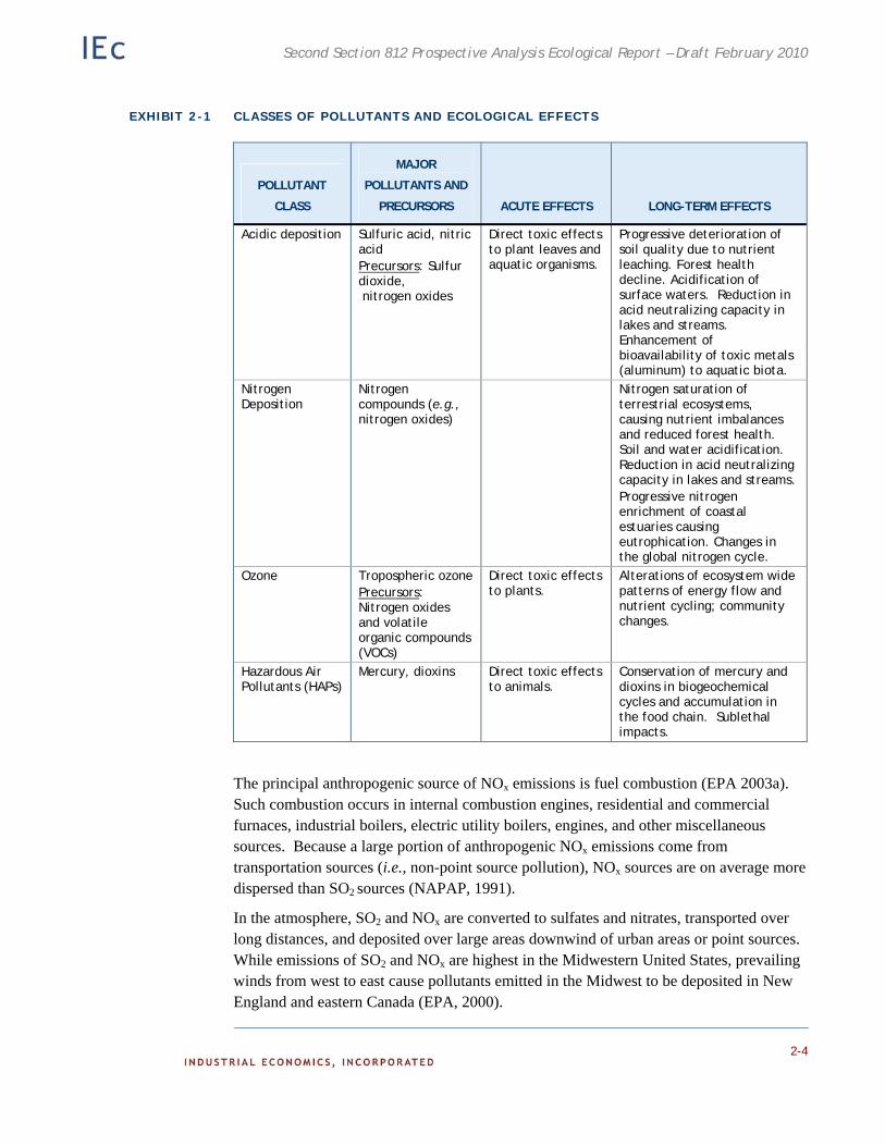


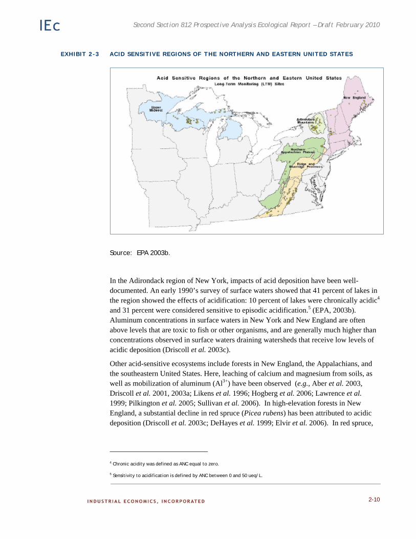


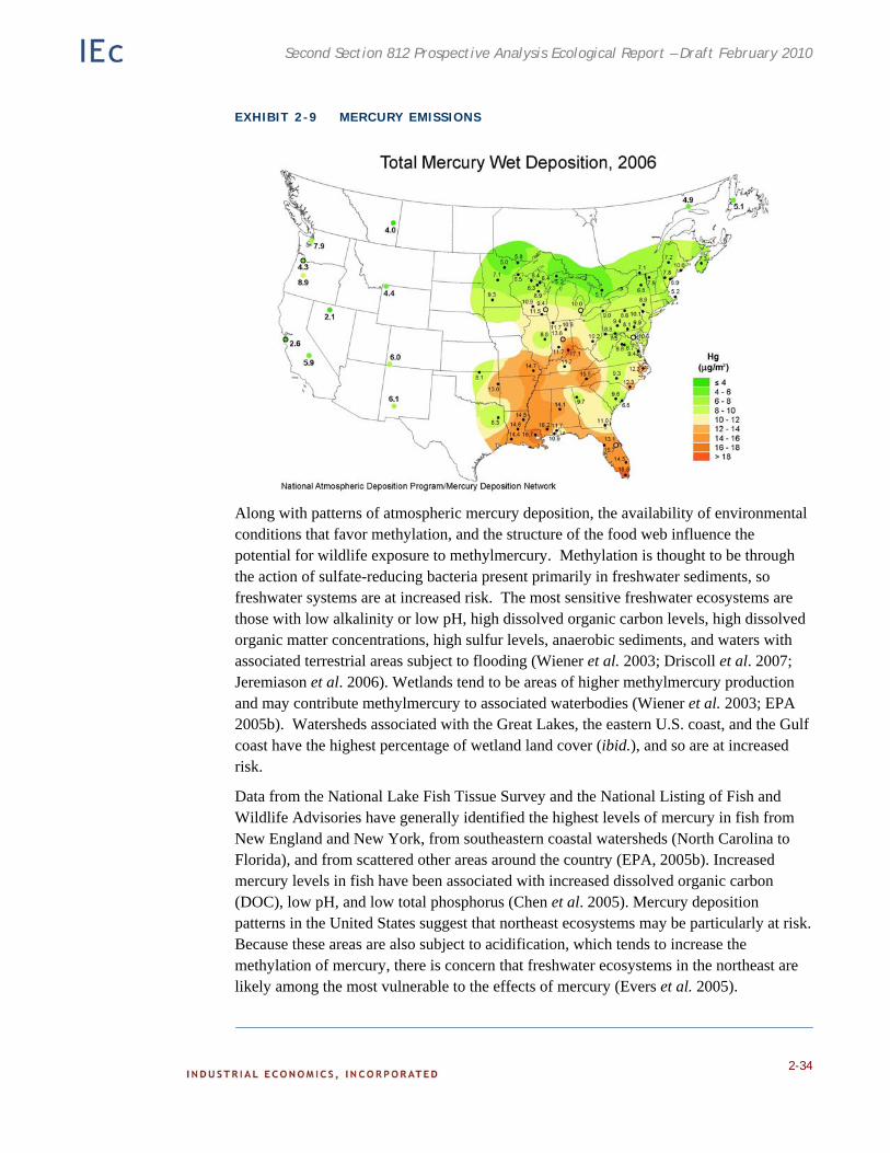


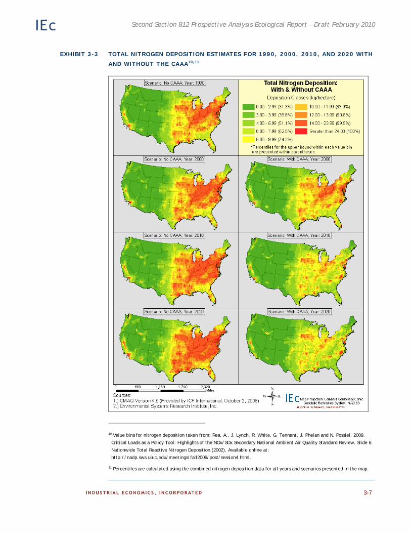


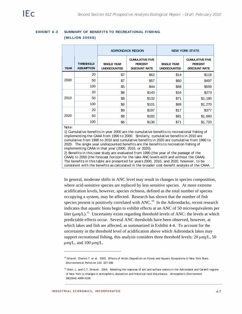

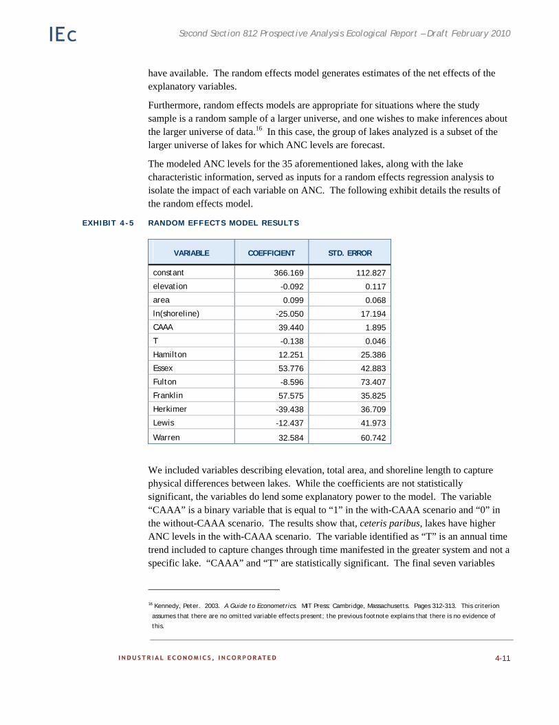


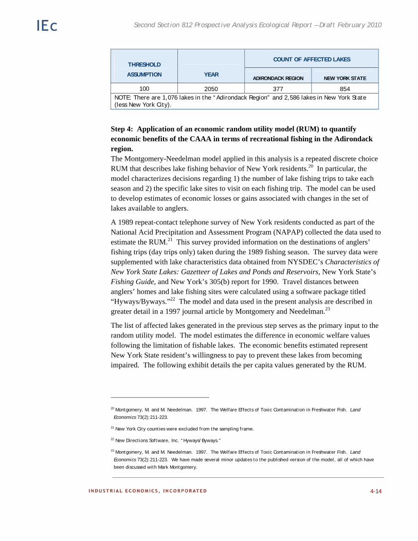
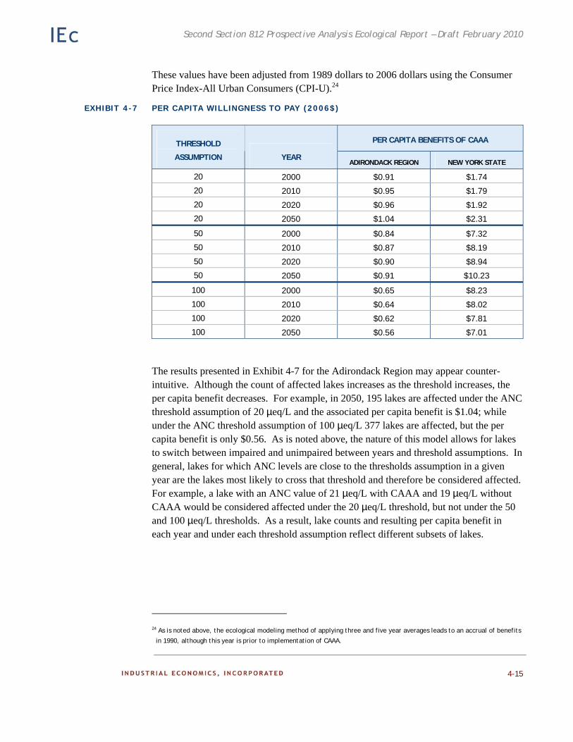

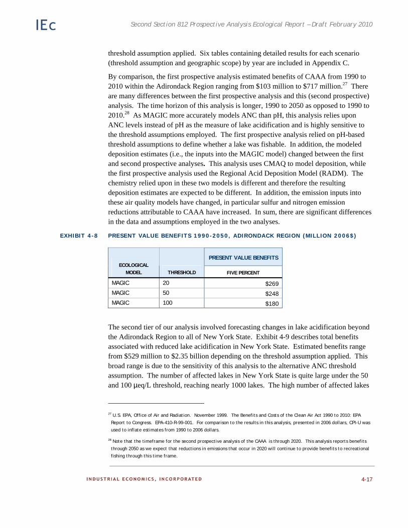
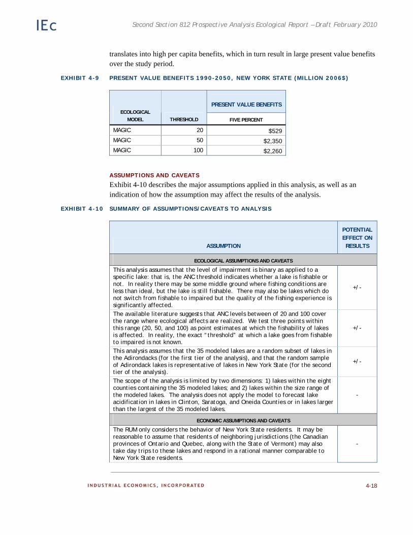


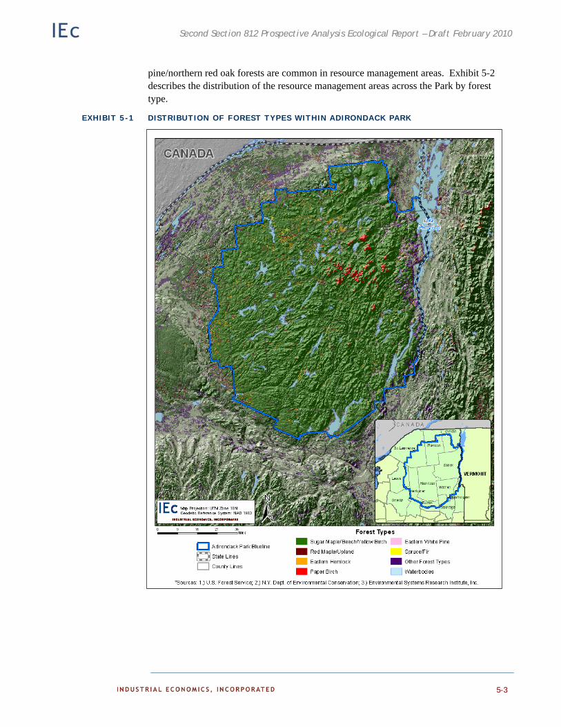
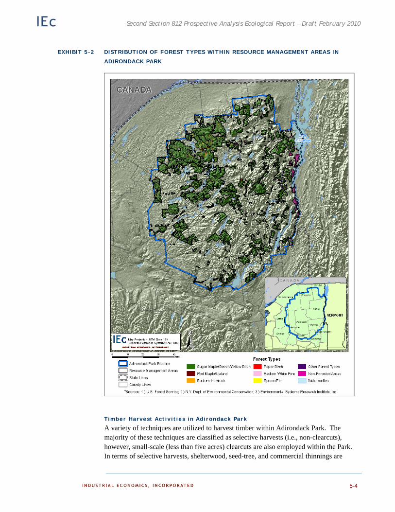


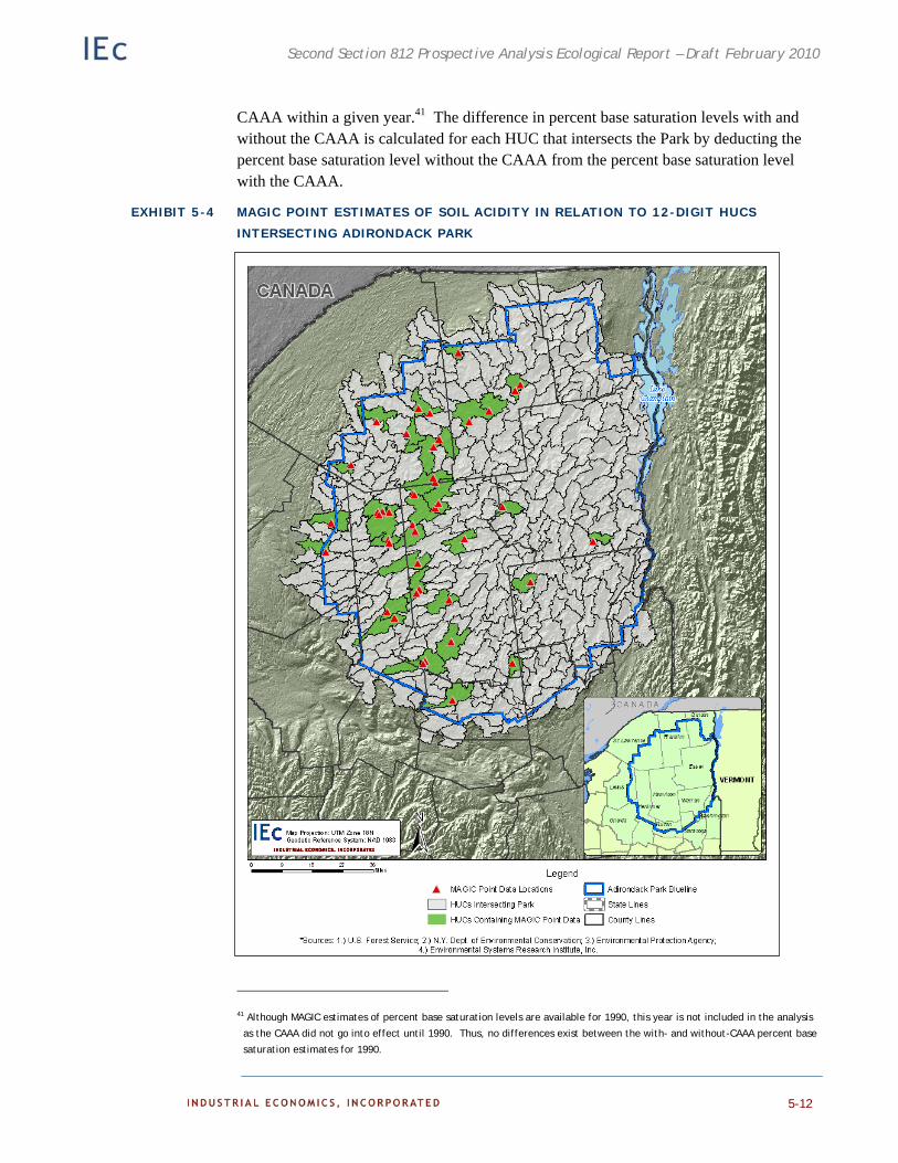

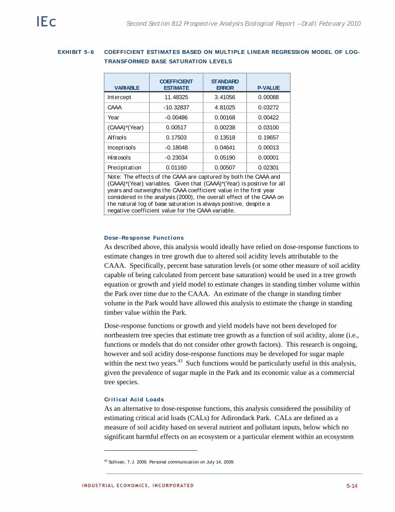


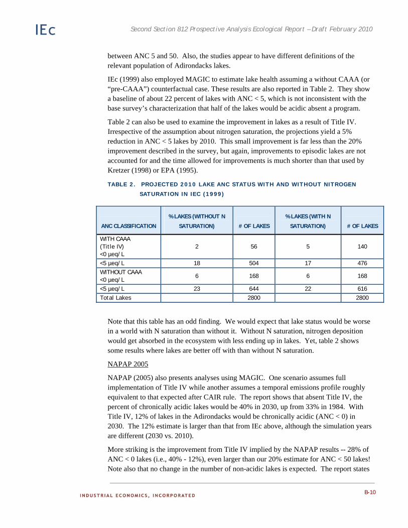
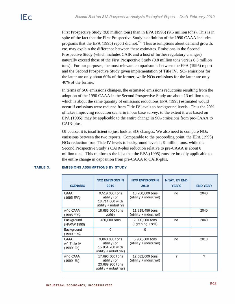


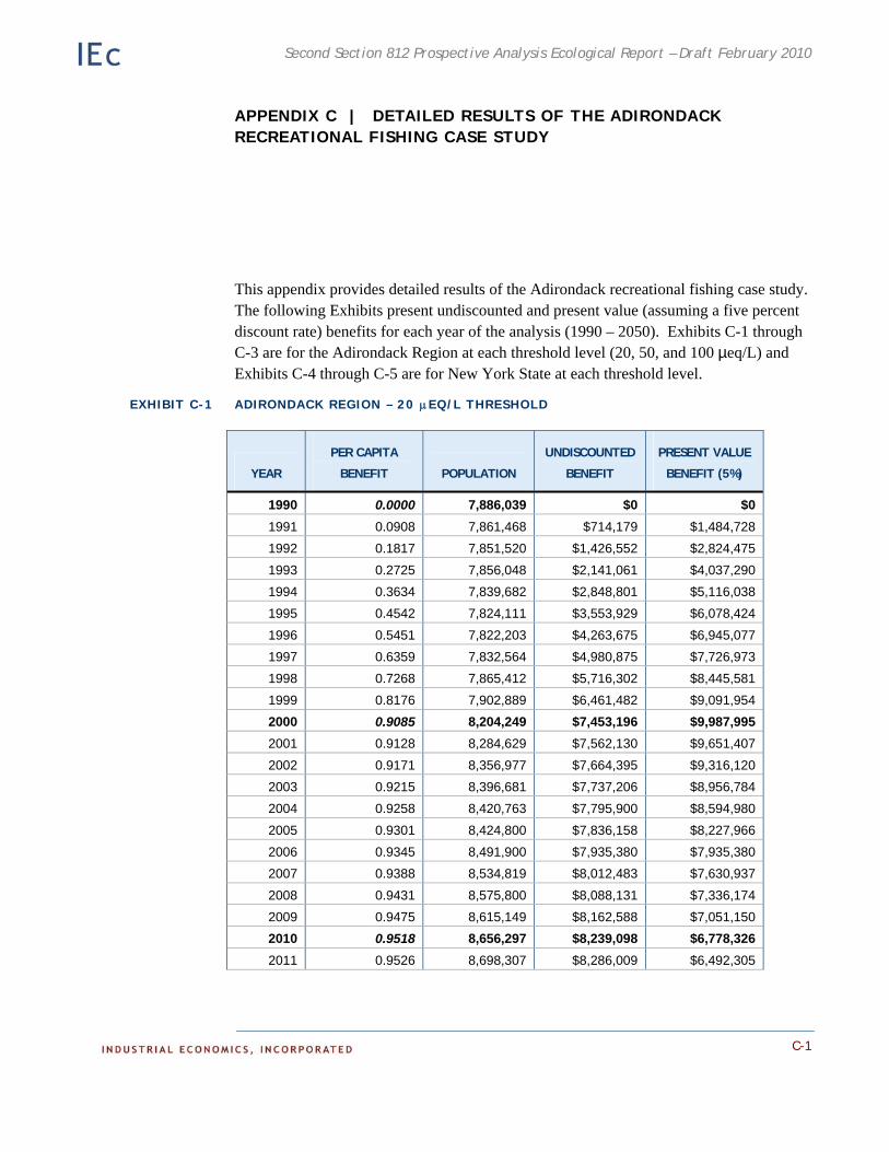

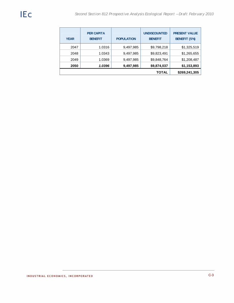
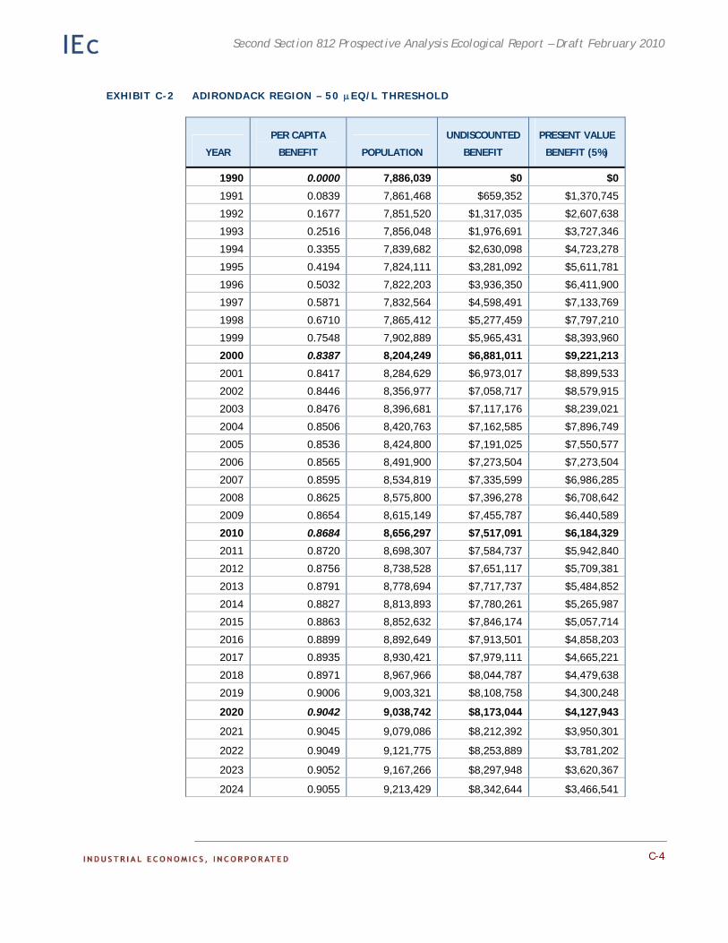
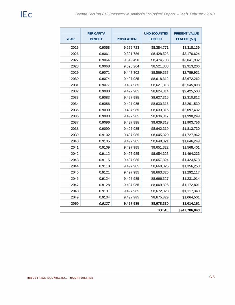
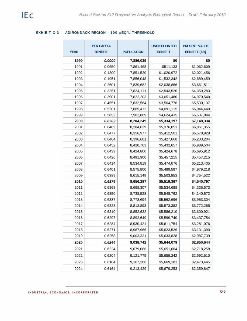

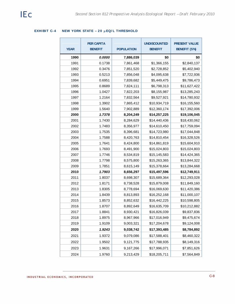


![D.6.1 [WP6 report] - feem-project.net part1 final.pdf · air pollutants and European average external cost of other pollutants, including costs of climate change. 1 Literature review](https://static.documents.pub/doc/80x56/5e447c683c54734118735f73/d61-wp6-report-feem-part1-finalpdf-air-pollutants-and-european-average.jpg)


