Walther et al. Vol. 25, No. 11 /November 2008 /J. Opt. Soc. Am. A 2791
Effects of axial, transverse, and oblique samplemotion in FD OCT in systems with global
or rolling shutter line detector
Julia Walther,1,* Alexander Krüger,2 Maximiliano Cuevas,1 and Edmund Koch1
1Department of Clinical Sensoring and Monitoring, Medical Faculty Carl Gustav Carus, University of TechnologyDresden, Fetscherstrasse 74, 01307 Dresden, Germany
2Department of Biophotonics and Laser Medicine, Laser Zentrum Hannover e.V., Hollerithallee 8,30419 Hannover, Germany
. INTRODUCTIONptical coherence tomography (OCT) is a high-resolution
maging technique for noninvasive, in vivo examinationsf subsurface tissue based on low-coherence interferom-try using near-infrared light [1,2]. Because of movementf investigated living tissue during data acquisition sig-ificant motion artifacts occur. By ignoring this sampleotion in image processing, image quality will be de-
raded and a precise medical opinion will be impeded.ifferent novel technologies in data acquisition have beeneveloped to reduce motion effects in OCT images [3–5].ut the modality and dimension of motion artifacts inonventional OCT images receive less attention in OCTesearch. Therefore, it is essential to analyze the effects ofxial, transverse, and oblique motion, and to understandhe decrease in signal power in OCT images.
Image artifacts caused by axial and transverse motionave been previously described for Fourier-domain (FD)CT systems with a spectrometer or swept source [6]. In
he case of the axially moving sample, a Doppler fre-uency shift depending on the ratio of frequency sweepate and axial velocity of the sample was observed for thewept-source system. This Doppler shift results in an er-oneous depth offset that is not present in the FD OCTystem using a spectrometer.
In this study, we show that the observation above ap-lies only for spectrometers utilizing line detectors with alobal shutter. In spectrometers containing line detectorsith a rolling shutter, a Doppler shift occurs that has a
imilar distortion effect on the axial position measure-ent of moving objects as described for swept-source sys-
ems. Furthermore, we compare both systems with differ-nt detectors in consideration of pure transverse andblique sample motion. We show that the effect of obliqueotion is not simply the sum of transverse and axial mo-
ion. In addition, the possibility of measuring flow by us-ng signal power decrease is shown by a flow phantom
odel.
. FOURIER-DOMAIN OPTICAL COHERENCEOMOGRAPHYD OCT, which is based on the spectral analysis of the in-
erference signal, is gaining considerable interest due tots high sensitivity and image acquisition speed comparedith time-domain OCT (TD OCT). Two different systemsased on FD OCT are found in the literature—one using apectrometer (spectral domain OCT, SD OCT) [7–10] andhe other using a frequency-swept light source (opticalrequency-domain imaging, OFDI) [11–13]. In SD OCT,he interference signal is analyzed in the spatial domain.n contrast, OFDI measures the interference signal as aunction of time.
. System Setuphe two investigated FD OCT systems are based on SDCT and consist of a broadband short coherent light
ource (SLD, � =840 nm, FWHM=50 nm, Superlum),
center
008 Optical Society of America
asilatsddftOpdbItfi3r
u(ruTepsrl1g0dsc
BTdrgs
w
S
�xr
g
xz
tT
3AAsTzBtn
Tt�iew
msttmc
Fss
2792 J. Opt. Soc. Am. A/Vol. 25, No. 11 /November 2008 Walther et al.
2D or 3D scanner, and a fiber-coupled spectrometer, ashown in Fig. 1. The modified Michelson interferometer isntegrated in the scanner head, where the broadbandight of the SLD is split into a sample and a referencerm. The backscattered light from within the sample andhe reference light are superimposed and directed to thepectrometer, consisting of a diffraction grating and a lineetector. This spectrum is rescaled to wavenumber k. Theepth profile (A-scan) is determined by a Fourier trans-ormation of the spectral interference pattern recorded byhe line detector of the spectrometer [7]. To obtain a 2DCT image (B-scan) or a 3D OCT volume scan, a multi-licity of A-scans must be acquired. This is achieved byeflecting the sample beam along a transverse directiony two galvanometer scanners (Cambridge Technology,nc.). By using the 2D scanner, the sample beam has aheoretically calculated FWHM of the beam intensity pro-le of w0=5.83 �m. Because of the different optics of theD scanner head compared to the 2D scanner, the theo-etical FWHM w0 is 7.3 �m.
Our two FD OCT systems differ in the type of detectortilized. System A uses the line detector Dalsa IL-C6DALSA) with a global shutter, while system B has theolling shutter detector LIS-1024 (Panavision), which issed in commercially available instruments, too (Fig. 1).he difference between the detectors is that the start andnd points of the integration period are different for eachixel of a detector with a rolling shutter, in contrast to aystem with a global shutter, where the integration pe-iod is identical for each pixel [14–16]. The global shutterine detector of system A can operate at a readout rate of.2 kHz to 11.88 kHz with a duty cycle of 100%. The inte-ration time of the rolling shutter line detector TA-scan is.84 ms and corresponds to a readout rate of 1.2 kHz. Theuty cycle of system B is �99%. The depth range of bothystems is approximately 2 mm. Both systems are appli-able with the 2D or 3D scanner.
. Interference Signalhe equation that describes the photocurrent has beenerived in detail by S. H. Yun et al. [6]. Briefly summa-ized, the photocurrent reflects the interference fringesenerated by the superposition of the reference and theample light and can be expressed as
ig. 1. Principle of the FD OCT with spectrometer and the 3Dcanner head, as well as the data processing is shown. (I, inten-ity; FFT, fast Fourier transformation; z, depth)
i�k� = c Re�� �� r�x,y,z�g�x − xb,y − yb,z − zb�
�exp�− i2k�z − zb��dxdydz� , �1�
ith c=��Sr�k�Ss�k�.Terms and variables are as follows:
r�k�, Ss�k� spectral power density of the reference andsample armspectrometer and quantum efficiency
,y ,z coordinates of the reference fixed to the sample�x ,y ,z� complex-valued backscattering coefficient of
the sample�x ,y ,z� intensity profile of the sample beam including
the detection sensitivity normalized togdxdy=1
b, yb transverse coordinates of the sample beamb longitudinal coordinate of the zero path length
point of the interferometer
The number of electrons N�k� can be calculated by in-egrating the photocurrent over the integration timeA-scan [6]:
N�k� = c Re��−TA-scan/2
TA-scan/2 ��� r�x,y,z�g�x − xb,y − yb�
�exp�− i2k�z − zb��dxdydzdt� . �2�
. EFFECTS OF AXIAL MOTION. Theoryxial motion can be described by the change of the z po-ition of the sample relative to the scanner head duringA-scan. Therefore, zb in Eq. (2) must be replaced by
b−vzt, where vz corresponds to the axial sample velocity.y performing the time integration, it can be seen that
he axial motion leads to an attenuation of the signal-to-oise ratio (SNR) by a factor � [6].
SNR��z� = SNR��z = 0�� � =sin2�k0�z�
�k0�z�2 , � = �0,1�.
�3�
he variable �z denotes the axial displacement ofhe sample during TA-scan and can be described byz=vzTA-scan. The center wavenumber of the light source
s indicated by k0. Because of the large confocal param-ter, the change in beam diameter due to axial motionas neglected.Rolling shutter line detector. Because of the time do-ain character of the SD OCT system using a rolling
hutter line detector, similar motion artifacts compared tohe system based on OFDI are expected. In OFDI sys-ems, a Doppler frequency shift is added to the originalodulation frequency of the interference signal [6] and
an be described by
wDpT
BTfsAoisr7wawm
COAAFAi5titdA
wwalz(tt
m(dwrtl
FA(�ss
Fs(s
FAAst
Walther et al. Vol. 25, No. 11 /November 2008 /J. Opt. Soc. Am. A 2793
z�t� = z0�t� + zD, �4�
zD =k0
�k�z, �5�
here z0�t� denotes the sample movement and zD is theoppler axial shift in the OCT images. Note that zD de-ends on the time t via vz but also on the integration timeA-scan.
. Experimentso realize axial sample motion, we attached a rough goldoil to a loudspeaker. In this experiment the galvanometercanner in the scanner head remained still. This way all-scans have an identical xy position. The axial position zf the gold foil at zero voltage applied to the speaker co-ncides with the focal plane of the imaging lens. Thepeaker was driven with a sinusoidal voltage waveformesulting in a peak-to-peak mechanical amplitude App of0 �m at frequencies fLS ranging from 5 to 100 Hz. Appas controlled by a fast triangulation sensor and showeddeviation less than ±5%. M-mode images were acquiredith both OCT systems for analyzing the time resolvedotion of the speaker at different frequencies fLS.
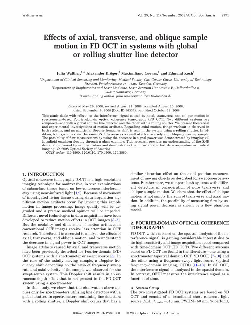
. ResultsCT M-mode images consisting of a time series of 1008-scans (total 0.84 s) were acquired with system A at an-scan frequency fA-scan of 1.2 kHz and the 2D scanner.igure 2 shows only 500 A-scans of the 1008 acquired-scans. The vertical axis consists of 77 pixels represent-
ng a depth of 0.36 mm. At a speaker frequency fLS ofHz, there are noticable points of fringe washout (arrows
op left) and different intensities depending on the veloc-ty of the gold foil. Fringe washout is caused by the con-inuous phase change of the interference pattern on theetector due to speaker movement of � /2 during an-scan. The maximum intensity (arrows top right) occurs
ig. 2. (Color online) M-mode images (only 500 of a total of 1008-scans) of the gold foil fixed on the sinusoidally moving speaker
fLS=5,10,50,100 Hz; App=70 �m) acquired with system AfA-scan=1.2 kHz� are shown. The framed parts on the right-handides of the two bottom rows show enlarged views of the corre-ponding areas on the left.
hen the velocity of the gold foil comes close to zeroithin TA-scan. With higher frequencies �10–100 Hz� themplitude stays constant, but because of the higher ve-ocities the fringe washout cannot be resolved. In theoom view of the M-mode images at fLS of 50 and 100 Hzframed parts), one can still see maximum intensities athe peaks of the sinusoidal movement and decreased in-ensities at the points of highest velocity.
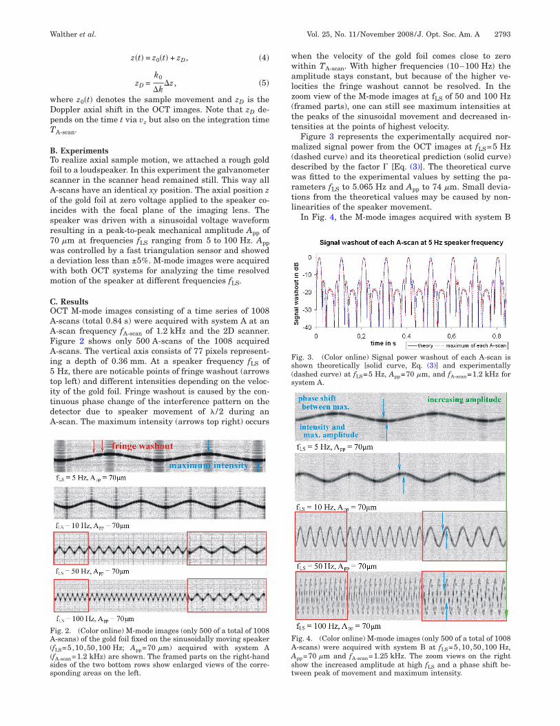
Figure 3 represents the experimentally acquired nor-alized signal power from the OCT images at fLS=5 Hz
dashed curve) and its theoretical prediction (solid curve)escribed by the factor � [Eq. (3)]. The theoretical curveas fitted to the experimental values by setting the pa-
ameters fLS to 5.065 Hz and App to 74 �m. Small devia-ions from the theoretical values may be caused by non-inearities of the speaker movement.
In Fig. 4, the M-mode images acquired with system B
ig. 3. (Color online) Signal power washout of each A-scan ishown theoretically [solid curve, Eq. (3)] and experimentallydashed curve) at fLS=5 Hz, App=70 �m, and fA-scan=1.2 kHz forystem A.
ig. 4. (Color online) M-mode images (only 500 of a total of 1008-scans) were acquired with system B at fLS=5,10,50,100 Hz,pp=70 �m and fA-scan=1.25 kHz. The zoom views on the righthow the increased amplitude at high fLS and a phase shift be-ween peak of movement and maximum intensity.
aTptatfspvds
toaOatiovm
DTisgisplsbtqwa=
s=mOt
4ABs(
w
EoitcTbs
w
wldsts
BJwtprmmrmrttcdtrr
Fa
2794 J. Opt. Soc. Am. A/Vol. 25, No. 11 /November 2008 Walther et al.
t fA-scan=1.25 kHz and the 2D scanner are presented.he vertical axis consists of 138 pixels. In addition to theoints of total fringe washout, an increase of the ampli-ude with rising speaker frequency (arrow at right edge)nd an additional phase shift between maximum ampli-ude and maximum intensity (arrows nearly facing in allour rows) are observed. This is in contrast to the datahown in Fig. 2. The reason for these effects is the Dop-ler frequency shift zD described by Eqs. (4) and (5). Theariable � denotes the factor of amplitude increase and isescribed by Eq. (6). The occurring phase shift is pre-ented in Eq. (7):
� =z�t�
z0�t�=�1 + � k0
�k�LSTA-scan�2
, �6�
= arctan� k0
�k�LSTA-scan� . �7�
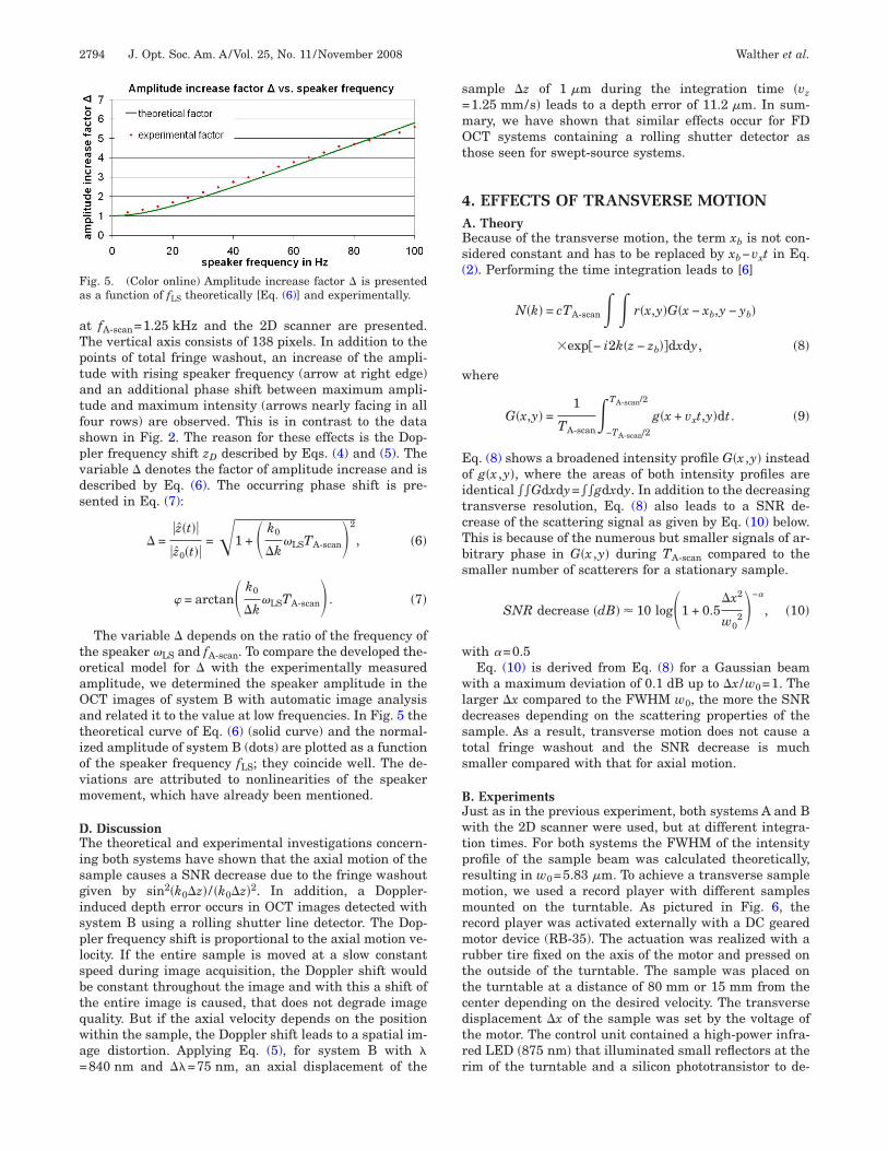
The variable � depends on the ratio of the frequency ofhe speaker �LS and fA-scan. To compare the developed the-retical model for � with the experimentally measuredmplitude, we determined the speaker amplitude in theCT images of system B with automatic image analysisnd related it to the value at low frequencies. In Fig. 5 theheoretical curve of Eq. (6) (solid curve) and the normal-zed amplitude of system B (dots) are plotted as a functionf the speaker frequency fLS; they coincide well. The de-iations are attributed to nonlinearities of the speakerovement, which have already been mentioned.
. Discussionhe theoretical and experimental investigations concern-
ng both systems have shown that the axial motion of theample causes a SNR decrease due to the fringe washoutiven by sin2�k0�z� / �k0�z�2. In addition, a Doppler-nduced depth error occurs in OCT images detected withystem B using a rolling shutter line detector. The Dop-ler frequency shift is proportional to the axial motion ve-ocity. If the entire sample is moved at a slow constantpeed during image acquisition, the Doppler shift woulde constant throughout the image and with this a shift ofhe entire image is caused, that does not degrade imageuality. But if the axial velocity depends on the positionithin the sample, the Doppler shift leads to a spatial im-ge distortion. Applying Eq. (5), for system B with �840 nm and ��=75 nm, an axial displacement of the
ig. 5. (Color online) Amplitude increase factor � is presenteds a function of fLS theoretically [Eq. (6)] and experimentally.
ample �z of 1 �m during the integration time �vz1.25 mm/s� leads to a depth error of 11.2 �m. In sum-ary, we have shown that similar effects occur for FDCT systems containing a rolling shutter detector as
hose seen for swept-source systems.
. EFFECTS OF TRANSVERSE MOTION. Theoryecause of the transverse motion, the term xb is not con-idered constant and has to be replaced by xb−vxt in Eq.2). Performing the time integration leads to [6]
N�k� = cTA-scan�� r�x,y�G�x − xb,y − yb�
�exp�− i2k�z − zb��dxdy, �8�
here
G�x,y� =1
TA-scan�
−TA-scan/2
TA-scan/2
g�x + vxt,y�dt. �9�
q. (8) shows a broadened intensity profile G�x ,y� insteadf g�x ,y�, where the areas of both intensity profiles aredentical Gdxdy=gdxdy. In addition to the decreasingransverse resolution, Eq. (8) also leads to a SNR de-rease of the scattering signal as given by Eq. (10) below.his is because of the numerous but smaller signals of ar-itrary phase in G�x ,y� during TA-scan compared to themaller number of scatterers for a stationary sample.
SNR decrease �dB� 10 log�1 + 0.5�x2
w02�−
, �10�
ith =0.5Eq. (10) is derived from Eq. (8) for a Gaussian beam
ith a maximum deviation of 0.1 dB up to �x /w0=1. Thearger �x compared to the FWHM w0, the more the SNRecreases depending on the scattering properties of theample. As a result, transverse motion does not cause aotal fringe washout and the SNR decrease is muchmaller compared with that for axial motion.
. Experimentsust as in the previous experiment, both systems A and Bith the 2D scanner were used, but at different integra-
ion times. For both systems the FWHM of the intensityrofile of the sample beam was calculated theoretically,esulting in w0=5.83 �m. To achieve a transverse sampleotion, we used a record player with different samplesounted on the turntable. As pictured in Fig. 6, the
ecord player was activated externally with a DC gearedotor device (RB-35). The actuation was realized with a
ubber tire fixed on the axis of the motor and pressed onhe outside of the turntable. The sample was placed onhe turntable at a distance of 80 mm or 15 mm from theenter depending on the desired velocity. The transverseisplacement �x of the sample was set by the voltage ofhe motor. The control unit contained a high-power infra-ed LED �875 nm� that illuminated small reflectors at theim of the turntable and a silicon phototransistor to de-
tfl
AstsslAt
spatf2rIe
CFasMt1ersr
tMFctosfo
4waTbtm
csfv0scsiv
Fv2mr
FmsSm
Walther et al. Vol. 25, No. 11 /November 2008 /J. Opt. Soc. Am. A 2795
ect the reflected light. The frequency of the “running” re-ectors was controlled by an oscilloscope.The galvanometer scanner remained still, so that all
-scans were detected with an identical xy position of theample beam. To start data acquisition, a gold foil fixed athe same distance from the turntable center as theample was used. This trigger unit guaranteed that theame area of the sample is detected regardless of the ve-ocity vx. For each measurement, the same number of-scans was acquired, which meant that for higher veloci-
ies vx, the sample passed by the sample beam repeatedly.To examine the SNR decrease, four different types of
amples were used: aluminium foil (matt finished), whiteaper, 20% Intralipid emulsion (SMOFlipid, Fresenius),nd the frosted stripe of a microscope slide (Elka, Assis-ant). We expected that the aluminium foil and therosted surface of the microscope slide would behave likeD scattering layers with scattering processes at theough surface. In contrast to this, white paper and 20%ntralipid emulsion were assumed to be volume homog-nous random scattering samples.
. Resultsigure 7 shows the M-mode images of three sample typest the normalized displacement �x /w0=1.5, which corre-ponds to a transverse velocity of vx=104 mm/s. These-mode images consist of 795 A-scans acquired with sys-
em A at fA-scan of 11.88 kHz. The vertical axis consists of59 pixels representing a depth of 0.75 mm. Note that thentire measurement consists of 11 passes of the sampleelative to the sample beam. Furthermore, Fig. 7(a)hows that there are small variations in z position fromound to round.
To ascertain the SNR drop with increasing velocity vx,he signal peak power (in dB) of each A-scan of one-scan is determined and averaged over all 795 A-scans.or the aluminium sample, the signal peak power is as-ertained in a definite region of interest (ROI) marked byhe two horizontal dashed lines [Fig. 7(a)]. In contrast,nly one pixel designated by the single dashed line is ob-erved for the volume scatterers. The experiment is per-ormed for normalized displacements �x /w0 in the rangef 0.3 and 6, which correspond to velocities v of 21 and
ig. 6. (Color online) Setup for the measurements of a trans-ersely moved sample, e.g., a microscope slide, is presented. TheD scanner head is positioned orthogonally to the sampleounted on the turntable, which is activated externally with a
ubber tire fixed on the axis of the motor.
x
15 mm/s, respectively. The fitting according to Eq. (10),here the exponent and the value at zero were the onlyrbitrary parameters, is plotted as a solid curve in Fig. 7.he aluminium foil behaves like a 2D random scattererecause =0.5. The determined value of the paper andhe Intralipid sample is almost 0.5, as expected for a ho-ogenous volume random scattering medium.The diagram in Fig. 8(a) shows the SNR decrease
aused by the transversely moving frosted microscopelide as a function of �x /w0 detected by system A at anA-scan of 1.49 kHz with the 2D scanner. The set velocitiesary between 0 and 71 mm/s and correspond to �x /w0 ofto 8.2 with w0 of 5.83 �m. For each velocity, two mea-
urements were carried out (dots). In contrast to the pre-eding measurements, the microscope slide passed theample beam only one time, so that the number of A-scansn the M-mode image decreases with increasing velocity
. As expected, the microscope slide behaves like a 2D
ig. 7. (Color online) SNR decrease (in dB) due to transverseotion is measured as a function of �x /w0. The solid curve con-
ists two superimposed (or nearly so) curves, one for theoreticalNR drop and one for the fitting according to Eq. (10). (a) Alu-inium foil, =0.51, (b) paper, =0.48, (c) Intralipid emulsion,=0.48.
x
r(Srscdfitc
DTtnodsct
fltisrl
5TATstFs�tz
w
Eopntstit
tgst�dspl
FmFtw=
Fmovl
2796 J. Opt. Soc. Am. A/Vol. 25, No. 11 /November 2008 Walther et al.
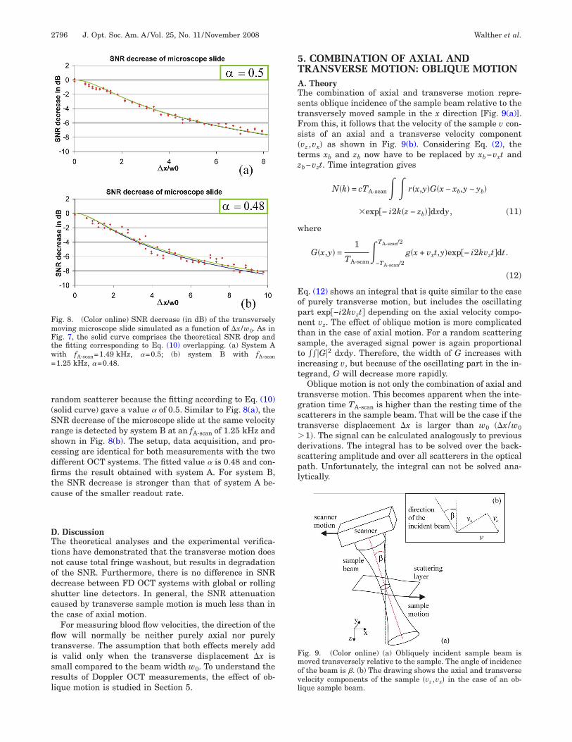
andom scatterer because the fitting according to Eq. (10)solid curve) gave a value of 0.5. Similar to Fig. 8(a), theNR decrease of the microscope slide at the same velocityange is detected by system B at an fA-scan of 1.25 kHz andhown in Fig. 8(b). The setup, data acquisition, and pro-essing are identical for both measurements with the twoifferent OCT systems. The fitted value is 0.48 and con-rms the result obtained with system A. For system B,he SNR decrease is stronger than that of system A be-ause of the smaller readout rate.
. Discussionhe theoretical analyses and the experimental verifica-ions have demonstrated that the transverse motion doesot cause total fringe washout, but results in degradationf the SNR. Furthermore, there is no difference in SNRecrease between FD OCT systems with global or rollinghutter line detectors. In general, the SNR attenuationaused by transverse sample motion is much less than inhe case of axial motion.
For measuring blood flow velocities, the direction of theow will normally be neither purely axial nor purelyransverse. The assumption that both effects merely adds valid only when the transverse displacement �x ismall compared to the beam width w0. To understand theesults of Doppler OCT measurements, the effect of ob-ique motion is studied in Section 5.
ig. 8. (Color online) SNR decrease (in dB) of the transverselyoving microscope slide simulated as a function of �x /w0. As inig. 7, the solid curve comprises the theoretical SNR drop andhe fitting corresponding to Eq. (10) overlapping. (a) System Aith fA-scan=1.49 kHz, =0.5; (b) system B with fA-scan1.25 kHz, =0.48.
. COMBINATION OF AXIAL ANDRANSVERSE MOTION: OBLIQUE MOTION. Theoryhe combination of axial and transverse motion repre-ents oblique incidence of the sample beam relative to theransversely moved sample in the x direction [Fig. 9(a)].rom this, it follows that the velocity of the sample v con-ists of an axial and a transverse velocity componentvz ,vx� as shown in Fig. 9(b). Considering Eq. (2), theerms xb and zb now have to be replaced by xb−vxt andb−vzt. Time integration gives
N�k� = cTA-scan�� r�x,y�G�x − xb,y − yb�
�exp�− i2k�z − zb��dxdy, �11�
here
G�x,y� =1
TA-scan�
−TA-scan/2
TA-scan/2
g�x + vxt,y�exp�− i2kvzt�dt.
�12�
q. (12) shows an integral that is quite similar to the casef purely transverse motion, but includes the oscillatingart exp�−i2kvzt� depending on the axial velocity compo-ent vz. The effect of oblique motion is more complicatedhan in the case of axial motion. For a random scatteringample, the averaged signal power is again proportionalo G2 dxdy. Therefore, the width of G increases withncreasing v, but because of the oscillating part in the in-egrand, G will decrease more rapidly.
Oblique motion is not only the combination of axial andransverse motion. This becomes apparent when the inte-ration time TA-scan is higher than the resting time of thecatterers in the sample beam. That will be the case if theransverse displacement �x is larger than w0 ��x /w01�. The signal can be calculated analogously to previous
erivations. The integral has to be solved over the back-cattering amplitude and over all scatterers in the opticalath. Unfortunately, the integral can not be solved ana-ytically.
ig. 9. (Color online) (a) Obliquely incident sample beam isoved transversely relative to the sample. The angle of incidence
f the beam is �. (b) The drawing shows the axial and transverseelocity components of the sample �vz ,vx� in the case of an ob-ique sample beam.
o2ldatscwtBaaitteptmtFtbttpw
cpbkcsto
tv1o
trocsn1
toctthahcA
BFvttptsf
Fs2lE
Ftlc1nt
Walther et al. Vol. 25, No. 11 /November 2008 /J. Opt. Soc. Am. A 2797
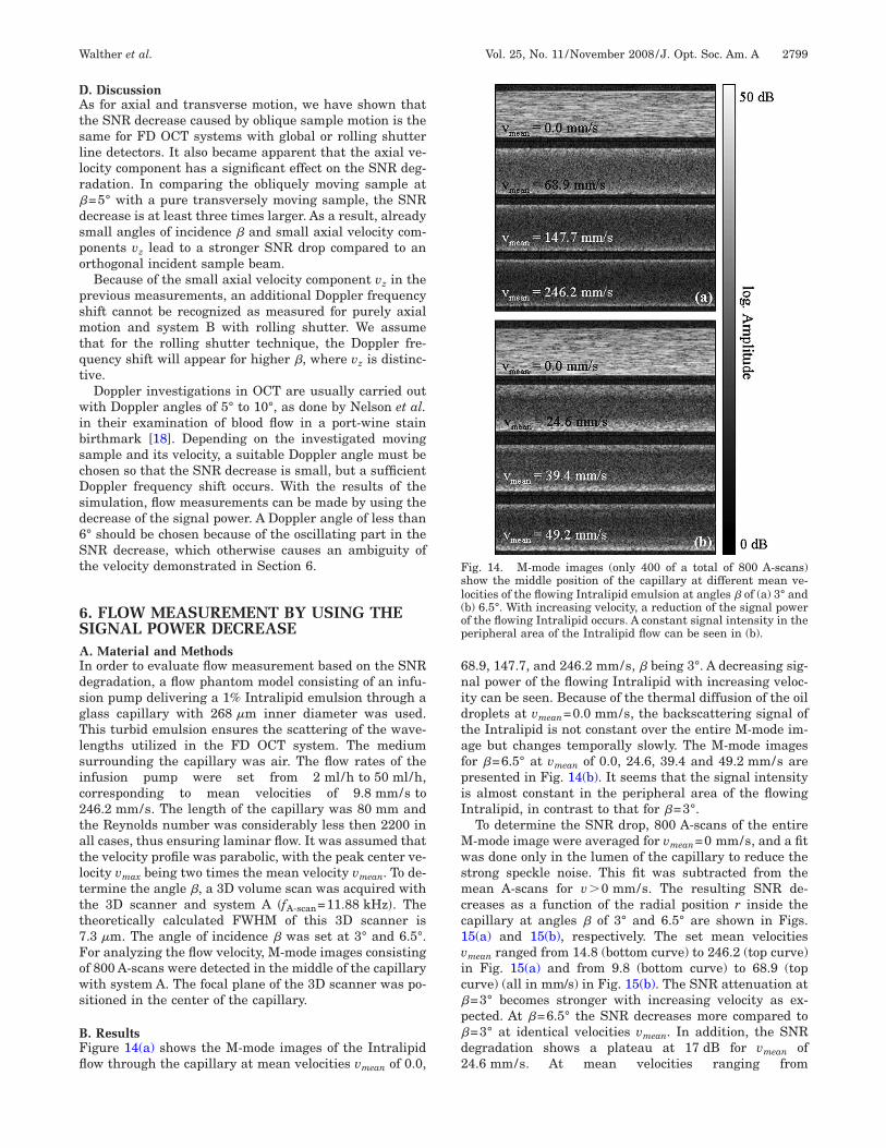
The simulation for system A with fA-scan of 1.49 kHz hasffered the signal decrease for angle � ranging from 0° to0° as shown in Fig. 10. Apparently, the effect of the ob-ique motion is not just the sum of the SNR decrease (inB) caused by transverse and axial motion [see Eqs. (11)nd (12)]. Therefore, in contrast to the purely axial mo-ion, no points of total fringe washout occur. But the re-ult shows that oscillations are present in the SNR de-rease. One would expect that these oscillations appearhen the axial component of the velocity �z is � /2 during
he integration time TA-scan irrespective of the set angle �.ut as shown by the simulated curves in Fig. 10, therere oscillations in the SNR decrease depending on the setngle �. The oscillations appear if the axial displacements at least � /2 within the beam diameter w0. Therefore,he critical angle is �crit�arcsin�� / �2w0�� where oscilla-ions occur in the SNR decrease. The reason for this un-xpected effect is that the scattering particles are notresent in the sample beam during the entire integrationime, which induces a reduced effective axial displace-ent �z. Consequently, the critical angle � depends on
he FWHM of the sample beam w0 as described before.urthermore, the Gaussian profile of the sample beam at-enuates the oscillations much more strongly than theoxcar window of the CCD detector. In addition, we notehat for transverse displacements �x larger than twicehe beam diameter vxTA-scan�2w0 the oscillations disap-ear. For small angles where v vx this means that thereill be no oscillations at v�2w0fA-scan.Because of the oscillating component in the SNR de-
rease, an ambiguity of the velocity occurs. Concerningure axial sample movement, the uniqueness limit woulde up to �z�� /2. In the case of oblique motion withnown angle �, the limit for disambiguity would still in-lude the range �z�� /2. As we have shown for anglesmaller than 6°, there is a monotonic SNR drop, so forhis case the uniqueness limit is limited only by the SNRf the signal.
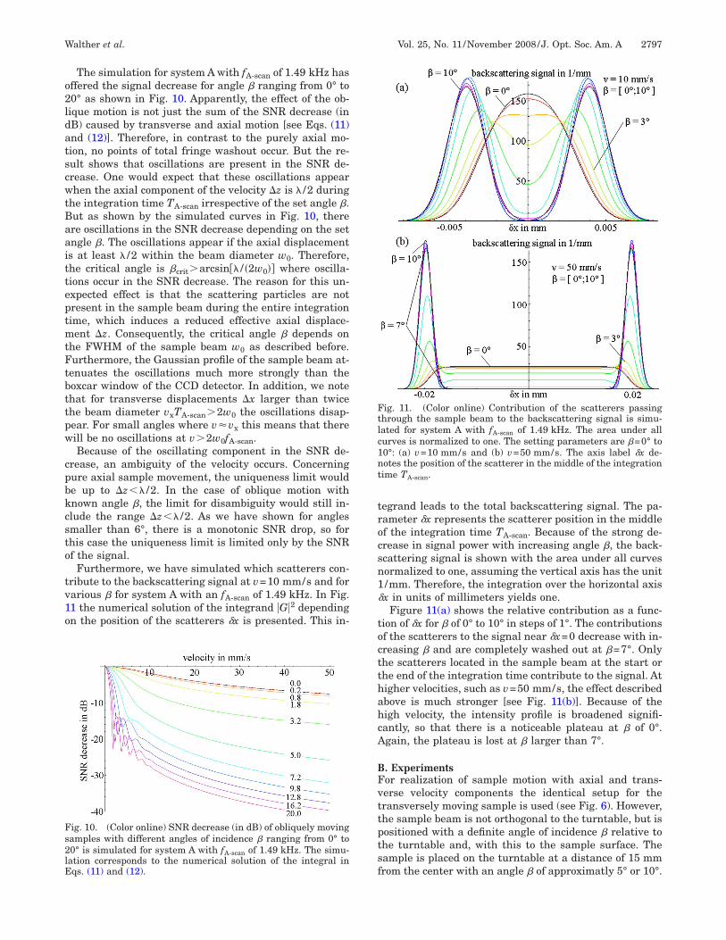
Furthermore, we have simulated which scatterers con-ribute to the backscattering signal at v=10 mm/s and forarious � for system A with an fA-scan of 1.49 kHz. In Fig.1 the numerical solution of the integrand G2 dependingn the position of the scatterers x is presented. This in-
ig. 10. (Color online) SNR decrease (in dB) of obliquely movingamples with different angles of incidence � ranging from 0° to0° is simulated for system A with fA-scan of 1.49 kHz. The simu-ation corresponds to the numerical solution of the integral inqs. (11) and (12).
egrand leads to the total backscattering signal. The pa-ameter x represents the scatterer position in the middlef the integration time TA-scan. Because of the strong de-rease in signal power with increasing angle �, the back-cattering signal is shown with the area under all curvesormalized to one, assuming the vertical axis has the unit/mm. Therefore, the integration over the horizontal axisx in units of millimeters yields one.
Figure 11(a) shows the relative contribution as a func-ion of x for � of 0° to 10° in steps of 1°. The contributionsf the scatterers to the signal near x=0 decrease with in-reasing � and are completely washed out at �=7°. Onlyhe scatterers located in the sample beam at the start orhe end of the integration time contribute to the signal. Atigher velocities, such as v=50 mm/s, the effect describedbove is much stronger [see Fig. 11(b)]. Because of theigh velocity, the intensity profile is broadened signifi-antly, so that there is a noticeable plateau at � of 0°.gain, the plateau is lost at � larger than 7°.
. Experimentsor realization of sample motion with axial and trans-erse velocity components the identical setup for theransversely moving sample is used (see Fig. 6). However,he sample beam is not orthogonal to the turntable, but isositioned with a definite angle of incidence � relative tohe turntable and, with this to the sample surface. Theample is placed on the turntable at a distance of 15 mmrom the center with an angle � of approximatly 5° or 10°.
ig. 11. (Color online) Contribution of the scatterers passinghrough the sample beam to the backscattering signal is simu-ated for system A with fA-scan of 1.49 kHz. The area under allurves is normalized to one. The setting parameters are �=0° to0°: (a) v=10 mm/s and (b) v=50 mm/s. The axis label x de-otes the position of the scatterer in the middle of the integrationime TA-scan.
Astmbis2
CTotBaneAaosmmt
t(vwcsabwtan
fAlcwTsImtfsi
btcsalnsspmfic
FlffSia(ssaog
Fstst�
2798 J. Opt. Soc. Am. A/Vol. 25, No. 11 /November 2008 Walther et al.
s a trigger for the start point of the data acquisition, themall piece of gold foil is used again and is oriented or-hogonal to the oblique incident sample beam. For theeasurement of the microscope slide, the sample passed
y the sample beam only once for the data acquisition. Asn the case of pure axially and transversely movedamples, we compared both systems A and B and used theD scanner.
. Resultshe diagrams in Fig. 12 show the SNR drop caused by thebliquely moved frosted microscope slide with �=5° de-ected by system A at an fA-scan of 1.49 kHz and by system
at an fA-scan of 1.25 kHz. The velocities vary between 0nd 50 mm/s. As with the previous measurement, a defi-ite ROI is selected in which the signal peak power ofach A-scan is ascertained and averaged over all acquired-scans. For each velocity, three measurements are aver-ged (Fig. 12, dots). The simulation of the decreasing SNRf an obliquely moved sample with �=5° is shown in theolid curve through the dots and corresponds to the nu-erical solution of the integral in Eqs. (11) and (12). Theeasured SNR decrease is in good agreement with the
heoretical curves.
ig. 12. (Color online) SNR decrease (in dB) arising from the ob-iquely moving microscope slide with �=5° is presented as aunction of the velocity (dots). (a) The results for system A withA-scan=1.49 kHz are shown. The upper solid curve represents theNR decrease for transverse velocity component vx correspond-
ng to Eq. (10). The darker sinusoidal curve describes the SNRttenuation for axial velocity component vz corresponding to Eq.3). The sum of SNR decreases for axial and transverse motion ishown by the lighter sinusoidal curve. (b) The measurement re-ults for system B with fA-scan=1.25 kHz are demonstrated. In (a)nd (b) the curve through the dots stands for the simulated the-retical SNR drop corresponding to the numerically solved inte-ral in Eqs. (11) and (12) with �=5°.
Additionally, Fig. 12(a) presents the SNR decrease forhe transverse component of the velocity vx=v cos���solid curve at top) and the axial velocity componentz=v sin��� (darker sinusoidal curve near the bottom), asell as the sum of both those curves (lighter sinusoidal
urve under the previous curve). The data shown mightuggest that the SNR drop for the oblique motion is justn interpolation of the maxima of the signal drop causedy the axial velocity component (darker sinusoidal curveith maxima close to the dots). In fact, for small angles,
he SNR penalty is much smaller, whereas for largerngles the drop might be greater than the sum of the sig-al drops caused by axial and transverse movement.SNR attenuation caused by the obliquely moving
rosted microscope slide with �=10.4° detected by systemat an fA-scan of 1.49 kHz is shown in Fig. 13. The simu-
ation for the decreasing SNR is represented in the solidurve. Compared to Fig. 12, an oscillating part is visible,hich is caused by the expression exp�−i2kvzt� in Eq. (12).he first cycle of oscillation in the simulated curve corre-ponds well with the measured values of the signal power.n contrast to this, the second cycle is hardly visible in theeasurement points because the standard deviation of
he three averaged measurements is too large for identi-ying the small oscillation of 0.5 dB. The remaining mea-urement points correspond well to the simulated theoret-cal curve.
Other sources for the deviations from the theory mighte a nonideal Gaussian beam profile and small oscilla-ions in the velocity of the turntable. The theoretical cal-ulations did not take the spectral range of the lightource into account, which can probably not be calculatednalytically in the case of a finite spectral range of theight source compared to the exponential term for the sig-al damping due to the spectral width of a Gaussianhaped light source given by H. Bachmann et al. [17]. Ashown in that previous study for purely axial motion, theolychromatic light results in a broadened signal thatay split up. But it is shown that this effect causes dif-
erences only at large spectral widths and when the signals strongly damped. Presumably this is also valid for thease of oblique motion.
ig. 13. (Color online) SNR decrease (in dB) of the microscopelide ��=10.4° � was measured as a function of the velocity de-ected by system A at fA-scan of 1.49 kHz. The solid curve repre-ents the simulated theoretical SNR decrease corresponding tohe numerical solution of the integral in Eqs. (11) and (12) with=10.4°.
DAtsllr�dspo
psmtqt
wibscDsd6St
6SAIdsgTlsic2tatlttt7Fows
BFfl
6nidtafpiI
Mwsmcc1vic�p�d2
Fsl(op
Walther et al. Vol. 25, No. 11 /November 2008 /J. Opt. Soc. Am. A 2799
. Discussions for axial and transverse motion, we have shown that
he SNR decrease caused by oblique sample motion is theame for FD OCT systems with global or rolling shutterine detectors. It also became apparent that the axial ve-ocity component has a significant effect on the SNR deg-adation. In comparing the obliquely moving sample at=5° with a pure transversely moving sample, the SNRecrease is at least three times larger. As a result, alreadymall angles of incidence � and small axial velocity com-onents vz lead to a stronger SNR drop compared to anrthogonal incident sample beam.
Because of the small axial velocity component vz in therevious measurements, an additional Doppler frequencyhift cannot be recognized as measured for purely axialotion and system B with rolling shutter. We assume
hat for the rolling shutter technique, the Doppler fre-uency shift will appear for higher �, where vz is distinc-ive.
Doppler investigations in OCT are usually carried outith Doppler angles of 5° to 10°, as done by Nelson et al.
n their examination of blood flow in a port-wine stainirthmark [18]. Depending on the investigated movingample and its velocity, a suitable Doppler angle must behosen so that the SNR decrease is small, but a sufficientoppler frequency shift occurs. With the results of the
imulation, flow measurements can be made by using theecrease of the signal power. A Doppler angle of less than° should be chosen because of the oscillating part in theNR decrease, which otherwise causes an ambiguity ofhe velocity demonstrated in Section 6.
. FLOW MEASUREMENT BY USING THEIGNAL POWER DECREASE. Material and Methods
n order to evaluate flow measurement based on the SNRegradation, a flow phantom model consisting of an infu-ion pump delivering a 1% Intralipid emulsion through alass capillary with 268 �m inner diameter was used.his turbid emulsion ensures the scattering of the wave-
engths utilized in the FD OCT system. The mediumurrounding the capillary was air. The flow rates of thenfusion pump were set from 2 ml/h to 50 ml/h,orresponding to mean velocities of 9.8 mm/s to46.2 mm/s. The length of the capillary was 80 mm andhe Reynolds number was considerably less then 2200 inll cases, thus ensuring laminar flow. It was assumed thathe velocity profile was parabolic, with the peak center ve-ocity vmax being two times the mean velocity vmean. To de-ermine the angle �, a 3D volume scan was acquired withhe 3D scanner and system A �fA-scan=11.88 kHz�. Theheoretically calculated FWHM of this 3D scanner is.3 �m. The angle of incidence � was set at 3° and 6.5°.or analyzing the flow velocity, M-mode images consistingf 800 A-scans were detected in the middle of the capillaryith system A. The focal plane of the 3D scanner was po-
itioned in the center of the capillary.
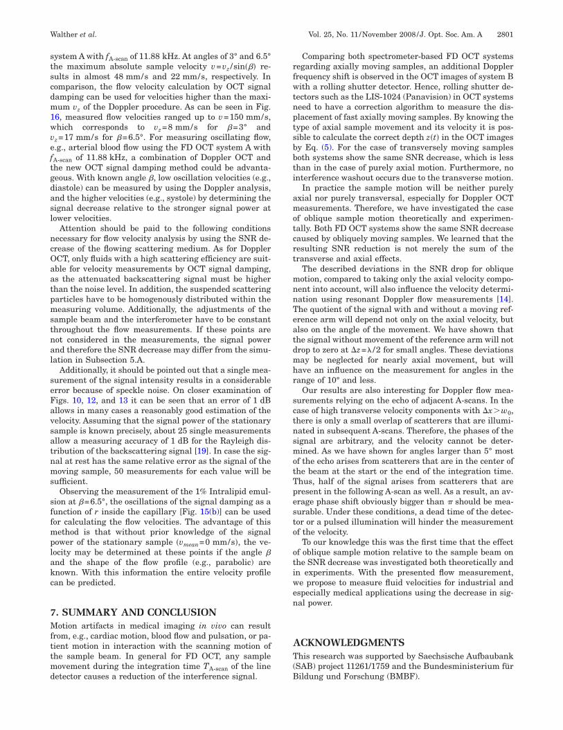
. Resultsigure 14(a) shows the M-mode images of the Intralipidow through the capillary at mean velocities v of 0.0,
mean
8.9, 147.7, and 246.2 mm/s, � being 3°. A decreasing sig-al power of the flowing Intralipid with increasing veloc-
ty can be seen. Because of the thermal diffusion of the oilroplets at vmean=0.0 mm/s, the backscattering signal ofhe Intralipid is not constant over the entire M-mode im-ge but changes temporally slowly. The M-mode imagesor �=6.5° at vmean of 0.0, 24.6, 39.4 and 49.2 mm/s areresented in Fig. 14(b). It seems that the signal intensitys almost constant in the peripheral area of the flowingntralipid, in contrast to that for �=3°.
To determine the SNR drop, 800 A-scans of the entire-mode image were averaged for vmean=0 mm/s, and a fitas done only in the lumen of the capillary to reduce the
trong speckle noise. This fit was subtracted from theean A-scans for v�0 mm/s. The resulting SNR de-
reases as a function of the radial position r inside theapillary at angles � of 3° and 6.5° are shown in Figs.5(a) and 15(b), respectively. The set mean velocitiesmean ranged from 14.8 (bottom curve) to 246.2 (top curve)n Fig. 15(a) and from 9.8 (bottom curve) to 68.9 (topurve) (all in mm/s) in Fig. 15(b). The SNR attenuation at=3° becomes stronger with increasing velocity as ex-ected. At �=6.5° the SNR decreases more compared to=3° at identical velocities vmean. In addition, the SNRegradation shows a plateau at 17 dB for vmean of4.6 mm/s. At mean velocities ranging from
ig. 14. M-mode images (only 400 of a total of 800 A-scans)how the middle position of the capillary at different mean ve-ocities of the flowing Intralipid emulsion at angles � of (a) 3° andb) 6.5°. With increasing velocity, a reduction of the signal powerf the flowing Intralipid occurs. A constant signal intensity in theeripheral area of the Intralipid flow can be seen in (b).
21ttnttflet=nelnpd
tHc=c−2shc
−utoTadcacvFtt
CTdsoTdpbBAt
Ftt1�oc
Ftlstwh
2800 J. Opt. Soc. Am. A/Vol. 25, No. 11 /November 2008 Walther et al.
9.5 to 34.5 mm/s the signal power decrease is less than7 dB. Furthermore, the SNR attenuation is almost iden-ical for r of −50 to 50 �m and independent of the set In-ralipid flow velocity. In this range the flow velocity can-ot be calculated because of an oscillating component inhe SNR attenuation at �=6.5°, as explained in Subsec-ion 5.A. This first oscillating part is also seen at higherow velocities and appears as small local maxima at thedges of the profile. On closer examination of Fig. 15(b),he local maxima at velocities higher than vmean34.5 mm/s have a SNR decrease less than 17 dB. This isot completely understood. We attribute it to the steepdge of the velocity profile compared to the axial reso-ution. At vmean of 49.2 mm/s a second plateau is recog-ized with a SNR drop of almost 20 dB, which can be ex-lained by a second cycle of oscillation in the velocity-ependent SNR decrease (see Subsection 5.A).The theoretical parabolic 2D velocity profile as a func-
ion of the radial position r can be calculated by usingagen–Poisseuille’s law. The SNR drop against these cal-
ulated velocities, both depending on r, is shown for �3° in Fig. 16(a) and for �=6.5° in Fig. 16(b). In bothases the entire SNR decrease for r ranging from134 to 134 �m is used for vmean between 14.8 and4.6 mm/s. Because of the poor axial resolution of theteep edges of the profiles and their small local maxima atigher velocities for vmean�29.5 mm/s, we take into ac-ount only the SNR decrease for r ranging from
ig. 15. (Color online) SNR decrease caused by the flowing In-ralipid is represented as a function of the radial position r insidehe glass capillary. The set mean velocities ranged from4.8 to 246.2 mm/s for �=3° (a) and from 9.8 to 68.9 mm/s for=6.5° (b). At �=6.5° [in (b)] plateaus in SNR decrease are rec-gnizable for vmean of 24.6 to 34.5 mm/s and vmean of 49.2 mm/sompared with �=3° [in (a)].
60 to 60 �m. In Figs. 16(a) and 16(b) the measured val-es conform well to the theoretical solid curve accordingo Eqs. (11) and (12) for w0 of 7.3 �m. The deviations thatccur are attributed to a depth-dependent SNR decrease.his becomes apparent especially at vmean�39.4 mm/snd �=3° because of different velocities at the same SNRecrease. The curve in Fig. 16(b) demonstrates a largeycle of oscillation followed by a small one, which leads tombiguity in calculating flow velocities from the SNR de-rease. We assume that deviations may also be caused byariations of the volume flow rate of the infusion pump.urthermore, our simulation considers only simple scat-
ering effects. Because of multiple-scattering processeshe SNR decrease may deviate from that expected.
. Discussionhe results of flow measurement using the signal powerecrease at the angles � of 3° and 6.5° presented in Sub-ections 6.A and 6.B are in good agreement with the the-retical examination and computation of Subsection 5.A.he advantage of flow measurement by using the signalecrease is that higher velocities can be evaluated com-ared to the established phase-resolved Doppler methody using the same spectrometer-based FD OCT system.y analysing the phase differences between adjacent-scans via Doppler FD OCT without any unwrapping
echniques, the maximum axial velocity v is 2.5 mm/s for
ig. 16. (Color online) SNR attenuation of the Intralipid flowinghrough the capillary is shown against the theoretically calcu-ated velocity for (a) �=3° and (b) �=6.5°. The solid curve repre-ents the simulated theoretical SNR decrease corresponding tohe numerical solution of the integral in Eqs. (11) and (12) for
0=7.3 �m. In (b) two cycles of oscillation are seen because of theigher axial velocity component compared with (a).
z
stscdm1wveftgdasl
ncOaatpmstnal
seFavsatnms
sffmplakc
7Mfttmd
rfwtnptsbbti
amotcrt
mnnTeatdmhr
sctnsmotTpesto
otiwen
AT(B
Walther et al. Vol. 25, No. 11 /November 2008 /J. Opt. Soc. Am. A 2801
ystem A with fA-scan of 11.88 kHz. At angles of 3° and 6.5°he maximum absolute sample velocity v=vz /sin��� re-ults in almost 48 mm/s and 22 mm/s, respectively. Inomparison, the flow velocity calculation by OCT signalamping can be used for velocities higher than the maxi-um vz of the Doppler procedure. As can be seen in Fig.
6, measured flow velocities ranged up to v=150 mm/s,hich corresponds to vz=8 mm/s for �=3° and
z=17 mm/s for �=6.5°. For measuring oscillating flow,.g., arterial blood flow using the FD OCT system A withA-scan of 11.88 kHz, a combination of Doppler OCT andhe new OCT signal damping method could be advanta-eous. With known angle �, low oscillation velocities (e.g.,iastole) can be measured by using the Doppler analysis,nd the higher velocities (e.g., systole) by determining theignal decrease relative to the stronger signal power atower velocities.
Attention should be paid to the following conditionsecessary for flow velocity analysis by using the SNR de-rease of the flowing scattering medium. As for DopplerCT, only fluids with a high scattering efficiency are suit-ble for velocity measurements by OCT signal damping,s the attenuated backscattering signal must be higherhan the noise level. In addition, the suspended scatteringarticles have to be homogenously distributed within theeasuring volume. Additionally, the adjustments of the
ample beam and the interferometer have to be constanthroughout the flow measurements. If these points areot considered in the measurements, the signal powernd therefore the SNR decrease may differ from the simu-ation in Subsection 5.A.
Additionally, it should be pointed out that a single mea-urement of the signal intensity results in a considerablerror because of speckle noise. On closer examination ofigs. 10, 12, and 13 it can be seen that an error of 1 dBllows in many cases a reasonably good estimation of theelocity. Assuming that the signal power of the stationaryample is known precisely, about 25 single measurementsllow a measuring accuracy of 1 dB for the Rayleigh dis-ribution of the backscattering signal [19]. In case the sig-al at rest has the same relative error as the signal of theoving sample, 50 measurements for each value will be
ufficient.Observing the measurement of the 1% Intralipid emul-
ion at �=6.5°, the oscillations of the signal damping as aunction of r inside the capillary [Fig. 15(b)] can be usedor calculating the flow velocities. The advantage of thisethod is that without prior knowledge of the signal
ower of the stationary sample �vmean=0 mm/s�, the ve-ocity may be determined at these points if the angle �nd the shape of the flow profile (e.g., parabolic) arenown. With this information the entire velocity profilean be predicted.
. SUMMARY AND CONCLUSIONotion artifacts in medical imaging in vivo can result
rom, e.g., cardiac motion, blood flow and pulsation, or pa-ient motion in interaction with the scanning motion ofhe sample beam. In general for FD OCT, any sampleovement during the integration time TA-scan of the line
etector causes a reduction of the interference signal.
Comparing both spectrometer-based FD OCT systemsegarding axially moving samples, an additional Dopplerrequency shift is observed in the OCT images of system Bith a rolling shutter detector. Hence, rolling shutter de-
ectors such as the LIS-1024 (Panavision) in OCT systemseed to have a correction algorithm to measure the dis-lacement of fast axially moving samples. By knowing theype of axial sample movement and its velocity it is pos-ible to calculate the correct depth z�t� in the OCT imagesy Eq. (5). For the case of transversely moving samplesoth systems show the same SNR decrease, which is lesshan in the case of purely axial motion. Furthermore, nonterference washout occurs due to the transverse motion.
In practice the sample motion will be neither purelyxial nor purely transversal, especially for Doppler OCTeasurements. Therefore, we have investigated the case
f oblique sample motion theoretically and experimen-ally. Both FD OCT systems show the same SNR decreaseaused by obliquely moving samples. We learned that theesulting SNR reduction is not merely the sum of theransverse and axial effects.
The described deviations in the SNR drop for obliqueotion, compared to taking only the axial velocity compo-ent into account, will also influence the velocity determi-ation using resonant Doppler flow measurements [14].he quotient of the signal with and without a moving ref-rence arm will depend not only on the axial velocity, butlso on the angle of the movement. We have shown thathe signal without movement of the reference arm will notrop to zero at �z=� /2 for small angles. These deviationsay be neglected for nearly axial movement, but willave an influence on the measurement for angles in theange of 10° and less.
Our results are also interesting for Doppler flow mea-urements relying on the echo of adjacent A-scans. In thease of high transverse velocity components with �x�w0,here is only a small overlap of scatterers that are illumi-ated in subsequent A-scans. Therefore, the phases of theignal are arbitrary, and the velocity cannot be deter-ined. As we have shown for angles larger than 5° most
f the echo arises from scatterers that are in the center ofhe beam at the start or the end of the integration time.hus, half of the signal arises from scatterers that areresent in the following A-scan as well. As a result, an av-rage phase shift obviously bigger than � should be mea-urable. Under these conditions, a dead time of the detec-or or a pulsed illumination will hinder the measurementf the velocity.
To our knowledge this was the first time that the effectf oblique sample motion relative to the sample beam onhe SNR decrease was investigated both theoretically andn experiments. With the presented flow measurement,e propose to measure fluid velocities for industrial andspecially medical applications using the decrease in sig-al power.
CKNOWLEDGMENTShis research was supported by Saechsische Aufbaubank
SAB) project 11261/1759 and the Bundesministerium fürildung und Forschung (BMBF).
R 1
1
1
1
1
1
1
1
1
1
2802 J. Opt. Soc. Am. A/Vol. 25, No. 11 /November 2008 Walther et al.
EFERENCES1. D. Huang, E. A. Swanson, C. P. Lin, J. S. Schuman, W. G.
Stinson, W. Chang, M. R. Hee, T. Flotte, K. Gregory, C. A.Puliafito, and J. G. Fujimoto, “Optical coherencetomography,” Science 254, 1178–1181 (1991).
2. J. G. Fujimoto, M. E. Brezinski, G. J. Tearney, S. A.Boppart, B. Bouma, M. R. Hee, J. F. Southern, and E. A.Swanson, “Optical biopsy and imaging using opticalcoherence tomography,” Nat. Med. 1, 970–972 (1995).
3. B. Grajciar, M. Pircher, A. Fercher, and R. Leitgeb,“Parallel Fourier domain optical coherence tomography forin vivo measurement of the human eye,” Opt. Express 13,1131–1137 (2005).
4. S. H. Yun, G. Tearney, J. de Boer, and B. Bouma, “Pulsed-source and swept-source spectral-domain optical coherencetomography with reduced motion artifacts,” Opt. Express12, 5614–5624 (2004).
5. M. Pircher, B. Baumann, E. Götzinger, H. Sattmann, andC. K. Hitzenberger, “Simultaneous SLO/OCT imaging ofthe human retina with axial eye motion correction,” Opt.Express 15, 16922–16932 (2007).
6. S. H. Yun, G. J. Tearney, J. F. de Boer, and B. E. Bouma,“Motion artifacts in optical coherence tomography withfrequency-domain ranging,” Opt. Express 12, 2977–2998(2004).
7. G. Haeusler and M. W. Lindner, “Coherence radar andspectral radar—new tools for dermatological diagnosis,” J.Biomed. Opt. 3, 21–31 (1998).
8. A. F. Fercher, C. K. Hitzenberger, G. Kamp, and S. Y.Elzaiat, “Measurement of intraocular distances bybackscattering spectral interferometry,” Opt. Commun.117, 43–48 (1995).
9. M. Wojtkowski, R. Leitgeb, A. Kowalczyk, T. Bajraszewski,and A. F. Fercher, “In vivo human retinal imaging byFourier domain optical coherence tomography,” J. Biomed.Opt. 7, 457–463 (2002).
0. M. Wojtkowski, A. Kowalczyk, R. Leitgeb, and A. F.Fercher, “Full range complex spectral optical coherencetomography technique in eye imaging,” Opt. Lett. 27,1415–1417 (2002).
1. S. R. Chinn, E. A. Swanson, and J. G. Fujimoto, “Opticalcoherence tomography using a frequency-tunable opticalsource,” Opt. Lett. 22, 340–342 (1997).
2. F. Lexer, C. K. Hitzenberger, A. F. Fercher, and M.Kulhavy, “Wavelength-tuning interferometry of intraoculardistances,” Appl. Opt. 36, 6548–6553 (1997).
3. U. H. P. Haberland, V. Blazek, and H. J. Schmitt, “Chirpoptical coherence tomography of layered scattering media,”J. Biomed. Opt. 3, 259–266 (1998).
4. M. Meingast, C. Geyer, and S. Sastry, “Geometric models ofrolling-shutter cameras,” presented at the 6th Workshop onOmnidirectional Vision, Camera Networks and Non-Classical Cameras, Beijing, October 21, 2005.
5. M. Wany and G. P. Israel, “CMOS image sensor withNMOS-only global shutter and enhanced responsivity,”IEEE Trans. Electron Devices 50, 57–62 (2003).
6. O. Ait-Aider, N. Andreff, J. M. Lavest, and P. Martinet,“Exploiting rolling shutter distortions for simultaneousobject pose and velocity computation using a single view,”in Fourth IEEE International Conference on ComputerVision Systems (IEEE, 2006), p. 35.
7. A. H. Bachmann, M. L. Villiger, C. Blatter, T. Lasser, andR. A. Leitgeb, “Resonant Doppler flow imaging and opticalvivisection of retinal blood vessels,” Opt. Express 15,408–422 (2007).
8. J. S. Nelson, K. M. Kelly, Y. H. Zhao, and Z. P. Chen,“Imaging blood flow in human Port-wine stain in situ andin real time using optical Doppler tomography,” Arch.Dermatol. 137, 741–744 (2001).
9. B. Karamata, K. Hassler, M. Laubscher, and T. Lasser,“Speckle statistics in optical coherence tomography,” J.Opt. Soc. Am. A 22, 593–596 (2005).