Page 1
EFFECTS OF GOVERNMENT EXPENDITURE, TAXES AND
INFLATION ON ECONOMIC GROWTH IN KENYA: A
DISAGGREGATED TIME SERIES ANALYSIS
BY:
THUO VICTORIA WAMBUI
A RESEARCH PROJECT SUBMITTED IN PARTIAL FULFILMENT OF
THE REQUIREMENTS FOR THE AWARD OF THE DEGREE OF
MASTER OF BUSINESS ADMINISTRATION
UNIVERSITY OF NAIROBI
2013
Page 2
i
DECLARATION
I, Thuo Victoria Wambui hereby submit this research work and declare that this research project
is my original work and has not been presented for an award of a degree in any University
Sign……………… ………………………… Date……………………………
Thuo Victoria Wambui
ADM NO: D61/60459/2011
This research project has been submitted with my approval as University Supervisor
Sign………………… ……….. Date…………………………………
Mrs. Nyamute Winnie
Lecturer, Department of Finance and Accounting
School of Business
UNIVERSITY OF NAIROBI
Page 3
ii
ACKNOWLEDGEMENT
I sincerely thank my supervisor Mrs. Winnie Nyamute for having guided me through this
research project. She spent her time and accorded me scholarly advice and guidance throughout
the course of research. She was very supportive and patient and strongly encouraged and at the
same time giving timely feedback and constructive criticisms.
.
I am also humbled by the love and support given to me by my loving husband Gabriel Chege.He
managed the long periods of time I spent away from him while I was working on this research
project. At the same time, he took care of our adorable sons KenCarson Muchiri and Jeremy
Thuo .Thanks to them too for bearing with the absence of their mother.
I am sincerely thankful to all other people who supported and prayed for me especially my
parents and the MBA colleagues, my sisters and brothers. I also thank those who in one way or
another gave me a hard time because they taught me to be stronger.
Finally all this has been achieved by the grace of the Almighty God. I am grateful to him and
will serve him forever.
Page 4
iii
DEDICATION
I specially dedicate this research project to my husband Gabriel Chege and our sons Muchiri and
Thuo.
Special dedication to my late grandfather Muli Kusuna .He always encouraged me to pursue my
education further. I know I have not and will not let him down, and to my mother Jacinta Kanini
for struggling to get me so far.
Page 5
iv
ABSTRACT
The purpose of this study was to establish the effect of taxes, inflation and government
expenditure on economic growth in Kenya. The study sought to establish the effect of taxes on
economic growth, the effect of inflation on economic growth and the effect of public expenditure
on economic growth. The study focused on a period of 20 years after major liberalization of
trade took place in Kenya.
Secondary data was used and it was derived from various relevant bodies such as the Kenya
National Bureau of Statistics. The data collected was analyzed using excel spreadsheets. Data
was also obtained from Kenya Revenue Authority.
The study revealed that there is a linear relationship between each of the independent variables
and the dependent variable. Further the study showed that the relationship is not only linear but
also positively linear. Multiple correlations of the independent variables that is government
expenditure, taxes and inflation and the dependent variable that is economic growth as measured
by GDP showed a positive relationship. The regression results showed that taxes and government
expenditure increase the level of GDP of Kenya. The results also showed that different levels of
inflation affect GDP in different ways. Some levels of inflation increase GDP whereas some
levels of inflation decrease GDP. The conclusion of the study is that there is a linear relationship
between taxes, inflation, government expenditure and economic growth. The main
recommendation is for the policy makers to ensure optimal combination of taxes, inflation, and
expenditure that achieves maximum economic growth.
Page 6
v
TABLE OF CONTENTS
Declaration………………….……………………………………………………...i
Acknowledgement………………………………………………………………...ii
Dedication……………………………………………………………………...…iii
Abstract…………………………………………………………………………...iv
Table of contents……………………………………………………………….….v
Abbreviations…………………………………………………...………….........viii
List of tables and ……...………………………………………………...…...…...ix
List of figures…….………………………………………………………………..x
CHAPTER ONE: INTRODUCTION……………………..…………………………..…….….1
1.1 Background of the Study…………………………………………………………………………………………….……..…1
1.1.1 Government Expenditure, Taxes and Inflation…………………………………………………….………2
1.1.2 Economic growth………………………………………………………………………………………………………..4
1.1.3 Relationship between government expenditure, taxes, inflation and economic growth.6
1.1.4 The Kenyan Economy………………………………………………………………...…7
1.2 Problem Statement……………………………………………………………………………8
1.3 Objectives of the Study………………………………………………………………………10
1.4 Value of the Study……………………………………………………………………...……11
CHAPTER TWO: LITERATURE REVIEW……………………………...…………………13
2.1 Introduction to Literature Review……………………………………………...………….…13
2.2 Theoretical Literature Review…………………………………………………………….…14
Page 7
vi
2.2.1 Wagner’s approach of government expenditure and economic growth…………..…..14
2.2.2 Keynesian approach of government expenditure and economic growth………..…….16
2.3 Empirical Literature Review……...……………………………………………………….…18
2.3.1 Taxes, public expenditures and economic growth………………………………….…20
2.3.2 Inflation, public expenditures and economic growth………………...………….…….24
2.4 Conclusion on Literature Review……………………………………………………………25
CHAPTER THREE: RESEARCH AND METHODOLOGY…………………….….……...27
3.1 Introduction………………………………...………………………………………………...27
3.2 Research Design………………………………………………………..…………………….27
3.3 Population and Sample………………………………………………………………...…….28
3.4 Data Collection………………………………………………………………….…….……..28
3.5 Data Analysis…………………………………...………….…………………………...……29
3.5.1 Regression analysis………………………..………………………………………….29
CHAPTER FOUR: FINDINGS AND DISCUSSIONS……………………………..………..32
4.1 Introduction…………………………………………………………………………..………32
4.2 Findings of the effects of taxes, inflation and public expenditure on economic growth….....32
4.3 Regression analysis…………………….………………………………………………...…..34
4.3.1 Regression results of inflation and economic growth………………………………….34
4.3.2 Regression results of GDP and Government revenue………………………...………..36
4.3.3 Regression results of GDP and public expenditure……………………...………….....38
4.3.4 Multiple regression results…………………………………….…………………..……40
4.5 Summary of findings and discussions………………………………………………………..43
Page 8
vii
CHAPTER FIVE: SUMMARY, CONCLUSIONS AND RECOMMEDATIONS…………45
5.1 Introduction………………………………………………………………………………..…45
5.2 Summary of findings……………………………………………………………………...…45
5.3 Conclusion of the study…………………………………………………………………..….47
5.4 Limitations of the study………………………………………………………………….…..48
5.5 Recommendations……………………………………………………………..………….….50
5.5.1 Policy recommendations…………………………………………………..……....…50
5.5.2 Suggestions for further research……………..…………………………..…..………52
References………………………………………………………………………………….…….54
Appendix 1…………………………………………………………………………..…………….I
Appendix 11………………………………………………………………………………………II
Appendix 111…………………………………………………………………………………….III
Appendix IV……………………………………………………………………………………..IV
Page 9
viii
ABBREVIATIONS
BVR-Biometric Voter Registration
GDP-Gross Domestic Product
GNP-Gross National Product
IEBC-Independent Electoral and Boundaries Commission
OECD-Organization for Economic Co-operation and Development
SRC-Salaries and Remuneration Commission
Page 10
ix
LIST OF TABLES
Table 4.3.1.1 Regression results of GDP and Inflation…………………………………………34
Table 4.3.1.2 Significance test of GDP and inflation……………......……………………..……34
Table 4.3.2.1 Regression results of GDP and government revenue .....……………………..36
Table 4.3.2.2 Significance test for GDP and government revenue…..………………………......36
Table 4.3.3.1 Regression results for GDP and government expenditure.....……………....……..38
Table 4.3.3.1 Significance test of GDP and government expenditure.....…………………..……38
Table 4.3.4.1 Multiple regression………………………………………………………………..40
Table 4.3.4.2 Significance test for multiple regression……………………….…………………40
Page 11
x
LIST OF FIGURES
Figure 4.3.1.3 Graphical representation of GDP at various levels of inflation.…………………35
Figure 4.3.2.3 Graphical representation of GDP at various levels of revenue….....………….…37
Figure 4.3.3.3 Graphical representation of GDP at various levels of expenditure…...…….……39
Figure 4.3.3.4 Graphical representation of GDP after multiple regressions of the variables……42
Page 12
1
CHAPTER ONE: INTRODUCTION
1.1 Background of the Study
Economic growth mainly refers to the increase in a country’s total output. It is the increase in
production and consumption of goods and services. This can be measured using the gross
domestic product (GDP), or gross national product (GNP).The main difference between GDP
and GNP is that GDP only focuses on output that is strictly derived from within the country,
while GNP includes output derived from sources external to the country. Public expenditure is
the amount of money that the government spends to provide public goods and services. This
includes provision of education, health, security services, transport and infrastructure and also
recurrent expenditures which are mainly salaries and wages and other operating expenses
(Stigliz, 1988).
Desired public expenditure programs can be undone by macroeconomic effects such as fiscal
policies, monetary policies, and exchange rate management. Macroeconomic policies do affect
the achievement of economic development. Kenya’s economic growth from 1965 to 1980
compared favorably with growth in other low income countries and sub-Saharan Africa as a
whole. Annual GDP grew at 6.8 percent, compared to 4.2 per cent for sub-Saharan Africa and
4.8 percent for low income countries other than India and Kenya (Olugbenga, 2007).
Over the same period, inflation in Kenya averaged 7.2 percent compared to 11.4 percent for sub-
Saharan Africa. Real per capita GDP slowed to 0.4 percent from 1980 to 1990 and inflation
increased to 9.2 percent. Thus Kenya’s overall growth and inflation
Page 13
2
performance was slightly better than average for the region through 1991 (Baghestani and
McNown, 1994).
Trade liberalization and openness are advocated as a key prescription to obtain a high economic
growth. Trade liberalization which refers to the removal of tariff and non tariff barriers in
International trade transactions is one component of an open economy. Kenya begun opening up
its economy through trade liberalization and price decontrols in 1987.However liberalization
reached its peak between 1993-1994.This changes in policy regime had a significant impact on
Kenya’s international trade. The reforms were mainly spearheaded by the World Bank and the
International Monetary fund through various structural adjustment programs (Africa
infrastructure country diagnostic report 2010).
1.1.1 Government Expenditure, Taxes and Inflation
Tax revenue refers to compulsory transfers to the central government for public purposes.
Certain compulsory transfers such as fines, penalties, and most social security contributions are
excluded. Refunds and corrections of erroneously collected tax revenues are treated as negative
revenue. The major purpose of tax revenue is to finance government expenditure whether capital
or recurrent expenditures (Akpan, 2005).
Inflation is the increase of general prices of goods and services. Due to inflation the currency of a
country becomes weak and hence the government spends more to provide goods and services. As
a result the countries revenue base may increase and more taxes
Page 14
3
collected, but its economic development is negatively affected. The purchasing power of the
country’s currency is highly affected by inflation (Kneller et al, 1999).
Government Expenditure is the amount of resources spent by a particular government to finance
all its operations so as to provide public goods. Oyinlola (1993) observed that the size of
government expenditure and its impact on economic growth have emerged as a major fiscal
management issue facing economies in transition. Singh and Sahini (1984) has urged that a large
and growing government is not conducive to better economic performance .For decades public
expenditures have been expanding in Kenya, as in any other country of the world.
Akpan (2005) opines that the observed growth in public spending appears to apply to most
countries regardless of their level of economic development. Over the years, increases in the
finances of government have led to a number of theoretical and empirical investigations of the
sources of such increases. Researchers have particularly questioned whether increases in the size
of federal budget tend to be initiated by changes in expenditure followed by revenues
adjustments or by the reverse sequence or both (Baghestani and Mcnown, 1994., Akpan, 2005).
A growing government is contrary to a government’s economic interest because the various
methods of financing government such as taxes, borrowing and printing money have harmful
effects. Government spending by its very nature is often economically destructive regardless of
how it is financed (Kneller et al, 1999).
Page 15
4
In 1930, John Maynard Keynes argued that government’s spending – particularly increase in
government spending boosted growth by injecting purchasing power in the economy. According
to Keynes (1936), government could reverse economic downtown by borrowing money from the
private sector and then returning the money to the private sector through various spending
programs. This is known as the pump priming concept. This concept however does not mean that
the government should be big. Keynesians, asserts that government spending – especially deficit
spending could provide short term stimulus to help end a recession or a depression. Keynesians
even argued that policy makers should be prepared to reduce government spending once the
economy recovered in order to prevent inflation, which would result to too much economic
growth.
The Keynesian theory was very influential and dominated public policy from 1930-1970’s .The
theory has since fallen out of favor but it still influences policy decisions and discussions
particularly on whether or not changes in government spending have transitory economic
effects. Some law makers use Keynesian analysis to argue that higher or lower levels of
government spending will stimulate or dampen economic growth.
1.1.2 Economic Growth
Economic growth is the increase in a country’s total production and consumption of goods and
services. This can be established using GDP or GNP.
The definition of GDP is based on the total market value of all final goods and services produced
within the country in a given period of time usually one year. The evaluation
Page 16
5
process also involves the sum of all final commodities produced within a country in a given
period of time expressed in monetary terms. GDP is hence computed by adding up consumption,
investments, government spending and net exports (Peter, 2003).
A country that has high levels of economic growth has got a lot to show for it. Infrastructures in
such a country are well established even in the rural areas and not only concentrated in the urban
areas. Education is quality and it is usually affordable to all the citizens. The health sector is well
funded and equipped to cater for the health needs of its citizens. The standards of living for its
citizens are greatly improved and basic commodities are affordable (African diagnostic country
report 2011).
In the world’s, some of the country’s that are seen as having high rates of economic growth
include the United States of America and in Africa South Africa is considered to be performing
well.
For a developing economy to break the cycle of poverty, economic growth for that particular
economy must be sustained. Countries usually pursue fiscal policies to achieve accelerated
economic growth. Fiscal policy refers to the use of fiscal instruments such as taxation and
spending to influence the working of the economic system in order to maximize economic
welfare with the overriding objective of promoting the long term growth of the economy (Tanzi,
1994).
Page 17
6
1.1.3 Relationship between Government Expenditure, Taxes, Inflation and Economic Growth.
Governments’ need finances because of their roles in the society. For a government to provide all
the public goods, it requires finances which are obtained mainly through taxes, grants and loans
(Tanzi, 1994). Governments depend more on taxes to finance their operations and often borrow
and get grants to finance their budget deficits. Hence the key
factor that determines the level of government expenditure is taxes. Inflation on the other hand
determines the value for money that a government will achieve out of its expenditures.
Higher government expenditure may however slow down overall performance of the economy
(Barro., Salai-Martin, 1992). In an attempt to finance rising expenditure, government may
increase taxes and or borrowing. Higher income taxes discourage individuals from working for
long hours or even searching for jobs (Ladau, 1986).This in turn reduces income and aggregate
demand. Similarly higher profit tax increases the cost of production and reduces investment
expenditure as well as profitability of firms .Also if the government increases borrowing to
finance its expenditure, it will compete (Crowd out) away the private sector, hence reducing
private investment (Engen et al, 1992).
One of the most macroeconomic objectives of any country is to sustain high economic growth
with low inflation (Liu et al, 2008).Inflation imposes negative externalities on the economy when
it interferes with the economies efficiency. It may also reduce a countrie’s
Page 18
7
international competitiveness, by making its exports relatively more expensive than its imports
thus impacting on the balance of payments (Koiman et al, 2007).Individually taxes, inflation and
government expenditure do affect economic growth. However taxes and inflation affects the
level of government expenditure which eventually affects economic growth (Landau, 1986).
1.1.4 The Kenyan Economy
At independence, Kenya started with a lower share of total government expenditure and
government consumption in GDP than the average for the region as a whole. Until 1980, the
growth rate of the share of national spending in national output was significantly higher for
Kenya than the average for the region. In 1980, total government expenditure for Kenya was 31
percent of GDP about equal to the average for all of Sub-Saharan Africa, while government
spending was 29.8 per cent of GDP for Kenya and 22.7 percent for Sub-Saharan Africa (Africa
infrastructure country diagnostic report 2010).
Since 1980, the pattern changed. The collapse of the coffee boom in 1978 followed by the
recession in the industrial countries and the debt crises in the early 1980s led to reduced
economic growth and a reduction in the growth rate of the share of government in output. As part
of its structural adjustment programs in 1987, Kenya undertook a comprehensive reform of its
tax policies. These led to a successful broadening of the tax base and an increase in compliance
rates, along with an overall effort to rationalize the tax structures and reduce subsidies and trade
taxes. The end result was increase in revenues, but the share of government spending appeared to
rise along with revenues.
Page 19
8
Government expenditure increased from 24.3 to 27.9 percent from 1986-1987.This suggests that
there could be a possible relationship between government consumption spending and
government revenue collection (Africa infrastructure country diagnostic report 2010).
According to SRC, the public service wage bill stood at 9% of the GDP in 1990 but reduced to
7% following massive retrenchment under the IMF and WB spearheaded structural adjustment
program. Kenya must consistently invest Kshs 320 billion or about 20% on infrastructural
development to attain the status of a middle level economy (World bank report,1991).However
the budget estimates for the year 2012-2013 indicates that the government intended to spend
Ksh.400 billion on development, education and health compared to Ksh.447 billion in the last
financial year 2011-2012 which amount to 32% of total spending .Spending this amount would
push growth close to 10% mark set under the vision 2030 master plan. Kenya’s per capita
growth rate can be increased by three percentage points over the next decade, if infrastructure
financing is increased to the average of middle income country (Africa infrastructure country
diagnostic report 2010).
1.2 Problem Statement
Examining the relationship between government revenues and expenditures, expenditures and
economic growth is a fundamental step in understanding the behavior of Kenyan public
expenditure and the economy. A good knowledge of the relationship between government
expenditure and economic growth measured by GDP is key to obtaining a
Page 20
9
benchmark against which to evaluate the instance of expenditure policy and of overall fiscal
policy.
The Output of an economy is measured by GDP adjusted for inflation to get the real GDP. The
components of GDP include; Consumption, Investments, Government expenditure, and Net
Exports (Exports minus Imports).The sum of these variables gives the GDP of the economy.
When the proportion of public expenditures as a percentage of
GDP is very high, the proportion of Investments reduces and hence the overall growth rate
reduces. Also, increase in public expenditures results to imposition of higher taxes. This leads to
low morale among government employees. It also discourages both domestic and foreign
investors because the investment climate is not conducive in an economy with discretionary
taxes (Abdullah, 2000).
The other very harmful effect is that more public expenditures results to more external borrowing
if the taxes imposed are not enough to finance all the government expenditure. The end result is
that the public debt keeps on growing, and the government may result to more borrowing to pay
off current debts which results to a vicious cycle of debts (Abu-Bader et al, 2003)
It is also very important to understand the relationship between public expenditures and
economic growth, and more so whether there is a linear relationship, because this can be used to
predict future parameters of the dependent variable given a certain level of the independent
variable. This aspect of prediction can be used to put controls on the levels
Page 21
10
of the dependent variable which might have a negative effect on the independent variables.
Economic theory does not automatically generate strong conclusions about the impact of
government outlays on economic performance .Indeed almost every economist would agree that
there are circumstances in which lower levels of government spending would enhance economic
growth and other circumstances in which higher levels of government spending would be
desirable .However some government spending is necessary for the
successful operation of the rule of law. It is very prudent to know the levels of public expenditure
that would not compromise economic growth. This is the optimal level of public expenditure that
will result to optimal economic growth. This study therefore sought to answer the question;
Does the level of public expenditure, taxes and inflation affect economic growth?
1.3 Objectives of the Study
1. To establish the relationship between government expenditure and economic growth in Kenya.
2. To establish the effect of government revenue in form of taxes on economic growth in Kenya.
3. To establish the effect of Inflation on Economic Growth in Kenya.
Page 22
11
1.4 Value of the Study
The results of the study will benefit the following;
The Executive arm of Government. Being the arm of government that makes laws official, the
executive more so the president, after understanding the effects of public spending on
economic growth will sign into law only those bills that are aimed at achieving the optimal
economic growth, by controlling recurrent public expenditures and allocating more funds to
capital expenditures and expenditures in certain sectors like education sector which spurs
economic growth.
The Legislative arm of Government. The results of the study will provide an insight to the
legislative arm of government which is mandated to make laws. This arm of government will
make laws relating to economic growth plans such as vision 2030 master plan using facts and
statistics rather than making laws that will benefit individuals and not the country in general.
The present legislative arm of government in Kenya has already angered many Kenyans as they
ask for higher salaries contrary to the recommendations of the salaries and remuneration
commission. The SRC which is mandated with setting the salaries of state officers reduced the
salaries of the executive and legislative arms of government due to the rising wage bill which is
negatively affecting the economic growth of the country. Results of the study will clearly depict
to the law makers the consequences of having huge public expenditures that do not support
development and economic growth.
Finance Managers and Accountants in government entities. These are the key people who
approve any expenditure in their respective departments, and also
Page 23
12
prepare annual financial estimates in form of budgets. Having understood the effects of non
developmental expenditures, they will come up with and implement cost reduction strategies
on recurrent expenditure without compromising on efficiency and effectiveness.
Procurement Officers. These are the people entrusted with procuring goods and services for the
government and its departments. Government procurement has always been faced with
challenges especially pricing challenges where suppliers supply to the government at very high
costs compared to the prevailing market rates of particular goods and services. Having
understood the effects of non developmental expenditure, procurement officers will be
compelled to procure goods and services more competitively and also carry out market price
surveys before procuring, in order to save the government losses in revenue due to purchase of
overpriced commodities. A good example is the recent scenario where the Independent
Electoral and Boundaries Commission (IEBC) procured BVR kits at a cost of Kshs.9 billion
whereas the kits ought to cost Kshs.3.5 billion; hence the government lost 5.5 billion which
could be used to build almost 10,000 classrooms in rural areas.
Page 24
13
CHAPTER 2: LITRATURE REVIEW
2.1 Introduction
This chapter provides a discussion on literature that seeks to understand the relationship between
government expenditure and economic growth. There are two main theories that
try to explain this relationship. These theories are the Wagner’s law and the Keynesian theory.
Most empirical studies use time series data and causality relationships to try and understand the
long run relationship between government expenditure and economic growth.
This chapter will examine whether any similar study on the long run relationship between
economic growth and government expenditure has been undertaken. This study aims at
reviewing existing empirical studies on the movement of the main variables which is government
expenditure and economic growth and other variables such as taxation and inflation and how
they relate to government expenditure and economic growth.
This study will then apply the techniques used in the empirical studies to investigate the long run
relationship between economic growth and government expenditure in Kenya since 1990, when
trade was fully liberalized. Also the direction of causality between the variables will also be
investigated.
Page 25
14
2.2 Theoretical Literature review
2.2.1 Wagner’s approach of government expenditure and economic growth
The hypothesis that there is a relationship between economic growth and government
expenditure is supported in the demand side view .The demand side theory advocates active
intervention of government in the economy through government expenditure and money supply
in order to stimulate the demand for goods and services and ensure economic growth and
stability .This view however contradicts with the supply side approach. In the supply side
approach of public finance, government expenditure involves bureaucratic waste and is
considered as a distortion to economic growth through inflation that it causes if the resources are
not directed to infrastructure creation and investment (Buchanan and Tullock, 1962).
Another demand side approach which is considered in this study is that of Wagner’s law.
According to Tanzi (1994), Wagner’s law predicts and advocates for the growth of government
expenditure (as a share of national income) on social services and transfers on infrastructure and
on range of economic services. This hypothesis stipulates that there is a tendency by the fiscal
authorities to increase the level of public spending as the level of output is expanding .The
increase in government expenditure is justified by the role that governments ought to play in the
society.
According to Bose et al (2007) the size of government growth has an effect on industrialization.
In other words, the richer a society becomes the more the government spends in order to alleviate
social and industrial stress.
Page 26
15
Mo (2007) states that the interpretation of Wagner’s law should be comprehensive in the sense
that government expenditure, which must include public enterprises is considered as a key
element to stimulate a measure of government control on the economy which is at a stage of
infancy.
Stiglitz (1988) argues that governments need finances because of their role in the society. A
government performs many roles in the society. One it provides a legal and institutional
framework in which corporate and private individuals can carry out economic activities .This is
mainly through coming up with laws that regulate the way economic and social activities are
carried out. It is involved in providing a favorable and conducive environment in which property
rights and fair competition is guaranteed. This means that a government will continually require
resources to maintain law and order.
Another role of the government is the provision of social activities. Hence the government has
health, sports education recreation transport among others. The other role of a government is to
provide for the purchase of goods and services that support its different functions such as
defense, police, fire, protection, environmental conservation among others. The other role of the
government is to intervene in the economy in order to correct the inequalities caused by the
market systems and alleviate the phenomenon of poverty. For this purpose, the government can
redistribute income and wealth through the expenditure side of the government.
Therefore according to Wagner’s law increase in government expenditure is explained by the
fact that the government wants to maximize its utility functions which consists of
Page 27
16
public service delivery. The law suggests that besides a unidirectional causality there exist
equilibrium between expenditures and economic growth.
2.2.2 Keynesian approach of government expenditure and economic growth
In the Keynesian theory, government is considered as a tool that fiscal authorities can use in
order to influence economic activity. Barro (1990) observed that government expenditure is
generally associated with higher levels of taxation. If there is an excessive involvement of the
government in economic activity through government expenditure and higher taxation, this can
result in distortion of economic incentives such as incentives to save and invest incentives for
innovation and enterprises and hence retard the process of economic growth and development.
Financial analysts and expert main concern should be to understand how government
expenditure affects the economy. This is also something that should be well understood by
budget preparation and implementation officials (Barro, 1991)
The Keynesian hypothesis argues that government expenditure can help improve the level of
output of the economy. For instance, to correct the short term cyclical fluctuations in aggregate
expenditure, government can use government expenditure (Singh and Sahni, 1984).
Page 28
17
Ram (1986) argues that government expenditure can help improve the level of productive
investment, hence economic growth and development can be secured. Thus government
expenditure has a positive impact on economic growth.
A government mainly performs two functions protection (security) and provision of certain
public goods (Abdullah., Al-Yousif, 2000).The protection function involves the creation and
enforcement of the rule of law .This helps to minimize risks of criminality, protect life and
property and the nation from external regression .Under the provision of public goods are
defense, roads, education, health and power among others. Some scholars’ argue that increase in
government expenditure on social economic and physical infrastructure encourages economic
growth. E.g. increase in government expenditure on health and education raises labor
productivity and increases the growth of national output. Similarly expenditure on roads,
communication and power reduces production costs and increases private sector investments and
profitability of firms thus fostering economic growth (Cooray, 2009). Hence the expansion of
government expenditure contributes positively to economic growth (Ranjan., Sharma, 2008).
Higher government expenditure may however slow down overall performance of the economy
(Barro., Salai-Martin, 1992). In an attempt to finance rising expenditure, government may
increase taxes and or borrowing. Higher income taxes discourage individuals from working for
long hours or even searching for jobs (Ladau, 1986).This in turn reduces income and aggregate
demand. Similarly higher profit tax increases the cost of production and reduces investment
expenditure as well as profitability of firms .Also if
Page 29
18
the government increases borrowing to finance its expenditure, it will compete (Crowd out) away
the private sector, hence reducing private investment (Engen et al, 1992).
2.3 Empirical Literature Review
Some studies use aggregated data of government expenditure to test either the Wagner’s law or
the Keynesian stance while others use disaggregated data in order to get an insight on the long
run relationship and the direction of causality between individual components of government
expenditure and economic growth. This empirical literature will look at studies that have been
done in various economies to establish the causality relationship between government
expenditure and economic growth.
Olugbenga, Owoye (2007) investigated the relationship between government expenditure and
economic growth for a group of 30 OECD countries during the period 1970-2005.They used
simple linear regression and correlation analysis to analyze and to establish whether there is any
linear relationship between government expenditure and economic growth. They used the
following formulae to perform the correlation analysis;
( )
√[ ( ) ][ ( ) ]
Where r = correlation coefficient
n = no of years
Page 30
19
y = economic growth
x = government expenditure
= summation sign
= square root sign
For linear regression, they established a linear relationship between the variables using the basic
equation for a line, which is;
Where y = Economic growth
a = constant
b = slope/gradient of the line
x = Government expenditure
They then used the following formulae to establish the values of a and b.
These formulas were used to identify the line of best fit between the variables. Their regression
results showed the existence of a long run relationship between the two
( )
Page 31
20
variables. In addition, they observed a unidirectional causality from the government expenditure
to growth for sixteen of the countries, thus supporting the Keynesian hypothesis. However, they
observed that causality runs from economic growth to government expenditure in ten out of the
thirty countries confirming the Wagner’s law.
They finally found the existence of a feedback relationship between government expenditure and
economic growth for a group of four countries.
There are several factors that determine the economic growth of a country. Based on the
measurement of economic growth using GDP, the factors that influence economic growth are
consumption, government spending, imports, exports and investments. These factors should be
adjusted for taxes and inflation so as to get the real GDP. This means that that a countries GDP is
highly affected by taxes and inflation.
2.3.1 Taxes, Public Expenditure and Economic Growth
Tax revenue refers to compulsory transfers to the central government for public purposes.
Certain compulsory transfers such as fines, penalties, and most social security contributions are
excluded. Refunds and corrections of erroneously collected tax revenues are treated as negative
revenue. The major purpose of tax revenue is to finance government expenditure whether capital
or recurrent expenditures. Proponents of government intervention in economic activity maintain
that such intervention can spur long term growth. The nature of tax regime can foster or harm
economic growth. A
Page 32
21
regime that causes distortions to private agent’s investments can retard investments and growth
.The same applies with the nature of government expenditure, excessive spending on
consumption at the expense of investments is likely to deter growth and vice versa. Hence
government activity sometimes produces misallocation of resources and impedes the growth of
national output (Folster, 2001).
In Kenya, government expenditure has continued to rise due to increased demand for public
utilities like roads, communication, power, education and health. In the Keynesian Model,
increase in government expenditure leads to higher economic growth, especially increase in
government expenditure on infrastructure. However, the neo-classical growth model argues that
government fiscal policy does not have any effect on the growth of national output. Still it has
been argued that government fiscal policies help to improve failures that may arise from market
inefficiencies (Devarajan et al, 1996).
Dar Atul, Amirkhalkhali (2002) emphasizes that government activity influences the direction of
economic growth .They pointed out that in endogenous growth models, fiscal policy is very
crucial in predicting future economic growth. Kenya has had a mixed economic performance
since independence and it would be important to know the role the fiscal policies have played.
Mitchell (2005) investigated the relationship between government expenditure and economic
growth for a group of 30 countries during the period 1980-2005.The regression
Page 33
22
results showed the existence of a long run relationship between government expenditure and
economic growth. In addition, the authors observed a unidirectional causality form the
government expenditure to growth for 16 out of the countries, thus supporting the Keynesian
hypothesis .However causality runs from economic growth to government expenditures in 10 out
of the 30 countries confirming the Wagner law. They finally found the existence of feedback
relationship between government expenditure, tax and economic growth for a group of four
countries.
Landau (1983) used multivariate co-integration and variance decomposition approach to examine
the causal relationship between government expenditures, taxes and economic growth for Egypt,
Israel and Syria. In the multi-variate framework, the authors observed a directional (feedback)
and long run negative relationships between government spending as a result of increased tax
collection and economic growth. They also found out that military burden has a negative impact
on economic growth in all the countries. However military expenditures have a positive effect on
economic growth for both Israel and Egypt.
Devarajan, Swaroop (1996) studied the relationship between the composition of government
expenditure and economic growth for a group of developing countries .The regression results
illustrated that capital expenditure has a significant association with growth of real GDP per
capita.However their study showed that recurrent expenditure has a positive relationship with
growth of real GDP per capita.
Page 34
23
Bose,Hagues and Osborn(2007) examined the impact of public expenditure by sector on
economic growth for a panel of thirty developing countries paying attention to the sensitivity
issue arising from initial condition variables while also avoiding the omission bias that may
result from ignoring the full implications of the government budget constraint .They found that
education is the key sector to which public expenditure should be directed in order to promote
economic growth.
Landau (1983) in a study of 104 developed and developing countries finds that government
expenditure retards economic growth .The study of Landau confirms that government
expenditure has got a negative impact on economic growth. He used time series analysis to
establish the trends in government expenditure and economic growth and to establish the
behavior of both trends over time.
According to Mo (2007) government expenditure affects economic growth in 3 ways (1) total
factor productivity (2) the investment and (3) the aggregate demand for investments. He
observed that more government expenditure on investment enhances national productivity and
economic growth .Thus governments should re-allocate an important share of public spending
towards government investment in order to enhance their national productivity and economic
growth.
Page 35
24
According to Nijkamp and Poot (2004) who conducted a meta-analysis of past empirical studies
of fiscal policy and economic growth and found that in a sample of 41 studies, 29% indicate a
negative relationship between fiscal policy and economic growth, 17% a positive relationship
and 54% an inconclusive relationship.
2.3.2 Inflation, Public Expenditure and Economic Growth
One of the most macroeconomic objectives of any country is to sustain high economic growth
with low inflation (Liu et al, 2008).Inflation imposes negative externalities on the economy when
it interferes with the economies efficiency. It may also reduce a country’s
international competitiveness, by making its exports relatively more expensive than its imports
thus impacting on the balance of payments (Koiman et al, 2007).
Inflation is the increase of general prices of goods and services. Due to inflation the currency of a
country becomes weak and hence the government spends more to provide goods and services. As
a result the countries revenue base may increase and more taxes collected, but its economic
development is negatively affected. The purchasing power of the country’s currency is highly
affected by inflation.
Erkin et al (1988) found evidence that there is a negative link between inflation and economic
growth. They argued that inflation results to more public expenditures for lesser goods. They
also found out that when inflation is high, the level of investment is low as many people spend
money to purchase only basic commodities especially food. However they found out that
inflation usually remains stable for a long period of time unless affected by other macroeconomic
situations affecting a particular country.
Page 36
25
Barro (1991) found a significant negative effect of inflation on economic growth. He found that
there exists a non-linear relationship between inflation and economic growth. His main policy
message stated that reducing inflation by 1 per cent could raise output by between 0.5 and 2.5
percent.
2.4 Conclusion on Literature Review
The literature review reveals that findings form empirical enquiries on the issue of long term
relationship and causality between government expenditure and economic growth
differs for example, the study finds that very little has been done in Kenya to establish how
government expenditure has impacted on economic growth and if there is a causality
relationship.
This is the major motivation that guides or initiated interest in this study. Furthermore the study
finds that the methodological approaches, the issue of business cycles affecting the sample
period, the category of data chosen on government expenditure and economic growth explains
the disparity in the conclusions.
The objective of this study is to gain insights on the impacts of government expenditure on
economic growth. Empirical studies on the relationship between government expenditure and
economic growth shows mixed results as depicted in the empirical literature .One of the
contributory factors to these varied empirical results is the measure of government spending as
proxies for government size such as total government
Page 37
26
spending ,government consumption, total government revenue or functional categories of
government expenditure among others.
Most of these measures are expressed as percentages of GDP or GNP or as levels of growth
rates. Admittedly the choice of a given measure depends on which data series are available to the
researcher and given that some measures are better than others, results are bound to differ.
Page 38
27
CHAPTER THREE: RESEARCH METHODOLOGY
3.1 Introduction
To access the relationship between government expenditure and Economic growth in Kenya and
the causality between these two macroeconomic variables the study adopted the use of linear
regression analysis like Olugbenga and Owoye (2007).
Olugbenga and Owoye (2007) investigated the relationship between government expenditure and
economic growth in 30 OECD countries for the period between 1970-2005.They used regression
analyses to establish the relationship between the variables.
A new aspect was added to the analysis which involved establishing the trend in the variables
using time series analysis which was not used by Olugbenga and Owoye (2007)
in carrying out their study. The time series analysis was used establish the trends in government
expenditure and economic growth and the behavior of the trends over the period of study. This
involved decomposing the data to establish the trend and the seasonal variations, and from the
trends, an observation was made depending on the behavior of the trends of both government
expenditure and economic growth.
3.2 Research Design
A descriptive approach was adopted in this study. According to Tanzi (1994), descriptive
research is the process of collecting data in order to answer questions concerning the current
status of the subject in study. The purpose of the descriptive approach is the
Page 39
28
description of the state of affairs as it exists at the present .The researcher can only report what
has happened or what is happening.
3.3 Population and Sample
The population in this study was the actual government expenditure and average annual GDP
growth rate for a period of 20 years since 1990, when trade was liberalized in Kenya. The study
also used annual tax revenues for the same period and average annual levels of inflation. Being a
case study of Kenya, there was no sampling hence the study focused on the population not a
sample size.
3.4 Data Collection
Data was collected for analysis to achieve the objectives of the study. Secondary data was used
for the analysis.
Data on GDP growth rates was secondary data. It was derived from the records of data
maintained by the Kenya Bureau of Statistics. Data was collected from the Kenya National
Bureau of Statistics because it is a semi-autonomous government agency that is responsible for
the collection, compilation and dissemination of public data for statistical use, hence the data is
reliable. Data was collected by getting the figures from the manual records maintained.
Tax revenues per annum for the period under review were collected from the annual records of
revenue maintained by the Kenya Revenue Authority. Data was collected from the authority
because it is the agency responsible for collecting taxes and hence it maintains records of tax
collected.
Page 40
29
Average annual rates of inflation were collected from the records maintained by the Kenya
Bureau of Statistics. It is a semi-autonomous government agency that is responsible for the
collection, compilation and dissemination of public data for statistical use, hence the data is
reliable. Data was collected by getting the figures from the manual records maintained.
3.5 Data Analysis
3.5.1 Regression analysis
The other issue that the study focused on was whether there was possibility of predicting future
relationship between the variables. This was done using linear regression. Through linear
regression, a function between the dependent and independent variables was developed that was
used to predict the future relationship between the variables.
The method that was used for regression analysis is the least squares method.
This is finding the line of best fit by minimizing the total of the squared deviations of the actual
observations from the calculated line. The advantage of this method is because it will give equal
importance to all the items in the time series, the older and the more recent alike. Multiple
regressions were also used. The general form of an equation for a straight line for multiple
regression was used which is;
+
Where y = GDP growth rate
Page 41
30
= constant
= slope/gradient of the line
1= Government Expenditure
=Taxes
=Inflation
= Error term
For linear relationships between each of the independent variables and the dependent variable,
simple linear regression was used based on the general equation for a straight line which is;
Where y =Economic growth as measured using GDP growth rate
Constant
= Gradient
= Government expenditure, taxes, or inflation
Hence to get & the following formulas was used;
n
Where a = constant
y = GDP growth rate
Page 42
31
β = slope /gradient
x = Government Expenditure, taxes or inflation
n = no of years
= summation sign
( )
After getting the values of α and β, predictions or forecasts were made for values of y at different
values of value of x.
Test of significance of the individual variables and the overall model, ANOVA analysis was
used. Tests of the ANOVA were based on the F ratio at a significance level of 5 percent. Any
ration above 5 percent showed that the variables were not significant, while any ratio below 5
percent showed that the variables were significant.
Page 43
32
CHAPTER FOUR: FINDINGS AND DISCUSSIONS
4.1 Introduction
This chapter presents data findings from the secondary data collected and interpretations of the
data. The secondary data was obtained from the Kenya National Bureau of statistics. Data on
Government revenue was obtained from the Kenya Revenue Authority. Data was also verified by
comparing with the figures obtained in the World Bank Economic Reports which was in
agreement with the data obtained from the other sources.
Data was collected and analyzed using Excel computer program. It was represented using tables
and graphs to clearly show the relationships between the variables.
4.2 Findings of the Effect of Government Expenditure, Taxes and Inflation on Economic
Growth.
The study examined the extent of the relationship between the independent variables and the
dependent variable. More so the study examined the possibility of a linear relationship between
the variables. The relationship between the various variables depicted a linear relationship.
Correlation analysis was first done to establish whether in the first place there was a linear
relationship or not between each of the independent variables (Taxes, inflation and Public
Expenditure) and the dependent variable (economic growth as measured by GDP).All the
relationships depicted a positive correlation but not a strong correlation.
Page 44
33
However, the multiple correlation coefficients indicated that there is a perfect linear relation
between all the independent variables and the dependent variable.
Unlike Landau (1983) the researcher found out that inflation affected economic growth in both a
positive and a negative way. Landau (1983) found out that inflation and economic growth were
negatively correlated but in this study, the researcher found out that inflation and economic
growth were positively related. The model was found to be statistically significant after carrying
out ANOVA analysis. There was a positive relationship between inflation and economic growth.
On taxes, the researcher found out that the variables were statistically significant. It was also
found out that there was a marginal change in economic growth as a result of changes in
government revenue. However the marginal change was positive as found out by Landau (1983).
On government expenditure, the variables were found to be statistically significant. The
researcher also found a linear relationship between government expenditure and economic
growth and found out that there was a marginal change in GDP as a result of a change in
expenditure. The change was positive. Combining expenditure, taxes and inflation, the effect on
GDP of all of them combined was stronger than the effect of each of the variables individually
on GDP. All the variables combined were found out to be statistically significant just like each of
the variables on their own. This observation was similar to what was found out by MO (2007).
Page 45
34
4.3 Regression Analysis
4.3.1 Regression results of GDP and inflation.
Table 4.3.1.1
SUMMARY OUTPUT
Regression Statistics
Multiple R 0.543495944
R Square 0.295387841
Adjusted R
Square 0.258302991
Standard Error 1.970967387
Observations 21
The analysis depicted that there was a linear relationship between inflation and GDP as shown
by r. A positive R indicates a positive relationship between the variables. The R of 0.54 showed
a strong positive linear relationship. R squared of 0.29 signified that only 29 percent of inflation
affected in GDP. The total numbers of observations were 21.
4.3.1.2ANOVA
df SS MS F Significance
F
Regression 1 30.94246859 30.94246859 7.965188948 0.010882 Residual 19 73.80953636 3.88471244
Total 20 104.752005
Coefficients Standard Error t Stat P-value Lower 95%
Intercept 4.444121992 0.666710563 6.665744085 2.24857E-06 3.048681
X Variable 1 -0.117752027 0.041722503 -2.822266633 0.010882249 -0.20508
Page 46
35
The test of significance showed that the variables were statistically significant. The F statistics of
7.96 and a significance F of 0.01 was less than 0.05 showing that the variables were statistically
significant. The intercept of 4.444 means that at an inflation level of 0, economic growth would
be 4.444.The slope of the equation is -0.1177 meaning that a change in one unit of inflation
would reduce GDP by 0.1177 units.
Hence the model for the relationship can be rewritten as follows;
(Where x is inflation).Assuming x is zero then y will be 0.444 as
shown. ( )
Figure 4.3.1.3 GDP at various levels of inflation
GDP
Inflation
-2
-1
0
1
2
3
4
5
1 2 3 4 5 6 7 8 9 10 11 12 13 14 15 16 17 18 19 20 21
Series1
Page 47
36
Graphical representation shown above indicates GDP levels that would be achieved at various
levels of inflation.
4.3.2 Regression results of GDP and Government Revenue in form of Taxes.
Table 4.3.2.1 SUMMARY OUTPUT
Regression Statistics
Multiple R 0.463369954
R Square 0.214711714
Adjusted R
Square 0.173380752
Standard Error 2.080745342
Observations 21
The analysis shows that there is a linear relationship between government revenue in form of
taxes and economic growth as measured by GDP. R indicates that the correlation between the
variables is 0.46 meaning that there is a positive linear relationship. R squared shows that only
21.4 percent of economic growth is attributable to taxes. The total numbers of observations made
were 21.
Table4.3.2.2ANOVA
df SS MS F Significance
F
Regression 1 22.49148257 22.49148257 5.194936241 0.034382
Residual 19 82.26052238 4.329501178 Total 20 104.752005
Coefficients Standard Error t Stat P-value Lower 95%
Intercept 1.548707437 0.784335853 1.974546276 0.063034936 -0.09293
X Variable 1 6.76316E-12 2.96729E-12 2.279240277 0.034382335 5.53E-13
Page 48
37
0
1
2
3
4
5
6
1 2 3 4 5 6 7 8 9 10 11 12 13 14 15 16 17 18 19 20 21
Series1
The test of significance showed that the variables were statistically significant. The F statistics of
5.19 and a significance F of 0.03 was less than 0.05 showing that the variables were statistically
significant. The intercept of 1.549 means that at a tax level of zero, economic growth would be
1.549. The slope of the equation is 6.763 meaning that a change in one unit of taxes would
increase GDP by 6.763 units.
Hence the model for the relationship can be rewritten as follows;
(Where x is taxes).Assuming x is zero then y will be 1.549 as shown.
( )
Figure 4.3.2.3 GDP at various levels of Government Revenue
GDP
Revenue
Page 49
38
Graphical representation shown above indicates GDP levels that would be achieved at various
levels of government revenue in form of taxes.
4.3.3 Regression results of GDP and Government expenditure
Table 4.3.3.1 SUMMARY OUTPUT
Regression Statistics
Multiple R 0.472257464
R Square 0.223027113
Adjusted R
Square 0.182133803
Standard Error 2.069699543
Observations 21
The analysis shows that there is a linear relationship between government expenditure and
economic growth. R indicates that the correlation between the variables is 0.47 meaning that
there is a positive linear relationship. R squared shows that only 22 percent of economic growth
is attributable to government expenditure. The total numbers of observations made were 21.
Table 4.3.3.2
ANOVA
df SS MS F Significance
F
Regression 1 23.3625372 23.3625372 5.453877744 0.030644 Residual 19 81.38946775 4.283656198
Total 20 104.752005
Coefficients Standard Error t Stat P-value Lower 95%
Intercept 1.451047627 0.804694091 1.803228884 0.087235143 -0.2332
X Variable 1 7.66945E-12 3.28406E-12 2.33535388 0.030643562 7.96E-13
Page 50
39
The test of significance showed that the variables were statistically significant. The F statistics of
5.45 and a significance F of 0.03 was less than 0.05 showing that the variables were statistically
significant. The intercept of 1.45 means that at an expenditure level of zero, economic growth
would be 1.45. The slope of the equation was 7.669 meaning that a change in one unit of
government expenditure would increase GDP by 7.669 units. Hence the model for the
relationship can be rewritten as follows;
(Where x is government expenditure).Assuming x is zero then y will be 1.45
as shown. ( )
Figure 4.3.3.3: GDP at various levels of Government Expenditure.
GDP
Expenditure
0
1
2
3
4
5
6
1 2 3 4 5 6 7 8 9 10 11 12 13 14 15 16 17 18 19 20 21
Series1
Page 51
40
Graphical representation shown above indicates GDP levels that would be achieved at various
levels of government expenditures.
4.3.4 Multiple Regression results of GDP and Taxes, Inflation and government Expenditure.
Table 4.3.4.1
SUMMARY OUTPUT
Regression Statistics
Multiple R 0.609365886
R Square 0.371326783
Adjusted R
Square 0.260384451
Standard Error 1.968199833
Observations 21
The analysis shows that there is a linear relationship between government expenditure, taxes,
inflation and economic growth. R indicates that the correlation between the variables is 0.61
meaning that there is a perfect positive linear relationship. R squared shows that 37 percent of
economic growth is attributable to government expenditure, taxes and economic growth. The
total numbers of observations made were 21.
4.3.4.2ANOVA
df SS MS F Significance
F
Regression 3 38.89722503 12.96574168 3.347025208 0.04383 Residual 17 65.85477992 3.873810584
Total 20 104.752005
Coefficients Standard Error t Stat P-value Lower 95%
Intercept 3.363237553 1.267497089 2.65344795 0.016720377 0.689052
Page 52
41
X Variable 1 -0.097107184 0.048885475 -1.986422015 0.063351167 -0.20025
X Variable 2 1.05576E-11 2.55308E-11 0.413525155 0.684391586 -4.3E-11
X Variable 3 -7.13369E-12 2.89406E-11 -0.246493911 0.808251712 -6.8E-11
The test of significance showed that the variables were statistically significant. The F statistics of
3.34 and a significance F of 0.04 was less than 0.05 showing that the variables were statistically
significant. The intercept of 3.36 means that at an expenditure, tax and inflation level of zero,
economic growth would be 3.36. The slopes of the various variables are 0.097 for inflation,
1.056 for taxes and -7.134 for government expenditure. Hence the model for the relationship can
be rewritten as follows;
(Where x1, x2, x3 refers to Inflation, Taxes and
Government expenditure respectively).Assuming x1, x2, and x3 is zero then y will be 3.36 as
shown. ( ) ( ) ( )
Page 53
42
Figure 4.3.4.3: GDP for multiple regressions
GDP
Taxes, Expenditure, Revenue
Graphical representation shown above indicates GDP levels that would be achieved at various
levels of government expenditures.
-2
-1
0
1
2
3
4
5
6
1 2 3 4 5 6 7 8 9 10 11 12 13 14 15 16 17 18 19 20 21
Series1
Page 54
43
4.4 Summary of Findings and Discussions.
The researcher found out that all the variables individually and in a combined analysis had an
effect on economic growth as measured by GDP.
Inflation had a negative relationship as indicated by the correlation between inflation and
economic growth. This is similar to the findings by Landau (1983).It was also observed
That for different values of inflation, economic growth would either increase or decrease. The
researcher also found out that there are levels of inflation that would push economic growth to
negative levels.
From the research and analysis, it was found out that taxes affect economic growth in a positive
way. The relationship between taxes and economic growth is linear and always increasing. It was
found out that more and more taxes continue to improve the GDP of the country.
Like Ram (1986), the researcher also found out that government expenditure also affects
economic growth in a positive way. More and more of public spending results to increased
economic growth. Ram (1986) argues that government expenditure can help improve the level of
productive investments, hence economic growth and development can be secured. Thus
government expenditure has a positive impact on economic growth.
The multiple regression results also show that all the variables combined have got an impact on
economic growth. The graphical representation of GDP at various levels of
Page 55
44
inflation, taxes and government expenditure shows that at some levels of the variables combined,
economic growth decrease whereas at higher levels of the variables combined, economic growth
increases. The multiple variables were also found to statistically significant. It was also observed
that the relationship of the variables combined in relation to GDP was stronger than the
relationship of the variables to economic growth analyzed individually.
Page 56
45
CHAPTER FIVE: SUMMARY, CONCLUSION AND
RECOMMENDATIONS
5.1 Introduction
In this chapter, the findings of the study are summarized, discussed and conclusions drawn. The
chapter also highlights the challenges and the limitations of the study and recommendations and
areas considered necessary for further study. The researcher’s intention was to investigate the
effects of taxes, inflation and public expenditure on economic growth in Kenya as measured by
GDP since liberalization of trade. Individual variables were analyzed in relation to GDP and also
all variables were analyzed to establish their multiple effects on GDP.
5.2 Summary of findings
This section summarizes the findings obtained from the data analysis. From the study, the
researcher found out that Tax, Inflation and Government Expenditure have a linear relationship
on economic growth. All of them affect economic growth in a positive way, but inflation affects
economic growth both in a positive and a negative way.
Unlike the common believe where the people think that inflation negatively affects economic
growth, the researcher found out that inflation affects economic growth in a positive way in the
long run and also in a negative way. From the analysis, the researcher found out that very low
levels of inflation affect economic growth in a negative way. As inflation increases, GDP also
increases up to a maximum and then it begins fluctuation
Page 57
46
with higher and higher levels of inflation. The researcher found out that there are some levels of
inflation that favor economic growth and there are some levels of inflation that suppress
economic growth.29 percent of economic growth is attributable to inflation.
On taxes, the researcher found out that more and more government revenue increases economic
growth. From the forecasts the researcher found out that increase in government revenue will
continue increasing the economic growth of this country. The study also established that increase
in revenue by one unit increases the level of economic growth by a high margin.21.4 percent of
economic growth is attributable to government revenue in form of taxes.
Public expenditures also increase the economic growth of the country. The researcher found out
that a marginal increase in public expenditure leads to a very significant increase in economic
growth as measured by GDP. The growth attributed to economic growth by increase in public
expenditure is higher than the growth attributed to economic growth by pubic revenues.22
percent of economic growth is attributable to public expenditure. However the relationship
between public expenditure and economic growth is stronger(R=04.7) than the relationship
between taxes and economic growth(R=0.46).
The multiple regression of all the variables depicted very positive results. The researcher found
out that all the three independent variables together lead to higher economic growth than each of
the variables analyzed on its own. The relationship between all variables and economic growth is
stronger (R=0.61), stronger than the relationship
Page 58
47
between each of the independent variables and economic growth. The researcher also found out
that each variable affected economic growth in a positive way but the relationship was not a
perfect linear relationship. It can be observed that higher and higher levels of taxes, inflation and
government spending will lead to higher levels of economic growth. However it can also be
observed that at higher levels of the independent variables, economic growth level keeps on
fluctuating, sometimes increasing GDP and sometimes reducing GDP.
5.3 Conclusions of the Study
The findings of the study indicate a healthy relationship between taxes, inflation, public
expenditure and economic growth as measured by GDP. An increase in these variables results to
an increase in economic growth as measured by GDP, though the level of growth fluctuates at
higher levels of taxes, inflation and expenditure.
Further it is clear from the findings of this study that too low levels of inflation result to negative
economic growth rates whereas low levels of government expenditure result to low levels of
economic growth rates. The researcher can also conclude from the findings that more revenue
and higher public expenditures will result to higher economic growth and that there are levels of
inflation that results to positive economic growth, however all the variables combined will result
to more levels of economic growth rates.
Inflation should be controlled as well as expenditure so as to achieve a level which will bring
optimal economic growth and development. More and more revenue will continue
Page 59
48
increasing Kenya’s GDP. Tax revenue enhancement should bring our level of growth to higher
levels.
The overall conclusion is that taxes, Inflation and Government expenditure have got a positive
impact on economic growth.
5.4 Limitations of the Study
This researcher experienced various limitations while undertaking the study. It is therefore
important to highlight the limitations that the researcher experienced, in order fully understand
the implications of the research findings.
The researcher could not get audited government expenditure figures of the financial year ending
2012.Audited financial statements can be obtained once the Auditor General is through with the
audit of government entities which at the time the researcher was collecting data, the Auditor
General had not completed the audit. The researcher was therefore forced to use unaudited data
on expenditure for the financial year 2012.
The Kenya Revenue Authority was not willing to release official amounts of government
revenue for the financial year ending 2012 as the authority claimed that the actual figures were
still confidential. This authority said was due to the huge amounts of money that that had not
been refunded to VAT agents. Hence 2012 revenue amount was based on estimates given by the
Kenya Revenue Authority.
Page 60
49
Another limitation the researcher found was the sample size. Analyzing data for a period of 20
years may not infer correctly to the population. Data analyzed for more years may be 50 years
since Kenya got its independence may be more accurate.
The model used to analyze the data was also a challenge. The model is complicated and use of
computer aided softwares was necessary, especially in carrying out multiple regression analysis
of the variables.
The other limitations include resource constraints in terms financial resources. An in-depth study
was undertaken hence a lot of financial resources were spent to carry out the research.
A lot of time was also spent on data analysis and to carry out the whole research. With more
time, the researcher could have analyzed a larger sample to enhance the quality of the research
output. The researcher even had to learn how to analyze data using excel which was time
consuming and very involving.
However, despite the above limitations, the quality of the data and the validity of the output was
not affected in any way.
Page 61
50
5.5 Recommendations of the Study
5.5.1 Policy Recommendations
The researcher recommends that various policy issues on taxes, inflation and public expenditure
need to be out in place to ensure optimal economic growth is achieved.
The Government should ensure that public expenditure allocations are concentrated on sectors
that improve the livelihood of the citizens and hence leading to higher levels of economic
growth. This includes allocating more funds to infrastructure development, health and education
together with security. The effect is that with issues like those of security addressed, the country
will gain investor confidence, leading to more investors in the country and hence increasing our
GDP. Education and infrastructural development is also very important in improving our
economic growth.
The government through its policy makers should cut down on recurrent expenditures which
generally reduce the allocation on capital and development expenditures. This can
be done by demanding a high level of efficiency in the public sector and a high level of
accountability by the accounting officers of the different government ministries and government
parastatals.
The Kenya Revenue Authority which is mandated to collect revenue should also make policies to
ensure optimal revenue collection which contributes positively to the economic growth of the
country. This includes identifying the revenue gaps that exist in our taxation system.
Furthermore issues of corruption and tax evasion have greatly compromised our revenue
collection and they should be properly addressed.
Page 62
51
Other revenue collection bodies such as county governments and others that collect
Appropriations in Aid and also Government Business Enterprises should enhance their revenue
collection so that overall government revenue is increased and hence an increase in economic
growth rates.
The Central bank of Kenya should also maintain a healthy level of inflation that contributes to
economic growth. As observed from the analysis at higher levels of inflation the economic
growth will keep on fluctuating .It is therefore necessary that the rates of inflation are monitored
and controlled.
Last but not least I would recommend that wages and allowances be monitored and adjusted to
be in line with the required proportion of GDP.The percentage of wages in
relation to the GDP of our country is very high compared to many other third world countries.
The salaries paid to legislators are higher than that paid to legislators in other countries which are
even more economically stable than Kenya. As a country we have to control the salaries and
wages of all state and public officers coupled with doing away with a redundant work force. This
will reduce our personnel costs and the savings could be used for investing in development
projects which will greatly improve economic growth.
Page 63
52
5.5.2 Suggestions for further Research
The aim of this research was to establish the effect of taxes, inflation and government
expenditure in Kenya. In the course of the research, the researcher identified areas which
could be studied to give a broader insight into what other factors do affect the economic growth
rates of our country.
A study should be carried out to establish the relationship between government wage rates and
economic growth. With the current situation where every person in government is agitating for a
higher pay, there is a need to identify whether there is a linear relationship between the
government wage bills and economic growth.
It would also be necessary to carry out a similar study which analyses the different compositions
of government expenditure and their relationships with economic growth. This should be a
detailed study that does not focus on the aggregated government expenditure but on individual
components of government expenditure.
I would also suggest that a study be carried out to establish the effects of general elections on
economic growth during every election period since the country gained its independence .This
will help identify the trend whether the country does better or poorer during electioneering
periods.
The same study should also be carried out but one which uses a bigger sample of time period
may be 50 years or more.
Page 64
53
The same study should also be carried out for the same period of time but using GDP based on
purchasing power parity of consumers.
Page 65
54
REFERENCES
Abdullah, H.A. (2000). The Relationship between Government Expenditure and Economic
Growth in Saudi Arabia. Journal of Administrative Science, 12(2), 173-191.
Abu-Bader, S., Abu-Qarn, A.S. (2003). Government Expenditures military spending and
economic growth. Causality Evidence from Egypt, Israel, and Syria. Journal of economic
development and modeling. Retrieved on May 20, 2013, from
[http://www.sciencedirect.com/science/journal/01618938].
Abu-Bader, S. (2011) African infrastructure diagnostic country report 2011.30, 40-41.
Akpan, N.I. (2005). Government Expenditure and Economic Growth in Nigeria: A
Disaggregated Approach. CBN Economic and Financial Review, 43(1), 25-29.
Al-Yousif, Y. (2000). Does Government Expenditure Inhibit or Promote Economic Growth:
Some Empirical Evidence from Saudi Arabia. Indian Economic Journal, 48(2), 5-7.
Baghestani, H., McNown, R. (1994). “Revenues or Expenditures Respond to Budgetary
Disequilibria”. Southern Economic Journal, 61,2
Barro, R. (1990). Government Spending in a Simple Model of Endogenous Growth. Journal of
Political Economy, 98(5), 103-125.
Barro, R. (1991). Economic Growth in a Cross-Section of Countries. Quarterly Journal of
Economics, 106(2), 407-443.
Barro, R., Sala-i-Martin, X. (1992). Public Finance in Models of Economic Growth. Review of
Economic Studies, 59, 645- 661.
Page 66
55
Bose, Hague ,N., Osborn, D.R. (2007).Public expenditure and economic growth. A
disaggregated analysis for developing countries. The Manchester school, 75(5):533-556.
Buchanan , J.M and Tullock, G. (1962).The calculus consent. Logical foundation of
constitutional democracy. University of Michigan press, Michigan.
Cooray, A. (2009). Government Expenditure, Governance and Economic Growth. Journal of
Comparative Economic Studies, 51(3), 401418. Retrieved on May 21,
2013from[http://www.ingentaconnect.com/content/pal/ces;jsessionid=q1g8lgkzfvms.alic
e]
Dar Atul, A., AmirKhalkhali , S. (2002). Government Size, Factor Accumulation and Economic
Growth: Evidence from OECD Countries. Journal of Policy Modeling, 24(7/8), 679-692.
Devarajan, S. , Swaroop, V., Zou, H. (1996). The Composition of Public Expenditure and
Economic Growth. Journal of Monetary Economics, 37, 313-344.
Engen, E. M, Skinner, J.(1992). Fiscal Policy and Economic Growth. NBER Working Paper
4223.
Erkin, B. (1988). Government Expenditure and Economic Growth. Reflections on Professor
Ram’s Approach, a New Framework and Some Evidence from New Zealand Time Series
Data. Keio Economic Studies, 25(1), 59-66.
Ranjan, K.D, Sharma, C. (2008). Government Expenditure and Economic Growth. Evidence
from India. The ICFAI University Journal of Public Finance, 6(3), 60-69.Retrived on
May 21, 2013 from [http://ssrn.com/abstract=1216242]
Page 67
56
Folster, S and Henrekson, M.( 2001). Growth Effects of Government Expenditure and Taxation
in Rich Countries. European Economic Review, 45(8), 1501-1520. Retrieved on May 20,
2013 from [http://ssrn.com/abstract=998262]
Keynes, J.M. (1936) General Theory of Employment, Interest and Money. London Macmillan.
Kneller, R., Bleaney, M., Gemmell, N. (1999). Fiscal Policy and Growth: Evidence from OECD
Countries. Journal of Public Economics, 74, 171-190.
Komain, J., Brahmasrene, T. (2007). The Relationship between Government Expenditures and
Economic Growth in Thailand. Journal of Economics and Economic Education
Research. Retrieved on May 20, 2013 from [http://findarticles.com/p/articles/mi_qa5529.
Laudau, D. (1983). Government Expenditure and Economic Growth: A Cross Country Study.
Southern Economic Journal, 49, 783-792.
Laudau, D. (1986). Government and Economic Growth in LDCs. An Empirical Study. Economic
Development and Cultural Change, 35, 35-75.
Chih, H.L, Hsu, C., Younis, M.Z. (2008). The Association between Government Expenditure
and Economic Growth. The Granger Causality Test of the US Data, 1974-2002. Journal
of Public Budgeting, Accounting and Financial Management, 20(4), 439-52.
Mitchell, J.D. (2005). The Impact of Government Spending on Economic Growth. Back
grounder, 1831. Retrieved on May 20, 2013
[www.heritage.org/research/budget/bg1831.cfm].
Page 68
57
Mo, P.H. (2007). Government expenditures and economic growth. The supply and demand sides.
Fiscal studies, 28(4), 497-522.
Mugenda, A., Mugenda, O. (2003). Readings in Research Methods. Quantitative and Qualitative
Approaches. African Centre for Technology Studies, Nairobi, Kenya.
Nijkamp, P. Poot, J. ( 2004). Meta-analysis of the Effect of Fiscal Policy on Long-Run Growth.
European Journal of Political Economy, 20, 91-124.
Oyinlola, O.( 1993). Nigeria’s National Defence and Economic Development: An Impact
Analysis. Scandinavian Journal of Development Alternatives, 12(3), 19.
Olugbenga, A.O., Owoye, O. (2007). Public Expenditure and Economic Growth. New Evidence
from OECD Countries. Retrieved on May 22, 2013 from
[http://iaes.confex.com/iaes/Rome_67/techprogram/S1888.HTM].
Peter ,S. (2003). Government Expenditures Effect on Economic Growth, The Case of Sweden,
1960-2001. A Bachelor Thesis Submitted to the Department of Business Administration
and Social Sciences, Lulea University of Technology, Sweden.
Ram, R. (1986). Government Size and Economic Growth. A New Framework and Some
Evidence from Cross-Section and Time-Series Data. American Economic Review, 76,
191-203.
Stiglitz, J.E. (1988). Pareto efficient and optimal taxation and the new welfare economics, NBER
working paper 2189, National bureau of economic research.
Sahni, B.S. (1984). Causality between public expenditure and national income. The review of
economics and statistics, 66,630-644.
Page 69
58
Tanzi, V. (1994). Public Finance in Developing Countries. Edward Elgar Publishing Ltd,
England.
Page 70
I
APPENDIX 1
GDP, Inflation, Tax Revenue and Government Expenditure for the period 1992 to 2012
Year
GROSS
DOMESTIC
PRODUCT -
CONSTANT
PRICES
INFLATION
-AVERAGE
CONSUMER
PRICES
TAX
REVENUE
GOVERNMENT
EXPENDITURE
1992 4.134 11.2 39,518,000,000 37,606,400,000
1993 1.339 19.104 48,682,000,000 41,475,200,000
1994 -1.08 27.332 49,927,000,000 48,306,800,000
1995 -0.095 45.979 59,840,000,000 60,719,400,000
1996 2.531 28.814 95,350,000,000 69,056,800,000
1997 4.287 1.554 109,031,000,000 104,442,000,000
1998 4.011 8.862 123,729,000,000 119,677,000,000
1999 0.22 11.924 128,127,000,000 138,256,000,000
2000 3.33 6.716 146,509,000,000 142,871,000,000
2001 2.407 5.753 162,898,000,000 145,701,000,000
2002 0.599 9.955 181,924,000,000 162,959,000,000
2003 4.726 5.73 179,064,000,000 176,821,000,000
2004 0.299 1.97 178,434,000,000 205,207,000,000
2005 2.785 9.81 216,290,000,000 227,596,000,000
2006 4.616 11.79 264,322,000,000 246,056,000,000
2007 5.981 9.87 281,940,000,000 285,056,000,000
2008 6.326 6.041 326,185,000,000 327,918,000,000
2009 6.993 4.265 396,386,000,000 347,262,000,000
2010 1.528 15.101 445,167,000,000 383,847,000,000
2011 2.645 10.552 498,637,000,000 449,339,000,000
2012 5.552 4.086 594,198,000,000 538,541,000,000
Page 71
II
APPENDIX 11
Regression results for GDP and government expenditure
SUMMARY OUTPUT
Regression Statistics Multiple R 0.472257464 R Square 0.223027113 Adjusted R
Square 0.182133803 Standard
Error 2.069699543 Observations 21
ANOVA
df SS MS F Significanc
e F
Regression 1 23.3625372 23.3625372 5.453877744 0.030644 Residual 19 81.38946775 4.283656198
Total 20 104.752005
Coefficients Standard Error t Stat P-value Lower 95%
Intercept 1.451047627 0.804694091 1.803228884 0.087235143 -0.2332
X Variable 1 7.66945E-12 3.28406E-12 2.33535388 0.030643562 7.96E-13
Page 72
III
APPENDIX 111
Regression results for GDP and government revenue
SUMMARY OUTPUT
Regression Statistics Multiple R 0.463369954 R Square 0.214711714 Adjusted R
Square 0.173380752 Standard Error 2.080745342 Observations 21
ANOVA
df SS MS F Significanc
e F
Regression 1 22.49148257 22.49148257 5.194936241 0.034382 Residual 19 82.26052238 4.329501178
Total 20 104.752005
Coefficients
Standard Error t Stat P-value Lower 95%
Intercept 1.548707437 0.784335853 1.974546276 0.063034936 -0.09293
X Variable 1 6.76316E-12 2.96729E-12 2.279240277 0.034382335 5.53E-13
Page 73
IV
APPENDIX 1V
Regression results for GDP and Inflation
SUMMARY OUTPUT
Regression Statistics Multiple R 0.543495944 R Square 0.295387841 Adjusted R
Square 0.258302991 Standard Error 1.970967387 Observations 21
ANOVA
df SS MS F Significanc
e F
Regression 1 30.94246859 30.94246859 7.96518894
8 0.010882 Residual 19 73.80953636 3.88471244
Total 20 104.752005
Coefficients
Standard Error t Stat P-value Lower 95%
Intercept 4.444121992 0.666710563 6.665744085 2.24857E-06 3.048681
X Variable 1 -0.117752027 0.041722503 -2.822266633 0.01088224
9 -0.20508
Page 74
V
APPENDIX V
Multiple regressions
SUMMARY OUTPUT
Regression Statistics Multiple R 0.609365886 R Square 0.371326783 Adjusted R
Square 0.260384451 Standard
Error 1.968199833 Observations 21
ANOVA
df SS MS F Significanc
e F
Regression 3 38.89722503 12.96574168 3.347025208 0.04383 Residual 17 65.85477992 3.873810584
Total 20 104.752005
Coefficients Standard
Error t Stat P-value Lower 95%
Intercept 3.363237553 1.267497089 2.65344795 0.016720377 0.689052
X Variable 1 -
0.097107184 0.048885475 -1.986422015 0.063351167 -0.20025 X Variable 2 1.05576E-11 2.55308E-11 0.413525155 0.684391586 -4.3E-11
X Variable 3 -7.13369E-12 2.89406E-11 -0.246493911 0.808251712 -6.8E-11


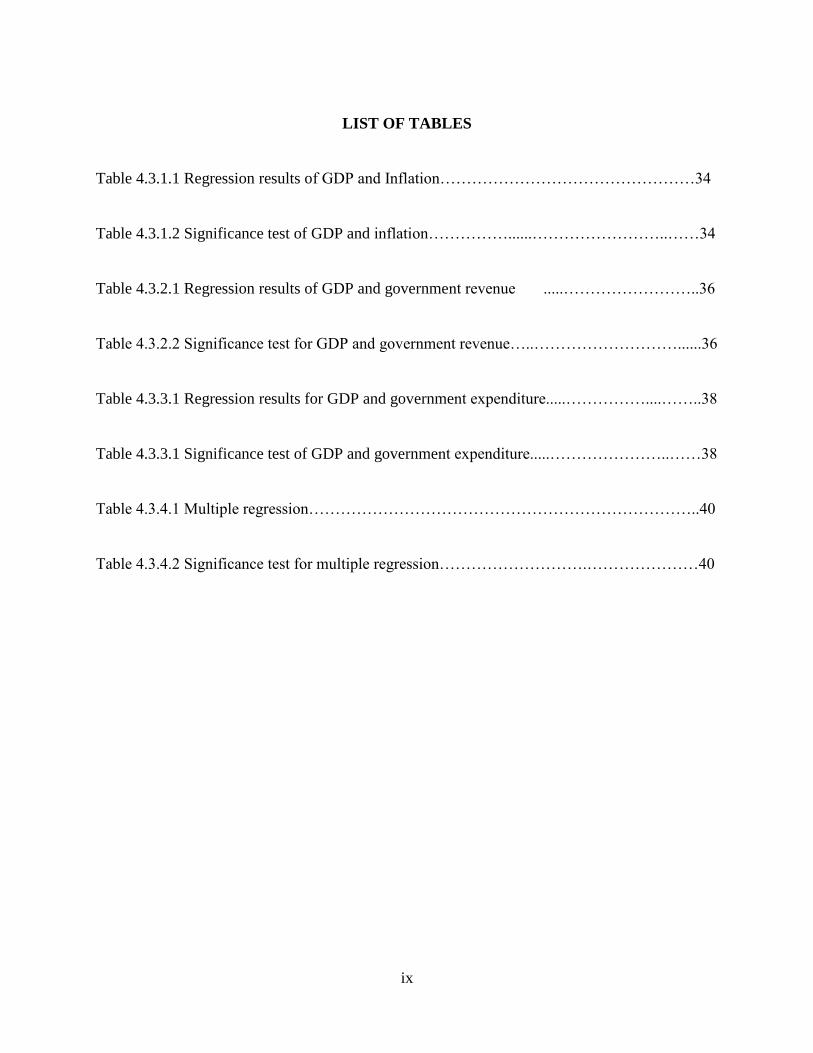
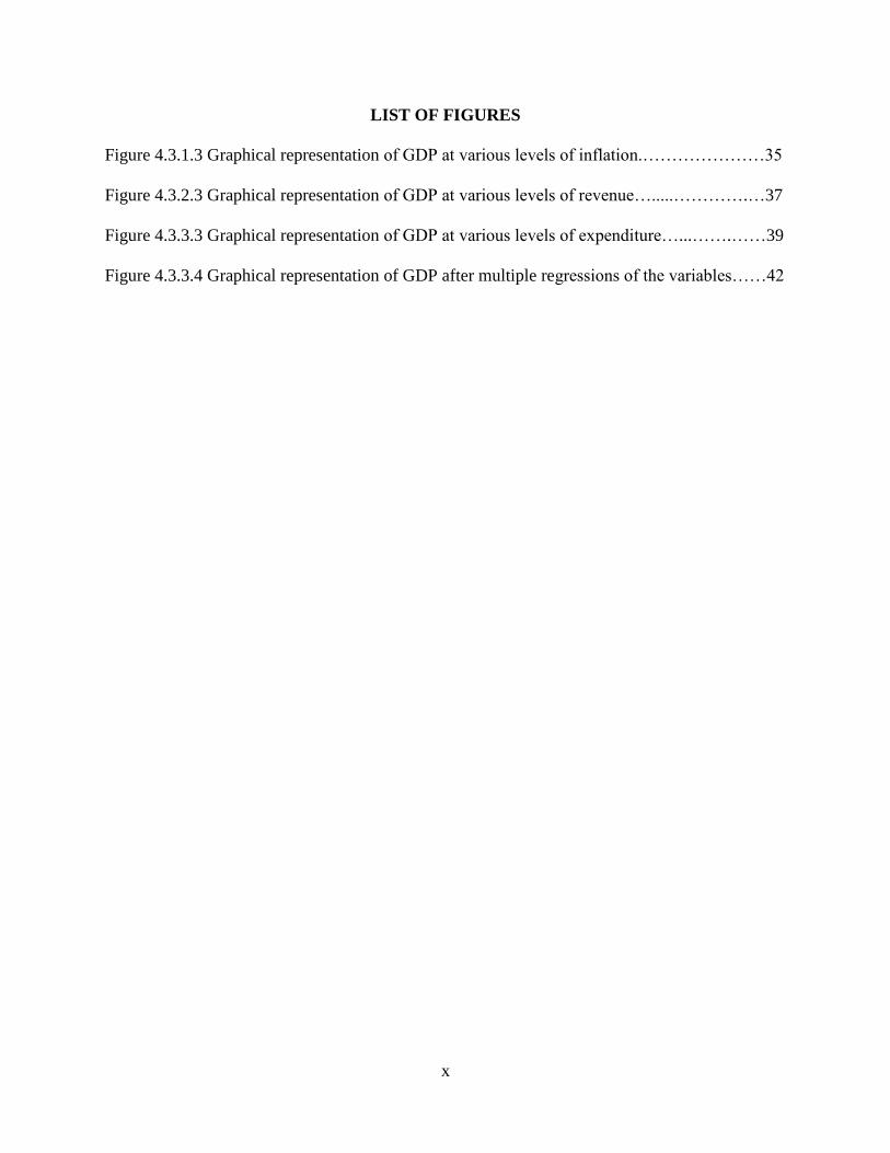


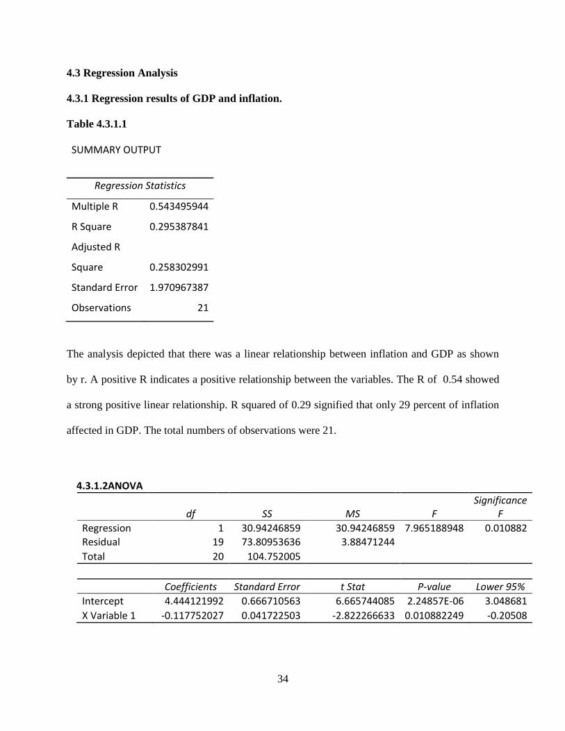
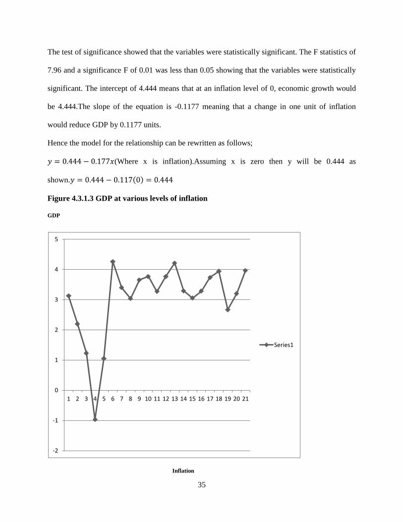
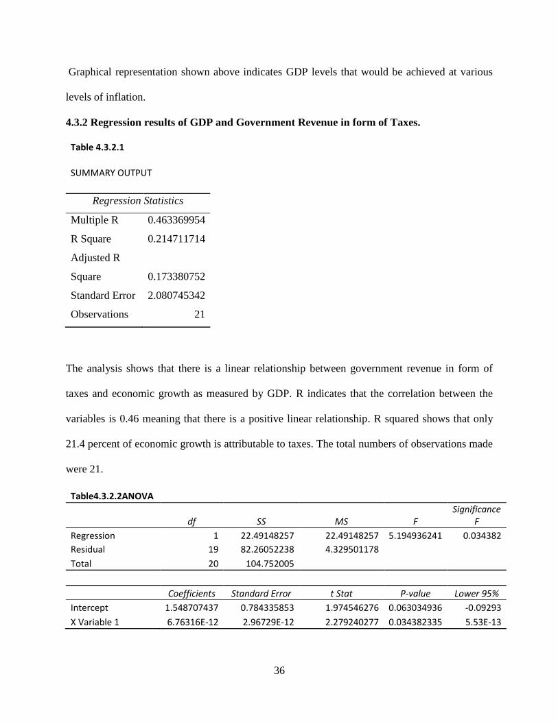
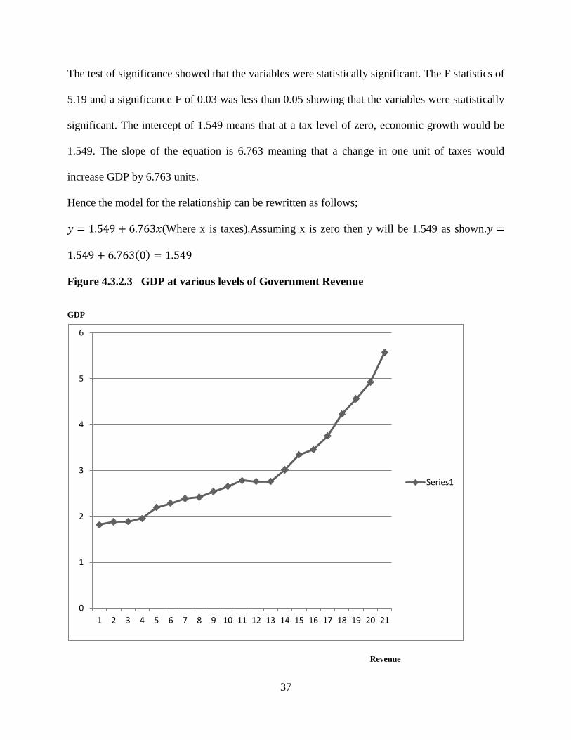
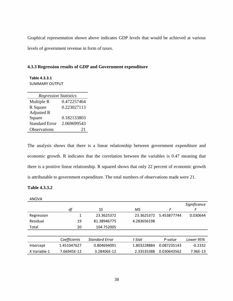
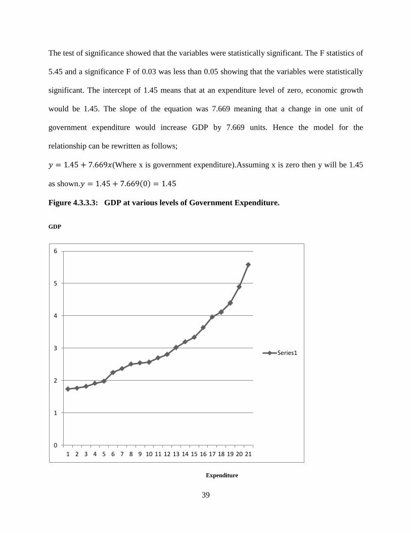
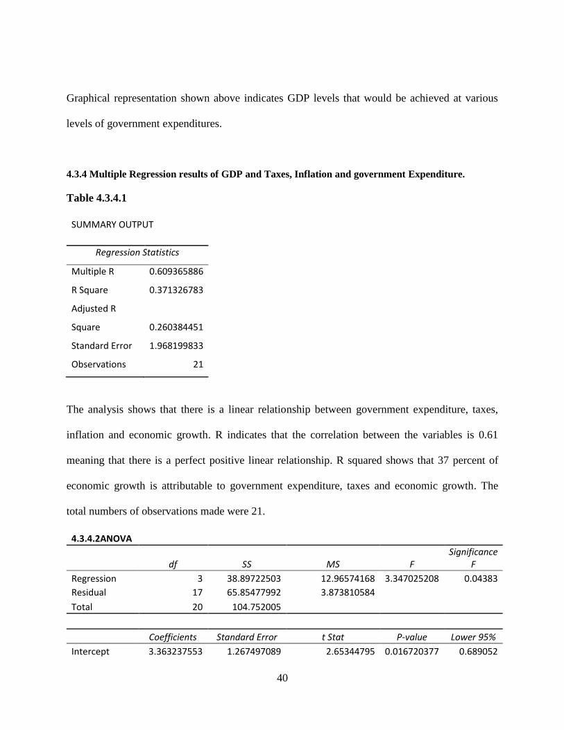
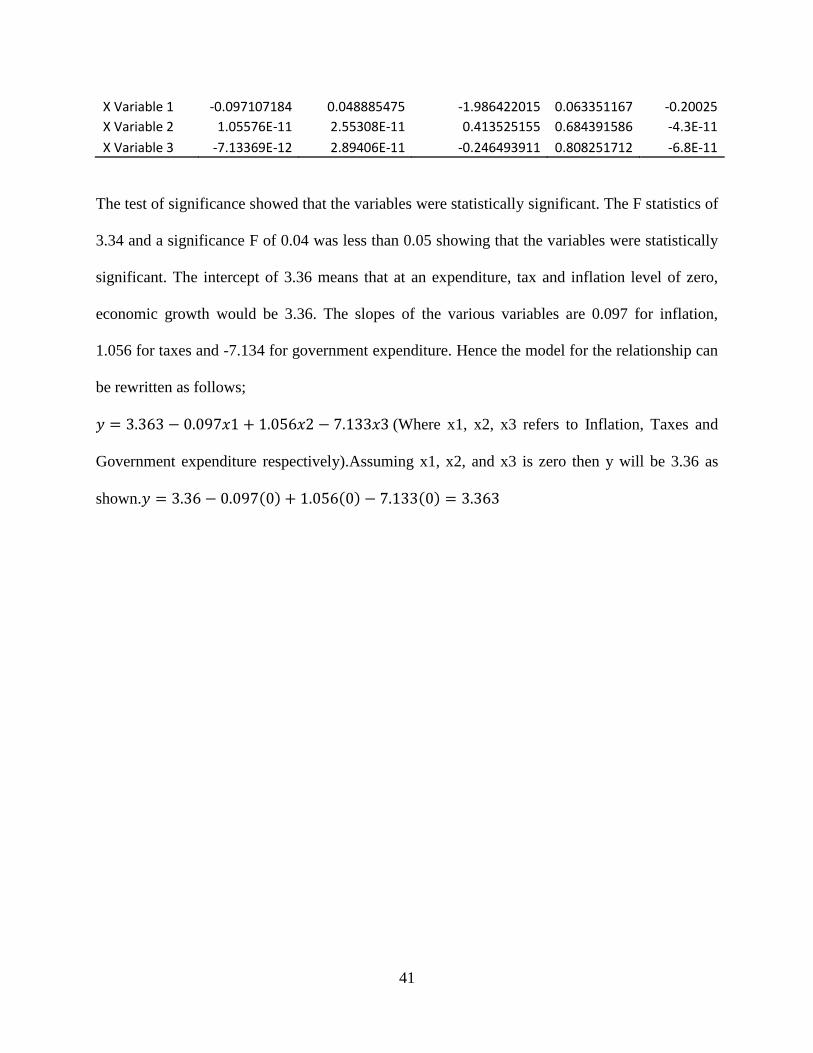
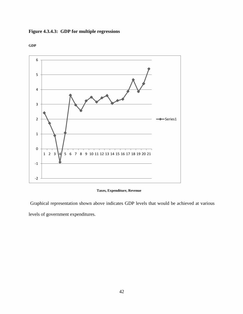
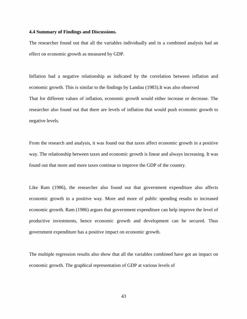


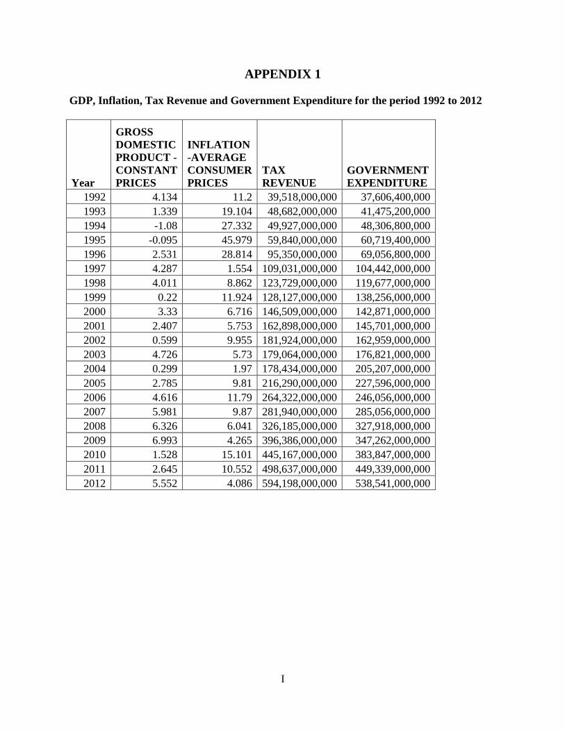
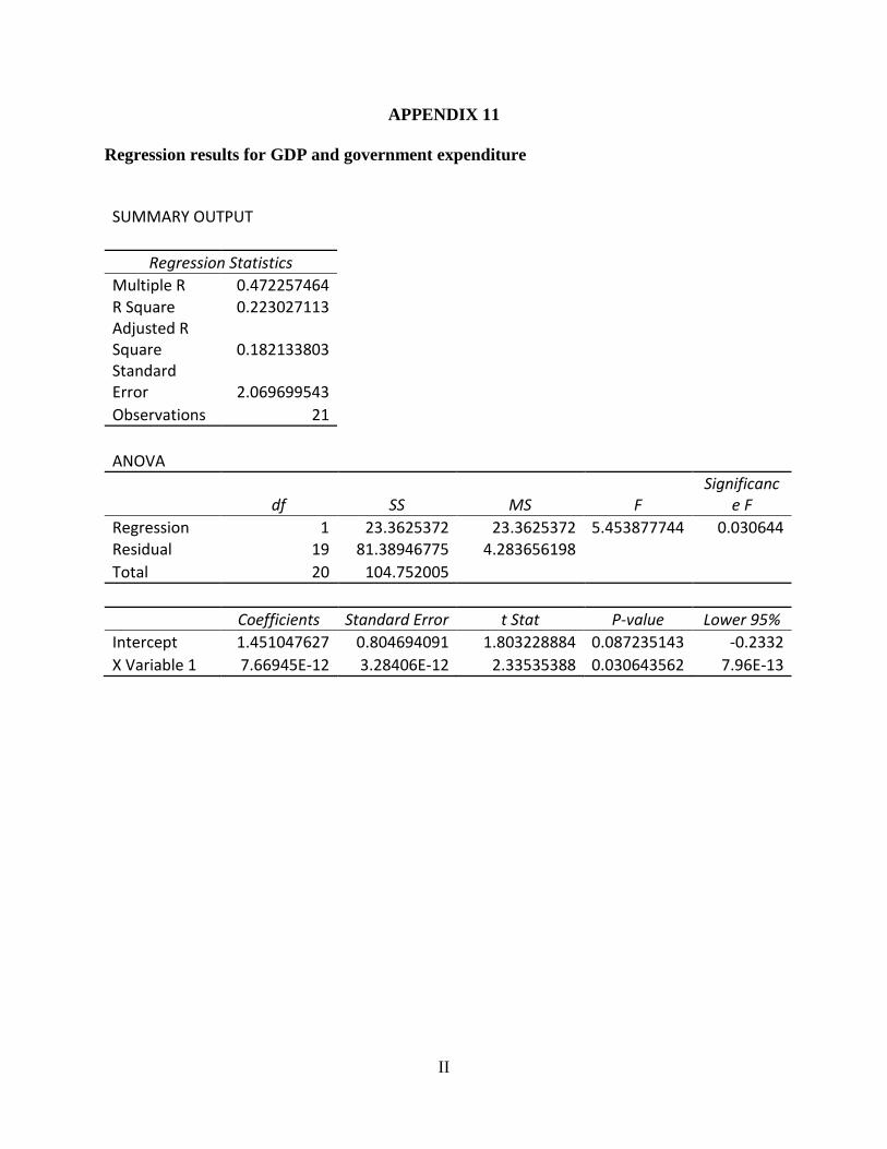
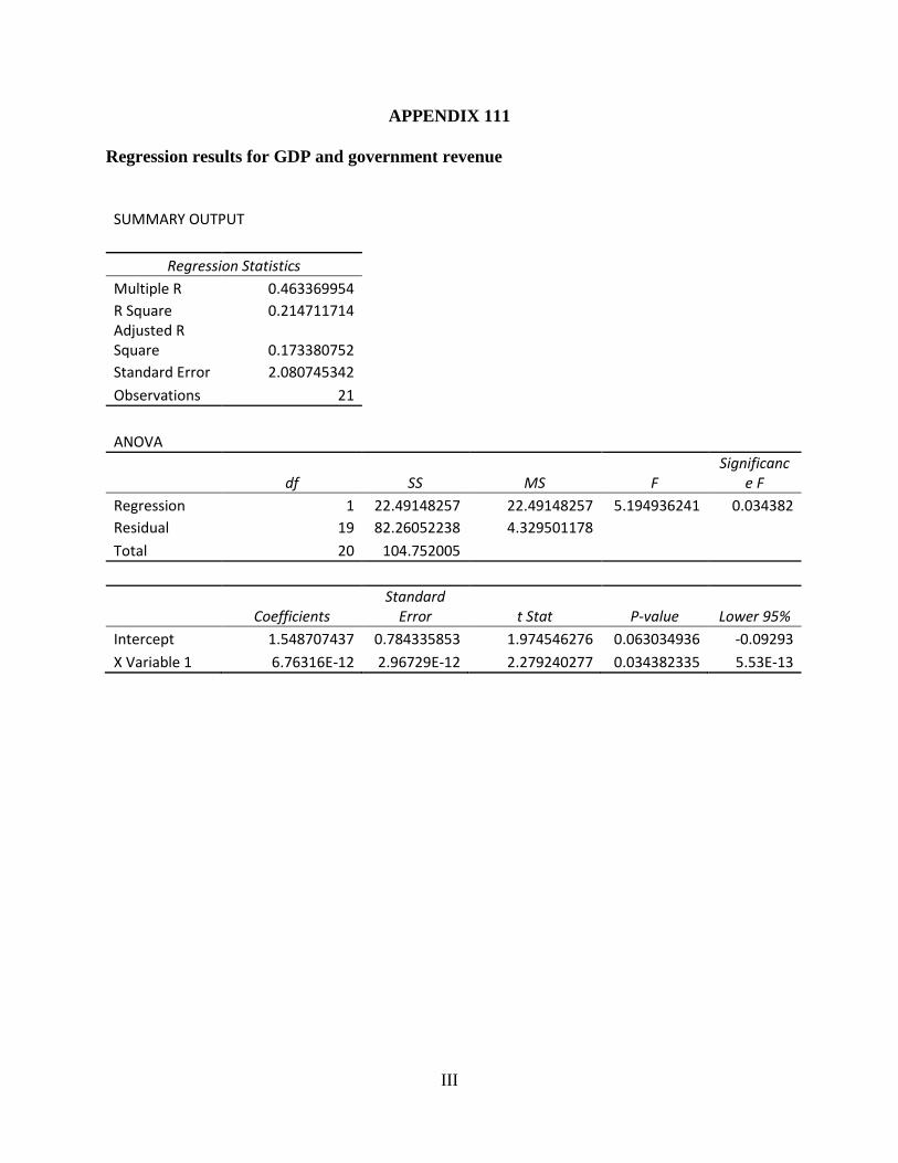
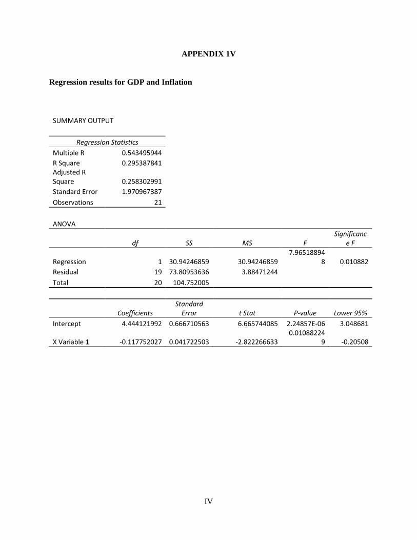
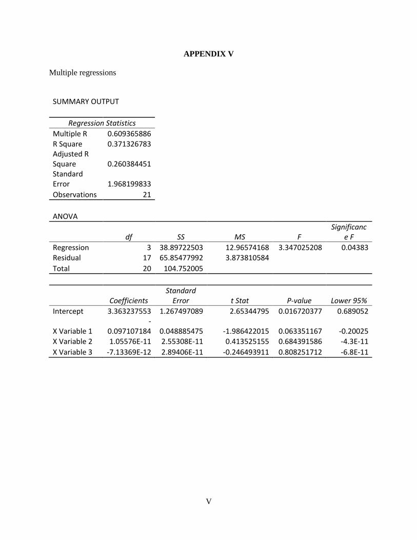


![A Theory for Inflation - UNSW Business School · The Progressive Direct Expenditure Tax as a Tool of Inflation Targeting [A Theory for Inflation: Part II] 9 On Mitigating Recessions](https://static.documents.pub/doc/80x56/5f5061eea041f3044863c176/a-theory-for-inflation-unsw-business-school-the-progressive-direct-expenditure.jpg)


