Page 1
Effects of Gurney Flap on Supercritical
and Natural Laminar Flow Transonic
Aerofoil Performance
Ho Chun Raybin Yu
March 2015
MPhil Thesis
Department of Mechanical Engineering
The University of Sheffield
Project Supervisor: Prof N. Qin
Thesis submitted to the University of Sheffield in partial fulfilment of the
requirements for the degree of Master of Philosophy
Page 2
Page 2
Abstract
The aerodynamic effect of a novel combination of a Gurney flap and shockbump on
RAE2822 supercritical aerofoil and RAE5243 Natural Laminar Flow (NLF) aerofoil is
investigated by solving the two-dimensional steady Reynolds-averaged Navier-Stokes
(RANS) equation. The shockbump geometry is predetermined and pre-optimised on a
specific designed condition. This study investigated Gurney flap height range from 0.1%
to 0.7% aerofoil chord length. The drag benefits of camber modification against a retrofit
Gurney flap was also investigated. The results indicate that a Gurney flap has the ability
to move shock downstream on both types of aerofoil. A significant lift-to-drag
improvement is shown on the RAE2822, however, no improvement is illustrated on the
RAE5243 NLF. The results suggest that a Gurney flap may lead to drag reduction in high
lift regions, thus, increasing the lift-to-drag ratio before stall.
Page 3
Page 3
Dedication
I dedicate this thesis to my beloved grandmother Sandy Yip who passed away during the
course of my research, thank you so much for the support, I love you grandma. This
difficult journey would not have completed without the deep understanding, support,
motivation, encouragement and unconditional love from my beloved parents Maggie and
James and my brother Billy. I am indebted to my high school best friend who has
supported me over the last few years, Tapiwa Only Chidongo. I would like to thank Ben
Hinchliffe, my friend and co-worker, for the entertaining technical discussions,
encouragement and support. I would like to express my thanks to friends and colleagues
who offered support and guidance through this difficult time.
Page 4
Page 4
Acknowledgements
First and foremost, I would like to express my sincere gratitude to my supervisor Prof.
Ning Qin for all his encouragement, valuable comments, motivation and advice
throughout the research study. I would like to thank Airbus UK and ESPRC for the
financial support.
I would like to acknowledge and thank the Advanced Simulation Research Centre for
allowing me to perform my simulations on their cluster computer and providing any
assistance requested. A big thank you to Nathan Harper for the IT support.
I must also thank my industrial supervisors and Project Co-ordinator from Airbus, Dr
Stefano Tursi and Dr Mahbubul Alam and Murray Cross, for the project management and
project direction support. I would like to express my deepest gratitude to Ian Whitehouse
and Norman Wood, aerodynamics experts from Airbus, for all encouragement and
technical support. I have learned so much from you both.
Page 5
Page 5
Contents Page
1. INTRODUCTION - PROBLEM .................................................................................................. 6
1.1 AIM ............................................................................................................................................ 7
1.2 OBJECTIVES ................................................................................................................................ 7
1.3 PROJECT PLANNING ..................................................................................................................... 8
2. LITERATURE REVIEW ............................................................................................................ 9
2.1 FLOW CONTROL .......................................................................................................................... 9
2.2 SHAPING ................................................................................................................................... 13
2.3 GURNEY FLAP ........................................................................................................................... 16
3. RESEARCH METHODOLOGY .............................................................................................. 31
3.1 RESEARCH METHODOLOGY ....................................................................................................... 31
3.2 GOVERNING EQUATION ............................................................................................................. 33
3.3 NUMERICAL METHOD................................................................................................................ 35
4. INVESTIGATIONS AND DISCUSSION ................................................................................. 42
4.1 SUPERCRITICAL AEROFOIL (VALIDATION) ................................................................................. 42
4.2 SUPERCRITICAL AEROFOIL GURNEY FLAP STUDY ...................................................................... 53
4.2.1 Lift constrained investigation ............................................................................................ 53
4.2.2 Camber-line and Gurney Flap investigation ....................................................................... 62
4.2.3 Angled/tilted Gurney Flap investigation ............................................................................ 75
4.2.4 Shockbump and Gurney Flap............................................................................................. 80
4.3 NATURAL LAMINAR FLOW AEROFOIL AND SHOCKBUMP (VALIDATION) ..................................... 97
4.4 NATURAL LAMINAR FLOW AEROFOIL WITH SHOCKBUMP AND GURNEY FLAP .......................... 113
5. CONCLUSION.......................................................................................................................... 127
6. FUTURE WORK ...................................................................................................................... 129
7. REFERENCES .......................................................................................................................... 131
Page 6
Page 6
1. Introduction - Problem
In the current, highly competitive and economically uncertain air transport industry, cost
is one of the main obstacles. The cost is contributed from several sources, such as fuel
price and material cost, of which both are constantly rising. The government also imposes
penalties on high greenhouse gas emission. In order to tackle these problems, aircraft with
higher fuel efficiency are necessity.
At the cruise condition of a typical airliner the biggest problem is drag. Although these
aeroplane are cruising at a transonic region, due to the curvature of the aerofoil, the flow
accelerates on the upper surface and results in a velocity higher than Mach 1 over the
aerofoil. This causes a shock to form on the wing, which reduces the effectiveness of the
aerofoil by wave drag (pressure drag due to compressibility effects) and leads to flow
separations.
Shock is a major obstacle during transonic flight, any form of shock alteration (i.e. delay,
weakening) is beneficial. This study looked deeply into the application of Gurney flap at
the transonic condition. Gurney flap is a well known flow control device in the motor
sport industry for drag reduction and down force increment. Its usage is not limited to
only the automotive, there are extensive studies demonstrating the benefits of this device
for aircraft in take-off and landing configuration, however, there are limited publications
available on the transonic condition. In a recent publication, Yu et al (2011)[14] suggested
that a Gurney flap may delay shock during cruise.
Page 7
Page 7
The main aim of this project is to provide a novel device(s)/system(s) with the means of
flow control to reduce drag (especially during cruise condition) and enhance aerodynamic
performance. Thus, ultimately providing a positive and beneficial impact to the
environment.
1.1 Aim
- Provide a novel solution(s) to tackle the current transonic flow problem and
improve aerodynamic performance through the flow control method, with appropriate
verification and validation.
1.2 Objectives
- Literature review on the current flow control device/ system, identifying areas which
require further development. Conclude with a firm direction of research.
- Investigate, explore and understand the fluid behaviour on the chosen area of flow
control. Establish hypothesises with a cause and effects. This includes experimental
analysis, verification and validation.
- Explore and develop a novel flow control method/ system for the transonic
aerodynamic condition.
- Estimate the beneficial impact and contribution.
Page 8
Page 8
1.3 Project Planning
This research project uses a scientific approach to investigate and finalise its results, and
Computational Fluid Dynamics (CFD) simulation as the experimental tool. This approach
consists of three stages: hypothesis – the predicted and expected outcome, observation –
the results/data, analysis – analysis of obtained data and relationship – discussion of the
relationship between obtained data and hypothesis.
There are four main, interrelated phases for this research project: the literature review of
aerodynamic theory (flow control devices), design, simulation/experiment and
optimisation. The initial phase of background investigation provides a solid foundation
for the project’s directions, goals and aims. The next stage is the design of flow control
device(s) and its initial effects prediction. The third stage involves experimental analysis.
The final stage is to conclude, validate the proposed predictions and provide optimisation
of the design. The overall processes of the project are illustrated in the flow chart below
(figure 1.1).
Figure 1.1: Design Process Structure
Literature Review
New Ideas/ Design
CAD Model
Computer Simulation
Optimisation
Theoretical Prediction
Page 9
Page 9
2. Literature Review
2.1 Flow Control
The topic of flow control is a broad and important subject, it can be defined as the ability
to manipulate a flow field (fluid – including liquid and gases) to perform a desired need
of beneficial requirement. Flow control can be defined into two main types; Passive and
Active. Passive devices are usually a one-off installation and require no external source
of power or energy. These devices will only generate the desire effect during the specific
designed condition. Therefore, they are cheap to equip but they are not adaptable or
flexible in the flow control and causes extra parasitic drag when they are not in use. On
the other hand, Active Flow Control system is more flexible and adaptable in all
conditions, therefore no or very little parasite drag in undesired condition but cost penalty
will occur due to energy consumption. These devices or systems will only perform will
the aid of external power/ energy. Therefore, it is necessary to consider that the benefits
gained by the effective control device must be greater than the cost required by the device.
In order to achieve the desired performance from a particular flow control device/ system,
engineers must pay extra attention to understanding the problem that they encounter. It is
important to provide the best method to resolve such undesired flow conditions. Therefore,
it is necessary to have a clear motive or goal and have a good knowledge of different
types of flow control mechanisms with their possible achievements. [20]Typically, these
goals can be categorised into three distinctive topic: Transition Delay/ Advancement,
Separation Prevention/ Provocation and Turbulence Suppression/ Enhancement. They all
have some degrees of influence features in either Drag Reduction, Lift Enhancement,
Mixing Augmentation or Noise Suppression. For a more detailed breakdown of the flow
Page 10
Page 10
Flow-Control Strategies
Passive Active
Reactive
Feedback
Optimal Control
Dynamical Systems
Physical Model
Adaptive
Feedforward
Predetermined
control classification, energy expenditure and the control loop involved can be used to
distinguish.
Figure 2.1 [20]Classification of flow-control strategies.
Therefore flow control can be defined as Active and Passive, below is a list of flow
control devices for various applications;-
Drag Reduction
- Winglets / Wingtip fences
- Riblets
- Shockbump
Separation Control
- Wing Fences/ Stall Fences/ Boundary Layer Fences/ Vortilon
- Vortex Generators
Page 11
Page 11
- Gurney flap
- Passive Suction (Velocity Profile Modifiers – changing the 𝜕2𝑢
𝜕𝑦2|𝑦=0
to negative)
- Moving walls (turning cylinder)
- Turbulator
- Passive Blowing through leading edge slats and trailing flaps
- Delta Wing
Transition Control
- Wall Motion (Compliant Coating)
- Deturbulator
- Suction
- Shaping => aerofoil profile
- Wall heating/ cooling
Lowering/ affects the near wall viscosity
- Surface heating for liquid/ surface cooling for gas
- Surface-film boiling
- Cavitation
- Sublimation
- Wall injection of lower/ higher viscosity fluid
- Shear thinning/ thickening addictive
Page 12
Page 12
Other Flow control devices
- Leading Edge Cuffs
- Stall Strips
- Leading Edge Slat
- Fixed Slot
- Dog tooth leading edge
- Notched leading edge
- Dimples
Page 13
Page 13
-0.2
-0.15
-0.1
-0.05
0
0.05
0.1
0.15
0.2
0 0.2 0.4 0.6 0.8 1
y
x/c
Aerofoil
RAE5243 Aerofoil
-0.2
-0.15
-0.1
-0.05
0
0.05
0.1
0.15
0.2
0 0.2 0.4 0.6 0.8 1
y
x/c
Aerofoil
RAE5243 Aerofoil
Leading Edge
2.2 Shaping
The wing of an aircraft provides lift, enabling it to fly. Aerofoil is the term used to
describe the cross-section shape of a wing. The aerofoil design is critical, any changes to
the profile can cause substantial effects on the performance of lift, drag and pressure
distribution of the wing.
[39][40]Aerofoil Nomenclature
Figure 2.2.1 Aerofoil nomenclature
The front of the aerofoil is called the Leading Edge and rear of the aerofoil is known as
the Trailing Edge. The distance between the Leading Edge and Trailing Edge is described
as a Chord. The length of the aerofoil, normal to the cross-section from one end to the
other, is called the span. The camber of an aerofoil is usually described as a percentage
Thickness (t)
( Camber (h)
Chord line (c)
Midline / Mean Camber line
Camber line
Trailing Edge
Page 14
Page 14
or a ratio, it is the maximum displacement of mean camber line from the chord (h/c). The
Mean Camber Line or Midline is the locus of centre point of the straight lines
perpendicular across the chord. Thus, the camber line is the bisector of the aerofoil profile
thickness distribution from the leading edge to the trailing edge. The Mean Camber Line
or Midline is commonly describe as the Camber Line in some text books.
Transonic Flight Regime
In a transonic flight regime, this is usually between a Mach number of 0.8 to 1.0, this is
the condition in which the velocities of flow exist, surrounding and flowing past the
aircraft that are concurrently below, at, and above the speed of sound. It is defined as the
range of speeds between the critical Mach number, when the local Mach is at or above
supersonic and the freestream Mach number remains subsonic.
The term Critical Mach (Mcr) describes the freestream Mach number at which a local
Mach equal to 1 is first obtained. The aircraft may be flying with a freestream Mach
number of less than 1. However, due to the curvature of the aerofoil, the flow is
compressed and accelerated. Thus, the local Mach number could be much higher than the
freestream velocity. The local peak Mach number is also the point of minimum surface
pressure. By travelling above the critical Mach number, the aerofoil will experience
localised shock and an increase of pressure drag. For jetliners, thickness-to-chord ratio
(t/c) is usually between 0.1 and 0.15. The thinner aerofoil provides a higher critical Mach
number.
In the transonic cruise condition, the occurrence of shockwave increases drag of the
aerofoil. The sharp pressure increases across the shock, creating a strong adverse pressure
Page 15
Page 15
gradient, which results in flow separation. The free-stream Mach number at which Cd
begins to increase rapidly is defined as Drag-divergence Mach number (Mdrag divergence);
Mcr < Mdrag-divergence < 1.
Supercritical Aerofoil
Supercritical aerofoil is a specially designed aerofoil, targeting performance enhancement
at transonic Mach number conditions. Supercritical aerofoil generates less drag in
comparison to conventional aerofoil by shaping the pressure distribution. This type of
aerofoil features a flatter upper surfaces, which allows a more constant suction to be
distributed across the aerofoil, causing a weaker shock and delayed shockwave, hence,
drag reduction.
Figure 2.2.2 [21]Conventional vs Supercritical Aerofoil
Page 16
Page 16
Natural Laminar Flow aerofoil
[20]The Natural Laminar Flow aerofoil (NLF) uses the benefits of lower skin friction at
the laminar boundary layer, which implies lower drag. However, its main challenge is to
maintain at the laminar boundary layer.
According to the Rutan Voyager’s unrefuelled flight, it was equipped with NLF to 50%
chord. Depending on the shape, angle of attack, Reynolds number, surface roughness and
other factors, the boundary layer either becomes turbulent shortly after the point of
minimum pressure or separates first then undergoes transition. There are many limitations
to this device, such as: crossflow instabilities and leading edge contamination on swept
wings, insect and other particular debris, ice formation, high unit Reynolds numbers at
lower cruise altitudes, and performance degradation at higher angles of attack due to the
necessarily small leading edge radius of NLF aerofoils.
The boundary layer that is kept laminar to extremely high Reynolds numbers is very
sensitive to environmental factors such as roughness, freestream turbulence, radiated
sound and so forth. But the flow can be made reliable and durable with careful and
conscientious design.
2.3 Gurney Flap
Gurney flap, it is a high lift separation control device; a small simple flat plate positioned
perpendicular to the trailing edge of the aerofoil, pointing toward the high pressure
surface. Such devices have existed since the 1930s, it was first patented by E.F. Zaparka
in the USA[16]. Zaparka not only pioneered the static version but also suggested a movable
Page 17
Page 17
version of the mini flap. It was not put into practical use until late 1960s, when Daniel
Gurney installed the horizontal plate pointing upward to the rear spoiler end of his Indy
500 cars to increase down force and reduce drag. It also provided additional benefits to
cornering and straight-away speed.
Apart from its
application in a conventional fixed wing vehicle, this device is also extensively used in
rotary wing aircraft to increase their stabiliser effectiveness. The first helicopter equipped
with a Gurney flap was the Sikorsky S-76B; it was installed on the trailing edge of the
tail stabiliser (NACA 2414) to promote maximum upward lift [1]. Gurney flaps are also
used in wind turbines to increase the output, but the separated unstable flow behind the
flap may lead to noise level increment. These examples are all related to low Mach
number flows. The Gurney flap was first introduce to aerospace by Liebeck (1978)[2].
Later, Lockheed filed a patent in 1985, claiming that a small wedge flap at the trailing
edge improves lifts and reduces drag during cruise condition [18]. The predecessors’ work
led Henne (1990)[17] into his divergent trailing edge (DTE) invention. Some viewed the
DTE as a derivative of the Gurney flap. Such a device was applied to a McDonnel
Douglas MD-11 to enhance its transonic performance.
In general, the addition of Gurney flaps will benefit from an increase of the maximum lift
coefficient (CLmax), and decrease the zero lift angle of attack (α0) [3-8]. But it increases the
nose-down pitching moment (CM) in low angle of attack [3-8]. However, drag may increase
and lift may become enhanced, so it is essential to evaluate the aerodynamic efficiency
(lift-to-drag ratio).
Page 18
Page 18
Gurney flap dimensions are usually described in terms of its height in terms of the chord
length. The principle of the Gurney flap operates by altering the Kutta condition at the
trailing edge. This is because the flap itself alters the stagnation point at the trailing edge
toward the pressure surface, which results in a pressure difference at the trailing edge,
and ultimately provides an increase in lift. With the addition of a Gurney flap, two regions
of separated flow occur. On the immediate aft the flap laid a pair of counter-rotating
vortices, which are alternately shed in a von Kármán Vortex Street. A trapped vortex is
also present and shed in front of the flap. (these vortex locations are purely dependent on
the angle of incident and flow velocity) Therefore, as a result of this downstream vertical
wake, the upper flow (low pressure side) remains attached to the trailing edge, and
ultimately reduces flow separation. These vortices were initially predicted by Liebeck et
al (1978) [2], and later validated by NASA (1988) [9] via a low Reynolds Number
(Re=8,588) water tunnel, using a NACA 0012 aerofoil with 4 different geometries (Figure
2.3.1). The performance of the Gurney flap will diminish at, or after, the stall region.
Figure 2.3.1 [9]Gurney flap models tested.
Page 19
Page 19
This is due to the upper surface flow being fully separated from the trailing edge, and
having the Gurney flap positioned in the vortex wake. Therefore, it could provide an
influence to the flow around the aerofoil. From their study, it was found that the maximum
lift-to-drag ratio can be offered when the Gurney flap height is equal to the boundary
layer thickness.
Liebeck et al (1978)[2] concluded that with a 1.25% chord Gurney flap installed on a
Newman aerofoil, the lift would increase along with a slight reduction in drag. Larger
flap heights were also investigated, which resulted in greater lift increment but were
accompanied by the increase of drag. The drag becomes noticeably substantial when flap
height exceeds approximately 2% chord. It was noted that separation bubbles occur in the
vicinity of the trailing edge at a moderate lift coefficient, or thick trailing edges. Although
the water tunnel test of the Gurney flap from NASA (1988)[9] was several orders of
magnitude different to Liebeck’s initial investigation, the effect was qualitatively agreed.
Kroo (1999)[22] suggested Miniature trailing-edge effectors (MiTEs) are a deployable
version of Gurney flaps that are located at, or near, the trailing edge of an aerofoil, only
to be deployed when required. They are typically segmented into small spanwise elements
that can be individually activated. Jeffrey et al. (2000, 2001)[3][4] also validated Liebeck’s
hypothesis using laser-Doppler measurements at Southampton University (although the
trapped vortex was not clearly displayed). The build-up of pressure immediately in front
of the flap will result in a reduction of the upper surface (low pressure surface) suction
but will produce the same lift. It is believed that the Split and Zap flaps may operate in a
similar principle to the Gurney flap, therefore both flow fields are similar.
Based on the experimental study of Storms et al. (1994)[5], it was shown that the
maximum lift coefficient was increased from 1.49 to 1.96 by the addition of a Gurney
flap to a NACA 4412 aerofoil in low Reynolds Number conditions (Re ~ 2x10⁶). Four
Page 20
Page 20
different flap heights were investigated (0.5, 1.0, 1.5 and 2.0% chord) along with two
deployable configurations with the hinge line forward of the trailing edge by 1.0 and 1.5
flap heights. The drag coefficient was decreased at the maximum lift condition. But drag
increases during low-to-moderate lift coefficients. The results also indicated an additional
nose-down pitching moment associated with the increase of Gurney flap height.
Therefore, a Gurney flap can effectively promote lift of a single-element aerofoil with
very little drag penalty. From the experiment of Bloy et al. (1995)[23], their results showed
that the performance of an aerofoil (NACA 632-215) with a small 45o trailing edge flap
is better than the same aerofoil with a similarly sized Gurney flap. By comparing both
flaps we see that, the 45o flap is less prone to drag. From the range of tested specimens,
the 2% chord 45o flap offered the highest lift, along with the higher lift-to-drag ratio
compared with the entire Gurney flap specimen range. It was concluded that the peak lift-
to-drag ratio of 45o flap is comparable to the aerofoil without flap, but offering a high lift
coefficient. Bloy et al. (1997)[8] carried out an experimental study of 5 different types full-
span 2% chord length trailing edge flaps (45o wedge flap, 45o flap, 90o wedge flap, 90o
Gurney flap and square section – Figure 2.3.2) on a NACA 5414 aerofoil at 52m/s with
Reynolds number 0.57x10⁶. It was concluded that apart from the 45o flap and 45o wedge
flap, which produced slightly less lift enhancement, all the other flaps promoted the
maximum lift in a similar manner. The reduced lift promotion of the 45o flap is caused by
the 1.4% increase in chord length. This study also showed that the 45o flaps provide a
better lift-to-drag ratio across the range of incident angles than a 90o Gurney flap. The
lift-to-drag performance of the test section can be enhanced by the 45o wedge flap. The
maximum lift-to-drag ratio of the 45o wedge flap is slightly less than the plain aerofoil.
Giguere et al. (1995) [24] constructed a variety of experiments and indicated that the
optimum Gurney flap height scale was with the pressure surface boundary-layer thickness
at trailing edge. The optimisation was carried out in respect to the largest lift-to-drag ratio.
Page 21
Page 21
Therefore, in order to achieve to best performance, the Gurney flap should be submerged
within the boundary layer. From the optimum height scaling, a very large Gurney flap
(10 ~ 20% chord) may be expected at low Reynolds number. Although this can be
optimise drag still increases during cruise (low angle of attack). Niu et al. (2010)[25]
provided a numerical solution to the unsteady 2D Navier-Stokes equations, coupled with
a force-element theory to categorise the individual fluid element contributions in the
aerodynamic enhancements from a Gurney flap on a NACA 4412 aerofoil. The numerical
study results were compared and validated with Storms et al’s. (1994)[5] study. It was
indicated that if the Gurney flap is above 2% chord this will result in drastic increases in
lift; this is due to the volume and the surface vorticity. The Gurney flap also produces a
negative source from the surface vorticity to substantially cancel out the drag coming
from the volume vorticity. The lift and drag component is contributed by both volume
vorticity and surface vorticity. Although the contribution of volume vorticity is more
significant, surface vorticity is the key in lift-to-drag ratio optimisation as it contributes
oppositely to both lift and drag.
Figure 2.3.2 Dimensions of trailing-edge flaps from Bloy et al. (1997)[8] tested.
Page 22
Page 22
The benefits of an additional Gurney flap in three-dimension\s is not as promising as the
two-dimensional results. Although the Gurney flap can provide additional lift in all
conditions, in the three-dimensional scenario the increase in Gurney flap height is not as
effective in extra additional lift coefficient as it is for the two dimensional aerofoil section
cases. An extensive low speed wind tunnel analysis on the effect of a Gurney flap on two-
dimensional aerofoil, three-dimensional wings and a reflection plane model was studied
by Myose et al.(1998)[26]. The study included a traditional high lift device, slotted flap,
and addition of a nacelle and fuselage to simulate real life aircraft configuration. There
were four different aerofoil sections used in the study. NACA 0011 and cambered
GA(W)-2 aerofoil were used for a single-element test, GA(W)-2 aerofoil were also
analysed in the two-element test with a 25% chord slotted flap along with a deflection of
10o, 20o and 30o. The following two are used in the three-dimensional analysis, A NLF
0414 straight wing with different spanwise location (inboard, outboard, midspan, full and
clean) and length of Gurney flaps and a tapered NLF 0215 was mounted with a fuselage
and nacelle. The Gurney flap was attached to the trailing edge for all cases, and at in the
slotted flap scenario, the Gurney flap attached to the main aerofoil and the flap itself.
Figure 2.3.3 refers to the aerofoil layout. Figure 2.3.4 describes the test conditions,
including Reynolds number. By comparison with the baseline of clean aerofoil, evidence
shows that the Gurney flap enhanced the maximum lift. But drag penalty occurs,
Figure 2.3.3 The selection of aerofoil used in Myose et al. (2008) [26]’s experiment.
Page 23
Page 23
associated with lift addition. The Gurney flap located at the gap between the slotted flap
(trailing edge element) showed very little performance improvement. On the other hand,
positioning the Gurney flap at the slotted flap showed a much larger improvement in lift.
From the Gurney flap spanwise positioning analysis of the NLF 0414 showed that the
length of the Gurney flap increases the lift and drag linearly, but there are very little
effects in different positions. It is interesting to note that, the three-dimensional analysis
of NLF 0215 tapered wing with both 1.2% chord and 2.5% chord height Gurney flap
experienced almost identical lift and drag increase throughout the range of alpha. The
same characteristics were also displayed for the reflective wing model (NLF 0215 +
fuselage + nacelle).
The wake stabilization technique was used in an attempt to reduce the drag penalty caused
by the addition of the Gurney flap. In Meyer et al.(2006)[7]’s study, they concluded that
the three-dimensional Gurney flap clearly shows drag reduction. They applied slits, holes
and vortex generators individually to the Gurney flap as a wake stabilization device. Both
numerical simulations and wind tunnel experiments were conducted. There were three
different wings (laminar glider aerofoil, High lift profile and a simplified swept constant
chord half model with typical airliner sections) used in the investigation, all with
Reynolds number of 1.0x10⁶ and a Gurney flap height of 0.67% chord. From the slits
Figure 2.3.4 The Gurney flap test condition in Myose et al. (1998)[17] ’ study.
Page 24
Page 24
analysis, it shows that the absolute wake instability which was caused by the buff trailing-
edge was almost completely disappeared. The additional slits led to a significant of 25%
decrease in drag. But the lift is slightly reduced due to the bleed air through the slits,
which made the flap to appear smaller. Nevertheless, at large incidents, the improvement
from the slits is less noticeable. This is because during high incident, the wake from the
aerofoil became strongly asymmetric. Therefore, the drag cannot be further reduced by
instability suppression in the wake. Interestingly, as the absolute instability of the wake
reduced, the wing flutter and noise levels are also reduced. But despite the advantage of
drag reduction from slits, there are penalties; the Gurney flap becomes less rigid and loses
its stiffness. The addition of holes in the Gurney
flap retains the mechanical stiffness and reduces
drag. From Meyer et al’s. (2006)[7] results, it
showed that the flap with additional holes
displayed a better perform drag polar than the
convectional full Gurney flap. There was slightly
less extra lift generated than with a conventional
Gurney flap, this is due to the bleed air. Although the wake instability elimination was
not as thorough as the slit specimen, it is good enough to cause a substantial amount of
drag reduction. Vortex generators (VGs) were also used as a drag reduction device by the
means disturbing the periodic flow field in the wake caused by the Gurney flap. The
geometry of the VGs Gurney flap may be found in figure 2.3.5. As shown from the
diagram, there are two rows of VGs, upper and bottom surface. Because of such
positioning, the wake of the Gurney flap is altered in such a way that the periodic
separation should no longer appear. There is no centre disturbance caused, but only upper
and lower edge, which is fairly different to the holes and slits scenario. With the addition
of VGs, there are no benefits to maximum lift, but a slight reduction in drag. Therefore,
Figure 2.3.5[7] The Gurney flap with vortex
generators.
Page 25
Page 25
this provides an efficient improvement of 0.001 reductions in minimum drag coefficient
when compared with the clean Gurney flap.
A two-dimensional study on various chordwise positions and heights of Gurney flaps
were looked at by Maughmer et al. (2008)[27]. The study consists of both wind tunnel and
computational fluid dynamic analyses. The specimen used was a 12%-thick S903
aerofoil, the S903 section is specially design for laminar flow condition. The experiment
consisted of 3 variables in chordwise locations of 0.90 chord, 0.95 chord and 1.00 chord,
and 3 variable flap height of 0.5% chord, 1% chord and 2% chord, altogether of 9
different configurations. The investigation was carried out in a low speed, low turbulence
wind tunnel, the test were run at 150ft/s (45.72m/s) with a chord Reynolds number of
1.0x10⁶. Two cases were looked at: extended laminar-flow and fixed-transition. The study
concluded that at a higher angle of incident, the influence of the Gurney flap spread
Figure 2.3.6 [27] Change in maximum lift coefficient with varying Gurney flap heights and chordwise
locations. Maughmer et al. (2008)
Page 26
Page 26
increasingly forward. This meant more lift was generated due to a reduced recovery of
adverse gradients on the suction surface, therefore pushing the point of flow separation
to the aft of the aerofoil. For the extended laminar-flow condition, the minimum drag
varies almost linearly with the Gurney flap height, but the flap location has less influence
on the drag component. On the other hand, for the fixed-transition condition, the increase
in drag due to the Gurney flap is less critical. The alterated chordwise position of the
Gurney flap had very little difference on the drag cause when compared with the flap
placed at the end of the trailing edge, but the maximum extra lift generated is reduced and
moved further in toward the aerofoil. This means the lift-to-drag ratio is actually reduced
with position shifted away from the trailing edge. Figure 2.3.6 indicates that as the flap
positioned got closer to the maximum chord, a higher maximum lift was shown.
A study on perforated Gurney flap on NACA 0012 aerofoil was conducted by Lee
(2009)[28], in an attempt to reduce the induced drag. The experiment was carried out at a
low speed wind tunnel, with a Reynolds number of 0.232x10⁶. Extensive amounts of
Gurney flap height (1.6%, 3.2%, 5.5%, 6.7%, 8.8%, 10% and 12% chord) and porosities
(0%, 23%, 40% and 50%, based on the open to closed area of the flap surface) were
investigated. It was shown that by comparing with the convectional flap, the perforation
significantly reduced the wake size and unsteadiness compared with the solid flap. The
experimental data indicated that the perforated flap has a better stall angle delay
characteristic than a solid flap. The stall angle was delayed to 11.5o, 11.8o and 12.7o with
perforation porosities of 23%, 40% and 50% respectively, in contrast with a solid flap the
stall angle is only 10.7o. The suction surface pressure recovery is enhanced by the
perforation. This is due to the disruption of the wake flow behind the flap by jet flow
induced by the perforation. This effect also reduced the flap-induced camber effects. In
Page 27
Page 27
comparison to the convectional Gurney flap, the perforated flap showed an increase in
adverse pressure at the trailing edge location, and induced an earlier boundary-layer
separation from the suction surface. Both suction surface pressure and lower surface
pressure experienced a reduction as the porosities increases. The increase of porosities
will reduce the extent and the near wake intensity/ size, and also the velocity deficit. This
also led to a weaker fluctuating intensity. The perforation condition led to lift reduction
but a reduced nose-down pitching moment in comparison with a non-perforation flap. As
the perforation intensity increases, the maximum lift coefficient, drag coefficient and
maximum nose-down pitching moment coefficient also decreases. The lift decrement of
the flap is caused by the reduction in trailing edge loading. But it is very important to note
that the decrease in drag is more than the loss in lift, therefore, the perforated flap will
lead to more efficiency (higher lift-to-drag ratio) than the conventional Gurney flap.
Beijing University of Aeronautics and Astronautics (2009)[11] investigated the effects of
a plasma actuator Gurney flap (Figure 2.3.7) on a NACA 0012 aerofoil by solving the
Reynolds-averaged Navier-Stokes equation (RANS). The chord length of the aerofoil is
1m and the freestream velocity is 10m/s, with a Reynolds number of 0.684x10⁶. The
plasma actuator is modelled by adding body-force source term to the momentum
equations. The inspiration of this novel device is to solve or reduce the problem of the
induced drag caused by the Gurney flap. This is because the use of a static Gurney flap
will always produce parasitic drag and never retain the same drag coefficient as a clean
aerofoil. The construction of this plasma actuator Gurney flap consisted of a typical single
dielectric-barrier
discharge (SDBD) plasma
actuator placed vertically
to the 0.3% chord (3mm) Figure 2.3.7 [11]Plasma Actuator Gurney Flap.
Page 28
Page 28
thickness trailing edge. The strength of the plasma actuator is represented by a non-
dimensional parameter Dc (this is a representation of the electrical force to the inertial
force). A plasma actuator strength of Dc = 9.14 was investigated. When the plasma
actuator is switch on, its motion will generate a jet stream vertically downward. This
device effectively acts just like the jet Gurney flap but without the complication of
mechanical blowing systems.
From their verification analysis (in lift and pitching moment) with previous research, it
was suggested that the plasma actuator Gurney flap with the strength of Dc = 9.14 is
equivalent to a 0.78% chord conventional Gurney flap and a jet Gurney flap with the
blowing momentum coefficient Cμ ≈ 0.01. The results suggested that the plasma Gurney
flap performs the same way as a conventional Gurney flap, with enhanced maximum lift
and nose-down pitching moment, but with less drag penalty. In comparison to the jet
Gurney flap, the plasma Gurney flap produces the function but with additional benefits
of no moving parts, very fast action and more flexibility. The flow pattern and the loading
variation on the aerofoil obtained from the plasma flap are very similar to the
conventional Gurney flap. The reduction of drag penalty is due to the disappearance of
the von Karman vortex street downstream of the trailing edge. Therefore, the aerofoil
efficiency is improved; achieving a higher lift-to-drag ratio. Also, similar stall
ineffectiveness is also identified in the plasma actuator flap, but it was suggested that its
performance can be improved during post stall by means of an unsteady plasma Gurney
flap, it must act according to the aerofoil’s separated vortex-shedding frequency and the
shear-layer instability frequency. But this required further investigation to verify the
improvement suggestion.
Page 29
Page 29
A recent study by Schuele et al. (2010)[10] looked at the high lift flow control behaviour
with a combination of dielectric barrier discharge (DBD) plasma actuators and the
addition of a Gurney flap. The investigation was conducted at very low Reynolds numbers
of 3,000< Re< 20,000 on a flat and 8% camber plate. In the experiment, DBD was
installed at the leading edge as an active device. A 10% and 20% chord Gurney flap was
employed at the trailing edge as a passive device. It is an alternative form of jet Gurney
flap. Their flap consists of a plasma actuator on the trailing edge. When the actuator is
switched on, a fast jet will be induced. The DBD plasma actuators are to promote the
maximum lift coefficient and increase the stall angle. Therefore, the combined effect for
both controller devices is a cumulative one; the DBD actuators stall delaying mechanism
was also effective in the passively controlled case. The result indicated that from the
conventional semi-empirical models to the very low Reynolds number, the large Gurney
flap (10% chord) provided a 20% increase in the maximum lift and an improvement in
aerofoil efficiency. It was concluded that a Gurney flap generates better improvement in
lift-to-drag ratios at low Reynolds numbers, but the plasma actuators were enhanced at
higher Reynolds numbers.
Rosemann et al (2003)[18] from DLR investigated the effects on a Gurney flap and
divergent trailing edge on VC-opt aerofoil for transonic condition, M = 0.755, Re = 5x10⁶.
The flap heights studied were 0.25%C, 0.50%C, 0.75%C and 1.00%C. Their results
suggested increases of drag at a small angle of attack, but at high lift regions it lead to a
significant drag reduction. It was observed that the effect on pressure distribution is the
development of pressure difference between upper and lower surfaces by the modified
flow condition at the trailing edge. Shock was also shown to have been delayed and is
more resistant to separation.
Page 30
Page 30
The transonic performance of supercritical aerofoil (RAE2822) with a Gurney flap was
investigated by Yu et al (2011) [22]. Their results suggested that with the aid of a Gurney
flap, the shock wave position shifted backward on the suction surface at the same incident
angle and created a wider supersonic region, which significantly increases the lift
coefficient. The lift-to-drag ratio also benefited, with a 10.7% increase in maximum L/D
for a flap h = 0.25% chord length.
From the reviews shown, Gurney flaps can be employed at the trailing edge with a
guaranteed lift increment at the same angle of attack, but they are accompanied by drag
penalties. All variants of the Gurney flap displayed a lift enhancement effect. However,
most of these studies were all conducted in low speed and low Reynolds conditions.
[8]NASA (1988) suggested that altering aerofoil camber, thickness (increase) may lead to
drag reduction. The drag penalty is mostly introduced by the flow separation downstream
of the trailing edge. This device can be very important to high lift configurations, as a
very small device with little weight can enhance a substantial amount of lift. The weight
reduction of traditional high lift devices can lead to less design and manufacturing
complexity. Also, this can be deployed during cruise conditions, as lift increases greater
loads can be transported and a reduced thrust is needed to maintain the lift. Ultimately,
this can provide a large saving in cost. This can also be a safety feature, with studies
showing that a Gurney flap may lead to a delayed stall angle. There are various ways to
enhance the aerodynamic efficiency of a Gurney flap: a less than 0.5% chord for the flap
height, a plasma actuator jet flap and perforated Gurney flap. The work of a plasma
Gurney flap can be expanded, as it requires very little energy input and it is rapid, efficient
(small drag penalty) and flexible. The combination of jet and perforated Gurney flaps can
be quite interesting.
Page 31
Page 31
3. Research Methodology
3.1 Research Methodology
In the broad subject of aerodynamics, in particular for transonic aircraft aerodynamics,
flow behaviours may be analysed in three different ways: Wind Tunnel testing, Numerical
Simulations and actual Flight Tests. Wind Tunnel testing existed over 100 years ago; it is
a way for scientists to simulate flow on the ground in a controlled manner. The wind
tunnel consists of a converging and diverging nozzle to obtain the desired flow velocity
and a working section where the model is placed for testing. This type of analysis often
provides a good estimation of what is happening to the flow and surrounding conditions.
Nevertheless, it requires a high manufacturing cost for an accurate model. During
transonic cruise conditions, the Reynolds number is often very high and a cryogenic wind
tunnel may be used to replicate high Reynolds number conditions. This will often
associate with the penalty of high maintenance and running costs. During the test, models
are mounted on a controller to adjust its angle of attack, and the support rod/ controller
may cause a disruption to the flow, and may lead to inaccurate results. Not to the mention
that the wall effects and turbulence intensity of the wind tunnel are very different to actual
flight conditions. On the other hand, Numerical Simulations, often referred to as CFD
(Computational Fluid Dynamics), provide a solution by solving the governing equation,
and a specific turbulence model. The CAD model is required, then grids/mesh are added
to the surroundings and the calculation is based on the grid. This method is clean and easy
to implement into different flow conditions, turbulent intensity can be adjusted and wall
effects can be neglected, but it may require high computational costs for large calculations.
Both wind tunnel testing and CFD calculation can only produce a ‘very good’ replica of
what is happening in real life situations. This is because during real flight the weather is
Page 32
Page 32
constantly changing which affects temperatures, density, pressures and causes wind, gust
and turbulence. These variables are neglected in both simulations. The most accurate
evaluation is a flight test. This is usually the final stage of evaluation after extensive hours
of CFD and wind tunnel studies. This is the most crucial part as this will give an indication
of what is actually happening during the cruise condition. It is also very dangerous for the
pilots and engineers on board as the aircraft/ aerodynamic modification are in the air for
the first time.
A density based RANS 2nd order finite volume flow solver, TAU, was used to tackle the
fluid problem throughout this report. Geometries/models are constructed and prepared
through RAVEn. Unstructured mesh are used throughout the study and are generated by
SOLAR. The software are accessed remotely via VPN connection to the cluster at ASRC
(Advanced Simulation Research Centre, Bristol, United Kingdom). The simulations and
mesh generations were performed on the HPC (High Performance Computer) cluster.
Shock is a major obstacle during transonic flight, inducing wave drag, potential flow
separation and sudden drag rise. Therefore any means of controlling/weakening/altering
the shock wave for transonic wings is of strong interest. This project emphasised the
behaviour of 2D transonic aerodynamics. This report is split into two interrelated
fundamental bases: Supercritical aerofoil – RAE2822 and Natural Laminar Flow (NLF)
aerofoil RAE5243. Each is then subdivided into further detailed investigation. Both
supercritical and NLF cases are initiated through solver and mesh verification, followed
by wind tunnel data validation.
This project is highly focused on the aerodynamics behaviour triggered by a Gurney flap
at transonic conditions. Investigations such as lift constraint studies, Gurney flap vs
Page 33
Page 33
camber line alteration, shockbump vs Gurney flap and the deflection of the Gurney flap
are discussed in this report.
3.2 Governing Equation[31]
The Navier-Stokes equation is the governing equations of CFD. The equation is derived
from the conversation law of the physical properties of fluid; mass, energy and
momentum.
The Navier-Stokes equations for the three dimensional case can be written in conservative
form as
𝜕
𝜕𝑡∭ �⃗⃗⃗� 𝑑𝑉 = −∬ �̿� ∙ �⃗� 𝑑𝑆
𝜕𝑉𝑉 (3)
�⃗⃗⃗� =
(
𝜌𝜌𝑢𝜌𝑣𝜌𝑤𝜌𝐸)
Where t is the time, V denotes an arbitrary control volume with the boundary V and the
outer normal vector �⃗� . The �⃗⃗⃗� is the vector of the conserved quantities. The density is
represented as ρ, E as the internal energy and u, v, w are the velocities in x, y, z coordinate
directions.
The flux density tensor, �̿�, is composed of flux vectors in the three coordinate directions;
�̿� = (𝐹 𝑖𝑐 + 𝐹 𝑣
𝑐) ∙ 𝑒 𝑥 + (𝐺 𝑖𝑐 + 𝐺 𝑣
𝑐) ∙ 𝑒 𝑦 + (�⃗⃗� 𝑖𝑐 + �⃗⃗� 𝑣
𝑐) ∙ 𝑒 𝑧 (4)
Page 34
Page 34
The 𝐹 𝑐 , 𝐺 𝑐 , �⃗⃗� 𝑐 denotes Flux vectors and superscript c represents Corrective. The ex, ey
and ez are unit vectors in the coordinate directions. The indices i and v denote the inviscid
and viscous contributions respectively. The viscous contributions are neglected when
considering the Euler equations. The viscous and the inviscid fluxes are;-
𝐹 𝑖𝑐 =
(
𝜌𝑢
𝜌𝑢2 + 𝑝𝜌𝑢𝑣𝜌𝑢𝑤𝜌𝐻𝑢 )
,𝐹 𝑣𝑐 =
(
0𝜏𝑥𝑥𝜏𝑥𝑦𝜏𝑥𝑧
𝑢𝜏𝑥𝑥 + 𝑣𝜏𝑥𝑦 +𝑤𝜏𝑥𝑧 + 𝜅𝑙𝜕𝑇
𝜕𝑥)
(5)
𝐺 𝑖𝑐 =
(
𝜌𝑣𝜌𝑢𝑣
𝜌𝑣2 + 𝑝𝜌𝑣𝑤𝜌𝐻𝑣 )
, 𝐺 𝑣𝑐 =
(
0𝜏𝑥𝑦𝜏𝑦𝑦𝜏𝑦𝑧
𝑢𝜏𝑥𝑧 + 𝑣𝜏𝑦𝑦 +𝑤𝜏𝑦𝑧 + 𝜅𝑙𝜕𝑇
𝜕𝑦)
(6)
�⃗⃗� 𝑖𝑐 =
(
𝜌𝑤𝜌𝑢𝑤𝜌𝑣𝑤
𝜌𝑤2 + 𝑝𝜌𝐻𝑤 )
, �⃗⃗� 𝑣
𝑐 =
(
0𝜏𝑥𝑧𝜏𝑦𝑧𝜏𝑥𝑥
𝑢𝜏𝑥𝑧 + 𝑣𝜏𝑦𝑧 +𝑤𝜏𝑧𝑧 + 𝜅𝑙𝜕𝑇
𝜕𝑧)
(7)
The pressure is determined by the equation of state;-
𝑝 = (𝛾 − 1)𝜌 (𝐸 −𝑢2+𝑣2+𝑤2
2) (8)
The temporal change of the conservative variables �⃗⃗⃗� from equation 3 can be derived
from;-
𝜕
𝜕𝑡�⃗⃗⃗� = −
∬ �̿�∙�⃗� 𝑑𝑆𝜕𝑉
∭ 𝑑𝑉𝑉
(9)
Page 35
Page 35
The change of the flow conditions in a control volume V is given by the flux over the
control volume boundaryV related to the size of V. For a control volume fixed in time
and space, the equation (9) can be written as;-
𝑑
𝑑𝑡�⃗⃗⃗� = −
1
𝑉∙ �⃗� 𝐹 (10)
The �⃗� 𝐹 represents the fluxes over the boundaries of the control volume. If the boundary
is divided into n faces, then �⃗� 𝐹 can be represented a;-
�⃗� 𝐹 = ∑ �⃗� 𝑖𝐹𝑛
𝑖=1 = ∑ (�⃗� 𝑖𝐹,𝑐 − �⃗⃗� 𝑖 )
𝑛𝑖=1 (11)
The term �⃗� 𝑖𝐹,𝑐
denotes the inviscid fluxes over the respective face. Hence, in order to
determine the temporal change of the flow quantities in a control volume, the convective
fluxes over the control volume boundaries have to be determined. For upwind schemes
the dissipative terms �⃗⃗� 𝑗 are zero, but for central schemes additional dissipative terms
have to be computed.
3.3 Numerical Method[31]
The basis of the numerical investigation throughout this thesis is performed by DLR TAU
flow solver. The DLR TAU code was developed by Deutsches Zentrum für Luft- und
Raumfahrt e.V. (German Aerospace Center), it was originally created for subsonic and
transonic flow and validated for complex configurations under such Mach ranges. The
code itself is well established and widely used as a general purpose tool for a wide range
Page 36
Page 36
of aerodynamic and aero-thermodynamic problems. The solver enables one to handle
viscous flow around complex objects, from subsonic conditions to hypersonic flow
regimes. TAU code has the ability to couple with other disciplines which enables it to
perform complex multidisciplinary simulations. The Reynolds averaged Navier-Stokes
(RANS) equations are discretised by a finite volume technique via tetrahedra, pyramids,
prisms and hexahedra mesh. Prismatic elements are used for the boundary layer while
tetrahedra mesh are used in inviscid flow regions.
The TAU flow solver is a three-dimensional, parallel, hybrid, multi-grid code. It is
implemented in a finite volume scheme for solving the compressible time-accurate
Reynolds-averaged Navier-Stokes (RANS) equations. The numerical scheme is based on
a second order finite volume formulation, where inviscid terms are computed employing
either a central scheme with scalar or matrix artificial dissipation or a variety of upwind
schemes using linear reconstruction. The flow variables are stored on the vertices of the
initial grid. This type of spatial discretization is called ‘cell vertex’ with a dual metric
which is computed during the pre-processing step. The TAU code uses explicit time
stepping, the multi-step Runge-Kutta scheme and implicit time stepping with a LU-time
scheme. In terms of accelerating the convergence to a steady state, a local time-stepping
concept, a different residual smoothing algorithm and a geometrical multi-grid method
are implemented.
The fluxes calculation may be determined by either an upwind or a central scheme. There
are several flux discretization functions available in an upwind scheme: Van Leer,
AUSMDV, AUSMP, Roe, AUSM Van Leer, EFM and MAPS+. The central method has
two different dissipation models: scalar dissipation and matrix dissipation. The viscous
fluxes for the one equation turbulence models with central schemes are discretised using
Page 37
Page 37
central difference. In the two equation models, the central scheme uses an upwind version
discretisation for their viscous fluxes.
The pre-processor generates a data structure which enables the solver to perform
simultaneously in several sub-domains. In a time-accurate simulation, a global as well as
a dual time-stepping scheme are implemented. The dual time stepping scheme follows
the Jameson Scheme approach, in which the Runge-Kutta scheme is slightly modified to
avoid instabilities while dealing with small physical time steps. The time using dual-time
discretisation can be chosen to be first, second or third order.
The turbulence model implemented in the supercritical aerofoil study is the one-equation
transport model according to the Spalart-Allmaras model (SA)[32]. The model uses only
local quantities for calculating turbulent transport, which makes it suitable for
unstructured methods. The SA model is robust, efficient and able to handle various
flowfield; including scenarios in which small flow separation and reattachment occur. In
this model, the eddy viscosity is directly determined from the single transport equation.
The model has been examined extensively. In the high-lift condition, the SA model
performs similarly to higher-order models and better than algebraic and other one-
equation models [33]. However, in the Natural Laminar Flow aerofoil study the reference
uses a 2 equation model. Therefore, in addition to the one-equation SA model, a 2
equation k-ω Linearized Explicit Algebraic Stress Model was also used in the
investigation and for validation purposes.
Lift Constrained Simulations
This study looked at the Gurney Flap’s performance and behaviour from the prospective
different angle of attack, Mach number and geometrical modification. However, the
Page 38
Page 38
performance comparison is not true if the angle of attack is selected as a base / constant
and drag is a variable. This is because the lift force may differ even it is at the same angle
of attack. The lift constrained simulation was introduced to this investigation, the lift force
will remained constant and other aerodynamics parameter will differ. This makes the
comparison true and feasible. The aerofoil/geometry will be set at its desired lift
coefficient. Prior to lift constrained simulation, a set of different angle attack
aerodynamics data must be obtained. Based on the desired lift coefficient required, the
input angle of attack can be roughly estimated through the data previously obtained. The
principle of the lift constrained simulation is that the simulation is split into two sections:
fixed iteration and auto iteration. The fixed iteration is basically the angle of attack
manually inserted, the calculation continuous until the convergence criteria archives.
Once, the convergence requirement is met, the auto iteration of the angle will start. The
angle iteration calculation is done in steps, it will continue to fluctuate until the desired
lift coefficient and convergence criteria are met.
Example of the lift constrain output.
----------------------------
Markers: 3
Type: farfield
Angle alpha (degree): 2.75
Constant alpha/clift (0/1): 1
Targeted clift: 0.81
Lift iteration period: 200
Lift iteration start: 10000
Name: FARFIELD_ZONE
Angle alpha (degree): 2.7657
Angle alpha (degree): 2.7805
Angle alpha (degree): 2.79399
Angle alpha (degree): 2.80599
Angle alpha (degree): 2.81657
Angle alpha (degree): 2.82588
Angle alpha (degree): 2.834
Angle alpha (degree): 2.84116
Angle alpha (degree): 2.84749
Page 39
Page 39
Angle alpha (degree): 2.85313
Angle alpha (degree): 2.85817
Angle alpha (degree): 2.86275
Angle alpha (degree): 2.86692
Angle alpha (degree): 2.87071
Angle alpha (degree): 2.87421
Angle alpha (degree): 2.87743
Angle alpha (degree): 2.88041
Angle alpha (degree): 2.88314
Angle alpha (degree): 2.88564
Angle alpha (degree): 2.88794
Angle alpha (degree): 2.89003
Angle alpha (degree): 2.89195
Angle alpha (degree): 2.8937
Angle alpha (degree): 2.8953
Angle alpha (degree): 2.89676
Angle alpha (degree): 2.8981
Angle alpha (degree): 2.89933
Angle alpha (degree): 2.90045
Angle alpha (degree): 2.90149
Angle alpha (degree): 2.90244
Angle alpha (degree): 2.90332
Angle alpha (degree): 2.90413
Angle alpha (degree): 2.90487
Angle alpha (degree): 2.90555
Angle alpha (degree): 2.90618
Angle alpha (degree): 2.90676
block end
----------------------------
Flow Solver Setting
Below is the extract of the setting file used in this study for TAU code.
-----------------------------------------------------
SOLVER
-----------------------------------------------------
Inviscid flux discretization type: Upwind
Central dissipation scheme: Scalar_dissipation
Coarse grid upwind flux: Van_Leer
Upwind flux: AUSMDV
Reconstruction of gradients: Least_square
Relaxation ---------------------------------------: -
Relaxation solver: Backward_Euler
Backward Euler ----------------------------------: -
Linear solver: Lusgs
Page 40
Page 40
Linear preconditioner: (none)
Implicit overrelaxation omega: 1.0
Implicit overrelaxation beta: 1
LUSGS --------------------------------------------: -
Sgs stages maximum: 3
Lusgs increased parallel communication (0/1): 1
Lusgs treat whirl implicitly (0/1): 0
Order of upwind flux (1-2): 2
Order of additional equations (1-2): 1
Increase memory (0/1): 1
Solver/Dissipation ------------------------------: -
Matrix dissipation terms coefficient: 0.5
2nd order dissipation coefficient: 0.5
Inverse 4th order dissipation coefficient: 64
Ausm scheme dissipation: 0.25
Limiter freezing convergence: 0
Preconditioning: (none)
Cut-off value: 1.5
Timestepping Start/Stop -------------------------: -
Output period: 100000
Maximal time step number: 100000
Minimum residual: 1e-6
Matching iteration period: 10
Timestep Settings -------------------------------: -
Number of Runge-Kutta stages: 3
CFL number: Variable from 20 to 100
MG-Smoothing ------------------------------------: -
Residual smoother: Point_explicit
Correction smoother: Point_explicit
Correction smooth epsilon: 0.2
Residual smooth epsilon: 0.2002
Correction smoothing steps: 2
Residual smoothing steps: 2
Smoothing relaxation steps: 2
MG Start up -------------------------------------: -
Multigrid start level: 1
References --------------------------------------: -
Reference temperature: 273.15
Reference Mach number: 0.730
Reynolds number: 6.50e+06
Reynolds length: 0.61
Prandtl number: 0.72
Gas constant gamma: 1.4
References --------------------------------------: -
Page 41
Page 41
Reference temperature: 273.15
Reference Mach number: 0.730 (0.67 For NLF case)
Reynolds number: 6.50e+06 (19e+06 For NLF case)
Reynolds length: 0.61 (1 For NLF case)
Prandtl number: 0.72
Gas constant gamma: 1.4
Geometry ----------------------------------------: -
Grid scale: 1.0
Reference relation area: 0.0
Reference length (pitching momentum): 1.0
Reference length (rolling/yawing momentum): 1.0
Origin coordinate x: 0.0
Origin coordinate y: 0.0
Origin coordinate z: 0.0
Turbulence --------------------------------------: -
Turbulence model version: SAO (or Wilcox_k-w in NLF
validation case)
Maximum turbulence production/destruction: 1000
Boussinesq modification for k-production (0/1): 0
Kato Launder modification factor: 1
Turbulence equations use multigrid (0/1): 0
Ratio mue-t/mue-l: 0.1
Maximum limit mue-t/mue-l: 20000
Turbulent intensity: 0.001
Reference bl-thickness: 1e+22
Page 42
Page 42
4. Investigations and Discussion
4.1 Supercritical Aerofoil (Validation)
The purpose of this investigation is to understand the flow behaviour of the RAE2822
aerofoil during transonic conditions. The data obtained will be used as the base control
and then compared with flow characteristics caused by geometric modification. This
section provides verification and validation of the mesh and data for the baseline aerofoil.
Problem definition
Reference temperature: 273.15K
Reference Mach number: 0.73
Reynolds number: 6.50x10⁶
Reynolds length: 0.61
Angle of attack: 2.79o (Corrected angle for CFD, 3.19o used in wind tunnel)
Verification Process
A mesh independent study was constructed to validate the solver’s accuracy on partial
differentiation. The problem definition is based on AGARD’s experimental data [13].
The study analysed the output solution difference in 11 different mesh sizes; ranging from
~20,000 cells to ~4 million cells mesh. The unstructured meshes used are displayed in
figure 4.1.1 and 4.1.2. The farfield from the aerofoil is set to 100 chord length. This is an
industry standard default provide by the software, to eliminate any possible walls effect.
The solver was set to Upwind Backward Euler scheme, and the 1 equation Spalart-
Allmaras turbulence model was applied. The first cell height was set at 1.61x10⁻⁶, in order
Page 43
Page 43
to achieve y+ ≈ 1 as required by the turbulence model. The convergence criteria were set
at 1x10⁶ and maximum of 200,000 iterations.
In table 4.1.1, the results indicate that as the mesh size increases, the output solution will
tend towards being exact. This is because as the mesh size tends toward infinity, the errors
between the partial differentiation with tend toward zero, as the distance between each
node is reduced. This implies that with a very fine mesh output, the solution would be
very similar to the Navier-Stoke equation. However, using infinite size mesh will reduce
the error caused by the governing equations, but result in a time and financial penalty. It
is important to remember that the Navier-Stoke equation only provides a very good
estimate of flow features. It is not an exact solution of the flow physics. It is interesting
to note that the difference in CL and CD between ~50,000 cells grid and ~4,000,000 cells
grid is only 4.46% and 1.62% respectively. Then, by increasing the mesh size to ~250,000
cells, the difference between ~4,000,000 cells for CL and CD is only 1.74% and 1.80%
respectively. Figure 4.1.3 and 4.1.4 indicates lift and drag convergence as more cells are
inserted into the mesh. Thus, the ‘exact solution’ for this scenario is ~4,000,000 cells grid,
with CL = 0.8131, CD = 0.0166 and shock location x/c = 0.5264.
Figure 4.1.2 RAE2822 with 3,873,611 surface
elements grid.
Figure 4.1.1 RAE2822 with 149,986 surface
elements grid.
Page 44
Page 44
Table 4.1.1 – Mesh independent study and comparison with data
Difference between Biggest
and Smallest Mesh
Compared with
Data
Surface Elements CL CD Max y+ Delta-CL Delta-CD W/T CL W/T CD
19,614 0.7226 0.01960 0.9658 11.17% 18.12% 10.01% 16.65%
52,135 0.7772 0.01686 1.0423 4.46% 1.62% 3.22% 0.36%
89,931 0.7894 0.01673 1.0462 2.96% 0.86% 1.70% 0.39%
149,986 0.7959 0.01641 1.0611 2.16% 1.08% 0.89% 2.31%
252,808 0.7993 0.01629 1.0642 1.74% 1.80% 0.46% 3.02%
534,035 0.8043 0.01634 1.0723 1.13% 1.51% 0.16% 2.73%
820,390 0.8075 0.01643 1.0759 0.74% 0.98% 0.55% 2.22%
1,424,841 0.8099 0.01649 1.0793 0.44% 0.62% 0.86% 1.86%
1,808,283 0.8109 0.01652 1.0794 0.32% 0.42% 0.98% 1.66%
2,038,897 0.8113 0.01652 1.0790 0.26% 0.43% 1.03% 1.68%
3,148,634 0.8128 0.01656 1.0805 0.09% 0.18% 1.21% 1.42%
3,873,611 0.8134 0.01659 1.0803 0.00% 0.00% 1.30% 1.25%
0.72
0.73
0.74
0.75
0.76
0.77
0.78
0.79
0.80
0.81
0.82
0 500,000 1,000,000 1,500,000 2,000,000 2,500,000 3,000,000 3,500,000 4,000,000
CL
Number of Surface Elements
RAE2822 - Mesh Independent Study; Lift Coefficient againtist Grid Size
Figure 4.1.3 Graph showing the change in lift coefficient with the increase of surface elements.
Page 45
Page 45
Based on final lift and drag coefficients, several manual local refinements were attempted
at the shock and wake region to reduce computational time with less elements mesh. The
shock location was determined by a filtering algorithm process proposed by Lovely and
Haimes (1999)[29]. A ‘wake line’ was also added to the geometry to provide further
accuracy in a coarse mesh. In the refinement study, 5 different meshes were generated:
“100%” spacing with Wakeline and Shockline (figure 4.1.5); “100%” spacing with
Wakeline and Shockline refinement; “100%” spacing with Wakeline, Shockline
refinement spacing and leading edge and trailing edge refinement; “50%” spacing with
Wakeline and Shockline (figure 4.1.6) and “25%” spacing with Wakeline. From the
simulation produced, in a highly refined mesh it is clear that there is no need for shock
location refinement as the existing grid is already fine enough.
0.0159
0.0164
0.0169
0.0174
0.0179
0.0184
0.0189
0.0194
0.0199
0 500,000 1,000,000 1,500,000 2,000,000 2,500,000 3,000,000 3,500,000 4,000,000
CD
Number of Surface Elements
RAE2822 - Mesh Independent Study; Drag Coefficient vs Grid Size
Figure 4.1.4 Graph showing the change in drag coefficient with the increase of surface elements.
Page 46
Page 46
Figure 4.1.5 RAE2822 aerofoil with manual refinement at shock and wake region, “100%” spacing
with Wakeline and Shockline.
Figure 4.1.6 RAE2822 aerofoil with manual refinement at shock and wake region, “50%” spacing with
Wakeline and Shockline.
Page 47
Page 47
Validation
The CL and CD values obtained from wind tunnel experiments are 0.803 and 0.0168,
respectively [13]. The simulation results are compared with wind tunnel data, along with
surface pressure distribution. The simulation and wind tunnel data pressure plot displays
a positive correlation, however, in figure 4.1.7, the shock location is slightly under
predicted from CFD simulation.
The coarse grid predicted the shock location at x/c = 0.50274, slightly earlier than the
finer grid. This is because as grid size increases the shock position begins to shift. With
the cells spacing getting very close (~800,000 cells and above) the shock position shifting
is also negligible. The shock location difference between 4,000,000 cells and 800,000
cells is only x/c = 3x10⁻³.
Taking the finest mesh solution and comparing with experimental data, the results are
represented in Table 4.1.2. The CFD solution displayed is a very good match with wind
tunnel data, with only 1.30% difference in CL and CD. It is interesting to note that at
~500,000 cells mesh, the CL is the closest match to experimental values. It is only 0.16%
different, but CD show a difference of 2.73%. This is because both CFD and wind tunnel
data will only provide a rough estimate of the flow features; both contain errors. Wind
tunnel testing contains several induced errors, such as wall effects, turbulence intensity,
and temperature fluctuation. The choice of mesh size is critical. Dense mesh can lead to
a more reliable result, however due to the extra cost it is essential to balance the expense
against the potential for errors.
Page 48
Page 48
From all the results shown, the discrepancy between computed and experimental results
are very small. We can therefore conclude that the results obtained from the baseline clean
aerofoil configuration are valid and accurate. However, the pressure distribution on the
suction surface is slightly different than the wind tunnel data. The CFD result displayed
a stronger suction at the leading edge, and a more rapid change in pressure during the
shock region than the wind tunnel data.
Method Alpha CL Δ CL (%) CD Δ CD (%) Shock location
AGARD data[14]
3.19o
0.8030
0.0168
0.5200
S-A model, Tau solver
2.79o
0.8134
1.30
0.0166
1.25
0.5264
Table 4.1.2 Data Comparison
Page 49
Page 49
-1.35
-0.85
-0.35
0.15
0.65
1.15
0.0 0.1 0.2 0.3 0.4 0.5 0.6 0.7 0.8 0.9 1.0Cp
x/c
Surface pressure distribution comparison RAE2822 aerofoil, M=0.73, Alpha = 2.79o, Re = 6.5x10⁶
AGARD 3,873,611 cells3,148,634 cells 2,038,897 cells1,808,283 cells 1,424,841 cells820,390 cells 534,035 cells252,808 cells 149,986 cells89,931 cells 52,135 cells19,614 cells
Figure 4.1.7 Pressure distribution plot: Mesh independent study
Page 50
Page 50
Figure 4.1.8 Mach number contour
Figure 4.1.9 Pressure Coefficient
Page 51
Page 51
Comparison with AGARD’s wind tunnel ( CL = 0.803, CD = 0.0168) indicates a close
relationship with the results of highly refined mesh of CL = 0.813 and CD = 0.0166. The
Δ CL = 1.23%, Δ CD = 1.20%. The shock location from the wind tunnel test is also given
as 0.52 x/c. Therefore, it can be concluded that the results obtained from the baseline
clean aerofoil configuration are valid and accurate. However, the pressure distribution on
the suction surface is slightly different than the wind tunnel data. The CFD result
displayed a stronger suction at the leading edge, and a more rapid change in pressure
during the shock region than the wind tunnel data.
Turbulence Model Selection
There are 5 turbulence models available within the TAU solver: Spalart-Allmaras (SA);
Sparalart-Allmaras modified (SAM); Wilcox kω; Menter Baseline model and the Menter
SST model. The selection process uses a 220,000 cell mesh with a farfield of 25 chord
length. This is because of the high computational cost when using high density mesh. The
simulations are tested with the same conditions described previously, against a different
turbulence model. The residual convergence criteria are set to 1x10⁻⁶ maximum iteration
100,000. The simulation will terminate when any of the criteria reach maximum iteration.
Iterations CL CLp CLv CD CDp CDv CM Max Y+
Spalart-Allmaras (SA) 14192 0.792 0.792 1.048E-05 0.0167 1.108E-02 5.651E-03 -0.175 1.0573
Spalart-Allmaras modified (SAM) 100000 0.795 0.795 -6.235E-06 0.0166 1.108E-02 5.562E-03 -0.176 1.0431
Wilcox kω (2equation) 100000 0.843 0.843 -3.831E-05 0.0193 1.288E-02 6.459E-03 -0.189 1.0584
Menter Baseline model (2equarion) 18866 0.813 0.813 -1.994E-05 0.0178 1.180E-02 5.971E-03 -0.181 1.0631
Menter SST model (2equation) 100000 0.778 0.778 -1.059E-05 0.0163 1.070E-02 5.625E-03 -0.171 1.0413
Table 4.1.3 Turbulence Model Comparison
(i)
Page 52
Page 52
The wind tunnel data for this specific condition is CL = 0.803 and CD = 0.0168.
Table 4.1.3, with the Spalart-Allmaras modified, Wilcox kω and Menter SST turbulence
model displays difficulties in reaching to the set convergence criteria for this specific
mesh. The maximum y+ in all simulation is very close to 1. With a slight alteration to the
mesh, it is possible that future simulations with the previous named turbulence model
might converge within 100,000 iterations. It is also possible that the simulations have not
being running long enough to achieve the convergence criteria. Therefore, the comparison
of ‘Total Run Time’ is rejected. The Spalart-Allmaras model performed fastest, with only
0.0683s per iteration. The slowest model was Menter SST 2 equation turbulence model,
with 0.0791s. Both the SA and the SAM turbulence models provide very similar results
to the experimental data. The SA model showed the best correlation in CD, with just
0.39% difference, but a 1.32% difference in CL. On the other hand, the SAM model
showed an approximately 1% discrepancy for both lift and drag. However, the Wilcox
kω and Menter SST models display a larger difference as well as an increased time
penalty. The SA model is widely used and optimised for the aerospace application [19].
With computation time cost and accuracy taken into account, the SA model was selected.
This model and aerofoil was also selected in Yu et al’s (2011) [14] transonic investigation.
Delta CL Delta CD
Total Run
Time (s)
Time per
Iteration (s)
Spalart-Allmaras (SA) 1.32% 0.39% 970 0.0683
Spalart-Allmaras modified (SAM) 0.94% 0.95% 6930 0.0693
Wilcox kω (2equation) 4.99% 15.09% 7526 0.0753
Menter Baseline model (2equarion) 1.24% 5.77% 1441 0.0764
Menter SST model (2equation) 3.17% 2.83% 7907 0.0791
(ii) – Comparison with experimental data
Page 53
Page 53
4.2 Supercritical Aerofoil Gurney Flap study
The main function of the Gurney flap is lift enhancement. By the use of the Gurney flap,
the same lift can be produced while a reducing of alpha. It was shown by Yu et al (2011)
[14] that in addition, a Gurney flap may increase surface suction and delay shock. This is
an important feature in shock control. The author believes this is an area that can be
further developed and possibly integrated with other shock control devices to enhance the
benefits of drag reduction.
4.2.1 Lift constrained investigation
RAE2822 supercritical aerofoil is used as the baseline, comparing its flow features with
the additional of GF. The height of GF is typically measure in respect to chord length. In
the investigation, 11 different flap heights were used; two upward GFs (0.1%c, 0.25%c)
and seven downward (01%c, 0.2%c, 0.3%c, 0.4%c, 0.5%c, 0.6%c, 0.7%c) GFs. The
thickness of the GFs remained constant. The meshes are generated through SOLAR and
TAU is used to solve RANS equations with one-equation S-A turbulence model for this
problem.
Mesh independent analysis was conducted on Gurney flap cases and clean aerofoil cases
(see previous section), it is clearly shown that beyond 1.8million cells, the solution has
very small alterations and tends toward exact. Then by considering time and computation
cost, the ~1.8million cells grid size was selected for this single point optimisation study.
The simulation parameter is set to cruise condition for the RAE2822, which is M = 0.73,
Re = 6.50 x 10⁶ (based on a chord length of 0.61m) and CL = 0.81. This is because the CL
Page 54
Page 54
obtained at alpha 2.79o is approx. = 0.81. The simulation for clean aerofoil was also re-
run with lift constrained.
Results
Under the lift constrained condition, the 1.8million mesh baseline aerofoil shows a
characteristic of CD = 0.01644, L/D = 49.24, max Mach = 1.297, shock location x/c =
0.524 and alpha = 2.783o.
From the results obtained, in figure 4.2.1.1, it is interesting to note that there is very little
effect on Cp distribution with upward GFs. Slight decrease in lift-to-drag ratio was
observed along with a slight increase in maximum Mach number on the suction surface.
The pressure drag component was shown to have increased as shock strength increased.
An increase of pressure (reduction of suction) was expected on the upper trailing edge of
the upwards GFs, but the graphical results did not represent that hypothesis. However, in
the figure 4.2.1.5 a vortex is clearly seen on the upper surface of the aerofoil. This means
Cp must not be the same as the baseline. The problem may be caused by the trailing edge
stagnation point. Currently, these problems have not been further investigated. It is clearly
seen in Figure 4.2.1.4 for the downward GFs that shock is delayed downstream. In this
particular case, the 0.6%c GF resulted in a maximum drag reduction of 21 counts (Cd =
0.002169). The drag reduction occurred because the shock was weaker and moved further
downstream, which resulted in a large decrease in the pressure drag component.
Figure 4.2.1.3 shows a drag component break down of various GF heights. Vortices were
introduced from the flap, which resulted an increase in CDv. The increase in CDv was
relatively small in comparison to the pressure drag. Therefore, the total drag was reduced.
In this investigation, it indicates that even a 0.1%C height GF, shock is still delayed and
Page 55
Page 55
results in a large reduction in pressure drag. Nevertheless, drag will not infinitely decrease
along with growing flap height. There is an optimum position: when using the flap beyond
optimum height drag penalty will increase. It is believed that this phenomenon may be
caused by the unsteady vortex shedding aft of the flap. In the current investigation of
small GF >1%C, they are set performed using a steady solver and the calculations are
fully converged. This implies the flow is steady.
The surface skin friction plot in figure 4.2.1.2 suggests that shock induced separations are
reduced with downward GF. The immediate after shock, the Cf curve, displays a rapid
decrease in skin friction then increases slowly again. Unlike the baseline case, however
it did not reach zero (when flow separation occurred). Instead it retained a very small
amount of skin friction, and with an increase of flap height, the flow attachment became
firmer. This is seen in figure 4.2.1.2 where the bottom peak travel further upward in
relation to flap height increment. This indicates the flows remain attached when a
downward GF are installed.
For all the GF cases, there are two main vortices shown: clockwise vortex shed
immediately in front of the flap and a large clockwise vortex at the top trailing edge off
the suction surface. In some scenarios, in particular when the flap height is very short,
there is a third vortex, situated under the large vortex aft of the GF, and it is not fully
developed (figure 4.2.1.6). Its development can be seen in the streamline plot. It is
believed that a further increase in flap height will result in the third vortex being fully
developed and combined with the two main vortices. This triggers Karman Vortex Street
and the flow conditions will become unsteady. The addition of downward GF can lead to
the effective angle of attack being reduced. The range of maximum Mach decrease as the
downward GF height increases. The reduction of shock strength and shock delay is
Page 56
Page 56
believed to be caused by the ‘putting force’ coming from the large vortex immediate aft
the flap. The vortex pushes the flow rearward, which enhances attachment flow after the
shock. The vortices created from the flap can be seen as increased camber and effective
chord length.
For the conditions M = 0.73, Re = 6.50 x 10⁶ and CL = 0.81, the optimum flap height is
0.6%c. The 0.6%c suggest a 15.21% increase in L/D, max Mach reduced to 1.249 and
shock was delayed to x/c = 0.588.
From the findings of this study, the small upward GF produced very little effect on
pressure distribution but the overall drag is increased. All downward GF test show
weakening and delay of shockwaves, leading to drag reduction. The angle of attack is
also reduced for any given lift.
The GF is in fact an alteration of the chord: increased camber. In effect, it alters the Kutta
condition of an aerofoil. It is a lift enhancement device and it was expected to have an
increase in L/D. The shock delay caused by the downward GF can be explained as an
effect of the increased camber and accompanied with the rotating vortex at the trailing
edge. It is believed that the rotating vortex provides a “pulling” force to the suction / upper
surface, forcing the flow to attach along the surface. At the same time the flow velocity
is also increased by this force. This explanation requires further evidence and analysis to
support.
Page 57
Page 57
Figure 4.2.1.1 Surface pressure distribution comparison for RAE2822 + Gurney Flaps
-1.35
-0.85
-0.35
0.15
0.65
1.15
0.0 0.1 0.2 0.3 0.4 0.5 0.6 0.7 0.8 0.9 1.0Cp
x/c
Surface pressure distribution comparison;RAE2822 aerofoil Clean, with upward GF and downward GF
M=0.73, CL = 0.81, Re = 6.5x10⁶
Upward GF 0.25%CUpward GF 0.1%CRAE2822 (Clean Aerofoil)Downward GF 0.1%CDownward GF 0.2%CDownward GF 0.3%CDownward GF 0.4%CDownward GF 0.5%CDownward GF 0.6%CDownward GF 0.7%C
Upward GF 0.25%C
Downward GF 0.7%C
Downward GF 0.1%
Downward GF 0.3%C
Page 58
Page 58
Figure 4.2.1.2 Surface skin friction distribution comparison for RAE2822 + Gurney Fla
0.0E+00
2.0E-03
4.0E-03
6.0E-03
8.0E-03
1.0E-02
0.0 0.1 0.2 0.3 0.4 0.5 0.6 0.7 0.8 0.9 1.0
Cf
x/c
Surface skin friction (Cf)distribution comparison;RAE2822 aerofoil Clean, with upward GF and downward GF
M=0.73, CL = 0.81, Re = 6.5x10⁶
Upward GF 0.25%CUpward GF 0.1%CRAE2822 (Clean Aerofoil)Downward GF 0.1%CDownward GF 0.2%CDownward GF 0.3%CDownward GF 0.4%CDownward GF 0.5%CDownward GF 0.6%C
Upward GF 0.25%C
Downward GF 0.7%C
Downward GF 0.2%C
RAE2822 Clean
Downward GF 0.1%C
Page 59
Page 59
Figure 4.2.1.3 Drag Component comparison for RAE2822 + Gurney Flaps
0.000
0.002
0.004
0.006
0.008
0.010
0.012
0.014
0.016
0.018
0.25% upwardGF
0.1% upwardGF
RAE2822(Clean)
0.1%Downward GF
0.2%Downward GF
0.3%Downward GF
0.4%Downward GF
0.5%Downward GF
0.6%Downward GF
0.7%Downward GF
Co
effi
cien
tsDrag Componet for different size of Gurney Flap,
CL = 0.81, M = 0.73, Re = 6.5x10⁶CD CDp CDv
Page 60
Page 60
Figure 4.2.1.4 Bar chart to show the changes in drag for different size Gurney flap
-0.0022
-0.0017
-0.0012
-0.0007
-0.0002
0.0003
0.0008
0.25% upwardGF
0.1% upwardGF
RAE2822(Clean)
0.1%Downward GF
0.2%Downward GF
0.3%Downward GF
0.4%Downward GF
0.5%Downward GF
0.6%Downward GF
0.7%Downward GF
ΔC
DA bar chart to show the ΔCD for different size Gurney Flap,
CL = 0.81, M = 0.73, Re = 6.5x10⁶
Page 61
Page 61
Figure 4.2.1.5 Mach Contour plot and stream plot for RAE2822 with 0.25%c upward Gurney flap
Figure 4.2.1.6 Mach Contour plot and stream plot for RAE2822 with 0.20%c Gurney flap
Page 62
Page 62
4.2.2 Camber-line Modification and Gurney Flap investigation
In the previous section, it showed positive drag reduction with the addition of a Gurney
flap. It is very interesting that a small plate attached to the trailing edge of a wing can
increase a vast amount of performance. The addition of Gurney flap can be seen as a
camber alteration. From results in previous section, for a given lift condition, the Gurney
flap alters the Kutta condition, it increases rear loading and reduces top surface suction in
comparison with the clean aerofoil. The lift enhancement behaviour also suggests the
addition of Gurney flap affects the aerofoil’s effective camber line. This is a form of
trailing edge modification, which alters the effective camber. Therefore, by looking at
the drag produced by the Gurney flap addition and camber-line alteration with the same
lift performance can suggest validation Gurney flap over aerofoil redesign.
The camber-line calculation is obtained from the vortex situated in front of the flap. The
curvature flow travelled outside the vortex was considered as elliptical, this curvature
flow is assumed to be the ‘pressured surface’ as if the Gurney flap not installed. By
approximation, the centre point of the ellipse was obtained, the original camber line are
then modified using the elliptical equation. The distance between upper curve and lower
curve to the camber line retained as the same as the baseline aerofoil. The upper and
lower curve co-ordinates are obtained through the derivative of the camber line, then
generate an equation normal to the camber line, and by inserting the ‘thickness’ (distance).
The surface co-ordinates are then calculated.
The selected Gurney flap geometries are 0.3% and 0.4% chord. Then the two camber-line
modified aerofoils were generated; in respect to 0.3%c and 0.4%c Gurney flap. The
Page 63
Page 63
geometries were simulated at M = 0.73, Re = 6.5 x 10^6, Chord length = 0.61m (based
on AGARD RAE2822 case 9) through TAU, using SA turbulence modelling.
As predicted, the camber modified aerofoil showed approximately the same lift enhanced
behaviour as the Gurney flap. This is shown in figure 4.2.2.1, CL-alpha plot, the cambered
aerofoil and Gurney flap aerofoil laid exactly on top of each. And more interestingly,
figure 4.2.2.3, the Cm behaviour is almost identical for both cambered and flap added
aerofoil. This suggests the Gurney flap and cambered alteration contains similarly
aerodynamic behaviour, this mean CL and Cm can act as a constraint. In terms of drag
coefficient in respect to angle of attack, it is clearly show that the standard clean aerofoil
produces the less drag, the camber modified version is always less drag then retrofit
Gurney flap. This is only valid in reference to angle of attack. The aerodynamics
performance can be seen in figure 4.2.2.4, the addition of Gurney flap or camber
modification clearly shown an increase in L/D ratio. Again, the simulation results it
indicates the camber modified aerofoil contains less drag than the addition of GF.
In Table 4.2.2.1, this is the simulation results of lift constrained scenario, it indicate that
both cambered and Gurney addition generates a positive benefit to the L/D ratio. The
cambered aerofoil (replica of Gurney flap addition ) performed very similar in term of
pitching. However, in terms of drag, figure 4.2.2.1a the cambered version conquers over
the standard Gurney flap. In the drag breakdown, the Cdv remains very similar for all 5
cases, but the Cdp is shows where the difference occurs. And in both figure 4.2.2.7 and
4.2.2.8 indicates camber modified aerofoil delays shock downstream to the very similar
position as Gurney flap can achieve. The main reason for cambered aerofoil in performing
less drag than Gurney flap addition, it is because the reduction or elimination of the two
rotational vortex caused by the Gurney flap. The cambered trailing edge reduces the rapid
Page 64
Page 64
dive sharp corner on the upper surface trailing and the removed of the vertical plate. As
the sharp trailing edge abolished, the flow follows the geometry more easily without
causing such high distribution and resulting in a large rotational vortex. Although, in
figure 4.2.2.10a a vortex exist on the upper surface near the trailing but in comparison to
figure 4.2.2.10d the effective are by far much lessen. The vortex immediate in front of
the flap is caused by the flap as a blockage of flow causing it to redirect and resulting a
vortex. The vortex itself is trapped once it is generated and reached stability, the steam
wise flow will then follow around the vortex, treating it as a wedged trailing edge. The
cambered version already provided the “wedged” curvature for the lower surface, which
implies the rotation vortex is neglected, therefore less energy are wasted.
In this study, the obtained result suggests the modification of camber is more effective
than addition of GF. However, GF can be retro fit to service aircraft, and camber alteration
can be very difficult achieve to an existing wing.
Page 65
Page 65
-0.6
-0.4
-0.2
0
0.2
0.4
0.6
0.8
1
1.2
-5 -4 -3 -2 -1 0 1 2 3 4
CL
Angle of Attack
CL vs Alpha, M=0.73, Re = 6.5 x10^6
RAE2822 Clean
RAE2822_GF0.3%C
RAE2822_Camber(GF0.3%C)
RAE2822_GF0.4%C
RAE2822_Camber(GF0.4%C)
Figure 4.2.2.1, CL vs Alpha
0.00
0.00
0.00
0.01
0.01
0.01
0.01
0.01
0.02
0.02
RAE2822 Clean RAE2822 GF - 0.4%C RAE2822 GF - 0.3%C RAE2822_Camber(0.3%GF) RAE2822_Camber(0.4%GF)
Dra
g C
oe
ffic
ien
t
Angle of Attack
Comparison of Drag Components (CL=0.81, M=0.73, Re = 6.5x10^6)
Total Cd
CDp
CDv
Figure 4.2.2.1a, Comparison of Drag Components (CL=0.81, M=0.73, Re = 6.5x10^6
Page 66
Page 66
Table 4.2.2.1
Lift Constrained; CL = 0.81
Aerofoil Alpha CLtotal CLp CLv CDtotal CDp CDv CM L/D
RAE2822 Clean 2.79 0.809670 0.809647 0.000023 0.016442 0.010815 0.005627 -0.178260 49.243920
RAE2822 GF - 0.3%C 1.727749 0.807683 0.807625 0.000058 0.015393 0.009632 0.005761 -0.206275 52.470714
RAE2822 GF - 0.4%C 1.514209 0.809183 0.809118 0.000065 0.015815 0.010047 0.005768 -0.212099 51.164867
RAE2822_Camber(0.3%GF) 1.740485 0.810958 0.810895 0.000064 0.014853 0.009116 0.005737 -0.205284 54.600084
RAE2822_Camber(0.4%GF) 1.441573 0.810910 0.810836 0.000074 0.014210 0.008403 0.005807 -0.212420 57.065072
Figure 4.2.2.2, CD vs Alpha
0.005
0.01
0.015
0.02
0.025
0.03
0.035
0.04
0.045
0.05
-5 -4 -3 -2 -1 0 1 2 3 4
CD
Angle of Attack
CD vs Alpha, M=0.73, Re = 6.5 x10^6
RAE2822 Clean
RAE2822_GF0.3%C
RAE2822_Camber(GF0.3%C)
RAE2822_GF0.4%C
RAE2822_Camber(GF0.4%C)
Page 67
Page 67
Figure 4.2.2.4, Aerodynamic efficiency (CL/CD)
Figure 4.2.2.3, Cm vs Alpha
-0.3
-0.25
-0.2
-0.15
-0.1
-0.05
0
0.05
-5 -4 -3 -2 -1 0 1 2 3 4
CM
Angle of Attack
Cm vs Alpha, M=0.73, Re = 6.5 x10^6x10^6
RAE2822 Clean
RAE2822_GF0.3%C
RAE2822_Camber(GF0.3%C)
RAE2822_GF0.4%C
RAE2822_Camber(GF0.4%C)
0
0.005
0.01
0.015
0.02
0.025
0.03
0.035
-0.6 -0.4 -0.2 0 0.2 0.4 0.6 0.8 1 1.2
CD
CL
L/D, M=0.73, Re = 6.5 x10^6
RAE2822 Clean
RAE2822_GF0.3%
RAE2822_Camber(GF0.3%C)
RAE2822_GF0.4%C
RAE2822_Camber(GF0.4%C)
Page 68
Page 68
0
0.005
0.01
0.015
0.02
0.025
0.03
0.035
0.04
0.045
0.05
-4 -3 -2 -1 0 1 2 3 4
Dra
g C
oe
ffic
ien
t
Angle of Attack
GF 0.3%C - Comparison of Drag Componets (M=0.73, Re = 6.5x10^6)
RAE2822_GF0.3%_Total CdRAE2822_Camber(0.3%GF)_ Total CdRAE2822_Total CdRAE2822_GF0.3%_CdpRAE2822_Camber(0.3%GF)_CdpRAE2822_CdpRAE2822_GF0.3%_CdvRAE2822_Camber(0.3%GF)_CdvRAE2822_Cdv
Figure 4.2.2.5, GF 0.3%C - Comparison of Drag Components (M=0.73, Re = 6.5x10^6)
Page 69
Page 69
0.00
0.01
0.02
0.03
0.04
0.05
0.06
-4 -3 -2 -1 0 1 2 3 4
Dra
g C
oef
fici
ent
Angle of Attack
GF 0.4%C - Comparison of Drag Components (M=0.73, Re = 6.5x10^6)
RAE2822_GF0.4%_Total CdRAE2822_Camber(0.4%GF)_ Total CdRAE2822_Total CdRAE2822_GF0.4%_CdpRAE2822_Camber(0.4%GF)_CdpRAE2822_CdpRAE2822_GF0.4%_CdvRAE2822_Camber(0.4%GF)_CdvRAE2822_Cdv
Figure 4.2.2.6, GF 0.4%C - Comparison of Drag Components (M=0.73, Re = 6.5x10^6)
Page 70
Page 70
-1.70
-1.20
-0.70
-0.20
0.30
0.80
0.0 0.1 0.2 0.3 0.4 0.5 0.6 0.7 0.8 0.9 1.0
Cp
x/c
Surface pressure distribution comparison;RAE2822 aerofoil Clean, with with Gurney Flap and Camber modification
M=0.73, CL = 0.81, Re = 6.5x10⁶
RAE2822 CleanRAE2822 + GF 0.3%CRAE2822 - Camber (GF 0.3%C)RAE2822 + GF 0.4%CRAE2822 - Camber (GF 0.4%C)
Figure 4.2.2.7, Surface pressure distribution, RAE2822 and modification, M=0.73, Re = 6.5x10^6)
Page 71
Page 71
0.0E+00
2.0E-03
4.0E-03
6.0E-03
8.0E-03
1.0E-02
0.0 0.1 0.2 0.3 0.4 0.5 0.6 0.7 0.8 0.9 1.0
Cf
x/c
Cf surface distribution comparison;RAE2822 aerofoil Clean, with Gurney Flap and Camber modification
M=0.73, CL = 0.81, Re = 6.5x10⁶
RAE2822 CleanRAE2822 + GF 0.3%CRAE2822 - Camber (GF 0.3%C)RAE2822 + GF 0.4%CRAE2822 - Camber (GF 0.4%C)
Figure 4.2.2.8, Cf Surface distribution, RAE2822 and modification, M=0.73, Re = 6.5x10^6)
Page 72
Page 72
a)
b)
Figure 4.2.2.9a, b, RAE2822_Camber(GF_0.4%C) @CL=0.81
Page 73
Page 73
Figure 4.2.2.10a, RAE2822_Camber(GF_0.4%C) @CL=0.81 Figure 4.2.2.10b, RAE2822_Camber(GF0.3%)
@=CL=0.81
Figure 4.2.2.10a, RAE2822_Camber(GF_0.4%C) @CL=0.81 Figure 4.2.2.10b, RAE2822_Camber(GF0.3%)
@=CL=0.81
Page 74
Page 74
Figure 4.2.2.10c, RAE2822_GF_0.3%C @CL=0.81
Figure 4.2.2.10d, RAE2822_GF_0.4%C @CL=0.81
Page 75
Page 75
4.2.3 Angled/tilted Gurney Flap investigation
The performance of Gurney Flap is greatly depending on the length of the flap. The larger flap can
generate more disruptions, which results in larger vortex core both in front and after the flap. However,
if the flap is too larger, the disruption can be too great and causes negative effectives and as well as
Karman’s vortex street. In previous section, the result suggests that s cambered trailing edge is more
effective than conventional vertical drop flap. This brings the interests in investigating the effect on
angled/ tilted Gurney flap. This experiment uses the ‘optimum’ Gurney flap length as a based, then
by applying trigonometry and Pythagoras theorem with the desired tilt angle to determine the flap
dimension. This can be seen in figure 4.2.3.1.
This study uses result obtained in previous sections, which concluded the effective flap length is
between 0.5%c and 0.6%c. The simulation are performed at M=0.73, Re = 6.5 x 10^6 and lift
constrained to CL = 0.81. The 0.5%c Gurney flap geometry were modified through RBF mesh
deformation in small steps (distance of x = 0.0001m) and applied into the simulations. The best
geometry dimension is then obtained by selection. The geometry began with 0.5%c and end with
0.5902%c. Table 4.2.3.1 shows the performance comparison of the specimen test range. The results
indicate that 0.5615%c Gurney flap produced the least drag and this length is selected for the tilted/
angled study.
Figure 4.2.3.1, Tilt Gurney flap - Sketch
Gurn
ey F
lap
vertica
l heig
ht
Extra chord length – x axis
Page 76
Page 76
Four different geometries are used in this study with the constant vertical height and tilted angle of
35o, 45o, 60o and 70o. In order to provide a good comparison, the simulations are conducted in the
same condition, M = 0.73, Re = 6.5 x 10^6, CL = 0.81 and with S-A Turbulence Model. The simulated
result, Table 4.2.3.1, indicates tilted 60o has the most effective performance out of the 4 geometries.
Table 4.2.3.1
CL CD CM L/D
Name Alpha CLtotal CLp CLv CDtotal CDp CDv
RAE2822 Clean 2.7900 0.8097 0.8096 0.0000 0.01644203 0.01081465 0.00562738 -0.1783 49.24
RAE2822 GF - 0.5%C 1.2999 0.8091 0.8090 0.0001 0.01559095 0.00980276 0.00578819 -0.2173 51.89
RAE2822 GF - 0.5164% 1.3000 0.8092 0.8092 0.0001 0.01558985 0.00980093 0.00578892 -0.2173 51.91
RAE2822 GF - 0.5328% 1.3000 0.8092 0.8092 0.0001 0.01558993 0.00980101 0.00578892 -0.2173 51.91
RAE2822 GF - 0.5492% 1.2999 0.8092 0.8092 0.0001 0.01558987 0.00980097 0.00578891 -0.2173 51.91
RAE2822 GF - 0.5533% 1.3000 0.8092 0.8092 0.0001 0.01559078 0.00980185 0.00578893 -0.2173 51.91
RAE2822 GF - 0.5574% 1.2999 0.8092 0.8092 0.0001 0.01558998 0.00980107 0.00578891 -0.2173 51.91
RAE2822 GF - 0.5615% 1.2999 0.8092 0.8092 0.0001 0.01558957 0.00980066 0.00578891 -0.2173 51.91
RAE2822 GF - 0.5656% 1.3000 0.8092 0.8092 0.0001 0.01559017 0.00980124 0.00578893 -0.2173 51.91
RAE2822 GF - 0.5820% 1.2999 0.8092 0.8092 0.0001 0.01559008 0.00980117 0.00578891 -0.2173 51.91
RAE2822 GF - 0.5902% 1.2999 0.8092 0.8092 0.0001 0.01559001 0.00980111 0.00578890 -0.2173 51.91
Table 4.2.3.2
CL CD CM L/D
Name Alpha CLtotal CLp CLv CDtotal CDp CDv
35o Degree 1.2242 0.8110 0.8109 0.0001 0.01563266 0.00984560 0.00578706 -0.2199 51.88
45o Degree 1.2853 0.8110 0.8109 0.0001 0.01562780 0.00985411 0.00577369 -0.2187 51.89
60o Degree 1.4049 0.8110 0.8109 0.0001 0.01544582 0.00969067 0.00575515 -0.2159 52.51
70o Degree 1.2823 0.8109 0.8109 0.0001 0.01556354 0.00978534 0.00577820 -0.2186 52.10
RAE2822 GF - 0.5615% 1.2999 0.8092 0.8092 0.0001 0.01558957 0.00980066 0.00578891 -0.2173 51.91
RAE2822 Clean 2.7900 0.8097 0.8096 0.0000 0.01644203 0.01081465 0.00562738 -0.1783 49.24
Page 77
Page 77
Figure 4.2.3.2a Tilted 35o Gurney flap
Figure 4.2.3.2b Tilted 45o Gurney flap
Page 78
Page 78
Figure 4.2.3.2c Tilted 60o Gurney flap
Figure 4.2.3.2d Tilted 75o Gurney flap
Page 79
Page 79
The main reason that ‘Tilted 60o Gurney flap’ produces the least drag can be represented on figure
4.2.3.2, the Tilted 60o geometry consists of no vortex, which means very little disruption, and ‘Tilted
75o Gurney flap’ has the smallest vortex core which in turn matches to the results shown in Table
4.2.3.2 . The Tilted 45o and 35o flap generates more disruption to the flow field and causes larger
vortex, and therefore results higher drag then the smooth flow ‘Tilted 60o’. However, in figure 4.2.3.3,
it indicates the shock location lays almost the same for ‘Tilted’ Gurney flaps and original 0.5615%c
flap, this mean the tilted angle flap performs as the ‘theoretical flap vertical flap height’ but with less
drag if the vortex can be reduce or eliminated. This tilted flap behaviour is very similar to the study
(trailing edge camber) conducted earlier.
Figure 4.2.3.3 Pressure distribution
-1.70
-1.20
-0.70
-0.20
0.30
0.80
0.0 0.1 0.2 0.3 0.4 0.5 0.6 0.7 0.8 0.9 1.0
Cp
x/c
Surface pressure distribution comparison;RAE2822 aerofoil Clean, with with Gurney Flap and Camber modification
M=0.73, CL = 0.81, Re = 6.5x10⁶
RAE2822 Clean
RAE5243 + GF 0.5%C
RAE2822+tilted 35degree
Page 80
Page 80
4.2.4 Shockbump and Gurney Flap[30]
The drag benefits of Gurney flap at transonic condition is suggested in earlier chapter, this drag
reduction is achieved by shock delay downstream. However, the shockwave has not been weaken or
diminish, it is just delayed or transfer moved downstream. A well-known transonic flow control
device, Shockbump, this device is thought provide extra benefits to the drag reduction in additional
to Gurney flap. The function of shock bump is to weaken the shock strength during transonic flight,
thus reduces drag. The drag reduction is achieved by obtaining a compression of the flow immediately
before the shock wave via local geometrical modification. In this study, Gurney flap (GF) and
shockbump (SB) is used to investigate its effect on drag reduction at transonic condition.
The purpose of this research is to investigate the enhanced performance feature and feasibility of
Gurney flap, less than 1%Chord (0.1%C to 0.7%C), on supercritical aerofoil (RAE2822). A
combination of shock control bump and Gurney flap has been investigated. This includes
investigations on lift constrain situation, at different angle of attack (-4o to +4o) and different Mach
numbers.
The RAE2822 aerofoil along with GF and shockbump was simulated in three different Mach number;
M = 0.72, 0.73 and 0.74 and with Re = 6.5 x 10⁶ (based on the chord length of 0.61m). In the mesh
independent study with AGARD case 9 condition, the RAE2822 creates a lift of CL = 0.81. Lift
constrained condition was also introduce to all the tested Mach numbers, with M = 0.73 as the
designed condition. Figure 4.2.4.2 represent the surface pressure distribution of RAE2822 with
shockbump, GF and combined of the two device together with CL = 0.81 condition. The area under
the curve in the pressure distribution graph represents the lift. In the all three different Mach number,
it clearly shows that the addition of Gurney flap, from 0.1%C to 0.7%C length, all displayed a delay
in shockwave downstream on the aerofoil. The amount of suction required to maintain the desired lift
Page 81
Page 81
condition is reduced with the aid of GF, this can also be seen on the shockbump scenario. This is
because of the trailing edge of the aerofoil, there is an opening of Cp introduce, hence, the area under
the curve retain the same but leading edge suction can be reduced as more suction is generated across
the aerofoil. Therefore, with a smaller maximum suction point, the pressure difference are lessen, this
results in a smaller shock. In the Cf plots at figure 4.2.4.2, it clearly shows in the clean aerofoil
condition, at M = 0.72, a shockwave was present but not enough to cause shock induced separation,
whereas for M = 0.73 and 0.74 a shock induced separation occurred then follows by a reattachment.
The M = 0.72 cases suggests that GF reduces the normal shockwave, at M = 0.73 the GF addition
removes the shock induce separation, and at M = 0.74 the GF only moves the normal shock
downstream but no other effects can be seen.
In the Shockbump case, the results indicates that the shockbump induced a rapid pressure difference
at the leading edge, this is due to designed geometry of the shockbump. At designed condition M =
0.73, Re = 6.5 x 10⁶ and CL = 0.81, it indicates a reduction of 20.52% in drag. And in off-design M
= 0.74, it shows a 13.10% drag reduction. However, in M = 0.72, the off-designed shockbump causes
substantial increase in drag, 11.60% drag increase. This adverse effect is generated because of the
shock been shifted forward by the bump and also a secondary large shock been formed by the
accelerated flow due to the curvature of the shockbump. The addition of GF to the SB, shows no
positive performance gain in this form of combination. The GF again demonstrates its ability to shift
the normal shockwave downstream, which in fact pushing the pressure difference region in to the
bump geometry and causes flow accelerating. Thus, a larger shockwave has formed and reduces the
shockbump performance. This can be seen on the Cf plot at figure 4.2.5.2.
Figure 4.2.5.3 displays the reduction in pressure drag only with GF addition, the skin friction drag is
unaffected. This effect can be seen as a virtual camber alteration, the GF alters the effective camber
of the aerofoil, thus lowers the required angle of attack for the specific required lift. This camber
Page 82
Page 82
alteration effect is caused by the rotational vortex induced by the GF. In figure 4.2.5.5, GF is robust
can be applied to off-designed condition and still achieve a good drag reduction. The simulated data
suggests that GF alone can produce positive benefit in drag reduction for all three tested Mach number;
with the highest Mach number (M = 0.74) benefits the most, a reduction of 17.5 % drag and M = 0.72
benefits the least, a maximum reduction of only 10.3 % drag.
The aerofoil with Gurney flap attached shows a substantial increment in lift-to-drag compared with
clean aerofoil. This benefit can be seen on all lift constrained cases irrespective of the flap height. On
the other hand, shockbump outperform GF at the designed condition, but causes large penalty in off-
designed region or combined with GF. This can be seen on figure 4.2.5.4 and 4.2.5.5.
In the overall performance, -4o ≤ α ≤+4o , RAE2822 has a peak L/D at around 60+ during M = 0.73.
The aerofoil in this Mach number can achieve the highest L/D, which outperform the Shockbump
and GF. However, during high lift condition, i.e. CL = 0.82, the clean aerofoil is its tough and reducing
its aerodynamic efficiency. The shockbump and GF addition extends the aerofoil’s lift generation,
thus, provides a better performance in high lift condition. The combination of shockbump and GF
shows negative effects and large reduction in L/D. For condition at M = 0.72, the GF shows a large
improvement in the maximum L/D ratio, but the peak is shifted towards lower CL, however, for the
designed lift condition of CL = 0.82, there is still a large improvement can be seen. Shockbump shows
no positive characteristic in comparison to the normal lift range of clean RAE2822, an extended lift
range can be seen from the shockbump. There are no actual benefits with the combination of
Shockbump with GF. For the M = 0.74 case, the GF extends the L/D curve of the clean RAE2822
aerofoil. This addition of GF increases the range of lift generated from the aerofoil as well as increase
the maximum aerodynamics efficiency. Again, shockbump and shockbump with GF displays a
reduction in aerodynamic efficiency but an extension in the lift range generated.
Page 83
Page 83
Figure 4.2.4.1a Lift-to-drag ratio vs CL for RAE2822, Re = 6.5x10⁶, -4o ≤ α ≤+4o (a) M=0.72
-40
-20
0
20
40
60
80
-0.6 -0.4 -0.2 0 0.2 0.4 0.6 0.8 1 1.2 1.4
L/D
CL
L/D vs Cl: RAE2822 @ M=0.72, Re = 6.5 x10^6, -4o ≤ α ≤+4o
RAE2822 RAE2822 + ShockbumpRAE2822 + GF0.1%C RAE2822 + GF0.2%CRAE2822 + GF0.3%C RAE2822 + GF0.4%CRAE2822 + GF0.5%C RAE2822 + GF0.6%CRAE2822 + GF07%C RAE2822 + Shockbump + GF0.1%CRAE2822 + Shockbump + GF0.2%C RAE2822 + Shockbump + GF0.3%CRAE2822 + Shockbump + GF0.4%C RAE2822 + Shockbump + GF0.5%CRAE2822 + Shockbump + GF0.6%C RAE2822 + Shockbump + GF0.7%C
Page 84
Page 84
Figure 4.2.4.1b Lift-to-drag ratio vs CL for RAE2822, Re = 6.5x10⁶, -4o ≤ α ≤+4o (b) =0.73
-40
-30
-20
-10
0
10
20
30
40
50
60
70
-0.60 -0.40 -0.20 0.00 0.20 0.40 0.60 0.80 1.00 1.20
L/D
CL
L/D vs Cl: RAE2822 @ M = 0.73, Re = 6.5x10^6, -4o ≤ α ≤+4o
RAE2822 Clean RAE2822 GF - 0.1%C
RAE2822 GF - 0.2%C RAE2822 GF - 0.4%C
RAE2822 GF - 0.5%C RAE2822 GF - 0.6%C
RAE2822 GF - 0.7%C RAE2822 + Shockbump
RAE2822 + Shockbump+GF0.1% RAE2822 + Shockbump+GF0.3%
RAE2822 + Shockbump+GF0.4% RAE2822 + Shockbump+GF0.5%
Page 85
Page 85
Figure 4.2.4.1c Lift-to-drag ratio vs CL for RAE2822, Re = 6.5x10⁶, -4o ≤ α ≤+4o (c) M=0.73
-40
-20
0
20
40
60
80
-0.6 -0.4 -0.2 0 0.2 0.4 0.6 0.8 1 1.2 1.4
L/D
CL
L/D vs Cl: RAE2822 @ M = 0.74, Re = 6.5x10^6, -4o ≤ α ≤+4o
RAE2822 RAE2822 + ShockbumpRAE2822 + GF0.1%C RAE2822 + GF0.2%CRAE2822 + GF0.3%C RAE2822 + GF0.4%CRAE2822 + GF0.5%C RAE2822 + GF0.6%CRAE2822 + GF07%C RAE2822 + Shockbump + GF0.1%CRAE2822 + Shockbump + GF0.2%C RAE2822 + Shockbump + GF0.3%CRAE2822 + Shockbump + GF0.4%C RAE2822 + Shockbump + GF0.5%C
Page 86
Page 86
Figure 4.2.4.2a Cp, Surface pressure distribution for RAE2822 and flow control devices, a) @M = 0.72
-1.50
-1.00
-0.50
0.00
0.50
1.00
0.0 0.2 0.4 0.6 0.8 1.0
Cp
x/c
Surface pressure distribution comparison;RAE2822 aerofoil Clean M=0.72, CL = 0.81, Re = 6.5x10⁶
RAE2822 (Clean Aerofoil) Downward GF 0.1%C
Downward GF 0.2%C Downward GF 0.3%C
Downward GF 0.4%C Downward GF 0.5%C
Downward GF 0.6%C Downward GF 0.7%C
RAE2822 Shockbump RAE2822 Shockbump + 0.1%C
RAE2822 Shockbump + 0.2%C RAE2822 Shockbump + 0.3%C
RAE2822 Shockbump + 0.4%C RAE2822 Shockbump + 0.5%C
RAE2822 Shockbump + 0.6%C RAE2822 Shockbump + 0.7%C
Page 87
Page 87
Figure 4.2.4.2b Cp, Surface pressure distribution for RAE2822 and flow control devices, b) @M = 0.73
-1.45
-0.95
-0.45
0.05
0.55
1.05
0.0 0.2 0.4 0.6 0.8 1.0Cp
x/c
Surface pressure distribution comparison;RAE2822 aerofoil Clean M=0.73, CL = 0.81, Re = 6.5x10⁶
RAE2822 (Clean Aerofoil) Downward GF 0.1%C Downward GF 0.2%C
Downward GF 0.3%C Downward GF 0.4%C Downward GF 0.5%C
Downward GF 0.6%C Downward GF 0.7%C RAE2822 Shockbump
RAE2822 Shockbump + 0.1%C RAE2822 Shockbump + 0.2%C RAE2822 Shockbump + 0.3%C
RAE2822 Shockbump + 0.4%C RAE2822 Shockbump + 0.5%C RAE2822 Shockbump + 0.6%C
RAE2822 Shockbump + 0.7%C
Page 88
Page 88
Figure 4.2.4.2c Cp, Surface pressure distribution for RAE2822 and flow control devices, c) @M = 0.74
-1.45
-0.95
-0.45
0.05
0.55
1.05
0.0 0.2 0.4 0.6 0.8 1.0Cp
x/c
Surface pressure distribution comparison;RAE2822 aerofoil Clean M=0.74, CL = 0.81, Re = 6.5x10⁶
RAE2822 (Clean Aerofoil) Downward GF 0.1%CDownward GF 0.2%C Downward GF 0.3%CDownward GF 0.4%C Downward GF 0.5%CDownward GF 0.6%C Downward GF 0.7%CRAE2822 Shockbump RAE2822 Shockbump + 0.1%CRAE2822 Shockbump + 0.2%C RAE2822 Shockbump + 0.3%CRAE2822 Shockbump + 0.4%C RAE2822 Shockbump + 0.5%CRAE2822 Shockbump + 0.6%C RAE2822 Shockbump + 0.7%C
Page 89
Page 89
Figure 4.2.4.2d Cf surface distribution for RAE2822 d) @M = 0.72
-2.0E-03
0.0E+00
2.0E-03
4.0E-03
6.0E-03
8.0E-03
1.0E-02
0.0 0.1 0.2 0.3 0.4 0.5 0.6 0.7 0.8 0.9 1.0
Cf
x/c
Cf surface distribution comparison;RAE2822 aerofoil Clean, with upward GF and downward GF
M=0.72, CL = 0.81, Re = 6.5x10⁶
RAE2822 (Clean Aerofoil)Downward GF 0.1%CDownward GF 0.2%CDownward GF 0.3%CDownward GF 0.4%CDownward GF 0.5%CDownward GF 0.6%CDownward GF 0.7%CRAE2822 ShockbumpRAE2822 Shockbump + 0.1%CRAE2822 Shockbump + 0.2%CRAE2822 Shockbump + 0.3%CRAE2822 Shockbump + 0.4%CRAE2822 Shockbump + 0.5%CRAE2822 Shockbump + 0.6%CRAE2822 Shockbump + 0.7%C
Page 90
Page 90
Figure 4.2.4.2e Cf surface distribution for RAE2822 e) @M = 0.73
0.0E+00
2.0E-03
4.0E-03
6.0E-03
8.0E-03
1.0E-02
0.0 0.1 0.2 0.3 0.4 0.5 0.6 0.7 0.8 0.9 1.0
Cf
x/c
Cf surface distribution comparison;RAE2822 aerofoil Clean, with upward GF and downward GF
M=0.73, CL = 0.81, Re = 6.5x10⁶
RAE2822 (Clean Aerofoil)Downward GF 0.1%CDownward GF 0.2%CDownward GF 0.3%CDownward GF 0.4%CDownward GF 0.5%CDownward GF 0.6%CDownward GF 0.7%CRAE2822 ShockbumpRAE2822 Shockbump + 0.1%CRAE2822 Shockbump + 0.2%CRAE2822 Shockbump + 0.3%CRAE2822 Shockbump + 0.4%CRAE2822 Shockbump + 0.5%CRAE2822 Shockbump + 0.6%CRAE2822 Shockbump + 0.7%C
Page 91
Page 91
Figure 4.2.4.2f Cf surface distribution for RAE2822 f) @M = 0.74
-2.0E-03
0.0E+00
2.0E-03
4.0E-03
6.0E-03
8.0E-03
1.0E-02
0.0 0.1 0.2 0.3 0.4 0.5 0.6 0.7 0.8 0.9 1.0
Cf
x/c
Cf surface distribution comparison;RAE2822 aerofoil Clean, with upward GF and downward GF
M=0.74, CL = 0.81, Re = 6.5x10⁶RAE2822 (Clean Aerofoil)Downward GF 0.1%CDownward GF 0.2%CDownward GF 0.3%CDownward GF 0.4%CDownward GF 0.5%CDownward GF 0.6%CDownward GF 0.7%CRAE2822 ShockbumpRAE2822 Shockbump + 0.1%CRAE2822 Shockbump + 0.2%CRAE2822 Shockbump + 0.3%CRAE2822 Shockbump + 0.4%CRAE2822 Shockbump + 0.5%CRAE2822 Shockbump + 0.6%CRAE2822 Shockbump + 0.7%C
Page 92
Page 92
Figure 4.2.4.3a Drag component breakdown a) @M = 0.72
0
0.005
0.01
0.015
0.02
0.025RAE2822 M=72, Re = 6.5 x 10^6
Drag Comparison
C-dragC-drag-pC-drag-f
Page 93
Page 93
Figure 4.2.4.3b Drag component breakdown b) @M = 0.73
0
0.005
0.01
0.015
0.02
0.025
RAE2822 M=73, Re = 6.5 x 10^6Drag Comparison
CD_total
CD_p
CD_v
Page 94
Page 94
Figure 4.2.4.3c Drag component breakdown c) @M = 0.74
0
0.005
0.01
0.015
0.02
0.025
RAE2822 M=74, Re = 6.5 x 10^6Drag Comparison
C-dragC-drag-pC-drag-f
Page 95
Page 95
Figure 4.2.4.4 Lift-over-drag Comparison
30
35
40
45
50
55
60
65L/
D
RAE2822 Re = 6.5 x 10^6, CL = 0.82Lift-over-Drag Comparison
M = 0.72 L/DM = 0.73 L/DM = 0.74 L/D
Page 96
Page 96
Figure 4.2.4.5 Percentage Drag Compariso
RAE2822Clean
RAE2822GF 0.1%C
RAE2822GF 0.2%C
RAE2822GF 0.3%C
RAE2822GF 0.4%C
RAE2822GF 0.5%C
RAE2822GF 0.6%C
RAE2822GF 0.7%C
RAE2822Shockbump
RAE2823Shockbump+GF 0.1%C
RAE2824Shockbump+GF 0.2%C
RAE2825Shockbump+GF 0.3%C
RAE2826Shockbump+GF 0.4%C
RAE2827Shockbump+GF 0.5%C
RAE2828Shockbump+GF 0.6%C
RAE2829Shockbump+GF 0.7%C
M = 0.72 % Cd 0 -8.9838619 -10.195428 -9.1822021 -9.8004383 -10.290091 -7.8553603 -7.9601704 11.5918428 18.557965 18.557965 33.3324164 37.3014527 43.6819157 45.9598457 51.0558527
M = 0.73 % Cd 0 -8.888611 -10.293207 -13.775182 -11.410238 -12.666268 -10.589243 -11.399069 -20.521307 -13.852552 -5.2775211 6.87838423 17.4018528 27.3857675 31.1793018 37.3305882
M = 0.74 % Cd 0 -11.416511 -13.237282 -14.297803 -16.148295 -17.418815 -16.46377 -17.477795 -13.069865 -15.438684 -12.748386 -9.6498036 -9.0019914 -5.0812332 -3.2049968 0.46492982
-30
-20
-10
0
10
20
30
40
50
60
% C
dRAE2822 Re = 6.5 x 10^6, CL = 0.82
%Drag Comparison
Page 97
Page 97
4.3 Natural Laminar Flow Aerofoil and Shockbump (Validation)
The RAE5243 NLF aerofoil was selected for this study, as shock control is more crucial for such
wings due to the requirement of favourable pressure gradients on a substantial part of the wing. This
is because NLF aerofoil generate stronger shock waves then supercritical aerofoil, due to the
requirement of favourable pressure gradients on a substantial portion of the wing. This means any
form of shock control can be display more easily. And also no previous work can be found on the
effects of Gurney flap on Natural Laminar Flow (NLF) transonic aerofoils.
The basic principles of shock control method are either to increase the energy of the boundary layer
flow just before the interaction region, and alternatively obtain a compression of the flow immediately
before the shock wave via local geometrical modification. The latter method, shock bump, was looked
at in this scenario. The function of shock bump is to weaken the shock strength during transonic flight,
thus reduces drag. The optimised contour bump geometry discussed in this report was designed by
Qin, N., Wong W. S. and A Le Moigne[35],a 2 equation k-ω turbulence model was used in their study.
Both baseline aerofoil and optimised contour bump 2D geometry consist of 3 point source (leading
edge, trailing edge and overall growing) and 2 line source (aerofoil and wake region). The spacing
for all sources are then varied with the same factor, 10 different size meshes were generated for each
geometry and used in the verification process. The solver was set to Upwind Backward Euler scheme.
There were 2 simulation conducted for each mesh, this is to observe the different results for 1 equation
turbulence model and 2 equation turbulence model. The Spalart-Allmars model (1 equation) and k-ω
Linearized Explicit Algebraic Stress Model (2 equation). The flow condition is set at 0% transition,
fully turbulence. The first cell height is set at 6.78x10⁻⁷, this is to achieve y+ ≈ 1 as required for the
Page 98
Page 98
best result by the turbulence model. And the convergence criteria is set at 1x10⁷. The k-ω 2 equation
turbulence model was also selected for validation of purposes against reference data[35][37].
The RAE5243 aerofoil was initially tested at α = 0.77o, with M = 0.68 and Re = 1.9x10⁷, in order to
compared with [36]Fulk and Simmons’ wind tunnel experimental data. A mesh independent analysis
was also carried out to verify to consistency of the outputting result. Figure 4.3.0 displays the surface
pressure distribution comparison from the experimental data and present simulation via Tau flow
solver. The two data displayed a very good match. A favourable pressure distribution on the suction
surface is clearly shown, then followed by a relatively strong normal shock wave. Thus, M = 0.68
and Re = 1.9x10⁷ with CL = 0.82 was used as the benchmark or reference condition
The optimised contour bump geometry in this study is obtained from Qin et al(2008) [35]. The
shockbump is optimised for M = 0.68, Rec = 19 x 106, and CL = 0.82. Figure 2.2 shows the geometry
detail of the shockbump. The simulation result were then compared with reference data, Qin et al[35]
and Lee et al[37].
Figure 4.3.0 Surface pressure distribution on the REA5243 aerofoil
Page 99
Page 99
-0.2
-0.15
-0.1
-0.05
0
0.05
0.1
0.15
0.2
0 0.1 0.2 0.3 0.4 0.5 0.6 0.7 0.8 0.9 1
y
x/c
RAE5243 Aerofoil
RAE5243 AerofoilRAE5243 Aerofoil with Shock contour bump
The contour bump geometry;
Length (%) 31.3
Crest (%) 59.7
Relative (%) 66.1
Height (%) 0.59
Test Condition
Reference temperature: 273.15K
Reference Mach number: 0.68
Reynolds number: 19x106
Reynolds length: 1
Angle of attack: allocated from the solver
Constraint: CL = 0.82
Figure 4.3.1 Parameterization of 2D bumps
Figure 4.3.2 Geometry: Shock bump and clean aerofoil
Page 100
Page 100
From the mesh independent study, the drag coefficient for RAE5243 clean aerofoil configuration
with k-ω Linearized Explicit Algebraic Stress Model (Table 4.3.1), CD = 0.01444, and with Spalart-
Allmars Model (Table 3.3.2), CD = 0.01364. And for the RAE5243 with optimised contour bump
with k-ω Linearized Explicit Algebraic Stress Model (Table 4.3.3), CD = 0.01089, and with Spalart-
Allmars Model (Table 4.3.4), CD = 0.01070.
Spacing
Surface
Elements CL CD Residual Iteration Max y+
1st Cell
Height alpha
20% 3,102,694 0.8192 0.0144 4.4622E-03 200,000 1.0225 6.7800E-07 2.4335
25% 1,991,872 0.8201 0.0141 2.8690E-03 200,000 1.0229 6.7800E-07 2.4401
30% 1,370,534 0.8196 0.0143 3.2904E-06 100,000 1.0247 6.7800E-07 2.5214
40% 814,214 0.8201 0.0143 9.9861E-07 31,910 1.0252 6.7800E-07 2.5076
50% 532,831 0.8198 0.0143 9.9903E-07 25,094 1.0253 6.7800E-07 2.5174
75% 255,702 0.8198 0.0144 9.9437E-07 16,407 1.0259 6.7800E-07 2.5270
100% 153,405 0.8196 0.0146 1.0000E-06 16,100 1.0244 6.7800E-07 2.5468
150% 93,077 0.8191 0.0157 6.7633E-02 100,000 1.2354 6.7800E-07 2.5574
200% 54,182 0.8194 0.0168 6.4672E-02 200,000 1.3157 6.7800E-07 2.5938
400% 20,344 0.8191 0.0197 1.0045E-05 200,000 2.1700 6.7800E-07 2.7667
Spacing
Surface
Elements CL CD Residual Iteration Max y+
1st Cell
Height alpha
20% 3,102,694 0.8198 0.0136 9.9752E-07 47,044 0.9866 6.7800E-07 2.5404
25% 1,991,872 0.8199 0.0137 9.9715E-07 35,475 0.9866 6.7800E-07 2.5514
30% 1,370,534 0.8200 0.0138 9.7408E-07 32,887 0.9869 6.7800E-07 2.6306
40% 814,214 0.8203 0.0138 9.9658E-07 21,322 0.9870 6.7800E-07 2.5889
50% 532,831 0.8203 0.0139 9.7177E-07 17,293 0.9870 6.7800E-07 2.6102
75% 255,702 0.8194 0.0140 9.9677E-07 130,008 0.9869 6.7800E-07 2.6397
100% 153,405 0.8192 0.0141 9.9946E-07 13,086 0.9844 6.7800E-07 2.6847
150% 93,077 0.8191 0.0150 1.7675E-02 100,000 1.1979 6.7800E-07 2.7658
200% 54,182 0.8191 0.0158 1.8068E-02 200,000 1.2393 6.7800E-07 2.8143
400% 20,344 0.8191 0.0203 7.2518E-06 100,000 2.0937 6.7800E-07 3.0887
Table 4.3.1 Mesh Independent data: k-ω Linearized Explicit Algebraic Stress Model
Table 4.3.2 Mesh Independent data: S-A Model
0.0130
0.0140
0.0150
0.0160
0.0170
0.0180
0.0190
0.0200
0 500,000 1,000,000 1,500,000 2,000,000 2,500,000 3,000,000
CD
Number of Surface Elements
RAE5243 - Mesh Independent Study; Drag Coefficient againtist Grid Size, k-ωLinearized Explicit Algebraic Stress Model, CL=0.82, M=0.68, Re=19x106
Figure 4.3.3 RAE5243: Drag coefficient against number of surface elements, k-ω Linearized Explicit Algebraic Stress Model
Page 101
Page 101
Spacing
Surface
Elements CL CD Residual Iteration Max y+
1st Cell
Height alpha
17.8% 3,616,026 0.8201 0.0109 9.9906E-07 77,759 1.0206 6.7800E-07 2.2966
20.5% 2,899,497 0.8200 0.0109 9.9769E-07 58,798 1.0208 6.7800E-07 2.2984
30% 1,374,740 0.8198 0.0111 4.3385E-02 200,000 1.0430 6.7800E-07 2.3435
40% 817,673 0.8201 0.0110 9.9810E-07 31,584 1.0205 6.7800E-07 2.2850
50% 535,952 0.8202 0.0111 9.9751E-07 23,085 1.0207 6.7800E-07 2.2903
75% 254,130 0.8191 0.0112 1.8372E-02 200,000 1.0223 6.7800E-07 2.3286
100% 153,302 0.8191 0.0115 9.9393E-07 18,394 1.0195 6.7800E-07 2.2961
150% 90,977 0.8192 0.0121 9.9868E-07 17,749 1.0076 6.7800E-07 2.3502
200% 52,802 0.8191 0.0133 9.8361E-07 16,748 0.9680 6.7800E-07 2.3816
400% 20,334 0.8190 0.0196 1.1854E-01 200,000 1.3138 6.7800E-07 2.8064
Table 4.3.3 Mesh Independent data (Shockbump): k-ω Linearized Explicit Algebraic Stress Model
0.0130
0.0140
0.0150
0.0160
0.0170
0.0180
0.0190
0.0200
0 500,000 1,000,000 1,500,000 2,000,000 2,500,000 3,000,000
CD
Number of Surface Elements
RAE5243 - Mesh Independent Study; Drag Coefficient againtist Grid Size,0% Transition, 1 Equation SA model, CL=0.82, M=0.68, Re=19x106
Figure 4.3.4 RAE5243 aerofoil: Drag coefficient against number of surface elements, S-A Model
Page 102
Page 102
Spacing
Surface
Elements CL CD Residual Iteration Max y+
1st Cell
Height alpha
17.8% 3,616,026 0.8200 0.0107 9.9855E-07 51,813 0.9836 6.7800E-07 2.3598
20.5% 2,899,497 0.8199 0.0107 9.9925E-07 45,609 0.9840 6.7800E-07 2.3700
30% 1,374,740 0.8200 0.0110 1.1311E-02 100,000 1.0013 6.7800E-07 2.4562
40% 817,673 0.8202 0.0109 9.9567E-07 22,059 0.9839 6.7800E-07 2.3786
50% 535,952 0.8202 0.0110 9.9882E-07 17,370 0.9838 6.7800E-07 2.4003
75% 254,130 0.8191 0.0111 4.5800E-03 100,000 0.9841 6.7800E-07 2.4251
100% 153,302 0.8191 0.0115 9.8966E-07 12,786 0.9807 6.7800E-07 2.4695
150% 90,977 0.8190 0.0123 9.8770E-07 13,006 0.9735 6.7800E-07 2.5807
200% 52,802 0.8190 0.0136 9.9437E-07 12,743 0.9273 6.7800E-07 2.6121
400% 20,334 0.8190 0.0206 3.1528E-02 200,000 1.2070 6.7800E-07 3.3615
Table 4.3.4 Mesh Independent data (Shockbump): S-A Model
Figure 4.3.5 RAE5243 with Shock contour bump: Drag coefficient against number of surface elements, k-ω Linearized Explicit
Algebraic Stress Model
0.0100
0.0120
0.0140
0.0160
0.0180
0.0200
0 500,000 1,000,000 1,500,000 2,000,000 2,500,000 3,000,000 3,500,000
CD
Number of Surface Elements
RAE5243 with shockbump - Mesh Independent Study; Drag Coefficient againtist Grid Size,k-ω Linearized Explicit Algebraic Stress Model (LEA), CL=0.82, M=0.68, Re=19x106
Page 103
Page 103
The simulation result were then compared with reference data[35][37].
For the numerical analysis, it displayed a 21.5% reduction in drag with S-A turbulence model and
24.5% reduction in drag with LEA turbulence model. The discrepancy of the drag changing is solely
due to the turbulence model selected, each turbulence model will model the flow behaviour differently.
It is a good practice and essential to determine the best model for a specific problem. However, this
task is not complete and will require further work in gaining a full understanding of different models.
From reference data, [35]Qin showed a 18.2% decrease in drag. Nevertheless, the pressure distribution
obtained from Tau solver shows a similarity to the Merlin (flow solver used by [35]Qin). A reduction/
weaken shock can be seen from the distribution plot. Figure 4.3.0.
Figure 4.3.6 RAE5243 with Shock contour bump: Drag coefficient against number of surface elements, S-A
Model
Page 104
Page 104
The maximum Mach number occurred in the clean aerofoil RAE5243 is M = 1.30646 (via LEA
model) and M = 1.30946 (via SA model). Whereas, the maximum Mach number displayed with the
shock bump has substantially reduce to M = 1.20125 (via LEA model) and M = 1.2029 (via SA
model). Although, by comparison of the two turbulence models, the maximum Mach number and the
drag component are different, but the pressure plot shows a very good correlation between the two,
Figure 4.3.13. The Cp plot also provides a very good match to the reference data for the clean aerofoil
configuration. However, a different trend is displayed for the shock contour bump configuration, it
highlight a discrepancy between the results from Tau and Merlin. In reference data for optimised
bump, a reduced peak pressure are described followed by a slight pressure drop, and then a straight
down pressure drop, which representing the shock. Nonetheless, the results obtained for this section
demonstrate similar changing peaks in the graph but the pressure drop is more gradual. The reason
for the discrepancy had not been yet investigated. It will be a very interesting to understand why the
flow has been predicted in such way and from then the author will gain further valuable knowledge
in the solver operation and behaviour.
Table 4.3.5 Comparison Results
Geometry Method Alpha CL CD Δ CD
(%)
Shock
location
Cp at
shock L/D
RAE5243 Clean Reference data
k-ω, Merlin (Qin)[35] - 0.82 0.01622 - 0.55 - 50.55
RAE5243 Clean Reference data
HAPMOEA (Lee)[37] 2.54 0.82 0.01359 - - - 60.34
RAE5243 Clean k-ω LEA model, Tau solver 2.43 0.8192 0.01444 - 0.54 -1.5960 56.73
RAE5243 Clean S-A model, Tau solver 2.54 0.8198 0.01364 - 0.54 -1.6076 60.08
Geometry Method Alpha CL CD Δ CD
(%)
Shock
location
Cp at
shock L/D
RAE5243 - Optimised bump Reference data
k-ω, Merlin (Qin)[35] - 0.82 0.01326 18.25% 0.57 - 61.84
RAE5243 - Optimised bump Reference data,
HAPMOEA (Lee)[37] 2.46 0.82 0.01120 17.59% - - 73.21
RAE5243 - Optimised bump k-ω LEA model, Tau solver 2.29 0.8201 0.01089 24.56% 0.53 -1.3210 75.28
RAE5243 - Optimised bump S-A model, Tau solver 2.36 0.8200 0.01070 21.55% 0.53 -1.3150 76.60
Page 105
Page 105
The Mach number plot in Figure 4.3.7 and Figure 4.3.10 shows the weakening of the shock with the
aid of a contour bump in both turbulence models. The pressure contours in Figure 4.3.8, 4.3.9, 4.3.11
and 4.3.12 illustrate the smearing effects of the bump on the original normal shockwave, reducing the
shock strength and spreading it into more gradual compression waves. It also indicates the presents
of continuous supersonic compression which can be seen by the ‘collapsing down’ contour lines
above the bump, and accompanied by an immediate continuous subsonic expansion. This behaviour
can also be found in the Cp plot, Figure 4.3.13, for both turbulence models.
From table 4.3.15, Tau solution displayed a 24.56% and 21.55% reduction in drag by using LEA
turbulence model and SA turbulence model, respectively. But on the other hand, Qin et al. and the
Lee et al.’s HAPMOEA validation study only predicted an 18.25% and 17.59% drag reduction,
respectively. The drag coefficient obtained from this simulation does not directly match with previous
studies. This is due to different solver and turbulence model used. Hence, resulting different values
predicted in drag determination. However, the drag reduction correlation is very similar.
The 2 equation model used was an attempt to directly replicate Qin et al. and Lee et al.‘s results, but
it was unsuccessful. The SA turbulence produced a closer results than then LEA model. This finding
encouraged the study to continue applying SA equations as the solver’s turbulence model throughout
the NLF investigation.
Page 106
Page 106
Figure 4.3.7a Mach number contour plot, LEA Model; (a) clean aerofoil (datum)
Figure 4.3.7b Mach number contour plot, LEA Model; (b) with optimised bump
Page 107
Page 107
Figure 4.3.8a Datum aerofoil; Pressure Contour plots (a) overview of the aerofoil , LEA Model
Figure 4.3.8b Datum aerofoil; Pressure Contour plots (b) at the shock location, LEA Model
Page 108
Page 108
Figure 4.3.9a With Optimised bump; Pressure Contour plots (a) overview of the aerofoil, LEA Model
Figure 4.3.9 With Optimised bump; Pressure Contour plots (b) at the shock location, LEA Model
Page 109
Page 109
Figure 4.3.10a Mach number contour plot, SA Model; (a) Datum aerofoil
Figure 4.3.10b Mach number contour plot, SA Model; (b) with optimised bump
Page 110
Page 110
Figure 4.3.11a Datum aerofoil; Pressure Contour plots (a) overview of the aerofoil, SA Model
Figure 4.3.11b Datum aerofoil; Pressure Contour plots (b) at the shock location, SA Model
Page 111
Page 111
Figure 4.3.12a With Optimised bump; Pressure Contour plots (a) overview of the aerofoil, SA Model
Figure 4.3.12b With Optimised bump; Pressure Contour plots (b) at the shock location, SA Model
Page 112
Page 112
-1.80
-1.30
-0.80
-0.30
0.20
0.70
0.0 0.1 0.2 0.3 0.4 0.5 0.6 0.7 0.8 0.9 1.0
Cp
x/c
Streamline pressure distribution comparison M = 0.68, CL = 0.82, Re = 19x106
RAE5243 Clean (LEA model)RAE5243 with Shock contour bump (LEA model)RAE5243 Clean (SA model)RAE5243 with Shock contour bump (SA model)RAE5243 (Reference: Qin et al)RAE5243 with Shock contour bump (Reference: Qin et al)
Figure 4.3.13 Streamwise pressure distribution
Page 113
Page 113
4.4 Natural Laminar Flow Aerofoil with Shockbump and Gurney Flap
NLF aerofoils are gaining popularity with aircraft manufacturer. However, it is very sensitive to shock
at transonic conditions. For NLF aerofoil to be useful, shock strength needs to be controlled. In the
current study, the shock control feature of Gurney flap was investigated with NLF aerofoils. This is
because of the shock sensitive characteristic of NLF aerofoil, which means any effects to the shock
can be more visible. Wong et al. (2008)[38] and Qin et al. (2008)[35] looked at the effects of shock
control devices such as shock bump and ramp are extensively. Their results concluded, shock bump
can achieve a beneficial amount of drag reduction through lowering the wave drag, and weakening
the foot of the shock by continuous compression.
Shock bump can be optimised for a specific cruise condition but it is difficult to make it robust for a
range of flight conditions. Also, a variable geometric shock bump still faced a large structural and
manufacturing constrain with current technology. On the other hand, Gurney flap would be cheaper
to install as a retrofit adaptive device then a shock bump. The combination of Gurney flap and shock
bump may lead to further reduction in drag; as both devices has its own feature in altering shock
behaviour. By integrating the variable Gurney flap and shock bump together, this may result into a
more efficient and robust shock bump, which can derive benefit at a range of flight conditions.
This Natural Laminar Flow aerofoil with GF and shockbump was investigated through CFD at three
different Mach number; M = 0.67, M = 0.68, M = 0.69. The purpose of this range is to investigate the
properties of GF in off-designed condition. M = 0.68 is the designed cruise speed. In the lift constraint
(CL = 0.82) scenario for all tested Mach number, the Cp plot (Figure 4.4.1) displayed similar findings
to the previous section of Supercritical aerofoil, as the Gurney flap length increases the trailing edge
Page 114
Page 114
pressure and suction point increases. This in turn suggestion an increase in rear loading. This can be
seen on the plot where trailing’s Cp opened. The leading edge / section of the aerofoil reduces suction
and shock is delayed downstream can also be seen from the plot.
From the data obtained, figure 4.4.1 suggests that the Gurney Flap addition on both clean and
shockbump aerofoil, features shockwave delay downstream. The alteration of effective camber
causes steady reduce in suction for the front of the aerofoil. However, the shockwave delayed distance
caused is rather short, this means a larger pressure difference will occurred to maintain a given lift,
which implies a bigger shockwave. The area under the curve in a Cp plot represent lift. The trailing
edge shows an increase of suction and pressure surface, this is represents the vortex created by the
GF. Again, GF causes an obstruction to the flow causing two rotating vortex; a clockwise rotational
vortex immediately after the trailing, and one anti-clockwise vortex at the front of the GF. The
simulation points out that GF poses very little or negligence effects on to the skin friction drag, Figure
4.4.6 identity that the addition of GF to NLF causes drag penalty regardless of the flap length, and
features no benefits to aerodynamic characteristics. The findings also shows a higher maximum Mach
number occurred on the surface of the NLF aerofoil when equipped with GF, this can be clear shown
on figure 4.4.5 (a) , (c).
The shock contour bump used in this study was optimised at a specific condition only, however, the
drag reduction benefits can be seen in off designed condition too in both slightly lower and higher
Mach number (figure 4.4.5, 4.4.6). This suggests the higher robustness of shock contour bump in
NLF than supercritical aerofoil. In figure 4.4.1, the surface pressure distribution plot shows the
shockbump featured aerofoil maintains very similar front part of Cp properties (from leading edge to
~0.41 x/c) to clean aerofoil. At designed condition, the shockbump reduces the peak suction point
and transfer the rapid pressure difference it into a more gradual change, thus weaken the shockwave
and reduces the pressure drag. In M = 0.67, the normal shockwave was shifted forward from ~0.58
Page 115
Page 115
x/c to ~0.41 x/c and due to the curvature of the shockbump a secondary shockwave was induced,
figure 4.4.5 (b). In the same case, with an additional secondary flow control device, GF, figure 4.4.5
(c) shows both shockwaves are strengthened. However, in the higher Mach number, M = 0.69, the
peak suction point is reduced by the smearing constant pressure from ~0.4 x/c to ~0.6 x/c, then
followed by the normal shock. Figure 4.4.5, 4.4.6; the combination of GF and pre-optimised
shockbump, when compared with the clean aerofoil shows drag increment at M = 0.69, whereas in
M = 0.67 and 0.68 drag reduction can be found. The GF addition to existing shockbump provides no
extra improvement in aerodynamic performance, but actually reduces the L/D enhancement created
by the shockbump.
Figure 4.4.2 shows normal shockwave occurred on the NLF during the reference condition. The
pressure contour plot in figure 4.4.3, 4.4.4b illustrate the smearing effects of the bump on the original
normal shockwave, reducing or wakening the shock strength and spreading it into more gradual
compression waves. It also indicates the presents of continuous supersonic compression which can
be seen by the ‘collapsing down’ contour lines above the bump, and accompanied by an immediate
continuous subsonic expansion. The findings suggest that, GF poses no positive benefit on NFL.
Page 116
Page 116
Figure 4.4.1a Cp, Surface pressure distribution RAE5243 with flow control devices a) @M = 0.67
-1.70
-1.20
-0.70
-0.20
0.30
0.80
0.0 0.1 0.2 0.3 0.4 0.5 0.6 0.7 0.8 0.9 1.0
Cp
x/c
Surface pressure distribution comparison;RAE5243 aerofoil Clean, with downward GF and fixed positioned bump
M=0.67, CL = 0.82, Re = 1.9x10⁷
RAE5243 (Clean Aerofoil) RAE5243 + GF 0.1%C
RAE5243 + GF 0.2%C RAE5243 + GF 0.3%C
RAE5243 + GF 0.4%C RAE5243 + GF 0.5%C
RAE5243 + GF 0.6%C RAE5243 + GF 0.7%C
RAE5243 + Shockbump RAE5243 + Shockbump + GF 0.1%C
RAE5243 + Shockbump + GF 0.2%C RAE5243 + Shockbump + GF 0.3%C
RAE5243 + Shockbump + GF 0.4%C RAE5243 + Shockbump + GF 0.5%C
RAE5243 + Shockbump + GF 0.6%C RAE5243 + Shockbump + GF 0.7%C
Page 117
Page 117
Figure 4.4.1b Cp, Surface pressure distribution RAE5243 with flow control devices b) @M = 0.68
-1.70
-1.20
-0.70
-0.20
0.30
0.80
0.0 0.1 0.2 0.3 0.4 0.5 0.6 0.7 0.8 0.9 1.0
Cp
x/c
Surface pressure distribution comparison;RAE5243 aerofoil Clean, with downward GF and fixed positioned bump
M=0.68, CL = 0.82, Re = 1.9x10⁷
RAE5243 (Clean Aerofoil) RAE5243 + GF 0.1%C
RAE5243 + GF 0.2%C RAE5243 + GF 0.3%C
RAE5243 + GF 0.4%C RAE5243 + GF 0.5%C
RAE5243 + GF 0.6%C RAE5243 + GF 0.7%C
RAE5243 + Shockbump RAE5243 + Shockbump + GF 0.1%C
RAE5243 + Shockbump + GF 0.2%C RAE5243 + Shockbump + GF 0.3%C
RAE5243 + Shockbump + GF 0.4%C RAE5243 + Shockbump + GF 0.5%C
RAE5243 + Shockbump + GF 0.6%C
Page 118
Page 118
Figure 4.4.1c Cp, Surface pressure distribution RAE5243 with flow control devices c) @M = 0.69
-1.70
-1.20
-0.70
-0.20
0.30
0.80
0.0 0.1 0.2 0.3 0.4 0.5 0.6 0.7 0.8 0.9 1.0
Cp
x/c
Surface pressure distribution comparison;RAE5243 aerofoil Clean, with downward GF and fixed positioned bump
M=0.69, CL = 0.82, Re = 1.9x10⁷
RAE5243 (Clean Aerofoil) RAE5243 + GF 0.1%C
RAE5243 + GF 0.2%C RAE5243 + GF 0.3%C
RAE5243 + GF 0.4%C RAE5243 + GF 0.5%C
RAE5243 + GF 0.6%C RAE5243 + GF 0.7%C
RAE5243 + Shockbump RAE5243 + Shockbump + GF 0.1%C
RAE5243 + Shockbump + GF 0.2%C RAE5243 + Shockbump + GF 0.3%C
RAE5243 + Shockbump + GF 0.4%C RAE5243 + Shockbump + GF 0.5%C
RAE5243 + Shockbump + GF 0.6%C
Page 119
Page 119
Figure 4.4.2a Pressure Contour plots, RAE5243 @M = 0.67, CL = 0.82, Re = 19 x 106 (a) overview
Figure 4.4.2b Pressure Contour plots, RAE5243 @M = 0.67, CL = 0.82, Re = 19 x 106 (b) shock location
Page 120
Page 120
Figure 4.4.3a Pressure Contour plots, RAE5243 with Shockbump @M = 0.67, CL = 0.82, Re = 19 x 106 (a) overview
Figure 4.4.3b Pressure Contour plots, RAE5243 with Shockbump @M = 0.67, CL = 0.82, Re = 19 x 106 (b) shock location
Page 121
Page 121
Figure 4.4.4a Mach Contour plots RAE5243 Clean @M = 0.69, CL = 0.82, Re = 19 x 106
Figure 4.4.4b Mach Contour plots RAE5243 + 0.4%C GF + SB @M = 0.69, CL = 0.82, Re = 19 x 106
Page 122
Page 122
Figure 4.4.5a Mach number Contour plots, RAE5243 Clean @M = 0.67, CL = 0.82, Re = 19 x 106
Figure 4.4.5b Mach number Contour plots, RAE5243 with Shockbump @M = 0.67, CL = 0.82, Re = 19 x 106
Page 123
Page 123
Figure 4.4.5c Mach number Contour plots, RAE5243 with GF 0.4%C @M = 0.67, CL = 0.82, Re = 19 x 106
Figure 4.4.5d Mach number Contour plots, RAE5243 with shockbump + GF 0.4%C @M = 0.67, CL = 0.82, Re = 19 x 106
Page 124
Page 124
Figure 4.4.5e Mach number Contour plots at trailing edge, RAE5243 with GF 0.4%C @M = 0.67, CL = 0.82, Re = 19 x 106
Figure 4.4.4 L/D for RAE5243 with GF, Shockbump, and Shockbump + GF at M = 0.67, 0.68 and 0.69.
0
10
20
30
40
50
60
70
80
L/D
L/D for RAE5243 with different size Gurney Flap and Shockbump, CL = 0.82, Re = 1.9x10⁷
M = 0.67 L/D
M = 0.68 L/D
M = 0.69 L/D
Page 125
Page 125
Figure 4.4.6 Percentage change in drag with additional flow control devices in comparison with the Clean aerofoil
-40.0000
-30.0000
-20.0000
-10.0000
0.0000
10.0000
20.0000
RAE5243 RAE5243+ 0.1%C
GF
RAE5243+ 0.2%C
GF
RAE5243+ 0.3%C
GF
RAE5243+ 0.4%C
GF
RAE5243+ 0.5%C
GF
RAE5243+ 0.6%C
GF
RAE5243+ 0.7%C
GF
RAE5243+ SB
RAE5243+ SB +
0.1%C GF
RAE5243+ SB
+0.2%CGF
RAE5243+ SB
+0.3%CGF
RAE5243+ SB
+0.4%CGF
RAE5243+ SB
+0.5%CGF
RAE5243+ SB
+0.6%CGF
RAE5243+ SB
+0.7%CGF
% Δ
CD
A bar chart to show % change in ΔCD for RAE5243 with different size Gurney Flap and Shockbump, CL = 0.81, Re = 19x106
M = 0.67 % ΔCD
M = 0.68 %ΔCD
M = 0.69 % ΔCD
Page 126
Page 126
Figure 4.4.7 Lift-to-drag ratio vs CL for RAE5243, M=0.68, Re = 6.5x10⁶, -4o ≤ α ≤+4o
-40
-20
0
20
40
60
80
-0.80 -0.30 0.20 0.70 1.20
L/D
Cl
L/D vs Cl: RAE2822 & Gurney Flaps M = 0.68, Re = 6.5x10^7, -4o ≤ α ≤+4o
RAE5243 CleanRAE5243 GF - 0.1%CRAE5243 GF - 0.2%CRAE5243 GF - 0.6%C
Page 127
Page 127
5. Conclusion
In both Supercritical and NLF aerofoil studies, it was identified that the addition of a Gurney flap
during transonic conditions will result in an increase of lift and delay the shock occurrence location
on the aerofoil. The delay of shock is caused by the effective camber alteration induced by the Gurney
flap (i.e. it changed the effective angle of attack), this will ultimately lead to a reduction in pressure
drag. However, the lift force is increased due to the increased surface. This implies the potential of
bigger shockwaves. Therefore, a shockbump may be a good solution in attempting to reduce the
negative factors from a Gurney flap. However, the shockbump used in this study was pre-determined
and optimised for a clean aerofoil.
The effect of a Gurney Flap also suggests a nose down pitching moment and this function is caused
by the alteration of the effective camber. In the Supercritical aerofoil case, a Gurney Flap with a
height as small as 0.1%C can lead to substantial benefits in drag reduction. In the Natural Laminar
Flow aerofoil scenario, the addition of a Gurney flap alone to the aerofoil shows no benefits in drag
reduction at all. Although the shockwave moves downstream by the GF, the strength of the shock
was in fact increased.
The positive effects (drag reduction benefits) can only be achieved during high CL conditions of
supercritical aerofoil; at low CL conditions the drag penalty is higher than the benefits created.
However, in terms of drag reduction benefits, an effective camber modification towards to trailing
edge may be more effective than a retro-fit Gurney Flap. Nevertheless, the modification of the camber
to an existing aircraft may be impossible, but a retro-fit Gurney flap may be the solution.
Page 128
Page 128
To summarise, the GF is not aerodynamically beneficial on NLF aerofoil as it induces a substantial
drag penalty. On the other hand, a GF is beneficial on the supercritical aerofoil and reduces the
pressure drag caused by the normal shockwave, which lead to improved aerodynamic performance.
The data suggests the single point designed shockbump can be rather robust for NLF in comparison
to supercritical aerofoil, as drag improvement was recorded in the previous case. For supercritical
aerofoil the shockbump only provides the improved feature during designed or higher Mach numbers.
It was believed that a GF’s shockwave ‘delay/moving’ feature is beneficial in conjunction with a
single point designed SB during off-design. However, this report signifies that during off-designed
condition, the addition of a GF demonstrates no improvement in aerodynamic performance at all, but
in turn causes further substantial drag penalty.
Based on the results obtained, the authors have reason to believe that the static GF will cause no
aerodynamic benefits if applied to a supercritical aerofoil with multi-point optimised shockbump.
However, by taking into account the effective camber alteration and shockwave delaying features of
the Gurney flap, a variable angle GF can feature the mentioned functions and provide the user with
more control and flexibility. The variable angle GF is predicted to improve the robustness and
improve flow characteristics on supercritical aerofoil features shockbump. This is because at the off-
designed condition, the shockwave is either in front of or after the bump, which induced further drag
penalty, whereas the addition of a variable angle GF can alter its angle to change its effective camber,
this can shift the shockwave to a desirable location.
Page 129
Page 129
6. Future Work
The future work will include optimisation of Gurney flaps (multi parameter), further investigation
with shockbump and Vertical Tail Plane analysis. The study will begin at a specific design condition,
then gradually move onto a several off-design conditions to create a more robust system, e.g. multi-
point optimisation (various Mach + Reynolds condition). The distinctive “shock moving” feature of
Gurney flaps will be combined with the shock weakening feature of Shockbump. This attempts to
further reduce shock penalties. In general, Shockbump devices are usually rigid and optimised at a
specifically designed cruise condition. However, in off-design conditions, the shock position would
differ and the effects of the shockbump will be removed. This report shows the Gurney flap has the
ability to adjust shock position and strength. The robustness and feasibility of the shockbump device
would increase when integrated with a movable Gurney flap. Also, shockbump may tackle the
negative effect of a Gurney flap in transonic conditions.
The application of Gurney flaps and Divergence Trailing Edge on a vertical stabilizer is expected to
enhance rudder performance. Therefore, investigations on such a topic would be beneficial. Mini
flaps are installed at the trailing edge of both upper and lower surfaces (as it is symmetrical aerofoil).
This is an attempt to reduce the surface area of a vertical tail plane whilst retaining its rudder
performance. If successful, this will reduce weight and cost penalties. With current findings, it is
expected that the side force would increase (side force can be represented as lift). Typical aircraft
may only require a specific force produced by the vertical stabilizer to balance/ control the yaw
motion. This means with additional Gurney flaps or trailing edge modification, the effectiveness of
the rudder would increase. As a result, a smaller vertical stabilizer with tailing edge modification can
provide the same effectiveness, but with less weight and less material used. This in turn means that
Page 130
Page 130
smaller fin will be needed to provide the same force, and weight will be reduced. Hence, this will
provide financial gain to the aircraft operators.
Other geometry or alternative forms (i.e. jets, plasma actuator) of Gurney flap will be investigated in
the future. The use of active Gurney flaps in conjunction with shockbump is also an interesting topic,
as both can have positive benefits in shock reduction. The feasibility of such a study and multi-point
optimisation will be looked at in due course.
Page 131
Page 131
7. References
[1] Houghton, E.L., Carpenter, P.W., Collicott, S.H., Valentine, D.T. Aerodynamics for
Engineering Students (6th Edition). Butterworth-Heinemann: Elsevier Ltd; 2013. ISBN 978-
0-08-096632-8
[2] Liebeck R.H. Design of subsonic airfoils for high lift. AIAA Journal of Aircraft 1978;15(9):
547-61
[3] Jeffrey D, Zhang X, Hurst DW. Aerodynamics of Gurney flaps on a single-element high-lift
wing. AIAA Journal of Aircraft 2000; Vol. 37(2):295-301.
[4] Jeffrey D, Zhang X, Hurst DW. Some aspects of the aerodynamics of Gurney flaps on a
double-element. ASME, Journal of Fluids Engineering 2001;123:99-104
[5] Storms B.L., Jang C.S., Lift Enhancement of an Airfoil Using a Gurney Flap and Vortex
Generators. AIAA Journal of Aircraft 1994; Vol. 31(3)
[6] Myose R, Papdakis M, Heron I. Gurney Flap Experiements on Airfoils, Wings, and Reflection
Plane Model. AIAA Journal of Aircraft 1998; Vol. 35(2)
[7] Meyer R., Hage W., Bechert D.W., Drag Reduction on Gurney Flaps by Three-Dimensional
Modifications. AIAA Journal of Aircraft 2006; Vol. 43(1)
[8] Bloy A.W., Tsioumanis N., Mellor N.T., Enhanced Aerofoil Performance Using Small
Trailing- Edge Flaps. AIAA Journal of Aircraft 1997; Vol. 34(4) – Engineering Notes
[9] Neuhart D.H., Pendergraft O.C., A Water Tunnel Study of Gurney Flaps. NASA Technical
Memorandum 4071, November 1988
[10] Schuele C.Y., Greenblatt D., Combined Plasma and Gurney Flap Flow Control at Low Flight
Reynolds Numbers. AIAA Journal 2010; Vol. 48(11)
[11] Zhang P.F., Liu A.B., Wang J.J., Aerodynamic Modification of a NACA 0012 Airfoil by
Trailing-Edge Plasma Gurney Flap. AIAA Journal 2009; Vol. 47(10)
[12] Traub L.W. and Agarwal G.,Aerodynamic Characteristic of Gurney/ Jet Flap at Low Reynolds
Numbers. AIAA Journal of Aircraft 2008; Vol 45(2)
[13] Cook, P. H., McDonald, M. A., and Firmin, M. C. P., Aerofoil RAE-2822 Pressure
Distribution and Boundary Layer and Wake Measurements, AGARD Advisory Report 138,
1979
[14] Yu, T., Wang, J.J. and Zhang, P.F., Numerical Simulation of Gurney Flap on RAE2822
Supercritical Airfoil. 2011, AIAA Journal of Aircraft Vol. 48, No. 5
[15] Zaparka E.F., US Patent US1893064, AIRCRAFT, 3rd Jan,1933
Page 132
Page 132
Zaparka E.F., US Patent USRE19412 E, Aircraft and Control Thereof, 1st Jan, 1935
[16] Gregg R.D. and Henne P.A., US Patent EP0373160 B1, Divergent trailing-edge airfoil, 25th
May, 1994
[17] Rosemann H., Richer K., Gurney Flaps in Transonic Flows, IUTAM Symposium
Transsonicum IV, Fluid Mechanics and its Applications Volume 73, 2003, pp 165 -170
[18] Boyd J.A., Lockheed Corporation, Calif., US Patent 452868, Trailing Edge Device for an
Airfoil, 24th September, 1985
[19] Wilcox D.C., Turbulence modelling for CFD, DCW Industries Inc., 1993
[20] Gad-el-Hak M. Flow Control: Passive, Active and Reactive flow management. Cambridge:
Cambridge University Press; 2000. ISBN 0-521-7706-8
[21] http://quizlet.com/13250967/3d-lift-and-drag-flash-cards/
[22] Kroo I.M., Aerodynamic Concepts for Future Aircraft. AIAA Applied Aerodynamics
Conference 1999, AIAA Paper No 99-3524
[23] Bloy A. W., Durrant M.T., Aerodynamic Characteristics of an Aerofoil with small Trailing
Edge Flaps. Wind Engineering 1995, Vol 19(3)
[24] Giguere P., Lemay J., Dumas G., Gurney Flap Effects and Scaling for Low-Speed Airfoils.
AIAA Paper 1995, No 95-1881
[25] Niu Y.Y., Hsu T.S., Hsieh C.T., Chang C.C., Chu C.C., How Does a Gurney Flap Enhance
the Aerodynamics Forces. AIAA Journal 2010; Vol 48(11)
[26] Myose R., Papadakis M., Heron I., Gurney Flap Experiments on Airfoils, Wings, and
Reflection Plane Model. AIAA Journal of aircraft 1998; Vol 35(2)
[27] Maughmer M.D., Bramesfield G., Experimental Investigation of Gurney Flaps. AIAA Journal
of Aircraft 2008; Vol 45(6)
[28] Lee T., Aerodynamic Characteristics of Airfoil with Perforated Gurney-Type Flaps. AIAA
Journal of Aircraft 2009; Vol 46(2)
[29] Lovely D, Haimes R., Shock Detection from Computational Fluid Dynamics Results. 1999,
AIAA Paper 99-3285
[30] Yu H.C.R, Qin N., Effects of Gurney Flap and Shock Bump on Supercritical and NLF
Transonic Aerofoil, RAeS Applied Aerodynamics Conference, UK, 2014
[31] DLR, TAU-Code Release 2012.1.0, Technical Report, Institute of Aerodynamics and Flow
Technology, Braunschweig
[32] Spalart, P.R., Allmaras, S.R., A One-Equation Turbulence Model for Aerodynamic Flows,
AIAA Paper 1992-0439, 1992
Page 133
Page 133
[33] Spalart, P.R., and Rumsey, C.L., Effective Inflow Conditions for Turbulence Models in
Aerodynamics Calculations, AIAA Paper 2007-2544, 2007
[34] The Supercritical Airfoil, NASA Technology Facts, TF-2004-13 DFRC,
http://www.nasa.gov/pdf/89232main_TF-2004-13-DFRC.pdf
[35] Qin, N., Wong, W.S., and Le Moigne, A., 3D contour bumps for transonic wing drag reduction,
IMechE Proc. Part G: J. Aerospace Engineering, Vol. 222, (2008)
[36] Fulker, J.L. and Simmons, M.J. An experimental study of shock control methods. DRA/ AS/
HWA /TR94007/1,199
[37] Lee D. and Periaux J., TA5: Shock control Bump Optimization on a transonic laminar flow
airfoil. Database Workshop for Multiphysics Optimization Software Validation, University
of Jyvaskyla, December 3-2, 2009
[38] Wong, W.S., Qin, N., Sellars, N., Holden and H., Babinsky, H., A combined experimental
and numerical study of flow structures over 3D shock control bumps, 2008, Aerospace
Science and Technology 12 (2008) 436-447
[39] Rathakrishnan, E. Theoretical Aerodynamics, John Wiley & Sons, 2013, ISBN: 978-1-118-
47937-7
[40] Abbott, I. H., Von Doenhoff A. E., Theory of Wing Sections Including a Summary of Airfoil
Data, Dover Publications, 1959, Standard Book number: 486-60586-8


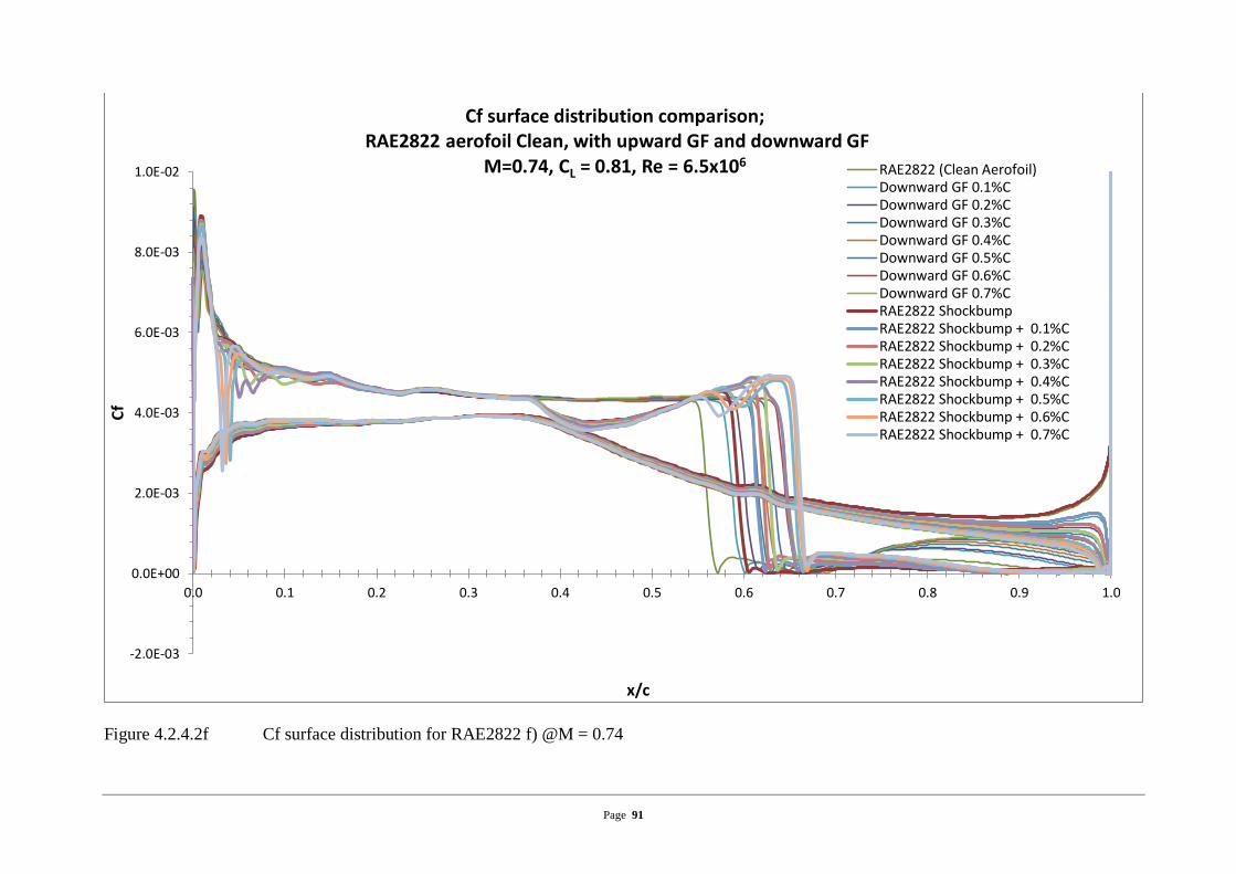


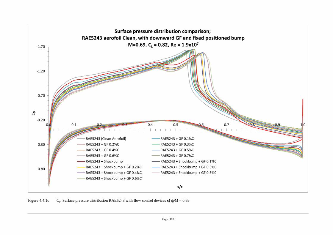


![Effect of Gurney Flap on Airfoil Lift Coefficient by Design of …jast.modares.ac.ir/article-15-20880-fa.pdf · of Gurney flap on SFYT15thick airfoil [19] Aerodynamic efficiency study](https://static.documents.pub/doc/80x56/60bd5a358e42e2274f7a1aaf/effect-of-gurney-flap-on-airfoil-lift-coefficient-by-design-of-jast-of-gurney-flap.jpg)


