Page 1
EFFECTS OF HIGH LEVELS OF STEAM ADDITION ON NOx REDUCTION IN
LAMINAR OPPOSED FLOW DIFFUSION FLAMES
by
Linda G. Blevins
Thesis submitted to the Faculty of the
Virginia Polytechnic Institute and State University
in partial fulfillment of the requirements for the degree of
MASTER OF SCIENCE
in
Mechanical Engineering
APPROVED:
U. Vandsburger
May, 1992
Blacksburg, Virginia
Page 2
ii)
v~s~
Iqqz
esl/1 C,2
Page 3
EFFECTS OF HIGH LEVELS OF STEAM ADDITION ON NOx REDUCTION IN
LAMINAR OPPOSED FLOW DIFFUSION FLAMES
by
Linda G. Blevins
Committee Chainnan: Richard J. Roby Mechanical Engineering
(ABSTRAC'O
A tlleveling off' trend in NOx emissions with high amounts of steam addition has
been observed in industrial gas turbine diffusion flame combustors. Experiments were
performed to tty to reproduce this trend in a laminar, opposed flow diffusion flame
burner. Experiments were performed with Cli4, C2H4, CO, COIH2 (1:1), and COIH2
(1:2) as fuels. Both hydrocarbon fuels and non-hydrocarbon fuels were tested to study the
contribution of the Fenimore mechanism to the "leveling off' trend. Probe sampling with
chemiluminescent analysis was used to fmd NOx concentrations; PtIPtRh thermocouples
corrected for radiation losses were used to measure flame temperatures.
The experiments reproduced the "leveling off' of NOx emissions, but a "leveling
off' of temperatures also occurred. There were no significant differences in the results
from the hydrocarbon and non-hydrocarbon fuels. The "leveling off' of NOx emissions is
attributed to the "leveling off' of temperatures in the burner. It is not necessary to invoke
the Fenimore mechanism to explain this trend. At least 55% of the NOx was eliminated
from the flames using steam injection, which implies that at least 55% of the NOx was
formed by the Zeldovich mechanism Evidence of Fenimore NO was provided by the fact
that the existence of hydrocarbon coking on the fuel nozzle encouraged NOx production
in all flames.
Page 4
ACKNOWLEDGEMENTS
I am proud to acknowledge Dr. Rick Roby for his guidance and leadership on this
project. I would especially like to thank Rick for giving me the opportunity to travel to
many technical meetings, where I made professional contacts which will be priceless
during my career. I would like to acknowledge the National Science Foundation for their
fmancial support.
I would also like to thank my parents, Martha and Lonnie Akers, and my sister,
Vicki Akers, for the love and support that they gave me. My family will be proud that I
flkept my chin up" and survived.
Thanks to the two undergraduate assistants assigned to this project, Mike Foust and
Ben Tritt. I hope that observing me hasn't frightened them away from graduate school.
Thanks to the machinists, especially Jerry Lucas and Johnny Cox. Thanks also to the
helpful employees in the instrumentation shop, Ben Poe, Frank Caldwell, Randy Smith,
and Billy Shepherd. Also, thanks to Willie Hylton for all of her help.
I want to thank the graduate students of 117 Randolph Hall, Dan Gottuk, Jim
Hunderup, Michelle Peatross, Doug Wirth, and James Reaney, for the lively conversation
and help on my project. I also appreciate the input given to me by the members of the
combustion group at Virginia Tech. I hope that the Wednesday afternoon seminars
continue to be successful in the years to come.
Finally, I thank my happy hour buddies, past and present. Happy hours kept me
sane and kept me laughing. The most important of these people were Allen Clem, Patrick
Jessee, Eric Albright, Jeff Stastny, Sandy Poliachik, Emily Scott, Tina Handlos, Jim
Hunderup, Barry Williams, and Michelle Peatross. Cheers to all of you.
iii
Page 5
LIST OF FIGURES
Page
Figure 1. Qualitative tlleveling off' ofNOx: concentrations (after Toof [6])._ 2
Figure 2. Schematic of opposed flow diffusion flame burner. 12
Figure 3. Arrangement of flow straighteners on air side of burner. 13
Figure 4. Schematic of fuel nozzle. 16
Figure 5. Schematic of steam generator setup. 17
Figure 6. Schematic of experimental setup. 20
Figure 7. Schematic of quartz sample probe. 23
Figure 8. Schematic of thermocouple mounted on sample probe. 25
Figure 9. Schematic of sampling location. 27
Figure 10. Sketch of variable voltage circuit used for calibrations. 28
Figure 11(a). NOx: concentration profiles for various amounts of steam,
CH4 as a fuel, using the clean nozzle. 37
Figure 11 (b). Temperature profiles for various amounts of steam,
CH4 as a fuel, using the clean nozzle. 37
Figure 12. NO concentration profiles for various amounts of steam,
CH4 as a fuel, using the clean nozzle. 39
Figure 13. Selected temperature profiles, CH4 as a fuel,
using the clean nozzle. 40
Figure 14(a). NOx concentration profiles for various amounts of steam,
C2H4 as a fuel, using the clean nozzle. 41
Figure 14(b). Temperature profiles for various amounts of steam, C2H4 as a fuel,
using the clean nozzle. 41
Figure 15. NO concentration proftles for various amounts of steam,
C2H4 as a fuel, using the clean nozzle. 43
iv
Page 6
Figure 16(a). NOx concentration profiles for various amounts of steam,
CO as a fuel, using the clean nozzle. 44
Figure 16(b). Temperature profiles for various amounts of steam,
CO as a fuel, using the clean nozzle. 44
Figure 17. NO concentration proftles for various amounts of steam,
CO as a fuel, using the clean nozzle. 45
Figure 18(a). NOx concentration profiles for various amounts of steam,
CO/H2 (1: 1) as a fuel, using the clean nozzle. 47
Figure 18(b). Temperature profues for various amounts of steam,
CO/H2 (1: 1) as a fuel, using the clean nozzle. 47
Figure 19. NO concentration proftles for various amounts of steam,
CO/H2 (1:1) as a fuel, using the clean nozzle. 48
Figure 20(a). NOx. concentration profiles for various amounts of steam,
CO/H2 (1:2) as a fuel, using the clean nozzle. 49
Figure 20(b). Temperature proftles for various amounts of steam,
CO/H2 (1 :2) as a fuel, using the clean nozzle. 49
Figure 21. NO concentration proftles for various amounts of steam,
CO/H2 (1:2) as a fuel, using the clean nozzle. 50
Figure 22. Peak temperatures for all fuels, using the clean nozzle. 52
Figure 23. NOx concentrations for all fuels, using the clean nozzle. 54
Figure 24. NO concentrations for all fuels, using the clean nozzle. 56
Figure 25. RNOx for all fuels, using the clean nozzle. 58
Figure 26. RNO for all fuels, using the clean nozzle. 60
Figure 27(a). NO concentration profiles for various amounts of steam,
CH4 as a fuel, using the coked nozzle. 62
v
Page 7
Figure 27 (b). Temperature profiles for various amounts of steam,
CH4 as fuel, using the coked nozzle. 62
Figure 28(a). NO concentration profiles for various amounts of steam,
C2H4 as a fuel, using the coked nozzle. 63
Figure 28(b). Temperature profiles for various amounts of steam,
C2H4 as a fuel, using the coked nozzle. 63
Figure 29(a). NO concentration profiles for various amounts of steam,
CO as a fuel, using the coked nozzle. 64
Figure 29(b). Temperature profiles for various amounts of steam,
CO as a fuel, using the coked nozzle. 64
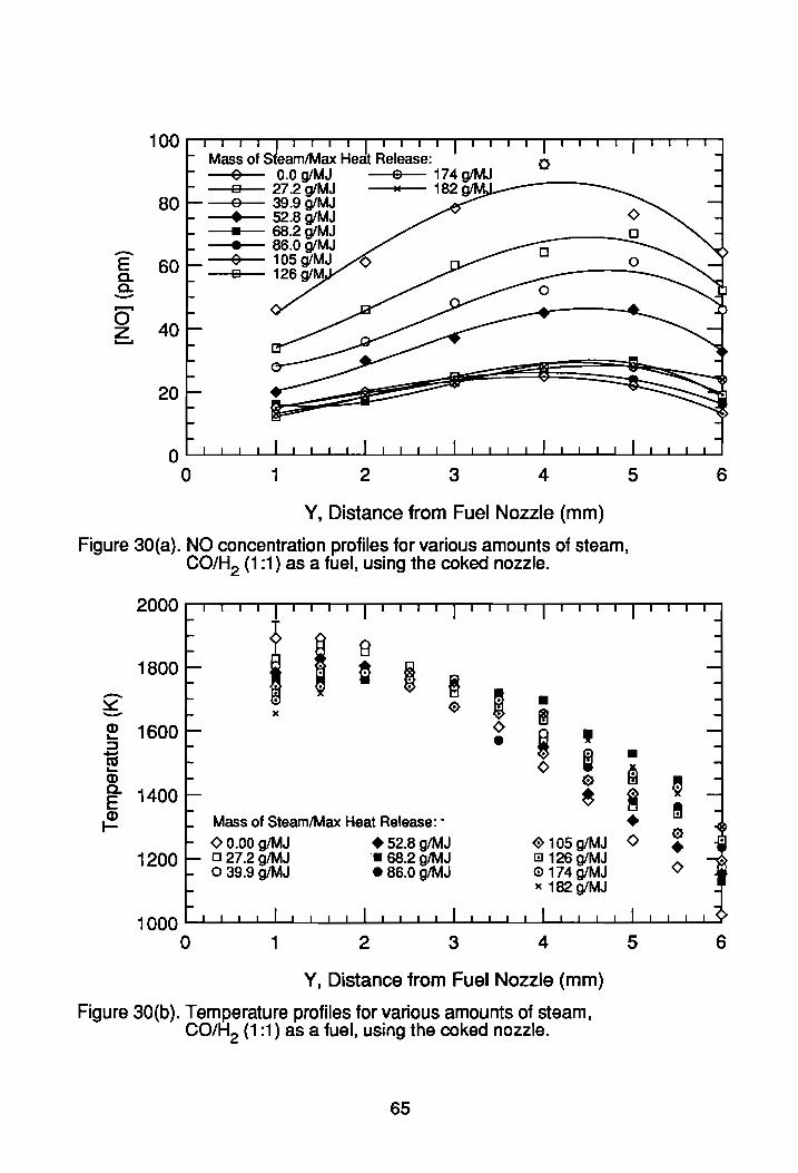
Figure 30(a). NO concentration profiles for various amounts of steam,
COIH2 (1: 1) as a fuel, using the coked nozzle. 65
Figure 30(b). Temperature profiles for various amounts of steam,
COIH2 (1: 1) as a fuel, using the coked nozzle. 65
Figure 31(a). NO concentration profiles for various amounts of steam,
COIH2 (1:2) as a fuel, using the coked nozzle. 66
Figure 31 (b). Temperature profiles for various amounts of steam,
COIH2 (1:2) as a fuel, using the coked nozzle. 66
Figure 32. NO concentration proftles, no steam, C2H4,
coked and clean nozzle. 68
Figure 33. Peak temperatures for all fuels, using the coked nozzle. 69
Figure 34(a). NO concentrations for hydrocarbon fuels,
using the coked nozzle. 72
Figure 34(b). NO concentrations for non-hydrocarbon fuels,
using the coked nozzle. 72
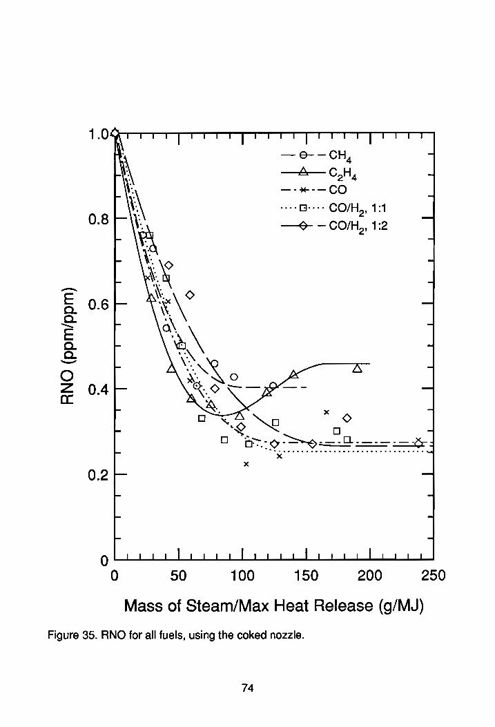
Figure 35. RNO for all fuels, using the coked nozzle. 74
vi
Page 8
Figure 36(a). Peak: temperatures for some fuels, equilibrium model. 76
Figure 36(b). Peak: temperatures for all fuels, using the clean nozzle. 76
Figure 37. Actual and equilibrium RNOx for all fuels,
using the clean nozzle. 78
Figure 38. Calibration curve for fine metering valve. 108
Figure 39. Calibration curve for variac. 109
Figure 40. Calibration curve, air, Matheson 605 tube, 550 KPa. 110
Figure 41. Calibration curve, CH4, Matheson 602 tube, 280 KPa. 111
Figure 42. Calibration curve, H2, Matheson 602 tube, 140 KPa. 112
Figure 43. Calibration curve, C2H4, Matheson 602 tube, 140 KPa. 113
Figure 44. Calibration curve, CO, Matheson 602 tube, 140 KPa. 114
Figure 45. Calibration curve, OMEGA OMNI ll-A millivolt amplifier. 115
vii
Page 9
Table 2.1.
Table 3.1.
Table 3.2.
Table 3.3.
LIST OF TABLES
Fuel Flow Rates ________________ _
Peak: Quantities and Their Locations _________ _
Comparison of NO and NOx for Clean Nozzle ______ _
Temperature Suppression _____________ _
viii
Page
30
57
61
71
Page 10
TABLE OF CONTENTS
ABsTRACT ________________________________________ __
ACKNO~DGEMENTS ______________________________ ___
LIST OFFIGURES ____________________ ___
LISTOFTABLES ___________________ _
1. ~ODUCTION ____________________________________ _
1.1. Background:..--_________________ _
1.2. NO Formation. _________________ _
1.2.1. Zeldovich NO ___________________________ _
1.2.2. Fenimore NO _______________ _
1.2.3. Fenimore NO in Premixed Flames ________ _
1.2.4. NO in Turbulent Diffusion Flames. ________ _
1.2.5. NO in Laminar Diffusion Flames _______________ _
1.2.6. Comparison of Zeldovich and Fenimore NO _____ __
1.3. Scope of the Current Work:..--___________________ _
2. EXPER~NTALAPPARATUSANDPROCEDURE ________ _
2.1. Introduction. __________________ _
2.2. Experimental Apparatus ______________ _
2.2.1. Burner Design ______________ _
2.2.2. Steam Generator ______________ _
2.3. Instrumentation:..--_____________________________ __
2.4. Experimental Procedure ______________ _
3. EXPE~NTALRESULTS _______________ ___
3.1. Introduction -----------------------------------
ix
Page
ii
iii
iv
viii
1
1
3
3
4
5
6
7
8
9
11
11
11
11
15
19
29
35
35
Page 11
3.2. Important Quantities for Comparison'-_________ _
3.3. NOx and Temperature Profiles for Hydrocarbon Fuels _____ _
3.3.1. Methane, _________________ _
3.3.2. Ethylene ________________ _
3.4. NOx and Temperature Profiles for Non-Hydrocarbon Fuels, ___ _
3.4.1. Carbon Monoxide, ______________ _
3.4.2. Carbon Monoxide with Hydrogen (1:1) _______ _
3.4.3. Carbon Monoxide with Hydrogen (1:2) _______ _
3.5. Comparison of All Fuels, _______________ _
3.5.1. Method of COmparison. _____________ _
3.5.2. Temperature _______________ _
3.5.3. NOx and NO ______________ _
3.5.4. RNOx andRNO _____________ _
3.6. Results from the Coked Nozzle ____________ _
3.6.1. NO and Temperature Profiles, __________ _
3.6.2. Comparison of All Fuels ___________ _
4. DISCUSSION __________________ _
4.1. Introduction'---_________________ _
4.2. Thermal Effect of Steam Addition'-__________ _
4.3. Comparison of Results with Past Studies _________ _
4.4. Chemical Effect of Steam Addition'---__________ _
4.5. Hints of the Existence of Fenimore NO ---------------5. SUMMARY, CONCLUSIONS, AND RECOMMENDATIONS ___ _
5.1. Summary ___________________ _
5.2. COnclusions, __________________ _
5.3. Recommendations, _________________ _
x
35
36
36
38
42
42
46
46
51
51
51
53
55
59
59
67
75
75
75
79
82
84
87
87
87
89
Page 12
REFERENCES 92
APPENDIX A: SHOP DRA WINGS OF THE BURNER 98
APPENDIX B: CALffiRATION CURVES 107
APPENDIX C: THERMOCOUPLE RADIATION CORRECrION PROGRAM_ 116
APPENDIX D: UNCERTAINTY ANALYSIS 120
VTTA 123
xi
Page 13
CHAPTER 1: INTRODUCTION
1.1. Background
Nitrogen oxides (NOx) are difficult to eliminate from industrial gas turbine
diffusion flame combustors. The constituents of NOx are nitric oxide (NO), nitrogen
dioxide (N02), and nitrous oxide (N20). Nitrogen oxides are eye and lung irritants, and
they can be fatal if inhaled in large concentrations. They may also lead to the formation
of photochemical smog and acid rain. Because of these negative effects of NOx, the
United States Environmental Protection Agency (EPA) and several state and regional
authorities restrict the amount of NOx which can be emitted by an industrial gas turbine.
Currently, the most common way of meeting requirements for NOx emissions is to inject
water or steam into the combustion chambers of the turbines [1].
Traditionally, water injection has worked very well to reduce NOx emissions to
government required levels [2,3,4]. Older combustors have been successfully retro-fitted
with water injection systems to meet emissions requirements. However, recently even
more stringent regulations on NOx emissions have been enacted or proposed in several
states, and the EPA is considering tougher national standards.
Many gas turbine operators are now finding that water or steam injection alone
does not suppress NOx concentrations to the new lower required levels [5]. In these
cases, NOx concentrations initially decline with water addition, but reach a minimum at
high amounts of water addition. Profiles of NOx concentration as a function of water
flow rate ttlevel off' at this minimum. This "leveling offt is shown qualitatively in Fig. 1.
Toof [6] presented experimental results obtained from a field test of a 25-MW
combustion turbine which showed this "leveling offt.
1
Page 14
c: o
; cu ...... +"" c: CD (.) c: o ()
x o z
Amount of Water
Figure 1. Qualitative "leveling off" at NOx concentrations (after Toot [6]).
2
Page 15
It is believed that the effects of water injection on NOx reduction are thermal in
nature. Injected water acts as a heat sink, which lowers flame temperatures. This reduces
the amount of NOx formed.
Past studies have not directly addressed the "leveling off" of NOx emissions in
industrial gas turbine diffusion flame combustors. There are several possible reasons for
the behavior of NOx emissions with high amounts of water injection. One possibility is
that the water may begin to participate chemically in the combustion reactions. Another
theory is that some of the water injected may bypass the flame front. A third potential
reason is that some of the NOx may be formed by a chemical mechanism which is
insensitive to temperature suppression. Research is needed to fmd out why high amounts
of water are ineffective at reducing NOx emissions. Investigation of this problem
requires knowledge of two of the chemical mechanisms responsible for the formation of
NOx.
1.2. NO Formation
1.2.1. Zeldovlch NO
Most of the NOx formed in industrial gas turbine combustors is formed as nitric
oxide (NO). Traditionally, the main source of NO formation in diffusion flame
combustors was believed to be the Zeldovich mechanism, which begins when an oxygen
atom (0) combines with a nitrogen molecule (N2). The Zeldovich mechanism consists of
the following reactions [7]:
O+N2=N+NO
N+D2=O+NO
3
(1.1)
(1.2)
Page 16
A third reaction thought to be important in fuel rich areas of flames follows [8]:
N+OH=H+NO (1.3)
The rate constants for the Zeldovich reactions are well known. The overall rate of NO
production from this mechanism has been shown to be a strong function of temperature.
Touchton [9], in a study of low to moderate amounts of water addition, concluded
that the effects of water were entirely thermodynamic. Touchton compared data obtained
from several gas turbine combustors incorporating water addition with predictions from
both an equilibrium chemical thermodynamics model and a chemical kinetics model. His
comparisons showed that the experimental data was best predicted by the equilibrium
calculations. However, Touchton's experiments used water addition levels below those
necessary to achieve current and proposed NOx emissions requirements. Thus, he did not
study the conditions where NOx emissions begin to "level off."
1.2.2. Fenimore NO
One possible explanation for the "leveling off' is that the water or steam
participates chemically in the combustion reactions. Miyauchi et al. [10] performed a
study of the effects of steam injection into methane-air premixed flames. In their
experiments, temperature was held constant over a range of steam injection rates.
Miyauchi found that steam does have a chemical kinetic effect on NO reduction which is
independent of the temperature suppression effect. NO concentrations were reduced with
increasing steam injection, even though temperatures were kept constant. Miyauchi
suggested that some of the NO in their premixed flames was formed by the "prompt NO"
mechanism.
4
Page 17
"Prompt NO" was frrst discovered by C.P. Fenimore [11], and hence will be called
Fenimore NO. Fenimore studied both hydrocarbon and non-hydrocarbon premixed
flames. He found that proftles of NOx concentrations versus residence time in
hydrocarbon flames could not be extrapolated to zero ppm at zero time. However, NOx
concentration in non-hydrocarbon flames did extrapolate to zero ppm at zero time.
Fenimore proposed that the "intercept Non which was predicted at zero time in the
hydrocarbon flames was formed very rapidly in the reaction zone by reactions involving
hydrocarbon fuel fragments (CHt CH2t etc.).
Fenimore NO formation is initiated when a hydrocarbon fuel fragment reacts with
a nitrogen molecule (N2). Typical Fenimore reactions follow [12]:
CH +N2=HCN+N
CH2 + N2 = HCN + NH
C2H+N2=HCN +CN
C2 +N2=CN +CN
(1.4)
(1.5)
(1.6)
(1.7)
The nitrogen species created by these reactions are rapidly converted to NO. Miyauchi
hypothesized that adding steam to their premixed flames increased hydroxyl (OH) radical
concentrations, which promoted hydrocarbon fragment oxidation. This kept the
hydrocarbon fragments from forming Fenimore NO. Thus, there was a reduction of NO
due to the chemical effect of adding the steam.
1.2.3. Fenimore NO In Premixed Flames
Many studies of Fenimore NO have been performed using premixed flames. Most
research has shown that Fenimore NO is important only in fuel rich premixed flames
5
Page 18
[11,13,14]. However, some studies have predicted that it will possibly form in fuel lean
premixed flames [15,16].
The importance of the Fenimore NO mechanism was questioned by Bowman [8]
and Sarofim and Pohl [17]. Both of these studies concluded that the rapid formation of
flame front NO could be explained by the Zeldovich mechanism if the existence of
superequilibrium oxygen atom (0) concentration was considered. However, several
researchers have found that the 0 atom concentrations would have to be unreasonably in
excess of equilibrium amounts to account for the rapid fotmation of NO formed in the
flame front [13,15,18,19].
One study which provides convincing evidence of Fenimore NO was performed by
Hayhurst and Vince [12]. They compared NO formation in premixed H2I02fN2 flames
with NO formation in the same flames with 1 % added acetylene (C2H2). They saw a
sharp increase in the flame front NO formation rate with the added hydrocarbon. This
indicated the formation of Fenimore NO. Hayhurst and others have tried to detennine
which reactions are most important in the Fenimore mechanism and to obtain expressions
for the rates of these important reactions [12,20,21,22]. However, the rates of the
Fenimore mechanism are not as well known as those of the Zeldovich mechanism.
All of these past investigations have been performed using premixed flames. The
importance of the Fenimore NO mechanism in diffusion flames has not been studied as
extensively.
1.2.4. NO in Turbulent Diffusion Flames
Results from several studies of NO formation in turbulent diffusion flames have
been published. These studies dealt with the dependence of NO fonnation on fluid
6
Page 19
mechanics quantities, such as the Froude number, the Reynolds number, and the
turbulent length scales [23,24,25,26]. Emphasis has been placed on the effects of
superequilibrium radical concentrations on NO fonnation by the Zeldovich mechanism
[27]. Results from much of the work have been distorted by probe difficulties [23,27].
Very little emphasis has been placed on studying Fenimore NO in turbulent
diffusion flames. However, Takagi et ale [25] suggested that Fenimore NO may be more
important in diffusion flames than it is in premixed flames. Takagi found that HeN
concentrations were higher for hydrocarbon diffusion flames than for hydrocarbon
premixed flames. He hypothesized that hydrocarbon fragments survive for longer periods
of time in diffusion flames than they do in premixed flames. These hydrocarbon
fragments participate in the Fenimore mechanism to produce NO. Thus, Takagi
concluded that the Fenimore mechanism may be significant in turbulent diffusion flames.
1.2.5. NO in Laminar Diffusion Flames
Turbulent diffusion flames are difficult to study experimentally and theoretically.
As a result, many researchers study laminar diffusion flames. Infonnation from
laboratory laminar diffusion flames can be used to analyze turbulent diffusion flames.
One theory which has been proposed is the "laminar flamelet theory" [28]. The laminar
flamelet theory is based upon the assumption that laminar, counterflow diffusion flames
exhibit the same scalar behavior as some turbulent diffusion flames. Laminar flamelet
theory involves studying scalar parameters of a laminar, counterflow flame, or
"flamelet." The theory involves applying these scalar parameters to a turbulence model
by predicting the probability that these flamelets will occur in a turbulent diffusion flame.
The scalars used to describe the flamelet are the mixture fraction and the instantaneous
scalar dissipation rate. Thus, the "laminar flamelet theory" uses information obtained
7
Page 20
from laminar diffusion flames to model and understand turbulent diffusion flames. Some
success has been achieved with the laminar flamelet theory by Drake et. al.[29].
Extrapolation of data from laminar diffusion flames must be done carefully, as the
laminar flamelet theory does not always apply.
Counterflow diffusion flames have been discussed thoroughly and classified by
Tsuji [30]. A laminar, opposed flow diffusion flame consists of opposing streams of fuel
and oxidizer. A flame is established on the oxidizer side of the stagnation plane where the
two streams meet The fluid mechanics and chemistry of this type of flame have been
successfully modeled [31]. The model uses potential flow assumptions and well-known
chemical mechanisms.
Counterflow diffusion flames are useful for fundamental diffusion flame chemistry
studies. Drake and Blint used modeling and experiments with laminar, opposed flow
diffusion flames to evaluate the relative importance of the Zeldovich and Fenimore NO
formation pathways in diffusion flames [32]. They concluded that more than two-thirds
of the NO formed in their diffusion flames was a result of the Fenimore NO mechanism.
Based on this conclusion, Drake and Blint suggested that the Fenimore mechanism may
also be very important in turbulent diffusion flames.
1.2.6. Comparison of ZBldovich and Fenimore NO
It is important to contrast the Zeldovich mechanism with the Fenimore mechanism.
These two mechanisms are very different. Zeldovich NO is formed in the hot post-flame
gases. The amount of Zeldovich NO is a strong function of the peak temperature and
residence time in these post-flame gases. Fenimore NO, however, is fonned very rapidly
in the flame front of hydrocarbon flames. Zeldovich NO requires only air at high
temperatures, while Fenimore NO requires the presence of fuel fragments and air.
8
Page 21
Zeldovich NO is a function of peak temperature; Fenimore NO is dependent on the
hydrocarbon content of the fuel.
The past studies of Touchton [9] and Drake and Blint [32] have addressed the
relative importance of these two NO formation mechanisms. The conclusions of these
two studies seem to contradict each other. Touchton found that water injection worked
entirely by a thermodynamic effect. He concluded that the Zeldovich mechanism was
very important in diffusion flames. However, Drake and Blint concluded that the
Fenimore mechanism was very important in their diffusion flames. Touchton would not
predict the "leveling off' of NOx emissions with increasing amounts of water; Drake and
Blint would predict that the "leveling off' is due to the existence of Fenimore NO.
Because of this conflict, additional research is needed to discover which of these studies
best predicts the behavior of diffusion flames using high amounts of water injection.
1.3. Scope of the Current Work
The overall objective of this project is to determine if water injection can be used
to meet new, lower NOx emissions requirements, or if the "leveling off' of NOx
emissions with increased water addition represents a fundamental limit for NOx
reduction by water addition. This project will involve comparison of experimental results
with chemical kinetic modeling results. This particular thesis deals with the experimental
portion of the project.
The scope of this thesis is to report on experiments which were performed to try to
reproduce the "leveling off' of NOx concentrations in diffusion flames with high levels
of steam injection in a laboratory burner. One focus of this investigation was to try to
resolve the apparent conflict between the conclusion of Touchton that the Zeldovich
mechanism is most important in turbulent diffusion flames and the conclusion of Drake
9
Page 22
and Blint that the Fenimore mechanism is most important in diffusion flames. Since
Fenimore NO will only form in hydrocarbon flames, the experiments presented in this
thesis involved injecting steam into both hydrocarbon and non-hydrocarbon diffusion
flames. Results from hydrocarbon flames and non-hydrocarbon flames with steam
addition will be compared to determine if the "leveling off' of NOx concentrations is a
result of the Fenimore NO mechanism.
10
Page 23
CHAPTER 2: EXPERIMENTAL APPARATUS AND PROCEDURE
2.1. Introduction
The opposed flow diffusion flame burner and steam generator are described in the
frrst two sections of this chapter. The next section describes the instrumentation used for
collecting data in the experiments. The final section describes the procedure followed for
performing experiments.
2.2. Experimental Apparatus
2.2. 1. Burner Design
The experimental apparatus used for this study was a laminar, opposed flow
diffusion flame burner. Detailed shop sketches and drawings of the parts of the burner are
shown in Appendix A. A schematic of the burner is shown in Fig. 2. The burner included
flow straighteners for both the fuel and air streams, and thus produced a "Type II" flame,
according to the classification by Tsuji [30]. Air flowed in the upward direction, fuel
flowed in the downward direction, and a flame was established on the air side of the
stagnation plane.
The air side of the burner consisted of a 32 em diameter sheet metal housing. The
contents of the housing were flow straightening devices separated and held in place by
pieces of 32 cm diameter poly-vinyl chloride (PVC) pipe. The outer diameter of the PVC
pipe was machined to a size slightly smaller than the inner diameter of the housing, so
that the pieces of pipe fit right into the housing. The arrangement of the flow
straighteners is shown in Fig. 3.
11
Page 24
Sample Probe with Thermocouple
To Sampling System
Air Inlet
Condensate Trap
1
Fuel +--
Inlet
Laminar Opposed Flow
+-- Diffusion Flame
+-- Pyrex Chimney
Converging
25cm
Nozzle 38 cm
+-- Steam Inlet
Air Side Housing with Flow Straighteners
Air
41cm
Inlet ---'--
Figure 2. Schematic of opposed flow diffusion flame burner.
12
Page 25
,.---- Fine Mesh Screen ro----- PVC Pipe
T 8.9 cm
,.---- Medium Mesh Screen
8.gcm
,..........-- Coarse Mesh Screen
6cm ro----- Honeycomb
1 1.6 cm
1 6.3 cm
,...--- Perforated Plate
I Air Inlets: I 32 -2.6 mm Holes
7.6cm 1/ Spaced Evenly Around PVC Pipe .~ ._ .
..JI
I· 32cm ·1
Figure 3. Arrangement of flow straighteners on air side of burner.
13
Page 26
There were four 10 mm air inlets, spaced evenly around the radius of the lower
portion of the housing. A piece of PVC pipe was placed in the bottom of the burner. A
groove was machined around the outside of the pipe, with 32 holes of 2.6 n1111 diameter
drilled in this groove. The purpose of this pipe was to distribute the four large incoming
air streams into 32 tiny evenly spaced air streams.
The air side housing also contained perforated plate, honeycomb, and coarse,
medium, and fme mesh stainless steel screens. These items were cut into circular pieces
which were 32 cm in diameter. The stainless steel perforated plate was 3 mm thick with
3.8 mm holes drilled at evenly spaced locations, while the honeycomb was 16 mm thick.
The coarse, medium, and fine screens were stretched across and attached with
screws to pieces of PVC pipe. Felt gaskets were placed between all of the pieces of PVC
pipe to seal the air side of the burner. The inner diameter of the PVC pipe matched the
inner diameter of the next piece of flow straightening equipment, the converging nozzle.
The fiberglass converging nozzle was mounted on top of the air side housing using
nuts and bolts, with a felt gasket used as a seal. The function of the converging nozzle
was to smoothly reduce the diameter of the air flow stream from 32 cm to 7 cm. The
nozzle was constructed by shaping fiberglass over a wooden mold. The mold was fonned
by glueing several poplar planks together, and then machining the poplar to the proper
shape. Finally, several coatings of polyurethane lacquer were applied to keep the surface
of the mold smooth. The fiberglass was then formed over the mold, creating a smooth
inner surface of the burner to prevent flow disturbance. The inner diameter of the
converging nozzle was matched to the next section in the air stream, the Pyrex chimney.
The chimney was made of a 25.4 cm long, Pyrex tube with a 7.5 cm outer diameter
and a 7 cm inner diameter. The Pyrex chimney sat in a groove in an aluminum flange.
14
Page 27
The flange was mounted with nuts and bolts to a flange on top of the converging nozzle.
A 13 mm diameter O-ring was used to seal the connection. The groove on the flange was
sized slightly larger than the chimney, so that the chimney could be easily removed. The
lip of the groove was tall enough to keep the chimney from falling off of the burner.
A vertical slot was cut into the side of the Pyrex chimney. The approximate
dimensions of the slot were 0.4 cm by 10.3 cm. The purpose of this slot was to provide an
opening for inserting a sample probe and a thermocouple. Due to limited glass cutting
facilities, the slot had to be cut much longer than necessary. This was the only way to
make the slot wide enough to hold the probe. In order to prevent entrainment of room air
or flow disturbance through this long slot, a piece of duct tape was placed over the
portion of the slot which was not occupied by the probe and thermocouple.
A fuel nozzle was suspended into the Pyrex chimney using a 5 mm stainless steel
tube. The fuel was delivered to the nozzle through this tube. A schematic of the fuel
nozzle is shown in Fig. 4. The fuel nozzle consisted of an uncooled stainless steel
cylinder that was 38 mm in diameter. The fuel exited the nozzle through 147 evenly
spaced, 1.6 mm diameter holes in the flat end of the cylinder. This produced 147 tiny jets
which combined to create a flat, uniform fuel supply. The cylinder was filled with 100
stainless steel beads of 2.6 mm diameter. The purpose of these beads was to create plug
flow rather than Poisselle flow exiting the fuel nozzle.
2.2.2. Steam Generator
The method of water addition used in these experiments was steam injection. A
schematic of the steam generator setup is shown in Fig. 5. The steam generator consisted
of a 5.4 em diameter cylindrical stainless steel chamber which contained a heating coil.
The lower half of the heating coil was designed to heat water; the upper half was
15
Page 28
Fuel Inlet---+
100-2.6 mm Flow Straightening Beads
y
A-
, , , '
.. .. .. .. "" .. , .. : . , :: ':: : :.' ': : : :: -:.:. :',::, ':", ... :',', : ~.. • .. :~ " .. 'f'. .. .. : : ~.. .. :." ... ::.... ...- ...... :: ................ " ... " .. ,," ........... :
.. .. f. .. " .. !"" /" •• :: .. "t, .. • !: : .. : ..... ::,," .. :: ...... :: .... :: ...... :: ..... :. : .... .' fI' , t' •• .."
: ...... " ..... ~ ...... " ..... "" "" _" '" ....... "" <I" ........... ". " ... U": ." : • :
.. .- .,. fI' ... ., .'
~. ' :', : : : ': : : : : ': : : :: ': : : : : ': : : :: ': : : : :', .. :
0000000 0000000000
0000000000 000000000000
0000000000000 0000000000000 0000000000000
0000000000000 0000000000000 000000000000 00000000000 0000000000
0000000
1<1---- 38 mm ----to!
Figure 4. Schematic of fuel nozzle.
16
147-1.6mm Holes
Page 29
Heated Steam Line
Three-Way Valve
Water Reservoir
Shutoff Valve
------,
To Burner
_--J
Condensate Trap
Drain Valve
I I I
SuperHeater
(~I File Metering Valve
I I I I I I I I I I I I I I I I I I I I I I I Heating Coil
L.....,.-----' +
Steam Generator
Figure 5. Schematic of steam generator setup_
17
1m
+
Variac
Page 30
designed to heat steam. The steam generator was equipped with a sight glass for visual
observation of the water level. The steam flow rate was controlled by using a variac to
change the amount of heat input to the steam generator. A small superheater was
mounted at the exit of the steam generator.
Distilled water was fed by gravity through 5 mm polyethylene tubing to the steam
generator. The feedwaterreservoir was a 400 ml glass beaker. The water in the reservoir
was refilled periodically to keep the water at the 200 ml level in the beaker, which
corresponded to a height of about 1 m above the point of entry into the boiler. The water
flow rate was controlled using a NUPRO fine metering valve, part number SS-SS4-A,
with a NUPRO vernier handle, part number NY-2M-K6.
The fine metering valve was calibrated using a 10 ml graduated cylinder and a
stopwatch. For each position of the vernier handle, the water flowing through the valve
was allowed to drip into the graduated cylinder. The dripping was timed using a
stopwatch, and the mass flow rate of the water was calculated. A calibration curve of
water flow rate as a function of the number of turns of the vernier handle is shown in
Appendix B.
Once the fme metering valve was calibrated, the variac could be calibrated. For
each setting of the variac, ranging from 84 V to 140 V, the position of the fme metering
valve was varied until a point was reached when the water level in the steam generator
sight glass remained constant. This assured that the water flow into the boiler matched
the steam flow out of the boiler. Thus, since the water flow rate was known, the steam
flow rate was also known. A calibration curve of steam flow rate as a function of variac
setting is shown in Appendix B.
18
Page 31
For this experiment, variac settings from 84 V to 140 V were used. The reason that
the lower limit for the variac was 84 V was that this was the lowest setting of the variac
for which steam could be generated. The upper limit was chosen because, at settings
above 140 V t the steam entering the burner contained large amounts of liquid water.
Steam was delivered to the burner in a heated, 8 mm stainless steel tube. The tube
was heated by Thermolyne silicone rubber heating tape (Fisher Scientific part number
11-463-54B). There was a condensate trap at the lowest point in the steam line. This trap
was a 4.1 cm diameter steel cylinder with a drain valve.
Steam was injected on the air side of the burner, after the flow straightening
screens but before the converging nozzle. The steam was injected in this location to avoid
condensation on the flow straightening screens. Steam flowed from the heated tube into
the center of the bottom of the air side housing. An unheated tube extended from the
bottom of the housing to the entrance of the converging nozzle. Holes were cut in the
center of the flow straightening devices so that the tube could be inserted into the burner.
Once the steam exited this unheated tube, it was entrained into the air stream. Visual
observation of the steam and air with a laser sheet proved that the steam and air were
well mixed before they contacted the flame front.
2.3. Instrumentation
A schematic of the entire experimental setup is shown in Fig. 6. Five cylinders of
breathing air were used simultaneously as the air supply for the burner. The breathing air
was mixed at an Airco facility from 02 and N 2. The specifications of this mixture were
that it contained from 19.5% to 23.5% 02, and that it contained no more than 3 ppm of
moisture. The outlets from the five cylinders were combined into one stream with
stainless steel pigtails (Airco part number PF-346) and a brass manifold (Airco part
19
Page 32
To Exhaust
Strip Chart
Recorder
M A N
+
+
Air Inlet
Fuel
Converging Noz2fe
Air FIc7N
Straighteners
Qn. densate Trap
ChemikJminescent NO/NOx Analyzer
• +
Flame Therm0-couple OutPut
Heated Steam Line
1--'
Air Inlet
I I I I I I I
~--~ ~ ~~+r----------~ o l o
Steam Thermocouple
Output
+ ~~ Meter
Figure 6. Schematic of experimental setup_
20
Water Reservoir
Page 33
number MB-346). Air flow rate was measured using a Matheson 605 series rotameter
tube. The air was delivered to the rotameter at 550 KPa. Air flow rate was controlled
using a Matheson size 9 utility metering valve on the exit of the rotameter tube. Air was
delivered to the burner in 8 mm polyethylene tubing.
The fuels burned in these experiments were methane (CH4), ethylene (C2H4) ,
carbon monoxide (CO), 50 mol% carbon monoxide with 50 mol% hydrogen (CO/H2,
1:1), and 33 mol% carbon monoxide with 67 mol% hydrogen (CO/H2, 1:2). The CH4
used was Airco Grade 1.3, which is 93% pure. The C2H4 used was Aireo Grade 2.5
which is 99.7% pure. The CO used was Aireo Grade 2.3, which is 99.3% pure. The H2
used was Airco Commercial Grade, which is 99.8% pure. As a safety precaution, small
CO detectors (Sporty's Pilot Shop #4116A) were placed around the laboratory. These
detectors are designed to change color when the concentration of CO in the air becomes
dangerous.
The two hydrocarbon fuels and three non-hydrocarbon fuels chosen for these tests
were used because Fenimore NO only forms in hydrocarbon flames. Thus, contrasting
the NO trends of hydrocarbon flames with those of non-hydrocarbon flames would
provide information about whether or not the achieved minimum NO concentrations
were a result of the Fenimore mechanism. There were two reasons that the mixtures of
CO and H2 were chosen for these tests. First, the CO/H2 (1 :2) mixture was used to create
a non-hydrocarbon fuel with the same ratio of H atoms to C atoms as the hydrocarbon
fuel of CH4. Second, the mixtures of CO and H2 were chosen to simulate the products of
coal gasification, since gasified coal is now being used as a fuel in some industrial gas
turbines [33].
21
Page 34
Methane and C2H4 were delivered at 280 KPa to a Matheson 602 series rotameter
tube. Both of these fuel flow rates were controlled with Matheson high accuracy HA-3
metering valves. Carbon monoxide was delivered at 140 KPa to a Matheson 602 series
rotameter tube, and the flow rate was controlled with a Matheson size 7 -WW metering
valve. Hydrogen was delivered at 140 KPa to a Matheson 602 series rotameter tube, and
the flow rate was controlled with a Matheson high accuracy HA-3 metering valve.
Carbon monoxide and H2 were mixed after the rotameters using a Swagelok tee. All
fuels were delivered to the burner in 5 mm polyethylene tubing.
All rotameters were calibrated using a dry gas meter (DGM) and a stopwatch. For
each setting of the rotameter, the time that it took for a known volume to pass through the
DGM was recorded. The volumetric flow rates could then be calculated. These flow rates
were corrected for standard temperature and pressure. Calibration curves for this
experiment are given in Appendix B.
An uncooled quartz probe was chosen for these experiments because conversion of
NO to N02 is less likely to happen in uncooled quartz probes than it is to happen in other
types of probes [27]. A schematic of the 3 mm uncooled quartz sample probe used in
these experiments is shown in Fig. 7. The sample was pulled through the probe into a
stainless steel section of 5 mm tubing, and then through polyethylene tubing to a
condensate trap. The condensate trap consisted of an Erlenmeyer flask with an inlet
through a hole in a rubber stopper on top and an outlet through a nipple on the side. The
flask was submerged in a bath of ice water. The sample flowed into the top of the flask,
the water condensed out, and the dry gases flowed out of the nipple.
After the sample left the condensate trap, it was introduced into a Thenno
Environmental Model 10 Chemiluminescent NO-N02-NOx analyzer. A Sargent-Welch
22
Page 35
----1 r- 0.5 mm
5.1 cm 3 mm 0.0., 1.6 mm I.D.
JoiI------10.2 cm
Figure 7. Schematic of quartz sample probe.
23
Page 36
Model 399 vacuum pump pulled the sample gases through the analyzer. The NOx
analyzer was zeroed with room air and calibrated with a certified Airco mixture of 240
parts per million (ppm) NO in N2 background. The same cylinder of span gas was used
for all calibrations. The 0-10 V output of the NOx analyzer was recorded on channell of
an Astro-Med DASH IT model MT two-channel, thermal-array strip chart recorder
(Astro-Med part number 223834220). The gain on channell of the strip chart recorder
was set at 0.2 V fdiv, with a 50 division grid. The strip chart recorder was zeroed and
spanned using the zero and full scale settings on the NOx analyzer. An uncertainty
analysis revealed that NO and NOx measurements were accurate to within 1.4%. The
uncertainty analysis is shown in Appendix D.
Uncoated Platinum-Platinum 10% Rhodium (PtJPt10%Rh, Type S) fme wire
thermocouples (OMEGA #PI0R-005-7) were used to measure flame temperature. The
thermocouple wires were 0.13 mm in diameter. Two different thermocouples were used
for these experiments. The bead diameters of the thermocouples were measured with a
photomicroscope, and were found to be 0.34 mm and 0.37 mm. An electronic ice bath,
OMEGA type MCJ-S, was used to simulate the ice bath junction.
The thermocouple was mounted on the sample probe with the bead very close to
the location of sampling. This provided a spatially consistent temperature measurement.
The thermocouple was attached to the probe by threading the 0.13 mm wires of the
thermocouple through pieces of 0.72 mm outer diameter quartz tubing. These pieces of
tubing were then attached to the quartz sample probe using Aremco alumina ceramic
putty #600. A schematic of the thermocouple and sample probe combination is shown in
Fig. 8. Since the fine thermocouple wires were not long enough to reach the cold junction
compensator, they were welded to 0.25 mm extension wires (Pt-OMEGA #SPPL-OIO,
Pt10%Rh-OMEGA #SPIORH-OIO).
24
Page 37
Thermocouple Bead
0.72 mm Quartz Tubes
3 mm Quartz Tube
O.26mmwire
+
Figure 8. Schematic of thermocouple mounted on sample probe.
25
Page 38
The sample probe and thermocouple were attached to a Unislide series A2500 X-Z
translation stage. The translation stage was mounted on an optical table. The probe and
thermocouple were inserted into the slot in the side of the chimney. Sampling was done
vertically along the stagnation plane of the flame, as shown in the location denoted by the
black square in Fig. 9. There were no differences in the trends in data collected from this
flame front location and data collected in the post flame region. The only difference in
the two sampling locations was that the NOx concentration signals were stronger from
the flame front location than from the post flame region. Thus, sampling was performed
in the flame front location.
Output from the thermocouple was amplified using an OMEGA model OMNI II-A
millivolt amplifier. Typical flame temperatures produced 0-20 m V output from the
thermocouple. The gain on the amplifier was set at five, so that its output was 0-100 m V.
The amplified thermocouple signal was recorded on channel 2 of the Astro-Med strip
chart recorder. The gain for channel 2 of the strip chart recorder was set at 2 m V /div with
a 50 division grid. The uncertainty analysis shown in Appendix D revealed that
temperature measurements were accurate to within 2.8%.
Since the millivolt amplifier was not completely linear, a calibration was made
using a variable voltage source and two voltmeters. For each input voltage to the
amplifier, the actual output voltage was recorded. A calibration curve of input voltage
versus measured output voltage was generated, and is shown in Appendix B. A sketch of
the circuit used to create the variable voltage source is shown in Fig. 10. This circuit was
also used to zero and span the strip chart recorder.
The flame temperature thermocouple readings were corrected for radiation losses
using a FORTRAN program obtained from Sandia National Laboratories [34]. The
26
Page 39
Fuel Inlet
I
Fuel Nozzle
SIDE VIEW
..........................
•
v
Denotes Sampling Location in Both Views.
•
Figure 9. Schematic of sampling location.
27
I Probe Moves Up and Down.
BOTTOM VIEW
Page 40
604 K
+
1.5 V 10 K 10 Turn Potentiometer
+
Vout
Figure 10. Sketch of variable voltage circuit used for calibrations.
28
Page 41
computer program was modified to create the data files needed for these experiments.
The program is listed in Appendix C.
A Chromel-Alumel (Type K) thermocouple probe with a stainless steel sheath
(OMEGA #KQSS-18G-12) was inserted into the steam line just before the steam entered
the burner. An OMEGA type MCJ-K cold junction compensator was used to simulate the
ice bath .. Output from the thermocouple was visually read from a digital voltmeter. The
temperature of the steam before it entered the unheated section of tubing was typically in
the range of 378 K to 398 K.
2.4. Experimental Procedure
Different flow rates were used for the five different fuels. These flow rates varied,
depending on the stability limits of the fuel in the opposed flow burner. The only
exception to this was C2H4. The C2H4 flow rate was limited by excessive soot
formation. The different fuel flow rates are shown in Table 2.1.
In past studies, a common way to operate opposed flow burners was to inject N2
on the fuel side of the burner [32, 35]. This created higher fuel velocities, which caused
the flames to stabilize far away from the fuel nozzle. This made the flames more
adiabatic. Thus, injecting N2 with the fuel produced more stable flames by eliminating
the heat losses to the fuel nozzle. However, N2 was not injected with the fuel in the
experiments presented in this thesis so that the N2 chemistry of the fuel-air diffusion
flame would not be disturbed. Thus, the flames in this study stabilized close to the
stainless steel fuel nozzle, and were often difficult to stabilize.
The air flow rate was kept constant at 94 sVmin or 121 glmin for all experiments.
This was to keep the radial strain rate constant. The average velocity of the air in the
29
Page 42
Fuel
C2H4
co
COIH2 (1:1)
CO
H2
CO/H2 (1:2)
CO
H2
Volumetric Flow Rate
(s1/min)
0.77
0.29
1.13
0.80
0.80
0.40
0.80
Table 2.1. Fuel Flow Rates
Mass Flow Rate
(g/min)
0.55
0.36
1.40
1.0
0.07
0.50
0.07
30
Lower Heating Value
(MJ/kg)
50
50
10.1
10.1
120
10.1
120
Maximum Heat Release Rate(KW)
0.46
0.30
0.24
0.31
0.17
0.14
0.22
0.08
0.14
Page 43
chimney was 0.5 mls. The Reynolds number of the air stream was 2200. The radial strain
rate was 13 s-l. The strain rate, "a," was calculated assuming axisymmetric plug flow
[36]. The following relationship was used:
a=U/2R (2.1)
In this equation, U is the air stream velocity, and R is the radius of the fuel nozzle.
The overall steam flow rates used in these experiments ranged from 2 g/min to 12
g/min. Steam flow measurements were estimated to be accurate to within 1 g/min. As
mentioned previously, the air and steam were well mixed when they contacted the flame
front. Since the fuel nozzle occupied 30% of the area of the chimney, the assumption was
made that 30% of the steam contacted the flame front. Using this assumption, the
corrected steam flow rates were 0.6 g/min to 3.6 g/min.
The fIrSt step in preparing to collect data was to zero and span the Astro-Med strip
chart recorder. Next, the NOx analyzer was calibrated. For these experiments, the strip
chart recorder was operated at 1 mm/s. The flame was ignited and allowed to bum for a
few minutes so that the burner could get heated up and the flame could reach steady state.
Care was taken to make sure the sample probe was positioned over the center hole at the
exit of the fuel nozzle.
During data collection, temperature was measured at 0.5 nun increments through
the flame; NO and NOx were measured in 1 nun increments. An error analysis shown in
Appendix D indicated that the distance from the fuel nozzle was known to within 0.5
mtn. The first step in collecting data was to move the sample probe up into the flame
until it was touching the fuel nozzle. This location corresponded to Y = 0 mm. Both
flame temperature and NO concentration were recorded on the strip chart recorder. The
31
Page 44
time response of the thennocouple was much quicker than the time response of the NO
analyzer. Thus, data collection involved waiting for the NO reading to reach a steady
value. Visual monitoring of the strip chart recorder was used to determine when the NO
reading reached steady state. Once the NO reading was taken, the analyzer was switched
to NOxmode.
After a clear NOx reading was obtained, the probe was translated down to Y = 0.5
mm. In this location, only a temperature reading was made. Then, the probe was
translated down to Y = 1 mm. Temperature, NO, and NOx were recorded. This procedure
continued until sampling was completed at 4 mm or 5 mm away from the fuel nozzle.
Experiments perfonned by translating the probe up from below the flame instead of
down from the burner showed no difference in measurements to within experimental
accuracy.
Once data had been obtained for the flame without steam injection, the steam
generator was turned on. The variac was set at 84 V; the vernier valve handle on the
water supply was set at 9.7 turns. The experiment was allowed to run for a few minutes to
reach steady state. Then, the condensate trap was drained and a stopwatch was set.
The sampling procedure described for the flame with no steam injection was
repeated for the flame with steam injection. The steam thermocouple voltage was
manually recorded. When sampling was completed, the steam trap was drained and the
stopwatch was turned off. The average condensate flow rate for the run was then
calculated and subtracted from the overall steam flow rate to obtain a net steam flow rate.
This procedure was repeated for eight or nine different steam injection amounts.
The NOx analyzer was recalibrated between each run. If the NOx analyzer calibration
32
Page 45
was off by more than 2% of the maximum reading, the data was taken again. The
approximate time that it took to run one experiment was five hours.
Each fuel was tested twice. After all of the first experiments were perfonned once,
disassembly of the fuel nozzle revealed heavy coking on the stainless steel beads inside
the nozzle. This coking was caused by pyrolysis of fuel in the hot stainless steel nozzle.
Several CH4 and C2H4 flames had been burned in the nozzle before testing began. As a
result, partially pyrolyzed hydrocarbon fragments were deposited in the nozzle.
Therefore, hydrocarbon fragments were available to form Fenimore NO during all of the
frrst experiments, including the ones performed with non-hydrocarbon fuels.
Once this coking was discovered, all the tests were run for a second time. The fuel
nozzle and beads were thoroughly cleaned in an ultrasonic cleaner before each
subsequent test. This cleaning affected the outcomes of the experiments. The differences
in the results from the coked nozzle and the clean nozzle will be discussed in the next
section of this paper.
One difference in the flI'St set of experiments performed and the last set of
experiments performed was that total NOx measurements could not be determined during
the early experiments. This was because of the existence of certain species in the flame
front which cause the catalyst in the N02 to NO converter to reduce both N02 and NO
back to N2 [16,37]. Some researchers have been able to avoid this problem by operating
their N02 to NO converter at 4001 C rather than the usual 600l C [16].
An interesting problem occurred when testing the pure CO flames in the clean
nozzle. The CO flame was very unstable, and it continually blew off. Introduction of a
very small steam flow rate to the air side of the burner stabilized the flame. The OH
radicals introduced by the steam were enough to keep the CO steadily burning in air.
33
Page 46
Experiments were performed as described above, but baseline data for the flame with no
steam injection could not be obtained.
A probe effect was observed during data collection. As the probe was traversed
down through the flame, a point was reached when the flame stabilized on the probe, and
was actually pulled down into the probe. This distorted the data by creating a second
peak: in the NO and NOx concentration profiles. Although the second peak existed for all
flames in this study, the second peak: was not considered to be an actual data point
because the shape of the flame was distorted by the probe. Thus, although it is important
to know that it exists, the second peak: will not be presented in this thesis as actual data.
34
Page 47
CHAPTER 3: EXPERIMENTAL RESULTS
3.1. Introduction
The first section of this chapter describes the important quantities which are used
to compare the results from the different fuels. Graphs of NOx concentration and
temperature as functions of the distance from the fuel nozzle are presented for the
hydrocarbon fuels and non-hydrocarbon fuels in the following two sections. The next
section compares the results from all of the fuels by presenting graphs of peak
temperature, peak NOx concentration, and the percentage of NOx removed (RNOx) as
functions of the amount of steam added. Results from the flames burned in the coked
nozzle are shown in the final section of this chapter.
3.2. Important Quantities for Comparison of Results
Traditionally, for steam injection studies, NO concentrations have been plotted as
functions of the ratio of the mass flow rate of steam to the mass flow rate of fuel. In this
study, NO concentrations and temperatures are plotted as functions of the ratio of the
mass flow rate of steam to the maximum heat release rate of the fuel. This is a more
meaningful quantity for comparing fuels with different heating values. The maximum
heat release rate is the product of the fuel flow rate and its lower heating value. Heating
values and maximum heat release rates for the flames used in these experiments are
shown in Table 2.1. The maximum heat release rate is proportional to the peak
temperature that can exist in a flame. Since steam injection studies deal with suppressing
this peak temperature by different amounts, the ratio of the mass flow rate of steam to the
maximum heat release rate of the fuel is an important quantity for comparison.
35
Page 48
It is more important to study the trends in NOx concentrations than it is to study
the trends in NO concentrations. This is because past studies showed that some of the NO
in the sample is converted to N02 in the probe [38]. Since N02 will not fonn at the high
temperatures that exist in the flames, any N02 in the sample is fonned from NO in the
probe [37]. If this is the case, then total NOx concentration measurements will represent
the original amount of NO in the sample. Total NOx data will be emphasized for the
clean nozzle, but NO data will be considered for the coked nozzle since total NOx
measurements were not made with the coked nozzle.
A useful way to look at NOx with steam injection is to divide the NOx
concentration with steam injection by the NOx concentration measured in the same flame
with no steam injection. This gives a normalized quantity which ranges from zero to one.
This quantity is called RNOx, and it represents the percentage of the original NOx which
remains in the flame with a particular steam injection amount This study will use both
RNOx and RNO for comparisons.
One error bar is shown on each graph which displays NO concentrations, NOx
concentrations, or temperatures in this section. In some cases, the error bar is not visible
on the graph. This is because the error bar is smaller than the symbol used to plot the
data. Thus, where error bars are not visible, the symbol size approximates the error.
3.3. NOx and Temperature Profiles for Hydrocarbon Fuels
3.3.1. Methane
Figure 11(a) and Fig. 11(b) show NOx concentrations and temperatures,
respectively, as a function of distance from the fuel nozzle for CH4. Concentrations of
NOx are initially in the range of 70 ppm, and are reduced to the range of 40 ppm at large
36
Page 49
-E Q. Q. -x o z ........
80
60
40
20 Mass of Steam/Max Heat Release: o 19.0 g/MJ • 38.2 g/MJ o 28.3 g/MJ • 49.7 g/MJ
-.e- 63.1 g/MJ
-~o- 77.9 g/MJ -80- 94.0 g/MJ -~O-125.0 g/MJ
o~~~~~~~~~~~~~~~~~~~~~~~
o 1 2 3 4 5
Y, Distance from Fuel Nozzle (mm)
Figure 11 (a). NOx concentration profiles for various amounts of steam, CH4 as a fuel, using the clean nozzle.
1800
-~ -~ 1600 ::::I is .... Q)
~ 1400 Q)
~ . 1200 ·
1000 0
i ~ a ij 9 0
~ a $ ~ ~ <:>
Mass of SteamlMax Heat Release:
<> 0.00 glMJ + 38.2gIMJ D 19.0 g/MJ .49.7 glMJ 028.3 g/MJ .63.1 g/MJ
1 2 3
i • 0 , 0 $ EI Q
$ ~
~77.9 g/MJ El94.0 glMJ 0125 g/MJ
4
Y, Distance from Fuel Nozzle (mm)
Figure 11 (b). Temperature profiles for various amounts of steam, CH4 as a fuel, using the clean nozzle.
37
<>
5
6
6
Page 50
amounts of steam injection. With no steam injection, the temperature peaks at 1722 K,
and is reduced to 1570 K. Thus, for this CH4 flame and for most of the other flames in
this study, steam injection suppresses flame temperatures.
Profiles of NO concentration as a function of the distance from the fuel nozzle for
the CH4 flame are shown in Fig. 12. Concentrations of NO are initially in the range of 70
ppm, and are reduced to the range of 20 ppm with large amounts of steam. The NO
concentration curves have the same shapes as the NOx concentration curves for the clean
nozzle shown in Fig. 11(a). The only differences in the two sets of proflles are the
absolute magnitudes of the concentrations.
Figure 13 provides a closer look at temperature proflles for four amounts of steam
addition into the CH4 flame. With no steam injection, temperature peaks at a distance of
2.3 mm from the fuel nozzle. The proflle for the steam amount of 28.3 g/MJ peaks at a
distance of 2.1 mm from the fuel nozzle. The profile for the steam amount of 63.1 g/MJ
peaks at a distance of 1.9 mm from the fuel nozzle. The profIle for the steam amount of
125 g/MJ peaks at a distance of 1.7 rom from the fuel nozzle. This data shows that as the
amount of steam injected increases, the peak temperature for CH4 moves 0.5 rom closer
to the fuel nozzle. This verifies the visual observation that the CH4 flame moved
physically closer to the fuel nozzle as steam injection increased. Methane flames were the
only flames in this study which noticeably moved in space.
3.3.2. Ethylene
Total NOx concentration profIles and temperature profiles for the C2H4 flame are
shown in Fig. 14(a) and Fig. 14(b), respectively. Concentrations of NOx are initially in
the range of 100 ppm, and are reduced to the range of 30 ppm. The peak temperature
with no steam injection is 1591 K, and temperatures are suppressed as low as 1489 K.
38
Page 51
....... o z ..........
80
60
40
20
Mass of Steam/Max Heat Release: o 0.0 g/MJ • 38.2 g/MJ o 19.0 g/MJ • 49.7 g/MJ o 28.3 g/MJ • 63.1 g/MJ
o 77.9 g/MJ 8 94.0 g/MJ o 125.0 g/MJ
o~--~~--~~~~~~~~~--~~--~---
Figure 12.
o 1 2 3 4 5
Y, Distance from Fuel Nozzle (mm) NO concentration profiles for varying amounts of steam, CH4 as a fuel, using the clean nozzle.
39
6
Page 52
Mass of Steam/Max Heat Release: V' 0.0 g/MJ
.... G· ... 28.3 g/MJ - e- - 63.1 g/MJ --~--125g/MJ
1800
..--... ~ 1600 ........, Q) ~
:::J +-' «S ~
Q) 0..
" E Q) 1400 ~ I- " '<>
1200
1000~~~~~~~~~~~~~~~
o 1 2 3 4 5
Y, Distance from Fuel Nozzle (mm) Figure 13. Selected temperature profiles, CH4 as a fuel,
using the clean nozzle.
40
6
Page 53
180
160 Mass of Steam/Max Heat Release:
o 0.0 g/MJ • 54.9 g/MJ e 110 g/MJ
140 o 30.7 g/MJ • 69.3 g/MJ a 42.0 g/MJ • 87.7 g/MJ
o 130 g/MJ e 172 g/MJ
- 120 E 0- 100 0---x 80 0 z ........ 60
40
20
0 0 1 2 3 4 5
V, Distance from Fuel Nozzle (mm)
Figure 14(a). NOx concentration profiles for various amounts of steam, C2H4 as a fuel, using the clean nozzle.
2000 Mass of Steam/Max Heat Release:
1800 <> 0.00 g/MJ +S4.9g/MJ ~ 110 g/MJ 030.7 g/MJ .69.3 g/MJ [!J 130 g/MJ 042.0 g/MJ .87.7 g/MJ (;) 172 glMJ -~
j - 1600 <> Q)
S '- I ::J j ca e
-'- G Q) 1400 0 [3
! 0- m ~ E 1H e Q) 1H t- 1200
1000
0 1 2 3 4
V, Distance from Fuel Nozzle (mm)
Figure 14(b). Temperature profiles for various amounts of steam, C2H4 as a fuel, using the clean nozzle.
41
5
6
6
Page 54
Figure 15 shows NO profiles for the C2R4 flame. Concentrations of NO are
initially in the range of 80 ppm, and are reduced to the range of 10 ppm. These NO
profiles exhibit the same basic behavior as the NOx profiles for the clean nozzle shown
in Fig. 14(a).
3.4. NOx and Temperature Profiles for Non-Hydrocarbon Fuels
3.4. 1. Carbon Monoxide
The CO flame with no steam injection could not be stabilized. Thus, data was not
obtained for the dry CO flame. Adding a small amount of steam, which corresponded to
43.1 g/MJ, helped with stability. The purpose of adding a small amount of steam was to
introduce OR radicals to stabilize the flame.
Total NOx profiles and temperature profiles for CO flames are shown in Fig. 16(a)
and Fig. 16(b), respectively. Concentrations of NOx are initially in the range of 10 ppm,
and are reduced to the range of 4 ppm. Temperature for this CO flame initially decreases
but eventually begins to increase with increasing amounts of steam. With the lowest
steam amount, the temperature profile peaks at 1065 K. The temperature reaches a
minimum of 1023 K, but actually increases to 1086 K at the highest amount of steam
addition. Thus, the temperatures of the CO flames decrease with moderate steam
addition, and then increase with high amounts of steam addition.
Nitric oxide profiles for the CO flame are shown in Fig. 17. Concentrations of NO
are initially in the range of 10 ppm, and are reduced to the range of 3 ppm. These NO
profiles exhibit the same basic behavior as the NOx profiles of Fig. 16(a).
42
Page 55
180
Mass of Steam/Max Heat Release:
160 ~ 0.0 g/MJ 8 30.7 g/MJ e 42.0 g/MJ • 54.9 g/MJ
140 • 69.3 g/MJ • 87.7 g/MJ $ 110 g/MJ 8 130 g/MJ
120 9 172 g/MJ
..--..... E 100 a. a.
""'-'" r---I
0 80 Z .........
60
40
20
o~~~~~~~~~~~~~~~~~~~
Figure 15.
o 1 2 3 4 5
Y, Distance from Fuel Nozzle (mm) NO concentration profiles with various amounts of steam, C2H4 as a fuel, using the clean nozzle.
43
6
Page 56
15 Mass of Steam/Max Heat Release:
~ 43.1 glMJ B 57.7 glMJ e 76.4 glMJ • 98.0 glMJ - 10 • 126 g/MJ
E • 167 glMJ C- O 181 g/MJ c. 0 240 glMJ -x 0 z .......
5
o~~~~~~~~~--~~~~~~--~~~--~---
o 1 2 3 4 5
Y, Distance from Fuel Nozzle (mm)
Figure 16(a). NOx concentration profiles for various amounts of steam, CO as a fuel, using the clean nozzle.
1300
-~ -l!? 1100 ::J
! CD c. E Q) I-
900
700
Mass of Steam/Max Heat Release:
<> 43.1 g/MJ • 98.0 g/MJ 057.7 g/MJ • 126 glMJ o 76.4 g/MJ • 167 g/MJ
~ ~ a e 8 ~
I @ @ , • t , til • •
! ,
~ 181 g/MJ [!J 240 g/MJ
I @
• <>
6
500~~~~~~~~~~~~~~~~~~~~~~
o 1 2 3 4
Y, Distance from Fuel Nozzle (mm)
Figure 16(b). Temperature profiles for various amounts of steam, CO as a fuel, using the clean nozzle.
44
5 6
Page 57
4
~3 E a. a. '-'"
o z .......... 2
1
Mass of Steam/Max Heat Release: o 43.1 g/MJ o 57.7 g/MJ o 76.4 g/MJ • 98.0 g/MJ • 126 g/MJ • 167 g/MJ ~ 181 g/MJ 8 240 g/MJ
o~~~~~~~~~~~~~~~~~~~~
Figure 17.
o 1 2 3 4 5
Y, Distance from Fuel Nozzle (mm) NO concentration profiles for various amounts of steam, CO as a fuel, using the clean nozzle.
45
6
Page 58
3.4.2. Carbon Monoxide with Hydrogen (1:1)
Total NOx concentration proflles and temperature profiles for CO/H2 (1: 1) are
shown in Fig. 18(a) and Fig. 18(b), respectively. Concentrations of NOx are initially in
the range of 40 ppm, and they are reduced to the range of 10 ppm. The peak temperature
with no steam injection is 1855 K, and it is suppressed as low as 1834 K. This is a very
small amount of temperature suppression. Within experimental accuracy limits, the peak
temperature in the CO/H2 (1:1) flame remains constant.
Nitric oxide concentration profiles for the CO/H2 (1:1) flame are shown in Fig. 19.
Concentrations of NO are initially in the range of 40 ppm, and they are reduced to the
range of 10 ppm. These NO profiles have the same basic shapes as the NOx profiles
shown in Fig. 18(a).
3.4.3. Carbon Monoxide with Hydrogen (1 :2)
Proflles of NOx concentration and temperature are shown for the CO/H2 (1:2)
flame in Fig. 20(a) and Fig. 20(b), respectively. Concentrations of NOx are initially in the
range of 8 ppm, and they are reduced to the range of 1 ppm. The peak temperature for no
steam injection is 1618 K, and it is suppressed to 1345 K.
Nitric oxide proflles for the CO/H2 (1:2) flame are shown in Fig. 21. NO
concentrations are initially in the range of 4 ppm, and are reduced to the range of 0.1
ppm. The NO proflles exhibit the same basic shapes as the NOx profiles shown in Fig.
20(a).
46
Page 59
40
-E 30 a. a. --x ~ 20 .........
10
0 0 1 2 3 4 5
Y, Distance from Fuel Nozzle (mm)
Figure 18(a). NOx concentration profiles for various amounts of steam, CO/H2 (1:1) as a fuel, using the clean nozzle.
2000
1800 M
a § ~ e 0
- 0 I G.1 ~ - i ~ Q) 1600 0 [J
~ ~
::J 1\1 0 ~ ~ • Q) a. 1400 0 E Q) [J .....
Mass of Steam/Max Heat Release: 1200 00.00 g/MJ +59.8 g/MJ
[J 32.1 g/MJ .74.7 g/MJ o 45.5g/MJ .95.4 g/MJ
1000 0 1 2 3 4
Y, Distance from Fuel Nozzle (mm)
Figure 18(b). Temperature profiles for various amounts of steam, CO/H2 (1 :1) as a fuel, using the clean nozzle.
47
5
6
6
Page 60
40
~ 30 E a. a. ............
o z ........ 20
10
Mass of Steam/Max Heat Release: 0.0 g/MJ • 59.8 g/MJ $
-+-+-- 32.1 g/MJ • 74.7 g/MJ 0 -+-+--- 45.5 g/MJ • 95.4 g/MJ 9
114 g/MJ 136 g/MJ 185 g/MJ
o~~~~~~~~~~~~~~~~~~~~
Figure 19.
o 1 2 3 4 5
Y, Distance from Fuel Nozzle (mm) NO concentration profiles for various amounts of steam, CO/H2 (1 :1) as a fuel, using the clean nozzle.
48
6
Page 61
-E a. a. --x o z --
8
6-
4
2
0 0
Mass of Steam/Max Heat Release: o 0.0 g/MJ e 126 g/MJ o 43.1 g/MJ e 155 g/MJ o 58.4 g/MJ • 77.2 g/MJ • 97.7 g/MJ
o 181 g/MJ o 242 g/MJ
1 2 3 4 5
V, Distance from Fuel Nozzle (mm)
Figure 20(a). NOx concentration profiles for varying amounts of steam, CO/H2 (1 :2), using the clean nozzle.
2000 Mass of Steam/Max Heat Release:
1800 <> 0.00 g/MJ +77.2g/MJ ~ 155 g/MJ 043.1 g/MJ .97.7 g/MJ [3 181 g/MJ 058.4 g/MJ e126 g/MJ 0242g/MJ -~
~ - 1600 CD ft a ... ::l 0 1ti + m + 0 ...
1400 e e m D CD • • g c.
~ 8 ~ 0 E ~
[3 0 CD ~ e a r-1200 ~ [3
G i 8
~
1000 t;J • D
0 1 2 3 4 5
V, Distance from Fuel Nozzle (mm)
Figure 20(b). Temperature profiles for various amounts of steam, CO/H2 (1 :2) as a fuel, using the clean nozzle.
49
6
6
Page 62
.............
E c.. c. ...........
,....... 0 Z ..........
Figure 21.
Mass of Steam/Max Heat Release: o 0.0 g/MJ o 43.1 g/MJ o 58.4 g/MJ • 77.2 g/MJ
4 • 97.7 g/MJ • 126 g/MJ $ 155 g/MJ D 181 g/MJ o 242 g/MJ
3
2 0 0 0
1
o~~~~~~~~~~~~~~~~~~~~
o 1 2 3 4 5
Y, Distance from Fuel Nozzle (mm) NO concentration profiles with various amounts of steam, CO/H2 (1 :2), using the clean nozzle.
50
6
Page 63
3.5. Comparison of All Fuels
3.5.1. Method of Comparison
Because the flames can move physically in space, an NOx measurement at 1 mm
from the fuel nozzle with no steam injection may not compare with an NOx measurement
at 1 mm from the fuel nozzle with high steam injection. These may be physically two
different points in the flame. To compensate for this ambiguity, for each steam amount in
a particular flame, the peak NOx concentration, no matter how far it is located from the
nozzle, is chosen for comparison with other peak NOx concentrations. Likewise, for each
steam flow rate, the peak temperatures are chosen for comparison.
3.5.2. Temperature
Graphs of temperature versus the amount of steam addition are presented in this
section. In general, temperatures are not suppressed uniformly in these opposed flow
diffusion flames with increasing steam addition. Most of the graphs exhibit a "leveling
off' trend. For this analysis, the uleveling off' value represents an average of the data
points after the point is reached where temperatures no longer decrease.
Peak temperatures as a function of the amount of steam for each fuel are shown in
Fig. 22. The temperature curves "level ofr' for CH4 and C2H4. Temperature in the CH4
flame starts at 1722 K and "levels ofr' at 1570 K with a steam amount of about 110 g/MJ.
Temperature in the C2H4 flame starts at 1618 K and "levels ofr' at 1497 K with a steam
amount of about 150 g/MJ. As mentioned previously, temperature in the CO flame
decreases to a minimum and then increases again. Temperature in the CO flame starts at
1065 K, decreases to 1023 K at the steam amount of 1 ()() g/MJ, and then increases to a
maximum of 1086 K at a steam injection amount of about 250 g/MJ. In the CO/H2 (1: 1)
51
Page 64
1800
...-... ~ "-'
Q) 1600 "-::J ....... as "-CD a.
, , 0 '- 0 "·0 0 """" '. ---flllt---"c:t"Qs"OD .. .......: )4-:-0.
'. -"_.. r'\ . '. . 0 o· - .. - .. ..:::.! .. - .. -
x'. E ". X Q)
1400 I-~ as Q)
0...
- 'V'- - CO/H2, 1:1
-O--CH4 --&-- C
2H4
x '. , ... )C ••••••• '
1200 ..... )( . . .. CO/H
2, 1:2
---to-+- - CO
1000
o 50 100 150 200 250
Mass of Steam/Max Heat Release (g/MJ)
Figure 22. Peak temperatures for all fuels, using the clean nozzle.
52
Page 65
flame, temperatures are "level" over the entire range of steam amounts. Temperature in
this CO/H2 (1:1) flame starts at 1855 K and remains essentially constant, dropping only
to 1834 K. Temperature in the CO/H2 (1:2) flame decreases to a minimum and then
increases again. This temperature in the CO/H2 (1:2) flame starts at 1618 K, drops to
1345 K at a steam amount of 150 g/MJ, and increases again to 1447 K at a steam amount
of about 250 g/MJ. All temperatures "level off' at a steam amount of 100-150 g/MJ.
3.5.3. NOx and NO
The "leveling off' of NOx concentrations observed in gas turbine combustors was
reproduced in both the hydrocarbon and non-hydrocarbon laboratory diffusion flames.
Graphs of NOx concentrations and NO concentrations versus the amount of steam
injected are presented in this section. All of these graphs exhibit the "leveling off' trend.
For this analysis, the ttleveling off' value represents an average of the data points after
the point is reached where NOx or NO concentrations no longer decrease.
Figure 23 shows total NOx concenttation as a function of the amount of steam for
each fuel. Total NOx concentrations in the CH4 flame start at 92 ppm and "level off' at
41 ppm with a steam amount of about 110 g/MJ. Total NOx concentrations in the C2H4
flame stan at 98 ppm and "level off' at 30 ppm with a steam amount of about 150 g/MJ.
Total NOx concentrations in the CO flame start at 11 ppm and "level off' at 4.3 ppm with
a steam amount of about 130 g/MJ. Total NOx concentrations in the CO/H2 (1:1) flame
start at 46 ppm and "level off' at 15 ppm with a steam amount of about 120 g/MJ. Total
NOx concentrations in the CO/H2 (1:2) flame start at 7.9 ppm and "level off' at 1.6 ppm
with a steam amount of about 150 g/MJ. All of these NOx concentration curves "level
off' at steam amounts of 100-150 g/MJ. This graph shows that total NOx concentrations
53
Page 66
A C2H4 -e--CH4 .... [3 .... CO/H
2, 1 :1
80 --*"--CO ----fO~ - CO/H
2, 1 :2
............ ~
60 ..... "0 -E c.. c.. ~
,......., x
0 40 Z ....... "0 0
D'·.
20 0-0 -0--. 0 -CJ" ..................... .
o~~~~~~~~~~~~~~~~--~
o 50 100 150 200 250
Mass of Steam/Max Heat Release (g/MJ)
Figure 23. NOx concentrations for all fuels, using the clean nozzle.
54
Page 67
for the hydrocarbon fuels are higher than the total NOx concentrations for the non
hydrocarbon fuels.
Figure 24 shows NO concentration measurements as a function of steam amount.
Comparison of Fig. 24 with Fig. 23 shows that there is a large amount of N02 formed in
the C2H4 flame. The difference between the amount of NOx and the amount of NO
measured at the "leveling off' point of the C2H4 flame is 22 ppm, whereas this
difference is 12 ppm, 4 ppm, 2 ppm, and 1.5 ppm, for CH4, CO, CO/H2 (1:1), and
COIH2 (1:2), respectively. The excessive amount of N02 in the C2H4 flame was most
likely formed in the sample probe. The existence of hydrocarbons in the probe promote
NO to N02 conversion. Hori showed that C2H4 promotes this conversion more readily
than does CH4 [39].
Table 3.1 summarizes the peak NOx concentration and the peak temperature for
each flame. The locations of these peak quantities are also shown. This data shows that
the NOx concentration peaks on the air side of the location of the peak temperature for all
fuels.
3.5.4. RNOx and RNO
RNOx represents the percentage of the original NOx which is removed with steam
addition. Graphs of RNOx versus the amount of steam added are presented in this
section. Comparison of RNOx for different fuels shows the effectiveness of steam for
eliminating NOx in different types of flames.
Figure 25 shows RNOx as a function of the amount of steam. For all fuels, RNOx
"levels off." For the CH4 flame, RNOx "levels off' at 0.46 with a steam amount of 125
g/MJ. For the C2H4 flame, RNOx "levels off' at 0.31 with a steam amount of about 150
55
Page 68
.. E c.. c.. "-" r--"'I
80
~ 40 ........
20
A C2H4 -e--CH4 •... [3_ ••• CO/H
2, 1:1
---M---CO ---fO-+- - CO/H2 , 1:2
~o ---0--
OLL~L£~~~~~~~~~~~~~~
o 50 100 150 200 250
Mass of Steam/Max Heat Release (g/MJ)
Figure 24. NO concentrations for all fuels, using the clean nozzle.
56
Page 69
Table 3.1. Peak Quantities and Their Locations
PeakNOx Y, Distance Peak Y, Distance Concentration from Temperature from
Fuel (ppm) Nozzle (mm) (K) Nozzle (mm)
92 2.5 1722 2.0
C2,H4 98 2.5 1618 1.5
CO 11 4.0 1065 1.5
CO/H2 (1:1) 46 3.0 1855 2.0
COIH2 (1:2) 7.9 4.0 1618 1.5
57
Page 70
0.8
x o z 0.4 a:
0.2
. \ 'x \ . \ , \ • \
t
\x \ , \ ,
\
-e--CH4 A C2H4
--*--CO .... [3- •.. CO/H
2, 1:1
----E:O-+- - CO/H2, 1:2
o~~~~~~~~~~~~~~~~~~
o 50 100 150 200 250
Mass of Steam/Max Heat Release (g/MJ)
Figure 25. RNOx for all fuels, using the clean nozzle.
58
Page 71
g/MJ. Since the dry CO flame could not be stabilized, RNOx for the CO flame is defined
as the ratio of the NOx concentration with a certain steam flow rate to the NOx
concentration with the lowest steam amount of 43.1 g/MJ. For the CO flame, RNOx
"levels off' at 0.45 with a steam amount of about 130 g/MJ. For the CO/H2 (1:1) flame,
RNOx "levels off' at 0.32 with a steam amount of about 120 g/MJ. For the CO/H2 (1:2)
flame, RNOx "levels off' at 0.20 with a steam amount of about 150 g/MJ. All of these
curves "level off' at steam amounts between 100-150 g/MJ. This data shows that steam is
most effective at eliminating NOx in the CO/H2 (1:2) flame. Steam is less effective at
eliminating NOx from the CO/H2 (1:1) and C2H4 flames, and it is least effective at
eliminating NOx from CH4 flames.
Figure 26 shows RNO as a function of the amount of steam with the clean nozzle.
The "leveling off' values for RNO are quite different from the "leveling off' values for
RNOx. Table 3.2 compares these values. The table shows peak NO concentrations, peak
NOx concentrations, and minimum values of RNO and RNOx. In general, suppression of
total NOx is not as effective as suppression of NO. However, this NO data may be in
error because of NO to N02 conversion in the probe. The RNOx data presented in this
section shows that for all flames with the clean nozzle, at least 55% of the NOx is
eliminated using steam injection.
3.6. Results from the Coked Nozzle
3.6.1. NO and Temperature ProfIles
Nitric oxide concentrations and temperatures as a function of the distance from the
coked fuel nozzle are shown in Figs. 27-31 for all fuels. Although the NO and
temperature profiles exhibit many of the same trends seen in the data from the clean
59
Page 72
1.0 -e--CH , 4
\ 8. C2H4 • \ --*--CO
t
\ .... [3 .... CO/H2
, 1 :1 0.8 .
\ 0 - CO/H2, 1:2 . \ • x\ , \ x
~
E 0.6 a. a. \ ........... t
E a. a. ..........
0 Z 0.4 a:
0.2
o~--~~~~~~~~~~~~~--~
o 50 100 150 200 250
Mass of Steam/Max Heat Release (g/MJ)
Figure 26. RNO for all fuels, with the clean nozzle.
60
Page 73
Table 3.2. Comparison of NO and NOx for Clean Nozzle
Fuel
C2H4
CO
CO/H2 (1:1)
COIH2 (1:2)
Peak [NO]
(ppm, dry)
75
86
3
36
4.1
Minimum RNO
(ppm/ppm)
0.39
0.09
0.27*
0.36
0.06
Peak [N0x]
(ppm, dry)
92
98
11
46
7.9
Minimum RNOx
(ppm/ppm)
0.46
0.31
0.41*
0.32
0.20
* These quantities are expressed as a percentage of data taken from a flame with a
small amount of steam injection. This was the only way to stabilize this flame.
61
Page 74
80
-E 60 c.. c.. -o z 40 --
Mass of Steam/Max Heat Release: 20 -f+-- 0.0 glMJ • 40.3 gfMJ
1--8-- 21.8gfMJ • 51.2gfMJ r--B-- 29.8 gfMJ • 64.2 gfMJ
-8-- 78.1 gfMJ -s--- 93.3 g/MJ -8--124.0 glMJ
o~~~~~~~~~~~~~~~~~~~~~~~
o 1 2 3 4 5
V, Distance from Fuel Nozzle (mm)
Figure 27(a). NO concentration profiles for various amounts of steam, CH4 as a fuel, using the coked nozzle.
1800
-~ -e 1600 ::::J 1U .... Q)
~ 1400 ~
1200
Mass of SteamlMax Heat Release:
<> 0.00 g/MJ • 40.3 glMJ o 21.8 glMJ • 51.2 g/MJ o 29.8 g/MJ • 64.2 g/MJ
0 § § i $ ~ fi I <> t:l I ~ 8 e i
$ 0
• <>
~78.1 glMJ 893.3 g/MJ 0124 gfMJ
<>
6
1000~~~--~~~~~~--~~~~~~~~v-~
o 1 2 3 4
V, Distance from Fuel Nozzle (mm)
Figure 27(b). Temperature profiles for various amounts of steam, CH4 as a fuel, using the coked nozzle.
62
5 6
Page 75
1S0
160
140
- 120 E c. 100 c. -....- SO 0 z ..-
60
40
20
0 0 1 2 3 4 5
V, Distance from Fuel Nozzle (mm)
Figure 2S(a). NO concentration profiles for various amounts of steam, C2H4 as a fuel, uSing the coked nozzle.
2000 Mass of Steam/Max Heat Release:
1S00 00.00 g/MJ .60.0 glMJ ~ 119 glMJ D 28.4 g/MJ .75.3g1MJ [3 140 glMJ o 44.4 g/MJ .97.8g/MJ 0190 glMJ -~ - 1600 ~ Q)
'- <> 0 :::s as 0 '- [J [J <> Q) 1400 [J
<> a. 0 0 [J 0 E [J
0 Q) S , 0 0 0 [J
I- 1200 <> 0 • $ 0 8 i I 0
a • a • I ~ a <:> 1000 •
0 1 2 3 4
V, Distance from Fuel Nozzle (mm)
Figure 2S(b). Temperature profiles for various amounts of steam, C2H4 as a fuel, using the coked nozzle.
63
<> [J
0
~
5
6
<> 0
6
Page 76
10 E 0-0--o z ...-
5
Mass of Steam/Max Heat Release:
o 0.0 g/MJ • 58.8 g/MJ o 25.5 g/MJ • 78.1 glMJ o 41.6 g/MJ ----- 103 g/MJ
-eO- 129 g/MJ -80- 166 glMJ -80- 238 g/MJ
o~~~~~~~--~~~~~~----~~--~~~~
o 1 2 3 4
V, Distance from Fuel Nozzle (mm)
Figure 29(a). NO concentration profiles for various amounts of steam, CO as a fuel, using the coked nozzle.
1300
- <> €I a i ~ ~ , - <:>
~ Q) 1100 S ... • • ::J <:> • • B CiS • ; ... • • Q)
S 0- 900 E •
5
Q) <:> <> I-
Mass of SteamiMax Heat Release: ~
700 <>0.00 g/MJ +SS.8g1MJ ~ 129 g/MJ o 25.5g/MJ .78.1 g/MJ I!l 166 g/MJ 041.6 g/MJ e103 g/MJ 0238g/MJ
500 0 1 2 3 4
V, Distance from Fuel Nozzle (mm)
Figure 29(b). Temperature profiles for various amounts of steam, CO as a fuel, using the coked nozzle.
64
5
6
<>
6
Page 77
100
0
80 0 • • • - 0 E 60 c. 0 a.. --0
40 z ........
20
O~~~~~~~~~~~~~~~~~~~~~~
o 1 2 3 4 5
V, Distance from Fuel Nozzle (mm)
Figure 30(a). NO concentration profiles for various amounts of steam, CO/H2 (1:1) as a fuel, using the coked nozzle.
2000
i I a 1800 t ~ ~ - ; • ~ <S> - )( If
CD 1600 <> ... e i ,
::J ca W ... <> CD G c. 1400 e E CD Mass of Steam/Max Heat Release: .. I-
<>0.00 gIMJ +52.8gIMJ <i> 105 g/MJ 1200 o 27.2g/MJ ·.6S.2gIMJ [!] 126 g/MJ
039.9 glMJ eS6.0g1MJ 0174 g/MJ )( 182 g/MJ
1000 0 1 2 3 4
V, Distance from Fuel Nozzle (mm)
Figure 30(b). Temperature profiles for various amounts of steam, CO/H2 (1:1) as a fuel, using the coked nozzle.
65
• ~ ~ + <>
5
~ m G + <>
6
6
Page 78
50 0 155 glMJ
182 glMJ 40 e 238 glMJ • • <>
e -E 30 c.. 0 c.. ---0 20 z .......
10
0 0 1 2 3 4 5
V, Distance from Fuel Nozzle (mm)
Figure 31 (a). NO concentration profiles for various amounts of steam, CO/H2 (1 :2) as a fuel, using the coked nozzle.
6
2000~--~--~~~~--~~~--~~--~--~--~
1800 i
- ~ 8 ~
i - 1600 CD "- i ::::J
~ ~ m "- Mass of Steam/Max Heat Release: CD 1400 I ~ c.. 00.00 g/MJ E [J 42.0 glMJ f3
m CD 058.7 glMJ 0 ~ 1200 +78.4Q1MJ
.98.9 g/MJ e125 glMJ ~155g1MJ
1000 m 182 glMJ 0238 gI
0 1 2 3 4
V, Distance from Fuel Nozzle (mm)
Figure 31 (b). Temperature profiles for various amounts of steam, CO/H2 (1 :2) as a fuel, using the coked nozzle.
66
i <> ~ 0
5 6
Page 79
nozzle, there are some conflicting trends. Some significant differences in the results from
the coked and clean nozzle will be presented in this section.
There is an interesting difference between the C2H4 data from the coked nozzle
and that from the clean nozzle. The NO concentration profiles shown in Fig. 28(a) have
different shapes from the profiles shown in Fig. 15 for the clean nozzle. For closer
comparison, Fig. 32 shows NO concentration profiles for the C2H4 flame with no steam
injection for both the clean and coked nozzle. With the clean nozzle, NO concentration is
low on the fuel side of the burner, increases to a maximum of 86 ppm, and then decreases
again on the air side of the burner. However, with the coked nozzle, the NO
concentration is at a maximum of 170 ppm very close to the fuel nozzle and steadily
decreases through the fuel side of the flame. The NO concentration peaks at the fuel
nozzle, which is the exact location of the coking.
The CO flame also exhibited different behavior with the clean and coked nozzle.
Unlike the CO flame with the clean nozzle, the CO flame with the coked nozzle was very
stable. Steam addition was not necessary to keep the flame burning. The temperature
profiles for the CO flame in the coked nozzle initially decrease but eventually increase,
just like those from the clean nozzle.
3.6.2. Comparison of All Fuels
Figure 33 shows peak temperature as a function of the amount of steam for each
fuel with the coked nozzle. Temperatures in the CH4, C2H4, and COIH2 (1:1) flames
"level off." Once again, temperature in the CO flames decreases to a minimum and then
increases again. Temperature in the COIH2 (1:2) flame decreases until it reaches a
minimum. All temperatures "level off' at a steam amount of 100-150 g/MJ. For the
67
Page 80
150
............ ~ '- 100 "'0
... E e. e.
.............
........ 0 z ..........
50
0 0
/ JlI
/ /
0- __ 8'"
1
o Coked Nozzle
- B- - Clean Nozzle
-B-/ ........... "'8.
...........
/ /
/ /
/
2 3
~
Y, Distance from Fuel Nozzle (mm)
Figure 32. NO concentration profiles, no steam, C2H4, coked and clean nozzle.
68
4
Page 81
1800
~ 1600 :::J as '-Q) a. E ~ 1400 ~ as Q) c..
1200
1000
o
"'~~\l f.~ '~'-'-"""x
'---'--"- \l \l\l
\
'b \
\) ..
' ..
50
\l \l x -'--,r-r.~ -x- - - - - - -.......... x .............. x
- 'V- - CO/H2, 1:1 ..... )( . . .. CO/H
2, 1:2
-D--CH4 --6- -- C2H4 ----fO-+- - CO
100 150 200 250
Mass of Steam/Max Heat Release (g/MJ)
Figure 33. Peak temperatures for all fuels, using the coked nozzle.
69
Page 82
hydrocarbon flames, peak temperatures are higher with the clean nozzle. In contrast, for
the non-hydrocarbon flames, peak temperatures are higher with the coked nozzle.
Table 3.3 shows the total amount of temperature suppression provided by the range
of steam amounts used in these experiments. Peak temperature, minimum temperature,
and temperature drop are shown for each fuel with both the coked and clean nozzle. The
temperature drop is also expressed as a percentage of the peak temperature in the flame.
The data in Table 3.3 shows that there are varying amounts of temperature suppression
for all of the fuels. There are also varying peak flame temperatures for all of the fuels.
The smallest percent temperature drop is 1.1% in the COIH2 (1:1) flame with the clean
nozzle; the largest percent temperature drop is 23% in the C2H4 flame with the coked
nozzle.
Table 3.3 shows that for C2H4, the temperature drops by 23% with the coked
nozzle, but that the temperature drop is only 8% with the clean nozzle. This fact deserves
emphasis because the temperature profiles for the C2H4 flames with no steam injection
are essentially the same for the coked and clean case. Temperatures peak at about 1600 K
at a distance of about 1.5 mm away from the fuel nozzle. Thus, for the same initial C2H4
flame condition, there is more temperature suppression with the coked nozzle than with
the clean nozzle. Table 4 shows that, with the exception of COIH2 (1 :2), there is always a
greater percentage of temperature suppression with the coked nozzle than with the clean
nozzle.
Figure 34(a) and Fig. 34(b) show NO concentration as a function of the amount of
steam with the coked nozzle. For clarity, results for the hydrocarbon fuels and the non
hydrocarbon fuels are shown on separate graphs. For this comparison, the peak NO
concentrations for the C2H4 flame in the coked nozzle are taken from the flame area
70
Page 83
Table 3.3. Temperature Suppression
Peak Minimum Temperature Percent Temperature Temperature Drop Drop
Fuel (K) (K) (K) (%)
CH4 (clean) 1722 1566 156 9.1
CH4 (coked) 1591 1445 146 9.2
C2H4 (clean) 1618 1489 129 8.0
C2,H4 (coked) 1570 1215 355 23
CO (clean) 1065 1023 42 3.9
CO (coked) 1236 1068 168 14
COIH2 (1:1) (clean) 1855 1834 21 1.1
COIH2 (1:1) (coked) 1892 1761 131 6.9
COIH2 (1:2) (clean) 1618 1345 273 17
COIH2 (1:2) (coked) 1892 1718 174 9.2
71
Page 84
100
\ --0- CH4
A C2H4 80 \ - ~o ~ \. "'0 60 E ~ a.
~"-a. - ~ 0 - 40 0 o ---- - --0- -Z 6-....... 6-
20
o~----~~~--~--~~~--~--~~~--~--~ o 50 100 150 200 250
Mass of Steam/Max Heat Release (g/MJ)
Figure 34(a). NO concentrations for hydrocarbon fuels, using the coked nozzle .
-~ "'0
E a. a. -
80
60
o 40 z .......
20
\0
'. 0 .. l:l.
••• {3 ••• CO/H21 1:1
o CO/H21 1:2 --)4-- CO
~ 0 ~"""" D D "- o· . 0 .................... ':l .... .
~<>---- <> o (>------')(--"--
~--.x.. __ o
o~~--~~~--~--~~----~--~~----~--~ o 50 100 150 200 250
Mass of Steam/Max Heat Release (g/MJ)
Figure 34(b). NO concentrations for non-hydrocarbon fuels, using the coked nozzle.
72
Page 85
rather than from the location of the fuel nozzle. All of these NO concentrations "level
off' at steam amounts of 100-150 g/MJ. This data shows that for the coked nozzle, NO
concentrations "level off' at the highest amount for the CH4 flame. These NO
concentrations "level off' at intermediate amounts for the C2H4 and CO/H2 (1: 1) flame,
and they "level off' at the lowest amounts for the CO and CO/H2 (1:2) flames. For all
fuels, peak NO concentrations are higher in the coked case than in the clean case.
Figure 35 shows RNO as a function of the amount of steam with the coked nozzle
for all fuels. All of these curves "level off' at steam amounts of 100-150 g/MJ. These
results show that with the coked nozzle, steam is slightly more effective at eliminating
NO in the non-hydrocarbon flames than in the hydrocarbon flames. Because RNO "levels
off' at values of 0.40 and less, these results show that with the coked nozzle, at least 60%
of the NO was eliminated using steam injection.
73
Page 86
..-... E a. a.
...........
E c.. c.
"""-'"
0 z a:
0.8
0.6
0.4
x 0.2
-e--CH4 A C2H4
--oM---CO
- - - - [3- - .. CO/H2
, 1:1
---E()~ - CO/H2, 1:2
o~~~~~~~~~~~~~~~~~
o 50 100 150 200 250
Mass of Steam/Max Heat Release (g/MJ)
Figure 35. RND for all fuels, using the coked nozzle.
74
Page 87
CHAPTER 4: DISCUSSION
4.1. Introduction
The frrst section of this chapter discusses the thermal effect of steam addition seen
in the results of these experiments. The next section compares the current study with the
past studies of Touchton and Drake and Blint. The following section discusses evidence
of a chemical effect of steam addition. Finally, the last section discusses several clues of
the existence of Fenimore NO in these experiments.
4.2. Thermal Effect of Steam Addition
These experiments reproduced the "leveling off' of NOx emissions with increasing
steam addition that has been reponed for industrial gas turbine combustors. The "leveling
off' of NOx emissions in these experiments coincided with a "leveling off' of peak flame
temperatures.
Chemical equilibrium modeling was performed to predict the thermal effect of
adding steam to a stoichiometric CH.4I Air flame and a stoichiometric COIH2I Air flame.
This modeling was performed with the STANJAN computer program [40], using the
assumption that the fuel, air, and steam were well mixed. Figure 36(a) shows the
predicted temperature drop for both CH4 and COIH2 flames with increasing steam
amounts. Predicted temperature drops uniformly as steam injection increases. This
predicted temperature drop is a result of the thermal effect of adding the heat capacity of
the steam to the flame. Figure 36(b) shows the actual temperature drop for all fuels in the
laboratory burner. The initial slopes of the actual temperature curves are much smaller
than the slopes of the predicted temperature curves. This means that the actual
temperature drops at a slower rate than the predicted temperature. This difference in rates
75
Page 88
2400
2200 ........... ~ - 2000 Q) '-:::J ......
1800 ~ Q) 0-E 1600 Q)
.......
.::t:. 1400 as Q) a..
1200
1000
0
Figure 36(a).
2400
2200 ........... ~
2000 -CD .... ::J m 1800 .... CD 0.. E 1600 CD I-.:::t. 1400 as CD c..
1200
1000
0
• Equilibrium, CO/H2 • Equilibrium, CH4
50 100 150 200
Mass of Steam/Max Heat Release (g/MJ)
Peak temperatures for some fuels, equilibrium model.
--zv- COIH2t 1:1 -O--CH4
50
--o--CH 2 4 •••• )1 ••• COIH
2, 1:2
o CO
... ..... x' ..... X' ••••••••••
<>
100 150 200
Mass of Steam/Max Heat Release (g/MJ)
Figure 36(b). Peak temperatures for all fuels, using the clean nozzle.
76
250
250
Page 89
is probably due to the fact that the steam., air, and fuel do not mix as uniformly in a
diffusion flame as was assumed before executing the ST ANJAN computer program. The
actual temperature also exhibits a "leveling off' trend; equilibrium modeling does not
predict this trend.
If steam injection works entirely by the thermal effect of lowering temperature and
slowing down the Zeldovich mechanism, equilibrium modeling should predict the trend
in NOx emissions with increasing steam addition. The quantity RNOx is used to compare
the measured and predicted results, since the actual NOx concentrations in the laboratory
flames did not reach the high NOx concentrations predicted by the equilibrium model.
Figure 37 shows actual and equilibrium RNOx as a function of steam amount with the
clean nozzle for all fuels. Interestingly, the predicted RNOx for the CH4 and CO/H2
fuels collapse onto the same line. The equilibrium modeling shows that RNOx should
decrease uniformly to nearly zero at a steam amount of 150 g/MJ. The laboratory RNOx
decreases at a slower rate than the predicted RNOx, and the actual data also "levels off"
at values of 0.2 and above. Nonetheless, the trend in actual RNOx seems to mimic the
trend in the predicted RNOx. If the actual temperature had been suppressed as quickly
and as uniformly in the laboratory as the equilibrium model predicted that it should,
RNOx may have matched the equilibrium prediction exactly. Thus, equilibrium modeling
suggests that the effects of steam injection could be thermal in nature, and these effects
would be evident if the temperature could be suppressed uniformly in the burner.
There are at least two possible reasons that the temperature nleveled offt in the
burner. First, the names had the ability to move closer to the fuel nozzle. Since the nozzle
was stainless steel, it conducted heat away from the flame. It is possible that the steam
pushed the flame closer to the nozzle, and a point was reached where heat transfer to the
nozzle dominated any thermal effect caused by the steam. This could have caused the
77
Page 90
, \ • \ IX
\ ,
-e--CH4 A C2H4
--*--CO
0.8 \ .... G·· .. CO/H
2, 1 :1
----fO-+- - CO/H2, 1 :2
• Equilibrium Model
. \ . \ , \x ,
..-.. E 0.6 a. a.
\ , \ , \
.......... .. E a. a.
"'-"'" x
0 0.4 z
a::
D\~"~ ~ ':~ x
o "\: ,· ....... [)------O------?<
~ ........ ~~ ...... . ~
0.2 '---0----.....
OLL~LL~-L~~~~CD~ .. ~-L~~
o 50 100 150 200 250
Mass of Steam/Max Heat Release (g/MJ)
Figure 37. Actual and equilibrium RNOx for all fuels, using the clean nozzle.
78
Page 91
flame to remain at a constant temperature. This explanation is more likely to apply to the
CH4 flames than to the other flames, since the CH4 flames moved the most The second
explanation for the "leveling off' of temperature is that there may be a limit to how much
steam can diffuse into the chemically reactive zone of the flame. Once this limit is
reached, a constant amount of steam contacts the flame, regardless of how much steam is
injected into the burner. Thus, all data points collected after the steam diffusion limit is
reached are actually the same data point. This would explain the "leveling off' of
temperature and NOx emissions in the burner. Thus, steam injection into nonpremixed
flames may be a diffusion limited process.
The fact that the NOx concentration always peaked on the air side of the
temperature peak indicated that Zeldovich NO is important in opposed flow diffusion
flames. It is well known that Zeldovich NO peaks in premixed flames that are slightly
fuel lean. This is because the Zeldovich NO requires high oxygen concentrations in
addition to the high temperatures associated with a stoichiometric mixture. Also,
hydrocarbon fuel fragments that participate in the Fenimore mechanism are less likely to
survive on the air side of the flame without being quickly oxidized. Thus, the NOx peak
on the air side of the flame emphasizes the importance of the Zeldovich mechanism.
4.3. Comparison of Results with Past Studies
There was not a strong enough difference in the data from the hydrocarbon and
non-hydrocarbon fuels to draw a conclusion about the importance of the Fenimore
mechanism in diffusion flames. It can be said, however, that the Zeldovich mechanism
was responsible for at least 55% of the NOx formed in these opposed flow diffusion
flames. This was because 55% or more of the NOx formed in all flames was eliminated
with steam before the temperatures "leveled off." The "leveling off' of NOx emissions
79
Page 92
can be attributed to the fact that the temperatures "leveled off" and stopped slowing down
the Zeldovich mechanism. It is not necessary to invoke the Fenimore mechanism to
explain the "leveling off' of NOx emissions.
These results do not clearly agree with either Touchton [9] or Drake and Blint [32].
Touchton stated that almost all of the NOx formed in diffusion flames is Zeldovich NO
and thus can be eliminated using steam injection; only 55% of the NOx in the current
study was eliminated by steam injection. Drake and Blint stated that less than 33% of the
NOx formed in diffusion flames is formed by the Zeldovich mechanism; at least 55% of
the NOx in the current study was formed by the Zeldovich mechanism.
The largest amount of steam used in Touchton's experiments corresponded to a
mass of steam to mass of fuel ratio of 2.0. For the CH4 fuel used by Touchton, this
amount of steam corresponded to a mass of steam per maximum heat release ratio of 40
gIMJ. With steam amounts up to 40 gIMJ, the NOx concentrations in the current study
decreased uniformly, very much like the results compiled in Touchton's study. Thus,
upon closer inspection, the results of the current study actually agree with the results of
Touchton. However, Touchton assumed that the NOx emissions would continue to
decrease uniformly with addition of more steam. If Touchton had studied larger
quantities of steam injection, he most likely would have observed that the NOx emissions
actually "level off," which was reported by Toof [6], and which was shown in the current
study. Because the "leveling off" of NOx concentrations coincided with the "leveling off"
of temperatures in the current study, Touchton's conclusion that steam works by a
thermodynamic effect may be correct. However, Touchton further concluded that almost
all of the NOx is formed by the Zeldovich mechanism, and thus can be eliminated using
steam injection. The "leveling off" results of this study show that only a portion of the
NOx can be eliminated using steam addition. Thus, even though the results of this study
80
Page 93
at low steam amounts agree with Touchton's results, the conclusion of this study is quite
different from Touchton's conclusion.
The results of the current study did not show that the Fenimore mechanism is
responsible for the "leveling offt of NOx emissions with high amounts of steam.
However, the results did not eliminate the possibility that Fenimore NO is important.
Because of this, the conclusion of Drake and Blint that Fenimore NO is important in
diffusion flames may be correct However, the results of the current study show that there
was a larger percentage of Zeldovich NO in opposed flow diffusion flames than was
predicted by Drake and Blint This discrepancy is at least partially due to differences
between the flames studied by Drake and Blint and the flames of this study. First, the
flames of Drake and Blint had strain rates of 42 s-I, 70 s-1 t and 140 s-l, which were
much higher than the strain rate of 13 s-1 used in this study. Higher strain rates result in
lower temperatures and shorter residence times. Since Zeldovich NO is proportional to
both the peak temperature and the residence time, higher strain rates would make the
contribution of the Zeldovich mechanism less important Also, the experiments used in
the study by Drake and Blint were performed with the fuels of CO/H2/N2 and CH4/N2.
Addition of N 2 on the fuel side of the burner probably gave an exaggerated importance to
the Fenimore mechanism. This is because the N2 was available in the hot nozzle where
the fuel pyrolyzed, which encouraged initiation of the Fenimore mechanism. Because
Drake and Blint studied a specific type of diffusion flame, their conclusion that the
Fenimore mechanism is important in all diffusion flames is not valid. In fact, the results
of the current study prove that the conclusion of Drake and Blint does not even apply to
the specific case of the laminar, opposed flow diffusion flame. Thus, the conclusion of
the current study that at least 55% of the NOx formed in laminar, opposed flow diffusion
flames is Zeldovich NO contradicts the conclusion of Drake and Blint.
81
Page 94
The fIndings of the current study do not clearly agree or disagree with the
conclusions of Touchton or Drake and Blint Instead, there are portions of each study
which are supported by the current study, and there are portions of each study which are
refuted by the current study. Touchton's conclusion that steam addition works by a
thermodynamic effect is supported by these results. Touchton's assumption that most of
the NOx can be eliminated using steam injection is refuted by these results. The
conclusion of Drake and Blint that Fenimore NO may be important is not proven wrong
by these results. The conclusion of Drake and Blint that most of the NOx in diffusion
flames is Fenimore NO is refuted by these results.
4.4. Chemical Effect of Steam Addition
Although steam generally acted as a heat sink and suppressed temperatures in the
flames, there was some evidence of a chemical effect of adding steam, particularly in the
CO flame. Combustion of pure CO in air does not produce an active radical pool like that
produced by combustion of hydrocarbon fuels. For this reason, the pure CO flame was
difficult to stabilize. Addition of a small amount of steam added OH radicals to the
flame, and helped with stability. Thus, the steam participated chemically in the oxidation
of the CO. This chemical participation may explain the fact that temperatures decreased
and then began to increase again in the CO flame. At high steam levels, there was enough
OH to participate actively and make the temperature in the flame begin to rise.
This evidence of chemical participation in the CO flame must be considered
cautiously. The temperature data may have been in error because the Pt/PtRh
thermocouple was uncoated. Uncoated platinum is a catalyst for certain exothermic
reactions, particularly the H atom recombination reaction. These exothermic reactions on
the surface of the thetmocouple cause the temperature reading to be higher than the
82
Page 95
actual temperature being measured. Addition of steam increased H atom concentration.
Thus, at high levels of steam addition, the increase in temperature in the CO flame was at
least partially caused by excess H atom recombination reactions rather than the chemical
effect of adding the steam. There was a slight increase in NOx emissions when the
temperature began to rise in the CO flames. This means that the temperature may have
risen slightly, but not as dramatically as the temperature data indicated. Thus, there was a
slight chemical effect of adding steam to the CO flame.
The fact that the temperature data remained ttlevel II in the COIH2 (1: 1) flame over
the range of steam amounts provides further evidence of the error associated with using
the uncoated thermocouple. In this flame, H2 was present in the fuel, which may have
increased the probability that exothermic recombination reactions would occur on the
thermocouple. Total NOx generally decreased with steam addition, in spite of the fact
that the temperature remained "level" with steam addition. The NOx trend leads to the
conclusion that the temperature actually decreased, but that the thermocouple data was
distorted. Thus, the trend in the temperature of the COIH2 (1:1) flame can be explained
by exothermic chemical reactions on the surface of the thermocouple bead.
There is a possibility that steam acted in a chemical capacity in the C2li4 flames.
The reason for this hypothesis is that there was a temperature suppression of 23% in the
flame with the coked nozzle, whereas there was a temperature suppression of only 8%
with the clean nozzle. Perhaps the thermal and chemical effects competed in the C2R4
flames. With the coked nozzle, the existence of the hydrocarbon coking when the fuel
was pyrolyzing may have created more hydrocarbon radicals. These radicals may have
acted to sustain combustion, while the added steam acted entirely as a heat sink.
However, with the clean nozzle, some of the steam may have acted to oxidize the fuel
and sustain combustion, instead of acting as a heat sink. It is also possible that there was
83
Page 96
more soot with the coked nozzle, and that the steam addition encouraged the fonnation of
even more soot. In this case, the large temperature drop with the coked nozzle may have
been from increased radiative heat losses caused by the soot.
Another chemical effect that should be discussed is that the steam was most
effective at eliminating NOx in the COIH2 (1:2) flame. This is evidenced by the fact that
in both the coked and clean case, RNOx and RNO "leveled off' at the lowest amounts for
the COIH2 (1 :2) flame. Because this flame involved the addition of a large amount of
H2, this trend suggests that H2 may have an effect on NO reduction. Further studies are
needed to verify that this trend exists.
4.5. Hints of the Existence of Fenimore NO
Although these experiments did not show that the Fenimore mechanism is
important for explaining the "leveling off' trend of NOx emissions, there were some
indications of the existence of Fenimore NO in these flames. First, comparison of RNOx
values indicated that steam was least effective at eliminating NOx from CH4 flames.
Only about 55% of the NOx was eliminated from CH4 flames with the clean nozzle. For
the non-hydrocarbon fuels and C2,H4, 70%-80% of the NOx was eliminated with steam
injection. It is possible that some of the 45% of NOx left in the CH.4 flame was Fenimore
NO.
Another indicator of the existence of Fenimore NO was that absolute NOx
concentrations were much higher in the hydrocarbon flames of CH4 and C2,H4 than they
were in the non-hydrocarbon flames of CO, COIH2 (1:1), and COIH2 (1:2). This was not
merely a temperature effect, because the temperatures in the CH4 and C2,H4 flames were
lower than those in the COIH2 (1: 1) flame. The fact that the NOx concentrations were
higher in the hydrocarbon flames might possibly be explained by the participation of the
84
Page 97
more active radical pool in the Zeldovich mechanism. However, another possible
explanation for these higher NOx amounts is that the Fenimore mechanism is significant
in the hydrocarbon flames. If this is the case, the NOx concentrations in the hydrocarbon
flames were higher because they contained both Zeldovich and Fenimore NO, whereas
the non-hydrocarbon flames only contained Zeldovich NO.
The differences in results from the coked and the clean nozzle also hint at the
existence of Fenimore NO. The coking was a result of the partial pyrolysis of the
hydrocarbon fuels in the hot nozzle. Thus, hydrocarbon fragments were deposited on the
surface of the stainless steel beads in the fuel nozzle. This provided a supply of
hydrocarbon fragments to participate in the Fenimore mechanism for all of the flames,
even for those burned with non-hydrocarbon fuels.
There were several effects that proved that this coking added hydrocarbon
fragments to the flames. First of all, the CO flame with no steam addition was very stable
in the coked nozzle. The same flame would not stabilize in the clean nozzle. This means
that some of the hydrocarbon fragments from the coked nozzle participated in the
combustion reactions of the CO flame, and provided an active radical pool to keep the
CO flame stable. This stability enhancement was evident in all of the non-hydrocarbon
flames. Comparison of the NO concentration profiles in the coked and clean nozzle for
the non-hydrocarbon fuels reveals that the NO concentration profiles were more smooth
and uniform with the coked nozzle than with the clean nozzle. Thus, the hydrocarbon
fragments had a positive effect on the stability of the non-hydrocarbon flames. The other
effect that proved the existence of the hydrocarbon fragments in the nozzle was the
temperature effect. In all cases, peak temperatures of the non-hydrocarbon flames were
higher with the coked nozzle than they were with the clean nozzle. This was because the
added hydrocarbon fragments had higher heating values than the non-hydrocarbon fuels.
85
Page 98
Combustion of this higher heating value fuel produced hotter flame temperatures. Also,
in all cases, peak. temperatures of the hydrocarbon flames were lower with the coked
nozzle than with the clean nozzle. This was because the coking produced soot in the
flames, which increased the radiative heat losses of the flames.
The existence of the hydrocarbon coking influenced NO production in the flames.
For all fuels, NO concentrations were dramatically higher when the nozzle was coked
with hydrocarbons. These hydrocarbons may have contributed to Fenimore NO
formation. This hypothesis is supported by the fact that in the C2H4 flame, with the
coked nozzle, the peak. NO concentrations were at the surface of the nozzle. This was the
location of these hydrocarbon coked beads, and it was likely the location of excessive
Fenimore NO formation.
The trend in RNO with the coked nozzle was that steam was slightly more
effective at eliminating NO from the non-hydrocarbon flames than it was at eliminating
NO from the hydrocarbon flames. The fact that the nozzle was coked made the Fenimore
mechanism more important, which emphasized the differences in the types of fuels.
86
Page 99
CHAPTER 5: SUMMARY, CONCLUSIONS, AND RECOMMENDATIONS
5.1. Summary
laboratory experiments were performed to try to reproduce the
"leveling off' of NOx emissions with high amounts of water injection which has been
obselVed in industrial gas turbine diffusion flame combustors. The secondary goal of the
study was to see if the "leveling off' of NOx emissions can be attributed to the Fenimore
NO formation mechanism. The experiments involved injecting steam into a laminar,
opposed flow diffusion flame burner. The fuels used were the hydrocarbon fuels of CH4
and C2H4, and the non-hydrocarbon fuels of CO, COIH2 (1:1), and COIH2 (1:2). Probe
sampling and a chemiluminescent analyzer were used to determine NO concentrations
and total NOx concentrations in the flame front. An uncoated, radiation corrected
PtlPtI0%Rh thermocouple was used to measure flame temperatures.
The results of the laboratory experiments did reproduce the "leveling off' of NOx
emissions with high amounts of steam addition. Temperatures "leveled off' in the
laboratory burner also. Temperatures and NOx concentrations "leveled off' at about the
same steam amount for all fuels. There was no significant difference in the results from
the hydrocarbon fuels and those from the non-hydrocarbon fuels. At least 55% of the
NOx was eliminated from all of the flames using steam injection. There were important
differences in results obtained from a hydrocarbon coked fuel nozzle and those obtained
with a clean nozzle.
5.2. Conclusions
The frrst conclusion of this study was that the "leveling off' of NOx emissions can
be reproduced in the laboratory. The "leveling off' of NOx emissions was attributed to
87
Page 100
the "leveling off' of temperatures in the flames. The steam injected into the laboratory
flames reduced NOx emissions by suppressing the temperature. However, there was a
limit to how low the temperature could be suppressed in this opposed flow burner using
steam injection. Thus, there was a limit to how low the NOx concentrations could be
driven using steam injection. This contradicts the conclusion of Touchton that most of the
NOx in diffusion flames can be eliminated using steam addition. However, the current
study supports Touchton's conclusion that steam injection works by a thermodynamic
effect.
The second conclusion of this study was that there may be a limit to how much
steam can diffuse into the chemically reactive zone of a nonpremixed flame. If steam
injection is a diffusion limited process, once the diffusion limit is reached, further
addition of steam will have no effect on how much steam contacts the flame. Thus, the
temperature will remain constant. The fact that the temperature remained level in the
laboratory burner suggests that this diffusion limit exists. Thus, steam addition may be a
diffusion limited process.
The third conclusion of this study was that at least 55% of the NOx fonned in these
laminar, opposed flow diffusion flames was fonned by the Zeldovich mechanism. This
conclusion was drawn because 55% or more of the NOx was eliminated from all of the
flames using steam injection. This contradicts the findings of Drake and Blint that more
than 67% of the NO fonned in laminar, opposed flow diffusion flames is fonned via the
Fenimore mechanism. However, the possibility that the Fenimore mechanism may be
important in diffusion flames cannot be eliminated based on the results of the current
study. Further temperature suppression in the flames is necessary to eliminate the
Zeldovich NO and investigate the relative importance of the Fenimore mechanism.
88
Page 101
The fourth conclusion of this study was that steam addition can have a chemical
effect, in addition to the thennal effect, particularly in non-hydrocarbon flames. This was
evidenced by the fact that the temperature in the CO flames initially decreased with
steam injection but eventually began to increase again. Also, the fact that the non
hydrocarbon flames were more stable with the coked nozzle than with the clean nozzle
reinforced this conclusion.
The fIfth conclusion of this study was that the addition of H2 to a non-hydrocarbon
flame may increase the effectiveness of steam injection. This conclusion was drawn from
the fact that the steam was most effective at reducing the NOx emissions in the COIH2
(1:2) flame, which was the non-hydrocarbon flame with the most H2 added. Eighty
percent of the NOx in these flames was reduced with steam injection.
The final conclusion of this study was that Fenimore NO was fonned in some of
the flames of this study, and that it can playa role in diffusion flames. The existence of
the Fenimore mechanism was proven by the fact that the hydrocarbon coked nozzle
encouraged the production of NOx in all of the flames. Results from the coked nozzle
also suggested that Fenimore NO might be likely to form at the locations of coked fuel
nozzles or burner parts in industrial combustors.
5.3. Recommendations
In the future, efforts should be made to reduce the effects of the nozzle interfering
with the flame. One way to do this is to eliminate the heat transfer to the nozzle by using
a ceramic fuel nozzle instead of a stainless steel nozzle. Another way to eliminate the
heat transfer and coking effects of the nozzle is to add an inert diluent other than N2 on
the fuel side of the flame. This will increase fuel velocities and enable the flame to
89
Page 102
stabilize farther away from the fuel nozzle. If the nozzle effects are eliminated, the ability
of steam to diffuse into the flame front can be studied more carefully.
It would be important to quantify how much of the injected steam actually contacts
the flame front. Flow visualization may be used to approximate this amount. A more
accurate way to know how much of the steam contacts the flame is to inject steam on the
fuel side of the burner. This will ensure that all of the steam injected contacts the flame
front.
The burner should be modified so that a greater range of strain rates can be
obtained. One way to do this is to use a smaller fuel nozzle and a smaller chimney for the
air flow. The results of these high strain rate tests could then be more readily compared
with those of Drake and Blint.
The stability limits of the burner need to be expanded. If the flames were more
stable, a wider range of fuel flow rates would be possible in the burner. This would mean
that all tests could be performed with approximately the same flame temperatures.
Analysis of the results would then be easier because the temperature effect could be
eliminated. One way to make the flames more stable might be to turn the burner upside
down, and allow the fuel to flow upward while the air is flowing downward.
One way to improve the accuracy of the data collected in these experiments would
be to use a coated Pt/PtRh thermocouple. This would eliminate the exothermic reactions
on the surface of the thermocouple, which would give more accurate temperature data.
However, coated thermocouples should be used with caution. The coating may introduce
errors in the radiation correction because the emissivity of a coated thermocouple is
difficult to determine. Also, the bead of a coated thermocouple is larger than that of an
90
Page 103
uncoated thermocouple, which makes an accurate radiation correction even more
difficult.
Another improvement would be to measure CO concentrations in the flames.
Observing the way that the CO emissions behave with respect to the NOx emissions will
give more insight into the combustion process. The use of optical measurements would
eliminate the flow disturbance that is created by the sample probe and thennocouple.
Data analysis would be more meaningful if the distance from the fuel nozzle were
normalized based on flame front location. In this case, the NOx profiles for the different
fuels could be compared readily. One way to normalize this distance would be to convert
it to a residence time. This could be accomplished by making velocity measurements
using the laser doppler velocimetry (LOY) technique. Residence time could then be
calculated using distance and velocity.
Another advantage of using LOY would be that the measured velocities could be
converted to a strain rate. The use of the actual velocity would make the calculation of
strain rate more accurate than use of the current technique of estimating an average
velocity from the flow rate of the air and the size of the chimney.
91
Page 104
REFERENCES
1. Davis, L.B., "Gas Turbine Combustion and Emissions," GER-3568, GE Turbine
Reference Library.
2. Dibelius, N.R., M.B. Hilt, and R.H. Johnson, "Reduction of Nitrogen Oxides from
Gas Turbines by Steam Injection," AS:ME Paper No. 71-GT-58, March, 1971.
3. Shaw, H., "The Effects of Water, Pressure, and Equivalence Ratio on Nitric Oxide
Production in Gas Turbines," AS:ME Paper 73-WA/GT-l, July 1974.
4. Hilt, M.B., and J. Waslo, "Evolution of NOx Abatement Techniques Through
Combustor Design for Heavy-Duty Gas Turbines, tt Journal of Engineering for Gas
Turbines and Power, October 1984, Vol. 106, pp. 825-832.
5. Correa, Sanjay, "Current Problems of Gas Turbine Combustion," Presented at the
1990 Fall Technical Meeting of the Eastern Section of the Combustion Institute,
Orlando, Florida, December 1990.
6. Toof, J.L., "A Model for the Prediction of Thermal, Prompt, and Fuel NOx
Emissions From Combustion Turbines," AS:ME Paper 85-GT-29, July 1985.
7. Zeldovich, J., "The Oxidation of Nitrogen Combustion and Explosions, It Acta
Physicochimica, URSS, Vol. 21, p. 577, 1946.
8. Bowman, Craig T., "Kinetics of Nitric Oxide Formation in Combustion Processes,"
Fourteenth Symposium (International) on Combustion, The Combustion Institute,
1972, pp. 729-738.
92
Page 105
9. Touchton, G.L., "Influence of Gas Turbine Combustor Design and Operating
Parameters on Effectiveness of NOx Suppression by Injected Steam or Water,"
Transactions of the ASME, Vol. 107, July 1985, pp. 706-713.
10. Miyauchi, T., Y. Morl and T. Yamaguchi, "Effect of Steam Addition on NO
Fonnation," Eighteenth Symposium (International) on Combustion, The
Combustion Institute, pp. 43-51, 1981.
11. Fenimore, C.P., ''Formation of Nitric Oxide in Premixed Hydrocarbon Flames,"
Thirteenth Symposium (International) on Combustion, The Combustion Institute,
1971.
12. Hayhurst, A.N., and I.M. Vince, "The Origin and Nature of "Promptn Nitric Oxide
in Flames," Combustion and Flame, Vol. 50, pp. 41-57, 1983.
13. Bachmaier, F., K.H. Eberius, and Th. Just, "The Formation of Nitric Oxide and the
Detection of HCN in Premixed Hydrocarbon-Air Flames at 1 Atmosphere,"
Combustion Science and Technology, Vol. 7, pp. 77-84, 1973.
14. Heberling, P.V., " "Prompt Non Measurements at High Pressures," Sixteenth
Symposium (International) on Combustion, The Combustion Institute, 1977.
15. Blauwens, Joanna, Brun Smets, and Jozef Peeters, ttMechanism of "Prompt" NO
Formation in Hydrocarbon Flames," Sixteenth Symposium (International) on
Combustion, The Combustion Institute, 1976, pp. 1055-1064.
16. Duterque, Jean, Nicole A vezard, and Roland Borghi, ''Further Results on Nitrogen
Oxides Production in Combustion Zones, II Combustion Science and Technology,
Vol. 25, pp. 85-95, 1981.
93
Page 106
17. SarofllD, A.F., and J.H. Pohl, "Kinetics of Nitric Oxide Formation in Premixed
Laminar Flames," Fourteenth Symposium (International) on Combustion, The
Combustion Institute, pp. 739-754, 1973.
18. Iverach, David, Nikolas Y. Kirov, and Brian S. Haynes, "The Formation of Nitric
Oxide in Fuel-Rich Flames," Combustion Science and Technology, Vol. 8, pp.
159-164, 1973.
19. Miyauchi, T., Y. Mon, and A. Imamura, "A Study of Nitric Oxide Formation in
Fuel-Rich Hydrocarbon Flames: Role of Cyanide Species, H, OH and 0,"
Sixteenth Symposium (International) on Combustion, The Combustion Institute,
pp.1073-1082,1976.
20. Matsui, Yasuji, and Tamotsu Nomaguchi, "Spectroscopic Study of Prompt
Nitrogen Oxide Formation Mechanism in Hydrocarbon-Air Flames," Combustion
and Flame, Vol. 32, pp. 205-214, 1978.
21. Sanders, W.A., C.Y. Lin, and M.C. Lin, "On the Importance of the Reaction CH2 +
N2 = HCN + NH as a Precursor for Prompt NO Formation," Combustion Science
and Technology, Vol. 51, pp. 103-108, 1987.
22. Heard, Dwayne E., Jay B. Jeffries, Gregory P. Smith, and David R. Crosley, "LIP
Measurements in Methane/Air Flames of Radicals Important in Prompt-NO
Formation," Combustion and Flame, Vol. 88, pp. 137-148, 1992.
23. Bilger, R.W., and R.E. Beck, "Further Experiments on Turbulent Jet Diffusion
Flames," Fifteenth Symposium (International) on Combustion, The Combustion
Institute, 1974, pp. 541-552.
94
Page 107
24. Lavoie, George A., and Albert F. Schlader, "A Scaling Study of NO Fonnation in
Turbulent Diffusion Flames of Hydrogen Burning in Air," Combustion Science
and Technology, Vol. 8, pp. 215-224, 1974.
25. Takagi, Toshimi, Mitsunobu Ogasawara, Kenichi Fujii, and Masahito Daizo, "A
Study on Nitric Oxide Fonnation in Turbulent Diffusion Flames," Fifteenth
Symposium (International) on Combustion, The Combustion Institute, pp. 1051-
1059, 1975.
26. Peters, N. and S. Donnerhack, "Structure and Similarity of Nitric Oxide Production
in Turbulent Diffusion Flames," Eighteenth Symposium (International) on
Combustion, The Combustion Institute, pp. 33-42, 1981.
27. Drake, M.C., S.M. Correa, R.W. Pitz, W. Shyy, and C.P. Fenimore,
"Superequilibrium and Thennal Nitric Oxide Fonnation in Turbulent Diffusion
Flames," Combustion and Flame, Vol. 69, pp. 347-365, 1987.
28. Peters, N., "Laminar Flamelet Concepts in Turbulent Combustion," Twenty-ftrst
Symposium (International) on Combustion, The Combustion Institute, pp. 1231-
1250, 1986.
29. Drake, Michael C., Robert W. Pitz, and Marshall Lapp, "Laser Measurements on
Nonpremixed H2-Air Flames for Assessment of Turbulent Combustion Models,"
Vol. 24, No.6, June 1986.
30. Tsuji, Hiroshi, "Counterflow Diffusion Flames, II Progress in Energy and
Combustion Science, Vol. 8, pp. 93-119, 1982.
95
Page 108
31. Kee, Robert J., James A. Miller, and Gregory H. Evans, "A Computational Model
of the Structure and Extinction of Strained, Opposed Flow, Premixed Methane-Air
Flames, n Twenty-Second Symposium (International) on Combustion, The
Combustion Institute, pp. 1479-1494, 1988.
32. Drake, Michael C., and Richard J. BUnt, "Relative Importance of Nitric Oxide
Formation Mechanisms in Laminar Opposed-flow Diffusion Flames, n Combustion
and Flame, Vol. 83, pp. 185-203, 1991.
33. Valenti, Michael, "Coal Gasification: An Alternative Energy Source is Coming of
Age," Mechanical Engineering, January 1992, pp. 39-47.
34. Mitchell, R.E., Private Communication.
35. Purl, I.K., and K. Seshadri, "Extinction of Diffusion Flames Burning Diluted
Methane and Diluted Propane in Diluted Air," Combustion and Flame, Vol. 65, pp.
137-150.
36. Schlichting, H., "Boundary Layer Theory," 6th Edition, McGraw-Hill, 1968.
37. Drake, M.C., "Kinetics of Nitric Oxide Formatiion in Laminar and Turbulent
Methane Combustion," Gas Research Institue Report GRI-85/0271, December
1985.
38. Hargreaves, K.J.A., R. Harvey, F.G. Roper, and D.B. Smith, "Formation of N02
by Laminar Flames, tt Eighteenth Symposium (International) on Combustion, The
Combustion Institute, 1981, pp. 133-142.
39. Hori, Morio, Naoki Matsunaga, and Philip C. Malte, "The Effect of Hydrocarbons
on the Conversion of Nitric Oxide to Nitrogen Dioxide," Presented at the 1992
96
Page 109
Spring Meeting of the Western States Section of the Combustion Institute,
Corvallis, Oregon, March 1992.
40. Reynolds, w.e., "The Element Potential Method for Chemical Equilibrium
Analysis: Implementation in the Interactive Program STANJAN," Version 3,
Department of Mechanical Engineering, Stanford University, January 1986.
41. Roby, R.I., "A Study of Fuel-Nitrogen Reactions in Rich, Premixed Flames," Ph.D.
Thesis, Stanford University, December 1987.
97
Page 110
APPENDIX A:
SHOP DRAWINGS OF THE BURNER
98
Page 111
A R SID HOUSING
15.50
~--- I 8 .00------:;:;IIIoo-i
F~2o~o1 I I
I
118 EVENLY
ISPACED BOLT HOLES
IFOR 1/4-28 UNF
I 1
_I ~ ~~t
FOUR BOSSES, 90 DEGREES APART .75 1/2 /I FEMALE NPT
ONE BOSS, BOTTOM CENTER
SCALE: I = 8 MATERIAL: 22 GUAGE SHEET METAL ALL DIMENSIONS IN INCHES
99
Page 112
FLOW ST AIGHTENER ACERS
~----12.00----~
T' I
3.50
1 -l......--1 _-----+----_-------L.....J1
I rl I
2.375 I I
~~I----------~I----------~ 1
I T I i 2.50 I I
I
L L-J.1 _____ 1---1 ____ ..L....J1
I
MATERIAL: PVC PIPE SCALE: I = 4 DIMENSIONS IN INCHES
100
Page 113
A R INLE P EC
~----12.
32 HOLES EVENLY SPACED 1/8" DIAMETER
. 25---:::=--1
MATERIAL: PVC PIPE SCALE: I = 4 ALL DIMENSIONS IN INCHES
101
3.0
1.0
.5 1.5
Page 114
CHIMNEY ANG
TO VI W 7.50DIA
4. 734~==-i
IDE VI W
MATERIAL: ALUMINUM
102
6 HOLES I
.375 DIA. EQUALLY SPACED
a-RING GROOVE .139 WIDE BY .7 DEEP
.139
Page 115
I • U L NOZ UPPER ATE 1/4/1 NPT
r L
.25~ ~
2. UEL NO LE LOW R PLATE
FOR HOLE PATTERN, SEE ATTACHED SKETCH.
0000000 0000000000
00000000000 000000000000
0000000000000 00000000000000 0000000000000
00000000000000 0000000000000 000000000000 00000000000 0000000000
0000000
MATERIAL: STAINLESS STEEL SCALE: I = I
r 1.50
L .062~~
WELD UPPER AND LOWER PLATES TO NOZZLE BODY. ALL MENSIONS IN INCHES
103
Page 116
2.00
MATERIAL: SST PIPE SCALE: I = !
ALL DIMENSIONS IN INCHES
104
OOy
WELD UPPER PLATE HERE.
1-1/4/1
SCH. 40 SST PIPE
( I .66 O. D. I
I .4 I. D. )
WELD LOWER PLATE HERE
Page 117
4. LOWER PLAT HOL PATT RN
141
.188
SCALE: 2 = 1 147 HOLES
HOLES 1/16" IN DIAMETER 3/32" CENTER TO CENTER SPACING ONLY 1/4 OF PLATE SHOWN ALL DIMENSIONS IN INCHES
.469
.516
-.656- -.703--=-~
~-- . 750--::;--.1
105
t .562
Page 118
ONDEN ATE T AP ALL DIMENSIONS IN INCHES
r- -111- --,
I I I I I I I I I
WELD PLATES I TO TOP AND
I BOTTOM I
4.00 I OF PIPE I
I I I I I I I I I I I I L - -If- _--1
1/4" NPT, 2 I ON TOP PLATE, I ON BOTTOM PLATE
106
SI VIEW
\ 1-1/2" SST PI
END VI
MATERIAL: SST SCALE: 1
Page 119
APPENDIX B:
CALIBRATION CURVES
107
Page 120
c.\I o c.\I ,... ,...
108
LO ,...
(W') ,...
C\I ,...
,... ,...
o ,...
m o
Q)
'"0 c::: ca :r: Q) > ca > "l-e CJ) c::: ..... ::J I-"l-e ~ ..... ~ Q) .0 a c: E ·c
CD ::J .....
CD Z E
CD c:
;.;:::: I-0 -CD 2: :::J (J
c: 0
ii I-
.J:j
1U (.)
ex) ('t)
e :::J a u::
Page 121
14
12 ............. c: E 10 ........... C)
............ Q)
ca 8 a: 3:
6 0 u:::
...... E 0 ctS 4 co
Q) +-'
en 2
o~' ~~~~~~~~~~~~~~~~~~~~~~~~~~~~~
80 90 100 110 120 130 140 150
Variac Voltage (V)
Figure 39. Calibration curve for variac.
Page 122
100 >
80 ........... c: E
...........
60 :;::... Q) +-' ctS a: ~ 40 0
LL ..... ..... '---0 « 20
o(~~----~-------~~~~---------------~~~~------~-------~~~~------~ o 25 50 75 100 125 150
Stainless Steel Float Position (mm)
Figure 40. Calibration curve, air, Matheson 605 tube, 550 KPa or 80 psig.
Page 123
2.5
C 2.0 --E ::::::: .......... Q)
ca 1.5 a: ~ 0
LL 1.0 Q) c ...... ca ...... ..... ..c ...... Q)
~ 0.5
ou~<~~~~~~~~~~~~~~~~~--~~~~~~~~~~~~~
o 25 50 75 100 125 150
Stainless Steel Float Position (mm)
Figure 41. Calibration curve, CH4, Matheson 602 tube, 280 KPa or 40 psig.
Page 124
6
C 5 E
:::::::: ........... Q) 4 +-' ca a: ~ 3 0
u:: c::
...&.
Q)
...&. C) 2
I\) 0 '--c >,. I 1
00 ""......-
o 25 50 75 100 125 150
Stainless Steel Float Position (mm)
Figure 42. Calibration curve, H2, Matheson 602 tube, 140 KPa or 20 psig.
Page 125
1.50
'" 1.25 c: .-E
::::::: -; 1.00 +-' ct1 a: 3: 0.75 0
LL CD c: 0.50 ..I. CD ..I.
c.u >. .J:: +-' LU 0.25
On~--~~~~~~----~~~~~~--~~~~~~--~~--~~~~~~~
o 25 50 75 100 125 150
Stainless Steel Float Position (mm)
Figure 43. Calibration curve, C2H4, Matheson 602 tube, 140 KPa or 20 psig.
Page 126
1.50 ..--... c: --E ::::::: 1 .25 "'-"'"
Q) ..... ctS a: 1.00 ~ 0 u.. Q) 0.75
'"C --X 0
..... g 0.50 ..... ~ ::E
c: 0 -e 0.25 ctS ()
0 0 25 50 75 100 125 150
Stainless Steel Float Position (mm)
Figure 44. Calibration curve, CO, Matheson 602 tube, 140 KPa or 20 psig.
Page 127
..... ..... C11
20 I-
~ ~ 15 ctS +-'
0 > +-' ::J
~ 10 -..... Q)
t;:::
a. E « 5
o o
Ideal Amplification -0- Actual Voltage
20 40 60
Amplifier Output Voltage
Figure 45. Calibration curve, OMEGA OMNIII-A millivolt amplifier.
80 100
Page 128
APPENDIX C: THERMOCOUPLE RADIATION CORRECTION PROGRAM
116
Page 129
C TInS ROUTINE DETERMINES THE GAS TEMP. AT THE WCA TION C OF A Pt/Pt10%Rh TIIERMOCOUPLE BEAD BY MAKING A RADIATION C CORRECTION TO TIlE TIlERMOCOUPLE BEAD TEMPERA TIJRE. C C TG = TC + SIGMA*EMISS*D*(TC**4-TW**4)ILAMDAINU C C WHERE: TC = TIfERMOCOUPLE BEAD TEMPERA TIJRE C SIGMA = STEFAN-BOLTZMANN CONSTANT, C CAL/SQCM/SEC/K C EMISS = TIfERMOCOUPLE WIRE EMISSIVITY C D = BEAD DIAMETER, CM C TW = TEMPERATIJRE OF SURROUNDINGS C LAMDA = GAS TIfERMAL CONDUCITVITY, C CAL/CM/SEC/K C NU =NUSSELTNUMBEROFTHEBEAD C C DECLARATION OF VARIABLES
REAL LAMDA,NU INTEGER FLAG
C C OPENING OF DATA FILE C
C
OPEN (7,FILE = 'tt.dat') OPEN (8,FILE = 'tt2.dat')
C ASSIGNMENT OF VALUES TO CONSTANTS C
C
SIGMA = 1.355E-12 EMISS =0.3 NU=2.0 FLAG =0
C WRITING OF DATAFILE TITI...ES C
WRITE (7,100) 100 FORMAT (22X,'THERMOCOUPLE CORRECTION DATA'I,13X,
$'(TEMPERATIJRES IN KELVIN; DISTANCES IN MM)' II) WRITE (7,110)
110 FORMAT (5X,' Y ',4X,' MV " 3X,'BEAD TEMP',6X, $'CORRECTED GAS TEMP' J)
C C CHECK FOR SERIES TYPE DATA C
WRITE (*,120) 120 FORMAT (5X,'Wll..L BEAD DIAMETER AND SURROUNDINGS
TEMPERATIJRE'I,5X, $'BE THE SAME FOR ALL INPUT (Y OR N)?',\) READ (*,130) IYY
130 FORMAT (AI) 135 FORMAT (F10.6)
IF (IYY.EQ.'Y') THEN
117
Page 130
FLAG = 1 WRITE (*,140)
140 FORMAT (/15X,'ENTER SURROUNDINGS TEMPERATURE (C): '\) READ (*,135) TW WRITE (*,150)
150 FORMAT (15X/ENTER BEAD DIAMETER (MM): '\) READ (*,135) D 1W = TW + 273.0 D =D/I0.
ENDIF C C WRITING OF DESCRIPTION OF PROORAM FUNCTION C
WRITE (*,160) 160 FORMAT (/3X'11iIS CODE MAKES RADIATION CORRECTIONS TO A
THERMOCOUPL $E BEAD TEMPERATURE'/)
C C READING IN OF THERMOCOUPLE AND TEMPERATURE DATA C 300 CONTINUE
IF (FLAG.NE.l) THEN WRITE (*,140) READ (*,135) TW WRITE (*,150) READ (*,135) D 1W = 1W + 273.0 D =D/ 10.
ENDIF WRITE(* ,169)
169 FORMAT (15X, 'ENTER DISTANCE FROM BURNER (MM): '\) READ (*,135) ST WRITE(* ,170)
170 FORMAT (15X,'ENTER 1HERMOCOUPLE READING (MY): '\) READ (*,135) V
C
V=V /1000. CO = 0.927763167 Cl = 169526.5150 C2 = -31568363.94 C3 = 8990730663. C4 = -1.63565E12 C5 = 1.88027E14 C6 = -1.37241E16 C7 = 6.17501E17 C8 = -1.56105EI9 C9 = 1.69535E20 TC = CO+ V*(C1 + V*(C2+ V*(C3+ V*(C4+ V*(C5+ V*(C6+ V*(C7 + V*(C8+ V*C9»»
$»» TC = TC + 273.0
C 1HERMAL CONDUCTIVITY IS THAT FOR A MIXTURE OF EQUILmRIUM
118
Page 131
C PRODUCTS OF A LEAN (PID=O.80) METHANE/OXYGEN/NlTROGEN FLAME. C LAMDA SHOULD BE EVALUATED AT TGAS. AN ITERATIVE PROCESS IS C SUGGESTED. EXPERIENCE SHOWS 1HA T ONLY 3 TO 6 ITERATIONS C ARE NEEDED. C
TG=TC DO 400 ITER = 1,6
LAMDA = 5.0E-5*(fG/273.)**0.94 TCORR = SIGMA *EMISS*D*(fC**4-TW**4)ILAMDNNU TG = TC + TCORR
400 CONTINUE ERROR = 0.2*TCORR
C C PRESENTATION OF OUTPUT C
WRITE (*,180) 180 FORMAT (// ,20X, 'CALCULATION OF TGAS' /20X' ------------------, /)
WRITE (*,190) TC 190 FORMAT(15X,'TIiERMOCOUPLE BEAD TEMPERATURE: ',F6.1,' K')
WRITE (*,200) TW 200 FORMAT (15X,'SURROUNDINGS TEMPERATURE: ',5X,F6.1,' K')
D=D * 10. WRITE (*,210) D
210 FORMAT (15X,'THERMOCOUPLE BEAD DIAMETER: ',3X,F6.2,' MM') WRITE (*,220) TG,ERROR
220 FORMAT (15X,'CORRECTED GAS TEMPERATURE: ',4X,F6.1,' +/- ' ,F6.1,' SK')
C C INQUIRY TO USER IF TIIERE ARE MORE CASES TO RUN C
V=V* 1000. WRITE (8,229) ST,V,TG,ERROR
229 FORMAT (3X,F6.2,3X,F6.2,3X,F6.1 ,3X,F6.1) WRITE (7,230) ST,V,TC,TG,ERROR
230 FORMAT (5X,F6.2,4X,F6.2,5X,F6.1 ,9X,F6.1, , +/-' ,F6.1) IF (FLAG.EQ.1) D = D /10. WRITE(* ,240)
240 FORMAT (/15X/ARE TIIERE MORE CASES TO RUN, Y OR N?,\) READ (*,250) IYY
250 FORMAT (AI) WRITE (*,*) IF (IYY .NE. 'N') GOTO 300 CLOSE (7) CLOSE (8) END
119
Page 132
APPENDIX D:
UNCERTAINTY ANALYSIS
120
Page 133
Introduction
This appendix presents a brief uncertainty analysis for the experimental quantities
of NO and NOx concentrations, flame temperatures, and distances from the fuel nozzle.
The method used to combine multiple errors associated with a single measurement was
the root mean square addition technique described by Roby [41]. This method assumes
that the errors are independent of each other, and that they are normally distributed. In
this analysis, the quantity dxIX represents the total uncertainty of a measurement
Uncertainty Analysis
The error in the NO and NOx concentrations was 1.4%. This was determined by
combining the error associated with reading the strip chart recorder and the uncertainty of
the analyzer. The recorder had 50 divisions, which represented 0.2 V per division. It was
assumed that the chart could be read in increments of one half of a division, which
represented 0.1 V. Since the full scale output of NOx analyzer was 10 V, one half of a
division translated into 1 % of the full scale reading. Thus, the error associated with
reading the strip chart recorder was 1 %. The uncertainty of the chemiluminescent
analyzer was 1 %, and was provided by the manufacturer. The following equation shows
how these two errors were combined:
dxIX = [(0.01)2 + (0.01)2] 1/2 = 0.014
Thus, the total error in the NO and NOx concentration measurements was 1.4%.
Since the span gas used was only accurate to 240 ppm +/- 4.8 ppm, the absolute
magnitude of all NO and NOx measurements had a systematic error of +/- 4.8 ppm. This
error was the same for all measurements, so 'that even though 'the absolute magnitudes
121
Page 134
may have been slightly in error, the relative magnitudes of the measurements were
accurate.
The flame temperature measurements were known within 2.8%. This accuracy was
obtained by combining the error associated with reading the strip chart recorder and the
error associated with the thermocouple radiation correction program. The thermocouple
output voltage was amplified five times. The recorder had 50 divisions, which
represented 2 m V per division. It was assumed that the chart could be read in increments
of one half of a division, which represented I mY. A I mV error in the amplified signal
corresponded to a 0.2 m V error in the original thermocouple reading. From the
thermocouple temperature table, 0.2 mV corresponded to an uncertainty of +/- 2% in the
range of temperatures measured in these experiments. Thus, the error associated with
reading the strip chart recorder was 2%. The error of the thermocouple radiation program
was 20% of the difference between the measured temperature and the corrected
temperature. In the range of temperatures studied, this error corresponded to about 2% of
the temperature reading. Thus, the error of the radiation correction program was 2%. The
following equation shows how these two errors were combined:
dxIX = [(0.02)2 + (0.02)2] In. = 0.028
Thus, the total error in the temperature measurements was 2.8%.
The distance from the fuel nozzle was known to within 0.5 mm. This accuracy was
a result of the ability to read the scale on the translation stage. The stage was marked in I
mm increments. It was assumed that the scale could be read in increments of one half of a
division. This meant that the accuracy was +/- 0.5 mm.
122
Page 135
VITA
Linda Gail Akers Blevins was born February 11, 1966, in San Angelo, Texas.
Because her father was in the United States Air Force, she grew up in Gennany, Turkey,
and the U.S.A. Her stateside homes were in Texas, Louisiana, Florida, and Alabama.
Linda graduated from Robert E. Lee High School in Montgomery, Alabama, in
May 1984. She received a Bachelor of Science degree in Mechanical Engineering from
the University of Alabama in December 1989. While attending the University of
Alabama, Linda obtained professional experience by participating in the co-operative
education program with Tennessee Eastman Company in Kingsport, Tennessee.
After graduation from the University of Alabama, Linda pursued a Master of
Science degree in Mechanical Engineering from Virginia Polytechnic Institute and State
University. Her graduate school funding was provided by a National Science Foundation
Fellowship.
Linda's current plans are to pursue a Doctor of Philosophy in Mechanical
Engineering at Purdue University. She will continue working in the field of combustion.
Linda G. Blevins
123