Effects of Reservoir Filling on Sediment and Nutrient Removal in the Lower Susquehanna River Reservoir: An Input-Output Analysis based on Long-Term Monitoring Qian Zhang, 1 Robert Hirsch, 2 William Ball 1,3 1 Dept. of Geography & Environmental Engineering, Johns Hopkins University (JHU) 2 U.S. Geological Survey (USGS), Reston VA 3 Chesapeake Research Consortium (CRC) (Environ. Sci. Technol., 2016, in press) [pubs.acs.org/ doi/abs/10.1021/acs.est.5b04073] Photo of Conowingo Dam from www.chesapeakeboating.net Acknowledgements Maryland Sea Grant (NOAA) US Geological Survey MD Water Resources Research Center
Transcript
Effects of Reservoir Filling on Sediment and Nutrient Removal in the Lower Susquehanna River Reservoir:
An Input-Output Analysis based on Long-Term Monitoring
Qian Zhang,1 Robert Hirsch,2 William Ball 1,3
1 Dept. of Geography & Environmental Engineering,Johns Hopkins University (JHU)
2 U.S. Geological Survey (USGS), Reston VA3 Chesapeake Research Consortium (CRC)
(Environ. Sci. Technol., 2016, in press)[pubs.acs.org/doi/abs/10.1021/acs.est.5b04073]
Photo of Conowingo Dam from www.chesapeakeboating.net
AcknowledgementsMaryland Sea Grant (NOAA)
US Geological SurveyMD Water Resources Research Center
• Nutrient and sediment loadings (non-tidal Chesapeake) (Zhang et al., JAWRA, 2015)
• Recent rise in fall-line loading of sediments (SS) and sediment-bound nutrients (PP, PN)(including Susquehanna, James, and Rappahannock Rivers).
• Susquehanna River accounts for ~92% and ~68% of SS and TP rise in 2002-2012.
• Susquehanna contribution to RIM tributaries (Zhang et al., JAWRA, 2015)
• ~ 62% of flow, ~65% of TN, ~46% of TP, and ~41% of SS for 1979-2012.
Background
• Conowingo Reservoir
• Near end of effective life for SS removal(USGS reports: Hirsch, 2012; Langland, 2015).
Section “Reduced deposition associated with reservoir infilling has been neglected”
“Net trapping efficiency is the sum of increases in average annual scour and decreases in average
annual deposition. However, the simulations and calculations in the study only considered the increase in scour … Without having the model simulate the full range of changes due to the loss of trapping efficiency,
the report’s authors have introduced a large uncertainty into the results, and it is one that surely
leads to an underestimate of the impact of the filling of Conowingo … This issue underlies a significant
weakness in the report, which is that it focuses its inquiry on the impact of large, but infrequent, scour events rather on the total impact of the change in
trapping efficiency of the reservoir system.”
LSRRS Map
• Need to quantify the broad declines in reservoir performance in the last three decades.
• Need to explore relative importance of:
(A) Infrequent events at very high discharges(> 11,000 m3/s or 400,000 cfs) vs.
(B) Frequent events at moderate and high discharges (sub-scour levels).
Background
(B) (A)
To provide new insights on sediment and nutrient processing within the reservoir system in the monitored period of 1986-2013 (~30 years)
Objectives
1• Identify temporal change in system function (C vs Q above & below reservoir)
Graphical analysis of “raw” C, Q data to obtain C, Q relationships
2• Elucidate trends in particulate loadings above and below the reservoir
WRTDS analysis of C, Q observations to obtain “flow-normalized” trends
3• Conduct input-output (mass-balance) analyses around LSRRS (net deposition vs t)
WRTDS analysis of C, Q observations to obtain “true-condition” estimates
4
• Isolate effects of the temporally changing WRTDS regression surface [C(Q, tseason)]Application of “stationary” C(Q, t) surfaces on the same long-term flow data
Marietta Conestoga
Conowingo
Monitoring sites:• Above LSRRS:
Marietta + Conestoga (~97% of SRB drainage area)
• Below LSRRS: Conowingo(99% of SRB drainage area)
Available Data (all sites):• Discharge data (daily);• SS, P, and N data(25-40
sampled days per year)
Study Sites and Data
sco
ur
thre
sho
ld
sco
ur
thre
sho
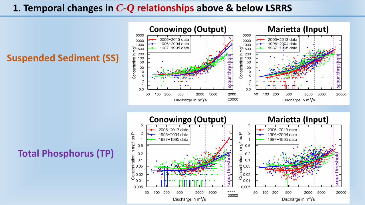
ldTotal Phosphorus (TP)
sco
ur
thre
sho
ld
sco
ur
thre
sho
ld
Conowingo (Output) Marietta (Input)
Suspended Sediment (SS)
Conowingo (Output) Marietta (Input)
1. Temporal changes in C-Q relationships above & below LSRRS
Suspended Sediment (SS) loadings
2. Flow-normalized trends in particulate loadings above & below LSRRS
“Flow-Normalized” Estimates by Season of YearMarietta + Conestoga
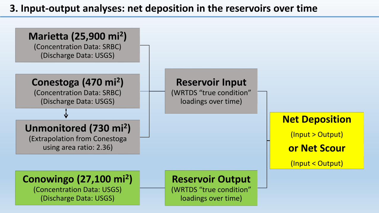
Unmonitored (730 mi2)(Extrapolation from Conestoga
using area ratio: 2.36)
Reservoir Output (WRTDS “true condition”
loadings over time)
Conowingo (27,100 mi2)(Concentration Data: USGS)
(Discharge Data: USGS)
3. Input-output analyses: net deposition in the reservoirs over time
76% of initialslope
32% of initialslope
3. (cont’d) Input-output analyses: sediment storage from mass balance
SS TP TN
• Output/input ratio < 1 net deposition.
• Travel time: we used 35-day moving averages of both input and output to mitigate effects of travel time across the reservoir system.(Results insensitive to selection of averaging time.)
• SS and TP ratios have increased in recent years.
Averages (blue dots) & the 95% confidence intervals (black error bars) (based on estimation with 100 realizations of representative data sets)
• Trends in annual median O/I are qualitatively maintained based on the 100 realizations.
• TP ratios > SS ratios, suggesting that decreasing retention in recent years is more pronounced for the finer (and more P-enriched) sediments.
• TN ratios: recent rise reflects an increasingly larger quantity and fraction of PN in the reservoir output that deserves further study and management consideration.
3. (cont’d) Input-output analyses: uncertainty analysis on O/I ratio
Annual No. of excursions for O/I ratio for different cut-off thresholds
• TN: the recent rise in excursions reflects an increasingly larger quantity and fraction of PN in the reservoir output.
3. (cont’d) Input-output analyses: uncertainty analysis on O/I ratio
Conowingo Dam on 9/12/2011, 3 days after peakdischarge following Tropical Storm Lee (9/1 to 9/5)REF: pubs.usgs.gov/sir/2012/5185/
Total Phosphorus
(TP)
3. Input-output analyses: O/I ratios by flow class
Conowingo Flow ClassesQ1: 25~396 m3/s;
Q2: 399~787 m3/s; Q3: 790~1,464 m3/s;
Q4: 1,467~7,646 m3/s; Q5: 7,674~20,077 m3/s.
Qscour: ~ 11,000 m3/s
• Q4 has dominated the absolute mass delivery of Vw, TN and TP through the system despite its sub-scour status.
• Q4 has also had a major contributionto SS delivery.
Conowingo Flow ClassesQ1: 25~396 m3/s;
Q2: 399~787 m3/s; Q3: 790~1,464 m3/s;
Q4: 1,467~7,646 m3/s; Q5: 7,674~20,077 m3/s.
Qscour: ~ 11,000 m3/s
3. (cont’d) Input-output analyses: % contributions of loads by flow classes
Q: Are these results biased by differential highflow samplings at Marietta and Conowingo?
• The major distinction on highflow sampling lies in 15000-20000 m3/s, for which 3 dates were sampled at Conowingo (i.e., 1996/01/21, 2004/09/20, and 2011/09/08) but not Marietta.
3. (cont’d) Input-output analyses: sensitivity to differential highflow samplings
scour threshold
2011-09-09
2011-09-082004-09-201996-01-21
3. (cont’d) Input-output analyses: sensitivity to differential highflow samplings
Sensitivity analysis
• We have re-run WRTDS model on Marietta and Conowingo by using only those samples with Q < 15000 m3/s.
• Results are consistent with those based on all samples – SS and TP output/input ratio has been rising since the early 2000s.
SS TP
• Inter-annual comparisons of loading and net deposition based on standard WRTDS models are influenced by the particular time history of discharges that happened in a given year as well as the concentration regression surface, i.e., C(Q, tseason).
• To isolate and reveal changes in the concentration regression surface (which we presume to reflect changes in reservoir system function), we select three “stationary” WRTDS models:
• Step 1: Build the standard WRTDS model.
• Step 2: Select three 1-yr-wide C(Q, t) surfaces from the standard model -- 1990, 2000, 2010.
ln(C)Conowingo SS
4. Stationary-model analyses: effects of changing C(Q, tseason) surface
• Step 3: Separately repeat each of these 1-year surfaces over the full record to produce three “stationary” surfaces for the full period of record.
• Step 4: Apply each surface to the same full period of record (of daily Q) to estimate daily C and loads.
• Step 5: Conduct mass-balance analyses on input and output loads.
• Step 6: Establish confidence intervals by re-sampling (with replacement).
Because all scenarios use the same flow record, observed differences in load estimates are due to the difference in the assumed stationary C(Q, tseason).The resulting 3 alternative load estimates (based on models separated by a decade) will reflect impacts that are presumed to be due to a changing system.
4. (cont’d) Stationary-model analyses: effects of changing C(Q, tseason) surface
sco
ur
thre
sho
ldTP Input
sco
ur
thre
sho
ldTP Output
Differences in TP loading vs flow (Q) among three scenarios of stationary regression surface representing 1990, 2000, and 2010reservoir conditions
4. (cont’d) Stationary-model analyses: load vs. Q under 3 reservoir conditions
sco
ur
thre
sho
ld
TP Net Deposition
Differences in net deposition rate vs flow among three scenarios of stationary regression surface representing 1990, 2000, and 2010 reservoir conditions
• Overall, diminished net trapping of TP and SS (similar patterns) has occurred under a range of flow conditions, including flows well below the scour threshold.
• These changes reflect diminished reservoir performance rather than climatic factors such as increased streamflow variability.
4. (cont’d) Stationary-model analyses: load vs. Q under 3 reservoir conditions
Cumulative SS net deposition for a Wet(2011), an Average(2005), and a Dry Year (2001) as predicted using 3 Model Scenarios representing reservoir condition in 1990, 2000 and 2010
Wet Year (2011)No scour if TS Lee had
occurred under the 1990 reservoir
condition
Normal Year (2005)No scour if the high flow had occurred under the 1990 and 2000 reservoir
conditions
Dry Year (2001)(Mildly) reduced net deposition
even for the dry year scenario
4. (cont’d) Stationary-model analyses: storage under 3 reservoir conditions
Major Findings
• This retrospective study has evaluated reservoir performance in the last three decades using different types of modeling approaches, all of which consistently show decreased net deposition of SS and TP in Conowingo Reservoir.
• Decreased reservoir trapping has occurred under a wide range of flow conditions, including sub-scour levels. The 75th~99.5th percentile of flow at Conowingo (high but sub-scour levels) has dominated the absolute mass of delivery through the reservoir.
5. Summary
• Moreover, recent rise in TN output/input ratio may reflect an increasingly larger quantity and fraction of PN in the reservoir output that deserves attention and further study.
• The results are robust based on uncertainty analysis and are insensitive to the differential highflow samplings at Marietta and Conowingo.
Management Implications
• Future progress in Bay restoration will depend on accurate predictions of how SS/TP/TN inputs to the reservoirs will be modulated by processes taking place in the reservoirs.
• Our analyses can help constrain and inform the development of improved predictive models of reservoir performance, and particularly the (possible) incorporation of such models in the ongoing upgrade of the Chesapeake Bay Partnership’s Watershed Model.
• This retrospective study does NOT speak for the issue of future reservoir conditions.
• Additional monitoring and modeling of the reservoir is critically needed, including at least (a) reservoir input and output conditions, (b) bathymetry measurements, (c) nutrient distributions in reservoir bottom sediments, and (d) nutrient transport and fate under different flow conditions.
Output A: “true-condition” daily concentration and load
Use given day’s Q and proximate C observations (Time-Discharge-Season) to estimate the
best “true” estimates of conc. and loadings
For understanding real impacts on the ecosystem
(fluvial and estuarine response; historical effects on living resources)
Output B: “flow-normalized” daily concentration and load
Use full history of given calendar day’s Q with proximate C observations to calculate
“flow-normalized” estimates of conc. and loadings
For assessing progress in management and watershed function
(nutrient and sediment source control, BMPs, land use & cover)
Statistical Method (WRTDS) Hirsch et al., JAWRA (2010); Zhang et al., SOTE (2013)
Reproduced from Zhang et al. (2013)
The WRTDS Model
Conowingo Flow ClassesQ1: 25~396 m3/s;
Q2: 399~787 m3/s; Q3: 790~1,464 m3/s;
Q4: 1,467~7,646 m3/s; Q5: 7,674~20,077 m3/s.
Qscour: ~ 11,000 m3/s
Conowingo Dam on 9/12/2011, 3 days after peakdischarge following Tropical Storm Lee (9/1 to 9/5)REF: pubs.usgs.gov/sir/2012/5185/
SuspendedSediments
(SS)
3. (cont’d) Input-output analyses: O/I ratios by flow class
Conowingo Dam on 9/12/2011, 3 days after peakdischarge following Tropical Storm Lee (9/1 to 9/5)REF: pubs.usgs.gov/sir/2012/5185/
Total Nitrogen(TN)
3. (cont’d) Input-output analyses: O/I ratios by flow class
Conowingo Flow ClassesQ1: 25~396 m3/s;
Q2: 399~787 m3/s; Q3: 790~1,464 m3/s;
Q4: 1,467~7,646 m3/s; Q5: 7,674~20,077 m3/s.
Qscour: ~ 11,000 m3/s
SS Output
Frequency Plots of Ranked Loadings
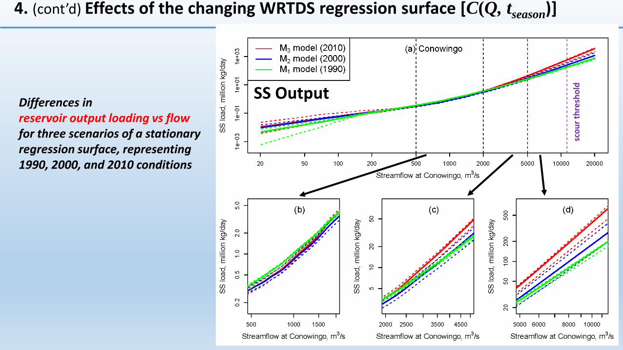
4. (cont’d) Effects of the changing WRTDS regression surface [C(Q, tseason)]
SS Output SS Input SS Net Dep.
TP Output TP Input TP Net Dep.
4. (cont’d) Effects of the changing WRTDS regression surface [C(Q, tseason)]
TN Output TN Input TN Net Dep.
Frequency Plots of Ranked Loadings
Stationary-Model Summary (1)
• Reservoir inputs of SS, TP, and TN have generally declined.
• Reservoir outputs of SS and TP have generally increased.
• Reservoir net deposition of SS and TP has declined greatly.
4. (cont’d) Effects of the changing WRTDS regression surface [C(Q, tseason)]
sco
ur
thre
sho
ldSS OutputDifferences in reservoir output loading vs flowfor three scenarios of a stationary regression surface, representing 1990, 2000, and 2010 conditions
4. (cont’d) Effects of the changing WRTDS regression surface [C(Q, tseason)]
sco
ur
thre
sho
ldSS OutputDifferences in reservoir output loading vs flowfor three scenarios of a stationary regression surface, representing 1990, 2000, and 2010 conditions
4. (cont’d) Effects of the changing WRTDS regression surface [C(Q, tseason)]
sco
ur
thre
sho
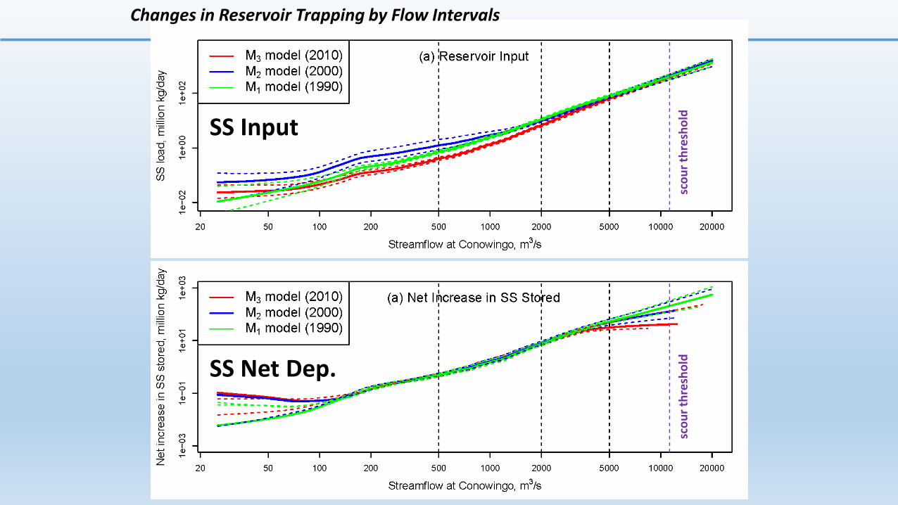
ldSS Net Dep.
sco
ur
thre
sho
ld
SS Input
Changes in Reservoir Trapping by Flow Intervals
sco
ur
thre
sho
ld
SS Net Dep.
4. (cont’d) Effects of the changing WRTDS regression surface [C(Q, tseason)]
Differences in net deposition rate vs flow among three scenarios of a stationary regression surfacerepresenting 1990, 2000, and 2010 conditions