17 January 2013

Page 1 of 22

II. Effects of Riparian Management Strategies on Stream Temperature

Science Review Team Temperature Subgroup

Peter Leinenbach1, George McFadden2, and Christian Torgersen3 (authors listed alphabetically)

1 U.S. Environmental Protection Agency, Seattle, WA

2 U.S. Geological Survey, Seattle, WA 3 Bureau of Land Management, Portland, OR

Background The Science Roundtable Team (SRT) of technical experts was requested by the Interagency Coordinating Subgroup (ICS) to evaluate models that predict changes in shade and stream temperature as a result of the removal of trees in riparian areas. The management concern is that stream temperature in the summer may increase as a result of riparian management activities and negatively affect coldwater fishes, including salmon, trout, and associated aquatic ecosystems. The area of interest includes conifer forests of the Oregon Coast Range, but the findings of the SRT are intended to be applicable to a broader range of forests in western Oregon and Washington. The ICS requested information on what is known and not known about the effects on shade and water temperature of various riparian management strategies that employ no-cut buffers of various widths and thinning of trees at different intensities. In contrast to the well-documented impacts of clearcuts on shade and stream temperature, the effects of partial cutting and removal of trees in riparian areas have not been well studied and are more difficult to predict than the effects of clearcuts. Mechanistic models that predict changes in stream temperature as a result of increases or decreases in solar radiation provide a foundation for addressing the questions posed by the ICS, and empirical studies provide additional insights into the complexities of applying these models in the field. In this document, we summarize pertinent scientific theory and empirical studies to address the following tasks specified by the ICS:

Define the effects of various riparian management strategies on stream function, with a focus on temperature.

• Describe effects associated with “no cut” buffers of various widths and alternative thinning regimes (e.g., skips and gaps, different thinning intensities).

• Characterize the distance at which thinning affects downstream temperature. • Describe how unstable landforms and existing riparian roads can affect the

conclusions reached in the above analysis. To address the management concerns outlined by the ICS, we focus on stream temperature during the summer when reductions in shade due to the removal of trees could potentially cause increases in the maximum or average daily temperature that exceed the thermal tolerances of aquatic organisms (Beschta et al. 1987). We begin by defining the physical factors that influence the thermal regime of streams, and then we specifically examine the scientific literature that describes the effects associated with alternative riparian management strategies. We then explain the complexities of determining downstream impacts of riparian management strategies

17 January 2013

Page 2 of 22

in the stream network. We also identify special considerations for evaluating these effects in the context of landslides and roads in riparian areas. Finally, we identify areas of uncertainty that make it difficult to predict the effects of various riparian management strategies without extensive knowledge of factors that are difficult to quantify and expensive to measure in the field. Factors influencing stream temperature Stream temperature is influenced by multiple anthropogenic and non-anthropogenic factors that occur above the water surface, in the streambed, within the water column, and in the surrounding landscape (Poole and Berman 2001, Caissie 2006) (Figure 1). These factors can be grouped in four general categories: (1) atmospheric conditions, (2) the streambed, (3) stream discharge, and (4) topography (Caissie 2006). The interactions among these factors make predicting changes in stream temperature response to human alteration of the landscape a challenging task, particularly if precise estimates of thermal impacts are required to inform management decisions (Johnson 2003; Hester and Doyle 2011). Heat exchange processes in streams The interactions among factors that influence water temperature in streams are complex, but the actual physics of stream heating can be summarized relatively simply as exchanges of energy at the air/water surface and at the streambed/water interface (Figure 2). The relative importance of the various heat exchange processes in Figure 2 varies with respect to the factors identified in Figure 1. However, solar radiation is generally the dominant component of the energy budget in terms of heat gain (Moore and Wondzell 2005, Cassie 2006). Inputs of heat energy from solar radiation can be large compared to the losses associated with heat exchange. Therefore, most of the solar energy is stored in the stream, thereby causing an increase in water temperature in a downstream direction. Accordingly, the most efficient method to maintain low stream temperatures is to reduce heat loading from solar radiation. Shade prevents stream warming by reducing inputs of heat energy from solar radiation. The removal of heat energy from the stream requires heat exchange of the water with the surrounding environment through which energy moves out of the “warm” stream via processes associated with the second law of thermodynamics (i.e., energy travels from high to low concentrations). Inputs of cold water from the streambed, seepage areas on the stream bank, and tributaries can be large components of the net energy budget and can help cool the stream on hot summer days if they are sufficiently large relative to the stream discharge (Wondzell 2012). Energy gained from solar radiation also leaves the stream through long-wave radiation, evaporation, convection (air and water), and conduction (air, water, streambed) (Figure 1) (Caissie 2006). Stream temperature and riparian management strategies The effects of riparian vegetation on shade and stream temperature have been studied extensively, and it is generally accepted that removing trees in riparian areas reduces the amount of shade which leads to increases in thermal loading to the stream (Moore and Wondzell 2005).

17 January 2013

Page 3 of 22

This increase in thermal loading from direct solar radiation after the removal of shade may or may not lead to measurable increases in stream temperature depending on the net effect of the multiple factors described in the following sections. What are factors are most relevant? We focus on shade and the factors that influence its spatial extent, temporal duration, and quality. The primary factors that influence shade are riparian vegetation (Groom et al, 2011b) and the surrounding terrain (Allen et al. 2007). Note that riparian vegetation, upland shading, and aspect (i.e., stream orientation) are grouped under the general category of topography because both trees and the surrounding landscape constitute vertical structure that affects the transmission of solar radiation to the stream (Figure 1). We also consider (1) the physical characteristics of the stream itself and how they affect heat flux at the water surface, and (2) the role of direct transfer of energy to and from the stream through groundwater, tributary inflow, and hyporheic exchange. Why are these factors important? Although many other factors affect stream temperature (Figure 1), we focused on (1) shade, (2) heat flux at the water surface, and (3) groundwater–surface water interactions because these factors are often directly associated with riparian management activities (Webb et al. 2008). Other factors are not addressed because (1) they are difficult to measure in the field and incorporate into predictive models, and (2) they compose a relatively small part of the heat budget in the streams that are most likely to be encountered in the forested landscapes pertinent to this report (Johnson 2003). Shade in riparian areas In order to assess the ability of riparian vegetation to create effective shade over a stream, three characteristics of the “shade” need to be evaluated: (1) spatial extent, (2) temporal duration, and (3) quality. Shade spatial extent is the spatial area over which a shadow is cast over a stream. Shade temporal duration is the length of time during which a portion of stream is shaded. Shade quality is a function of the canopy density (including the stems), where lower canopy density is associated with lower shade quality. The removal or modification of trees in riparian areas can affect the spatial extent, temporal duration, and quality of shade on a stream. Vegetation height and topography The height of the vegetation directly influences the spatial extent of shade. On flat ground, the distance over which a tree can cast a shadow during the summer in the Pacific Northwest varies from approximately 50-200% of the tree height, depending on the time of day (see discussion below on temporal variability). Depending on sun angle and tree height, there is a threshold distance from the stream at which shadows from even the tallest trees will no longer reach the stream from mid-day to late afternoon when thermal loading from solar radiation is greatest. Wherever streambanks are higher than the stream, the effective height of vegetation includes not just the height of the tree but also the elevation of its base above the stream. Thus, shadow

17 January 2013

Page 4 of 22

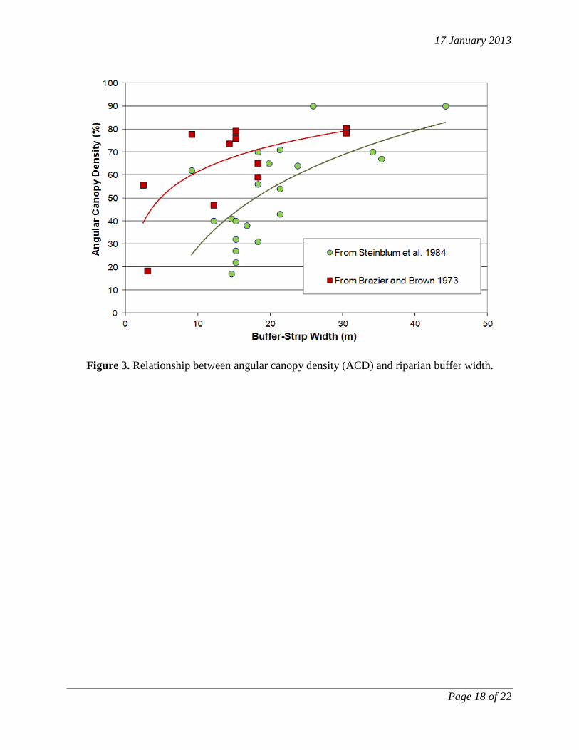
length is longer for vegetation located on streambanks above the stream. In steep, narrow headwater catchments, a large proportion of shade may be created by topographic relief alone; however, at broader scales, and at most locations within a watershed, the largest component of shade is typically derived from riparian vegetation (Allen et al. 2007, Allen 2008). Because shade conditions in streams are a function of shade produced by the vegetation and shade produced from topography, both factors must be considered in evaluating potential effects of removing trees in riparian areas. Density of vegetation The density of vegetation in riparian areas affects shade and thermal loading to a stream due to the penetration of solar radiation through gaps in the canopy and among the branches and stems (Brazier and Brown 1973, DeWalle 2010). Riparian stands with few trees and low canopy and branch density reduce shade quality. The removal of vegetation through “thinning” activities results in an initial lowering of the vegetation density in the riparian stand. In low-density stands (i.e., more open stands), wider buffers can compensate for decreased canopy density and help achieve the same shade quality as would be achieved given similar vegetation with a closer spacing of trees. Width of buffer The width of the band of vegetation along the stream bank influences the amount of solar radiation that reaches the stream. Wide buffers create more shade than narrow buffers, as measured by angular canopy density (Brazier and Brown 1973, Wooldridge and Stern 1979, Steinblums et al. 1984, Beschta, et al. 1987). However, there is a high degree of variability in this relationship, particularly at narrower buffer widths where the effect on shade is greatest. For instance, data from Brazier and Brown (1973) and Steinblums et al. (1984) indicate that a 15-m buffer width might provide anywhere from 18 to 80% shading (Figure 3). In addition, these studies also showed that 75-90% shade can be achieved with a wide range of buffer widths, ranging from approximately 9 to 43 m. The high variability in buffer width and shade condition is a function of the many variables that influence the amount of shade produced by riparian vegetation. As described above, low-density stands with limited vertical distribution of branches and foliage may require wider buffer widths to produce the same amount of shade as high-density stands. Temporal variability Shade duration is dependent on day of the year and the height and distance at which the shade-producing feature is located from the stream. Shade duration can be calculated based on physical attributes of the tree (i.e., height and distance to stream) and the location of the sun in the sky, which varies daily and seasonally, and the azimuth of the stream. The intensity of solar radiation on the surface of the earth also varies daily and seasonally based on the vertical angle of the sun in the sky. The shadow length from riparian vegetation is the shortest at mid-day when the sun is high in the sky, and the shadow length increases during other parts of the day as the sun is lower in the sky. In the Pacific Northwest, the greatest amount of energy generally occurs between the hours of 10:00 to 14:00 and in July and August (Beschta et al 1987). However, heat loading

17 January 2013

Page 5 of 22

from solar radiation during other periods of the day constitutes a significant part of the energy budget (~40%) and therefore is influential on stream temperature. Tools that are typically used to measure and model solar radiation incorporate both the surrounding topography (e.g., aspect and elevation) as well as daily and seasonal variation (Moore et al. 2005, Allen et al. 2007, Boyd and Kasper 2003). These methods provide estimates of total shortwave energy for a given day or time period. Such estimates of total shortwave energy are necessary in order to compare the thermal impacts of riparian management scenarios. Stream channel dimensions and heat flux at the water surface The effect of solar radiation at the stream surface on water temperature depends on stream width, and depth, and the flow velocity (Beschta et al. 1987, Sullivan et al. 1990). For a given stream discharge, a shallower, wider stream will heat up faster than a deeper, narrower stream, so it is important to consider the morphology of the channel itself in determining the potential effects of increased solar radiation resulting from riparian management strategies. Furthermore, the exchange of heat energy to the stream from solar radiation depends on the length of stream that is exposed and the time that it takes for water to pass through that area (i.e., a function of velocity). The shadow length associated with a short tree might be sufficient to “cast a shadow” over a narrow stream channel, but this same tree may be insufficient to shade a wider stream channel. Accordingly, stream width is an important factor to consider in determining thermal loading associated with a particular riparian stand. Groundwater and surface water interactions Groundwater inputs, tributary inflow, and hyporheic exchange can directly influence stream temperature because they involve advective transfer of relatively cool or warm water to the stream. The size of the effect is a function of the amount of water entering (or exchanged with) the stream relative to the stream discharge (Johnson and Jones 2000, Story et al. 2003, Wondzell 2006, Wondzell 2012) and the difference in temperature between the stream and the inflowing water. For example, small amounts of cold water can have large effects on stream temperature in warm streams if they are large relative to the size of the receiving stream’s discharge or if they are very cold relative to the receiving stream’s temperature. Such cold-water inputs can be distinct point sources (e.g., groundwater seeps), or they can be diffuse (e.g., hyporheic exchange) (Poole and Berman 2001; Poole et al. 2001, Wondzell 2012). If the net effect of these inputs over a given stream distance is large relative to the stream discharge, they can have significant effects on downstream reaches. Thus, the magnitude of temperature response associated with riparian management is directly related to these processes, which can either increase or decrease stream temperature. Effects associated with riparian management strategies Removal of trees in riparian areas increases shortwave thermal loading to streams through its effects on (1) shade quality (i.e., thinning of the stand to reduce the stand density), and (2) shade temporal duration (i.e., reducing the average vegetation height as a result of thinning from “above”) (Groom et al 2001b). The specific shade response to tree removal depends on pre-harvest vegetation, including its composition, structure, and location relative to the stream, and

17 January 2013

Page 6 of 22

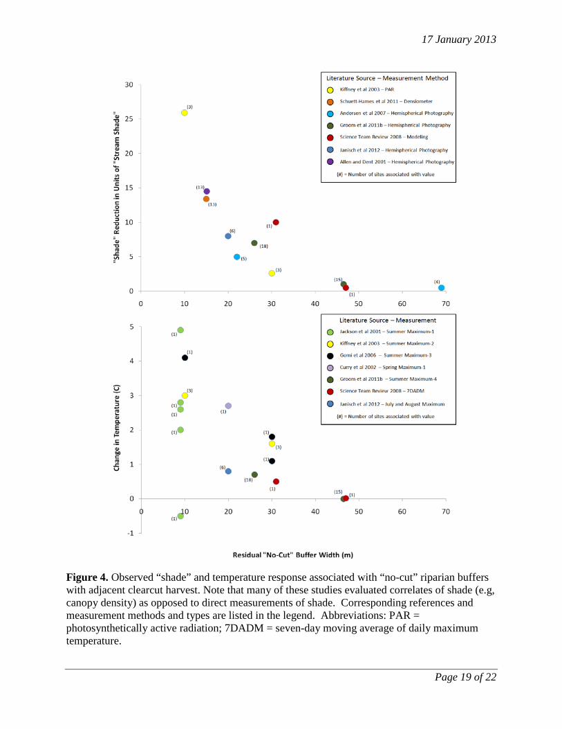
on the number and location of trees that are removed. Therefore, specific trends described below only provide approximate guidelines of shade conditions associated with various buffer conditions given the variability of conditions in the forests pertinent to this report. In addition, the effects of riparian management on stream temperature are even more variable (Moore et al. 2005a, Moore et al. 2005b, Moore and Wondzell 2005, Janisch et al. 2012). No-cut buffers adjacent to clearcut harvest units Substantial effects on shade have been observed with “no-cut” buffers ranging from 20 to 30 m (Brosofske et al. 1997, Kiffney et al. 2003, Groom et al. 2011b), and small effects were observed in studies that examined “no-cut” buffers 46 m wide (Science Team Review 2008, Groom et al. 2011a). For “no-cut” buffer widths of 46-69 m, the effects of tree removal on shade and temperature were either not detected or were minimal (Anderson et al. 2007, Science Team Review 2008, Groom et al. 2011a, Groom et al. 2011b) (Figure 4). The limited response observed in these studies can be attributed to the lack of trees that were capable of casting a shadow >46 m during most of the day in the summer (Leinenbach 2011; Appendix C of this document). Reductions in shade and increases in stream temperature were more apparent at ~30 m “no-cut” buffer widths, as compared to the 46-69 m wide buffers, but the magnitude and direction of response was highly variable for both shade and stream temperature (Kiffney et al. 2003, Gomi et al. 2006, Science Team Review 2008, Groom et al. 2011a, Groom et al. 2011b). At “no-cut” buffer widths of <20 m, there were pronounced reductions in shade and increases in temperature, as compared to wider buffer widths. The most dramatic effects were observed at the narrowest buffer widths (≤10 m) (Jackson et al. 2001, Curry et al. 2002, Kiffney et al. 2003, Gomi et al. 2006, Anderson et al. 2007). Thinning in riparian buffers adjacent to clearcut harvest units Reductions in shade and increases in stream temperature were associated with thinning activities occurring within riparian buffers, along with the narrowing of the buffer (Mellina et al. 2002, Macdonald et al. 2003, Wilkerson et al. 2006, Science Team Review 2008, Kreutzweiser et al. 2009) (Figure 5). However, the response varied from no effects to large effects which appeared to be related to differences in the intensity of thinning, with stronger effects associated with higher thinning intensities. However, the limited number of studies that have specifically evaluated thinning in riparian buffers makes it difficult to generalize, particularly given the many different possible combinations of thinning intensity and buffer width. No-cut buffers adjacent to thinning harvest units The width of the inner “no-cut” riparian buffer was shown to affect the potential consequences of thinning in the “outer” buffer regions, with wider “no-cut” buffers resulting in lower reductions in stream shade conditions (Anderson et al. 2007, Science Team Review 2008, Park et al 2008) (Table 1). In addition, the canopy density of the inner “no-cut” buffer zone appeared to have an ameliorating effect on thinning activities within the “outer” thinning buffer zone, with higher “protection” associated with greater canopy densities in the inner zone. Finally, higher residual vegetation densities within the “outer” thinning zone were shown to result in less shade loss. Once again, the limited number of studies that have specifically evaluated these buffer conditions

17 January 2013

Page 7 of 22

make it difficult to generalize, particularly given the many different possible combinations of thinning intensity, buffer widths, and stream sizes. Other associated effects Secondary effects of thinning in riparian areas can potentially reduce shade and potentially lead to increases in stream temperature. For example, trees that are left after thinning may be vulnerable to blowdown (Chan et al. 2006), which has been shown to decrease shade and increase stream temperatures (MacDonald et al. 2003). Similarly, “no-touch” riparian buffers have also been shown to be vulnerable to windthrow following harvest activities (Jackson et al. 2007), resulting in much lower stream shade conditions (Schuett-Hames et al. 2011). Windthrow effects can be long term. For example, windthrow was shown to impede the “recovery” of stand density (i.e., shade conditions) for over eight years following both “heavy” and “moderate” thinning treatments (Curtis Relative Density [RD] of 8.3 and 16.0, respectively), but recovery was observed over the same period in “lightly” thinned stands (RD of 27.8). Secondary effects of thinning and associated road building on microclimate, sediment loads to the stream, and subsurface drainage patterns adjacent to riparian areas are poorly understood but may influence advective transfer and heat exchange in water that enters the stream as shallow groundwater (Story et al. 2003, Brosofske et al. 1997, Anderson et al. 2007). Potential downstream effects The spatial extent to which riparian management affects stream temperature downstream of harvest units depends on the spatial context of the stream reach in terms of hydrology and geomorphology and how these factors interact in the stream heat budget (Poole et al. 2001, Johnson 2003). For example, in stream reaches with cold tributary inflows and groundwater inputs that constitute a large percentage of the stream discharge (i.e., “gaining” reaches), the distance may be short to bring the temperature back down to what it would have been prior to the reduction in shade resulting from the removal of trees (Story et al. 2003). Similarly, reaches with extensive hyporheic exchange (Wondzell 2006, Wondzell 2012) via the streambed and floodplain may show no effects of increased solar radiation on stream temperature (Janisch et al. 2012). In contrast, bedrock-dominated stream channels are likely to require very long recovery distances because they are not buffered by hyporheic exchange (Johnson and Jones 2000). Thus, it is not possible to characterize the exact distance at which thinning activities will affect downstream temperature without accounting for all of the factors that influence stream temperature. However, the rate of heat loss via convection and evaporation at the surface of small streams is very slow, as compared to the heat exchange rate associated with solar radiation loading. Therefore, the heat added to a stream by the sun will not be readily dissipated, and the distance over which elevated temperatures may extend downstream may be much longer than the length of the “treatment”. Considerations for unstable landforms and existing roads In riparian areas with unstable landforms and existing roads, precautions are necessary to ensure that enough shade will be available in the event of future landslides that could remove forest vegetation and reduce shade on the stream. Thus, the removal of shade needs to be evaluated on

17 January 2013

Page 8 of 22

the basis of how much shade is currently present because further riparian management activities in a “disturbed” stand can have a larger impact on shade conditions than what would be expected from the same level of disturbance in an “undisturbed” stand (Chan et al. 2004b). Disturbed stands that have been subjected to tree removal before thinning activities may already have low canopy density, and hence already provide limited shade. Furthermore, the removal of trees on unstable slopes may lead to increased vulnerability of neighboring trees to windthrow and landslides, which both can lead to reductions in shade and potential increases in stream temperature (Pollock et al. 2009). All kinds of landslides can topple and remove trees and, therefore, have the potential to reduce canopy density and shade (Oregon Department of Geology and Mineral Resources 2008). Debris flows are also of concern because they often remove stream- adjacent trees, alluvium, wood and soil along the debris flow track, creating a wide, shallow and generally featureless bedrock channel. Riparian shade is removed, the growth of future stream-adjacent trees is inhibited because soil is lacking, the cooling effect of hyporheic exchange is minimized because there is no alluvium, and the potential for future accumulations of alluvium is reduced because there is little large wood in the system to retain alluvium, and there are no large riparian trees to provide large wood (Montgomery 1997, Pollock et al. 2009). Depositional areas from debris flows also have the potential to inundate riparian floodplain forests with water and sediment and cause increased tree mortality. Thus, where debris flows and landslides have occurred, the effects on stream temperature may last for centuries. Although estimates of impacts of thinning near existing roads and unstable landforms need to be conservative to account for potential future losses of shade, it may be very difficult to weigh the advantages and disadvantages of such thinning activities within the broader context of landscape disturbance and its role in aquatic ecosystems (Reeves et al. 1995, Montgomery 1997). For example, landslides and debris flows can reduce shade, but may provide large accumulations of wood and sediment, which can have variable effects on stream geomorphology, depending on the location and condition of the pre-existing habitat where deposition occurs (May and Gresswell 2003). Thus, in the context of landscape management, there are multiple physical effects of landslides and debris flows that need to be considered, and these effects vary with landscape position. What is not known or uncertain Extensive research on the effects of forest management on shade and stream temperature provides a foundation for predicting the effects of thinning in riparian areas. However, because the effects of thinning are lesser in magnitude compared to complete removal of riparian vegetation, landscape context (e.g., geology, geomorphology, and hydrology) plays a greater role and can make it more difficult to determine cause and effect (Thompson 2005). Furthermore, thinning may occur at different intensities and in various spatial configurations which may be difficult to model and evaluate experimentally. There are no examples of studies in the literature on the effects of riparian thinning on stream temperature that match the specific characteristics of management activities likely to occur in riparian areas on federal forest lands. Field studies that can address these challenges may require watershed-scale, long-term manipulative experiments to detect effects over spatial and temporal scales that are relevant to the ecological, hydrological, and geomorphological processes of

17 January 2013

Page 9 of 22

interest. However, shorter-term studies that evaluate potential effects of thinning intensity and buffer width on shade and stream temperature can be conducted by substituting space for time (Pickett 1989) in which sites representing a wide range of thinning intensities and buffer widths are examined in relation to the relative amounts of shade that they produce. Although the results of such studies cannot elucidate causal relationships, they would still provide a foundation for evaluating potential downstream cooling distances in riparian areas under various thinning scenarios. These field studies could be designed to test hypotheses about where downstream cooling distances would be expected to be long or short. Recently available technologies such as lidar remote sensing, thermal IR remote sensing, and distributed temperature sensing could be used to better quantify shade and evaluate stream temperature response to various thinning treatments (Lutz et al. 2012, Torgersen et al. 2012). Spatially explicit models and landscape analysis tools that consider many different factors at multiple spatial and temporal scales may be used to evaluate potential cumulative effects of riparian management scenarios (Cissel et al. 1999, Benda et al. 2007). However, these landscape analysis tools need to be better integrated with stream temperature models (see Allen et al. 2007). Many different models exist for predicting stream temperature response to changes in shade; for descriptions of these models and their relative strengths and weaknesses, see Caissie 2006, Allen et al. 2007, Chapter 2 in Allen 2008, Webb et al. 2008, and Torgersen et al. 2012. The most commonly applied stream temperature model in western Oregon is HeatSource (Boyd and Kasper 2003), which was developed by the Oregon Department of Environmental Quality and the U.S. Environmental Protection Agency. This model has been used effectively to evaluate effects of shade on water temperature in streams of various sizes and types, and it is currently the most accessible stream temperature modeling tool for land managers because of the availability of technical support from government agencies. A limitation of HeatSource and most other stream temperature models is that they require data on the physical and hydrological characteristics of the stream (width, depth, and velocity) which may be difficult to acquire in the field, particularly in forested streams that may be inaccessible due to dense vegetation, steep topography, and a lack of roads. Another modeling tool that is increasingly used by federal forest managers is NetMap (Benda et al. 2007; www.netmaptools.org). It is important to note, however, that NetMap does not predict stream temperature; it provides information only on spatial variability of thermal loading as a function of shade from trees (based on tree height and buffer width) and/or the surrounding topography. NetMap has immense potential for evaluating the potential effects of riparian thinning on thermal loading across landscapes; however, these predictions may be limited by the data on forest structure (i.e., stem and canopy density) and topography (e.g., digital elevation models) on which the model is based (see Appendix D on the appropriate use of geospatial data and models in resource management). It is possible that tools such as NetMap will provide more precise estimates of thermal loading based on lidar-derived high-resolution measurements of forest structure and topography; however, these datasets are not widely available. Field studies are needed to “ground-truth” NetMap predictions of thermal loading in varied landscape settings and with different spatial scales of forest structure and topographic data (e.g., 1-5-m lidar data versus 10- and 30-m digital elevation models).

17 January 2013

Page 10 of 22

Field studies as well as the spatially explicit modeling and landscape analysis tools described above are needed to address the following uncertainties associated with predicting the effects of thinning in riparian areas on shade and stream temperature: Effects of thinning intensity and “skips and gaps” The intensity of thinning activities has an impact on the amount of shade produced by the riparian stand. Thinning from “below” (i.e., removing small trees) primarily affects shade quality by increasing the transmission of solar radiation from the side, whereas thinning from “above” by removing large trees that cast long shadows most likely affects both shade quality and duration. Implementing a “skips and gaps” thinning scheme (i.e., leaving patches of undisturbed riparian forest along the stream) may reduce shade conditions and potentially increase stream temperature; however, this scenario may have less of an impact if the cut patches are located farther away from the stream. Additional field studies and spatially explicit modeling in a variety of forest and hydrological settings are needed in this area. Groundwater and hyporheic exchange Tools and techniques for measuring the vertical and horizontal structure of forest vegetation and the underlying ground surface are advancing rapidly (e.g., ground-based and airborne lidar), and it is likely that within the next decade, it will be possible to develop highly detailed shade models for entire small watersheds. Such information may solve many of the problems associated with measuring the transmission of solar radiation through the forest to the stream. However, the most significant challenge to predicting the effects of thinning in riparian areas is the lack of information on processes below the water surface and in the floodplain. This problem has been addressed in modeling of stream temperature in larger rivers by using remote sensing of water temperature to identify thermal anomalies associated with groundwater and surface water interactions which then can be incorporated into a spatially explicit stream temperature model (Boyd and Kasper 2003). Unfortunately, airborne remote sensing of water temperature is not possible in small forest streams where dense overhanging vegetation may block the view of the stream. Thus, in these streams, it will be necessary to use in situ methods and hydrologic modeling to quantify thermal heterogeneity in water temperature associated with groundwater inputs and hyporheic exchange. With the recent dramatic improvements in stream temperature sensor technology (e.g., mobile probes and temperature-sensitive fiber-optic cable), it is now possible to quantify thermal heterogeneity in small streams at relatively low cost. These new techniques are capable of mapping stream temperature at a fine spatial resolution (1 m) over several kilometers and can be used to improve the accuracy and precision of (1) models that predict potential effects of riparian thinning on stream temperature and (2) monitoring of water temperature in response to riparian forest management. Acknowledgments Comments from S. Wondzell and M. Fitzpatrick on earlier versions of this document greatly improved the clarity and precision of the material presented in this summary. Any use of trade, product, or firm names is for descriptive purposes only and does not imply endorsement by the U.S. Government.

17 January 2013

Page 11 of 22

17 January 2013

Page 12 of 22

References Allen D., W. Dietrich, P. Baker, F. Ligon, and B. Orr. 2007. Development of a mechanistically

based, basin-scale stream temperature model: Applications to cumulative effects modeling. USDA Forest Services Gen. Tech. Rep. PSW-GTR-194.

Allen, D. M. 2008. Development and application of a process-based, basin-scale stream temperature model. Ph.D. dissertation. University of California, Berkeley.

Allen M., and L. Dent. 2001. Shade conditions over forested streams in the Blue Mountain and Coast Range georegions of Oregon. ODF Technical Report #13.

Anderson P. D., D. J. Larson, and S.S Chan. 2007. Riparian buffer and density management influences on microclimate of young headwater forests of western Oregon. Forest Science 53(2):254-269.

Benda, L., D. J. Miller, K. Andras, P. Bigelow, G. Reeves, and D. Michael. 2007. NetMap: A new tool in support of watershed science and resource management. Forest Science 52:206-219.

Beschta, R. L., R. E. Bilby, G. W. Brown, L. B. Holtby, and T. D. Hofstra. 1987. Stream temperature and aquatic habitat: Fisheries and forestry interactions. Pages 191-232 in E. O. Salo and T. W. Cundy, editors. Streamside management: Forestry and fishery interactions. University of Washington, Institute of Forest Resources, Seattle, USA.

Boyd, M., and B. Kasper. 2003. Analytical methods for dynamic open channel heat and mass transfer: Methodology for Heat Source Model Version 7.0. www.deq.state.or.us/wq/TMDLs/tools.htm. Viewed 1 July 2008.

Brazier, J.R. and G.L. Brown. 1973. Buffer strips for stream temperature control. Oregon State University: Forest Research Lab Research Paper 15.

Brosofske, K.D., J. Chen, R.J. Naiman and J.F. Franklin. 1997. Harvesting effects on microclimatic gradients from small streams to uplands in western Washington. Ecological Applications, 7:1188–1200.

Caissie, D. 2006. The thermal regime of rivers: A review. Freshwater Biology 51:1389–1406. Chan S., P. Anderson, J. Cissel, L. Larson, and C. Thompson. 2004a. Variable density

management in riparian reserves: lessons learned from an operational study in managed forests of western Oregon, USA. Forest, Snow and Landscape Research 78(1/2):151-172.

Chan S., D. Larson, and P. Anderson. 2004b. Microclimate pattern associated with density management and riparian buffers. An interim report on the riparian buffer component of the Density Management Studies.

Chan S.S., D.J. Larson, K. G. Maas-Herner, W.H. Emmingham, S. R. Johnston, and D. A. Mikowski. 2006. Overstory and understory development in thinned and underplanted Oregon Coast Range Douglas-fir stands. Canadian Journal of Forest Research 36:2696-2711.

Cissel, J. H., F. J. Swanson, and P. J. Weisberg. 1999. Landscape management using historical fire regimes: Blue River, Oregon. Ecological Applications 9:1217-1231.

Cristea N., and J. Janisch. 2007. Modeling the effects of riparian buffer width on effective shade and stream temperature. Washington Department of Ecology Publication No. 07-03-028:1–64.

Curry R.A., D. A. Scruton, and K. SD. Clarke. 2002. The thermal regimes of brook trout incubation habitats and evidence of changes during forestry operations. Canadian Journal of Forest Research 32: 1200–1207.

17 January 2013

Page 13 of 22

DeWalle, D.R. 2010. Modeling stream shade: Riparian buffer height and density as important as buffer width. Journal of the American Water Resources Association 46:2 323-333.

Gomi T., D. Moore, and A.S. Dhakal. 2006. Headwater stream temperature response to clear-cut harvesting with different riparian treatments, coastal British Columbia. Water Resources Research 42, W08437.

Groom J. D., L. Dent, L. and Madsen. 2011a. Stream temperature change detection for state and private forests in the Oregon Coast Range. Water Resources Research 47, W01501, doi:10.1029/2009WR009061.

Groom J. D., L. Dent, L. Madsen, J. Fleuret. 2011b. Response of western Oregon (USA) stream temperatures to contemporary forest management. Forest Ecology and Management 262(8):1618–1629.

Hester, E.T and M.W. Doyle. 2011. Human impacts to river temperature and their effects on biological processes: A quantitative synthesis. Journal of the American Water Resources Association 47(3): 571-587.

Jackson, C.R., D.P. Batzer, S.S. Cross, S.M. Haggerty and C.A. Sturm. 2007. Headwater streams and timber harvest: Channel, macroinvertibrate, and amphibian response and recovery. Forest Science 53(2):356–370.

Jackson, C.R., C.A. Sturm, and J.M. Ward. 2001. Timber harvest impacts on small headwater stream channels in the Coast Ranges of Washington. Journal of the American Water Resources Association 37(6):1533–1549.

Janisch, J. E., S. M. Wondzell, and W. J. Ehinger. 2012. Headwater stream temperature: Interpreting response after logging, with and without riparian buffers, Washington, USA. Forest Ecology and Management, doi:10.1016/j.foreco.2011.12.035.

Johnson, S. L. 2004. Factors influencing stream temperatures in small streams: substrate effects and a shading experiment. Canadian Journal of Fisheries and Aquatic Sciences 61:913-923.

Johnson, S. L., and J. A. Jones. 2000. Stream temperature responses to forest harvest and debris flows in western Cascades, Oregon. Canadian Journal of Fisheries and Aquatic Sciences 57:30-39.

Johnson, S.L. 2003. Stream temperature: Scaling of observations and issues for modeling. Hydrological Processes 17: 497–499.

Kiffney, P. M., J. S. Richardson, J. P. Bull. 2003. Responses of periphyton and insect consumers to experimental manipulation of riparian buffer width along headwater streams. Journal of the American Water Resources Association 40:1060-1076.

Kreutzweiser, D. P., S. S. Capell, and S.B. Holmes. 2009. Stream temperature responses to partial-harvest logging in riparian buffers of boreal mixedwood forest watersheds. Canadian Journal of Forest Research 39:497–506.

Leinenbach, P., 2011. Technical analysis associated with SRT Temperature Subgroup to assess the potential shadow length associated with riparian vegetation.

Lutz, J. A., K. A. Martin, and J. D. Lundquist. 2012. Using fiber-optic distributed temperature sensing to measure ground surface temperature in thinned and unthinned forests. Northwest Science 86:108-121.

Macdonald, J.S., E.A. MacIsaac, and H.E. Herunter. 2003. The effect of variable-retention riparian buffer zones on water temperatures in small headwater streams in sub-boreal forest ecosystems of British Columbia. Canadian Journal of Forest Research 33(8): 1371–1382.

17 January 2013

Page 14 of 22

May, C. L., and R. E. Gresswell. 2003. Processes and rates of sediment and wood accumulation in headwater streams of the Oregon Coast Range, USA. Earth Surface Processes and Landforms 28:409-424.

Mellina. E., R.D. Moore, S.G. Hinch, J. S. Macdonald. 2002. Stream temperature responses to clearcut logging in British Columbia: the moderating influences of groundwater and headwater lakes. Canadian Journal of Fisheries and Aquatic Sciences 59:1886–1900.

Montgomery, D. R. 1997. What's best on the banks? Nature 388:328-329. Moore, R.D., Spittlehouse, D.L., Story, A., 2005a. Riparian microclimate and stream

temperature response to forest harvesting: A review. Journal of the American Water Resources Association 41: 813–834.

Moore, R.D., Sutherland, P., Gomi, T., Dhakal, A.S., 2005b. Thermal regime of a headwater stream in a clear-cut, coastal British Columbia, Canada. Hydrological Processes 19: 2591–2608.

Moore, R.D., Wondzell, S.M., 2005. Physical hydrology and the effects of forest harvesting in the Pacific Northwest: A review. Journal of the American Water Resources Association 41: 763–784.

Oregon Department of Geology and Mineral Industries. 2008. Landslide hazards in Oregon. Oregon Geology Fact Sheet. www.OregonGeology.com. Portland, Oregon.

Pickett, S. T. A. 1989. Space-for-time substitution as an alternative to long-term studies. Pages 110-135 in G. E. Likens, editor. Long-term studies in ecology: Approaches and alternatives. Springer-Verlag, New York.

Pollock, M. M., T. J. Beechie, M. Liermann, and R. E. Bigley. 2009. Stream temperature relationships to forest harvest in western Washington. Journal of the American Water Resources Association 45:141-156.

Poole, G. C., and C. H. Berman. 2001. An ecological perspective on in-stream temperature: Natural heat dynamics and mechanisms of human-caused thermal degradation. Environmental Management 27:787-802.

Poole, G. C., J. Risley, and M. Hicks. 2001. Spatial and temporal patterns of stream temperature. Issue Paper 3, EPA Region 10 Temperature Water Quality Criteria Guidance Development Project, U.S. Environmental Protection Agency, Portland, Oregon.

Reeves, G. H., L. E. Benda, K. M. Burnett, P. A. Bisson, and J. R. Sedell. 1995. A disturbance-based ecosystem approach to maintaining and restoring freshwater habitats of evolutionarily significant units of anadromous salmonids in the Pacific Northwest. Pages 334-349 in J. L. Nielsen, editor. Evolution and the aquatic ecosystem: Defining unique units in population conservation. American Fisheries Society, Bethesda.

Schuett-Hames., D., A. Roorbach, and R. Conrad. 2011. Results of the Westside Type N Buffer Characteristics, Integrity, and Function Study. CEMR Final Report. December 14, 2011

Science Team Review. 2008. Western Oregon Plan Revision (WOPR). Draft Environmental Impact Statement. Science Team Review; www.blm.gov/or/plans/wopr/files/Science_Team_Review_DEIS.pdf.

Steinblums, I.J., H.A. Froehlich, and J.K. Lyons. 1984. Designing stable buffer strips for stream protection. Journal of Forestry 82(1):49-52.

Story, A., R.D. Moore, and J.S. Macdonald. 2003. Stream temperatures in two shaded reaches below cutblocks and logging roads: Downstream cooling linked to subsurface hydrology. Canadian Journal of Forest Research 33:1383–1396.

17 January 2013

Page 15 of 22

Sullivan, K., J. Tooley, K. Doughty, J.E. Caldwell, and P. Knudsen. 1990. Evaluation of prediction models and characterization of stream temperature regimes in Washington. Timber/Fish/Wildlife Rep. No. TFW-WQ3-90-006. Washington Dept. of Natural Resources, Olympia, Washington. 224 pp.

Thompson, J. 2005. Keeping it cool: Unraveling the influences on stream temperature. Science Findings. Pacific Northwest Research Station, USDA Forest Service, Portland, OR.

Torgersen, C.E., Ebersole, J.L., Keenan, D.M. 2012. Primer for identifying cold-water refuges to protect and restore thermal diversity in riverine landscapes: U.S. Environmental Protection Agency, EPA 910-C-12-001, p. 91.

Webb, B. W., D. M. Hannah, R. D. Moore, L. E. Brown, and F. Nobilis. 2008. Recent advances in stream and river temperature research. Hydrological Processes 22:902–918.

Wilkerson E., J.M. Hagan, D. Siegel, and A.A. Whitman. 2006. The Effectiveness of different buffer widths for protecting headwater stream temperature in Maine. Forest Science 52(3):221–231.

Wondzell, S.M., 2006. Effect of morphology and discharge on hyporheic exchange flows in two small streams in the Cascade Mountains of Oregon, USA. Hydrological Processes 20: 267–287. doi: 10.1002/hyp.5902

Wondzell, S. M. 2012. Hyporheic zones in mountain streams: Physical processes and ecosystem functions. Stream Notes (January-April), Stream Systems Technology Center, Rocky Mountain Research Station, U.S. Forest Service, Fort Collins, Colorado, USA.

Wooldridge, D.D. and D. Stern. 1979. Relationships of silvicultural activities and thermally sensitive forest streams. University of Washington, College of Forest Resources, Report DOE 79-5a-5. 90 p.

17 January 2013

Page 16 of 22

Figure 1. Factors influencing the thermal regime of rivers and streams (Caissie 2006).

17 January 2013

Page 17 of 22

Figure 2. River and stream heat exchange processes (Caissie 2006).

17 January 2013

Page 18 of 22

Figure 3. Relationship between angular canopy density (ACD) and riparian buffer width.

17 January 2013

Page 19 of 22

Figure 4. Observed “shade” and temperature response associated with “no-cut” riparian buffers with adjacent clearcut harvest. Note that many of these studies evaluated correlates of shade (e.g, canopy density) as opposed to direct measurements of shade. Corresponding references and measurement methods and types are listed in the legend. Abbreviations: PAR = photosynthetically active radiation; 7DADM = seven-day moving average of daily maximum temperature.

17 January 2013

Page 20 of 22

Figure 5. Observed “shade” and temperature response associated with “thinned” riparian buffers with adjacent clearcut harvest. Corresponding references and measurement methods and types are listed in the legend. Abbreviation: MW = mean weekly.

17 January 2013

Page 21 of 22

Table 1. Observed shade and temperature response associated with “no-cut” buffers adjacent to “thinned” harvest units.

Total distance (m)

Inner “No-touch” zone distance (m)

Inner “no-touch” zone stand condition

Outer “thinned” zone distance (m)

Thinning target

Resulting units of “shade” reduction

Resulting temperature change (°C)

Number of sites

Source

120 22 500-750 tph 98 198 tph ≈ 2.5% Open Sky Not Measured

4 Anderson et al. 2007

120 9 500-750 tph 111 198 tph 5% Open Sky Not Measured

5 Anderson et al. 2007

46 18 65-80% CC 27 50% CC 4 ES 0.2 7DADM

1 ODEQ Memorandum

2008 31 18 65-80% CC 12 50% CC 12 ES 0.6

7DADM 1 Science Team

Review 2008 55 24 530 tph 31 321 tph -0.9 and 0.7 ACD 1 Not

Measured 1 Park et al. 2008

55 18 530 tph 37 321 tph -0.3 and 0.2 ACD Not Measured

1 Park et al. 2008

55 12 530 tph 43 321 tph 1.8 and 2.0 ACD Not Measured

1 Park et al. 2008

55 6 530 tph 49 321 tph 2.9 and 9.3 ACD Not Measured

1 Park et al. 2008

Abbreviations: tph = trees per hectare; CC = riparian canopy cover (planar view); 7DADM = seven day moving average of daily maximum stream temperature; ACD = angular canopy density. 1 Harvest activities occurred on only one stream bank in this study (Park et al. 2008), whereas the other studies had harvest activities on both stream banks. Accordingly, a doubling of the “shade” results associated with Park et al. (2008) would allow for a more direct comparison of results with the other studies.

17 January 2013

Page 22 of 22

Metric conversions

Meters Feet Meters Feet Meters Feet Meters Feet

1 3 34 112 67 220 100 328

2 7 35 115 68 223 101 331 3 10 36 118 69 226 102 335 4 13 37 121 70 230 103 338 5 16 38 125 71 233 104 341 6 20 39 128 72 236 105 344 7 23 40 131 73 239 106 348 8 26 41 134 74 243 107 351 9 30 42 138 75 246 108 354

10 33 43 141 76 249 109 358 11 36 44 144 77 253 110 361 12 39 45 148 78 256 111 364 13 43 46 151 79 259 112 367 14 46 47 154 80 262 113 371 15 49 48 157 81 266 114 374 16 52 49 161 82 269 115 377 17 56 50 164 83 272 116 380 18 59 51 167 84 276 117 384 19 62 52 171 85 279 118 387 20 66 53 174 86 282 119 390 21 69 54 177 87 285 120 394 22 72 55 180 88 289 121 397 23 75 56 184 89 292 122 400 24 79 57 187 90 295 123 403 25 82 58 190 91 298 124 407 26 85 59 194 92 302 125 410 27 89 60 197 93 305 126 413 28 92 61 200 94 308 127 417 29 95 62 203 95 312 128 420 30 98 63 207 96 315 129 423 31 102 64 210 97 318 130 426 32 105 65 213 98 321 131 430 33 108 66 216 99 325 132 433