Effects of sampling strategy on image quality in noncontact panoramic fluorescence diffuse optical tomography for small animal imaging Xiaofeng Zhang * and Cristian Badea Department of Radiology, Center for In Vivo Microscopy, Duke University Medical Center, Durham, NC, 27710, USA * Corresponding author: [email protected]Abstract: Fluorescence diffuse optical tomography is an emerging technology for molecular imaging with recent technological advances in biomarkers and photonics. The introduction of noncontact imaging methods enables very large-scale data acquisition that is orders of magnitude larger than that from earlier systems. In this study, the effects of sampling strategy on image quality were investigated using an imaging phantom mimicking small animals and further analyzed using singular value analysis (SVA). The sampling strategy was represented in terms of a number of key acquisition parameters, namely the numbers of sources, detectors, and imaging angles. A number of metrics were defined to quantitatively evaluate image quality. The effects of acquisition parameters on image quality were subsequently studied by varying each of the parameters within a reasonable range while maintaining the other parameters constant, a method analogue to partial derivative in mathematical analysis. It was found that image quality improves at a much slower rate if the acquisition parameters are above certain critical values (~5 sources, ~15 detectors, and ~20 angles for our system). These critical values remain virtually the same even if other acquisition parameters are doubled. It was also found that increasing different acquisition parameters improves image quality with different efficiencies in terms of the number of measurements: for a system characterized by a smaller threshold in SVA (less than 10 -5 in our study), the number of sources is the most efficient, followed by the number of detectors and subsequently the number of imaging angles. However, for systems characterized by a larger threshold, the numbers of sources and angles are equally more efficient than the number of detectors. 2009 Optical Society of America OCIS codes: (170.3880) Medical and biological imaging; (110.3000) Image quality assessment; (110.6880) Three-dimensional image acquisition; (110.6960) Tomography References and links 1. J. T. Wessels, A. C. Busse, J. Mahrt, C. Dullin, E. Grabbe, and G. A. Mueller, "In vivo imaging in experimental preclinical tumor research—a review," Cytometry A 71, 542-549 (2007). 2. V. Ntziachristos, J. Ripoll, L. V. Wang, and R. Weissleder, "Looking and listening to light: the evolution of whole-body photonic imaging," Nature Biotechnol. 23, 313-320 (2005). 3. J. Grimm, D. G. Kirsch, S. D. Windsor, C. F. Kim, P. M. Santiago, V. Ntziachristos, T. Jacks, and R. Weissleder, "Use of gene expression profiling to direct in vivo molecular imaging of lung cancer," Proc. Natl. Acad. Sci. USA 102, 14404-14409 (2005). 4. S. Patwardhan, S. Bloch, S. Achilefu, and J. Culver, "Time-dependent whole-body fluorescence tomography of probe bio-distributions in mice," Opt. Express 13, 2564-2577 (2005). 5. S. R. Cherry, "In vivo molecular and genomic imaging: new challenges for imaging physics," Phys. Med. Biol. 49, R13-R48 (2004). #104068 - $15.00 USD Received 13 Nov 2008; revised 13 Feb 2009; accepted 9 Mar 2009; published 17 Mar 2009 (C) 2009 OSA 30 March 2009 / Vol. 17, No. 7 / OPTICS EXPRESS 5125
Transcript
Effects of sampling strategy on image quality in
noncontact panoramic fluorescence diffuse
optical tomography for small animal imaging
Xiaofeng Zhang* and Cristian Badea
Department of Radiology, Center for In Vivo Microscopy, Duke University Medical Center, Durham, NC, 27710,
34. E. E. Graves, J. P. Culver, J. Ripoll, R. Weissleder, and V. Ntziachristos, "Singular-value analysis and
optimization of experimental parameters in fluorescence molecular tomography," J. Opt. Soc. Am. A 21,
231-241 (2004).
#104068 - $15.00 USD Received 13 Nov 2008; revised 13 Feb 2009; accepted 9 Mar 2009; published 17 Mar 2009
(C) 2009 OSA 30 March 2009 / Vol. 17, No. 7 / OPTICS EXPRESS 5126
1. Introduction
Fluorescence diffuse optical tomography (FDOT) in small animals is currently an active field
of research with promises for applications to basic science and medicine. This is because this
technology offers a potentially revolutionary means for noninvasive in vivo tomographic
imaging with unmatched sensitivity and molecular specificity for medical and preclinical
imaging, particularly in cancer studies [1-3].
In parallel with engineering advances in fluorescent probes that selectively bind to various
molecular targets, as reviewed in [4, 5], researchers are also developing better imaging
apparatus and methods for FDOT to provide tomographic mapping of biomarker-driven
distributions of these probes, e.g., [6-12]. Compared to other leading biomedical imaging
modalities, such as x-ray computed tomography (CT) and magnetic resonance imaging (MRI),
achieving high-quality FDOT images is a challenging task mostly due to the diffuse nature of
light propagation in tissue [13, 14]. Nonetheless, image quality can be improved from
multiple aspects such as advanced imaging apparatus, accurate photon migration models,
sound sampling strategy, and sophisticated reconstruction algorithms.
Rapid advances in photonics have greatly improved the variety and performance of
available instruments for FDOT, particularly laser diodes and charge-coupled devices (CCD).
In terms of system configuration, many FDOT systems for small animals use optical fibers to
couple light to and/or from the skin of the animal, e.g. [15, 16]. As a result, these system
configurations typically lead to an underdetermined image reconstruction problem and are
difficult to extend to large-scale data acquisition because of the physical constraints posed by
optical fibers. These limitations can be eliminated by using noncontact acquisition techniques:
a scanning laser as the light source and a CCD camera as the optical sensor [4, 6, 9, 16, 17]. A
recent publication has shown that noncontact techniques produce better imaging results
compared to fiber-based methods [18]. In many small animal FDOT systems, imaging
chambers filled with optical matching fluid are used. In fiber-based systems, the main purpose
of the imaging chamber is to achieve proper optical contact; and in noncontact systems,
computation can be significantly simplified by using slab geometry due to optical matching,
e.g., [4, 16]. However, the imaging chamber makes it very difficult to achieve panoramic data
acquisition for in vivo studies, which is critical to depth-resolution in FDOT. Studies show
that FDOT could be performed without the imaging chamber, e.g., [6, 19, 20]. With a fully
noncontact and fluid-free method, a rotation stage can be integrated to enable panoramic data
acquisition on a vertically positioned animal, as reported recently by Deliolanis et al. in [19].
The introduction of a fully noncontact imaging system is clearly an exciting advancement
in FDOT hardware development because it allows dramatically increased sampling density as
well as unprecedented flexibility in data sampling strategy compared to fiber-based systems.
With the typical number of pixels available on a modern CCD camera (~106), a reasonable
laser scanning density (~102-10
4 points within an area of ~25×25 mm), and the number of
angles a rotation stage can provide (~102), a noncontact FDOT system can potentially provide
1010
-1012
measurements. Using this approach, the reconstruction problem in FDOT can easily
become overdetermined, given that the usual upper limit of field-of-view in small animal
imaging (30×30×60 mm) contains only 5.4×10⁴ of 1 mm
3 voxels, a typical resolution limit
due to scattering in tissue. Furthermore, with a scanning laser and a CCD camera, the points
of illumination and sensing can be virtually anywhere on the skin of the animal. Such
flexibility in sampling inevitably raises an interesting question – what would be the optimal
data sampling strategy in order to achieve the best image quality with the least amount of
sampling? Extensive studies regarding different imaging strategies have been conducted for
FDOT and diffuse optical tomography (DOT), which share similar physical and mathematical
models, as discussed in [21-26]. Nevertheless, the majority of these studies were performed in
the context of imaging in humans or using fiber-based systems. Studies for noncontact FDOT
in small animal imaging are still scarce in the literature. One such study on the optimal
#104068 - $15.00 USD Received 13 Nov 2008; revised 13 Feb 2009; accepted 9 Mar 2009; published 17 Mar 2009
(C) 2009 OSA 30 March 2009 / Vol. 17, No. 7 / OPTICS EXPRESS 5127
sampling geometry for the FDOT was recently reported by Lasser et al. [27], in which an
analytical model based on the diffusion approximation was used to compute the forward
problem and singular value analysis (SVA) based on a previously determined threshold was
used to optimize source and detector arrangements and the field-of-view (FOV). The
sampling strategies determined by SVA were experimentally verified using an imaging
phantom.
In this study, we investigate the effects of different sampling strategies on image quality
using a different approach and extend the number of parameters under investigation.
Specifically, three acquisition parameters that are fundamental to experimental designs were
chosen for this study: the number of source positions, the number of detector positions, and
the number of imaging angles. The number of source positions is linearly related to the
acquisition time in scanning- or switching-source systems. The number of detector positions
becomes less a hardware limit in a noncontact optical imaging system due to the relatively
large number of pixels available in a CCD camera. However, it is still a major limiting factor
for the rate of data acquisition. The number of imaging angles is linearly related to data
acquisition time as well. All of these acquisition parameters contribute linearly to the matrix
size in image reconstruction. We first constructed a noncontact liquid-free panoramic FDOT
system and performed experiments on an imaging phantom. A number of metrics of image
quality were adopted to quantitatively evaluate the effects of these acquisition parameters on
imaging results. Based on our experimental configuration, SVA was used to evaluate the
overall performance of the imaging system in terms of the number of singular values (NSV)
above a series of different thresholds to interpret and generalize our experimental results.
2. Methods
2.1. Hardware configuration and experimental design
Our FDOT system adopts the same architecture as reported in [19]. The optical sensor is an
intensified CCD (ICCD) camera (PicoStar HRI, LaVision, Germany), which has a 2-D array
of 1376×1040 pixels with 12-bit digitization. The light source is a 785 nm continuous-wave
(CW) laser diode (HL7851G, Hitachi, Japan), which is thermally and electrically stabilized
(LDC205C, TED200C, and TCLDM9, Thorlabs, Germany) and coupled to the surface of a
lab-built imaging phantom via a galvo-scanner, i.e., a dual-axis galvanometer equipped with a
pair of high-reflectance mirrors (6230H, Cambridge Technology, MA). The imaging phantom
is vertically positioned on a motorized rotation stage (Oriel 13049, Newport, CA). The system
configuration is schematically shown in Figs. 1(a) and 1(b). A filter wheel was used to switch
between the excitation and emission band-pass filters (785 and 830 nm central wavelengths,
respectively, and 10 nm pass-band).
The imaging phantom used in this study was constructed as a cylinder (Nylon 6/6) with
23 mm outer diameter (1 mm wall thickness) and filled with approximately 1% v/v fat
emulsion (diluted from 10% Intralipid, Fresenius Kabi, Sweden) and India ink (off the shelf)
in deionized water to simulate the optical properties of small animals. The phantom enclosed
two thin-wall glass tubes (3 and 4 mm outer diameter, 0.3 and 0.4 mm wall thickness,
respectively, NMR tubes by Wilmad LabGlass, NJ) both filled with 10 µM indocyanine green
(ICG or Cardiogreen, Sigma-Aldrich, MO) aqueous solution (deionized water), see Fig. 1(c).
The optical properties of the components of the imaging phantom were listed in Table 1. The
absorption and scattering coefficients were measured at 785 nm, and the indices of refraction
were taken from typical values in the literature.
The laser and the camera were arranged in a transillumination configuration—180° apart
from each other with respect to the imaging phantom. The galvo-scanner moves the laser
beam horizontally across the surface of the phantom in small steps at a constant angular
interval and thus creates a discrete 1-D pattern of light source positions perpendicular to the
symmetric axis of the cylinder, as illustrated in Figs. 1(b) and 1(c). For each source position,
#104068 - $15.00 USD Received 13 Nov 2008; revised 13 Feb 2009; accepted 9 Mar 2009; published 17 Mar 2009
(C) 2009 OSA 30 March 2009 / Vol. 17, No. 7 / OPTICS EXPRESS 5128
Table 1. Optical properties of the imaging phantom at 785 nm.
the ICCD camera was triggered (20 ms exposure time) to take a fluorescence image (at the
emission wavelength, using the 830 nm filter), in which a series of points were chosen in 1-D
(at the same height as the source positions) as the detector positions. For each detector
position, its signal intensity was an average over a small cluster of pixels (5×5 in this study)
around it to increase the signal-to-noise ratio (SNR), which corresponds to an area of 0.3×0.3
mm on the projected 2-D surface of the imaging phantom. After the galvo-scanner completes
a scan and resumes its initial state, the imaging phantom was turned a small angle by the
rotation stage, followed by another laser scan by the galvo-scanner. This process repeats until
the phantom returns to its initial angular position. Afterwards, the above imaging procedure
was repeated at the excitation wavelength (785 nm) to obtain the distribution of excitation
light in order to normalize the previously acquired fluorescence signal [10]. In this study, a
total of 21 source positions, 30 detector positions, and 180 imaging angles were used during
data acquisition, after which subsets of this full dataset were selected for each of the study
cases (described later) to ensure consistent experimental conditions. The source positions
spanned an arc of 100°; and the detector positions covered 140°on the cylindrical surface of
the phantom, both of which had approximately the same angular sampling density of
Component Intralipid-ink Nylon 6/6
Absorption coefficient µa (1/cm) 0.1 <0.001
Reduced scattering coefficient µ’s (1/cm) 10 3.9
Index of refraction n 1.4 1.5
Fig. 1. Schematics of (a) the FDOT system setup, (b) experimental configuration and sampling
strategy, and (c) geometry of the imaging phantom.
ICCD
camera
Filter
wheel
Imaging
phantom
Rotation
stage
Laser
source
Galvanometer
scanner
(a)
Galvanometer
scanner
Detector
positions
ICCD
camera
Laser
Fluorescent
structures
Rotation
direction
FOVImaging angle
Source
positions
(b)
4 mm 3 mm
23 mm
5 mm
1 mm
(c)
#104068 - $15.00 USD Received 13 Nov 2008; revised 13 Feb 2009; accepted 9 Mar 2009; published 17 Mar 2009
(C) 2009 OSA 30 March 2009 / Vol. 17, No. 7 / OPTICS EXPRESS 5129
5°/sample on the surface of the imaging phantom. In each subset, the sources, detectors, and
imaging angles were evenly distributed (rounded to the nearest available sampling points) in
the full dataset. The triggering of the ICCD camera and the actuation of the rotation stage
were controlled using our lab-developed LabVIEW (v8.5, National Instruments, TX)
applications and auxiliary computer hardware.
Due to the large number of possible combinations of the acquisition parameters, an
exhaustive case study is impractical. We adopted an analyzing method analogue to partial
derivative in mathematical analysis: only one parameter is variable at a time while
maintaining the other two constant. In this study, image quality is analyzed for the following 9
cases, as listed in Table 2: Case (1), variable number of sources and fixed numbers of
detectors and imaging angles; Case (2), repeat Case (1) but double the number of detectors;
Case (3), repeat Case (1) but double the number of angles; Cases (4)-(6), variable number of
detectors and double the numbers of sources and angles, respectively; Cases (7)-(9), variable
number of imaging angles and double the numbers of sources and detectors, respectively. The
values of the constant parameters used in Cases (1), (4), and (7) were chosen empirically
based on initial trail experiments, and gave reasonably good image quality.
Table 2. Sampling strategies used in experiment (var are variable acquisition parameters.)
2.2. Forward problem and image reconstruction
The forward problem of FDOT was based on the Born approximation of the diffusion
equation, similar to the normalized Born method proposed by Ntziachristos and Weissleder in
[10]. Fluorescence was modeled as a linear equation AX = b, where the measured
fluorescence b is a vector linearly related to the 3-D fluorophore distribution X via a
sensitivity matrix A. The fluorescence (optical signal measured at the emission wavelength)
was normalized by the signal at the excitation wavelength under otherwise identical
experimental conditions; the normalized sensitivity matrix was computed using a Monte Carlo
(MC) simulation-based method developed by Zhang et al. [28].
In MC simulations, the imaging medium was modeled to precisely represent our imaging
phantom as a two-layered cylinder: a homogeneous cylindrical scattering material (a liquid
mixture of Intralipid and India ink) enclosed by a thin layer of homogeneous material of
different optical properties (Nylon 6/6). 90 millions of photons were used in the simulations.
The voxel size of the discretized imaging medium was (0.1 mm)3 in MC simulations and was
down-sampled to (1 mm)3 while computing the sensitivity matrix. The exact geometry and
optical properties of the imaging phantom were set to match our experimental conditions
previously described in detail in section Hardware configuration and experimental design.
The exact positions of the sources and the detectors were obtained by geometrical calculation.
The orientations of the light sources (the incident angle of the laser) and the optical detectors
(the principle escaping angle of the fluorescent light) in the simulations are parallel to the axis
on which the galvo-scanner, the imaging phantom, and the camera are positioned. This
parallel configuration in MC simulations effectively avoids the type of distortion of signal
intensity due to geometrical effects arising from the curved surface when the sources and
detectors are modeled as being perpendicular to the surface of the phantom (as is the case in
typical fiber-based systems), which has to be corrected, for example, using the methods
described by Schulz et al. in [29]. Second-order geometrical distortion due to the lens and the
scanning laser are ignored due to the relatively large distance from the phantom to the lens
(~240 mm) and to the galvo-scanner (~200 mm) compared to the representative size of the
imaging phantom (~20 mm).
Case #1 #2 #3 #4 #5 #6 #7 #8 #9
Number of sources var var var 5 10 5 5 10 5
Number of detectors 15 30 15 var var var 15 15 30
Number of angles 20 20 40 20 20 40 var var var
#104068 - $15.00 USD Received 13 Nov 2008; revised 13 Feb 2009; accepted 9 Mar 2009; published 17 Mar 2009
(C) 2009 OSA 30 March 2009 / Vol. 17, No. 7 / OPTICS EXPRESS 5130
Image reconstruction was performed on the normalized Born equation to resolve the
fluorophore distribution in 3-D, using a conjugate gradient-based iterative method. Starting
from an all-zero initial guess, the algorithm iteratively updates the solution according to the
conjugate gradient method [30] until the value of the cost function H is less than a
predetermined limit of 10-6
. This cost function was defined as a weighted sum of three penalty
terms: square of L-2 norm of the residual error, image intensity, and its gradient
( ) 2 2 2
2 2 2H X AX b X dr X drα β
Ω Ω= − + + ∇∫ ∫ (1)
where ||k||2 is the L-2 norm of vector k, Ω is the region of interest, and r is position. Using this
definition for the cost function, the reconstructed image is a regularized result of image
fidelity, sparsity, and smoothness, respectively. The optimal regularization parameters α and
β were determined by inspection (10-3
and 10-4
, respectively) and were maintained the same
throughout this study.
As a result of the relatively long data acquisition time (~45 minutes for each 360° acquisition consisting of 21 source positions and 180 imaging angles with 0.5 and 4 s delays
between consecutive laser scanning positions and phantom rotations, respectively) and the
relatively high energy density of the laser (~50 mW/mm2 at the surface of the phantom), the
effect of photo-bleaching [31] on signal intensity has to be taken into account in image
reconstruction: a fluorescence image taken immediately after regular data acquisition (i.e., the
181st image at the emission wavelength) produced an average intensity of about 40% less than
the 1st image at all the detector positions. This effect was corrected for each measurement by
modeling photo-bleaching as a global effect on the entire imaging phantom using the
following formula:
( ) ( ) ( ) ( ) ( ) ( )/ 1 / /
, , , , , ,0 0 0i N i N i N
m n m n m n m n m n m np i p p N p p p N
− = = (2)
where pm,n(i) is the fractional signal intensity measured for the m-th source and the n-th
detector at the i-th imaging angle (0 ≤ i ≤ N), and N is the total number of imaging angles. It is
worth noting that the index of imaging angle was used to model photo-bleaching instead of
using the exposure time of the fluorophore to the laser because the laser was scanning at a
constant time interval. The effect of photo-bleaching on measurements at the excitation
wavelength was ignored because of the relatively small fraction of absorption by the
fluorophore at this wavelength compared to its surrounding medium in the imaging phantom.
The photo-bleaching-corrected fluorescent signal was obtained by dividing the raw signal
intensity with the factor given by Eq. (2) for each of the sources and each of the detectors.
The sensitivity function was not affected because photo-bleaching was effectively modeled as
a global reduction of fluorophore in each measurement.
The raw images produced by the image reconstruction algorithm had a matrix size of
23×23×15 with a voxel size of (1 mm)3. They were further processed for later quantitative
analysis: in a raw 3-D image, only the center slice where the sources and detectors were
located was retained due to the symmetry of light propagation about this plane; the
background noise was removed using a threshold such that only two disconnected features
remain (starting from zero, the threshold was gradually increased until the image contained
exactly two 8-connected clusters of nonzero pixels); and furthermore, the reconstructed
fluorescent structures were defined as the clusters of pixels having values greater than half of
the local maxima. This image processing procedure was programmed using MATLAB
(R2008a, The MathWorks, MA) and applied to all raw reconstructed images without further
human intervention. It is worth noting that although the particular choice of the image
processing method is less than ideal and that it has incorporated prior information (we
assumed that two distinct fluorescent structures exist as a prior), which is not generally
#104068 - $15.00 USD Received 13 Nov 2008; revised 13 Feb 2009; accepted 9 Mar 2009; published 17 Mar 2009
(C) 2009 OSA 30 March 2009 / Vol. 17, No. 7 / OPTICS EXPRESS 5131
available in typical biomedical imaging, the use of this automated procedure greatly reduces
the dependence of the reconstruction results on a particular operator and thus makes image
quality comparison at the later stage more objective.
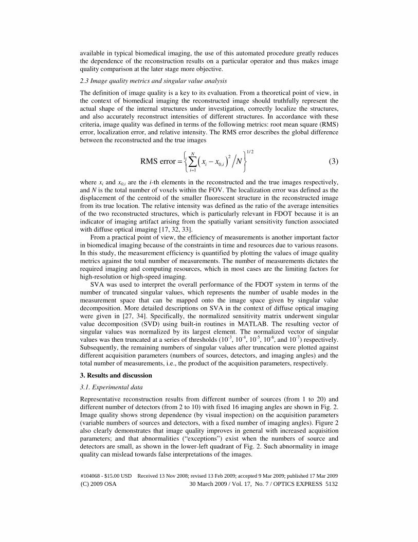
2.3 Image quality metrics and singular value analysis
The definition of image quality is a key to its evaluation. From a theoretical point of view, in
the context of biomedical imaging the reconstructed image should truthfully represent the
actual shape of the internal structures under investigation, correctly localize the structures,
and also accurately reconstruct intensities of different structures. In accordance with these
criteria, image quality was defined in terms of the following metrics: root mean square (RMS)
error, localization error, and relative intensity. The RMS error describes the global difference
between the reconstructed and the true images
( )1/ 2
2
0,
1
RMS errorN
i i
i
x x N=
= − ∑ (3)
where xi and x0,i are the i-th elements in the reconstructed and the true images respectively,
and N is the total number of voxels within the FOV. The localization error was defined as the
displacement of the centroid of the smaller fluorescent structure in the reconstructed image
from its true location. The relative intensity was defined as the ratio of the average intensities
of the two reconstructed structures, which is particularly relevant in FDOT because it is an
indicator of imaging artifact arising from the spatially variant sensitivity function associated
with diffuse optical imaging [17, 32, 33].
From a practical point of view, the efficiency of measurements is another important factor
in biomedical imaging because of the constraints in time and resources due to various reasons.
In this study, the measurement efficiency is quantified by plotting the values of image quality
metrics against the total number of measurements. The number of measurements dictates the
required imaging and computing resources, which in most cases are the limiting factors for
high-resolution or high-speed imaging.
SVA was used to interpret the overall performance of the FDOT system in terms of the
number of truncated singular values, which represents the number of usable modes in the
measurement space that can be mapped onto the image space given by singular value
decomposition. More detailed descriptions on SVA in the context of diffuse optical imaging
were given in [27, 34]. Specifically, the normalized sensitivity matrix underwent singular
value decomposition (SVD) using built-in routines in MATLAB. The resulting vector of
singular values was normalized by its largest element. The normalized vector of singular
values was then truncated at a series of thresholds (10-3
, 10-4
, 10-5
, 10-6
, and 10-7
) respectively.
Subsequently, the remaining numbers of singular values after truncation were plotted against
different acquisition parameters (numbers of sources, detectors, and imaging angles) and the
total number of measurements, i.e., the product of the acquisition parameters, respectively.
3. Results and discussion
3.1. Experimental data
Representative reconstruction results from different number of sources (from 1 to 20) and
different number of detectors (from 2 to 10) with fixed 16 imaging angles are shown in Fig. 2.
Image quality shows strong dependence (by visual inspection) on the acquisition parameters
(variable numbers of sources and detectors, with a fixed number of imaging angles). Figure 2
also clearly demonstrates that image quality improves in general with increased acquisition
parameters; and that abnormalities (“exceptions”) exist when the numbers of source and
detectors are small, as shown in the lower-left quadrant of Fig. 2. Such abnormality in image
quality can mislead towards false interpretations of the images.
#104068 - $15.00 USD Received 13 Nov 2008; revised 13 Feb 2009; accepted 9 Mar 2009; published 17 Mar 2009
(C) 2009 OSA 30 March 2009 / Vol. 17, No. 7 / OPTICS EXPRESS 5132
In Fig. 3, image quality metrics are plotted against the number of sources, the number of
detectors, and the number of imaging angles (from left to right) for the study cases listed in
Table 2. For RMS and localization errors, as shown in Figs. 3(a) and 3(b), respectively, a
smaller value indicates better image quality. For relative intensity, shown in Fig. 3(c),
however, a value closer to unity represents better image quality. In these plots, the curves of
image quality metrics either monotonically improve or severely oscillate before they
eventually stabilize to a certain level. Although the total number of measurements can differ
significantly in different cases, for example, comparing Case 1 with Case 2 or 3, the values of
all image quality metrics stabilize after the acquisition parameters are greater than certain
critical values: ~5 for the number of sources, ~15 for detectors, and ~20 for imaging angles,
as marked by broken lines in Figs. 3(a)-3(c). Note that these critical values remain virtually
the same even though other parameters have changed, as shown in Fig. 3(a1) in particular.
This might seem to contradict the conventional belief that more measurement would result in
better image quality. In fact, as further proven using SVA, this phenomenon reflects the
differences in measurement efficiencies of different acquisition parameters.
To better illustrate the differences in measurement efficiency, the same image quality
metrics are plotted against the total number of measurements, which is the product of the
numbers of sources, detectors, and angles, for all study cases, as shown in Figs. 3(d)-3(f). We
define the criteria of finding higher measurement efficiency for different acquisition
parameters as “obtaining the same image quality with a smaller number of measurements,” or
equivalently as “obtaining a better image quality with the same number of measurements.”
Using these criteria, Fig. 3(d1) suggests that the increase in the number of sources is the most
efficient way to lower RMS errors. Indeed, doubling either the number of detectors or angles
does not reduce RMS error, although the number of measurements has been doubled for the
Fig. 2. Comparison of reconstructed images (23×23 pixels FOV with 1 mm/pixel) using
different numbers of sources and detectors (fixed 16 imaging angles). In the true image, the
upper area is the smaller fluorescent structure (3 mm diameter); and the lower one is the larger
structure (4 mm).
True
image
2 4 6 8
1
2
4
6
8
10
20
10
Number of detectors
Nu
mb
er o
f so
urc
es
#104068 - $15.00 USD Received 13 Nov 2008; revised 13 Feb 2009; accepted 9 Mar 2009; published 17 Mar 2009
(C) 2009 OSA 30 March 2009 / Vol. 17, No. 7 / OPTICS EXPRESS 5133
Number of sources
RM
S e
rro
r
Fig. 3. Image quality metrics derived from experimental data in terms of (a) RMS error, (b)
localization error, and (c) relative intensity in different study cases, from left to right: variable
number of sources (Cases 1 to 3), detectors (Cases 4 to 6), and imaging angles (Cases 7 to 9).
The bottom rows (d-f) are derived from the same data as in (a-c) but are plotted against the
number of measurements.
Loca
liza
tio
n e
rror
(mm
) R
ela
tive
inte
nsi
ty
Number of detectors Number of angles
Variable num. of sources Variable num. of detectors Variable num. of angles
0 5 10 15 20 254
5
6
7
8
9
10x 10
-4
0 20 40 60 80 100 120 140 160 1801804
5
6
7
8
9
10x 10
-4
0 5 10 15 20 25 304
5
6
7
8
9
10x 10
-4
0 5 10 15 20 250.9
1
1.1
1.2
1.3
1.41.4
0 5 10 15 20 25 300.9
1
1.1
1.2
1.3
1.4
0 20 40 60 80 100 120 140 160 1800.9
1
1.1
1.2
1.3
1.4
0 20 40 60 80 100 120 140 160 1800
2
4
6
8
10
12
0 5 10 15 20 25 300
2
4
6
8
10
12
0 5 10 15 20 250
2
4
6
8
10
12
(1) (2) (3)
(a)
(b)
(c)
Number of measurements
0 2000 4000 6000 8000 10000 120000
2
4
6
8
10
12
0 2000 4000 6000 8000 10000 120000
2
4
6
8
10
12
0 2000 4000 6000 8000 10000 120000
2
4
6
8
10
12
Loca
liza
tio
n e
rror
(mm
)
(e)
0 2000 4000 6000 8000 10000 120000.9
1
1.1
1.2
1.3
1.4
0 2000 4000 6000 8000 10000 120000.9
1
1.1
1.2
1.3
1.4
0 2000 4000 6000 8000 10000 120000.9
1
1.1
1.2
1.3
1.4
Rel
ati
ve
inte
nsi
ty
(f)
(d)
0 2000 4000 6000 8000 10000 120004
5
6
7
8
9
10x 10
-4
0 2000 4000 6000 8000 10000 120004
5
6
7
8
9
10x 10
-4
0 2000 4000 6000 8000 10000 120004
5
6
7
8
9
10x 10
-4
RM
S e
rro
r Case 7
Case 8
Case 9
Case 4
Case 5
Case 6
Case 1
Case 2
Case 3
#104068 - $15.00 USD Received 13 Nov 2008; revised 13 Feb 2009; accepted 9 Mar 2009; published 17 Mar 2009
(C) 2009 OSA 30 March 2009 / Vol. 17, No. 7 / OPTICS EXPRESS 5134
same number of sources (Cases 2 and 3 compared to Case 1). From Fig. 3(d2), one can draw
the conclusion that increasing the number of sources is more efficient that the number of
detectors, which is subsequently more efficient than the number of angles, because for the
same number of measurements, doubling the number of sources (Case 5) gives a smaller RMS
error, while doubling the number of angles (Case 6) results in a larger RMS error. Figure 3(d3)
shows that doubling the number of sources (Case 8) reduces the RMS error. Overall, Figs.
3(d1)-3(d3) consistently demonstrate that for our experimental configuration and reasonably
close to the chosen values of acquisition parameters, increasing the number of sources is more
efficient than the number of detectors, which is in turn is more efficient than increasing the
number of imaging angles. The same conclusion can be drawn using the localization error and
relative intensity, as shown in Figs. 3(e) and 3(f), respectively. It is relatively less definitive to
use localization error to determine the order of efficiency because its stabilized value reaches
sub-millimeter levels, which are less than the voxel size in image reconstruction, and thus
makes comparison relatively difficult.
3.2. Singular value analysis
The SVA results for different sampling strategies (Cases 1-9 listed in Table 2) are shown in
Fig. 4. In the top row, the NSV above a series of thresholds (10-3
, 10-4
, till 10-7
) are plotted
against the number of sources, the number of detectors, and the number of imaging angles, as
shown in Fig. 4(a), which corresponds to Cases 1, 4, and 7, respectively. In these plots, the
behavior of each curve is noticeably different from each other with respect to different
acquisition parameters: the amplitudes that the curves reach and their linearity, for example.
The difference is more prominent when the threshold is relatively small (starting from 10-5
,
but 10-6
and 10-7
in particular).
We compared the critical values observed from the experimental data and SVA, at which
the improvement of image quality and the increment rate of the NSV curves change
significantly, and found that the threshold of 10-5
in SVA best characterize our experimental
data, as shown in Fig. 4(b). In each of these plots, a NSV curve initially increases rapidly and
eventually reaches a plateau. The transition between these two stages is the “critical value” of
the corresponding acquisition parameter in our FDOT system because it is around this point
when the increment rate of NSV starts to decrease dramatically. It is interesting to notice the
similarity between the NSV curves with different acquisition constants, i.e., comparing curves
for Cases 1 through 3, 4 through 6, and 7 through 9. The critical values remain virtually the
same even though other constant parameters have been doubled—the same conclusion drawn
from the experimental data (~5 sources, ~15 detectors, and ~20 angles, as marked by broken
lines in Fig. 3). The shapes of the NSV curves are also consistent with our experimental
results. For example, the transition of the NSV curves using variable number of detectors is
more gradual than those of the other two parameters, i.e., Fig. 4(b2) compared to Figs. 4(b1)
and 4(b3), which results in less significant changes in image quality (from experimental data)
before and after the critical values with variable number of detectors then the other two
acquisition parameters, i.e., Figs. 3(a2)-3(c2) compared to Figs. 3(a1)-3(c1) and Figs. 3(a3)-
3(c3). As expected, when the constant acquisition parameters were doubled, the NSV curves
(green and blue) are in general higher than the original curves (red).
When the NSV are plotted against the number of measurements, the red curve can be on
top of, in between, or beneath the green and blue curves, as shown in Fig. 4(c), which clearly
indicates the relative measurement efficiencies of different acquisition parameters. More
specifically, because doubling the number of detectors and angles does not increase the NSV
for variable number of sources, as shown in Fig. 4(c1); because doubling the number of
sources increases the NSV, while doubling the number of angles not, for variable number of
detectors, Fig. 4(c2); and because doubling the number of sources and detectors both increase
the NSV for variable number of angles, Fig. 4(c3), it can be concluded that with a threshold of
10-5
, increasing the number of sources is more efficient in improving NSV than the number of
#104068 - $15.00 USD Received 13 Nov 2008; revised 13 Feb 2009; accepted 9 Mar 2009; published 17 Mar 2009
(C) 2009 OSA 30 March 2009 / Vol. 17, No. 7 / OPTICS EXPRESS 5135
detectors, which in turn is more efficient than the number of angles. This conclusion is
identical to the one drawn from our experimental data. We note that an increase in the NSV is
always desirable.
(a)
Variable num. of sources
Fig. 4. (a) and (b) Comparison of the NSV against variable acquisition parameters and (c)-(e)
the number of measurements using different thresholds in SVA in each of the study cases, from
left to right: variable number of sources (Cases 1 to 3), number of detectors (Cases 4 to 6), and
number of angles (Cases 7 to 9). All of the vertical axes represent the NSV, although their
scales are different among different rows. The horizontal axes in (a) and (b) are the number of
source, the number of detectors, and the number of angles (left to right, respectively); and
those in (c)-(e) are the number of measurements.
0 2000 4000 6000 8000 10000 120000
100
200
300
400
500
600
700
800
0 2000 4000 6000 8000 10000 120000
100
200
300
400
500
600
700
800
0 2000 4000 6000 8000 10000 120000
100
200
300
400
500
600
700
800
Nu
m. o
f si
ng
ula
r va
lues
Number of sources
Variable num. of detectors Variable num. of angles
Number of measurements
Number of detectors Number of angles
0 2000 4000 6000 8000 10000 120000
50
100
150
200
250
0 2000 4000 6000 8000 10000 120000
50
100
150
200
250
0 2000 4000 6000 8000 10000 120000
50
100
150
200
250
0 2000 4000 6000 8000 10000 120000
500
1000
1500
2000
2500
3000
0 2000 4000 6000 8000 10000 120000
500
1000
1500
2000
2500
3000
0 2000 4000 6000 8000 10000 120000
500
1000
1500
2000
2500
3000
Case 1
Case 2
Case 3
Case 4
Case 5
Case 6
Case 7
Case 8
Case 9
SV
A t
hre
shold
= 1
0-6
S
VA
th
resh
old
= 1
0-4
S
VA
th
resh
old
= 1
0-5
M
ult
iple
SV
A t
hre
sho
lds
(b)
(c)
(d)
(e)
0 20 40 60 80 100 120 140 160 1800
100
200
300
400
500
600
700
800
0 5 10 15 20 25 300
100
200
300
400
500
600
700
800
0 5 10 15 20 250
100
200
300
400
500
600
700
800
0 5 10 15 20 250
500
1000
1500
2000
2500
3000
3500
4000
4500
10-3
10-4
10-5
10-6
10-7
0 5 10 15 20 25 300
500
1000
1500
2000
2500
3000
3500
4000
4500
0 20 40 60 80 100 120 140 160 1800
500
1000
1500
2000
2500
3000
3500
4000
4500
10-7
10-4 10-5
10-6
10-3
(1) (2) (3)
#104068 - $15.00 USD Received 13 Nov 2008; revised 13 Feb 2009; accepted 9 Mar 2009; published 17 Mar 2009
(C) 2009 OSA 30 March 2009 / Vol. 17, No. 7 / OPTICS EXPRESS 5136
However, if using a larger threshold, e.g., 10-4
, the relative order of measurement
efficiency changes to: increasing the numbers of sources or angles is equally more efficient
than the number of detectors, as shown in Fig. 4(d). Using a threshold of 10-3
gives the same
result (data not shown). Using a smaller threshold, e.g. 10-6
, shown in Fig. 4(e), and 10-7
(data
not shown), the relative efficiencies of acquisition parameters are the same as using the
threshold of 10-5
, except that the differences between the acquisition parameters are less
significant and the overall trend of the NSV curves resembles closer to a straight line, which
occurs when the threshold is zero.
In this study, the overall performance of our FDOT system was characterized by a
threshold of 10-5
used in SVA. The effect of sampling strategies on image quality was
compared in terms of a number of image quality metrics for reconstruction results and in
terms of the NSV in a more generalized SVA. The results are representative for similar
noncontact FDOT systems, such as [19], and can be used to assist the choice of acquisition
parameters in experimental designs—a tradeoff between image quality and resources.
The NSV curves are, in general, consistent with the image quality metrics defined in this
study. Nonetheless, a larger NSV does not necessarily translate into a higher score in every
metric. This is because a particular image quality metric represents only one characteristic of
a complex imaging system, which consists of imaging apparatus and reconstruction methods.
On the other hand, differences due to specific imaging hardware, experimental configurations,
and reconstruction methods can alter the outcome of the analysis. This study adopted a way to
characterize the overall performance of an imaging system in terms of the threshold in SVA.
With the same imaging apparatus and similar experimental configurations, this threshold can
be used to predict outcomes of FDOT imaging using other sampling strategies. With this
method, a more generalized analysis of sampling strategies can be conducted with more
acquisition parameters, for example, the 2-D distribution of sampling points for sources and
detectors, as well as angular coverage and distribution of imaging angles. The effect of
experimental configuration, e.g., relative angular positions of the scanning laser and the
camera, on the characteristic SVA threshold and further on image quality can be investigated
using this approach as well, which is beyond the scope of this study.
It is important to point out that this study has been purposefully limited to 2-D on a
limited imaging parameters, although FDOT is fundamentally a 3-D imaging method. This is
primarily because the image quality is affected by so many parameters that it would be
impractical to cover the full effects of all possible imaging parameters and experimental
configurations in this study. Instead, we focused only on the most fundamental imaging
parameters that are pertinent to the majority of FDOT experiments. For the same reason, the
phantom design and image analysis were limited to 2-D as well in order to avoid being too
specific on particular image processing algorithms and to avoid the complexity of image
analysis in 3-D.
4. Conclusions
The effects of sampling strategy on image quality were studied using a noncontact panoramic
FDOT system in an imaging phantom for small animals. The aim was to guide the choice of
acquisition parameters for a given imaging system and a reconstruction method to optimize
imaging quality, while minimizing measurement and computation time. We found that critical
values for acquisition parameters exist, beyond which image quality improves at a much
slower rate. These critical values largely remain the same despite significant change of other
acquisition parameters. We also found that the improvement of imaging quality due to
increased acquisition parameters varies not only based on the specific parameter, but also on
the overall characteristic of the imaging system. In terms of the number of measurements,
increasing the number of sources is more efficient in improving image quality than the
number of detectors and subsequently the number of angles, if the SVA threshold is small
(less than or equal to 10-5
using our imaging system); or the number of sources and the
#104068 - $15.00 USD Received 13 Nov 2008; revised 13 Feb 2009; accepted 9 Mar 2009; published 17 Mar 2009
(C) 2009 OSA 30 March 2009 / Vol. 17, No. 7 / OPTICS EXPRESS 5137
number of imaging angles are almost equally more efficient than the number of detectors, if
the SVA threshold is large (greater or equal to 10-4
in our study). The results presented in this
article clearly show that a well-designed experiment based on the characteristics of the FDOT
system can significantly improve imaging quality and/or reduce acquisition and computing
time. Extensions of this study are under way to investigate generalized optimal imaging
strategies in full 3-D phantom setups, which incorporate more sophisticated modeling
techniques, allow more degrees of freedom, and include more acquisition parameters.
Acknowledgment
This study was funded by NIH/NCRR P41 RR005959 and NCI SAIRP U24 CA092656. The
authors are grateful to Professor G. Allan Johnson for his mentorship and to Sally Zimney for
her assistance in editing.
#104068 - $15.00 USD Received 13 Nov 2008; revised 13 Feb 2009; accepted 9 Mar 2009; published 17 Mar 2009
(C) 2009 OSA 30 March 2009 / Vol. 17, No. 7 / OPTICS EXPRESS 5138