REPORT NO. UCB/EERC-89/06 JULY 1989 PB91-229161 EARTHQUAKE ENGINEERING RESEARCH CENTER EFFECTS OF SPATIAL VARIATION OF GROUND MOTIONS ON LARGE MULTIPLY-SUPPORTED STRUCTURES by HONG HAO PREFACE by BRUCE A. BOLT and JOSEPH PENZIEN COLLEGE OF ENGINEERING UNIVERSITY OF CALIFORNIA AT BERKELEY REI"RODUCED BY U.S. DEPARTMENT OF COMMERCE NATIONAL TECHNICAL INFORMATION SERVICE SPRINGFIELD, VA 22161
Transcript
REPORT NO.
UCB/EERC-89/06
JULY 1989
-----~'
PB91-229161
EARTHQUAKE ENGINEERING RESEARCH CENTER
EFFECTS OF SPATIAL VARIATIONOF GROUND MOTIONS ON LARGEMULTIPLY-SUPPORTED STRUCTURESby
HONG HAO
PREFACE
by
BRUCE A. BOLT
and
JOSEPH PENZIEN
COLLEGE OF ENGINEERING
UNIVERSITY OF CALIFORNIA AT BERKELEYREI"RODUCED BYU.S. DEPARTMENT OF COMMERCE
NATIONAL TECHNICALINFORMATION SERVICESPRINGFIELD, VA 22161
I.b
For sale by the National Technical InformationService, U.S. Department of Commerce,Springfield, Virginia 22161
See back of report for up to date listing ofEERC reports.
DISCLAIMERAny opinions, findings, and conclusions orrecommendations expressed in this publication are those of the authors and do not necessarily reflect the views of the National Science Foundation or the Earthquake Engineering Research Center, University of Californiaat Berkeley.
EFFECTS OF SPATIAL VARIATION OF GROUND MOTIONS
ON LARGE MULTIPLY-SUPPORTED STRUCTURES
by
Hong Hao
PREFACE
by
Bruce A. Boltand
Joseph Penzien
Report to the National Science Foundation
Report No. UCB/EERC-89/06
Earthquake Engineering Research Center
University of California
Berkeley, California
July 1989
,J. a-
PREFACE
This is the fourth report III a research series which is based on measurements made
of seismic strong ground motion by the large-scale digital array of accelerometers in Taiwan,
called SMART-I. The array was installed and is operated by the Institute of Earth Sciences
and National Science Council, Taiwan, R.O.C.. The uniformly diligent work carried out by
scientists at the Institute has provided high-quality data for many studies. SMART-1 began
operation in September 1980 and through June 1989 recorded strong ground motions (with
some accelerations exceeding 0.3g) from over 50 local earthquakes. The first two reports in
the series are: UCB/EERC-82/18 by B. A. Bolt, C. H. Loh, J. Penzien, Y. B. Tsai and
Y. T. Yeh and UCB/EERC-85/82 by N. A. Abrahamson. In 1988, R. B. Darragh published
"Analysis of Near Source Waves: Separation of Wave Types Using Strong Motion Array
Recordings" in Report UCB/EERC-88/o8. A research Summary through 1986 was published
III "Earthquake Spectra", ~, 263-287, 1987 by N. A. Abrahamson, B. A. Bolt, R. B. Darragh,
J. Penzien and Y. B. Tsai.
From its inception, the SMART-1 research program has had as a major goal the
accumulation of ground motion data which were useful in exploring the effect of seismic in
puts on multiply-supported large structures. For theoretical reasons, it was expected that
multiple-inpu t effects could not be represented adequately by a single base excitation because
of phase differences and loss of wave coherency. For dynamical analysis of large structures for
earthquake resistance, inclusion of multiple-inputs might well be envisaged in certain circum
stances. Over the last several years, earthquake engineers around the world have made use
of SMART-l data to explore aspects of this problem, particularly that related to incoherency
in strong ground motion over distances of order 100 meters. This work has led, among other
results, to the construction of various coherency models of wave propagation as functions of
separation distance of the supports and of the frequency.
The present report by Dr. Hong Hao advances the study of the effects of the spatial
variation of ground motions on large multiply-supported structures. He has applied random
processes to develop particular simulation techniques that generate multiple-support inputs
which allow more realistic assessment of structural response than the usual present practice.
His main conclusions bear on two aspects of the problem. The first is the simulation of
realistic ground motion for spatially-correlated, quasi-stationary multiple ground motions and
the second is the development of an appropriate computer program which would simulate
structural response itself, including soil-structure interaction effects. He has suggested a model
for coherency with four parameters and has explored the nonlinear interaction between the
parameters. The models have been tested using earthquakes recorded by SMART-I. In his
second main contribution, Dr. Hong Hao has developed ways to interpolate multiple-motion
time histories to preserve the properties of the prescribed ground motion and response spectra.
His newly-written computer program demonstrates that often there is a general reduction in
structural response when multiple inputs are used and that response modes such as rocking
and rotation are significant when different phasing is allowed at each input.
The report uses methods of array analysis not ordinarily available in the engineering
literature. For a basic explanation of these methods, readers are referred to "Seismic Strong
Motion Synthetics," B. A. Bolt (Editor), Academic Press, 1987.
B. A. Bolt
J. Penzien
11
ABSTRACT
The spatial variability of ground motions recorded during 17 earthquakes by a strong
motion accelerograph array in Taiwan (SMART-I) is analyzed. The power spectral density
functions and envelope functions of the ground motion are calculated and compared with
previous results. A coherency function is suggested for pairs of stations as a function of
both frequency and also the projected separation distances between the stations in the wave
propagation and transverse directions, respectively. The apparent velocities of the seismic
waves are studied in different time windows as a function of frequency. A method is developed
to simulate and interpolate multiple ground motions that are spatially correlated, quasi
stationary, and response spectrum compatible. Also, the equations that describe structural
response under multiple ground motion excitations are formulated in the cases both with and
without soil-structure interaction effects. Numerical methods for solving these equations in
the frequency domain are presented.
A computer program SSIAM is developed. It can simulate and interpolate spatially cor
related, stationary or quasi-stationary multiple ground motions compatible with the prescribed
ground motion properties and the given response spectrum. It then uses these simulated
ground motions as the multiple inputs to solve the structural responses. By using program
SSIAM, some examples of ground motion simulation and interpolation are calculated. The
results are presented and compared with the prescribed ground motion properties; also, some
examples of structural responses under the simulated multiple ground motion excitations are
calculated with soil-structure interaction effects. The results show that it is important to
consider the ground motion wave propagation effects in seismic response analysis of large
dimensional structures.
111
ACKNOWLEDGEMENTS
I am grateful to Professors Joseph Penzien and Bruce A. Bolt, who kindly guided me
throughout the course of this work, and offered encouragement and many valuable suggestions
and insights.
Thanks also go to Dr. Carlos S. Oliveira, Earthquake Engineering Instituto Superior
Tecnico, Lisbon, Portugal, for valuable discussions during his periodical visits to Berkeley,
and to Mr. S. J. Chiou for providing me with the recorded earthquake data. Also, thanks
to Dr. Beverley Bolt for editing this report.
Part of my study and research at Berkeley was supported by the Ministry of Education
of the People's Republic of China and National Science Foundation of the U. S. A., and this
support is also acknowledged.
Finally, I would like to extend my deepest gratitude to my family for their continued
support.
IV
TABLE OF CONTENTS
Preface
Abstract
Acknowledgements
Table of Contents
1 INTRODUCTION
2 NUMERICAL PROCESSING METHODS FOR RANDOM PROCESSES
2.1 Estimation of Covariance .
2.2 Estimation of Spectra, Coherency and Phase Spectrum
Abrahamson and Darragh (1987) have used the triangular shape window m the fre
quency domain. The inverse Fourier transform of this window is given by
(2.10)
4
(2.11)
which can be used to smooth the covariance functiop..
To compute the cross power spectral density function between xdt) and X2(t), both
XI(t) and X2(t) need to be tapered. Then after transforming XI(t) and X2(t) to the frequency
domain, the cross power spectral density function can be obtained using
M
S"""'2(iw) =~ L WmXI(w + 2;m)X;(w + 2;m)m=-M
where X; (w) is the complex conjugate of X 2(w), the Fourier transform of X2 (t) . The co
herency function can now be calculated in accordance with
(2.12)
If uncorrelated nOIse is present in each of Xl (t) and X2 (t), it should be eliminated to
the extent possible by smoothing the power spectra before evaluating the coherency function;
otherwise, significant error will be introduced.
The phase spectrum can be calculated by the following expression
(2.13)
It can be shown that the variance of the smoothed coherency and the phase estimators
depend not only on the type and band width of the spectral window employed, but also on
the coherency. The variances of these estimators are small when the coherency is high, but
increase as the coherency decreases. Noise in the series will tend to dominate when the
coherency values are low; thus, for weakly correlated series, smoothing to remove the noise is
very important. Some researchers also set up confidence levels for coherency by calculating
the numerical coherency values of the noise. Abrahamson (1985) reported 0.4 as a reasonable
coherency confidence level. In the present investigation, the confidence level was found to be
approximately 0.35 at low frequencies, increasing to 0.45 at 10Hz. These are the numerical
coherency values of the white noise after smoothing with a triangular shaped window of width
0.97Hz.
2.3 Estimation of Envelope Function
The envelope function of a time series can be calculated usmg the Hilbert transform
technique. The envelope function le(t) of x(t) is defined as
Ie (t) = x(t) - ilk (t)
5
(2.14)
where fh(t) is the Hilbert transform, which introduces a 900 phase shift with respect to x(t)so that the envelope of the real time function can be obtained. The function fh(t) can be
calculated by the formula,
+00
fh(t) = 2i1l" J[X(iw)e,wt - X(-iw)e-,wt]dw (2.15)
o
and its Fourier transform by
F",(w) = iX(iw)Sgn(w)
where
{
1, w> 0Sgn(w) = 0, w = 0
-1, w < 0
Function fh(t) can now be obtained by applying the inverse FFT to F",(w)j that IS
+00
f",(t) = JFh(w)e,wtdw
-00
Hence the envelope of the time senes x(t) can be obtained by the following formula
(2.16)
(2.17)
(2.18)
(2.19)
A more detailed description of the Hilbert transform theory and its applications can be seen
in Kanasewich (1981).
2.4 Computational Procedures and Examples
The practical procedure of calculating the functions introduced above will now be
outlined and some examples given:
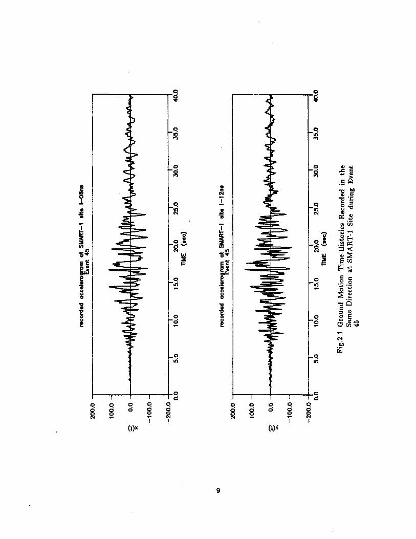
Let us consider the two time senes x(t) and y(t) shown in Fig. 2.1, which are ac
celerograms recorded in the same direction in discrete form at two stations in the SMART-1
array having 400m separation. The recording time increment is 6t = O.Olsee. Assume that
they are samples of stationary processes within the time window 7 - 27see having zero mean
values. Using 6t = O.Olsee, N = 211 = 2048, and T = N 6t = 20.48see, each wave form can
be transformed using the FFT technique. The following steps are followed in calculating the
desired functions:
(a) Covariances, correlations, and envelope functions
1. Reduce each series by its mean value to satisfy the assumption of zero mean
processes.
6
2. Taper the series to make the series compatible with the periodic property
of the FFT requiring that the beginning and the ending values of the series
be continuous.
3. Use Eq.(2.2) to calculate the autocovariance function and Eq.(2.4) to cal
culate the cross covariance function. Then, normalize the autocovariance
function by its value at zero time lag, which yields the autocorrelation coef
ficient function as given by Eq.(2.5). Normalize the cross covariance function
by the product of B",,,,(O) and Byy(O), which gives the cross correlation co
efficient function of Eq.(2.6). Note that the time lag T only needs to be
calculated up to 10 or 20 percent of T. Larger lags will result in unreliable
results since, by shifting the two series away in the convolution process, a
lot of information will be lost.
4. Using the Hilbert transformation technique, the envelope function can be
calculated.
Figure 2.2 shows the autocorrelation coefficient function of x(t). Since this function
IS an even function, it need be evaluated for positive time lags only. Figure 2.3 shows the
cross correlation coefficient function of x(t) and y(t). Unlike the autocorrelation coefficient
function, its peak value equals 0.769, which does not occur at zero lag but at T = 0.07sec.
For the wave propagation problem, this means that the dominant waves travel from the point
of measuring x(t) to the point of measuring y(t) in 0.07sec. This information which is very
important in studying the spatial variation of ground motion, can be used to calculate the
apparent wave velocity. This velocity is calculated by dividing the projected distance along
the main wave propagation direction by T. Figures 2.4 and 2.5 show envelope functions of
x(t) and y(t), respectively.
(b) Power spectrum, coherency and phase spectrum
1. Remove the mean and taper of the sample wave forms.
2. Compute the Fourier transform of each wave form
3. Filter the wave forms in the frequency domain. If the wave forms are
represented by frequencies higher than the Nyquist frequency In = 1/(26t),
the power spectrum will be aliased into a power spectrum represented only
in the principal range [-In, In]' In this case, the wave forms should be
filtered to remove the power at frequencies above In' Also, for practical
reasons, the power below a selected frequency should be removed.
7
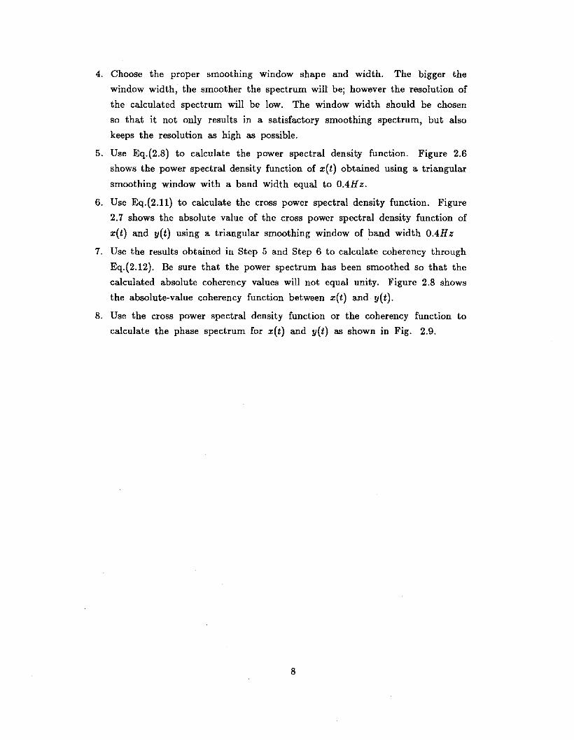
4. Choose the proper smoothing window shape and width. The bigger the
window width, the smoother the spectrum will be; however the resolution of
the calculated spectrum will be low. The window width should be chosen
so that it not only results in a satisfactory smoothing spectrum, but also
keeps the resolution as high as possible.
5. Use Eq.(2.8) to calculate the power spectral density function. Figure 2.6
shows the power spectral density function of x(t) obtained using a triangular
smoothing window with a band width equal to OAHz.
6. Use Eq.(2.11) to calculate the cross power spectral density function. Figure
2.7 shows the absolute value of the cross power spectral density function of
x(t) and y(t) using a triangular smoothing window of band width OAHz
7. Use the results obtained in Step 5 and Step 6 to calculate coherency through
Eq.(2.12). Be sure that the power spectrum has been smoothed so that the
calculated absolute coherency values will not equal unity. Figure 2.8 shows
the absolute-value coherency function between x(t) and y(t).
8. Use the cross power spectral density function or the coherency function to
calculate the phase spectrum for x(t) and y(t) as shown in Fig. 2.9.
8
reco
rded
acce
lero
gram
at
SMAR
T-1
alte
1-08
nBE
vent
45
40.0
35
.0JO
.O2
5.0
15.0
20.0
nME
(Bee
)10
.05.
0
200.
0I
i
100.
0
-20
0.0
II
II
1I
1I
I0
.0
-10
0.0
~0
.01
•Ie.~mnAfV\"'V'"
..111
11\1
11,
.II~
,1\I
V'"
AfU
T\.
.....J
HvP
.:MI
"N"V
V\
?DA
-.1
~)(
tore
cord
edac
cele
rogr
ama
tSM
ART-
1II
lte1-
12nB
Eve
nt45
200.
0i
i
100.
0
80.
0I
......
.,#4JJr~"""1
>..
-10
0.0
40.0
25.0
15.0
20.0
TlN
E(B
ee)
10.0
5.0
-20
0.0
fI
II
II
II
I0
.0
Fig
.2.1
Gro
und
Mot
ion
Tim
e-H
isto
ries
Rec
orde
din
the
Sam
eD
irec
tion
atS
MA
RT
-lS
ite
duri
ngE
vent
45
5.04.02.0 3.0nUE (••e)
1.0
1.0 ..,...-----------------------,
0.8
0.6
0.48)( 0.2
S 0.0 ~+--..,..._-...,.....~~f---'Ir___+_----''t_-=_-_+__l
i1-0•2
8 -0.4
1-0.6
-0.8
-1.0 -+----~----r_---"T""'---_r---~0.0
Fig.2.2 Autocorrelation Coefficient Function of x(t)
When ground motions are simulated for engineering design purposes, they should be re
alistic representations of the seismic motions expected at the site under consideration. Hence,
it is necessary to know such properties of the expected ground motion as duration, peak,
shape function, power spectral density function, coherency, and apparent velocity. Knowing
these ground motion properties, one can generate realistic inputs to be used in dynamic anal
yses; and thus, contribute to the design of economical and safe structures. In this chapter,
the recorded SMART-1 ground motions of two earthquake events are analyzed to establish
shape functions, power spectral density functions, and apparent wave velocities with respect
to different frequencies. Also, the ground motions are analyzed to establish a coherency func
tion which can be used in simulating spatial variation of the ground motions. While these
functions are site specific for the SMART-1 site, they can also be used for sites with similar
properties.
3.1 The SMART-1 Array
The SMART-1 array, see Bolt, et al. (1982) and Darragh (1987), is the first high
density array developed that permits the study of spatial variation of ground motion in
a small area. The array is located in the northeast corner of Taiwan near the city of
Lotung on the Lan-yang plain; see Fig. 3.1. The array consists of 37 force-balanced triaxial
accelerometers configured in three circular concentric rings of radii 200m, lOOOm, and 2000m.
The three rings are named I(inner), M(middle) , and O(outer) , respectively. There are 12
stations in each ring named from 1 to 12, and one center station named C-OO. The distance
between station pairs varies from a minimum of approximately 105m to a maximum of 4000m.
In June 1983, two additional stations, E-01 and E-02, were added to the array at 2.8km and
4.8km south of the center station. The configuration of the array is shown in Fig. 3.2.
The SMART-1 array is located on recent alluvium. The ground water level is almost
at ground surface. The area is very flat having surface elevations which vary from 204m
to 18.1m. All stations are located on soil sites, except for station E-02 which is located on
rock. Two north-south cross sections are shown in Fig. 3.3. The soils beneath the main array
consist of 4-12 meters of clays and muds over recent alluvium of depths up to 50m. Below
the alluvium layer are gravels having pebble sizes which increase with depth. The bedrock
below the gravels is slate. The depth of the bedrock varies from 170m at the southern end
of the outer ring to 600m at the northern end of the outer ring. The foundation properties
and the P and S wave velocities are given in Table 3.1. These data were obtained by the
HCK Geophysical Company by drilling seven holes and using crosshole and uphole seismic
14
methods.
3.2 Information Recorded by the SMART-l Array
This array recorded its first earthquake on October 18, 1980. Up to January~ 1988, 50
events had been recorded by some or all stations in the array. Figure 3.4 shows the epicentral
positions of the seventeen recorded events used in this study. Among all these events, Events
24 and 45 were chosen to be studied thoroughly for power spectral density functions, envelope
functions, apparent velocities, and coherency because of their long epicentral distances and
high magnitudes. Figure 3.5 shows some of the recorded accelerograms of Event 24. Besides
completely processing the recorded accelerograms of Events 24 and 45, a total of seventeen
events were chosen to be studied intensively for coherency effects. Special study is needed
since coherency is the most important function characterizing spatial variations of ground
motion. The seventeen earthquakes chosen were selected on the basis of having epicentral
distances larger than 30km, magnitudes larger than 5, and having triggered at least seven of
the inner ring stations. Table 3.2 gives information on each of these events.
3.3 Power Spectral Density Function
The power spectral density function is a measure of the frequency content in a station
ary random process. Earthquake ground motions are actually nonstationary in both the time
and frequency domains. It is found, however, that a satisfactory and practical way of treating
ground motion nonstationarity, is to assume the ground motions to be piecewise stationary or
quasi-stationary. This assumption is made on the basis that ground motions propagating in
the earth usually consist of three different types of wave; the primary P-wave, the secondary
S-wave, and surface waves (Rayleigh and Love waves). The motions of each wave type can
be modelled as a stationary process better than the combined motions of all the wave types.
The piecewise stationary assumption is applied in the subsequent treatment.
Power spectral density functions were calculated for all components of ground motion
recorded at the inner ring stations for Events 24 and 45 using the frequency domain method
given in the previous chapter, Eq.(2.8). Triangular smoothing windows were used for all
the calculations using the data of Events 24 and 45. The window width and M-value were
chosen such that the resulting power spectral density functions were smooth enough while
their standard deviations were not too large. It was found that the vertical components of
ground motion have higher frequency content and less energy than the horizontal components
for both Events 24 and 45; see Hao (1989). Also, the power spectral density functions for a
particular component are almost the same at all the inner ring stations for each of the two
events, and that the frequency content of the ground motion decreases as the time window
moves to later times.
15
(3.1)
On the basis of the results presented and discussed m Hao (1989) for Events 24 and
45, the following conclusions have been drawn.
1. Attenuation of the ground motion wave propagation can be neglected across
the SMART-1 array, i.e. the intensities of corresponding components of
motion are nearly constant for all stations in the array.
2. The quasi-stationary frequency content assumption can be used to model
the nonstationarity of the ground motion.
3. A power spectral density function of the Tajimi-Kanai form can be satisfac
torily used for simulation purposes.
Thus, power spectral density functions representing the entire site can be obtained by
averaging those for corresponding components of motion recorded throughout the array. This
averaging procedure will greatly reduce the contributions from noise in the resulting power
spectral density functions. Such average results for each component, each time window, and
each event were obtained. The results for the EW components of motion for each of the
two events are shown in Figs. 3.6 through 3.11. These results were used to establish the
Tajimi-Kanai model in each case; the expression for the Tajimi-Kanai form is given by
1 + 4e w:
S(w) = gW g S(1_W2)2+4ew20w; g w;
the corresponding values of Wg, €g, and So were obtained for Events 24 and 45; see Table
3.3.
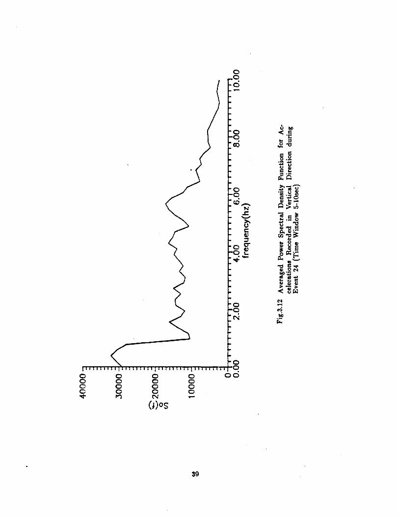
The results for the vertical components of motion for Event 24 are mIssmg m Table
3.3, since it was found that the Tajimi-Kanai model was inadequate. Figure 3.12 shows an
example of the averaged power spectral density function for the vertical component of motion
in the first window as recorded during Event 24. It is seen that the banded white noise
model fits better than the Tajimi-Kanai mod~l in this case. It can be seen that the central
frequency W g decreases with time for all cases except the EW component for Event 24, where
W g actually increases from 1.0Hz to 1.2Hz. The damping ratio €g of the first time window
is much higher than that of the second window. In the first window, eg = 0.95, which
corresponds to a very broad band window. In the second window, €g = 0.3 which represents
a much narrower band.
The above power spectral density function results can be used to simulate ground
motions in consecutive time windows separately. The stationarity assumption can be used
in each time window consistent with the corresponding power spectral density function. The
ground motion mean square intensity in each window can be calculated by integration of the
16
(3.2)
(3.3)
power spectral density function as
q~ = 100
S(w)dw
Substituting the Tajimi-Kanai power spectral density function of Eq.(3.1) into Eq.(3.2) and
integrating gives the covariance of motion in the approximate form
100 1 +4eq~ = S(w)dw = wg g
o 4eg
see Ruiz and Penzien (1969). By using Eq.(3.3) and the parameters in Table 3.3, the normal
ized scale factors for the power spectral density function in each time window are obtained
giving the results presented in Table 3.4. These scale factors for the power spectral density
functions are used to maintain uniform intensity of ground motion within each time window
before applying the time-dependent shape function.
3.4 Shape Function
The shape function is used to characterize ground motion nonstationarity in the time
domain. It is the normalized envelope function of ground motion. Shape functions of all
accelerograms recorded during Events 24 and 45 at the inner ring stations were evaluated
using the Hilbert transform approach described in Chapter 2; see Eq.(2.19). Since there is
no significant attenuation of the ground motions across the array, the shape functions of the
corresponding accelerograms recorded at all inner ring stations can be assumed the same.
Thus, a representative ground motion accelerogram shape function for each component of
motion can be obtained by averaging the shape functions for corresponding accelerograms.
These averaged shape functions for all three components were calculated and plotted. Figures
3.13 and 3.14 show the averaged shape function for the EW component using data from
Events 24 and 45.
It is seen that, except for those generated using the vertical components of motion
recorded during Event 24, all the calculated shape functions of accelerograms are similar to
the Bogdanoff type having the form
t~O
t> 0(3.4)
where a and b are parameters to be determined consistent with observed ground motion
nonstationarity. Figure 3.15 shows the averaged envelope functions for motions recorded in
the vertical direction during Event 24. These shape functions fit better the Amin and Ang
form given by
{
1. (.1.)Zo tlE(t) = f o
foe-c(t-t~)
17
o~ t ~ t 1
t 1 ~ t ~ t zt z ~ t
(3.5)
where 10 represents ground motion intensity., The normalized shape function is obtained by
setting 10 = 1. Quantities t1 , t2 are values of time that separate the shape function into its
parabolic, constant, and exponential decay forms. Constant c controls the rate of decay at
the end of the motion.
To fit the Bogdanoff shape function given by Eq.(3.4), two parameters a and b can be
determined by the condition that at a certain time t = tp, E(t) reaches its peak value which
is normalized to be one. Then, by differentiating Eq.(3.4) with respect to t, one obtains
and
a=~
(3.6)
(3.7)
By solving these two equations for a and b, the shape functions can be determined In terms
of t p and e (the base of the natural logarithm) for all three components motion.
The results for a, b, and t p of Events 24 and 45 are shown in Table 3.5. Since the
results of the vertical component for Event 24 do not fit this type of shape function properly,
values for the above constants are not given in Table 3.5.
3.5 Apparent Velocity
Apparent velocity is one of the most difficult parameters to assess due to the fact that
the waves are of different types moving in different directions experiencing multiple reflections
and refractions.
Some example apparent velocities calculated for Event 45 by the frequency-wave-number
(F-K) method (Abrahamson, 1985) are shown in Fig. 3.16. In this report, the apparent
velocities are assumed to be frequency independent. Thus, by approximately fitting many
F-K results, the apparent velocities of Event 24 are obtained as 3km/s, and 4km/s for the
horizontal and vertical components, respectively, and 4km/sand 6km/s for the apparent
velocity values of Event 45. Two F-K diagrams of the approaching wave field are shown in
Fig. 3.17. From this figure, it is seen that the approaching wave directions are very diverse.
3.6 Coherency
As previously mentioned, coherency is one of the most important and effective quan
tities used to describe the spatial variations of ground motion. Using the SMART-1 data,
several authors have studied the coherency relation given as
( .- d) I (.- d ) I [._Xii]Iii IW, ii = Iii 'IW, ii exp IW-Va
18
(3.8)
where subscripts i and j represent the two different stations, Xii is the projected distance
in the wave propagating direction between stations i and j, Va is apparent velocity, (jj is
circular frequency, and I 'Yii (iw, ~i) I is the loss of coherency with separation due to unknown
effects. All the loss of coherency models, that have been proposed, are dependent only on the
absolute distance between the the two stations; see Loh (1985), Harrichandran and Vanmarcke
(1984), Abrahamson (1988), Tsai (1988), and Loh and Yeh (1988). It has been found that
the loss of coherency is dependent on both the projected distance in the direction of wave
propagation (d~i)' and the projected distance transverse to it (~j) (Hao, 1989).
To develop a new two-dimensional coherency model, the loss of coherency between all
station pairs for all components of ground motion recorded during Events 24 and 45 was
calculated. It has been found that the value~ of loss of coherency were almost the same for
the ground motions recorded in the two horizontal directions, but were different for those
in the vertical direction (Hao, 1989). On the basis of the calculated losses of coherency
for Events 24 and 45, it was found that the coherency model of Eq.(3.8) can still be used
provided it is expressed in the two dimensional form given by
where f is frequency and where d~j and cI;j are the projected longitudinal and transverse
distances defined above. Parameters (31 and f32 are constants which control the coherency
values at zero frequency while Ql (I) and Q2(J) are two frequency dependent parameters
which control the loss of coherency with respect to frequency. All parameters (31, (32, al (I)and Q2(1) were determined by fitting Eq.(3.9) to the coherency data using the least squares
method.
In order to investigate coherency, ground motions recorded during the 17 events shown
m Table 3.2 were used to evaluate f31' f32' Ql (I) and Q2 (I). Since the loss of coherency
with distance can be assumed the same for the two horizontal components of motion, only
the NS components were analyzed. The coherencies of the vertical components were studied
for Events 24 and 45 only.
Loss of coherency values were calculated for all components of motion recorded at the
mner ring station pairs. To aid in interpreting the results, the inner ring station pairs were
divided into 9 groups with respect to the distances d~i and ~i falling in the ranges O-lOOm,
lOO-200m, and 200-400m. All loss of coherency values for station pairs in the same group
were averaged. These average values were then considered to represent the loss of coherency
for d~j and ~j at distances of 50m, 150m, and 300m.
The two constant parameters f31 and f32 were determined using the loss of coherency
19
values at -zero frequency for each of the 9 distance groups for each event. The detailed
procedure can be seen in Hao (1989); the results are presented in Table 3.6 for all 17 events.
To calculate the two frequency parameter functions al (J) and a2 (J) for each event,
the least squares method was used. It was found that two nonlinear functions
aad/) = I + bf + c
da2 (J) = I + ef + 9
(3.1O)
best fit the raw data, where a, b, c, d, e, and 9 are SIX constants, which were obtained
by weighted least squares fitting. The values of the six constants obtained for all 17 events,
which are valid for 0.05Hz ~ f ~ 10Hz and 0 ~ dL·, ~j ~400m, are presented in Table
3.7. When f > 10Hz, the loss of coherency values can be assumed to be constant at the
f = 10Hz value. The detailed procedure can be found in Hao (1989).
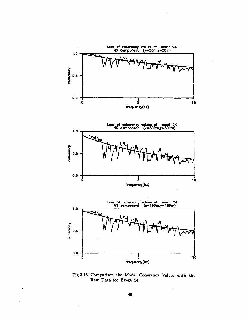
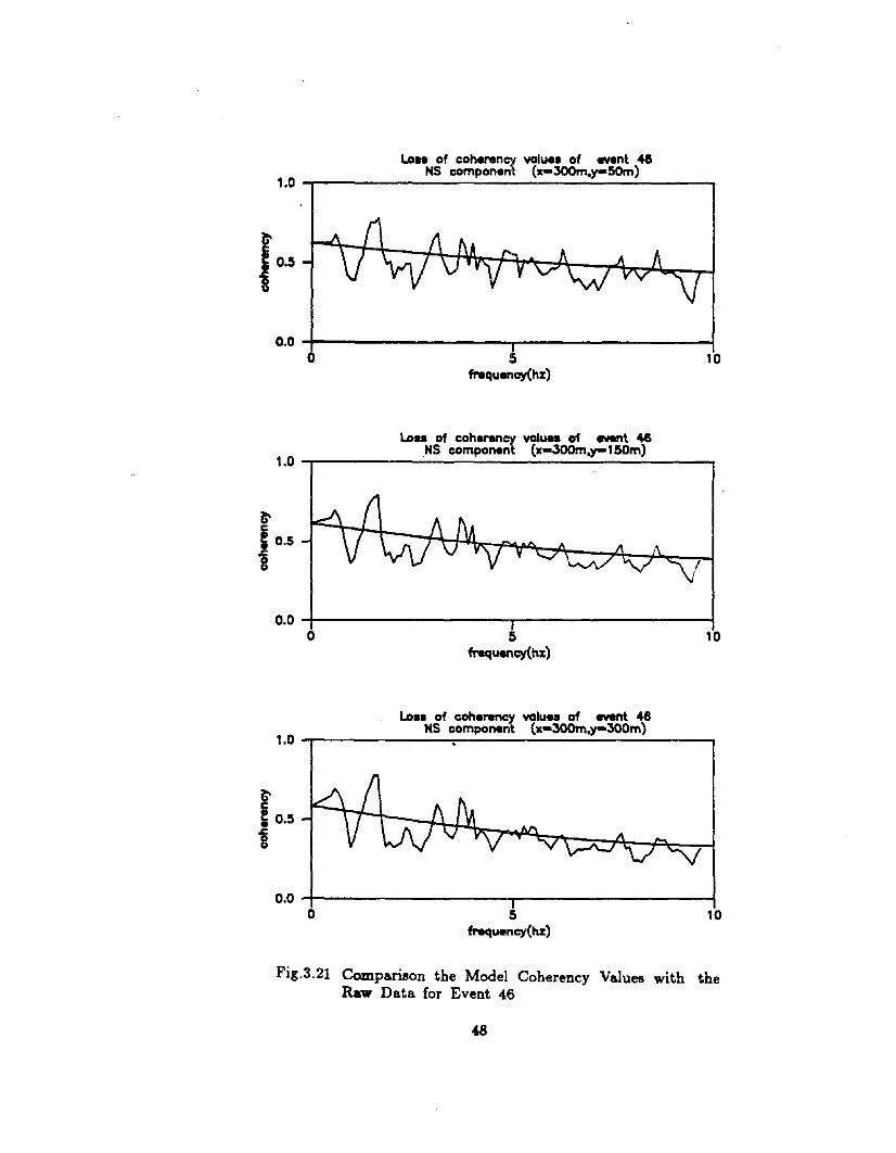
Figures 3.18 through 3.21 show comparisons between the loss of coherency values cal
culated by Eq.{3.9) and the generated values using the raw data for Events 24, 31, 45, and
46. Similar comparisons were found using the data for all 17 events. From these figures, it
can be noticed that, at the lower frequencies, the analytical model values are always smaller
than those generated directly from the raw data. Also notice that the analytical model decays
as e- f while the raw data loss of coherency decays more closely to e-f2 at short distances.
This latter incompatibility results from a lack of raw data for short distances. A more so
phisticated model, that would properly control the loss of coherency in the short distance
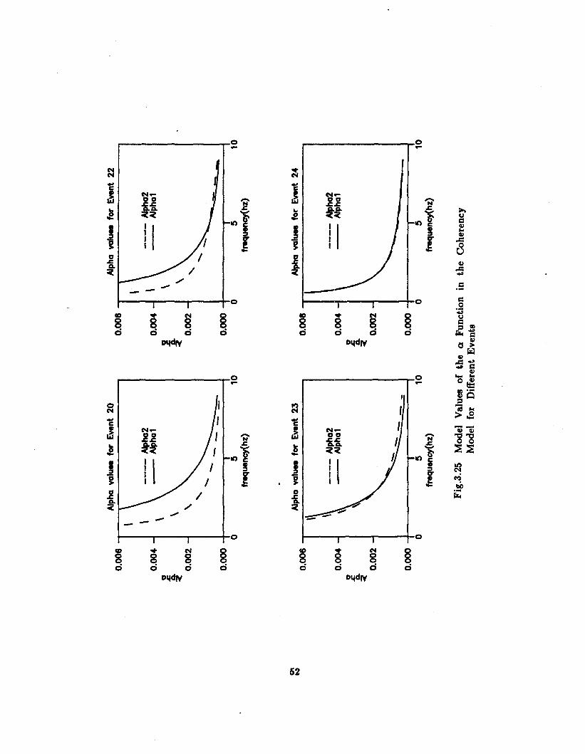
range, could be obtained for ad/) and a2 (J), if more raw data were available. Figures 3.22
through 3.24 show the model errors in loss of coherency for Event 45 calculated for all the
available distances. The model al (J) and a2 (I) functions for all 17 events were determined.
The results for Events 20, 22, 23, 24, 41, 45, 46, 47 are shown in Figs. 3.25 and 3.26.
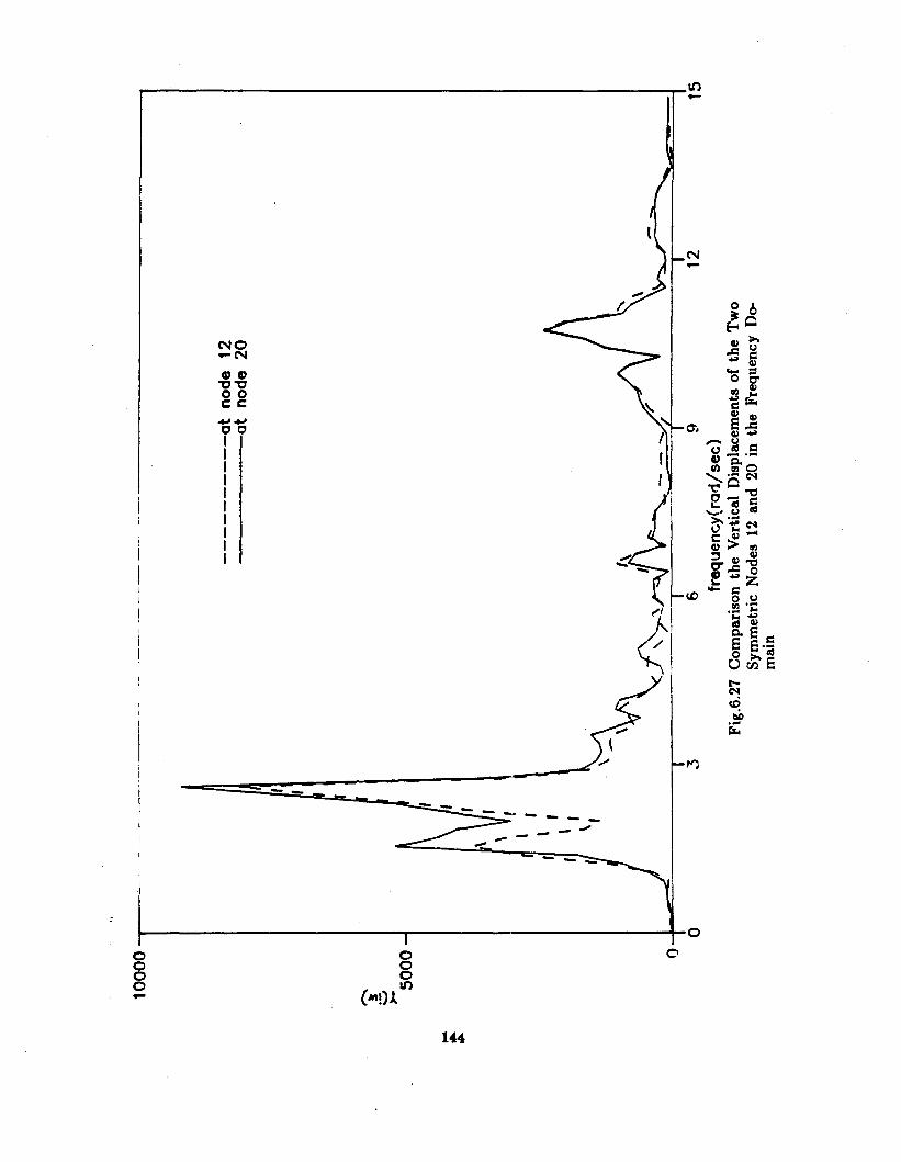
From Table 3.6, and the calculated loss of coherency values, it is observed that the {3
values are dependent on peak ground accelera~ion. Figures 3.27 and 3.28 show the {3I and {32
relations, respectively, with respect to PGA. The {3 values are seen to decrease with increasing
PGA which corresponds to an increase in loss of coherency values. This is because the ground
motion energy dissipation from wave propagation through the same distance, is the same. A
ground motion having a higher PGA usually contains a higher amount of energy. Consider
two waves travelling along the same path between points P and Q, with energy content E I
and E2 at the point P. If 8 is the amount of energy dissipated by the waves between P
and Q, then the proportional energy dissipation is defined to be ;1 and ;2' respectively.
If E I > E2 , then 8/EI < 8/E2
That is, the proportional energy dissipation of a ground motion with a higher PGA is smaller
20
than the proportional energy dissipation of a ground motion with a lower PGA, along the
same path. It follows that the ground motion, that has the higher proportional energy
dissipation, has smaller ·loss of coherency values along the same path. Another property that
can be noticed is that (31 is larger than (32 for the events with azimuths between 900 and
1800 , except for Event 33, and (31 is smaller than (32 for the events with azimuths in the
range 00 - 900 and 1800- 2700
• This phenomenon takes place because of the presence of
a mountain to the north-west of the SMART-1 site while the terrain is flat in all other
directions. This mountain will certainly disturb the propagation of plane waves.
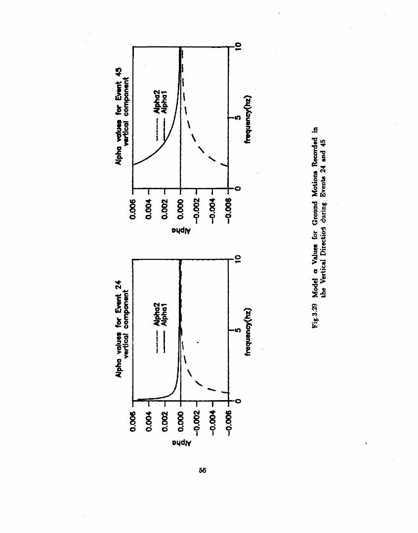
The same methods of processing were used for the ground motions recorded III the
vertical component of Events 24 and 45. The (3 values obtained were (31 = 1.795 X 10⁻³ and
(32 = 1.442 X 10- 3 for Event 24, and (31 = 2.014 X 10- 4 and (32 = 1.066 X 10- 4 for Event 45.
The 6 constants in the a functions (a, b, c, d, e, and g) are 5.331 X 10- 4, -4.740 X 10⁻⁶
,
6.507 X 10- 5 , -3.891 X 10- 3 , -7.571 X 10- 5 and 1.025 X 10- 3 , respectively, for Event 24 and
1.455 X 10- 2, 1.711 X 10-\ -3.024 X 1O-S, -1.255 X 10- 2 , -1.255 X 10⁻⁴ and 2.327 X 10⁻³ ,
respectively, for Event 45. The a functions for the vertical components of the two events are
shown in Fig. 3.29.
21
Table 3.1 Velocity and Moduli Values
depthVp(mls) V (mls) v G(kg/cm2 ) E(kg/cm2 )(m) s
0-5 370 120 0.441 264 761
5-8 810 140 0.485 360 1069
8-13 1270 190 0.488 663 1973
13-31 1330 220 0.486 889 2642
31-34 1330 280 0.477 1440 4254
34-48 1250 250 0.479 1148 3396
48-60 1220 270 0.474 1339 3947
60-80 1470 320 0.475 1881 5549
80-150 1540 480 0.398 4232 11833
V =P wave velocityp
V =S wave velocitysp =Bulk density = 1.8gm/cc
v = Poisson ratio
22
G=Shear modulus=pV2
sE=Young's modulus=2G(1+v)
t.:I
W
Tab
le3.
2C
hara
cter
isti
csof
the
17R
ecor
ded
Eve
nts
Dep
thE
pic
en
tral
Azi
mut
hS
tati
on
sM
axim
umA
ccele
rati
on
s(g
all
ev
en
tM L
(km
)D
ista
nce
(Deg
)T
rig
gere
dV
EWN
S
20
6.4
87
819
63
63
1.8
62
.88
6.1
22
6.4
28
35
21
73
53
6.7
71
.16
1.0
23
6.6
37
85
12
82
31
2.4
26
.13
6.1
21
6.9
11
85
13
031
15
.45
1.1
61
.9
25
6.8
28
75
11
83
51
1.0
35
.63
8.5
29
6.0
93
56
93
02
3.5
83
.36
5.0
30
6.3
612
96
33
23
1.9
.6
6.2
78
.7
315
.91
18
79
37
36
.81
01
.06
9.2
33
6.5
31
51
04
36
38
.21
18
.69
7.2
36
6.3
61
711
03
65
5.4
11
3.1
82
.8
37
5.3
23
016
73
31
1.0
63
.07
3.4
40
6.5
16
67
19
53
77
2.5
21
0.5
25
1.1
116
.22
271
19
23
72
8.5
62
.59
9.8
15
7.0
71
91
75
36
11
0.3
17
8.0
25
1.0
16
79
175
17
79
17
5
18
79
17
5
~ til-
Tab
le3.
3P
aram
eter
sof
the
Pow
erS
pect
ral
Den
sity
Fun
ctio
ns
Ev
ent
24E
ven
t45
win
dow
NS
EWN
SEW
DN
num
ber
f gw
Sf g
wS
f gw
Sf g
wS
f gw
Sg
0g
0g
0g
0g
0
1.3
01
.98
.Ox1
04.9
51
.05
.33
2.0
3.O
x105
.84
1.7
5.O
xl05
.80
4.5
2x10
52
.3x
lO
2.2
61
.04
.Ox1
05.3
01
.21.
Ox1
06.8
3.9
07
.80
1.2
7.8
04
.58x
105
1.2
xl0
1.2
xlO
3.5
8.8
05
.71
1.0
5.6
0.5
06
.95
.50
6.4
1.6
03x
105
7.3
xlO
8.1
xl0
4.5
xlO
9.5
xlO
Table 3.4 Scale Factors for the Power Spectral Density Functions
Window Event 24 Event 45
number NS EW DN NS EW DN
1 1.0 1.0 1.0 1.0 1.0
2 1.34 0.94 1.49 1.24 1.0
3 1.65 1.06 2.07 1.80 2.82
Table 3.5 Parameters for the Shape Functions
Event 24 Event 45
NS EW DN NS EW DN
t ma% (8) 8 11 12 12 8
a 0.206 0.15 0.1347 0.1347 0.206
b 0.0078 0.00413 0.00347 0.00347 0.0078
25
~
Tab
le3.
6C
alc
ula
ted
fJV
alue
s
Ev
ent
20
22
23
242
529
fJ 15
.35O
xl0-
41.
l3O
xl0
-45
.29O
xl0-
42
.622
x1O
-42
.39O
xlO
-43
.55
Ox
l0-4
3.6
7Oxl
0-4
3.1
1O
xl0-
41.
86O
x1O
-4-4
1.82
Oxl
0-4
6.3
1Oxl
O-4
fJ 21
.21
1x
l0
Ev
ent
3031
333
637
40
fJ 12
.25O
xl0-
44
.62O
xl0-
42
.81O
xl0-
43.
53O
xlO
-47
.91
Ox
l0-4
-59
.323
xlO
5.1
00
xlO
-44
.82O
xl0-
43.
71O
xlO
-42
.83O
xlO
-46
.83O
xlO
-4-4
fJ 21.
421x
lO
Ev
ent
4145
4647
48
fJ 13
.06
2x
l0-4
1.10
9x1O
-4-3
7.4
2Oxl
0-4
-31.
193x
l01.
391x
lOfJ 2
6.8
94
xl0
-46
.73O
xlO
-59.
01O
xlO
-4-3
-41.
202x
lO4
.723
xlO
N ~
Tab
le3.
7C
onst
ants
inth
eQ
Fun
ctio
ns
Ev
ent
ab
cd
eg
20
-28
.59
Ox
lO-5
-34
.55
4x
1O
-3-5
-4.3
39
x1
O-4
1.3
56
xlO
-1.9
33
xlO
1.6
97
xlO
22
8.6
39
x1
O-3
6.2
19
xlO
-5-3
2.6
44
x1
O-3
-5.2
64
xlO
-5-4
-1.2
51
xlO
5.2
61
xlO
23
-3-5
-3-3
2.4
20
x10
-5-6
.4M
9x1O
-49
.00
3x
lO7
.24
3x
lO-1
.44
5x
lO7
.01
6x
lO
24
-3-6
2.0
42
xlO
-5-3
2.5
90
x10
-6-1
.05
Ox
lO-4
3.1
13
xlO
-6.6
35
xlO
3.2
86
xlO
25
-32
.64
Ox
lO-5
-6.7
49
xlO
-4-2
-4-3
7.0
16
xlO
1.5
83
xlO
1.9
03
xlO
-3.5
28
xlO
29
-4-5
-3-3
-4-3
-4.1
77
xlO
-9.9
38
xlO
1.2
23
xlO
8.7
67
xlO
1.2
03
xlO
-2.0
07
xlO
30
-2-5
-4-3..
-5-1
.11
8x
1O
-3l.
06
6x
lO2
.65
1x
lO-9
.98
8x
lO6
.65
5x
lO5
.88
3x
lO
31-3
7.6
6O
xlO
-5-3
-3-5
-1.
168
xl0
-37
.48
3x
lO-1
.37
5x
lO7
.06
2x
lO5
.55
3x
lO
33
3.6
24
x1
O-3
-5-5
'-3
-5-3
-1.7
05
xlO
3.6
78
xlO
5.8
15
xlO
5.6
87
xlO
-l.O
O5
xlO
36
8.2
4O
xlO
-4-5
-4-3
-5-4
1.2
67
xlO
-1.4
76
xlO
7.4
68
xlO
1.9
43
xlO
-6.9
11
xlO
37
-2-4
-3-1
.12
4x
10
-2-4
-31
.18
6x
lO1
.45
1x
lO-2
.49
8x
lO-l
.96
6x
lO3
.29
7x
lO
40
-29
.33
Ox
lO-5
-38
.09
0x
1O
-3-5
-31
.03
7x
lO-1
.82
1x
lO4
.08
3x
lO-1
.OO
7x
lO
411
.27
9x
1O
-3-6
-4-3
4.2
82
xlO
-5-4
-9.6
56
xlO
1.2
25
xlO
4.3
55
xlO
-7.4
03
xlO
45
-3-5
-4-3
-7.5
83
xlO
-6-4
3.8
53
xlO
-1.8
11
xlO
1.1
77
xlO
5.1
63
xlO
-l.9
05
xlO
46
-31
.80
2x
10-5
-41
.11
Ox1
0-3
-55
.65
9x
1O
-42
.02
5x
lO-2
.66
8x
lO-4
.70
1x
lO
47
-3-6
-4-3
-1.0
2O
xlO
-5-4
1.8
83
xlO
5.1
72
xlO
-1.3
95
xlO
-1.8
72
xlO
3.0
05
xlO
48
5.2
1O
xlO
-3-5
-3-2
.33
9x
1O
-4-5
-46
.38
3x
lO-1
.03
6x
lO-6
.47
3x
lO9
.68
7x
lO
o•
CD 4-------.1.------+(\J
123.0
0.0 so.o tOtI.....__-I'
~s
122.0LLJNGITUDE
•en -4--...1-------,.------+N
121.0
o•
lJ)(\J
o
wo:::>f-.......f-a:-10
•::::r(\J
Fig.3.1 Map of the SMART-l Location
28
...Hl..
.... ..HI ..... ..
....1-01.. .. .... .. .... ..A.A· .... ....
.. ....
....
..E-01
..E-D2
o. 1.Ir:•
2.
Fig.3.2 The Configuration of the SMART-l Array
29
Su
bsu
rfac
eg
eolo
gy
alo
ng
pro
file
A-C
'
TC
-PTe
-oT
&-5
40
......".:::.
7..;:c:-:>.·...
.....~;;>:;~=:-:.
----
----
--.....
..,'
~"/
//
'M
ioce
ne
Arg
illi
jtE
oce
ne
Sla
teS
late
I.(3
30
0m
/sec
)17
~
Rec
ent
All
uv
ium
(SO
O-l
OO
Om
/sec
)O
lig
oce
ne
toM
ioce
ne
Arg
illi
te,S
an
dst
on
e
scale
II
II
•
o2
km
Oli
go
cen
eto
Mio
cen
eA
rgil
lite
,S
and
sto
ne
~~
Eo
cen
eto
Oli
go
cen
eS
and
sto
ne
Eoc
ene
Sla
te(3
30
0)
Eoc
ene
toO
lig
oce
ne
San
dst
on
eR
ecen
tA
llu
viu
m(5
00
-10
00
m/s
ec)
..........
_..
..••••
u••••••••
::;;
:;.....
••••••
,••~
•.........................
scale
JI
II
~km
Su
bsu
rfac
eg
eolo
gy
alo
ng
pro
file
D-D
'
Mio
cen
eA
rgil
lite
,(3
300
m/s
ec)
TO
-'"
!
Fig
.3.3
Tw
oN
orth
-Sou
thC
ross
Sect
ions
ofth
eS
MA
RT
-lA
rray
oU')·~~--_J...-__-.l_---"-----"r
'10. 0KM
.0. 0
o(I')·~
o11')·N+------r------..--------r----~
119.50 120.37 121.23 122.10 122.97Ll'NGlTUOE
0t-·::I'N
•20
0en,,24·ro • •25 23
~~-""05-·ro
-'Fig.3.4 Epicentral Positions of the 17 Recorded Events
31
d:m-lll--------.~iJ""llIIl'AaJl\.1
v•.
-.V
•.•
.-5
0.0
SEC
I,
,,
,,
,,
,,
I,
,,
,,
,,
,,
I,
,,
,,
,,
,,
I•
•t
,,
,,
,,
I
o10
2030
40
50.0
gal
Id:
o-O
SI -5
0.0
50.0
gal
Id:
m-O
SI -5
0.0
50.0
gal
Id:
i-O
SI -5
0.0
50.0
gal
IC
lId:
o-O
O..,
-50
.050
.0g
alI
d:i-
llI -5
0.0
50.0
gal
Fig
.3.S
Rec
orde
dA
ccel
erog
ram
sin
NS
Dir
ecti
ondu
ring
Eve
nt24
c. '"
40
00
00
30
00
00
.........~200000
o tn
10
00
00
4.0
06
.00
freq
uenc
y(hz
)8
.00
10
.00
Fig
.3.6
Ave
rage
dPo
wer
Spe
ctra
lD
ensi
tyF
unct
ion
for
Ac
cele
rati
ons
Rec
orde
din
EW
Dir
ecti
ondu
ring
Eve
nt24
(Tim
eW
indo
w5-
10se
c)
:
,,-... - ---o rn
6000
000
4000
000
2000
000
10.0
08.
004
.00
6.0
0fr
f!q
ue
ncy
(hz)
2.00
o-=)iiiIiiiii
I..
...
I;-;
=;-y=
;II
».7
i,
j;
,,
j,iii'iii'iiiiii
ij
j•
0.00
Fig:
~.1
Ave
rage
dPo
wer
Spe
ctra
lD
ensi
tyF
unct
ion
for
Ac
cele
rati
ons
Rec
orde
din
EW
Dir
ecti
ondu
ring
Eve
nt24
(Tim
eW
indo
w9-
19se
c)
4.00
6.00
freq
uenc
y(hz
)2
.00
04.i
iiiii'iii
IIii
I;:
,I
II
1I
IIiiiiiiiiIiiiii
Iiiiiiiii
iI
0.00
50
00
00
1500
000
10
00
00
0
........ '--" o C/l
ColI
C1I
Fig
.8.8
Ave
rage
dP
ower
Spe
ctra
lD
ensi
tyF
unct
ion
for
Ac
cele
rati
ons
Rec
orde
din
EW
Dir
ecti
ondu
ring
Eve
nt24
(Tim
eW
indo
w18
-28s
ec)
25.0
020
.00
10.0
015
.00
freq
uenc
y(hz
)
8]0
II
II
I,r
f1
'1,
;iF
n,iiiiiiiii
iI
Ii
IIIiiiiiiiiiiiiii'
5000
00
1500
000
2000
000
81
00
00
00
o (f)
~
Fig:
:l.g
Ave
rage
dPo
wer
Spe
ctra
lD
ensi
tyF
unct
ion
for
Ac
eele
n.ti
ons
Rec
orde
din
EW
Dir
ecti
ondu
ring
Eve
nt45
(Tim
eW
indo
w5-
10se
c)
Cot~
1200
0000
0
8000
0000
--~ ....... tff
4000
0000
10.0
0'1
5.0
0fr
equ
ency
(hz)
Fig
.3.1
0A
vera
ged
Pow
erS
pect
ral
Den
sity
Fun
ctio
nfo
rAc~
cele
rati
ons
Rec
orde
din
EW
Dir
ecti
ondu
ring
Eve
nt45
(Tim
eW
indo
w9-
29se
c)
25.0
0
2000
0000
ell
OIl
1500
0000
~10
0000
00....
..- tff
5000
000 g~o',
~'n
,'5.60
II
I,
,,1o
.bb',
iI
Ii
1s.bb
ii
,i
,i
!..!.
'-'-.iiiIii
!..!.
I
freq
uenc
y(hz
)
Fig
.3.1
1A
vera
ged
Pow
erS
pect
ral
Den
sity
Fun
ctio
nfo
rA
cce
lera
tion
sR
ecor
ded
inE
WD
irec
tion
duri
ngE
vent
45(T
ime
Win
dow
28-3
8sec
)
4.0
06
.00
freq
uenc
y(hz
)2
.00
0i
IIIiiiiiiiiiiiiii
Iiiiiiiiii
IIIiiiiiIii
IIiiiii
II
II
I0
.00
10
00
0
3000
0
4000
0
""'
~20000
o Ul
~
Fig
.3.1
2A
vera
ged
Pow
erS
pect
ral
Den
sity
Fun
ctio
nfo
rA
cce
lera
tion
sR
ecor
ded
inV
erti
cal
Dir
ecti
ondu
ring
Eve
nt24
(Tim
eW
indo
w5-
10se
c)
40
.00
30
.00
0.0
01
1,"""-
Ii
II
ir-T
1--rTiii
,i
IIii'
,i
,i
II
IIii
iT
Il
.,--
,
0.0
05
.00
10
.00
15
.00
20
.00
tim
e(se
c)
10
.00
Q)
0-
o2
0.0
0..c (J
)
~
Fig
.3.1
3A
vera
ged
Env
elop
eF
unct
ion
for
Gro
und
Mot
ions
Rec
orde
din
EW
Dir
ecti
ondu
ring
Eve
nt24
.... ...
Q)
0.. o .c U1
15
0.0
0
10
0.0
0
50
.00
0.0
0 0.0
0
Fig.
3.14
Ave
rage
dE
nvel
ope
Fun
ctio
nfo
rG
roun
dM
otio
nsR
ecor
ded
inE
WD
irec
tion
duri
ngE
vent
45
8.0
0
Iii
Ii
1..-.-.....
11
1-,-
,-1
II
1I
11
1"
1I
1.,
....
,.·.
.,--,.
.,,·
,-r·-
"-T
1
5.0
010
.00
15
.00
20
.00
tim
e(se
c)
0.0
0 0.0
0
2.0
0
6.0
0
Q) C 04
.00
.c (f)
• N
Fig
.3.1
5A
vera
ged
Env
elop
eF
unct
ion
for
Gro
und
Mot
ions
Rec
orde
din
Ver
tica
lD
irec
tion
duri
ngE
vent
24
tim
ew
Indo
w(b
ee-S
.ee)
time
wIn
dow
(Jae
c-8
aec)
1414
1212
1010
Q.
8Q
.8
~0
S>
6
4
:i.--
-*~
•2 0
00.
02.
04.
00.
02.
04.
0fr
eque
ncy(
hz)
freq
uenc
y(hz
)
.• w
time
wIn
dow
(15
.ee-
2S
.ee)
tim
ew
Indo
w(2
0.e
e-JO
aee)
1414
1212
1010
Q.
8Q
.8
~6
~6
44
22
00
0.0
2.0
4.0
0.0
2.0
4.0
freq
uenc
y(hz
)fr
eque
ncy(
hz)
Fig
.3.1
6E
xam
ple
App
aren
tV
eloc
itie
sC
alcu
late
dby
F-K
Met
hod
for
Eve
nt45
ij5N
15-2
5SE
Cl.
ij6
HZRZ
IMUT
HOF
PERK
=lij
6RP
PARE
NTVE
LOCI
TY(k
m/e
8cJ
=5
.5MA
XIMU
MPO
WER
(cm
/e8c
)••2
=25
35
ij5N
15-2
5SE
C1.
95HZ
AZIM
UTH
OFPE
AK=
180
APPA
RENT
VELO
CITY
(km/e~c)
=6.
7MA
XIMU
MPO
WER
(cm
/••c
)••2
=21
67
-1.0
QII"
""
"'II"
"'IIIIIIIIIIIIII"
"'"
-1.0
-0.5
0.0
0.5
1.0
SLOW
NESS
(SEC
IKHJ
1.0
Oh
ilil..
..N
••iiiii.ii.,.;
••iiiiiiiii
iiii
(f)
O.O
F(
(J')
,...
UJ
•z :r ~
-0.5
(f)i: ~
0.5
u UJ
(J') -
-1.0
01
11
11
11
11
11
11
11
11
11
11
11
11
11
11
11
11
11
11
0
-1.0
-0.5
O.0
O.5
1.0
SLOW
NESS
(SEC
/KM
l
1•0
'iiiiiiiiiiiiiiii'
ii.
.,iiiiiiiiiiiiiiiiii
iJ
(J')
o.0
I="F_:!loJ>,'L-~
..,~
j
z :x ~-0
.5eni: ~
0.5
u w (J') -
:t
Fig
.3.1
7E
xam
ple
F-K
Dia
gram
for
Acc
eler
atio
nsR
ecor
ded
duri
ngE
vent
45
Loa. of coherency vatu.. of event 24NS component (x-50m,y-SOm)
1'0~~~
fO.~
0.0 -+----------~--------_4o 5
fNquency(hz)10
Lou of coherency va/u.. of event 24NS component (x-JOOm,y-300m)
1.0 -----------.;--.;--~-------~
0.0 +-----------,r-------------to 5
frequency(hz)10
Lo•• of coherency value. of event 24NS component (x-1SOm,y-1S0m)
1.0 ...,...---------.,;.,.----.,;.,.--~-----..,
0.0 +----------..,....-----------;o 5
frequency(hz)10
Fig.3.18 Comparison the Model Coherency Values with theRaw Data for Event 24
45
Loa. of coherency value. of ~nt 31NS component (x-50m,y-5Om)
1.0 .......-----------.;..---.:...--:....------.,
0.0 -+----------""T""---------'"'1o 5
hquency(hz)10
Lon of coherency valu•• of event 31NS component (x-50m,y-150m)
1.0 .......--------=---~-......;...-----_,
0.0 4----------~--------_;o 5
hquency(hz)10
Lon of coherency values of ~t 31NS component (x-50m,y-300m)
1.0 .......-------.:...-----:.--~----___,
~
10.5g
0.0 -1----------......---------""1o 5
hquency(hz)10
Fig.3.19 Comparison the Model Coherency Values with theRaw Data for Event 31
LG.. of coherency value. of event 45NS component (x-150m,y-50m)
1.0 -.::=~---::----..:-_-~_---.::;..--.-~--...,
0.0 -+----------...,..----------fo 5
hquency(hz)10
Lou of coherency value. of event 45NS component (x-15Om,y-150m)
Using Eqs.(4.5), (4.11), and (4.12), a set of spatially correlated time-histories Xi(t) (i =
1,2, ... ,n) can be simulated, and the corresponding ground motions ai(t) (i = 1,2, ... ,n)can be obtained by multiplying each time-history by a proper shape function ~(t). By this
procedure, one first simulates a time-history of motion for support point 1, and then, simu
lates a time-history for support point 2 by summing up wave contributions that are properly
correlated with the simulated motion for point 1. Similarly, the simulated time-history for
the motions of support point 3 will be correlated with those previously simulated for points
1 and 2, etc.. The first time-history of motion can be either a synthetic motion or a real
motion provided that it is compatible with the prescribed spectral density matrix S(w).
Instead of using Eq.(4.5) to simulate Xi(t), it also can be simulated more easily in the
frequency domain. To proceed with this new approach, express the Fourier transform of Xi(t)in the form
i
Xi(iwk) = I: Bim(Wk)[COSQim(Wk) +isinQim(Wk)]m=l
k = 1,2, ... ,N (4.13)
where Bim (Wk) is the amplitude at frequency Wk, and Qim (Wk) is the corresponding phase
angle which is to be determined. By transforming Eq.(4.5) into the frequency domain, it can
be shown that1
Bim(Wk) = 2~m(Wk)
Qim (Wk) = f3im (Wk) + <Pmk
(4.14)
(4.15)
Then, by using Eqs.(4.13)' (4.14), and (4.15), the Fourier transform Xi(iwk) of Xi(t) can be
determined. The time-history Xi(t) is then obtained by transforming Xi(iwk) back to the
The simulation method presented above is based on stationarity assumptions of the
ground motions even though the ground motions are actually nonstationary in both the time
60
and frequency domains. The ground motion nonstationary property in the frequency domain
can be simulated by the quasi-stationary method. This method is based on a quasi-stationary
assumption for the ground motion P-waves, S-waves and surface waves, as discussed in the
previous chapter. The total ground motion time-history is divided into three time windows
for different types of waves and the time-history in each window is assumed stationary and
simulated independently. The total ground motion time-history is obtained by combining the
time-histories in the three windows.
Combined with the method discussed above to simulate quasi-stationary ground mo
tions, the simulation method for stationary ground motions is still applicable. The only new
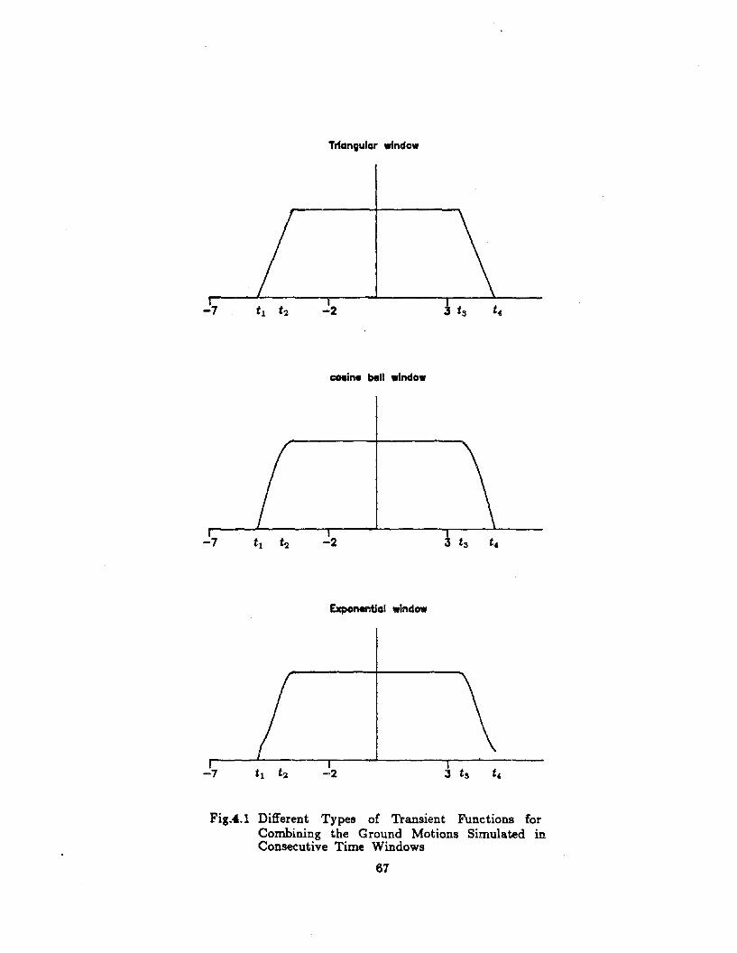
feature that needs to be studied is the combination. To combine the time-histories simulated
by different power spectral density functions in the different time windows, certain overlapping
of the different types of motion is needed; The transient part of the overlapping should be
made as smooth as possible in order to reduce the false energy and overshooting that will
be introduced by time-window cutting. The sum of the transient functions in the overlapping
part should be equal to one in order to keep the proper ground motion intensity in that
part. Several types of windows with different transient functions were tried for this purpose;
e.g., the triangular, cosine bell, and exponential types shown in Fig. 4.1. It was found that,
among the types tried, the exponential type produced the best results. As shown in Fig. 4.1,
with the four times t 1 , t 2 , ts , and t4 specified, the exponential window transient part used
is 1 - e- (t-td2
on the left side and e- (t-t 3 )2 on the right side.
4.5 Simulated Ground Motion Correction
Because of uncertainties regarding the initial conditions for the ground motion and the
position of the zero acceleration axis in the recorded accelerogram, predictions of the corre
sponding velocity and displacement time-histories are unreliable unless realistic adjustments
are made to account for these effects through baseline corrections to the accelerograms. The
adjustments can be made in either the time domain or the frequency domain. Many criteria
have been used to control the adjustments. The most common of these are: (1) zero mean
acceleration, which implies the initial and ending velocity values are the same, (2) zero initial
velocity, (3) zero initial displacement, (4) minimum mean square velocity , which implies
minimizing the ground motion energy content, and (5) zero mean velocity which implies no
permanent ground motion displacement.
Berg and Housner (1961) suggested the following method, based on the above criteria,
for adjustments in the time domain. The acceleration null line is assumed to have the shape
of a parabola which is determined by the method of least squares. The constants of the
parabolic equation should minimize the computed mean square of the velocity. After this
correction, both the acceleration and velocity terminate at the end of the motion. Using
61
the same criteria and the same second order parabolic null line assumption for acceleration,
Kausel and Ushijima (1979) suggested a method of making adjustments in the frequency
domain.
Another correction for the simulated ground motions is their response spectrum. Once
a response spectrum has been specified for a given site, ground motion time-histories can
be adjusted to be compatible with the specified spectrum. A method by Scanlan and Sachs
(1974), that can be used for this purpose, is based on the fact that the Fourier spectrum
of the ground acceleration time-history is equal to the velocity response spectrum for zero
damping. The procedure is (1) to calculate the velocity response spectrum fill' (2) to cal
culate the ratio of fill to the specified response spectrum S'n a = ~, (3) to multiply the
Fourier series of the time-history by a, and (4) to inverse FFT the result back to the time
domain. The velocity response spectrum for this corrected motion can be evaluated and the
above procedure repeated. Through this iterative procedure, an accelerogram compatible with
the spectrum is obtained. Usually, only 3 iterations are needed to make fill converge to a
satisfactory result.
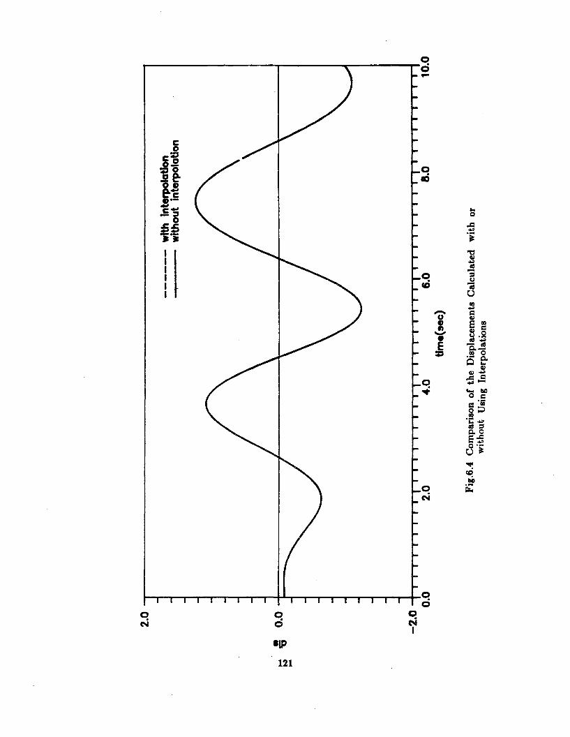
4.6 Ground Motion Time-History Interpolation
When multiple inputs are specified for large structures, spatially correlated ground
motion time-histories at all structure-foundation contact points are needed. If the number
of contact points is large, the simulation of these motions becomes expensive. Therefore,
an interpolation method is suggested here to reduce costs. By this method, ground motion
time-histories are simulated at a limited number of support points, and at all other points,
the ground motion time-histories are interpolated in the frequency domain by adjusting phase
angles and amplitudes to provide the proper cross correlations and power spectral contents.
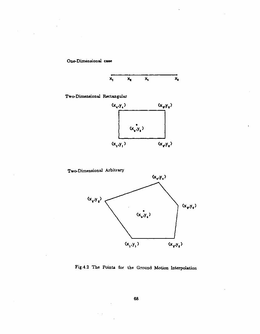
The interpolation function used is derived using the shape function idea. Consider the
one-dimensional case shown in Fig. 4.2, where Xl, Xz and Xs are the points where the ground
motion time-histories are to be simulated, and Xk is an arbitrary point where the ground
motion time-history is to be interpolated. The interpolation function for the one-dimensional
case ISnn (Xk - Xi)
I:::: 1i¢i
fik = --=-:----,-n (Xi - xdi= 1i¢i
j = 1,2, ... ,m (4.16)
where m is the total number of points at which the ground motion time-histories are sim
ulated, n is the total number of structure-foundation contact points, Xi, Xi and Xk are the
corresponding coordinates, fik is the interpolation function representing the contribution to
the ground motion at point k from the ground motion at point j. For the two-dimensional
62
case, see Fig. 4.2, the interpolation function is
nn [Yk - Ik(i, i + I)Ji=li .. i
lik = --.:....:n'---------
n [Yi - h(i,i + 1)]i=1i .. i
i= 1,2, ... ,m (4.17)
where Y" Yk are the corresponding coordinates, and 110 (i, i + 1) IS the value on the line
connecting points i and i + 1 at Xk; in general;
~( .. 1) Yi+l-Yi( )Jk I, 1+ = Xk - Xi + YiXi+l - Xi
(4.18)
If Xi = Xi+l or Yi = Yi+l, Eq.(4.18) becomes h(i,i + 1) = Xi or h(i,i + 1) = Yi, respectively.
Using the above interpolation functions, the ground motion time-history at any support
point can be interpolated using the time-histories simulated at the control points. The ground
motion time-history at point k is interpolated in the frequency domain using
(4.19)
where Ak(iw) is the Fourier transform of ak(t) at frequency Wj Ai(iw) is the amplitude of
the time-history ai(t) at point j at frequency Wj 4>i is the phase angle of ai(t) at Wj d;'k is
the projected distance between points j and k in the wave propagation direction, and v(w)is the apparent velocity at W. It can be shown that the interpolated time-history ak (t) will
have the correct phase differences and cross correlations.
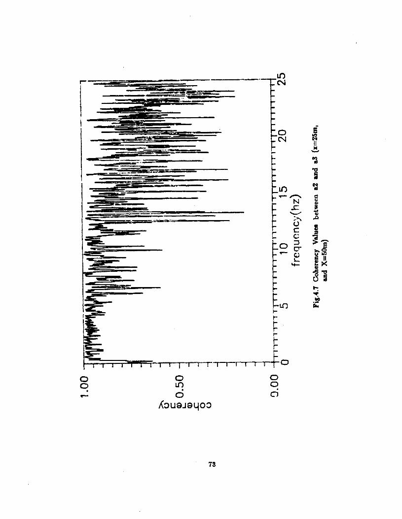
An example interpolation for the one-dimensional case was calculated using three sta
tions located 25m apart in the direction of wave propagation. The ground motion time
histories at the two end points, am and 50m, were simulated by using the coherency model,
Eq.(3.9), three segments of quasi-stationary motion having power spectral densities of the
Tajimi-Kanai type. All coherency and power spectral density function parameters were based
on those obtained for the NS components recorded during Event 45j see chapter 3. The
apparent velocity was arbitrarily assigned the low value of 35m/sec in order to see the cross
correlation values more clearly. Figure 4.3 shows the simulated acceleration time-histories after
iteration to be compatible with the Newmark and Hall (1969) response spectrum normalized
to 0.3g PGA, where al and a2 are simulated at am and 50m, respectively, and a3 is inter
polated at 25m. Figures 4.4 and 4.5 show the cross correlations of the three time-histories
before and after the response spectrum compatible iterations. It is obvious that the cross
correlation values are compatible with the prescribed wave propagation property. Also it can
be seen that the cross correlation values remain almost the same, and the phase difference
63
exactly the same before and after the iterations. This is because the iteration procedure only
works on the Fourier amplitudes, not on the phase angles. Figures 4.6 through 4.8 show
the loss of coherency values between the three time histories. Figures 4.9 and 4.10 show the
power spectral density functions of the three time histories. From these results, it can be
seen that the interpolated time-history satisfies the prescribed cross correlation structure and
the power spectral density function.
4.7 Examples
Using the method discussed above and the coherency model presented in the previous
chapter, realistic examples of spatially correlated ground motion time-histories were simulated
giving the following results:
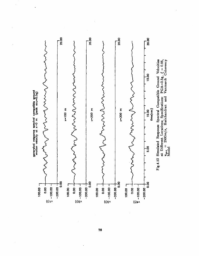
Spatially correlated stationary ground motion time-histories were simulated at four
stations along an epicentral direction separated 100m from one another (x=O; 100; 200;
300m). These time-histories with 20sec duration and ~t = 0.02sec were simulated using the
following specifications:
(a) The stationarity assumption was used with the Tajimi-Kanai (1960) power
spectral density function, Eq.(3.1) having parameters €g = 0.6 and wg =
51rrad/sec, and with So = 1.0.
(b) The Harichandran and Vanmarcke (1984) coherency model was used with
parameters A = 0.736, a = 0.147, and a spatial scale of fluctuation (J(w) =3300[1 + (1.~1r )2]-,1. The apparent wave velocity used was 1) = 2.5km/sec.
(c) The shape function, Eq.(3.5), suggested by Amin and Ang (1968) was used
with t 1 = 2sec, t 2 = lOsec and 10 = 1.0.
(d) The baseline correction was carried out by first filtering out the energy for
f ::; 0.5hz, and then using the time domain baseline correction method.
(e) The Newmark and Hall (1969) 5% damped design response spectrum, nor
malized to a 0.5g PGA, was used.
The four simulated ground motion time-histories are shown in Figs. 4.11 through 4.13,
expressed in terms of acceleration, velocity, and displacement, respectively. Figures 4.14 and
4.15 show the auto and cross correlation coefficients of the four time-histories, respectively.
From the cross correlation coefficients, it can be noticed that the proper phase differences
occur between the four simulated time-histories. Figure 4.16 shows comparisons between the
power spectral density functions of the simulated ground motions before the iterations to
be compatible with the response spectrum and the prescribed Tajimi-Kanai power spectral
density function. It can be seen that they match well, except for the apparent discrepancy
64
of high values in the low frequency portion of the spectrum at x = 300m, which can be
attributed to the random nature of the process. Figure 4.17 compares the loss of coherency
values with the prescribed model. It can be seen that at ~x = 300m, as the frequency
increases, the compatibility is not very good. This is because the calculated loss of coherency
values were not smoothed, and as the distance increases, the coherency values will be lower,
so that the noise will tend to be more dominant in the calculated values since the noise
level is increasing with frequency; the level is 0.35 at 1Hz and 0.45 at 10HZj see chapter
3. Figure 4.18 shows the calculated response spectra after two iterations compared with the
prescribed Newmark and Hall design response spectrum.
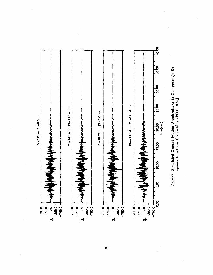
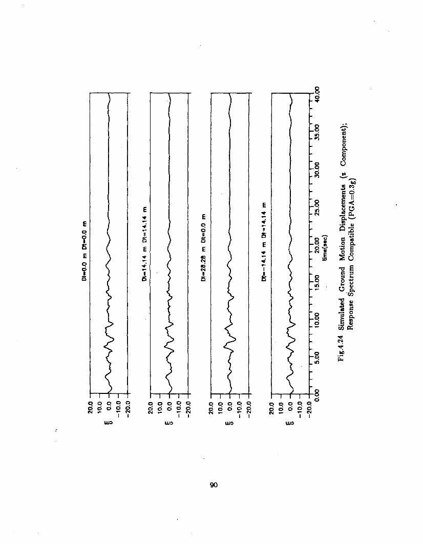
Another example considered was the simulation of spatially correlated ground motions
at each corner of a 20m rectangular foundation. The ground motions were simulated for the
x, y and Z directions. Suppose a wave propagates in a 450 direction to the foundation. Then,
in terms of the distances d~j and ~j as defined before, the coordinates of the corner points
are (0,0), (14.14,14.14), (28.28,0), and (14.14, -14.14), respectively. The ground motions were
first simulated in the wave propagating direction, transverse to the wave propagating direction,
and the vertical direction, independently. Because the wave propagating direction generally
coincides with the principal direction, the ground motions in that direction are uncorrelated
with the ground motions in its transverse direction, likewise, the vertical component of ground
motion is independent of the ground motions in the horizontal directions. The ground motions
in the x and y components were obtained by rotating the horizontal ground motions to these
directions. The simulated ground motions satisfy the following specifications:
(a) A quasi-stationarity assumption was used for all three components. The
time window width and the parameters used for the Tajimi-Kanai power
spectral density functions were those obtained by processing SMART-1 data
for Event 45; see Tables 3.3 and 3.4. The power spectral density functions
were all normalized using So = 1.0. The corresponding scaling factors in
Table 3.4 were then applied.
(b) The suggested coherency model, Eq.(3.9), was used with the results obtained
for Event 45 as shown in Table 3.6 and Table 3.7.
(c) The same shape function, ·Eq.(3.4), with the results obtained for Event 45,
was used with the parameters in Table 3.5.
(d) The same baseline correction procedure was used as in the previous example.
The Newmark and Hall design response spectra with damping ratio 0.05
normalized to 0.5g PGA for horizontal components and 0.3g PGA for the
vertical component were used as the target response spectra.
65
Figures 4.19 through 4.21 show the simulated accelerations for x, y, and z components,
respectively. Figures 4.22 through 4.24 show the corresponding displacements. From these re
sults, it can be noticed that the cross correlations of the components were well controlled.
The two horizontal components are independent of the vertical component which has the
highest frequency content and lowest intensity. These results all coincide with the observed
ground motion records. Figures 4.25 through 4.27 show the comparisons between the calcu
lated response spectra and the target response spectrum. Good results were obtained after
two iterations. It can be seen that the convergence is very good.
A final example was generated to illustrate the interpolation problem. Assume there
IS a 50m rectangular foundation. The ground motion time-histories were simulated at the
four corner points with coordinates (0,0), (50,0)' (50,50), (0,50). Five ground motion time
histories at (25,0), (50,25), (25,50), (0,25), and (25,25) were obtained by interpolation.
Suppose the wave comes in the x direction. The four simulated ground motions all satisfy
the specifications of Event 45 as given in the previous example for power spectral density
functions, coherency, and shape functions. The baseline correction procedure used was the
same as in the previous example. The Newmark and Hall design response spectrum for 5%
damping ratio normalized to the 0.3g PGA level was used again as the target spectrum.
Note that, in order to save computing time, the interpolation procedure should be carried
out after the iterations. Following this procedure, the response spectra can be interpolated
the same way as the time histories. If the response spectra are the same for all interpolated
time histories, the response spectrum of the interpolated time-history will still be compatible
with the target response spectrum since the interpolating procedure actually works on the
amplitudes and phase angles independently while the response spectrum is controlled by the
amplitudes. Figure 4.28 shows the accelerograms in the x direction before iterations. Figure
4.29 shows the accelerograms after 3 iterations. Figure 4.30 shows the displacements after
3 iterations. From these figures, it can be concluded that the ground motion properties are
properly controlled by the simulation and interpolation procedures.
66
Triangular window
coelM bell window
-2
Exponential window
-2
Fig.4.1 Different Types of Transient Functions forCombining the Ground Motions Simulated inConsecutive Time Windows
67
One-Dimensional case
Two-Dimensional Rectangular
(x.,y. )
Two-Dimensional Arbitrary
(x.,y.)
Fig.4.2 The Points for the Ground Motion Interpolation
68
30
40
30
40
20 20
10 10
30
0..
,--
I
200
100
na
...-.v
W'fl
l1II
o...
-10
0-2
00
-30
0I
iI
II
II
II
II
II
II
I1
,I
1I
II
II
II
II
II
II
II
II
II
1I
o
';j~g~l~I~.~JU.Jd'IIAIJ.L
~.1,.•1
.1
.."
'l-1
00
-20
0-3
00
II
,I
II
II
I,
II
II
II
I1
I1
-I
II
II
II
II
II
I,
II
II
II
I1
a3
00
i-
I
20
010
0
'0=~gg
I~'lll'~m'
'nmr~
'~II'If1'P"
''r.-~.
-I
-30
0r~
a10
20
30
40ti
me(
sec)
~
Fig
.4.3
Exa
mpl
eof
Sim
ulat
edG
roun
dM
otio
nA
ccel
er
atio
nsC
ompa
tibl
ew
ith
New
mar
kan
dH
all
De
sign
Res
pons
eS
pect
rum
of5%
Dam
ping
Nor
m
aliz
edto
0.3g
(al
and
a3ar
eS
imul
ated
,an
da2
isIn
terp
olat
ed)
.1an
das
':I 1 ~0
.50
1.00
iI
f) c o .- -+J o_
-0
00
l\.
....I,~
¥:J~
V,
4"
'-II
-'/
hA
l"f
N\'
An
'-~v
VF
\:&,
u.
...uc
Yt~
t.._
'(.,.~
,4
Q*(
VA
-'\.
t o o I " ~-0
.50
L o
~ o
10.0
08
.00
-1.0
0,iiiIi'
,,
1I
,,
,,
,,
,,
,I
,,
,,,.
.,..
.,1ii'
,I
,I
,I
iI
II
II
II
,I
Ii
II
II
I,
0.00
2.0
04.
006.
00ti
me(
sec)
Fig
....
Cr0
88C
orre
lati
onC
oeff
icie
nts
ofth
eS
imul
ated
and
Inte
rpol
ated
Gro
und
Acc
eler
atio
nsbe
fore
Iter
atio
ns
10
.00
---------------.-
I
-1.0
0t
II
IIii
Ii
II
I,
,I
,i
II
II
iI
II
I,
,I
II
',
,I
II
,I
IIIiiiiiiiiiiiiii
0.0
02
.00
4.0
06
.00
B.O
Oti
me(
sec)
1.00
3CJ
1~
1."
."."
0.5
0~~
~~
enCJ
';;c
Ja :;; 0
~
"0
.00
I-'
... ... a 0 I en rn a-0
.50
... 0
Fig.
of.S
Cro
ssC
orre
lati
onC
oeff
icie
nts
ofth
eS
imul
Med
and
Inte
rpol
ated
Gro
und
Acc
eler
atio
ll8
afte
rJ&
.er
atio
ns
201
01
5fr
equ
ency
(hz)
5
",L~
....1
IIl....
.It..
IiJII
II
I'
.,
dI
t_.I.
.\
o0
.00
1.00
~ o c ~0
.50
Q)
.c o o
... ..,
Fig
.4.6
Coh
eren
cyV
alue
sbe
twee
na1
and
a2(x
=O
m,
and
X=
25m
)
Lf)N-
0 EIn
N NII
..··=-:-mE ..>C
~.... -_. ~..--- .,_~___sa......,~ _.
"tl- ;sa.
T •~Lf)
~,........ s:lN ell
-. ; !.c'--" ell
1- ----. :~ .D
1*0 !
in r- r:: ~
% l- e;~-0 :::l
cr >.~~ C yin
'- i II"t- ~><
..c::"tl
~~8 ;....•..0....I1Iot
E~r
~o0 0 00 L(') 0. . .~ 0 a
AoueJe400
73
1.00
-,--------
~ o c ~0
.50
(l)
.c o o~ ...
0.0
0o
510
15
freq
uen
cy(h
z)2
025
FiS·
•.8
Coh
eren
cyV
alue
sbe
twee
nal
and
a3(x
=Om
,an
dX
=5O
m)
0.15
,,
0.15
II
"1
x-5
0m
0.10
0.05
i
8
x=O
m
35
hque
ncy(
hz)
or
y
~}J
H'T
'."'¥
'rf'l
.-..v~.
F¥i
0.0
0-=t
L,,
iIIii
ii5
81
00
.00
-l~
II
II
II
II
II
10
0.
3~
0.05
0.10
s ... en
~ C1l
FiS.
4.9
Pow
erS
pect
ral
Den
sity
Fonc
tioD
Bfo
ral.
and
a3
;:
0.1
5
0.1
0
s C'f '" 0
.05
0.0
0o
x=25
m
35
freq
uenc
y(hz
)10
Fig
.4.1
0Po
wer
Spe
ctra
lD
ensi
tyF
unct
ions
for
a2
gen
erat
edre
spo
nse
spec
tral
com
pat
ible
gro
un
dm
otio
nac
cele
rati
on
at
x=O
m~peak
acc=
O.5
g)
10
00
.00
50
0.0
0~
0.0
0--
t---
-\N
IU"W
'~
-50
0.0
0a
-10
00
.00
-15
00
.00
1I
0.0
02
0.0
0
x=
10
0m
20
.00
20
.00
x=
20
0m
x=
30
0m
10
00
.00
50
0.0
0S0.00~
~-5
00
.00
nNw.
~-1
00
0.0
0-1
5C':.
1J0
-t 0.0
;--0-~~===
1
10
00
.00
50
0.0
0-;:
;-0
.00~V\\.nNN.JIJI
'j;}
-50
0.0
0o
-10
00
.00
-15
00
.00
--1I
0.0
0
~ ~.
20
.00
~oo
lQO
Ol~OO
tim
e(se
c)
Fig
.4.l
lS
imul
ated
Res
pons
eS
pect
ral
Com
pati
ble
Gro
und
Acc
eler
-at
ions
atD
iffe
rent
Loc
atio
ns;
Spe
cifi
cati
ons:
PG
A=
0.5
g,
€=
0.05
,tJ
a{'
p=
25
00
m/s
,H
aric
hand
ran
and
Van
mar
ckC
ohe
renc
yM
odel
10
00
.00
50
0.0
0-;:
;-0
.00
II..ft
.Illla
..M."~
.••la
Il.ln
.al
_5
00
.0
0'Jl"r'W
\I"V
\f'
\PW
V'''
'''-''
\
-10
00
.00
-15
00
.001 1;
-111
,,--'-
1-.,.
.'~;I;
--r,--
rl-"r
--,---
:~:-=-
....,.
.--r-I
-..-r-
r-""
'-~-
--'-
--0
.00
IIi'
I,
I'I
II
i
100.
00
gene
rate
dre
spon
sesp
ectr
olco
mpa
tibl
egr
ound
mot
ion
velo
city
atx=
Om
(pea
ko
ee-0
.59
)
0.0
0-+
--.
3 -;-1
00
.00
20
.00
-20
0.0
0I
I0
.00
x-1
00
m
O.OO~
3 ~-1
00
.00
10
0.0
0
20
.00
x...2
00
m
-20
0.0
0I
I0
.00
04
OIl
10
0.0
0
O.OO~
-::;-
I-
,~
-10
0.0
0~
!---------------------------------;]1
-20
0.0
01-
20.0
00
.00
x-3
00
m
100.
00l
S0
.00j
-v
'VV
'~
t-1
00
.00
-20
0.0
0I
II
II
II
,I
Ii
II
I1
II
II
I0
.00
5.0
010
.00
15.0
02
0.0
0tl
me(
sec)
Fig
A.1
2S
imul
ated
Res
pons
eS
pect
ral
Com
pati
ble
Gro
und
Vel
ocit
ies
atD
iffe
rent
Loc
atio
ns;
Spe
cifi
ca.ti
ons:
PG
A=
0.5
g,e=
0.05
,va
l'''
=2
50
0m
/s,
Ha.
rich
andr
anan
dV
anm
arck
Coh
eren
cyM
odel
20
.00
gen
erat
edre
spo
nse
spec
tral
com
pati
ble
grou
ndm
otio
ndi
spla
cem
ent
atx.
.om
(pea
koc
c""O
.5g)
20.0
0
O.OO~
;;-2
0.0
0
-40
.00
II
0.0
0
..-.. .. '-"
xco1
00
m
s ~-2
0.0
0~IL
----
----
----
~,
-40
.00
20
.00
0.0
0x.
..20
0m
~
20
.00
O.OO~
..-.. .... '-" ~
-20
.00~L -
--------------------------------:JI
-40
.00
20.0
00
.00
x-J
OO
m
20
.00
,.....
0.0
0t
./
l'-2
0.0
0J
-40
.00~
II
II
IIiii
Iii
II
II
I,
II
0.0
05
.00
10.0
015
.00
20
.00
tlm
e(se
c)
Fig
.4.1
3S
imul
ated
Res
pons
eS
pect
ral
Com
pati
ble
Gro
und
Dis
plac
em
ents
atD
iffe
rent
Loc
atio
ns;
Spe
cifi
cati
ons:
PG
A=
0.5g
,e=
0.05
,va
l'''
=25
00m
/8,
Har
icha
ndra
nan
dV
anm
arck
Co
here
ncy
MO
del
1.00
II
auto
corr
elat
ion
func
tion
ofth
ege
nera
ted
grou
ndm
oUon
acce
lera
tion
s
1.00
II I
~
1.00
iI
0.5
0
N ~0
.00
0.5
0
1.00
II
-0.5
0-0
.5
°L
-1.0
0II
II
II
II
IIII
IrIT
TT
rtT
TT
"I
II
II
I-1
.00
II
II
IIT
TT
TT
Tl"
-I""
~0
.00
2.00
4.00
6.00
0.0
02.
004.
006
.00
tlm
e(se
c)tl
m.(
••c)
~O.OO~
~
0.0
0
0.5
00
.50
I.'l
:.
~~]
,~~i
i
-1.0
0'I
II
II
II••,.
IIrT
TT
IIII
•rr
~-1
.00-f"
rr,I
II
I,
II
I,
IrInTT~
0.0
02.
004.
006.
000
.00
2.00
4.00
6.0
0tlm
ee••
c)tl
m.e
••c)
,., ~0
.00
1\1
\"1d\·A·f-~f-)J\
Fig
.4.1
4A
utoc
orre
lati
onC
oeff
icie
ntF
unct
ions
ofth
eF
our
Sim
ulat
edG
roun
dA
ccel
erat
ions
eros. correlation function of the ~eneratedirounc1 motion acceleration
Fig.SA Typical Impedance Values Obtained by Veletsos andWei (1971)
112
CHAPTER 6 EXAMPLES
In the previous chapters, methods were presented for simulating spatially correlated
multiple ground motions compatible with a prescribed response spectrum and for evaluating
the structural responses to such motions. A computer program, named SSIAM, was developed
for these methods and is used below to determine the response in two examples.
6.1 Description of the SSIAM Program
The program SSIAM (Soil-Structure Interaction Analysis with Multiple Inputs) was
developed for the numerical methods discussed in the previous chapters. It is briefly described
as follows:
1. First, the total number of nodes, the number of contact nodes for the
structure and foundation, and the total number of element types in the
system are read. The element types include 3D truss elements, 2D and 3D
frame elements, 3 to 9 node plane stress and plane strain elements, and
axisymmetric elements.
2. Then, the element properties are read, and the element stiffness matrix and
lumped mass matrix are formulated.
3. The banded stiffness matrix and lumped mass matrix are formulated for the
system, and then the hysteretic damping matrix according to Eq.(5.30).
4. Whether the spatially correlated multiple ground motions are simulated or
gIven as inputs is next checked. If the ground motions are simulated, the
program reads the quasi-stationary power spectral density functions, co
herency functions, and shape functions. Equation (4.13) is used and all
the ground motions are iterated until compatible with the given response
spectrum.
5. These ground motions are interpolated to obtain the ground motions for the
locations on the structure-foundation surface where the ground motions were
not simulated.
6. The soil properties are read and the impedance matrix is formulated.
7. The total system is solved in the frequency domain using the interpolation
technique.
8. The structural responses are transformed into the time domain.
9. The stresses and strains of the elements are calculated.
113
6.2 Verification of the SSIAM Program
Before the two examples were solved, the SSIAM computer program was tested using a
three-story building with stiffness k = 50.0, mass M = 10.0 at each floor, and a damping ratio
e= 0.05, as shown in Fig. 6.1. The responses of this building were solved by both SSIAM
and the existing program CAL86 (Wilson, 1986). Figure 6.2 shows the displacement transfer
function at the top floor for a unit harmonic excitation. The two results were obtained by
SSIAM with and without using the interpolation technique. From the figure, one can see that
both curves agree very well. Only about 5% of the effort spent to solve the equations without
using the interpolation, was used if the interpolation was included. The natural frequencies
obtained using SSIAM are /1 = 0.2197H Z, /2 = 0.61035Hz, and /3 = 0.952148Hz, which are
very close to the natural frequencies obtained using CAL86 and solved in the time domain;
they are /1 = 0.22398Hz, h = 0.62762Hz, and Is = 0.9068Hz. The differences between the
two sets of results increase as the mode increases. The largest error occurs in the third
mode. It is about 4.7%.
To calculate the structural responses, two cycles of a sine wave with amplitude 1.0 and
period 11" was chosen as the input, as shown in Fig. 6.3. The structural responses were first
calculated using SSIAM with and without using the interpolation technique. The results are
shown in Fig. 6.4. These results show very little differences. Figure 6.5 shows the results
obtained using SSIAM and CAL86. It can be seen that both results match well. The result
obtained using SSIAM does not start from rest because of the problem of a quiet zone in the
frequency domain approach. It is expected that if a longer quiet zone is used, the starting
value would be closer to zero.
From a close comparison of the results obtained using these two programs, it was
concluded that SSIAM is reliable.
6.3 Example I, A Long Span Arch Beam
A 100m long span arch frame constructed by steel is considered; see Fig. 6.6: area
A = 1080em2, moment of inertia 1= 40255000cm4 , Young's modulus E = 2043050kg/cm2 , and
density p = 0.00783kg / em3. Hysteretic type damping is used with damping ratio e= 0.05. A
homogeneous half-space foundation is assumed for soil-structure interaction purposes; the soil
properties used are: shear wave velocity V. = 130m/s, shear modulus G = 310kg/em2, bulk
density p = 1.83 x 10- 6 kg / em3, and Poisson's ratio 1/ = ~. Assume there is a massless rigid
circular plate with radius Rv = 6m at each support as in Fig. 6.6. These two plates are
assumed to respond independently of each other. The impedances used for each plate were
those obtained by previous authors, such as Veletsos and Wei (1971), which were derived for
a rigid massless circular plate resting on the homogeneous half space; see Fig. 5.4.
114
Using SSIAM and neglecting shear and axial deformations, the structural responses
under the spatially correlated multiple ground motion excitations were solved. The displace
ment transfer functions at Nodes 3, 6, and 9 in the horizontal direction were calculated by
inputing unit excitations at both supports throughout the frequency range; see Figs. 6.7
through 6.9. The two spatially correlated ground motions were simulated using an apparent
velocity Vapp = 3000mls. The coherency model described in section 3.6 was used for this
purpose, i.e. Eq.(3.9). The parameters used in this model were those obtained for the NS
component of Event 45; see chapter 3. Two Tajimi-Kanai power spectral density functions
were used for two time windows of 0 - 9sec and 9 - 21sec to approximate the nonstationarity
property of the ground motions. The two power spectral density functions were assumed to
have the properties of eg == 0.63, wg= 0.9Hz and eg= 0.1, wg= 0.5Hz, respectively. The
power spectral density function for the second window was purposely chosen to have a low
central frequency and a low damping ratio. This low frequency was chosen because long
span structures usually have low vibration frequencies. The frequency range of the simulated
ground motions was selected to cover the structural primary vibration mode. The Bogdanoff
type shape function of Eq.(3.4) was used with its peak acceleration occurring at t = 8sec.
The simulated ground motions were made response spectrum compatible using the Newmark
and Hall design response spectrum of damping ratio e= 0.05 and normalized to the peak
ground acceleration of 0.5g. The two simulated ground motions are shown in Fig: 6.10.
In order to see the effects of the ground motion phase differences on the structural
responses, two other sets of spatially correlated ground motions were generated using all of
the above ground motion properties, except for the apparent wave velocity. The apparent
wave velocities used for the three cases were Vapp = 3000mls (Case 1)' Vapp = 1500mls (Case
2), and Vapp = 300mls (Case 3). The simulated ground motions in these three cases were
derived from the same power spectral density and the same intensity function, and were made
compatible with the same Newmark and Hall design response spectrum. The only differences
among these three sets of ground motions were the phase differences between the two ground
motions in each set. The results calculated in both the time and frequency domains using
these three sets of ground motions as spatially correlated ground motion multiple inputs,
are shown in Figs. 6.11 through 6.16. From these results, it can be noted that the peaks
of the structural responses are reduced due to the effect of phase differences in the input
ground motion time-histories; the larger the phase differences, the smaller the structural
responses. This result is consistent with the previous results obtained by Loh, Penzien and
Tsai (1982), and Abrahamson and Bolt (1985). From Figs. 6.14 through 6.16, it is also
seen that the phase differences in the multiple input ground motions introduce corresponding
phase differences or time lags in the structural responses; the larger the phase differences
of the multiple input ground motions, the larger the phase differences or time delay in the
115
corresponding structural responses. The time lag between the structural responses obtained by
single input and muitiple inputs is in the range of Osee to the time lag of the multiple input
ground motions. For example, the time lag between the two ground motion time-histories for
Case 1 is T = O.03333see, and the time lag between the ground motion time-histories for Case
3 is T = O.3333seej then·, the time lag between the structural responses obtained by these
two input cases is in the range of Osee to f = O.3see. Another observation is that, when
using the multiple inputs, the structural responses are no longer symmetrical. For example,
the structural responses at Nodes 3 and 9 are the same by the symmetry property when a
single rigid foundation input assumption is used, see Figs. 6.7 and 6.9. When using multiple
inputs, the structural responses at these two nodes are not the same, see Figs. 6.14 and
6.16. This conclusion is obvious because of the non-symmetry of the multiple inputs.
To compare the differences between the structural responses obtained using multiple
inputs and a single input, the displacement response in the horizontal direction at Node 6 is
calculated using the simulated ground motions for Vapp = 3000m/sec as the multiple inputs;
this case is now called Case 1. In Case 2, the structural response at the same degree of
freedom is calculated using the first time-history of the two simulated ground motion time
histories as the single input. And in Case 3, the response is calculated using the second
time-history as the single input. The results for these three cases are shown in Figs. 6.17
and 6.18. From these results, it can be noted that the structural response obtained in Case 1
is the average of the responses obtained in Case 2 and Case 3. This conclusion is reasonable
because of the linear property in the structural response calculation. From Figs. 6.17 and
6.18, it is also noted that the phases in the responses in these three cases are different. The
peak response using multiple inputs is less than those using single input. Neither of the single
input cases can be used to represent the multiple input case. Another case calculated used the
averaged time-history of the multiple ground motion input time-histories as the single input
to calculate the structural responses and a comparison was made with the results obtained
using multiple inputs. This showed again that the structural response using multiple inputs
cannot be represented by that using a single input because of the phase differences.
6.4 Example II, A Long Span Continuous Beam
A three span continuous beam structure with 100m per span was considered, see
Fig. 6.19. Assume the structure was constructed by steel with Young's modulus E =
20430SOkg/em2 ; mass density p = 0.00783kg/em3 j area of the cross section A = 1500em2 j and
the moment of inertia I = 1.315 X 10⁹ em4 . Hysteretic type damping was used with the damp
ing ratio e= 0.05. A massless rigid circular plate with radius Rp = 20m was assumed to be
placed at each support. An homogeneous half space with bulk density p = 1.83 X 1O- 6 kg/em3 ,
shear modulus G = 310.0kg/em2 , shear wave velocity V. = 130m/s, and Poisson's ratio 11 = ~
116
was assumed. It was also assumed that the soil-structure interaction effects of the rigid plates
at the supports were independent of each other. The results obtained by Veletsos and Wei
(1971), shown in Fig. 5.4, were again used.
SSIAM was used to solve the problem. The structural responses were calculated by
neglecting all shear and axial deformations. The displacement transfer function was calculated
for the midpoint of the central span in the vertical direction. The result is shown in Fig.
6.20. Two spatially; correlated ground motion time-histories were simulated to serve as the
multiple inputs at Nodes: 1 and 31 in the vertical direction. All the specified ground motion
properties: used in Example I were used here. The ground motions were simulated for three
different cases using three different apparent wave velocities: Vapp = 3000m/sec (Case 1),Vapp = 1500mjsec (Case 2), and Vapp = 300m/sec (Case 3). The multiple input ground motion
time-histories at Nodes 11 and 21 were obtained by interpolating the two simulated ground
motion time-histories. All the ground motion time-histories were iterated until compatible with
the Newmark and Hall design response spectrum with 5% damping and normalized to the
0.59 PGA level. The displacement responses at midpoint of the central span in the vertical
direction were calculated for the three cases. The results in both the frequency domain and
time domain are shown in Figs. 6.21 and 6.22. From these results, it is noted that the
conclusions made for Example I are still valid. Figures 6.23 and 6.24 show comparisons
between the vertical displacement responses at the midpoint of the central span calculated
using single and multiple inputs. The single input time-history used is the first time-history
of the four time-histories used for multiple inputs. Again, it is noted that the displacement
response calculated for multiple inputs is smaller than that calculated for the single input.
To investigate differential displacements in the structure, which can cause higher shear
stresses and usually damage some kinds of structures such as pipelines, the vertical displace
ments at two symmetric nodes, 12 and 20, were calculated using single input and multiple
inputs. The results for both single and multiple inputs at Node 12 in the frequency domain
and in the time domain are shown in Figs. 6.25 and 6.26. Like the previously obtained
results, they show the property that using multiple inputs reduces the structural responses.
The responses obtained for the single input at Node 20 are the same as those obtained for
Node 12 by symmetry property. The results at Nodes 12 and 20 in the frequency domain and
in the time domain for multiple inputs are shown in Figs. 6.27 and 6.28. It can be noted
that the two responses are not the same; hence, the differential displacements were produced.
This observation is consistent with the results obtained by Zerva, Ang and Wen (1988) using
spectral analysis, and the results obtained by Somaini (1988) using simple harmonic plane
waves travelling across the structure site. Figure 6.29 shows the differential displacement
between Nodes 12 and 20 calculated for multiple inputs.
117
6.5 Conclusions
The following conclusions are based on the results for the calculated examples and the
previous discussion:
1. The results calculated in the frequency domain by the program SSIAM agree
well with the results calculated in the time domain by the existing program
CAL86j and they are consistent with the results obtained by various authors
such as Loh, Penzien and Tsai (1982), Abrahamson and Bolt (1985), Zerva,
Ang and Wen (1988), and Somaini (1988).
2. The structural responses are reduced by using multiple inputs because of
the effects of phase differences in the input ground motionsj the larger the
phase differences, the bigger the reductions.
3. The responses obtained using multiple inputs cannot be represented by using
a single input.
4. The responses produced by multiple inputs have time delays due to the
phase differences in the input motions. The delay times mcrease as the
phase differences of the input ground motions increase.
5. Dynamic responses are reduced when using multiple inputs rather than a
single rigid base input; however, quasi-static responses are produced when
using multiple inputs which are not produced by a single rigid base input.
118
M
K
M
K
M
K
• 1
.. • \%9
Fig.6.l Simple Three-Story Building Models for the ProgramSSIAM Test
119
~---------------------....,II)
0.5
---wtth Interpolation-----wlthout Interpolation
1.0fNqu.ncy(hz)
1.5
Fig.6.2 Comparison of the Transfer Functions Obtained Withor Without Using the Interpolations
Fig.6.3 Sample Input Sine Wave for the Program SSIAMTest
120
2.0
II
....•
0..,
'6.0
....
------
with
Inte
rpol
atio
nw
ithou
tin
terp
olat
ion
6.0
4.0
2.0
-2.0~
II
II
II
II
II
II
II
0.0
II
II
II
II
II
II
II
II
II
II
II
II
II
II
II
II
iI
II
tlm
e(se
c)
Fig
.6.4
Com
pari
son
of
the
Dis
plac
emen
tsC
alcu
late
dw
ith
orw
itho
utU
sing
Inte
rpol
atio
ns
~o
ii
10.0
8.0
6.0
4.0
2.0
solv
edIn
tim
edo
maI
n------
solv
edIn
freq
uenc
ydo
maI
n
-2.0
-tI
IIii
iI
II
Ii
II
II
iI
II
II
iI
Ii
IIii
II
iI
IIii
iI
II
Ii
II
iI
II
I0.
0
~.
:g:a
0.0
-rl----~-
a:::c:
:::--j-f--L
"...
{\
I
tlme
(se
c)
Fig
.6.5
Com
pari
son
the
Dis
plac
emen
tsC
alcu
late
dU
sing
Pro
gr
amC
AL
86an
dS
SIA
M
I
-GI
-a~><
rilGI
oJ::...E ....
0
0 GI
0 SIII...... ~
oJ::<.l...<=IIIc-oobO
=0~
coceibOr.;
123
~o
II
400
300
.......~ C :I:
~ to:»
200
....
86
24
freq
uenc
y(ro
djse
c)
Fig
.6.7
Dis
plac
emen
tT
rans
fer
Fun
ctio
nat
Nod
e3
inH
ori
zont
alD
irec
tion
oo~
II
II
II
II
II=;:=;--,-~
II
II
;=;:
II
II
II
II
II
II
IIii
iI
100
-op
-----------------------------------------i·
500
i
400
300
.......~ C,
::I:
.... w
200
CTI
82
46
freq
uen
cy(r
ad/s
ec)
Fig
.6.S
Dis
plac
emen
tT
rans
fer
Fun
ctio
nat
Nod
e6
inH
ori
zont
alD
irec
tion
o0-1
i••
ii
•I
I.=:
::::-=r
,r«
i•
i=::
:i
•i
•i•••••
II
II
II
II
I
100
50
0I
I
400
30
0
-~ 0 ::I:
.... w20
0m
86
24
freq
uenc
y(ra
d/se
c)F
ig.6
.9D
ispl
acem
ent
Tra
nsfe
rF
unct
ion
atN
ode
9in
Hor
izon
tal
Dir
ecti
on
oo~
II
II
II
II
I~
i-=-
r;I
II
I~
II
II
II
II
II
II
II
II
iI
100
80
0
30
0
30
..... 0
-30
0
20
15
10
-80
0•
5t1
me(
eec)
0
600
,... I;.:l~
JOO
~0
-N 0
-30
0
2015
I-
10-8
00
I
5t1
me(
eec)
0
Fig
.6.1
0T
wo
Sim
ulat
edQ
uasi
-Sta
tion
ary
Res
pons
eS
pec
tru
mC
ompa
tibl
eG
roun
dA
ccel
erat
ions
atth
eT
wo
Sup
port
s
5000
0i
-i
ease
1-----
ease
2---------
ease
:5
.... w 00
:!25
000
"-J >-
r I , , I,
86
24
freQ
uen
ey(r
ad/s
ee)
Fig
.6.1
1D
ispl
acem
ent
Res
pons
esin
the
Fre
quen
cyD
omai
nat
Nod
e3
inH
oriz
onta
lD
irec
tion
Cal
cula
ted
for
Thr
eeD
iffe
rent
Cas
es
o
~~./r~..
~~
----
-==
-._
=e
---
O~iiiiliiiiiiiiiiiiiiiiiiiiiiiiii"i
50
00
0I
I
case
1ca
se2
case
J
.... ~
..
25
00
0c >-
, I I I
24
freq
uenc
y(ra
djse
c)F
ig.6
.12
Dis
plac
emen
tR
espo
nses
inth
eF
requ
ency
Dom
ain
atN
ode
6in
Hor
izon
tal
Dir
ecti
onC
alcu
late
dfo
rT
hree
Dif
fere
ntC
ases
o-~
I~~~
Iv
~-~
~_
_=
__~___
_=
O~I
II
,III
,I
I,
,I
I,
,A,.
,i
II
II
II
8
50
00
0I
1
case
1-----
case
2---------
case
3
~ !
:!2
50
00
"-J'
>-
/ , , , I,
82
4fr
eque
ncy(
rod/
sec)
Fig
.6.1
3D
ispl
acem
ent
Res
pons
esin
the
Fre
quen
cyD
omai
nat
Nod
e9
inH
oriz
onta
lD
irec
tion
Cal
cula
ted
for
Thr
eeD
iffe
rent
Cas
es
oO
--V
;:"I
."••
III.I~'
~-
~I
II
II
•I
I•
,.1
Ir
rI
II
rr
F.
rP
rr
601 1-
-----------------------..
1
-30
case
1----
case
2-------
cas.
J
30
s0
I''"
"V
'~\II
\It
_'11
II,
51,
't
ItI
~
~I
......
\..-J
I,_
,I
J\
J~
"
"""
205
10
tfm
e(se
c)F
ig.6
.14
Dis
plac
emen
tR
espo
nses
inth
eT
ime
Dom
ain
atN
ode
3in
Hor
izon
tal
Dir
ecti
onC
alcu
late
dfo
rT
hree
Dif
fere
ntC
ases
o-6
0-4
11
11
I1
11
11
11
11
11
II
II
11
1I
11
I1
II
II
I,
,I
,,
II
60t
i
case
1----
case
2-------
case
J
30
-0
~ .....,
I~J!
v.
,~\~,'rJ
~/'
-
\\1\,
l~~
\11-
& tot
N
if I I
-30
-1\i
I' I
-6
0,iii
,,
,i
,,
I,
,,
,,
,,
,,
II
II
II
II
II
II
II
II
II
II
Io
51
01
52
0ti
me(
sec)
Fig
.6.1
5D
ispl
acem
ent
Res
pons
esin
the
Tim
eD
omai
nat
Nod
e6
inH
oriz
onta
lD
irec
tion
Cal
cula
ted
for
Thr
eeD
iffe
rent
Cas
es
'.60
II
case
1ca
se2
case
3
30
-30
, , , ,?
0,.,
'\I
~
>.
,\
r,
\r
\,
\r
\../
\r
\r
\r
\,
~ Cot ..,
51
0tf
me(
sec)
Fig
.6.1
6D
ispl
acem
ent
Res
pons
esin
the
Tim
eD
omai
nat
Nod
e9
inH
oriz
onta
lD
irec
tion
Cal
cula
ted
for
Thr
eeD
iffe
rent
Cas
es
o~IIIIIIIIIIIII
-60
II
II
II
II
II
II
II
II
II
II
II
II
II
I20
60
00
0I
1 8
case
1-----
case
2---------
case
3
24
6fr
eque
ncy(
rod/
sec)
Fig
.6.1
7D
ispl
acem
ent
Res
pons
esin
the
Fre
quen
cyD
omai
nat
Nod
e6
inH
oriz
onta
lD
irec
tion
Cal
cula
ted
for
Thr
eeD
iffe
rent
Cas
esof
Sin
gle
orM
ulti
ple
Inpu
ts
o~
V IIJJJJ~
rJ
JI
JJ~
II
II
II::r
r-,-r=
;=-~:~
fr=;=~
r=r':"
=-~I
II
II
I=;
~I
II
-I
II
~3
00
00
.- '-" >-~ ~
60
I.
case
11
\I
----
case
2I
\'\
-------
case
J'\
JO~
IA.
1\'"
..,
\,
\I
1\
'1 ,I
\'I
"""
°1~n
Vt_:
J4'I
~ -.-~
\\J\/
\/'I
~ Cool
Q1
\~
\.,
'-/
, ,-JO~
\ "
201
55
10.
tlm
e(secl.
Flg
.6.1
8D
ispl
acem
ent
Res
pons
esIn
the
Tim
eD
omam
atN
ode
6in
Hor
izon
tal
Dir
ecti
onC
alcu
late
dfo
rT
hree
Dif
fere
ntC
ases
ofS
ingl
eor
Mul
tipl
eIn
puts
-60
-1I
II
II
II
II
II
II
II
II
II
II
II
II
II
II
II
II
II
II
II
Io
~ ~
12
34
:56
78
910
112
34
:56
78
910
212
34
:56
78
910
31,A
;""'"
~""'"~"""'~
1--1
00M
+10
0M+
lOO
M--
l
Fig
.6.1
9L
ong
Spa
nC
onti
nuou
sB
eam
Mod
elfo
rE
xam
ple
II
250
II
200
8o
o~I
I~
II
II
II
II
II
II
III~I
II
II
II
II
II
II
II
II
II
24
6fr
eque
ncy(
rad/
sec)
Fig
.6.2
0D
ispl
acem
ent
Tra
nsfe
rF
unct
ion
atM
idpo
int
of
the
Cen
tral
Spa
nin
Ver
tica
lD
irec
tion
50150
.......~ c >-
.... Cool
100
~
50
00
0,
,
l
86
----
case
1ca
se2
-------
case
3
,..\
I\
I\
I\
I\
I\
""
24
freq
uenc
y(ra
d/se
c)F
ig.6
.21
Dis
plac
emen
tR
espo
nses
inth
eF
requ
ency
Dom
ain
atM
idpo
int
ofth
eC
entr
alS
pan
inV
erti
cal
Dir
ec
tion
for
Thr
eeD
iffe
rent
Cas
es
o-J4
"...
."-~-
:;ca_
_::
:a_
amo
',
,,
iii
IIii
iI
Ii
II
II
II
II
iI
IIIii
I~.7
i,
rI
~2
50
00
-.....
.;- >-~ C
It0
0
80
II
40
case
1ca
se2
case
3
"
\ \l'\,
\I
\
r
1':\
I\
I\
I\
I\
o-r-
t/~'
~'¥-'
~,.
.\~
I.}
\I!J
\\I'
,'1~1
,,H
-40
" ~ ~.... ~
51
0ti
me(
sec)
Fig
.6.2
2D
ispl
acem
ent
Res
pons
esin
the
Tim
eD
omai
nat
Mid
poin
tof
the
Cen
tral
Spa
nin
Ver
tica
lD
irec
tion
for
Thr
eeD
iffe
rent
Cas
es
o~I
II
II
II
II
II
II
-80
II
II
II
II
II
II
II
II
II
II
II
II
II
I2
0
50
00
0I
,
I ~1si
ngle
inp
ut
-------
mu
ltip
lein
pu
ts
~ ~
"i'2
50
00
v >-~
86
4fr
eque
ncy(
rod
/se
c)F
ig.6
.23
Dis
plac
emen
tR
espo
nses
inth
eF
requ
ency
Dom
ain
atM
idpo
int
ofth
eC
entr
alS
pan
inV
erti
cal
Dir
ec
tion
for
Sin
gle
orM
ulti
ple
Inpu
ts
oo~
II
Ir4
,,,
,II
II
II
II
I"
II~,
,,
;I
,;:=
:rI
II
,P
~
80i
i 20
51
01
5ti
me(
sec)
Fig
.6.2
4D
ispl
acem
ent
Res
pons
esin
the
Tim
eD
omai
nat
Mid
poin
tof
the
Cen
tral
Spa
nin
Ver
tica
lD
irec
tion
for
Sing
leor
Mul
tipl
eIn
puts
o-8
0Iii
I,
II
II
IIii
iii
IIii
Ii
IIii
Il/
.IIii
iii
•-,
Ii
I
20
00
0'
-----'-
-------
----
----
-.-
--------
---
sing
lein
put
----
----
--m
ult
iple
inpu
ts
1500
0
i'1
00
00
- >-""" ... to
.:!, I' I,
I,
50
00
--f,\
II,
I,
rv,
f\
\'I
~I ,-'
\
I!
0I
I
03
Fig
.6.2
5
,. \r
-
69
12
freq
uenc
y(ro
d/se
c)D
ispl
acem
ent
Res
pons
esin
the
Fre
quen
cyD
omai
nat
Nod
e12
ofth
eC
entr
alS
pan
inV
erti
cal
Dir
ec
tion
for
Sin
gle
orM
ulti
ple
Inpu
ts
15
\II
\I '"
/1\II~\
I\
\I
\\
~~
----------
multi~e~pub
40
30
20 10
,.....~O
>-
....-1
0• w
20
151
0tt
me(
sec)
5-4
0-1
II
1I
o
Fig
.6.2
6D
ispl
acem
ent
Res
pons
esin
the
Tim
eD
omai
nat
Nod
e12
ofth
eC
entr
alS
pan
inV
erti
cal
Dir
ecti
onfo
rSi
ngle
orM
ulti
ple
Inpu
ts
10
00
0i·
..··
-...
..------.-----
--.----.------
...------------------------.
----------a
tno
de12
------a
tno
de20
, "
1512
" I , , , r ,\,
\, \,
o
l~
-=Av-4v---,~
v~
"-'
I0-
1I
I.
I3
69
freq
uen
cy(r
ad/s
ec)
Fig
.6.2
7C
ompa
riso
nth
eV
erti
cal
Dis
plac
emen
tsof
the
Tw
oSy~metric
Nod
es12
and
20in
the
Fre
quen
cyD
o-m
aID
'i' :.::.
>-5
00
0
.... :t
CHAPTER 7 CONCLUSIONS AND RECOMMENDATIONS
Based on the results of the investigation reported herein, the following conclusions have
been reached:
1. The power spectral density functions of the recorded ground motions at the
SMART-l site generally have the Tajirni-Kanai form except for the ground
motions in the vertical component recorded during Event 24, which fit more
closely banded white noise.
2. All the investigated time-histories have the Bogdanoff type shape function
with the exception for the vertical ground motions during Event 24. These
fit better the shape function proposed by Amin and Ang.
3. Apparent velocities were calculated for ground motions recorded during
Events 24 and 45, but there were no clear conclusions that could be made
based on those results, perhaps because of the high complexity of the seismic
wave scattering.
4. A preliminary coherency model for wave propagation on the ground surface
has been suggested based on the plane wave assumption. The suggested
model depends on the two parameter functions a1 (I) and a2 (I), and two
parameters /31 and /32,
5. The two parameter functions a1 (I) and a2 (I) can be best represented by
two similar nonlinear functions with different parameters.
6. The two parameters /31 and /32 depend on the peak ground accelerations
(PGAs) of the ground motions. Higher PGAs correspond to the lower /31and /32 values, and result in the higher absolute coherency values.
7. Ground motions have highest variations in the North-East direction due to
the presence of mountains to the north-west of the SMART-l site.
8. From the diverse values of the calculated parameters for a1 (I) and a2 (I)functions for the ground motions recorded during different events, coherency
functions are dependent on source mechanism, path effects, and some un
known effects.
9. A method for simulation of spatially correlated, quasi-stationary multiple
ground motions has been developed. All the simulated ground motions sat
isfy the prescribed ground motion properties and can be "made compatible
with the given design response spectrum.
147
10. The quasi-stationary method can be used to accommodate the nonstationary
properties in the ground motions. Two or three time windows are chosen
to represent P, S, and surface waves or just S and and surface waves. An
exponential type transient function can be used to combine the stationary
time-histories sirimlated in two consecutive time windows.
11. An interpolation method has been constructed to interpolate the multiple
ground motion time-histories when many ground motion time-histories are
needed. The interpolated time-histories preserve the proper ground motion
wave propagation properties and the response spectrum.
12. A computer program SSIAM has been developed to simulate spatially cor
related multiple ground motions and the structural responses subjected to
these motions, including soil-structure interaction effects.
13. The structural response is generally reduced by using multiple inputs due to
the phase differences in the inputs, the larger the phase differences of the
input ground motions, the larger the reductions.
14. The differential displacement in the structure is generally increased by usmg
multiple inputs.
15. Using multiple inputs, the structural response always has a time delay due
to the phase differences in the input ground motions, the larger the phase
differences, the larger the delay time.
16. Multiple inputs will excite some response modes such as rotation and rock
ing, which sometimes will not be excited by a single input.
17. Multiple input effects cannot be represented by a single input due to the
phase differences and loss of coherency values in the input ground motions.
In the analysis of large dimensional structures, a multiple input technique
should be used.
Further work still needs to be carried out on the effects of spatial variations of ground
motion on large dimensional structures with multiple supports, a few of the possible projects
are:
1. More data, either recorded at the SMART-1 site or elsewhere, need to be
analyzed to check the generality of the suggested ground motion model.
148
2. In order to simulate more realistically the spatially correlated ground mo
tions, the apparent wave velocity needs to be intensively studied to derive a
more reliable relation between the apparent wave velocities and frequencies
which would replace the constant value assumption.
3. The effects of the relation between the structural dimension and the domi
nant wavelength on the structural responses needs further investigation.
4. Structural types need separating according to the importance of the multiple
ground motion excitations in each type.
149
REFERENCES
Abrahamson, N. A., (1985), "Estimation of Seismic Wave Coherency and Rupture
Velocity Using the SMART-1 Strong Motion Array Recordings", Report No. UCB/EERC-85
02, Earthquake Eng. Res. Center, University of California at Berkeley.
Abrahamson, N. A., (1988), "Coherency Analysis of Strong Ground Motion", Personal
Communication.
Abrahamson, N. A. and Bolt, B. A., (1985), "The Spatial Variation of the Phasing of
EARTHQUAKE ENGINEERING RESEARCH CENTER REPORT SERIES
EERC reports are available from the National Information Service for Earthquake Engineering(NISEE) and from the National Technical InformationService(NTIS). Numbers in parentheses are Accession Numbers assigned by the National Technical Information Service; these are followed by a price code.Contact NTIS, 5285 Port Royal Road, Springfield Virginia, 22161 for more information. Reports without Accession Numbers were not available from NTISat the time of printing. For a current complete list of EERC reports (from EERC 67-1) and availablity information, please contact University of California,EERC, NISEE, 1301 South 46th Street, Richmond, California 94804.
UCB/EERC-80/l8
UCB/EERC-80/21
UCB/EERC-80/19
UCB/EERC-80/20
UCB/EERC-80/23
UCB/EERC-80/24
UCB/EERC-80125
UCB/EERC-80122
UCB/EERC-80115
UCB/EERC-80/16
UCB/EERC-80/17
"Earthquake Response of Concrete Gravity Dams Including Hydrodynamic and Foundation Interaction Effects: by Chopra, A.K.,Chakrabarti, P. and Gupta, S., January 1980, (AD-A087297)AIO.
"Rocking Response of Rigid Blocks to Earthquakes: by Vim, e.S., Chopra, AX. and Penzien, J., January 1980, (PB80 166 002)A04.
"Optimum Inelastic Design of Seismic-Resistant Reinforced Concrete Frame Structures: by Zagajeski, S.W. and Bertero, V.V., January1980, (PB80 164 635)A06.
"Effects of Amount and Arrangement of Wall-Panel Reinforcement on Hysteretic Behavior of Reinforced Concrete Walls," by I1iya, R.and Bertero, V.V., February 1980, (PB8l 122 525)A09.
"Shaking Table Research on Concrete Dam Models;' by Niwa, A. and Clough, R.W., September 1980, (PB81 122. 368)A06.
"The Design of Steel Energy-Absorbing Restrainers and their Incorporation into Nuclear Powerr Plants for Enhanced' Safety (VoL La):Piping with Energy Absorbing Restrainers: Parameter Study on SmaH Systems," by Powell, G.H., Oughourlian, e. and Simons, J., rune1980.
"Inelastic Torsional Response of Structures Subjected to Earthquake Ground Motions;' by Yamazaki, Y., April 1980, (PB81 122327)A08.
"Study of X-Braced Steel Frame Structures under Earthquake Simulation: by Ghanaat, Y., April 1980, (PB81 122 335)A II.
"Hybrid Modelling of Soil-Structure Interaction: by Gupta, S., Lin, T.W. and Penzien, J., May 1980, (PB81 122319)A07.
"General Applicability of a Nonlinear Model of a One Story Steel Frame: by Sveinsson, B.I. and McNiven, H.D., May 1980, (PB81124 877)A06.
"A Green-Function Method for Wave Interaction with a Submerged Body;' by Kioka, W., April 1980, (PB81 122 269)A07.
"Hydrodynamic Pressure and Added Mass for Axisymmetric Bodies.: by Nilrat, F., May 1980, (PB81 122343)A08.
"Treatment of Non-Linear Drag Forces Acting on Offshore Platforms;' by Dao, B.V. and Penzien, J., May 1980, (PB81 153 413)A07.
"2D Plane/Axisymmetric Solid Element (Type 3-Elastic or Elastic-Perfectly Plastic)for the ANSR-II Program: by Mondkar, D.P. andPowell, G.H., July 1980, (PB81 122 350)A03.
"A Response Spectrum Method for Random Vibrations;' by Der Kiureghian, A., June 1981, (PB81 122 301)A03.
"Cyclic Inelastic Buckling of Tubular Steel Braces;' by Zayas, V.A., Popov, E.P. and Mahin, SA., June 1981, (PB81 124 885)AIO.
"Dynamic Response of Simple Arch Dams Including Hydrodynamic Interaction: by Porter, e.S. and Chopra, A.K., July 1981, (PB81124000)A13.
"Experimental Testing of a Friction Damped Aseismic Base Isolation System with Fail-Safe Characteristics: by Kelly, J.M., Beucke,K.E. and Skinner, M.S., July 1980, (PB81 148 595)A04.
"The Design of Steel Energy-Absorbing Restrainers and their Incorporation into Nuclear Power Plants for Enhanced Safety (VoUB):Stochastic Seismic Analyses of Nuclear Power Plant Structures and Piping Systems Subjected to Multiple Supported Excitations;' byLee, M.e. and Penzien, J., June 1980, (PB82 201 872)A08.
"The Design of Steel Energy-Absorbing Restrainers and their Incorporation into Nuclear Power Plants for Enhanced Safety (Vol IC):Numerical Method for Dynamic Substructure Analysis," by Dickens, J.M, and Wilson, E.L., June 1980.
"The Dcsign of Steel Energy-Absorbing Restrainers and their Incorporation into Nuclear Power Plants for Enhanced Safety (Vol 2):Development and Testing of Restraints for Nuclear Piping Systems," by Kelly, J.M. and Skinner, M,S., June 1980.
"3D Solid Element (Type 4-Elastic or Elastic-Perfectly-Plastic) for the ANSR-I1 Program: by Mondkar, D,P. and Powell, G.H., July1980, (PB81 123 242)A03.
"Gap-Friction Element (Type 5) for the Ansr-II Program," by Mondkar, D.P. and Powell, G.H" July 1980, (PB81 122285)A03.
"U-Bar Restraint Element (Type II) for the ANSR-II Program: by Oughourlian, e. and Powell, G.H., July 1980, (PB81 122293)A03,
"Testing of a Natural Rubber Base Isolation System by an Explosively Simulated Earthquake: by Kelly, J.M" August 1980, (PB81 201360)A04.
UCB/EERC-80/26 "Input Identification from Structural Vibrational Response," by Hu, Y., August 1980, (PB81 152 308)A05.
UCB/EERC-80/27 "Cyclic Inelastic Behavior of Steel Offshore Structures: by Zayas, V.A., Mahin, S,A. and Popov, E.P., August 1980, (PB81 196180)Al5.
UCB/EERC-80/11
UCB/EERC-80/12
UCB/EERC-80113
UCB/EERC-80/14
UCB/EERC-80/08
UCB/EERC-80/09
UCB/EERC-80/ I 0
UCB/EERC-80/07
UCB/EERC-80/05
UCB/EERC-80/06
UCB/EERC-80/04
UCB/EERC-80/02
UCB/EERC-80/03
UCB/EERC-80/0 I
UCB/EERC-80/28 "Shaking Table Testing of a Reinforced Concrete Frame with Biaxial Response: by Oliva; M.G., October 1980, (PB81 154 304)A IO.
UCB/EERC-80/29 "Dynamic Properties of a Twelve-Story Prcfabricated Panel Building: by Bouwkamp, J.G., Kollegger, J.P. and Stephen, R.M., October1980, (PB82 138 777)A07.
UCB/EERC-80/30 "Dynamic Properties of an Eight-Story Prefabricated Panel Building: by Bouwkamp, J.G., Kollegger, J.P. and Stephen, R.M., October1980, (PB81 200 313)A05.
UCB/EERC-80/31 "Predictive Dynamic Response of Panel Type Structures under Earthquakes: by Kollegger, J.P. and Bouwkamp, J.G., October 1980,(PB8! 152 316)A04.
UCB/EERC-80132 "The Design of Steel Energy-Absorbing Restrainers and their Incorporation into Nuclear Power Plants for Enhanced Safety (Vol 3):Testing of Commercial Steels in Low-Cycle Torsional Fatigue: by Spanner, P., Parker, E.R., Jongewaard, E. and Dory, M., 1980.
155
UCB/EERC-80/33
UCB/EERC-80/34
UCB/EERC-80/35
UCB/EERC-80/36
UCB/EERC-80/37
UCB/EERC-80/38
UCB/EERC-80/39
UCB/EERC-80/40
UCB/EERC-80/41
UCB/EERC-80/42
UCB/EERC-80/43
UCB/EERC-81/0 I
UCB/EERC-81/02
UCB/EERC-81/03
UCB/EERC-81/04
UCB/EERC-81/05
UCB/EERC-81/06
UCB/EERC-81/07
UCB/EERC-81/08
UCB/EERC-81/09
UCB/EERC-81 / I0
UCB/EERC-81/11
UCB/EERC-8 1/1 2
UCB/EERC-81/13
UCB/EERC-8 1/1 4
UCB/EERC-81/ 15
UCB/EERC-81/16
UCB/EERC-81/17
UCB/EERC-81/18
UCB/EERC-81/19
UCB/EERC-81/20
UCB/EERC-82/01
UCB/EERC-82/02
"The Design of Steel Energy-Absorbing Restrainers and their Incorporation into Nuclear Power Plants for Enhanced Safety (Vol 4):Shaking Table Tests of Piping Systems with Energy-Absorbing Restrainers," by Stiemer, S.F. and Godden, W.G., September 1980,(PB82 201 880)A05.
"The Design of Steel Energy-Absorbing Restrainers and their Incorporation into Nuclear Power Plants for Enhanced Safety (Vol 5):Summary Report," by Spencer, P., 1980.
"Experimental Testing of an Energy-Absorbing Base Isolation System," by Kelly, J.M., Skinner, M.S. and Beucke, K.E., October 1980,(PB81 154 072)A04.
"Simulating and Analyzing Artificial Non-Stationary Earth Ground Motions," by Nau, R.F., Oliver, R.M. and Pister, K.S., October1980, (PB81 153 397)A04.
"Earthquake Engineering at Berkeley - 1980," by, September 1980, (PB81 205 674)A09.
"Inelastic Seismic Analysis of Large Panel Buildings," by Schricker, V. and Powell, G.H., September 1980, (PB81 154 338)A 13.
"Dynamic Response of Embankment, Concrete-Gavity and Arch Dams Including Hydrodynamic Interation," by Hall, J.F. and Chopra,A.K., October 1980, (PB81 152 324)AII.
"Inelastic Buckling of Steel Struts under Cyclic Load Reversal.," by Black, R.G., Wenger, W.A. and Popov, E.P., October 1980, (PB81154 312)A08.
"Influence of Site Characteristics on Buildings Damage during the October 3,1974 Lima Earthquake," by Repetto, P., Arango,!. andSeed, H.B., September 1980, (PB81 161 739)A05.
"Evaluation of a Shaking Table Test Program on Response Behavior of a Two Story Reinforced Concrete Frame," by Blondet, J.M.,Clough, R.W. and Mahin, SA, December 1980, (PB82 196 544)AII.
"Modelling of Soil-Structure Interaction by Finite and Infinite Elements," by Medina, F., December 1980, (PB81 229 270)A04.
"Control of Seismic Response of Piping Systems and Other Structures by Base Isolation," by Kelly, J.M., January 1981, (PB81 200735)A05.
"OPTNSR- An Interactive Software System for Optimal Design of Statically and Dynamically Loaded Structures with NonlinearResponse," by Bhatti, M.A., Ciampi, V. and Pister, K.S., January 1981, (PB81 218 851)A09.
"Analysis of Local Variations in Free Field Seismic Ground Motions," by Chen, J.-C., Lysmer, J. and Seed, H.B., January 1981, (ADA099508)AI3.
"Inelastic Structural Modeling of Braced Offshore Platforms for Seismic Loading," by Zayas, V.A., Shing, P.-S.B., Mahin, S.A. andPopov, E.P., January 1981, (PB82 138 777)A07.
"Dynamic Response of Light Equipment in Structures," by Der Kiureghian, A., Sackman, J.1.. and Nour-Omid, B., April 1981, (PB81218497)A04.
"Preliminary Experimental Investigation of a Broad Base Liquid Storage Tank," by Bouwkamp, J.G., Kollegger, J.P. and Stephen, R.M.,May 1981, (PB82 140 385)A03.
"The Seismic Resistant Design of Reinforced Concrete Coupled Structural Walls," by Aktan, A.E. and Bertero, V.V., June 1981, (PB82113358)AII.
"Unassigned," by Unassigned, 1981.
"Experimental Behavior of a Spatial Piping System with Steel Energy Absorbers Subjected to a Simulated Differential Seismic Input," byStiemer, S.F., Godden, W.G. and Kelly, J.M., July 1981, (PB82 201 898)A04.
"Evaluation of Seismic Design Provisions for Masonry in the United States," by Sveinsson, B.I., Mayes, R.1.. and McNiven, H.D.,August 1981, (PB82 166 075)A08.
"Two-Dimensional Hybrid Modelling of Soil-Structure Interaction," by Tzong, T.-J., Gupta, S. and Penzien, J., August 1981, (PB82 142118)A04.
"Studies on Effects of Infills in Seismic Resistant RIC Construction," by Brokken, S. and Bertero, V.V., October 1981, (PB82 166190)A09.
"Linear Models to Predict the Nonlinear Seismic Behavior of a One-Story Steel Frame," by Valdimarsson, H., Shah, A.H. andMcNiven, H.D., September 1981, (PB82 138 793)A07.
"TLUSH: A Computer Program for the Three-Dimensional Dynamic Analysis of Earth Dams," by Kagawa, T., Mejia, I..H., Seed, H.B.and Lysmer, J., September 1981, (PB82 139 940)A06.
"Three Dimensional Dynamic Response Analysis of Earth Dams," by Mejia, I..H. and Seed, H.B., September 1981, (PB82 137 274)AI2.
"Experimental Study of Lead and Elastomeric Dampers for Base Isolation Systems," by Kelly, J.M. and Hodder, S.B., October 1981,(PB82 166 182)A05.
"The Influence of Base Isolation on the Seismic Response of Light Secondary Equipment," by Kelly, J.M., April 1981, (PB82 255266)A04.
"Studies on Evaluation of Shaking Table Response Analysis Procedures," by Blondet, J. M., November 1981, (PB82 197 278)AIO.
"DELIGHT.STRUCT: A Computer-Aided Design Environment for Structural Engineering," by Balling, R.J., Pister, K.S. and Polak, E.,December 1981, (PB82 218 496)A07.
"Optimal Design of Seismic-Resistant Planar Steel Frames," by Balling, R.J., Ciampi, V. and Pister, K.S., December 1981, (PB82 220179)A07.
,"Dynamic Behavior of Ground for Seismic Analysis of Lifeline Systems," by Sato, T. and Der Kiureghian, A., January 1982, (PB82 218926)A05.
"Shaking Table Tests of a Tubular Steel Frame Model," by Ghanaat, Y. and Clough, R.W., January 1982, (PB82 220 161)A07.
156
UCB/EERC-82/03
UCB/EERC-82/04
UCB/EERC-82105
UCB/EERC-82/06
UCB/EERC-82/07
UCB/EERC-82/08
UCB/EERC-82/09
UCB/EERC-82/1O
UCB/EERC-82/11
UCB/EERC-82/12
UCB/EERC-82/13
UCB/EERC-82/14
UCB/EERC-82/15
UCB/EERC-82/16
UCB/EERC-82/17
UCB/EERC-82/18
UCB/EERC-82/I 9
UCB/EERC-82/20
UCB/EERC-82/21
UCB/EERC-82/22
UCB/EERC-82/23
UCB/EERC-82/24
UCB/EERC-82/25
UCB/EERC-82/26
UCB/EERC-82/27
UCB/EERC-83/01
UCB/EERC-83/02
UCB/EERC-83/03
UCB/EERC-83/04
UCB/EERC-83/05
UCB/EERC-83/06
UCB/EERC-83/07
UCB/EERC-83/08
UCB/EERC-83/09
UCB/EERC-83/10
UCB/EERC-83/11
UCB/EERC-83/12
UCB/EERC-83/13
"Behavior of a Piping System under Seismic Excitation: Experimental Investigations of a Spatial Piping System supported by Mechanical Shock Arrestors," by Schneider, S., Lee, H.-M. and Godden, W. G., May 1982, (PB83 172 S44)A09.
"New Approaches for the Dynamic Analysis of Large Structural Systems," by Wilson, E.L., June 1982, (PB83 148 080)AOS.
"Model Study of Effects of Damage on the Vibration Properties of Steel Offshore Platforms," by Shahrivar, F. and Bouwkamp, J.G.,June 1982, (PB83 148 (42)AIO.
"States of the Art and Pratice in the Optimum Seismic Design and Analytical Response Prediction of RlC Frame Wall Structures," byAktan, A.E. and Bertero, V.V., July 1982, (PB83 147 736)A05.
"Further Study of the Earthquake Response of a Broad Cylindrical Liquid-Storage Tank Model," by Manos, G.c. and Clough, R.W.,July 1982, (PB83 147 744)AII.
"An Evaluation of the Design and Analytical Seismic Response of a Seven Story Reinforced Concrete Frame," by Charney, F.A. andBertero, V.V., July 1982, (PB83 157 628)A09.
"Fluid-Structure Interactions: Added Mass Computations for Incompressible Fluid," By Kuo, J.S.-H., August 1982, (PB83 156 281)A07.
"Joint-Opening Nonlinear Mechanism: Interface Smeared Crack Model," by Kuo, J.S.-H., August 1982, (PB83 149 19S)AOS.
"Dynamic Response Analysis of Techi Dam," by Clough, R.W., Stephen, R.M. and Kuo, J.S.-H., August 1982, (PB83 147 496)A06.
"Prediction of the Seismic Response of RlC Frame-Coupled Wall Structures," by Aktan, A.E., Bertero, V.V. and Piazzo, M., August1982, (PB83 149 203)A09.
"Preliminary Report on the Smart I Strong Motion Array in Taiwan," by Bolt, B.A., Loh, C.H., Penzien, J. and Tsai, Y.B., August1982, (PB83 IS9 400)AIO.
"Shaking-Table Studies of an Eccentrically X-Braced Steel Structure," by Yang, M.S., September 1982, (PB83 260 778)AI2.
"The Performance of Stairways in Earthquakes," by Roha, C., Axley, J.W. and Bertero, V.V., September 1982, (PB83 IS7 693)A07.
"The Behavior of Submerged Multiple Bodies in Earthquakes," by Liao, W.-G., September 1982, (PB83 158 709)A07.
"Effects of Concrete Types and Loading Conditions on Local Bond-Slip Relationships," by Cowell, A.D., Popov, E.P. and Bertero, V.V.,September 1982, (PB83 IS3 S77)A04.
"Mechanical Behavior of Shear Wall Vertical Boundary Members: An Experimental Investigation," by Wagner, M.T. and Bertero, V.V.,October 1982, (PB83 159 764)AOS.
"Experimental Studies of Multi-support Seismic Loading on Piping Systems," by Kelly, J.M. and Cowell, A.D., November 1982.
"Generalized Plastic Hinge Concepts for 3D Beam-Column Elements," by Chen, P. F.-S. and Powell, G.H., November 1982, (PB83 247981)AI3.
"ANSR-II: General Computer Program for Nonlinear Structural Analysis," by Oughourlian, C.V. and Powell, G.H., November 1982,(PB83 251 330)AI2.
"Solution Strategies for Statically Loaded Nonlinear Structures," by Simons, J.W. and Powell, G.H., November 1982, (PB83 197970)A06.
"Analytical Model of Deformed Bar Anchorages under Generalized Excitations," by Ciampi, V., Eligehausen, R., Bertero, V.V. andPopov, E.P., November 1982, (PB83 169 532)A06.
"A Mathematical Model for the Response of Masonry Walls to Dynamic Excitations," by Sucuoglu, H., Mengi, Y. and McNiven, H.D.,November 1982, (PB83 169 011)A07.
"Earthquake Response Considerations of Broad Liquid Storage Tanks," by Cambra, FJ., November 1982, (PBS3 2S1 215)A09.
"Computational Models for Cyclic Plasticity, Rate Dependence and Creep," by Mosaddad, B. and Powell, G.H., November 1982, (PB83245 829)A08.
"Inelastic Analysis of Piping and Tubular Structures," by Mahasuverachai, M. and Powell, G.H., November 1982, (PB83 249 987)A07.
"The Economic Feasibility of Seismic Rehabilitation of Buildings by Base Isolation," by Kelly, J.M., January 1983, (PB83 197 988)A05.
"Seismic Moment Connections for Moment-Resisting Steel Frames.," by Popov, E.P., January 1983, (PB83 195 412)A04.
"Design of Links and Beam-to-Column Connections for Eccentrically Braced Steel Frames," by Popov, E.P. and Malley, J.O., January1983, (PB83 194 811)A04.
"Numerical Techniques for the Evaluation of Soil-Structure Interaction Effects in the Time Domain," by Bayo, E. and Wilson, E.L.,February 1983, (PB83 245 605)A09.
"A Transducer for Measuring the Internal Forces in the Columns of a Frame-Wall Reinforced Concrete Structure," by Sause, R. andBertero, V.V., May 1983, (PB84 119 494)A06.
~Dynamic Interactions Between Floating Ice and Offshore Structures," by Croteau, P., May 1983, (PB84 119 486)AI6.
"Dynamic Analysis of Multiply Tuned and Arbitrarily Supported Secondary Systems," by Igusa, T. and Der Kiureghian, A., July 1983,(PB84 118 272)AII.
"A Laboratory Study of Submerged Multi-body Systems in Earthquakes," by Ansari, G.R., June 1983, (PB83 261 842)AI7.
"Effects of Transient Foundation Uplift on Earthquake Response of Structures," by Yim, c.-S. and Chopra, A.K., June 1983, (PB83 261396)A07.
"Optimal Design of Friction-Braced Frames under Seismic Loading," by Austin, M.A. and Pister, K.S., June 1983, (PB84 119 288)A06.
"Shaking Table Study of Single-Story Masonry Houses: Dynamic Performance under Three Component Seismic Input and Recommendations," by Manos, G.C., Clough, R.W. and Mayes, R.L., July 1983, {UCB/EERC-83/II)A08.
-Experimental Error Propagation in Pseudodynamic Testing," by Shiing, P.B. and Mahin, S.A., June 1983, (PB84 119 270)A09.
"Experimental and Analytical Predictions of the Mechanical Characteristics of a I/S-scale Model of a 7-story RlC Frame-Wall BuildingStructure," by Aktan, A.E., Bertero, V.V., Chowdhury, A.A. and Nagashima, T., June. 1983, (PB84 119 213)A07.
157
UCB/EERC-83/14 "Shaking Table Tests of Large-Panel Precast Concrete Building System Assemblages," by Oliva, M.G. and Clough, R.W., June 1983,(PB86 110 210/AS)AII.
UCB/EERC-83/15 "Seismic Behavior of Active Beam Links in Eccentrically Braced Frames: by Hjelmstad, K.D. and Popov, E.P., July 1983, (PB84 119676)A09.
UCB/EERC-83/16 "System Identification of Structures with Joint Rotation," by Dimsdale, J.S., July 1983, (PB84 192 210)A06.
UCB/EERC-83/17 "Construction of Inelastic Response Spectra for Single-Degree-of-Freedom Systems;' by Mahin, S. and Lin, J., June 1983. (PB84 208834)A05.
UCB/EERC-83/18 "Interactive Computer Analysis Methods for Predicting the Inelastic Cyelic Behaviour of Structural Sections," by Kaba, S. and Mahin.S., July 1983, (pB84 192 012)A06.
UCB/EERC-83/19 "Effects of Bond Deterioration on Hysteretic Behavior of Reinforced Concrete Joints," by Filippou, F.e., Popov, E.P. and Bertero, V.V.,August 1983, (PB84 192 020)AI0.
UCB/EERC-83120 "Correlation of Analytical and Experimental Responses of Large-Panel Precast Building Systems," by Oliva, M.G., Clough, R.W., Velkov, M. and Gavrilovic, P., May 1988.
UCB/EERC-83/21 "Mechanical Characteristics of Materials Used in a 115 Scale Model of a 7-Story Reinforced Concrete Test Structure," by Bertero, V.V.,Aktan, A.E., Harris, H.G. and Chowdhury, A.A., October 1983, (PB84 193 697)A05.
UCB/EERC-83/22 "Hybrid Modelling of Soil-Structure Interaction in Layered Media," by Tzong, T.-J. and Penzien, J., October 1983, (PB84 192 178)A08.
UCB/EERC-83123 "Local Bond Stress-Slip Relationships of Deformed Bars under Generalized Excitations," by Eligehausen, R., Popov, E.P. and Bertero,v.V., October 1983, (PB84 192 848)A09.
UCB/EERC-83124 "Design Considerations for Shear Links in Eccentrically Braced Frames," by Malley, J.O. and Popov, E.P., November 1983, (PB84 192I86)A07.
UCB/EERC-84/01 "Pseudodynamic Test Method for Seismic Performance Evaluation: Theory and Implementation," by Shing, P.-S.B. and Mahin, S.A.,January 1984, (PB84 190 644)A08.
UCB/EERC-84/02 "Dynamic Response Behavior of Kiang Hong Dian Dam," by Clough, R.W., Chang, K.-T., Chen, H.-Q. and Stephen, R.M., April 1984,(PB84 209 402)A08.
UCB/EERC-84/03 "Refined Modelling of Reinforced Concrete Columns for Seismic Analysis," by Kaba, S.A. and Mahin, S.A., April 1984, (PB84 234384)A06.
UCB/EERC-84/04 "A New Floor Response Spectrum Method for Seismic Analysis of Multiply Supported Secondary Systems: by Asfura, A. and DcrKiureghian, A., June 1984, (PB84 239 417)A06.
UCB/EERC-84/05 "Earthquake Simulation Tests and Associated Studies of a 1/5th-scale Model of a 7-Story RIC Frame-Wall Test Structure: by Bertero,V.V., Aktan, A.E., Charney, F.A. and Sause, R., June 1984, (PB84 239 409)A09.
UCB/EERC-84/06 "RIC Structural Walls: Seismic Design for Shear: by Aktan, A.E. and Bertero, V.V., 1984.
UCB/EERC-84/07 "Behavior of Interior and Exterior Flat-Plate Connections subjected to Inelastic Load Reversals," by Zee, RL. and Moehle, J.P., August1984, (PB86 117 6291AS)A07.
UCB/EERC-84/08 "Experimental Study of the Seismic Behavior of a Two-Story Flat-Plate Structure," by Moehle, J.P. and Diebold, J.W., August 1984,(PB86 122 553/AS)AI2.
UCB/EERC-84/09 "Phenomenological Modeling of Steel Braces under Cyclic Loading: by Ikeda. K., Mahin, S.A. and Dermitzakis, S.N., May 1984, (PB86132 I98/AS)A08.
UCB/EERC-84/1O "Earthquake Analysis and Response of Concrete Gravity Dams: by Fenves, G. and Chopra, A.K., August 1984, (PB85 193902/AS)AII.
UCB/EERC-841 II "EAGD-84: A Computer Program for Earthquake Analysis of Concrete Gravity Dams: by Fenves, G. and Chopra, A.K., August 1984,(PB85 193 613/AS)A05.
UCB/EERC-84/12 "A Refined Physical Theory Model for Predicting the Seismic Behavior of Braced Steel Frames: by Ikeda, K. and Mahin, S.A., July1984, (PB85 191 450/AS)A09.
UCB/EERC-84/13 "Earthquake Engineering Research at Berkeley - 1984: by, August 1984, (PB85 197 341/AS)AIO.
UCB/EERC-84/14 "Moduli and Damping Factors for Dynamic Analyses of Cohesionless Soils: by Seed, H.B., Wong, R.T., !driss, I.M. and Tokimatsu, K.,September 1984, (PB85 191 468/AS)A04.
UCB/EERC-84/15 "The Influence of SPT Procedures in Soil Liquefaction Resistance Evaluations," by Seed, RB., Tokimatsu, K., Harder, L.F. and Chung,R.M., October 1984, (PB85 191 732/AS)A04.
UCB/EERC-84/16 "Simplified Procedures for the Evaluation of Settlements in Sands Due to Earthquake Shaking: by Tokimatsu, K. and Seed, H.B.,October 1984, (PB85 197 8871AS)A03.
UCB/EERC-84/17 "Evaluation of Energy Absorption Characteristics of Bridges under Seismic Conditions: by Imbsen, R.A. and Penzien, J., November1984.
UCB/EERC-84/18 "Structure-Foundation Interactions under Dynamic Loads," by Liu, W.D. and Penzien, J., November 1984, (PB87 124 889/AS)AII.
UCB/EERC-84/19 "Seismic Modelling of Deep Foundations: by Chen, e.-H. and l'enzien, J., November 1984, (PB87 124 798/AS)A07.
UCB/EERC-84/20 "Dynamic Response Behavior of Quan Shui Dam: by Clough, R.W., Chang, K.-T., Chen, R-Q., Stephen, R.M., Ghanaat, Y. and Qi,J.-H., November 1984, (PB86 115177/AS)A07.
UCB/EERC-85/01 "Simplified Methods of Analysis for Earthquake Resistant Design of Buildings: by Cruz, E.F. and Chopra, A.K., February 1985, (PB86I I2299/AS)AI 2.
UCB/EERC-85/02 "Estimation of Seismic Wave Coherency and Rupture Velocity using the SMART I Strong-Motion Array Recordings: by Abrahamson,N.A., March 1985, (PB86 214 343)A07.
158
UCB/EERC-85103 "Dynamic Properties of a Thirty Story Condominium Tower Building," by Stephen, R.M., Wilson, E.L. and Stander, N., April 1985,(PB86 I I8965/AS)A06.
UCB/EERC-85104 "Development of Substructuring Techniques for On-Line Computer Controlled Seismic Performance Testing," by Dermitzakis, S. andMahin, S., February 1985, (PB86 13294 IIAS)A08.
UCB/EERC-85105 "A Simple Model for Reinforcing Bar Anchorages under Cyclic Excitations: by Filippou, F.e., March 1985, (PB86 112 9191AS)A05.
UCB/EERC-85106 "Racking Behavior of Wood-framed Gypsum Panels under Dynamic Load," by Oliva, M.G., June 1985.
UCB/EERC-85107 "Earthquake Analysis and Response of Concrete Arch Dams," by Fok, K."L. and Chopra, A.K., June 1985, (PB86 139672/AS)AIO.
UCB/EERC-85108 "Effect of Inelastic Behavior on the Analysis and Design of Earthquake Resistant Structures," by Lin, J.P. and Mahin, S.A., June 1985,(PB86 I35340/AS)A08.
UCB/EERC-85109 -Earthquake Simulator Testing of a Base-Isolated Bridge Deck," by Kelly, J.M., Buckle, "I.G. and Tsai, H.-e., January '1986, (PB87 1241521AS)A06.
UCB/EERC,,85/10 "Simplified Analysis for Earthquake Resistant Design of Concrete Gravity Dams," by Fenves, G. and Chopra, A.K., June 1986, (PB87124 l60/AS)A08.
UCB/EERC-85/11
UCB/EERC-85/12
UCB/EERC-85/13
UCB/EERC-85/14
UCB/EERC-851l5
UCB/EERC-85/16
UCB/EERC-86/0 I
UCB/EERC-86/02
UCB/EERC-86/03
UCB/EERC-86/04
UCB/EERC-86/05
UCB/EERC-86/06
UCB/EERC-86/07
UCB/EERC-86/08
UCB/EERC-86109
UCB/EERC-86/10
UCB/EERC-86/11
UCB/EERC-86/12
UCB/EERC-87/01
UCB/EERC-87102
UCB/EERC-87/03
UCB/EERC-87/04
UCB/EERC-87/05
UCB/EERC-87/06
UCB/EERC-87/07
UCB/EERC-87/08
UCB/EERC-87/09
UCB/EERC-87/10
UCB/EERC-87/11
"Dynamic Interaction Effects in Arch Dams," by Clough, R.W~. Chang, K.-T., Chen, H.-Q. and Ghanaat, Y.,. October 1985', (P'B86I 35027/AS)A05.
-Dynamic Response of Long Valley Dam in the Mammoth Lake Earthquake Series of May 25-27, 19811," hy Lai, S. and Seed,. fLB,.,November 1985, (PB86 1423041AS)A05.
"A Methodology for Computer-Aided Design of Earthquake-Resistant Steel Structures," by Austin, M.A., Pister, K.S. and Mahin, S.A.,December 1985, (PB86 I59480/AS)AIO .
"Response of Tension-Leg Platforms to Vertical Seismic Excitations," by Liou, G.-S., Penzien, J. and Yeung, R.W., December 1985,(PB87 124 871/AS)A08.
"Cyclic Loading Tests of Masonry Single Piers: Volume 4 - Additional Tests with Height to Width Ratio of I," by Sveinsson, B.,McNiven, H.D. and Sucuoglu, H., December 1985.
"An Experimental Program for Studying the Dynamic Response of a Steel Frame with a Variety of Infill Partitions," by Yanev, B. andMcNiven, H.D., December 1985.
"A Study of Seismically Resistant Eccentrically Braced Steel Frame Systems," by Kasai, K. and Popov, E.P., January 1986, (PB87 124I 78/AS)AI4.
"Design Problcms in Soil Liquefaction," by Seed, H.B., February 1986, (PB87 124 I86/AS)A03.
"Implications of Recent Earthquakes and Research on Earthquake-Resistant Design and Construction of Buildings," by Bertero, V.V.,March 1986, (PB87 124 194/AS)A05.
"The Use of Load Dependent Vectors for Dynamic and Earthquake Analyses," by Leger, P., Wilson, E.L. and Clough, R.W., March1986, (PB87 124 202/AS)AI2.
"Two Beam-To-Column Web Connections," by Tsai, K.-C. and Popov, E.P., April 1986, (PB87 124 30IlAS)A04.
"Determination of Penetration Resistance for Coarse-Grained Soils using the Becker Hammer Drill," by Harder, L.F. and Seed, H.B.,May 1986, (PB87 124 21O/AS)A07.
"A Mathematical Model for Predicting the Nonlinear Response of Unreinforced Masonry Walls to In-Plane Earthquake Excitations," byMengi, Y. and McNiven, H.D., May 1986, (PB87 124 780/AS)A06.
"The 19 September 1985 Mexico Earthquake: Building Behavior," by Bertero, V.V., July 1986.
"EACD-3D: A Computer Program for Three-Dimensional Earthquake Analysis of Concrete Dams," by Fok, K.-L., Hall, J.F. andChopra, AX, July 1986, (PB87 124 228/AS)A08.
"Earthquake Simulation Tests and Associated Studies of a O.3-Scale Model of a Six-Story Concentrically Braced Steel Structure," byUang, e.-M. and Bertero, V.V., December 1986, (PB87 163 564/AS)AI7.
"Mechanical Characteristics of Base Isolation Bearings for a Bridge Deck Model Test," by Kelly, J.M., Buckle, J.G. and Koh, e."G.,November 1987.
"Effects of Axial Load on Elastomeric Isolation Bearings," by Koh, C.-G. and Kelly, J.M., November 1987.
"The FPS Earthquake Resisting System: Experimental Report," by Zayas, V.A., Low, S.S. and Mahin, S.A., June 1987.
"Earthquake Simulator Tests and Associated Studies of a 0.3-Scale Model of a Six-Story Eccentrically Braced Steel Structure," by Whittaker, A., Uang, e.-M. and Bertero, V.V., July 1987.
"A Displacement Control and Uplift Restraint Device for Base-Isolated Structures: by Kelly, J.M., Griffith, M.e. and Aiken, J.D., April1987.
"Earthquake Simulator Testing of a Combined Sliding Bearing and Rubbcr Bearing Isolation System: by Kelly, J.M. and Chalhoub,M.S., 1987.
"Three-Dimensional Inelastic Analysis of Reinforced Concrete Frame-Wall Structures," liy Moazzami, S. and Bertero, V.V., May 1987.
"Experiments on Eccentrically Braced Frames with Composite Floors," by Ricles, J. and Popov, E., June 1987.
"Dynamic Analysis of Seismically Resistant Eccentrically Braced Frames," by Ricles, J. and Popov, E., June 1987.
"Undrained Cyclic Triaxial Testing of Gravels-The Effect of Membrane Compliance: by Evans, M.D. and Seed, H.B., July 1987.
"Hybrid Solution Techniques for Generalized Pseudo-Dynamic Testing," by Thewalt, C. and Mahin, S.A., July 1987.
"Ultimate Behavior of Butt Welded Splices in Heavy Rolled Steel Sections," by Bruneau, M., Mahin, S.A. and Popov, E.P., July 1987.
"Residual Strength of Sand from Dam Failures in the Chilean Earthquake of March 3, 1985," by De Alba, P., Seed, H.B., Retamal, E.and Seed, R.B., September 1987.
159
UCB/EERC-87112
UCB/EERC-8 7113
UCB/EERC-87114
UCB/EERC-8711S
UCB/EERC-87116
UCB/EERC-87117
UCB/EERC-87/18
UCB/EERC-87/19
UCB/EERC-87/20
UCB/EERC-8712l
UCB/EERC-87/22
UCB/EERC-88/01
UCB/EERC-88/02
UCB/EERC-88/03
UCB/EERC-88/04
UCB/EERC-88/0S
UCB/EERC-88106
UCB/EERC-88/07
UCB/EERC-88/08
UCB/EERC-88/09
UCB/EERC-88/ I0
UCB/EERC-88/11
UCB/EERC-88/12
UCB/EERC-88/13
UCB/EERC-88/14
UCB/EERC-88/ IS
UCB/EERC-88/16
UCB/EERC-88/17
UCB/EERC-88/18
UCB/EERC-88119
UCB/EERC-88/20
UCB/EERC-89101
UCB/EERC-89102
UCB/EERC-89/03
UCB/EERC-89/04
UCB/EERC-89/0S
UCB/EERC-89/06
"Inelastic Seismic Response of Structures with Mass or Stiffness Eccentricities in Plan," by Bruneau, M. and Mahin, S.A., September198'7.
"CSTRUCT: An Interactive Computer Environment for the Design and Analysis of Earthquake Resistant Steel Structures: by Austin,M.A., Mahin, S.A. and Pister, K.S., September 1987.
-Experimental Study of Reinforced Concrete Columns Subjected to Multi-Axial Loading," by Low, S.S. and Moehle, J.P., September1987.
"Relationships between Soil Conditions and Earthquake Ground Motions in Mexico City in the Earthquake of Sept. 19, 1985: by Seed,H.B., Romo, M.P., Sun, J., Jaime, A. and Lysmer, J., October 1987.
"Experimental Study of Seismic Response of R. C Setback Buildings: by Shahrooz, B.M. and Moehle, J.P., October 1987.
"The Effect of Slabs on the Flexural Behavior of Beams," by Pantazopoulou, SJ. and Moehle, J.P., October 1987.
"Design Procedure for R-FBI Bearings," by Mostaghel, N. and Kelly, J.M., November 1987.
"Analytical Models for Predicting the Lateral Response of R C Shear Walls: Evaluation of their Reliability," by Vulcano, A. and Bertero, V.V., November 1987.
"Earthquake Response of Torsionally-Coupled Buildings," by Hejal, R. and Chopra, A.K., December 1987.
"Dynamic Reservoir Interaction with Monticello Dam: by Clough, R.W., Ghanaat, Y. and Qiu, X-F., December 1987.
"Strength Evaluation of Coarse-Grained Soils: by Siddiqi, F.H., Seed, R.B., Chan, C.K., Seed, H.B. and Pyke, R.M., December 1987.
"Seismic Behavior of Concentrically Braced Steel Frames," by Khatib, I., Mahin, S.A. and Pister, K.S., January 1988.
"Experimental Evaluation of Seismic Isolation of Medium-Rise Structures Subject to Uplift," by Griffith, M.C, Kelly, J.M., Coveney,V.A. and Koh, CG., January 1988.
"Cyclic Behavior of Steel Double Angle Connections," by Astaneh-Asl, A. and Nader, M.N., January 1988.
"Re-evaluation of the Slide in the Lower San Fernando Dam in the Earthquake of Feb. 9, 1971," by Seed, H.B., Seed, R.B., Harder,L.F. and Jong, H.-L., April 1988.
"Experimental Evaluation of Seismic Isolation of a Nine-Story Braced Steel Frame Subject to Uplift: by Griffith, M.C., Kelly, J.M. andAiken, I.D., May 1988.
"DRAIN-2DX User Guide.," by Allahabadi, R. and Powell, G.H., March 1988.
"Cylindrical Fluid Containers in Base-Isolated Structures," by Chalhoub, M.S. and Kelly, J.M. ,April 1988.
"Analysis of Near-Source Waves: Separation of Wave Types using Strong Motion Array Recordings," by Darragh, R.B., June 1988.
"Alternatives to Standard Mode Superposition for Analysis of Non-Classically Damped Systems;" by Kusainov, A.A. and Clough, R.W..June 1988.
"The Landslide at the Port of Nice on October 16, 1979: by Seed, H.B., Seed, R.B., Schlosser, F., Blondeau, F. and Juran, I., June1988.
"Liquefaction Potential of Sand Deposits Under Low Levels of Excitation," by Carter, D.P. and Seed, B.B., August 1988.
"Nonlinear Analysis of Reinforced Concrete Frames Under Cyclic Load Reversals," by Filippou, F.C. and Issa, A., September 1988.
"Implications of Recorded Earthquake Ground Motions on Seismic Design of Building Structures: by Uang, CoM. and Bertero, V.V.,September 1988.
"An Experimental Study of the Behavior of Dual Steel Systems: by Whittaker, A.S. , Uang, CoM. and Bertero, V. V., September 1988.
"Dynamic Moduli and Damping Ratios for Cohesive Soils," by Sun, J.I., Golesorkhi, R. and Seed, H.B., August 1988.
"Reinforced Concrete Flat Plates Under Lateral Load: An Experimental Study Induding Biaxial Effects: by Pan, A. and Moehle, J.,November 1988.
"Earthquake Engineering Research at Berkeley - 1988," by EERC, November 1988.
"Use of Energy as a Design Criterion in Earthquake-Resistant Design," by Uang, CoM. and Bertero, V. V., November 1988.
"Steel Beam-Column Joints in Seismic Moment Resisting Frames," by Tsai, K.-C and Popov, E.P., September 1988.
"Base Isolation in Japan, 1988," by Kelly, J.M., December 1988.
"Behavior of Long Links in Eccentrically Braced Frames," by Engelhardt, M.D. and Popov, E.P., January 1989.
"Earthquake Simulator Testing of Steel Plate Added Damping and Stiffness Elements: by Whittaker, A., Bertero, V.V., Alonso, J. andThompson, C, January 1989.
"Implications of Site Effects in the Mexico City Earthquake of Sept. 19, 1985 for Earthquake-Resistant Design Criteria in the San Francisco Bay Area of California." by Seed, H.B. and Sun, J.I., March 1989.
"Earthquake Analysis and Response of Intake-Outlet Towers," by Goyal, A. and Chopra, A.K., July 1989.
"The 1985 Chile Earthquake: An Evaluation of Structural Requirements for Bearing Wall Buildings," by Wallace, J.W. and Moehle,J.P., July 1989.
"Effects of Spatial Variation of Ground Motions on Large Multiply-Supported Structures," by Hao, H., July 1989.