Page 1
Effects of Surface Heat and Moisture Exchange on ARW-WRF Warm-SeasonPrecipitation Forecasts over the Central United States
S. B. TRIER, M. A. LEMONE, F. CHEN, AND K. W. MANNING
National Center for Atmospheric Research,* Boulder, Colorado
(Manuscript received 25 March 2010, in final form 29 July 2010)
ABSTRACT
The evolution of the daytime planetary boundary layer (PBL) and its association with warm-season pre-
cipitation is strongly impacted by land–atmosphere heat and moisture exchange (hereafter surface exchange).
However, substantial uncertainty exists in the parameterization of the surface exchange in numerical weather
prediction (NWP) models. In the current study, the authors examine 0–24-h convection-permitting fore-
casts with different surface exchange strengths for a 6-day period during the International H2O Project
(IHOP_2002). Results indicate sensitivity in the timing of simulated afternoon convection initiation and
subsequent precipitation amounts to variations in surface exchange strength. Convection initiation in simu-
lations with weak surface exchange was delayed by 2–3 h compared to simulations with strong surface ex-
change, and area-averaged total precipitation amounts were less by up to a factor of 2. Over the western high
plains (1058–1008W longitude), where deep convection is locally generated, simulations using a formulation
for surface exchange that varied with the vegetation category (height) produced area-averaged diurnal cycles
of forecasted precipitation amounts in better agreement with observations than simulations that used the
current Advanced Research Weather Research and Forecasting Model (ARW-WRF) formulation. Parcel
theory is used to diagnose mechanisms by which differences in surface exchange influence convection initi-
ation in individual case studies. The more rapid initiation in simulations with strong surface exchange results
from a more rapid removal of negative buoyancy beneath the level of free convection, which arises primarily
from greater PBL warming.
1. Introduction
Land surface conditions including soil moisture and
green vegetation fraction can impact deep convective
precipitation (e.g., Pielke 2001). This results from their
effect on the daytime sensible and latent heat fluxes,
which influences local conditional instability (e.g., Betts
and Ball 1995; James et al. 2009) and mesoscale circu-
lations arising from surface heterogeneity (e.g., Pielke
and Segal 1986; Lanicci et al. 1987; Segal and Arritt
1992).
Recent simulations (e.g., Trier et al. 2004; Holt et al.
2006) with numerical weather prediction (NWP) models
have found sensitivities in convection initiation (CI) and
quantitative precipitation forecasts (QPFs) related to
these effects of the land surface. However, a major source
of uncertainty is the strength of the bulk aerodynamic
coefficients for heat and moisture calculated in surface
layer parameterizations of such models (e.g., Chen et al.
1997). In this study, we examine the role of the related
surface exchange strength on convection initiation and
short-range (e.g., 0–24 h) QPFs.
Overall effects of land–atmosphere coupling on warm-
season precipitation have also been widely explored in
atmospheric general circulation models. There, land–
atmosphere coupling on seasonal time scales has been
established as an important factor determining predict-
ability in certain regions (e.g., Koster et al. 2004, 2006).
Similar studies for 0–24-h forecasts are less common,
which may be partly related to the relatively poor pre-
dictability of convective precipitation on these shorter
time scales (Fritsch and Carbone 2004).
* The National Center for Atmospheric Research is sponsored
by the National Science Foundation. Any opinions, findings, con-
clusions or recommendations expressed in this publication are
those of the authors and do not necessarily reflect the views of the
National Science Foundation.
Corresponding author address: Stanley B. Trier, National Center
for Atmospheric Research, P.O. Box 3000, Boulder, CO 80307-
3000.
E-mail: [email protected]
VOLUME 26 W E A T H E R A N D F O R E C A S T I N G FEBRUARY 2011
DOI: 10.1175/2010WAF2222426.1
� 2011 American Meteorological Society 3
Page 2
It has been difficult to objectively demonstrate that
high-resolution NWP models do a better job of pre-
dicting convective precipitation than the coarser oper-
ational models do. However, comparative studies using
both enhanced convection-permitting grids with Dx #
4 km and coarser resolutions that rely upon cumulus
parameterizations (Done et al. 2004; Kain et al. 2006;
Weisman et al. 2008) have discussed how improvements
in the realism of convection initiation and the mode of
subsequent convection organization with explicit models
provides value-added benefits to weather forecasters. This
motivates us to use a convection-permitting model to
study impacts of uncertainties in the surface exchange
on convection initiation and subsequent precipitation in
short-range forecasts.
We examine multiple 0–24-h forecasts for a 6-day
‘‘retrospective’’ period during the International H2O
Project (IHOP_2002) field campaign (Weckwerth et al.
2004), where deep convection was particularly active
over the Great Plains of the United States (section 3).
Our study is part of a broader, consolidated effort at the
National Center for Atmospheric Research (NCAR) to
improve short-term explicit precipitation prediction (STEP);
through examining different components of the Advanced
Research Weather Research and Forecasting Model
(ARW-WRF; Skamarock et al. 2005) for this retrospective
period. Past studies of warm-season precipitation have
shown particular sensitivity to land surface processes over
the southern plains region on longer time scales (e.g.,
Koster et al. 2004). Thus, we anticipate the represen-
tation of the surface exchange could impact shorter-
range forecasts in this region as well.
The organization of the paper is as follows. In section 2,
we review how the land–atmosphere exchange is handled
in ARW-WRF. Section 3 provides an overview of our
6-day retrospective period and its contrasting precipi-
tation events along with a description of the model and
experiment design. The sensitivity of the simulated sur-
face fluxes, planetary boundary layer (PBL), and pre-
cipitation to the strength of the parameterized surface
exchange is examined and compared with observations
in section 4. We emphasize how the strength of the surface
exchange can influence convection initiation and precip-
itation forecasts in selected individual cases with different
synoptic situations, and examine mechanisms by which
this occurs, in section 5.
2. Surface exchange processes in theARW-WRF–Noah model
The strength of the surface exchange is an impor-
tant factor in the daytime growth and thermodynamic
destabilization of the PBL, which often leads to the
development of deep convection. The Noah land surface
model (LSM; Ek et al. 2003) provides lower-boundary
conditions for the PBL scheme in ARW-WRF, which de-
pend on the surface fluxes of heat H and moisture LE,
defined in the bulk transfer formulas,
H 5 rcpC
HU(T
s� T � gDz) and (1a)
LE 5 rdL
yC
HU(q
s� q). (1b)
In the above equations, rd and r are, respectively, the
density of dry and moist air; cp is the specific heat for air
at constant pressure; Ly is the latent heat of vaporization;
U, T, and q are the mean wind speed, temperature, and
specific humidity at the first model level, respectively; gDz
is an adiabatic correction to the temperature; Ts and qs
are the temperature and specific humidity at the surface
(whose level is that of the roughness length for heat and
moisture z0t); and CH is the bulk aerodynamic coefficient
for heat (1a) and moisture (1b). To avoid singularities in
convectively unstable situations (›T/›z . g), we use the
Beljaars (1995) correction, as described in Janjic (1996b)
and references therein.
In (1a) and (1b), larger CH results in larger fluxes for
the same vertical differences of (Ts 2 T ) and (qs 2 q).
In the surface layer parameterization, CH is approxi-
mated to be the same for heat and moisture and is
estimated from the Monin–Obukhov similarity theory.
An approximate form of Eq. (A4) in Chen et al. (1997)
is used,
CH
5k2/R
lnz
z0m
� ��C
m
z
L
� �� �ln
z
z0t
� ��C
t
z
L
� �� � , (2)
where k 5 0.4 is the von Karman constant, R is the ratio
of the exchange coefficients for momentum and heat
under neutral stability (assumed to be unity), and the
functions Cm and Ct are corrections for the near-surface
atmospheric stability z/L, where z is the geometric height,
L is the Obukhov length, and z0m and z0t are, respectively,
the roughness lengths for momentum and scalars (e.g.,
heat and moisture). The z0m is defined as the height at
and below which the mean wind speed becomes zero and
is a function of the vegetation category with values of
about 0.05–0.10 m for grasslands to about 1 m for for-
ested regions. The z0t, below which vertical transfer is
through molecular diffusion and above which mixing by
air currents dominates, is typically ,z0m but is less well-
known (e.g., Chen et al. 1997; Chen and Zhang 2009).
The radiative skin temperature calculated in the LSM,
T 5 Ts, is used as a lower-boundary condition (at z 5 z0t)
for the surface layer parameterization in which CH is
4 W E A T H E R A N D F O R E C A S T I N G VOLUME 26
Page 3
calculated. Here, z0t is determined by the Zilitinkevich
(1995) equation,
z0t
5 z0m
exp �kCzil
ffiffiffiffiffiffiffiffiffiffiffiffiffiu
*z
0m
n
r !, (3)
as described by Janjic (1996a). In (3), u*
is the friction
velocity (i.e., square root of the surface stress), n is the
kinematic molecular viscosity of air (;1.5 3 1025 m2 s21),
and Czil is an empirical coefficient. In the current versions
of ARW-WRF, Czil is assigned a default value of 0.1
based on earlier comparisons of model results and field
data (Chen et al. 1997).
Equation (3) relates z0t and z0m, which are important
in determining CH [Eq. (2)] and, through Eqs. (1a) and
(1b), the strength of the surface fluxes. From Eq. (3),
estimates of z0t are influenced by the appropriateness
in choice of z0m, the accuracy of u*
obtained from the
surface layer parameterization, and the specification of
Czil. Since surface roughness (and wind drag) is strongly
dependent on vegetation height, z0m in NWP models is
often specified as a function of the vegetation category
alone. However, when this approach was adopted by
Chen and Zhang (2009), Czil variations of approximately
two orders of magnitude (0.01 to 1.0) were needed to
explain CH variations derived using Eq. (1a) over a va-
riety of vegetation types (including multiple types of
grasslands, croplands, forests, and shrubland).
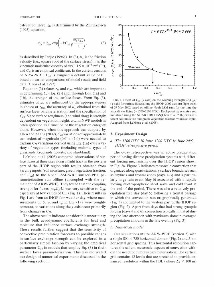
LeMone et al. (2008) compared observations of sur-
face fluxes at three sites along a flight track in the western
part of the IHOP region with results obtained from
varying inputs (soil moisture, green vegetation fraction,
and Czil) to the Noah LSM–WRF surface–PBL pa-
rameterization run offline (uncoupled with the re-
mainder of ARW-WRF). They found that the coupling
strength for fluxes, rcpCHU, was very sensitive to Czil,
especially at low values of Czil (Fig. 1). Their results in
Fig. 1 are from an IHOP fair-weather day, where mea-
surements of U, r, and cp in Eq. (1a) were roughly
constant, so variations along the y axis occur primarily
from changes in CH.
The above results indicate considerable uncertainty
in the bulk aerodynamic coefficients for heat and
moisture that influence surface exchange strength.
These results further suggest that the sensitivity of
convective precipitation forecasts to possible ranges
in surface exchange strength can be explored in a
particularly simple fashion by varying the empirical
parameter Czil in models that employ Eq. (3) in their
surface layer parameterization. This has motivated
our design of numerical experiments discussed in the
following section.
3. Experiment Design
a. The 1200 UTC 10 June–1200 UTC 16 June 2002IHOP retrospective period
The 6-day retrospective was an active precipitation
period having diverse precipitation systems with differ-
ent forcing mechanisms over the IHOP region shown
in Fig. 2a. Figure 3 indicates mesoscale convection that
organized along quasi-stationary surface boundaries such
as drylines and frontal zones (days 1–3) and a particu-
larly large rain event (day 6) associated with a rapidly
moving midtropospheric short wave and cold front at
the end of the period. There was also a relatively pre-
cipitation free day (day 5) following a frontal passage
in which the convection was orographically generated
(Fig. 3) and limited to the western part of the IHOP re-
gion (Fig. 2). Apart from days that had strong synoptic
forcing (days 4 and 6), convection typically initiated dur-
ing the late afternoon with maximum domain-averaged
precipitation amounts in the late evening (Fig. 3).
b. Numerical model
Our simulations utilize ARW-WRF (version 2) with
a single 800 3 750 horizontal domain (Fig. 2) and 3-km
horizontal grid spacing. This horizontal resolution cap-
tures the salient mesoscale aspects of convection with-
out the need for cumulus parameterization. The vertical
grid contains 42 levels that are stretched to provide en-
hanced resolution within the PBL (where Dz , 100 m)
FIG. 1. Effect of Czil (x axis) on the coupling strength rcpCHU
( y axis) for surface fluxes along the IHOP_2002 western flight track
of 29 May 2002 based on offline Noah LSM runs for the time the
aircraft was flying (;1700–2100 UTC). Each point represents a run
initialized using the NCAR HRLDAS(Chen et al. 2007) with dif-
ferent soil moisture and green vegetation fraction values as input.
Adapted from LeMone et al. (2008).
FEBRUARY 2011 T R I E R E T A L . 5
Page 4
and ;1-km spacing at the model top near 50 hPa. All
simulations use the Thompson et al. (2008) bulk micro-
physical parameterization, which predicts cloud water,
cloud ice, rain, snow, and graupel hydrometeor species.
Other physical parameterizations include the Rapid
Radiative Transfer Model (RRTM) longwave (Mlawer
et al. 1997) and Dudhia (1989) shortwave radiation
schemes.
FIG. 2. (a) Map of USGS 24-category land use over the model domain for simulations de-
scribed in section 3. Land use categories that do not occur over the simulation domain are
marked with an asterisk in the legend at right. The white inner rectangle denotes the IHOP
region of interest in the current study. This is the region for which area averages in Fig. 3 are
computed. (b) Values of Czil (see text) for the simulations where it is a function of the vege-
tation types in (a) through Eq. (4). Both S2 and S9 are the locations of IHOP surface flux
stations where corresponding model output is compared in Fig. 5.
6 W E A T H E R A N D F O R E C A S T I N G VOLUME 26
Page 5
The PBL parameterization (Janjic 1990, 1994, 2001)
used in our primary simulations, referred to hereafter as
the Mellor–Yamada–Jancic (MYJ) PBL scheme, pre-
dicts turbulent kinetic energy (TKE) and governs ver-
tical mixing between model layers. Local forcing of TKE
is provided by shear production, buoyancy production,
and dissipation terms. Horizontal mixing is determined
using a Smagorinsky first-order closure discussed in 4.1.3
of Skamarock et al. (2005).
The initial conditions for ARW-WRF are obtained
from the National Centers for Environmental Predic-
tion (NCEP) Environmental Data Assimilation Sys-
tem (EDAS) analyses, which have a horizontal grid
spacing of ;40 km. Lateral boundary conditions with a
3-h frequency are generated from corresponding opera-
tional Eta Model for the same times.
This atmospheric model is coupled with the Noah
LSM (Ek et al. 2003). The LSM has a single vegetation
canopy layer and predicts volumetric soil moisture and
temperature in four soil layers. The depths of the soil
layers are sequentially 0.1, 0.3, 0.6, and 1.0 m. The root
zone is contained in the upper 1 m (top-three layers).
The initial land surface conditions are supplied by the
NCAR high-resolution land surface data assimilation sys-
tem (HRLDAS). HRLDAS (Chen et al. 2007) is run
offline but on the same 3-km horizontal grid as the ARW-
WRF simulations for an 18-month spinup period prior to
each forecast. This land surface initialization uses a vari-
ety of observed and analyzed conditions including the
following: 1) the National Weather Service (NWS) Office
of Hydrology Stage 4 rainfall data on a 4-km national grid
(Fulton et al. 1998); 2) 0.58 hourly downward solar radia-
tion derived from Geostationary Operational Environmen-
tal Satellite-8 and -9 (GOES-8 and GOES-9) as described
by Pinker et al. (2002); 3) near-surface atmospheric tem-
perature, humidity, wind, downward longwave radiation,
and surface pressure from 3-hourly EDAS analyses; 4)
1-km horizontal resolution U.S. Geological Survey (USGS)
24-category land use and 1-km horizontal resolution state
soil geographic soil texture maps; and 5) 0.158 monthly
satellite-derived green vegetation fraction based on 5-yr
averages (Gutman and Ignatov 1997).
c. Simulations
We analyze sets of simulations designed to examine the
effect of the strength of the surface heat–moisture ex-
change on daytime PBL evolution, convection initiation,
and 0–24-h QPF over the IHOP region. A set of three
experiments (Table 1) use constant values of Czil and span
a range of values consistent with results from empirical
FIG. 3. Time series of Stage 4 precipitation observations during the 6-day IHOP_2002
retrospective period area averaged over the inner rectangular region in Fig. 2. The domi-
nant forcings are annotated for indicated events. The darker annotations and arrows in-
dicate the specific three cases examined in section 5. Local daylight time (LDT) over this
region is UTC – 5 to 6 h.
TABLE 1. List of numerical simulations discussed in the paper.
Czil Parameter Value PBL scheme Remarks
Strong surface exchange 0.01 MYJ All 6 days
Weak surface exchange 1.0 MYJ All 6 days
WRF default 0.1 MYJ All 6 days
Variable surface exchange Function of vegetation type according to Eq. (4) MYJ All 6 days
Strong surface exchange 0.01 YSU Day 5 only
Weak surface exchange 1.0 YSU Day 5 only
FEBRUARY 2011 T R I E R E T A L . 7
Page 6
studies (Chen et al. 1997; Chen and Zhang 2009). These
include simulations with Czil 5 0.01 and Czil 5 1.0, which
are respectively referred to as the strong surface exchange
and weak surface exchange runs. Simulations with the
standard Czil value used in recent versions of ARW-WRF
of 0.1 are referred to as the WRF default runs. We analyze
a fourth set of simulations where Czil varies across the
domain as a function of momentum roughness length,
Czil
5 10�4.0z0m , (4)
based on empirical relationships between vegetation types
and CH discussed in Chen and Zhang (2009). These sim-
ulations are referred to as the variable surface exchange
runs (Table 1). Over most of the IHOP region, the variable
Czil lies between the WRF default value of 0.1 and the
weak exchange value of 1.0 (Fig. 2b). These relatively large
Czil values are consistent with the relatively small rough-
ness lengths of the dominant grassland, cropland, and
shrubland vegetation types (Fig. 2a). In urban areas and in
some forested regions near the edges of the IHOP sub-
domain (Fig. 2a), including the Ozark Mountains and the
eastern edge of the Rocky Mountains, Czil values are ap-
proximately at or less than the strong exchange value of
0.01 (Fig. 2b).
It should be noted, however, that even in the constant
Czil runs, CH varies spatially, primarily through its de-
pendence on z0m (2), which is a function of vegetation
category. These interdomain variations of CH for the
constant Czil runs are still much less than those that oc-
cur in simulations in which Czil is allowed to vary ac-
cording to (4). Each of the four sets of simulations with
different specifications of Czil (and thus CH) comprise
24-h forecasts initialized at 1200 UTC for each of the six
individual days of the retrospective period (section 3a).
To explore possible sensitivities to forecast length and
initialization time, 12–36-h forecasts initialized at
0000 UTC were compared to their 0–24-h counterparts
(i.e., same valid times) initialized at 1200 UTC.
The effects of surface exchange strength on the evolu-
tion of the daytime PBL and subsequent precipitation can
be influenced by the choice of model PBL parameteriza-
tion. We explore this sensitivity by performing simulations
that use the Yonsei University (YSU) PBL scheme but are
FIG. 4. (a) Volumetric soil moisture in the top 0.1-m layer,
(b) surface sensible heat flux, and (c) surface latent heat flux at
1900 UTC (1300–1400 LDT) 14 Jun 2002 for the simulation in
which Czil is based on vegetation type (section 3c). The IHOP
surface flux stations S2 and S9 for which simulated and observed
fluxes are presented in Fig. 5 are annotated as in Fig. 2. The W and
E partitioned rectangles denote subdomains for area averages
presented in subsequent figures and discussed in the text.
8 W E A T H E R A N D F O R E C A S T I N G VOLUME 26
Page 7
otherwise identical to the strong (Czil 5 0.01) and weak
(Czil 51.0) coupling runs described above (Table 1). In
contrast to the MYJ PBL scheme, the YSU scheme (Noh
et al. 2003; Hong et al. 2006) allows nonlocal vertical mix-
ing. Comparisons are made with the MYJ simulations for
day 5 (1200 UTC 14 June–1200 UTC 15 June). On this day,
afternoon cloudiness was less widespread than on other
days, which affords a cleaner comparison of surface ex-
change effects on the afternoon PBL and subsequent pre-
cipitation. The general lack of clouds over the IHOP region
on this day is reflected in the widespread strong early af-
ternoon surface fluxes (Figs. 4b and 4c).
4. Sensitivity to surface exchange strengthand comparison with observations
a. Comparison of simulated surface fluxes and PBLwith local IHOP measurements
The simulated and observed fluxes at selected IHOP
surface flux stations on day 5 (Fig. 5) represent the transition
from predominately sensible H to latent LE fluxes from
west to east across the IHOP region (cf. Figs. 4b and 4c).
Though representativeness issues can complicate model
comparisons with individual observation sites, the selec-
tion of stations with similar observed and model land use
types (grasslands) and cloudless conditions may mitigate
such difficulties to some degree. A model comparison with
station S2 (Fig. 5a) suggests a positive bias in the strength
of simulated H in the western IHOP region, with values
from the weak surface exchange run most closely matching
observations. In contrast, the observed LE lies in the
middle of the range of simulated LE at both the western
and eastern edges of the region (Figs. 5b and 5d). Here, the
variable surface exchange run agrees remarkably well with
the observations at each of these stations, which span a
wide range of soil wetness in the simulations (Fig. 4a).
The much greater total surface flux H 1 LE in the
strong surface exchange run than in the weak surface
exchange run (Fig. 5) implies substantial differences in
the surface energy budget, Rnet 5 H 1 LE 1 G, where
Rnet is the net radiation gain (including incoming and
FIG. 5. (a)–(d) Comparisons of observed and simulated surface fluxes at IHOP surface flux station locations S2 and
S9 (locations shown in Figs. 2 and 4) for the daytime and evening portion of day 5 (1300 UTC 14 Jun to 0400 UTC
15 Jun) of the STEP IHOP_2002 retrospective period. The model land use categories (Fig. 2a) for stations 2 and 9 are
grassland/crop mosaic and grassland, respectively. LDT is UTC 2 5 h.
FEBRUARY 2011 T R I E R E T A L . 9
Page 8
reflected shortwave and outgoing longwave), and G is
the flux into the ground. For example, at S2 midday
H 1 LE is ;300 W m22 greater in the strong surface
exchange run than in the weak surface exchange run
(Figs. 5a and 5b), with ;150 W m22 less G, which
contributes to a lower skin temperature (DTs ; 220 K)
and smaller outgoing longwave radiation that increases
Rnet by ;150 W m22. Together, the differences in G
and Rnet approximately balance those in H 1 LE.
The westernmost station (S2 in Fig. 4) approximately
coincides with the IHOP Homestead sounding site
(Weckwerth et al. 2004) and thereby allows us to ex-
amine the impact of local surface fluxes on the afternoon
clear convective boundary layer and evaluate how well
this interaction is simulated at this location. More
comprehensive studies of the observed PBL evolution
on this day are found in Couvreux et al. (2009) and
Bennett et al. (2010).
Figure 6 presents observations and the simulated PBL
structure at our extremes of surface exchange strength
(Czil 5 0.01 and Czil 5 1.0) for day 5. The PBL thermal
and moisture structures for the other simulations vary
relatively smoothly between those of the simulations us-
ing our extremes, particularly for potential temperature
(not shown). Although the weak surface exchange run
(Czil 5 1.0 with MYJ PBL) produces fluxes that closely
match the observations (Fig. 6c), the associated PBL is
;500 m too shallow and ;3 K too cool (Fig. 6a),
whereas the strong surface exchange run (Czil 5 0.01
with MYJ PBL) has a PBL depth and potential tem-
perature similar to the observations (Fig. 6a) despite
much stronger than observed H (Fig. 6c). These com-
parisons suggest that the vertical mixing in the MYJ
PBL scheme may not be aggressive enough at this par-
ticular location.
A simulation with strong surface exchange and the
YSU PBL scheme (Czil 5 0.01 with YSU PBL) produces
a warmer and deeper PBL than with MYJ (Fig. 6a)
despite slightly smaller H (Fig. 6c). Here, the too warm
and too deep YSU PBL is more consistent with the too
large simulated H (Figs. 6a and 6c) than is the better
represented PBL using MYJ. Although the differences
in potential temperature among runs with different PBL
schemes can be significant, these differences are much
FIG. 6. Simulated and observed (a) potential temperature and (b) water vapor mixing ratio in the early afternoon
(1930 UTC) of day 5 (14 June) at the Homestead sounding site, which is approximately collocated with the IHOP
surface flux station S2, whose location is depicted in Figs. 2 and 4. Simulated and observed (c) surface sensible heat
flux and (d) surface latent heat flux at station S2 for the daytime surface heating cycle that approximately precedes the
vertical soundings in (a) and (b). LDT is UTC 2 5 h.
10 W E A T H E R A N D F O R E C A S T I N G VOLUME 26
Page 9
smaller than those between runs for which Czil is equal to
0.01 and 1.0 (Fig. 6a). This is not the case for the PBL
moisture, where the choice of PBL scheme makes
a larger difference than for potential temperature, par-
ticularly when the surface exchange is strong (Fig. 6b).
Acting alone, the larger LE associated with stronger
surface exchange (Fig. 6d) promotes greater PBL mois-
ture. However, because of the very dry conditions above
the PBL at this location (Fig. 6b), particularly deep ver-
tical mixing occurs with strong surface exchange for the
more aggressive YSU PBL scheme, leading to the driest
PBL of all four simulations (Fig. 6b). This deeper and
drier simulated daytime PBL using the YSU versus MYJ
PBL scheme is consistent with results over the western
high plains from previous studies (Weisman et al. 2008).
b. Regional comparison of PBL variables
Figure 7 presents a comparison of PBL variables in the
primary MYJ simulations with the Rapid Update Cycle
(RUC) model (Benjamin et al. 2004) analyses for the full
diurnal cycle averaged over the 6-day retrospective pe-
riod within the broader IHOP subdomain regions shown
FIG. 7. Comparison of gridded RUC analyses with simulations of PBL quantities for 6-day averages of 0–24-h
forecasts initialized at 1200 UTC and area-averaged over the (a),(c),(e) western and (b),(d),(f) eastern sub-
domains depicted in Fig. 4. The vertical lines indicate approximate average noon and midnight LDT over the
different averaging areas.
FEBRUARY 2011 T R I E R E T A L . 11
Page 10
in Fig. 4. Here, we select RUC analyses as a proxy for
observations since they both assimilate more observa-
tions at asynoptic times than do the corresponding EDAS
analyses used to initialize the ARW-WRF simulations
(section 3b), and they are considered more independent
from these simulations. The mean diurnal cycles of po-
tential temperature and water vapor mixing ratio (Figs.
7a–d) are interpolated from the simulation and RUC
analyses grids to 100 m AGL. This height is above day-
time superadiabatic surface layers so that conditions are
more representative of the PBL.
Over the western subdomain (Fig. 4), the magnitude
of the diurnal cycle of potential temperature (Fig. 7a)
and water vapor (Fig. 7c) in the WRF default and strong
surface exchange simulations compare best with those of
the RUC analyses. The much weaker diurnal cycle in the
weak surface exchange runs (Figs. 7a and 7c) is consistent
FIG. 8. Comparisons of Stage 4 precipitation observations with
simulated area-averaged hourly precipitation rates over the (a)
western and (b) eastern subdomains depicted in Fig. 4 for 6-day
averages of 0–24-h forecasts initialized at 1200 UTC. The vertical
lines indicate approximate average noon and midnight LDT over
the different averaging regions.
FIG. 9. Comparisons of Stage 4 precipitation observations with
simulated area-averaged hourly precipitation rates over the entire
IHOP region depicted by the solid rectangles in Fig. 4 for 6-day
averages of (a) 0–24-h forecasts initialized at 1200 UTC and (b) 12–
36-h forecasts initialized at 0000 UTC but valid for the same times
as those in (a). (c) Equitable threat scores for simulated 3-h pre-
cipitation amounts calculated over the same IHOP region and
averaged for the six 0–24-h (12–36-h) forecasts initialized at 1200
(0000) UTC. The vertical lines indicate approximate average noon
and midnight LDT over the IHOP region.
12 W E A T H E R A N D F O R E C A S T I N G VOLUME 26
Page 11
with the shallower daytime PBL (Fig. 7e). The shallower
PBL and its lesser vertical mixing in the weak surface
exchange simulations contributed to a significantly cooler
average afternoon PBL over this broad region than in
observations (Fig. 7a), as found for the Homestead site on
day 5 (Fig. 6a).
The cooler average PBL and its shallower depth in
weaker surface exchange runs also occur over the east-
ern subdomain (Figs. 7b and 7f). However, in this region
where LE exceeds H (Figs. 4b and 4c), the differences
among simulations are less pronounced than over the
west. One important difference between the two regions
is that the strong surface exchange runs have a drier
afternoon PBL than weak surface exchange runs in the
west (Fig. 7c), whereas the opposite is true in the east
(Fig. 7d). We attribute this regional difference in water
vapor evolution among simulations to stronger vertical
mixing of dry air into the PBL due to large sensible heat
flux differences in the west (e.g., Fig. 5a), whereas large
latent heat flux differences (e.g., Figs. 5d and 5f) domi-
nate in the east.
c. Regional comparison of simulated and observedprecipitation
Over the western subdomain, afternoon and evening
6-day-average precipitation rates are largest for the sim-
ulations with stronger surface exchange (Fig. 8a). The
average onset of precipitation in the strong surface ex-
change runs also occurs ;2 h earlier than for the weak
surface exchange runs (Fig. 8a), consistent with the more
rapid growth of the daytime PBL (Fig. 7e). Average pre-
cipitation rates from the variable surface exchange runs
most closely match those from Stage 4 precipitation
observations (Fig. 8a), consistent with the best agreement
of simulated to average RUC-analyzed 100-m moisture
values around the time of afternoon convection initiation
at t 5 9–12 h (Fig. 7c).
Average precipitation rates over the eastern subdo-
main (Fig. 8b) are larger than over the western subdomain
FIG. 10. The convective inhibition (gray shading) and the level of
the maximum negative buoyancy DTmin (white line) for condi-
tionally unstable PBL air parcels. The pressure at the top of the
PBL is denoted by pi. Adapted from Crook (1996).
FIG. 11. RUC analysis of 850-hPa winds, temperature (dashed
contours, with 2.58C contour interval), dewpoint (8C, scale at right),
and geopotential height (solid contours, with 30-m contour in-
terval). The rectangle denotes the IHOP analysis region.
FIG. 12. Equitable threat scores for simulated 3-h precipitation
amounts calculated over the rectangular IHOP region in Figs. 11 and 13
for 0–24-h forecasts initialized at 1200 UTC 11 Jun 2002. The vertical
lines denote average local daylight times over the region as in Fig. 9.
FEBRUARY 2011 T R I E R E T A L . 13
Page 12
(Fig. 8a). Over the eastern subdomain, smaller average
afternoon and evening precipitation rates in the weak sur-
face exchange runs are similar to the western subdomain,
however, the delayed onset of daytime precipitation rela-
tive to the strong surface exchange runs is less evident.
The pronounced afternoon minimum in observed pre-
cipitation in the eastern subdomain was not replicated
by any of the sets of 0–24-h simulations (Fig. 8b). This
shortcoming of the simulations is likely influenced by
model spinup issues because the final stages of nocturnal
convection that commonly occur over this latitude band
near sunrise (e.g., Carbone et al. 2002) cannot be well sim-
ulated using a 1200 UTC initialization. Previous studies
using convection-resolving versions of ARW-WRF have
had success in simulating this daytime minimum in central
plains precipitation when the model is run continuously
over multiple diurnal cycles (e.g., Trier et al. 2006, 2010).
Differences in the 6-day-average simulated diurnal cy-
cle of precipitation over the entire IHOP region (Fig. 2) are
evident in a comparison between the 0–24- (Fig. 9a) and
12–36-h forecasts valid at the same times (Fig. 9a). For
instance, the 12–36-h forecasts have greater postsunrise
morning precipitation and a smaller evening maximum
than do the 0–24-h forecasts. The 12–36-h forecasts
have an afternoon precipitation minimum also found
in the observations (though much stronger in the model)
that was missed in the 0–24-h forecasts, presumably be-
cause of the previously noted model spinup issues in the
1200 UTC initializations.
Unlike for forecast length and initialization time, the
surface exchange strength does not fundamentally alter the
simulated diurnal cycle of precipitation (Figs. 9a and 9b).
However, differences related to surface exchange strength
occur in both the 0000 (12–36-h forecasts) and 1200 UTC
(0–24-h forecasts) initializations. These include greater late
afternoon–evening area-averaged precipitation (by up to
40%–100%) and an earlier onset (by up to 1–3 h) for strong
compared to weak surface exchange (Figs. 9a and 9b).
Although some attributes of the 12–36-h forecasts, in-
cluding the area-averaged afternoon precipitation mini-
mum, may appear more realistic than their counterparts
from the 0–24-h forecasts, their average skill as measured
by the equitable threat score (ETS; Rogers et al. 1996) for
3-h precipitation totals is considerably less (Fig. 9c). This
likely reflects the greater difficulty in precisely forecasting
FIG. 13. Three-hour precipitation amounts for simulations with
(a) weak and (b) strong surface exchange during t 5 10–13 h and
(c) observed (Stage 4) precipitation amounts for the same period.
The rectangles denote the region over which equitable threat
scores of simulated 3-h precipitation amounts are presented for the
entire 0–24-h forecast period (Fig. 12) of day 2.
14 W E A T H E R A N D F O R E C A S T I N G VOLUME 26
Page 13
the location of precipitation at longer lead times. In both
the 0–24- and 12–36-h forecasts, despite substantial dif-
ferences in area-averaged precipitation rates, the 6-day-
average ETS differences among simulations of different
surface exchange strength are modest (Fig. 9c). However,
individual cases from the 0–24-h forecasts discussed in the
next section reveal larger forecast skill differences among
these simulations under specific circumstances.
5. Case studies
The previous section highlights sensitivity of average
precipitation rates to differences in the evolution of the
daytime PBL for sets of simulations with different surface
exchange strengths. In the current section, we examine in
more detail how the surface exchange strength influences
the timing of local deep CI and subsequent evolution of
precipitation for three cases with different synoptic forcing.
Critical to the differences in CI onset are differences in
the convection inhibition energy (CIN) that conditionally
unstable air parcels originating in the daytime PBL must
overcome to reach their level of free convection (LFC).
The CIN is illustrated schematically by the gray shading
in Fig. 10. CIN, however, is undefined at locations where
a parcel LFC is absent [i.e., where zero convective
available potential energy (CAPE) exists], which can re-
sult in discontinuities that pose a drawback to its spatial
analysis. Alternatively, we can examine a continuous field
FIG. 14. Analyses at 2000 UTC (;1500 LDT) 11 Jun 2002 for simulations using different Czil values. (a),(b) Surface
winds, regions exceeding 30-dBZ reflectivity (bold black contours), smoothed surface water vapor mixing ratio (thin
black contours), and CAPE of the most unstable (i.e., maximum equivalent potential temperature) 500-m deep air
parcel. (c),(d) Surface winds, regions exceeding 30-dBZ reflectivity (red contours), smoothed surface potential
temperature (yellow contours), and maximum negative buoyancies of the most unstable parcel. The arrows in each
panel highlight regions discussed in the text.
FEBRUARY 2011 T R I E R E T A L . 15
Page 14
approximating the CIN by using the maximum temper-
ature deficit (DTmin) of the most unstable lifted air parcel
of 500-m depth. The most unstable parcels can occur at
any level below ;3 km AGL, but for the current appli-
cation of daytime CI they originate in the PBL.
The location of DTmin for a lifted PBL parcel is in-
dicated by the white line in Fig. 10, and its value is given
by the departure of the lifted parcel temperature from
the environmental temperature. Note that the relation-
ship between CIN and DTmin is analogous to the re-
lationship between CAPE and the minimum lifted index
for air parcels with positive buoyancy. In the forth-
coming analysis, we make use of fields of both DTmin and
CAPE to illustrate effects of surface exchange on CI.
a. Day 2 (1200 UTC 11 June–1200 UTC 12 June)CI along quasi-stationary boundaries
Day 2 of the retrospective period was characterized
by late afternoon and early evening development of me-
soscale clusters of deep convection along a surface front
in Kansas and more isolated convection along a dryline
(Cai et al. 2006; Wakimoto and Murphey 2010) that trailed
southwestward into the Texas panhandle and southeast
New Mexico. The 1200 UTC 11 June 850-hPa RUC
analyses (Fig. 11) show very moist conditions ahead of the
baroclinic zone, which moved slowly southeastward within
the IHOP region during the day.
The ETS for this case indicates that the weak surface
exchange run has the best afternoon and early evening
QPF skill (Fig. 12). It is clear from comparing patterns
of forecasted 3-h precipitation amounts (Figs. 13a and
13b) with observations (Fig. 13c) that the reduced late
afternoon and evening (t 5 12–16 h) ETS in the strong
surface exchange run (Fig. 12) results primarily from
overforecasting the spatial extent of the precipitation.
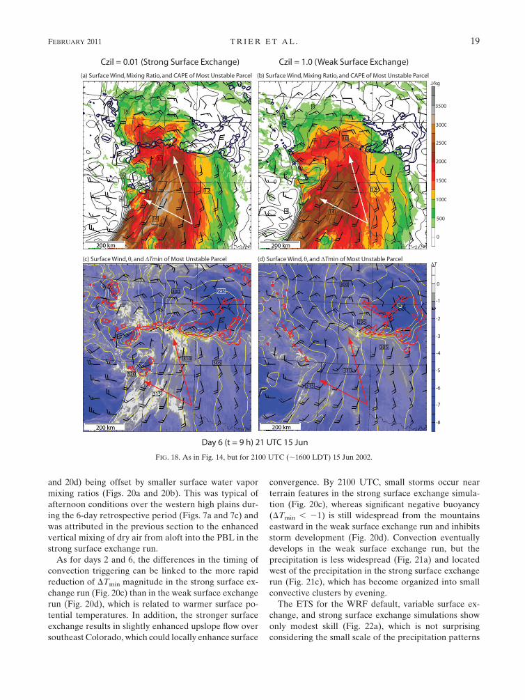
Figure 14 presents midafternoon CAPE and DTmin for
the weak and strong surface exchange runs. Other sim-
ulations for this day and other cases had features in-
termediate between these extremes of surface exchange
and are not presented. By midafternoon, CAPE is about
500–1000 J kg21 larger in the strong surface exchange
run for regions highlighted by the arrows (Figs. 14a and
14b). Since CAPE in these locations is large (2000–
4000 J kg21) in both simulations, the differences in DTmin
(Figs. 14c and 14d) are likely more critical to differences in
the timing of CI and perhaps the subsequent precipitation
amounts. In particular, narrow bands of reduced DTmin
magnitude appearing in the strong surface exchange run
(Fig. 14c) are absent in the weak surface exchange run
(Fig. 14d). These bands, which extend along the leading
edge of the surface front from Kansas into northwest
Oklahoma (northeasternmost two arrows) and within
the dryline moisture gradient in southeast New Mexico
(southwesternmost arrow), are consistent with more widely
forecasted precipitation within these and nearby regions
during the next 2–5 h (Figs. 13a and 13b).
The reduction in DTmin along the leading edge of the
surface front in the strong surface exchange run results
from both 0.5–1.0 g kg21 greater moisture (cf. Figs. 14a
and 14b) and 0–2.5 K warmer potential temperatures
(cf. Figs. 14c and 14d), whereas within the dryline moisture
gradients it is due entirely to the 2.5–5 K warmer condi-
tions (cf. Figs. 14c and 14d).
In contrast to the cold front and dryline zones, there
are also broad regions of small DTmin magnitude located
in southern Missouri and northern Arkansas in both
simulations (Figs. 14c and 14d) where little subsequent
precipitation occurs (Figs. 13a and 13b) despite sub-
stantial CAPE (Figs. 14a and 14b). This indicates that
vanishing DTmin magnitude (and similarly vanishing CIN)
is not a sufficient condition for CI. In the absence of sig-
nificant convergence, factors inhibiting deep convection
that are not considered by parcel theory including dry-air
entrainment and downward-directed pressure forces within
updrafts may be more important (e.g., Trier 2003). In the
current case, CI is mostly limited to persistent mesoscale
convergence zones. However, the CI is clearly modulated
by the strength of the surface–atmosphere heat and mois-
ture exchange.
b. Day 6 (1200 UTC 15 June–1200 UTC 16 June)squall line associated with a mobile short wave
The heaviest area-averaged precipitation event of the
retrospective period occurred on the sixth and final day
FIG. 15. RUC analysis of 700-hPa winds, temperature (dashed
contours, with 2.58C contour interval), and geopotential height
(solid contours, with 30-m contour interval). The rectangle denotes
the IHOP analysis region. The bold-dashed line indicates the po-
sition of the translating midtroposheric short wave.
16 W E A T H E R A N D F O R E C A S T I N G VOLUME 26
Page 15
(Fig. 3). The large-scale environment in its advance (Fig. 15)
consisted of a southeastward-moving midtrospheric short
wave along with strong warm advection, which together
implied favorable quasigeostrophic forcing for ascent over
the western part of the IHOP domain.
The initial formation of a mesoscale convective system
(MCS) during the morning (Fig. 16g) is well forecasted
by both the weak (Fig. 16a) and strong (Fig. 16d) surface
exchange simulations. The success of all simulations in
capturing the timing and location of the initial CI is re-
vealed by large ETS for 3–6-h precipitation forecasts of
;0.5 (Fig. 17). The lack of sensitivity to surface exchange
strength in the onset of the precipitation event differs
from the previously discussed case. This aspect along
FIG. 16. As in Fig. 13, but for the (a),(d),(g) 3–6-, (b),(e),(h) 7–10-, and (c),(f),(i) 15–18-h periods of 0–24-h forecasts of day 6. The
annotations 1 and 2 in (e) and (h) highlight precipitation features discussed in the text. The rectangles denote the region over which equitable
threat scores and bias of simulated 3-h precipitation amounts are presented for the entire 0–24-h forecast period (Fig. 17) of day 6.
FEBRUARY 2011 T R I E R E T A L . 17
Page 16
with the onset of precipitation relatively early in the di-
urnal cycle (prior to 1800 UTC) indicates a more domi-
nant role of forced ascent on CI.
Differences in the forecasted 3-h precipitation amounts
do eventually develop where, in contrast to the previous
case (Fig. 12), there is greater skill in evening forecasts (t 5
12–18 h) for the stronger surface exchange runs (Fig. 17).
Their superiority in this case can be traced to two aspects
beginning in the early-to-midafternoon.
The first is the observed development of precipitation
within the MCS westward of 1008W denoted by feature 1
(Fig. 16h) being captured by the strong surface exchange
run (Fig. 16e) while it is delayed in the weak surface
exchange run (Fig. 16b). In both the weak and strong
surface exchange runs, a moist tongue within surface
southwesterly flow contributes to large CAPE upstream
of the western part of the MCS (Figs. 18a and 18b).
However, the potential temperatures are ;2.5 K warmer
with comparable moisture in the strong surface exchange
run (northeastern arrows in Fig. 18). These differences
in potential temperature contribute to a more rapid re-
duction in the magnitude of DTmin along the southwest
edge of the MCS gust front in the strong surface exchange
run, which promotes triggering of new convection cor-
responding to feature 1 of Fig. 16 that has yet to occur in
the weak surface exchange run (cf. Figs. 18c and 18d).
The second difference concerns the observed after-
noon development of smaller convective clusters over
elevated terrain to the southwest denoted by feature 2
(Fig. 16h), which is captured by the strong surface ex-
change run (Fig. 16e) but is missed by the weak surface
exchange run (Fig. 16b). A large region of small negative
buoyancy (jDTminj , 1 K) denoted by the southwestern-
most arrow in the strong surface exchange run (Fig. 18c),
which is absent in the weak surface exchange run (Fig. 18d),
supports growth of this terrain-induced convection
(Fig. 18c) as it drifts slowly southeastward. Several hours
later the terrain-induced convection merges with the
more rapidly southward moving convection along the
MCS gust front (not shown), leading to similar evening
positions and orientations of the southwestern leading
edge of the MCS precipitation shield in the observations
(Fig. 16i) and the strong surface exchange run (Fig. 16f).
This interaction of these two different components of
afternoon convection is not well simulated by the weak
surface exchange run, and the result is a slower south-
ward progression and modified orientation of the fore-
casted evening MCS precipitation (cf. Figs. 16c and 16i).
c. Day 5 (1200 UTC 14 June –1200 UTC 15 June)orographically forced CI
The precipitation over the IHOP region on day 5 was
the lightest and least widespread of any of the retrospec-
tive days (Fig. 3) because of unfavorable synoptic forcing
associated with a midtropospheric ridge at the west edge
of the region (Fig. 19). The precipitation that did occur
was confined to a relatively narrow north–south corridor
over which southeasterly (upslope) surface flow restored
limited amounts of moisture into east-central and south-
east Colorado (Figs. 20a and 20b). Unlike the previous
two cases, there were no mesoscale boundaries or large-
scale forcing to focus convection, so CI was dependent on
smaller-scale terrain-induced convergence.
Modest CAPE of ;250–1250 J kg21 was limited to
the region of positive horizontal moisture advection,
and in contrast to days 2 and 6 was nearly equal in the
weak and strong surface exchange runs (Figs. 20a and
20b). The nearly equal CAPE in the current case can be
explained by the warmer midafternoon surface potential
temperatures in the strong surface exchange run (Figs. 20c
FIG. 17. (a) Equitable threat score and (b) bias for simulated 3-h
precipitation amounts calculated over the rectangular IHOP re-
gion in Figs. 15 and 16 for 0–24-h forecasts initialized at 1200 UTC
15 Jun 2002. The vertical lines denote average local daylight times
over the region as in Fig. 9.
18 W E A T H E R A N D F O R E C A S T I N G VOLUME 26
Page 17
and 20d) being offset by smaller surface water vapor
mixing ratios (Figs. 20a and 20b). This was typical of
afternoon conditions over the western high plains dur-
ing the 6-day retrospective period (Figs. 7a and 7c) and
was attributed in the previous section to the enhanced
vertical mixing of dry air from aloft into the PBL in the
strong surface exchange run.
As for days 2 and 6, the differences in the timing of
convection triggering can be linked to the more rapid
reduction of DTmin magnitude in the strong surface ex-
change run (Fig. 20c) than in the weak surface exchange
run (Fig. 20d), which is related to warmer surface po-
tential temperatures. In addition, the stronger surface
exchange results in slightly enhanced upslope flow over
southeast Colorado, which could locally enhance surface
convergence. By 2100 UTC, small storms occur near
terrain features in the strong surface exchange simula-
tion (Fig. 20c), whereas significant negative buoyancy
(DTmin , 21) is still widespread from the mountains
eastward in the weak surface exchange run and inhibits
storm development (Fig. 20d). Convection eventually
develops in the weak surface exchange run, but the
precipitation is less widespread (Fig. 21a) and located
west of the precipitation in the strong surface exchange
run (Fig. 21c), which has become organized into small
convective clusters by evening.
The ETS for the WRF default, variable surface ex-
change, and strong surface exchange simulations show
only modest skill (Fig. 22a), which is not surprising
considering the small scale of the precipitation patterns
FIG. 18. As in Fig. 14, but for 2100 UTC (;1600 LDT) 15 Jun 2002.
FEBRUARY 2011 T R I E R E T A L . 19
Page 18
during this period of unfavorable synoptic forcing (Fig. 19).
However, the forecast skill in these simulations repre-
sents an improvement over that of the weak surface ex-
change run, which demonstrates no skill (Fig. 22a). The
lesser skill of the weak surface exchange run in the cur-
rent case is accompanied by a strong bias toward too little
precipitation throughout the period (Fig. 22b), which is
a consequence of the PBL experiencing too little daytime
growth and warming.
For this day we examined the relationship between
precipitation and the land–atmosphere exchange for an
additional set of simulations that utilized the YSU PBL
scheme. Here, we find that the choice of PBL scheme
does not fundamentally alter the role of surface exchange
strength on precipitation; namely, that the stronger sur-
face exchange results in heavier precipitation that initiates
earlier and therefore has a leading edge that advances
eastward more rapidly (cf. Figs. 21a and 21c with Figs. 21b
and 21d). Precipitation amounts are, however, significantly
influenced by the different PBL schemes. In particular,
the simulations that use YSU produce less precipitation
in high plains locales (Fig. 21), which may be partly re-
lated to deeper vertical mixing reducing afternoon PBL
moisture in YSU (relative to MYJ) as discussed earlier
for upstream afternoon soundings (Fig. 6b).
6. Summary and discussion
In this study, we examine the sensitivity of the day-
time PBL and precipitation in a cloud-resolving at-
mospheric model (ARW-WRF) to the parameterized
surface–atmosphere exchange strength for a 6-day con-
vectively active period during IHOP_2002 field phase.
The surface exchange strength in the model was influ-
enced by varying the Zilitinkevich (1995) coefficient Czil
in Eq. (3), which is typically set to a domainwide constant
value, through a range representative of maximum and
minimum derived values (e.g., Chen and Zhang 2009).
These numerical experiments established sensitivity
of both the timing of deep convective precipitation and
area-averaged precipitation amounts to prescribed Czil
values. Simulations were compared with IHOP obser-
vations of the fluxes and daytime fair-weather PBL and
more widespread PBL and precipitation properties de-
termined from gridded model-based analyses and Stage
4 precipitation analyses for the entire 6-day retrospec-
tive. Here, the observations for the most part intersected
the broad range of possible responses from the simula-
tions with different surface exchange strengths.
The surface exchange strength does not fundamentally
alter the general location of mesoscale precipitation sys-
tems and overall characteristics of their forecasted diurnal
cycle, which contrasts with other sensitivities explored
in the study including model initialization time. However,
both 6-day averages and a more detailed examination of
individual cases revealed that simulations with strong
surface exchange (Czil 5 0.01) systematically produced
precipitation that both initiated up to several hours
earlier and had greater amounts than in corresponding
simulations with weak surface exchange (Czil 5 1.0). The
quicker onset and larger precipitation amounts in the
strong surface exchange runs were linked to more rapid
growth and warming of the daytime PBL owing to en-
hanced surface sensible heat flux. The simulations that
used Czil 5 0.1, the default value in the current versions
of ARW-WRF, produced both a quicker onset of pre-
cipitation and larger overall amounts than observed in
6-day averages, suggesting that the surface exchange may
be somewhat too strong.
These model sensitivities of precipitation to surface
exchange strength appear comparable or even greater
than those in previous studies of land surface–atmosphere
interaction where different land surface models were used
(e.g., Trier et al. 2008) and initial land surface conditions
including the specificity of soil wetness (e.g., Trier et al.
2008) and green vegetation fraction (e.g., James et al.
2009) were varied. Examination of a particular case in
the current study that lacked large-scale forcing (day 5)
suggests that effects of the surface exchange strength on
precipitation could also be comparable or greater than
those associated with the choice of PBL scheme. Thus,
being able to properly account for uncertainties in the
surface exchange strength could be potentially benefi-
cial for some forecasting applications.
Precipitation sensitivity to surface exchange strength
was greatest over the high plains part of the IHOP region
located west of ;1008W longitude. This may be due in part
to drier soils in these locations having a greater influence
3000
3060
3120
3180
3120 3060
10
10
5
5
5
0
0
0
15
1200 UTC 14 Jun (Day 5) 700-hPa RUC Analysis
FIG. 19. As in Fig. 15, but for 1200 UTC 14 Jun 2002.
20 W E A T H E R A N D F O R E C A S T I N G VOLUME 26
Page 19
on enhancements of the sensible heat flux H differences
among simulations. For dry soils, the temperature dif-
ference Ts 2 T in (1a) is larger than for wetter soils. When
Czil is increased, the bulk aerodynamic coefficient for heat
and moisture CH is reduced, which reduces H. This in-
creases Ts and hence Ts 2 T partially compensate the re-
duction in CH. For larger initial values of Ts 2 T (dry soils),
the fractional impact of this compensation is less, which
allows greater H changes.
Concepts from the parcel theory of conditional insta-
bility were applied to three diverse precipitation events
during the retrospective period to illustrate in greater de-
tail the role of surface exchange strength in daytime con-
vection initiation. The more rapid convection initiation in
the strong surface exchange simulations is primarily due to
the earlier removal of negative buoyancy for conditionally
unstable PBL air parcels. Although the stronger surface
exchange can enhance CAPE and reduce the negative
buoyancy through input of both heat and moisture into the
PBL, it is the associated potential temperature increases
that appear most crucial to these convection initiation tim-
ing differences. This was most evident over the western part
of the IHOP region, where deeper vertical mixing results in
greater PBL drying during the day than in weak surface
exchange runs despite increased moisture input from the
surface. Forecasted precipitation differences among simu-
lations with different surface exchange strength can occur
from the onset of convective triggering (e.g., days 2 and 5),
while in cases with strong large-scale forcing they may not
develop until much later as MCSs mature (e.g., day 6).
FIG. 20. As in Fig. 14, but for 2100 UTC (;1600 LDT) 14 Jun 2002.
FEBRUARY 2011 T R I E R E T A L . 21
Page 20
For 6-day averages over the western part of the IHOP
region, precipitation forecasts using variable Czil, which
depended on vegetation type (heights) through assigned
momentum roughness lengths (e.g., Chen and Zhang
2009), most closely followed the Stage 4 observations
both in timing of convection initiation and overall amounts.
Thus, allowing the surface exchange strength to vary
based on properties of the vegetation indicates the po-
tential promise for more realistic operational forecasts
of precipitation in this convection-triggering region.
FIG. 21. Three-hour precipitation amounts for simu-
lations (a)–(d) with different combinations of PBL
scheme (columns) and surface exchange strength (rows)
during t 5 12–15 h of the day 4 forecasts, and (e) ob-
served (Stage 4) precipitation amounts for the same
period. The rectangles denote the region over which
equitable threat scores of simulated 3-h precipitation
amounts are presented for the entire 0–24-h forecast
period (Fig. 22) of day 5. The cross symbol indicates the
location of the Homestead sounding site from which
observed and simulated PBL profiles from earlier in the
afternoon are presented in Figs. 6a,b.
22 W E A T H E R A N D F O R E C A S T I N G VOLUME 26
Page 21
Farther east (i.e., east of 1008W), the advantage of
using variable Czil was less evident. We speculate that
one possible reason for these geographical differences is
that a sizeable fraction of the convection over the central
plains originates from upstream and are perhaps more
likely to be strongly influenced by cumulative errors from
other model parameterizations. Clearly, the systematic
variability of surface exchange effects on precipitation
over the IHOP region alone indicates the need for ad-
ditional studies that investigate the applicability of the
current results for both different locations and for other
seasons.
A major impediment to the accurate representation of
surface exchange in operational models is the uncer-
tainty in the roughness length for heat and moisture z0t.
Allowing Czil to vary in Eq. (3), as was done in the cur-
rent study, is an expedient way to strongly influence z0t
and thereby examine the sensitivity of precipitation to
a broad range of surface exchange strengths. However,
other factors including how the roughness length for
momentum z0m is specified and the accuracy of the
friction velocity u*
calculation also influence z0t and the
surface exchange. More research is needed to discern
how best to determine z0t in operational models using
Eq. (3) or other techniques (e.g., Brutsaert 1982).
As future research stimulates improvements in the
parameterization of surface exchange, additional work
will likely be required to optimally translate such im-
provements into increased QPF skill. This is because
errors in surface exchange combine with other sources
of model error to influence PBL and precipitation fore-
casts. Frameworks that allow for assessment of the per-
formance of combinations of multiple components of a
modeling system on forecasts (e.g., Santanello et al. 2009)
may be helpful in this regard.
Acknowledgments. The authors thank Chris Davis
(NCAR) for supplying software for the negative buoy-
ancy calculations presented in section 5. Mukul Tewari
(NCAR) and Jimy Dudhia (NCAR) are acknowledged
for their help with software to run the sensitivity simu-
lations with YSU PBL scheme. The authors are grateful
to Juanzhen Sun (NCAR) for her review of an earlier
edition of this manuscript and to Chris Anderson (Iowa
State University) and two anonymous reviewers for their
constructive comments and suggestions. This work was
performed as part of NCAR’s Short Term Explicit Pre-
diction (STEP) Program, which is supported by the Na-
tional Science Foundation funds for the U.S. Weather
Research Program (USWRP).
REFERENCES
Beljaars, A. C. M., 1995: The parameterization of surface fluxes in
large-scale models under free convection. Quart. J. Roy. Me-
teor. Soc., 121, 255–270.
Benjamin, S. B., and Coauthors, 2004: An hourly assimilation–
forecast cycle: The RUC. Mon. Wea. Rev., 132, 495–518.
Bennett, L. J., T. M. Weckwerth, A. M. Blyth, B. Geerts, Q. Miao,
and Y. P. Richardson, 2010: Observations of the evolution of
the nocturnal and convective boundary layers and the struc-
ture of open-celled convection on 14 June 2002. Mon. Wea.
Rev., 138, 2589–2607.
Betts, A. K., and J. H. Ball, 1995: The FIFE surface diurnal cycle
climate. J. Geophys. Res., 100, 25 679–25 693.
Brutsaert, W. A., 1982: Evaporation into the Atmosphere. Reidel,
299 pp.
Cai, H., W.-C. Lee, T. M. Weckwerth, C. Flamant, and H. V. Murphey,
2006: Observations of the 11 June dryline during IHOP_2002
A null case for convection initiation. Mon. Wea. Rev., 134,336–354.
Carbone, R. E., J. D. Tuttle, D. A. Ahijevych, and S. B. Trier, 2002:
Inferences of predictability associated with warm season
precipitation episodes. J. Atmos. Sci., 59, 2033–2056.
Chen, F., and Y. Zhang, 2009: On the coupling strength between the
land surface and the atmosphere: From viewpoint of surface
FIG. 22. (a) Equitable threat score and (b) bias for simulated 3-h
precipitation amounts calculated over the rectangular IHOP re-
gion in Figs. 19 and 21 for 0–24-h forecasts initialized at 1200 UTC
14 Jun 2002.
FEBRUARY 2011 T R I E R E T A L . 23
Page 22
exchange coefficients. Geophys. Res. Lett., 36, L10404, doi:
10.1029/2009GL037980.
——, Z. I. Janjic, and K. E. Mitchell, 1997: Impact of atmospheric
surface layer parameterization in the new land surface scheme
of the NCEP mesoscale Eta numerical model. Bound.-Layer
Meteor., 85, 391–421.
——, and Coauthors, 2007: Evaluation of the characteristics of the
NCAR high-resolution land data assimilation system during
IHOP_2002. J. Appl. Meteor. Climatol., 46, 694–713.
Couvreux, F., F. Guichard, P. H. Austin, and F. Chen, 2009: Nature
of the mesoscale boundary layer height and water vapor var-
iability observed on 14 June 2002 during the IHOP_2002
campaign. Mon. Wea. Rev., 137, 414–432.
Crook, N. A., 1996: The sensitivity of moist convection forced by
boundary layer processes to low-level thermodynamic fields.
Mon. Wea. Rev., 124, 1767–1785.
Done, J., C. A. Davis, and M. L. Weisman, 2004: The next gener-
ation of NWP: Explicit forecasts of convection using the
Weather Research and Forecasting (WRF) model. Atmos. Sci.
Lett., 5, 110–117.
Dudhia, J., 1989: Numerical study of convection observed during
the Winter Monsoon Experiment using a mesoscale two-
dimensional model. J. Atmos. Sci., 46, 3077–3107.
Ek, M. B., K. E. Mitchell, Y. Lin, E. Rogers, P. Grummann,
V. Koren, G. Gayno, and J. D. Tarpley, 2003: Implementation
of Noah land surface model advances in the NCEP opera-
tional mesoscale Eta model. J. Geophys. Res., 108, 8851,
doi:10.1029/2002JD003296.
Fritsch, J. M., and R. E. Carbone, 2004: Improving quantitative
precipitation forecasts in the warm season: A USWRP research
and development strategy. Bull. Amer. Meteor. Soc., 85, 955–
965.
Fulton, R. A., J. P. Breidenbach, D.-J. Seo, D. A. Miller, and
T. O’Bannon, 1998: The WSR-88D rainfall algorithm. Wea.
Forecasting, 13, 377–395.
Gutman, G., and A. Ignatov, 1997: Satellite-derived green vege-
tation fraction for the use in numerical weather prediction
models. Adv. Space Res., 19, 477–480.
Holt, T. R., D. Niyogi, F. Chen, K. W. Manning, M. A. LeMone,
and A. Qureshi, 2006: Effect of land–atmosphere interactions
on the IHOP 24–25 May 2002 convection case. Mon. Wea.
Rev., 134, 113–133.
Hong, S.-Y., Y. Noh, and J. Dudhia, 2006: A new vertical diffusion
package with an explicit treatment of entrainment processes.
Mon. Wea. Rev., 134, 2318–2341.
James, K. A., D. J. Stensrud, and N. Yussouf, 2009: Value of real-
time vegetation fraction to forecasts of severe convection in
high-resolution models. Wea. Forecasting, 24, 187–210.
Janjic, Z. I., 1990: The step-mountain coordinate: Physical package.
Mon. Wea. Rev., 118, 1429–1443.
——, 1994: The step-mountain Eta coordinate: Further develop-
ment of the convection, viscous sublayer, and turbulent clo-
sure schemes. Mon. Wea. Rev., 122, 927–945.
——, 1996a: The surface layer in the NCEP Eta model. Preprints,
11th Conf. on Numerical Weather Prediction, Norfolk, VA,
Amer. Meteor. Soc., 354–355.
——, 1996b: The surface layer parameterization in the NCEP Eta
model. Research Activities in Atmospheric and Oceanic Model-
ling, World Meteorological Organization, 4.16–4.17.
——, 2001: Nonsingular implementation of the Mellor–Yamada
Level 2.5 scheme in the NCEP Meso model. NCEP Office
Note 437, 61 pp. [Available online at http://www.emc.ncep.noaa.
gov/officenotes/newernotes/on437.pdf.]
Kain, J. S., S. J. Weiss, J. J. Levit, M. E. Baldwin, and D. R. Bright,
2006: Examination of convection-allowing configurations of
the WRF model for the prediction of severe convective weather:
The SPC/NSSL spring program 2004. Wea. Forecasting, 21,
167–181.
Koster, R. D., and Coauthors, 2004: Regions of strong coupling
between soil moisture and precipitation. Science, 305, 1138–
1140.
——, and Coauthors, 2006: GLACE: The global land–atmosphere
coupling experiment. Part I: Overview. J. Hydrometeor., 7,
590–610.
Lanicci, J. M., T. N. Carlson, and T. T. Warner, 1987: Sensitivity of
the Great Plains severe-storm environment to soil moisture
distribution. Mon. Wea. Rev., 115, 2660–2673.
LeMone, M. A., M. Tewari, F. Chen, J. G. Alfieri, and D. Niyogi,
2008: Evaluation of the Noah land surface model using data
from a fair-weather IHOP_2002 day with heterogeneous sur-
face fluxes. Mon. Wea. Rev., 136, 4915–4941.
Mlawer, E. J., S. J. Taubman, P. D. Brown, M. J. Iacono, and
S. A. Clough, 1997: Radiative transfer for inhomogeneous
atmosphere: RRTM, a validated correlated-k model for the
longwave. J. Geophys. Res., 102, 16 663–16 682.
Noh, Y., W. G. Cheon, S.-Y. Hong, and S. Raasch, 2003: Im-
provement of the K-profile model for the planetary boundary
layer based on large eddy simulation data. Bound.-Layer
Meteor., 107, 401–427.
Pielke, R. A., Sr., 2001: Influence of the spatial distribution of
vegetation and soils on the prediction of cumulus convection
rainfall. Rev. Geophys., 39, 151–177.
——, and M. Segal, 1986: Mesoscale circulations forced by differ-
ential terrain heating. Mesoscale Meteorology and Forecasting,
P. S. Ray, Ed., Amer. Meteor. Soc., 516–548.
Pinker, R. T., I. Laszlo, J. D. Tarpley, and K. Mitchell, 2002: Geo-
stationary satellite products for surface energy balance models.
Adv. Space Res., 30, 2427–2432.
Rogers, E., and Coauthors, 1996: Changes to the operational
‘‘early’’ Eta analysis/forecast system at the National Centers
for Environmental Prediction. Wea. Forecasting, 11, 391–413.
Santanello, J. A., Jr., C. D. Peters-Lidard, S. V. Kumar, C. Alonge,
and W.-K. Tao, 2009: A modeling and observational framework
for diagnosing local land–atmosphere coupling on diurnal time
scales. J. Hydrometeor., 10, 577–599.
Segal, M., and R. W. Arritt, 1992: Nonclassical mesoscale circula-
tions caused by sensible heat flux gradients. Bull. Amer. Me-
teor. Soc., 73, 1593–1604.
Skamarock, W. C., J. B. Klemp, J. Dudhia, D. O. Gill, D. M. Barker,
W. Wang, and J. G. Powers, 2005: A description of the Ad-
vanced Research WRF version 2. NCAR Tech. Note TN-
4681STR, 88 pp.
Thompson, G., P. R. Field, R. M. Rasmussen, and W. D. Hall, 2008:
Explicit forecasts of winter precipitation using an improved
bulk microphysics scheme. Part II: Implementation of a new
snow parameterization. Mon. Wea. Rev., 136, 5095–5115.
Trier, S. B., 2003: Convective storms: Convective initiation. En-
cyclopedia of Atmospheric Sciences, Academic Press, 560–
570.
——, F. Chen, and K. W. Manning, 2004: A study of convection
initiation in a mesoscale model using high-resolution land
surface initial conditions. Mon. Wea. Rev., 132, 2954–2976.
——, C. A. Davis, D. A. Ahijevych, M. L. Weisman, and
G. H. Bryan, 2006: Mechanisms supporting long-lived episodes
of propagating nocturnal convection within a 7-day WRF model
simulation. J. Atmos. Sci., 63, 2437–2461.
24 W E A T H E R A N D F O R E C A S T I N G VOLUME 26
Page 23
——, F. Chen, K. W. Manning, M. A. LeMone, and C. A. Davis, 2008:
Sensitivity of the PBL and precipitation in 12-day simulations of
warm-season convection using different land surface models and
soil wetness conditions. Mon. Wea. Rev., 136, 2321–2343.
——, C. A. Davis, and D. A. Ahijevych, 2010: Environmental con-
trols on the simulated diurnal cycle of warm-season precipitation
in the continental United States. J. Atmos. Sci., 67, 1066–1090.
Wakimoto, R. M., and H. V. Murphey, 2010: Frontal and radar
refractivity analyses of the dryline on 11 June 2002 during
IHOP. Mon. Wea. Rev., 138, 228–241.
Weckwerth, T. M., and Coauthors, 2004: An overview of the In-
ternational H2O Project (IHOP_2002) and some preliminary
highlights. Bull. Amer. Meteor. Soc., 85, 253–277.
Weisman, M. L., C. Davis, W. Wang, K. W. Manning, and J. B. Klemp,
2008: Experiences with 0–36-h explicit convective forecasts with
the WRF-ARW model. Wea. Forecasting, 23, 407–437.
Zilitinkevich, S., 1995: Non-local turbulent transport: Pollution dis-
persion aspects of coherent structure of convective flows. Air
Pollution Theory and Simulation, H. Power et al., Eds., Vol. 1,
Air Pollution III, Computational Mechanics Publications, 53–60.
FEBRUARY 2011 T R I E R E T A L . 25