70
EFFECTS OF THE BUSINESS CYCLE ON SOCIAL INDICATORS IN LATIN AMERICA AND THE CARIBBEAN: WHEN DREAMS MEET REALITY SEMIANNUAL REPORT • OFFICE OF THE REGIONAL CHIEF ECONOMIST • APRIL 2019
EFFECTS OF THE BUSINESS CYCLEON SOCIAL INDICATORS
IN LATIN AMERICA AND THE CARIBBEAN:WHEN DREAMS MEET REALITY
SEMIANNUAL REPORT • OFFICE OF THE REGIONAL CHIEF ECONOMIST • APRIL 2019

Effects of the Business Cycle on Social Indicators in Latin America and the Caribbean:
When Dreams Meet Reality

© 2019 International Bank for Reconstruction and Development / The World Bank 1818 H Street NW, Washington DC 20433 Telephone: 202-473-1000; Internet: www.worldbank.org
Some rights reserved
1 2 3 4 22 21 20 19
This work is a product of the staff of The World Bank with external contributions. The findings, interpretations, and conclusions expressed in this work do not necessarily reflect the views of The World Bank, its Board of Executive Directors, or the governments they represent. The World Bank does not guarantee the accuracy of the data included in this work. The boundaries, colors, denominations, and other information shown on any map in this work do not imply any judgment on the part of The World Bank concerning the legal status of any territory or the endorsement or acceptance of such boundaries.
Nothing herein shall constitute or be considered to be a limitation upon or waiver of the privileges and immunities of The World Bank, all of which are specifically reserved.
Rights and Permissions
This work is available under the Creative Commons Attribution 3.0 IGO license (CC BY 3.0 IGO) http://creativecommons.org/licenses/by/3.0/igo. Under the Creative Commons Attribution license, you are free to copy, distribute, transmit, and adapt this work, including for commercial purposes, under the following conditions:
Attribution—Please cite the work as follows: Végh, Carlos A., Guillermo Vuletin, Daniel Riera-Crichton, Jorge Puig,
José Andrée Camarena, Luciana Galeano, Luis Morano, and Lucila Venturi. 2019. “Effects of the Business Cycle on Social
Indicators in Latin America and the Caribbean: When Dreams Meet Reality” LAC Semiannual Report (April), World Bank,
Washington, DC. Doi: 10.1596/978-1-4648-1413-6. License: Creative Commons Attribution CC BY 3.0 IGO
Translations—If you create a translation of this work, please add the following disclaimer along with the attribution: This translation was not created by The World Bank and should not be considered an official World Bank translation. The World Bank shall not be liable for any content or error in this translation.
Adaptations—If you create an adaptation of this work, please add the following disclaimer along with the attribution: This is an adaptation of an original work by The World Bank. Responsibility for the views and opinions expressed in the adaptation rests solely with the author or authors of the adaptation and are not endorsed by The World Bank.
Third-party content—The World Bank does not necessarily own each component of the content contained within the work. The World Bank therefore does not warrant that the use of any third-party-owned individual component or part contained in the work will not infringe on the rights of those third parties. The risk of claims resulting from such infringement rests solely with you. If you wish to re-use a component of the work, it is your responsibility to determine whether permission is needed for that re-use and to obtain permission from the copyright owner. Examples of components can include, but are not limited to, tables, figures, or images.
All queries on rights and licenses should be addressed to the Publishing and Knowledge Division, The World Bank, 1818 H Street NW, Washington, DC 20433, USA; fax: 202-522-2625; e-mail: [email protected].
ISBN (electronic):978-1-4648-1413-6 DOI: 10.1596/978-1-4648-1413-6 Cover design: Javier Daza.
| 3
Acknowledgements
This report was prepared by a core team from the Office of the Chief Economist, Latin America and
the Caribbean, composed of Carlos A. Végh (Regional Chief Economist), Guillermo Vuletin (Senior
Economist), Daniel Riera-Crichton (Economist), Jorge Puig (Professor, UNLP, Argentina), and José
Andrée Camarena, Luciana Galeano, Luis Morano, and Lucila Venturi (Research Analysts). Members
of the World Bank’s Regional Management Team for Latin America and the Caribbean asked pointed
questions and provided invaluable insights during a presentation that took place on March 25, 2019.
Jorge Araujo, Practice Manager of Macroeconomics, Trade, and Investment, and his team of country
economists, particularly James Sampi, offered invaluable support. Oscar Calvo, Carolina Diaz-Bonilla,
María Ana Lugo, and Natalia García Peña from the Poverty and Equity Global Practice kindly
provided data support as well as helpful comments and suggestions. Our thanks to Elena
Ianchovichina, Maria Marta Ferreyra, Joana Silva, Guillermo Beylis, Jessica Bracco, Andrés César,
Guillermo Falcone, Diego Friedheim, Leonardo Gasparini, Joaquín Serrano, and Leopoldo Tornarolli
for insightful feedback. Candyce Rocha (Acting Communications Manager), Carlos Molina (Online
Communications Officer), Shane Romig, and Anahí Rama (Communications Officers) provided
constant feedback and assistance that made this report more accessible to non-economists. Finally,
this report would not have come to fruition without the unfailing administrative support of Jacqueline
Larrabure and Ruth Eunice Flores.
April 2019

4 | When Dreams Meet Reality
| 5
Executive Summary
After six years of growth deceleration (including a fall in GDP of almost 1 percent in 2016), the Latin
America and the Caribbean (LAC) region had resumed in 2017 what seemed to be a path of modest
but increasing growth, led by a rise in GDP of 1.3 percent. A pickup in oil and copper prices, large
net capital inflows into the region, modest recoveries in Argentina and Brazil, and an extremely gradual
pace of monetary policy normalization in the advanced economies, especially in the United States, all
contributed to this turnaround in 2017 and, as of last April, growth in 2018 was expected to be 1.8
percent. Unfortunately, the much-anticipated path of increasing growth was not to be, as the region
hit several bumps in the road, which reduced 2018 growth from the 1.8 percent projection to an
estimated 0.7. In particular, (i) the financial crisis that hit Argentina in April 2018 and led to a sharp
contraction in GDP of 2.5 percent in 2018, (ii) the tepid recovery in Brazil after the major recession
of 2015 and 2016, (iii) the anemic growth in Mexico in the midst of political uncertainty, and (iv) the
continuing implosion of Venezuela’s economy all turned into a perfect storm that brought growth
down in 2018 to a very modest rate of 0.7 percent. (Excluding Venezuela, growth in the region also
fell from 1.9 percent in 2017 to 1.4 in 2018.) Among the large economies of the region, Colombia
was the silver lining with a healthy growth rate of 2.7 percent.
Regrettably, and as argued in Chapter 1, growth prospects for this year (0.9 percent) show no real
improvement over 2018, as a result of weak or negative growth in the three largest economies in the
region – Brazil, Mexico, and Argentina – and a total collapse in Venezuela (with GDP projected to
fall by 25 percent). Overall, South America – which represents more than 70 percent of LAC’s output
– is expected to grow by only 0.4 percent in 2019 (1.8 percent excluding Venezuela). In contrast,
Central America and the Caribbean are expected to grow strongly at 3.4 percent and 3.2 percent,
respectively. Finally, Mexico is expected to grow by 1.7 percent (down from 2.0 in 2018), reflecting
mainly markets’ concerns about mixed signals regarding the course of future economic policy.
As is often the case, external factors will also pose a challenge for the region. The sharp drop in
commodity prices – especially oil and copper – during the last months of 2018 and the deceleration
of Chinese growth may turn into significant headwinds as the region attempts to raise its growth rate.
Oil prices are of vital importance for Colombia, Ecuador, Mexico, and Venezuela, and copper prices
for Chile and Peru. Growth in China is particularly relevant for South America as China has already
become the main commercial partner of several countries in the region, including Brazil and Peru.
On the financial side, the increase in international interest rates, mainly due to the ongoing monetary
policy normalization in the United States, has generated an appreciation of the dollar and thus put
pressure on emerging markets’ currencies. Since the region’s currencies have started to depreciate,
central banks already confront the monetary policy dilemma analyzed in previous issues of this report:

6 | When Dreams Meet Reality
raise policy interest rates to defend the currency at the cost of sacrificing growth or lower policy rates
to stimulate the economy at the cost of further depreciation and, possibly, capital outflows. Moreover,
there has been a steep drop in net capital inflows (measured as the 12-month cumulative figure), which
fell from a high of 50 billion dollars in January 2018 to virtually zero in January 2019. Having said
that, the latest announcement by the Federal Reserve of no more policy rate increases in 2019 and
only one in 2020 should provide a breather to the region.
On the fiscal front, the region continues to be in a difficult situation, while moving slowly in the right
direction. In 2019, we estimate that 27 out of 32 countries in the region will have a deficit in the
overall fiscal balance (in 2018, 29 out of 32 had an overall fiscal deficit). The median overall fiscal
deficit in the region has fallen from 2.4 percent of GDP in 2018 to 2.1 percent in 2019. In South
America, it has fallen from 3.8 percent of GDP to 2.8. Due to widespread fiscal deficits, however,
average public debt remains high for the region, at almost 60 percent of GDP, with seven countries
having debt-to-GDP ratios above 80 percent. Since January 2018, Fitch has downgraded the credit
ratings of four countries, and changed to a negative outlook the prospect for two major economies
(Argentina and Mexico). Thus, access to and cost of international credit are, once again, becoming
more challenging when most needed.
Given the mediocre growth performance of the region, in particular South America, a worsening of
social indicators should not come as a surprise. Brazil, which accounts for one-third of the region’s
population, has seen an increase in monetary poverty of approximately 3 percentage points between
2014 and 2017. The business cycle has a clear impact on social indicators, a fact often overlooked in
poverty discussions. In this light, the dramatic fall in poverty during the Golden Decade (2003-2013)
needs to be also put into context, because one would conjecture that at least some of those social
gains would be temporary (i.e., due to the extremely favorable phase of the business cycle).1 The core
of this report, Chapters 2-4, elaborates on these important ideas related to the effects of the business
cycle on social indicators, especially poverty.
Chapter 2 conveys the first key idea: not all social indicators are created equal in terms of how much
they respond to the business cycle. To this effect, we consider three widely-used social indicators –
unemployment rate, monetary poverty (5.50-dollar poverty line), and unsatisfied basic needs (UBN) –
and compute how much of their variability is explained by the cyclical component of per capita output
in LAC. In the case of the unemployment rate, 74 percent of its variability is explained by cyclical
considerations. At the other end, only 21 percent of the variance in the UBN is explained by the
business cycle. Monetary poverty falls somewhere in between, with 43 percent of its variability due
to cyclical movements in per capita output.
Intuitively, the unemployment rate is the quintessential cyclical indicator since, in models with sticky
prices/wages, it responds strongly to any monetary or real temporary shock driving the business cycle.
In contrast, UBN is an indicator comprised of structural factors (such as housing, education, and
1 While, in a slight abuse of language, the Golden Decade is typically defined as the period 2003-2013 (given that commodity prices, and oil in particular, started a sharp decline in 2014), all of our computations related to social indicators cover the period 2003-2014 to take into account that monetary poverty in LAC reached its lowest point in 2014.
| 7
sanitation), which are little affected by the business cycle. Monetary poverty responds to both
temporary shocks and structural factors. Hence, UBN would clearly be a better indicator of social
well-being because it would not depend on the vagaries of the business cycle. Monetary poverty,
however, could yield a misleading reading of the social situation because part of its decline during
booms could be reversed when the inevitable slowdown/recession comes along.
Chapter 3 focuses on the Golden Decade, a period of remarkable growth (particularly for the region’s
commodity exporters) due to extremely high commodity prices. In this period, monetary poverty
declined by about 20 percentage points. The ideas introduced in Chapter 2, however, would clearly
suggest that part of this fall was due to cyclical, rather than trend, considerations. To ascertain this,
we build upon a well-known methodology in the poverty literature and conclude that, for LAC as a
whole, 45 percent of the fall in monetary poverty during the Golden Decade was due to cyclical
factors, while the remaining 55 percent was due to trend growth and redistributive policies. Hence,
we should be careful about how to assess permanent social gains, particularly in economies where
output is highly volatile which, as shown in Chapter 2, increases the cyclical effects on social indicators.
Since redistributive factors alone accounted for about 35 percent of the fall in poverty during the
Golden Decade and have played a key role ever since, Chapter 4 takes a closer look at the main
redistributive policy: conditional cash transfers (CCTs). CCTs are, by design, “structural” social
programs aimed at reducing long-term (and inter-generational) poverty by providing cash in exchange
for investments in health and human capital accumulation. By now, most countries in the region have
sophisticated CCTs that continue to contribute to poverty reduction. In contrast, Chapter 4 discusses
the absence in many countries of social programs, such as unemployment insurance, designed to help
the poor and vulnerable during cyclical increases in poverty. Such “shock absorbers” (or cyclical
buffers) are widespread in developed countries and constitute a pending social agenda for the region.

8 | When Dreams Meet Reality
| 9
Chapter 1
Growth, Fiscal Challenges, and Poverty in the Region
Introduction
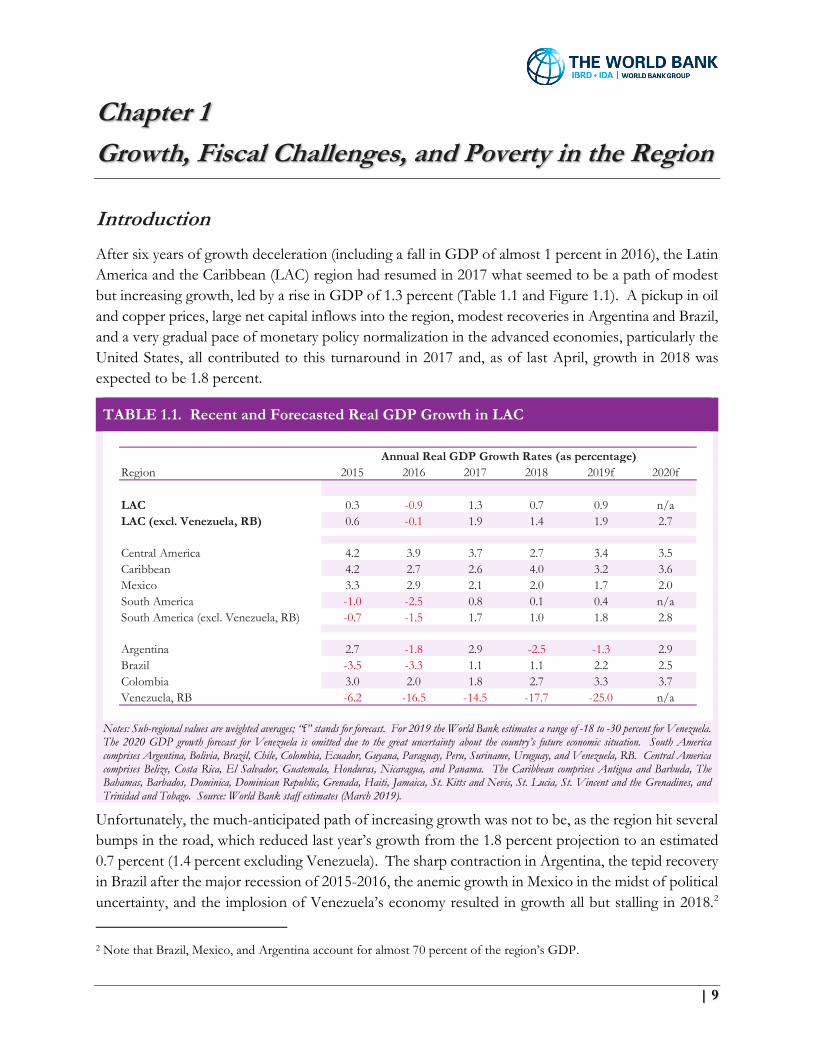
After six years of growth deceleration (including a fall in GDP of almost 1 percent in 2016), the Latin
America and the Caribbean (LAC) region had resumed in 2017 what seemed to be a path of modest
but increasing growth, led by a rise in GDP of 1.3 percent (Table 1.1 and Figure 1.1). A pickup in oil
and copper prices, large net capital inflows into the region, modest recoveries in Argentina and Brazil,
and a very gradual pace of monetary policy normalization in the advanced economies, particularly the
United States, all contributed to this turnaround in 2017 and, as of last April, growth in 2018 was
expected to be 1.8 percent.
TABLE 1.1. Recent and Forecasted Real GDP Growth in LAC
Notes: Sub-regional values are weighted averages; “f” stands for forecast. For 2019 the World Bank estimates a range of -18 to -30 percent for Venezuela. The 2020 GDP growth forecast for Venezuela is omitted due to the great uncertainty about the country’s future economic situation. South America comprises Argentina, Bolivia, Brazil, Chile, Colombia, Ecuador, Guyana, Paraguay, Peru, Suriname, Uruguay, and Venezuela, RB. Central America comprises Belize, Costa Rica, El Salvador, Guatemala, Honduras, Nicaragua, and Panama. The Caribbean comprises Antigua and Barbuda, The Bahamas, Barbados, Dominica, Dominican Republic, Grenada, Haiti, Jamaica, St. Kitts and Nevis, St. Lucia, St. Vincent and the Grenadines, and Trinidad and Tobago. Source: World Bank staff estimates (March 2019).
Unfortunately, the much-anticipated path of increasing growth was not to be, as the region hit several
bumps in the road, which reduced last year’s growth from the 1.8 percent projection to an estimated
0.7 percent (1.4 percent excluding Venezuela). The sharp contraction in Argentina, the tepid recovery
in Brazil after the major recession of 2015-2016, the anemic growth in Mexico in the midst of political
uncertainty, and the implosion of Venezuela’s economy resulted in growth all but stalling in 2018.2
2 Note that Brazil, Mexico, and Argentina account for almost 70 percent of the region’s GDP.
Region 2015 2016 2017 2018 2019f 2020f
LAC 0.3 -0.9 1.3 0.7 0.9 n/a
LAC (excl. Venezuela, RB) 0.6 -0.1 1.9 1.4 1.9 2.7
Central America 4.2 3.9 3.7 2.7 3.4 3.5
Caribbean 4.2 2.7 2.6 4.0 3.2 3.6
Mexico 3.3 2.9 2.1 2.0 1.7 2.0
South America -1.0 -2.5 0.8 0.1 0.4 n/a
South America (excl. Venezuela, RB) -0.7 -1.5 1.7 1.0 1.8 2.8
Argentina 2.7 -1.8 2.9 -2.5 -1.3 2.9
Brazil -3.5 -3.3 1.1 1.1 2.2 2.5
Colombia 3.0 2.0 1.8 2.7 3.3 3.7
Venezuela, RB -6.2 -16.5 -14.5 -17.7 -25.0 n/a
Annual Real GDP Growth Rates (as percentage)

10 | When Dreams Meet Reality
Among the large economies of the region, Colombia was the silver lining in 2018 with a healthy growth
of 2.7 percent. Regrettably, the growth prospects this year for LAC (0.9 percent) show no real
improvement over 2018, as a result of weak or negative growth in the three largest economies in the
region – Brazil, Mexico, and Argentina – and the tragic growth collapse in Venezuela.
FIGURE 1.1. Real GDP Growth in LAC
Note: Growth figures for 2019 and 2020 are forecasts. Source: World Bank staff estimates (March 2019).
Argentina starts 2019 immersed in a severe recession, with GDP projected to fall a further 1.3 percent
this year following a contraction of 2.5 percent in 2018 (Table 1.1 and Figure 1.2, Panel A). In 2018,
the peso depreciated by 66 percent relative to the previous year, inflation is still close to 50 percent,
and policy rates had to be raised above 70 percent last October to prevent further depreciation.
Despite the unprecedented support from the International Monetary Fund (IMF), reflected in a
revised package of 57.1 billion dollars in October 2018, and the central bank’s success early this year
in stabilizing the peso, the fiscal adjustment needed to comply with the IMF program is taking a heavy
toll in terms of economic activity and the peso has come under renewed attack. The government,
however, appears firmly committed to complying with the fiscal adjustment agreed with the IMF, but
the October’s presidential elections will undoubtedly test the government’s resolve.
After contracting by 3.5 and 3.3 percent in 2015 and 2016, respectively, in what is the largest recession
in thirty years, Brazil resumed positive growth in 2017 and 2018 (with GDP increasing by 1.1 percent
in both years) and is expected to grow at 2.2 percent in 2019 (Table 1.1 and Figure 1.2, Panel B). In
light of a fiscal deficit of 7.2 percent of GDP and public debt reaching almost 80 percent of GDP,
fiscal reforms in Brazil are of the essence. Pensions are, by far, the biggest fiscal burden, accounting
for close to 12 percent of GDP. To put this figure into perspective, we should note that the average
for OECD countries, which have a similar proportion of retirees, is 8 percent of GDP. On the
-3
-2
-1
0
1
2
3
4
5
6
7
Rea
l GD
P G
row
th (as
per
cent
age)
LAC LAC without Venezuela, RB
-0.9
1.30.7 0.9
-0.1
1.9
1.4
1.9
2.7
| 11
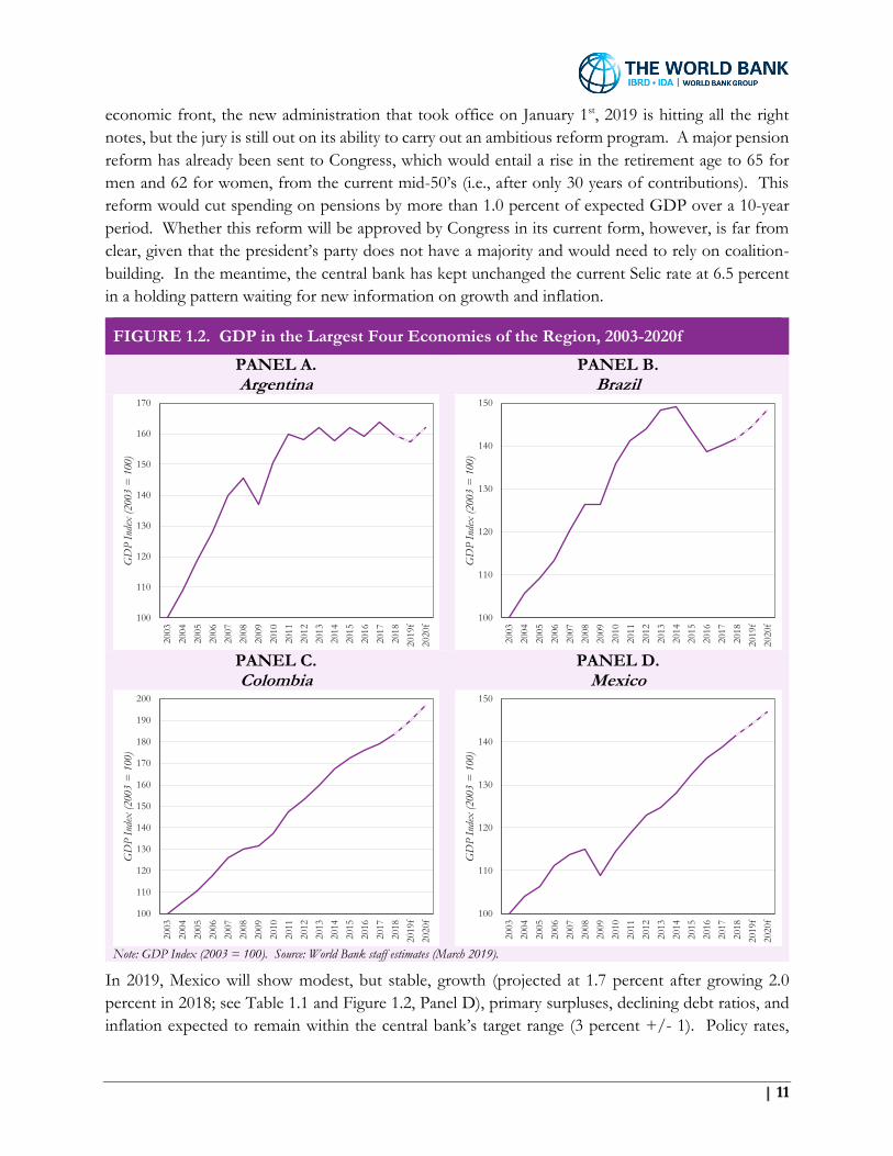
economic front, the new administration that took office on January 1st, 2019 is hitting all the right
notes, but the jury is still out on its ability to carry out an ambitious reform program. A major pension
reform has already been sent to Congress, which would entail a rise in the retirement age to 65 for
men and 62 for women, from the current mid-50’s (i.e., after only 30 years of contributions). This
reform would cut spending on pensions by more than 1.0 percent of expected GDP over a 10-year
period. Whether this reform will be approved by Congress in its current form, however, is far from
clear, given that the president’s party does not have a majority and would need to rely on coalition-
building. In the meantime, the central bank has kept unchanged the current Selic rate at 6.5 percent
in a holding pattern waiting for new information on growth and inflation.
FIGURE 1.2. GDP in the Largest Four Economies of the Region, 2003-2020f
PANEL A. Argentina
PANEL B. Brazil
PANEL C. Colombia
PANEL D. Mexico
Note: GDP Index (2003 = 100). Source: World Bank staff estimates (March 2019).
In 2019, Mexico will show modest, but stable, growth (projected at 1.7 percent after growing 2.0
percent in 2018; see Table 1.1 and Figure 1.2, Panel D), primary surpluses, declining debt ratios, and
inflation expected to remain within the central bank’s target range (3 percent +/- 1). Policy rates,
100
110
120
130
140
150
160
170
2003
2004
2005
2006
2007
2008
2009
2010
2011
2012
2013
2014
2015
2016
2017
2018
2019f
2020f
GD
P I
ndex
(20
03 =
100
)
100
110
120
130
140
150
2003
2004
2005
2006
2007
2008
2009
2010
2011
2012
2013
2014
2015
2016
2017
2018
2019f
2020f
GD
P I
ndex
(20
03 =
100
)
100
110
120
130
140
150
160
170
180
190
200
2003
2004
2005
2006
2007
2008
2009
2010
2011
2012
2013
2014
2015
2016
2017
2018
2019f
2020f
GD
P I
ndex
(20
03 =
100
)
100
110
120
130
140
150
2003
2004
2005
2006
2007
2008
2009
2010
2011
2012
2013
2014
2015
2016
2017
2018
2019f
2020f
GD
P I
ndex
(20
03 =
100
)
12 | When Dreams Meet Reality
however, remain among the highest in the region for large economies (at 8.25 percent), reflecting the
central bank’s need to defend the peso given the mixed signals from the current administration
regarding the future course of economic policies. Even before taking office, the current president
spooked markets by announcing the suspension of an already partially built 13 billion dollars new
Mexico City airport. Major energy reforms by the previous administration have been put on hold as
well, calling into question the future of Mexico’s energy policy. On the other hand, the current
administration submitted a relatively prudent fiscal budget for 2019, which was approved by Congress
in late December 2018. To add to the positive signals, the current administration has also recently
announced a slashing of the tax rate for equity IPOs and allowed pension funds to invest in a wider
range of instruments. Signals from the new administration have thus been decidedly mixed and only
time will tell which orientation will prevail. But, in the meantime, economic policy uncertainty is likely
to force the central bank to maintain a tight monetary policy, which will hurt growth. In contrast, in
Colombia (Figure 1.2, Panel C), the policy rate of 4.25 percent should stimulate growth.
But nothing could prepare the region for the escalation of the economic, social, and humanitarian
crisis in Venezuela, by far the worst in the region’s modern history (Figure 1.3). Economic and social
conditions continue to deteriorate rapidly. Declining oil prices – and hence, production and exports
of oil – together with highly distortionary policies, from price controls to directed lending, a disorderly
fiscal adjustment, monetization of the public sector deficit, and overall economic mis-management
have led to hyperinflation, devaluation (Figure 1.3, Panel A), debt defaults, and a massive contraction
in output and consumption.3 Real GDP contracted by 17.7 percent in 2018 and is likely to fall by 25.0
percent in 2019, which would imply a cumulative fall in GDP of 60 percent since 2013 (Figure 1.3,
Panel B). The inflation rate, estimated at 1.37 million percent by the end of 2018 (a monthly rate of
121 percent), is likely to reach 10 million percent in 2019 (a monthly rate of 161 percent). Estimates
by unofficial sources suggest that poverty has reached 90 percent of the population (Figure 1.3, Panel
C).4 According to the United Nations Refugee Agency and the International Organization for
Migration (2019), the number of people leaving the country is projected to surpass 5 million by the
end of 2019 (Figure 1.3, Panel D).5
As always, the region’s overall growth (0.7 percent in 2018 and a projection of 0.9 percent for 2019)
masks a great deal of heterogeneity across different sub-regions (Table 1.1). GDP in South America
(SA) remained essentially flat in 2018 (but grew 1.0 percent excluding Venezuela) and is expected to
grow by 0.4 percent in 2019 (1.8 percent excluding Venezuela). Central America’s (CA) growth was
2.7 percent in 2018 (down from 3.7 percent in 2017), partly due to the political and economic crisis in
Nicaragua that led to a fall in GDP of 3.8 percent in 2018, compared to positive growth of 4.9 percent
in 2017 (Table A.1). Growth in CA is expected to be back to 3.4 percent in 2019. The Caribbean has
3 On the humanitarian front, hunger and disease are spreading throughout the country. Infant mortality rose to 26 per 1,000 live births in the period 2013–2017, comparable to the country’s rates in the 1980s. Crime and violence have also increased substantially, with Venezuela becoming the country with the highest homicide rate in the region (89 homicides per 100,000 inhabitants), a rate almost three times as high as that of countries at war.
4 Data from ENCOVI.
5 See World Bank (2018a) for a detailed analysis of the effects of migration.

| 13
FIGURE 1.3. Venezuela: Key Indicators
PANEL A. Exchange Rate (Black Market)
PANEL B. GDP Index
PANEL C.
Poverty Rate (Non-Official)
PANEL D. Migrants
Notes: VES stands for Venezuelan sovereign bolivar. Cumulative figures for migrants since 2015. Dashed line indicates projections. Sources: ENCOVI, Federal Reserve, UNHCR, and World Bank staff estimates (March 2019).
resumed healthy growth (4.0 percent in 2018 up from 2.6 percent in 2017) after the devastation caused
by hurricanes Irma and María in 2017 and is expected to grow by 3.2 percent in 2019.
Compared to other regions in the world, LAC has consistently underperformed. Figure 1.4 compares
the average growth rates for LAC, the rest of the world, and the rest of emerging markets excluding
China (EMs). The Golden Decade of commodity prices (2003-2013) was the only period for which
the LAC region outperformed the rest of the world. Nevertheless, note that, the Golden Decade
notwithstanding, the region has always lagged EMs. Further, the slowdown in commodity prices from
2014-2015 negatively affected LAC substantially more than the EMs, which only suffered a minor
growth deceleration. This difference was greatest in 2016, when LAC contracted by almost 1.0 percent
while the EMs grew at 3.7 percent.
0
200
400
600
800
1,000
1,200
1,400
Dec-17 Feb-18 Apr-18 Jun-18 Aug-18 Oct-18 Dec-18
VE
S/U
SD
Annual inflation reaches 1,087 percent
Annual inflation reaches 1,370,000 percent(121 percent monthly)
30
40
50
60
70
80
90
100
2013 2014 2015 2016 2017 2018 2019f
GD
P I
ndex
(20
13 =
100
)
20
40
60
80
100
2013 2014 2015 2016 2017
Hea
dcou
nt R
atio
0
1
2
3
4
5
6
2015 2017 Sep-18 Dec-18 Dec-19
Mig
rant
s (i
n m
illio
ns)
Population as of 2016 = 31 million (aprox.)5 million migrants represent 16 percent of the population

14 | When Dreams Meet Reality
FIGURE 1.4. Real GDP Growth: LAC, EMs (excl. LAC and China), and Rest of the World
Note: Sub-regional values are weighted averages. Sources: World Bank staff estimates (March 2019) and WEO (October 2018).
Figure 1.5 shows the 2019 growth forecast for each of the 32 countries of the LAC region. The
median rate of real GDP growth for the region is projected at 2.4 percent. However, we can observe
FIGURE 1.5. Real GDP Growth Forecasts in LAC per Country, 2019
Note: Sub-regional values are weighted averages. Source: World Bank staff estimates (March 2019).
-2
-1
0
1
2
3
4
5
6
2003-2013 2014-2015 2016 2017-2019f
Rea
l GD
P G
row
th (as
per
cent
age)
Rest of the World LAC EMs (excl. LAC and China)
-8
-6
-4
-2
0
2
4
6
8
Ven
ezu
ela,
RB
Nic
arag
ua
Arg
enti
na
Tri
n. an
d T
obag
o
Ecu
ado
r
Hai
ti
SA
Do
min
ica
LA
C
Bar
bad
os
Jam
aica
Mex
ico
Uru
guay
Bah
amas
Su
rin
ame
MC
C
St.
Vin
. an
d G
ren
.
Bra
zil
Bel
ize
El Sal
vad
or
An
t. a
nd
Bar
bud
a
Cost
a R
ica
Colo
mb
ia
Gu
atem
ala
St.
Luci
a
Chile
Ho
nd
ura
s
Par
aguay
Per
u
Gre
nad
a
Bo
livia
Gu
yan
a
Do
min
ican
Rep
.
Pan
ama
St.
Kit
ts a
nd
Nev
.
Rea
l G
DP
Gro
wth
(as
per
cent
age)
LAC Median 2019: 2.4%
-25

| 15
a great deal of heterogeneity within the region. St. Kitts and Nevis, Panama, and the Dominican
Republic are expected to be the three fastest growing economies. The last two, however, are the only
countries in this group that have had high growth rates during 2016-2019. At the other extreme, we
can see in Figure 1.5 the meltdown in Venezuela and recessions in Nicaragua and Argentina.
Given these differences in growth across countries, what factors may explain this phenomenon? The
next section will differentiate between external and domestic factors affecting LAC.
The Role of External Factors
From the perspective of a small open economy, as those in LAC, external factors play a fundamental
role in determining growth (Figure 1.6). Indeed, these have been decisive determinants of the
slowdown that the region experienced in the aftermath of the Golden Decade.
FIGURE 1.6. External Factors Affecting LAC Growth
PANEL A. Commodity Prices
PANEL B. China Real GDP Growth
PANEL C.
U.S. Real GDP Growth
PANEL D. Real Yield on 10-year U.S. T-Note
Note: Forecasts for 2019 included when available. Sources: Bloomberg, Haver Analytics, and World Bank Commodity Price Data (Pinksheets).
20
40
60
80
100
120
140
2003
2004
2005
2006
2007
2008
2009
2010
2011
2012
2013
2014
2015
2016
2017
2018
2019
Inde
x (
2010 =
100)
Energy Commodity Index Non-Energy Commodity Index
4
6
8
10
12
14
16
2003
2004
2005
2006
2007
2008
2009
2010
2011
2012
2013
2014
2015
2016
2017
2018
2019
Rea
l GD
P G
row
th (as
per
cent
age)
-3
-2
-1
0
1
2
3
4
5
2003
2004
2005
2006
2007
2008
2009
2010
2011
2012
2013
2014
2015
2016
2017
2018
2019
Rea
l G
DP
Gro
wth
(as
per
cent
age)
-0.5
0.0
0.5
1.0
1.5
2.0
2.5
Jan-1
3A
pr-
13
Jul-
13
Oct
-13
Jan-1
4A
pr-
14
Jul-
14
Oct
-14
Jan-1
5A
pr-
15
Jul-
15
Oct
-15
Jan-1
6A
pr-
16
Jul-
16
Oct
-16
Jan-1
7A
pr-
17
Jul-
17
Oct
-17
Jan-1
8A
pr-
18
Jul-
18
Oct
-18
Jan-1
9
Rea
l Y
ield
(as
per
cent
age)

16 | When Dreams Meet Reality
The price of commodities, growth in the United States and China, and international liquidity – as
captured by the real yield on the 10-year Treasury note – are, by and large, among the most important
external factors for the region. Figure 1.6. illustrates their recent behavior. The increasing uncertainty
regarding the future path of commodity prices and the slowdown in the Chinese growth rate pose
difficult challenges for commodity exporters in the region. In particular, as of mid-March 2019, oil
prices have dropped by 17 percent since their October 2018 high, while copper prices have fallen by
8 percent since their January 2018 high. Oil is the main export for Colombia, Ecuador, and Venezuela,
and certainly important for Mexico, while copper is the main export for Chile and Peru.
Of course, behind the recent increase in world real interest rates captured by Figure 1.6, Panel D lies
primarily the monetary policy normalization in the United States. Although quite gradual, the repeated
increases in the Federal Funds Rate since December 2015 (Figure 1.7, Panel A) have certainly helped
FIGURE 1.7. Monetary Policy in the U.S. and Financial Variables
PANEL A. Federal Funds Rate
PANEL B. U.S. Dollar Index
PANEL C. Net Capital Inflows to LAC
PANEL D. Emerging Markets’ Currency Index
Notes: Forecasts for 2019 included when available. The vertical line represents the maximum of the twelve-month-sum of net capital inflows to the LAC region. Sources: Bloomberg, EPFR Global, and Federal Reserve Board.
0.0
0.5
1.0
1.5
2.0
2.5
3.0
Jan
-13
May
-13
Sep
-13
Jan
-14
May
-14
Sep
-14
Jan
-15
May
-15
Sep
-15
Jan
-16
May
-16
Sep
-16
Jan
-17
May
-17
Sep
-17
Jan
-18
May
-18
Sep
-18
Jan
-19
May
-19
Sep
-19
Jan
-20
May
-20
Sep
-20
Jan
-21
May
-21
Sep
-21
Jan
-22
May
-22
Sep
-22
As
perc
enta
ge
70
75
80
85
90
95
100
105
Jan-1
3A
pr-
13
Jul-
13
Oct
-13
Jan-1
4A
pr-
14
Jul-
14
Oct
-14
Jan-1
5A
pr-
15
Jul-
15
Oct
-15
Jan-1
6A
pr-
16
Jul-
16
Oct
-16
Jan-1
7A
pr-
17
Jul-
17
Oct
-17
Jan-1
8A
pr-
18
Jul-
18
Oct
-18
Jan-1
9
Inde
x
-40
-30
-20
-10
0
10
20
30
40
50
60
Jan
-13
Ap
r-13
Jul-
13
Oct
-13
Jan
-14
Ap
r-14
Jul-
14
Oct
-14
Jan
-15
Ap
r-15
Jul-
15
Oct
-15
Jan
-16
Ap
r-16
Jul-
16
Oct
-16
Jan
-17
Ap
r-17
Jul-
17
Oct
-17
Jan
-18
Ap
r-18
Jul-
18
Oct
-18
Jan
-19
Bill
ions
of
dolla
rs
1,400
1,450
1,500
1,550
1,600
1,650
1,700
1,750
Jan
-13
Apr-
13
Jul-
13
Oct
-13
Jan
-14
Apr-
14
Jul-
14
Oct
-14
Jan
-15
Apr-
15
Jul-
15
Oct
-15
Jan
-16
Apr-
16
Jul-
16
Oct
-16
Jan
-17
Apr-
17
Jul-
17
Oct
-17
Jan
-18
Apr-
18
Jul-
18
Oct
-18
Jan
-19
Inde
x
| 17
in appreciating the dollar (Figure 1.7, Panel B) and, more recently, contributed to a sharp fall in net
capital inflows (measured as the 12-month cumulative figure), from a high of 50 billion dollars in
January 2018 to virtually zero in January 2019 (Figure 1.7, Panel C). Not coincidentally, this dramatic
fall in net capital inflows has been accompanied by a sharp appreciation of the dollar since January
2018 and a corresponding depreciation of emerging markets’ currencies (Figure 1.7, Panel D). The
depreciation of domestic currencies in LAC has begun to confront central banks with the monetary
policy dilemma analyzed in Végh et al. (2017). Should central banks increase policy rates to defend
domestic currencies at the cost of aggravating a possible economic slowdown, or should they lower
policy rates to stimulate the economy at the cost of further depreciation and inflation? Having said
that, the latest announcement by the Federal Reserve of no more policy rate increases in 2019 and
only one in 2020 should provide a breather to the region.
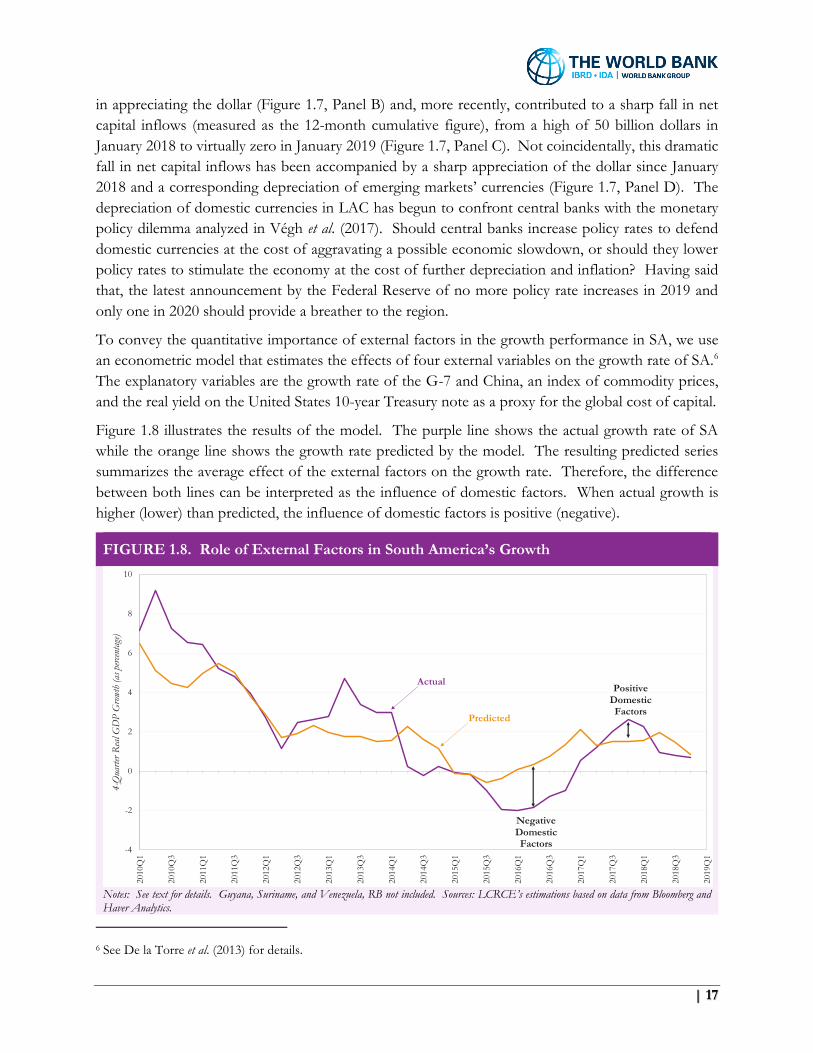
To convey the quantitative importance of external factors in the growth performance in SA, we use
an econometric model that estimates the effects of four external variables on the growth rate of SA.6
The explanatory variables are the growth rate of the G-7 and China, an index of commodity prices,
and the real yield on the United States 10-year Treasury note as a proxy for the global cost of capital.
Figure 1.8 illustrates the results of the model. The purple line shows the actual growth rate of SA
while the orange line shows the growth rate predicted by the model. The resulting predicted series
summarizes the average effect of the external factors on the growth rate. Therefore, the difference
between both lines can be interpreted as the influence of domestic factors. When actual growth is
higher (lower) than predicted, the influence of domestic factors is positive (negative).
FIGURE 1.8. Role of External Factors in South America’s Growth
Notes: See text for details. Guyana, Suriname, and Venezuela, RB not included. Sources: LCRCE’s estimations based on data from Bloomberg and Haver Analytics.
6 See De la Torre et al. (2013) for details.
-4
-2
0
2
4
6
8
10
2010Q
1
2010Q
3
2011Q
1
2011Q
3
2012Q
1
2012Q
3
2013Q
1
2013Q
3
2014Q
1
2014Q
3
2015Q
1
2015Q
3
2016Q
1
2016Q
3
2017Q
1
2017Q
3
2018Q
1
2018Q
3
2019Q
1
4-Q
uart
er R
eal G
DP
Gro
wth
(as
per
cent
age)
Actual
Predicted
NegativeDomestic Factors
Positive DomesticFactors
18 | When Dreams Meet Reality
The figure makes clear that the deceleration in the region’s growth rate since the end of the Golden
Decade of high commodity prices was driven by external factors. Additionally, it can be observed
that SA’s growth rate was notably affected by domestic factors, in particular the Brazilian recession of
2015-2016 (the largest in the country’s recent history). Currently, actual and predicted growth
coincide, which tells us that SA is generating little, if any, of its own growth and needs to urgently find
its own sources of growth, as repeatedly emphasized in this series of reports.
Fiscal Adjustment in LAC: A Progress Report
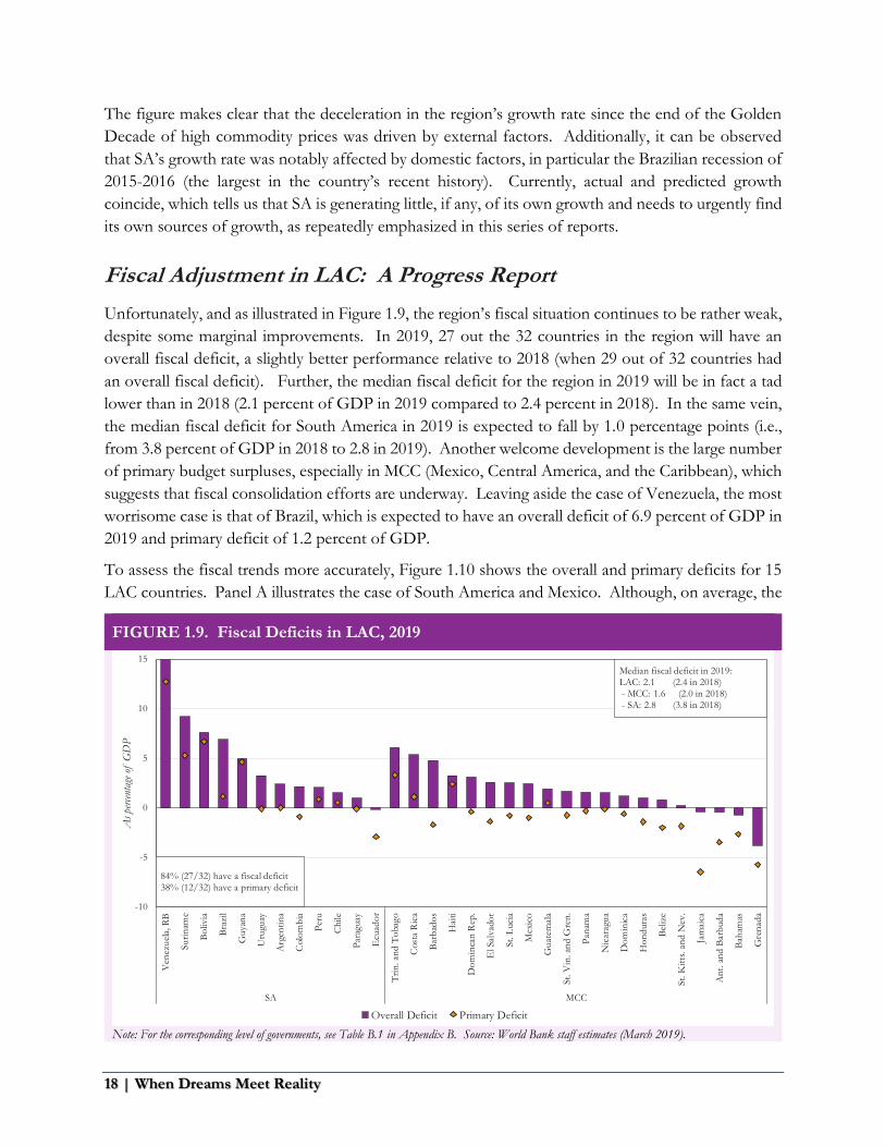
Unfortunately, and as illustrated in Figure 1.9, the region’s fiscal situation continues to be rather weak,
despite some marginal improvements. In 2019, 27 out the 32 countries in the region will have an
overall fiscal deficit, a slightly better performance relative to 2018 (when 29 out of 32 countries had
an overall fiscal deficit). Further, the median fiscal deficit for the region in 2019 will be in fact a tad
lower than in 2018 (2.1 percent of GDP in 2019 compared to 2.4 percent in 2018). In the same vein,
the median fiscal deficit for South America in 2019 is expected to fall by 1.0 percentage points (i.e.,
from 3.8 percent of GDP in 2018 to 2.8 in 2019). Another welcome development is the large number
of primary budget surpluses, especially in MCC (Mexico, Central America, and the Caribbean), which
suggests that fiscal consolidation efforts are underway. Leaving aside the case of Venezuela, the most
worrisome case is that of Brazil, which is expected to have an overall deficit of 6.9 percent of GDP in
2019 and primary deficit of 1.2 percent of GDP.
To assess the fiscal trends more accurately, Figure 1.10 shows the overall and primary deficits for 15
LAC countries. Panel A illustrates the case of South America and Mexico. Although, on average, the
FIGURE 1.9. Fiscal Deficits in LAC, 2019
Note: For the corresponding level of governments, see Table B.1 in Appendix B. Source: World Bank staff estimates (March 2019).
-10
-5
0
5
10
15
Ven
ezu
ela,
RB
Su
rin
ame
Bo
livia
Bra
zil
Gu
yan
a
Uru
guay
Arg
enti
na
Colo
mb
ia
Per
u
Chile
Par
aguay
Ecu
ado
r
Tri
n. an
d T
obag
o
Cost
a R
ica
Bar
bad
os
Hai
ti
Do
min
can
Rep
.
El Sal
vad
or
St.
Luci
a
Mex
ico
Gu
atem
ala
St.
Vin
. an
d G
ren
.
Pan
ama
Nic
arag
ua
Do
min
ica
Ho
nd
ura
s
Bel
ize
St.
Kit
ts. an
d N
ev.
Jam
aica
An
t. a
nd
Bar
bud
a
Bah
amas
Gre
nad
a
SA MCC
As
perc
enta
ge o
f G
DP
Overall Deficit Primary Deficit
84% (27/32) have a fiscal deficit38% (12/32) have a primary deficit
Median fiscal deficit in 2019:LAC: 2.1 (2.4 in 2018)- MCC: 1.6 (2.0 in 2018)- SA: 2.8 (3.8 in 2018)

| 19
FIGURE 1.10. Fiscal Deficits in Selected LAC Countries
PANEL A. South America and Mexico, 2016-2019
PANEL B. Central America and Dominican Republic, 2016-2019
Notes: “f” stands for forecast. For the corresponding level of governments, see Table B.1 in Appendix B. Source: World Bank staff estimates (March 2019).
overall deficit has improved by 2.3 percentage points and the primary deficit by 2.2 percentage points,
the figure clearly shows that fiscal consolidation efforts vary considerably across countries.
-4
-2
0
2
4
6
8
102016
2017
2018
2019f
2016
2017
2018
2019f
2016
2017
2018
2019f
2016
2017
2018
2019f
2016
2017
2018
2019f
2016
2017
2018
2019f
2016
2017
2018
2019f
2016
2017
2018
2019f
Argentina Brazil Chile Colombia Ecuador Peru Uruguay Mexico
As
perc
enta
ge o
f G
DP
Overall Deficit Primary Deficit
2016 2019f ImprovementOverall Deficit (avg.) 4.9 2.6 2.3Primary Deficit (avg.) 2.0 -0.2 2.2
-3
-2
-1
0
1
2
3
4
5
6
7
2016
2017
2018
2019f
2016
2017
2018
2019f
2016
2017
2018
2019f
2016
2017
2018
2019f
2016
2017
2018
2019f
2016
2017
2018
2019f
2016
2017
2018
2019f
Costa Rica Dominican Rep. El Salvador Guatemala Honduras Nicaragua Panama
As
perc
enta
ge o
f G
DP
Overall Deficit Primary Deficit
2016 2019f ImprovementOverall Deficit (avg.) 2.4 2.5 -0.1Primary Deficit (avg.) 0.1 -0.3 0.4
20 | When Dreams Meet Reality
Specifically, we can see consistent fiscal improvements in Argentina, Ecuador, and Peru even if, except
for Ecuador, overall deficits remain high.7 Brazil, again, stands out for its enormous overall deficit.
The picture looks less encouraging in the case of Central America and Dominican Republic (Figure
1.10, Panel B). In fact, during the four-year period 2016-2019, the average overall fiscal deficit and
primary deficit have not changed much. Further, of the seven countries in this panel, there is none
that shows consistent reductions in the overall deficit, although some countries, like El Salvador, show
repeated improvements in the primary deficit.
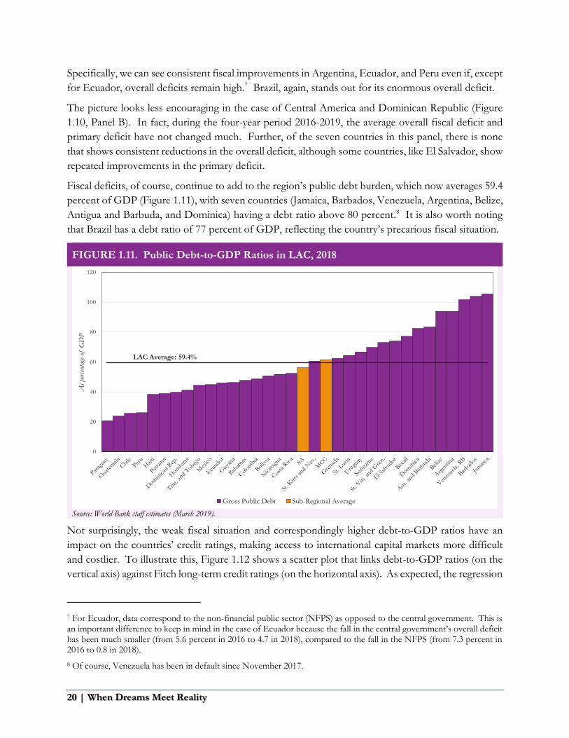
Fiscal deficits, of course, continue to add to the region’s public debt burden, which now averages 59.4
percent of GDP (Figure 1.11), with seven countries (Jamaica, Barbados, Venezuela, Argentina, Belize,
Antigua and Barbuda, and Dominica) having a debt ratio above 80 percent.8 It is also worth noting
that Brazil has a debt ratio of 77 percent of GDP, reflecting the country’s precarious fiscal situation.
FIGURE 1.11. Public Debt-to-GDP Ratios in LAC, 2018
Source: World Bank staff estimates (March 2019).
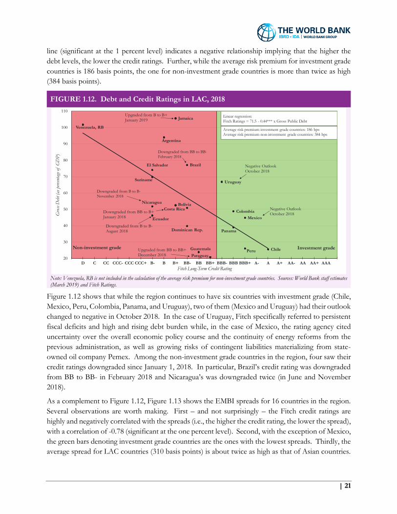
Not surprisingly, the weak fiscal situation and correspondingly higher debt-to-GDP ratios have an
impact on the countries’ credit ratings, making access to international capital markets more difficult
and costlier. To illustrate this, Figure 1.12 shows a scatter plot that links debt-to-GDP ratios (on the
vertical axis) against Fitch long-term credit ratings (on the horizontal axis). As expected, the regression
7 For Ecuador, data correspond to the non-financial public sector (NFPS) as opposed to the central government. This is an important difference to keep in mind in the case of Ecuador because the fall in the central government’s overall deficit has been much smaller (from 5.6 percent in 2016 to 4.7 in 2018), compared to the fall in the NFPS (from 7.3 percent in 2016 to 0.8 in 2018).
8 Of course, Venezuela has been in default since November 2017.
0
20
40
60
80
100
120
As
perc
enta
ge o
f G
DP
Gross Public Debt Sub-Regional Average
LAC Average: 59.4%
| 21
line (significant at the 1 percent level) indicates a negative relationship implying that the higher the
debt levels, the lower the credit ratings. Further, while the average risk premium for investment grade
countries is 186 basis points, the one for non-investment grade countries is more than twice as high
(384 basis points).
FIGURE 1.12. Debt and Credit Ratings in LAC, 2018
Note: Venezuela, RB is not included in the calculation of the average risk premium for non-investment grade countries. Sources: World Bank staff estimates (March 2019) and Fitch Ratings.
Figure 1.12 shows that while the region continues to have six countries with investment grade (Chile,
Mexico, Peru, Colombia, Panama, and Uruguay), two of them (Mexico and Uruguay) had their outlook
changed to negative in October 2018. In the case of Uruguay, Fitch specifically referred to persistent
fiscal deficits and high and rising debt burden while, in the case of Mexico, the rating agency cited
uncertainty over the overall economic policy course and the continuity of energy reforms from the
previous administration, as well as growing risks of contingent liabilities materializing from state-
owned oil company Pemex. Among the non-investment grade countries in the region, four saw their
credit ratings downgraded since January 1, 2018. In particular, Brazil’s credit rating was downgraded
from BB to BB- in February 2018 and Nicaragua’s was downgraded twice (in June and November
2018).
As a complement to Figure 1.12, Figure 1.13 shows the EMBI spreads for 16 countries in the region.
Several observations are worth making. First – and not surprisingly – the Fitch credit ratings are
highly and negatively correlated with the spreads (i.e., the higher the credit rating, the lower the spread),
with a correlation of -0.78 (significant at the one percent level). Second, with the exception of Mexico,
the green bars denoting investment grade countries are the ones with the lowest spreads. Thirdly, the
average spread for LAC countries (310 basis points) is about twice as high as that of Asian countries.
Chile
Mexico
Peru
Colombia
Panama
Uruguay
Costa Rica
Guatemala
Paraguay
Brazil
Dominican Rep.
BoliviaNicaragua
Argentina
Ecuador
Suriname
El Salvador
Venezuela, RB
Jamaica
D C CC CCC- CCC CCC+ B- B B+ BB- BB BB+ BBB- BBB BBB+ A- A A+ AA- AA AA+ AAA0
0.1
0.2
0.3
0.4
0.5
0.6
0.7
0.8
0.9
1
20
30
40
50
60
70
80
90
100
110
Gro
ss D
ebt (
as p
erce
ntag
e of
GD
P)
Fitch Long-Term Credit Rating
Linear regression:
Fitch Ratings = 71.5 - 0.44*** x Gross Public Debt
Investment gradeNon-investment gradeUpgraded from BB to BB+December 2018
Downgraded from BB to BB-
February 2018
Average risk premium investment grade countries: 186 bps
Average risk premium non-investment grade countries: 384 bps
Downgraded from B to B-
November 2018
Upgraded from B to B+January 2019
Negative OutlookOctober 2018
Downgraded from BB to B+January 2018
Downgraded from B to B-August 2018
Negative OutlookOctober 2018

22 | When Dreams Meet Reality
Finally, it should come as no surprise that the two highest spreads are for Argentina and Ecuador
(both currently under IMF programs).
FIGURE 1.13. J.P. Morgan’s EMBI Spreads
Notes: The EMBI tracks total returns for traded external debt instruments (i.e., foreign currency denominated fixed income) in emerging markets. It covers dollar-denominated Brady bonds, loans, and Eurobonds. The spread is defined as the difference between the returns of EMBI bonds and U.S. Treasury bonds, which are viewed as risk-free. Asian countries include China, India, Indonesia, Malaysia, the Philippines, and Vietnam. Bars represent average for February 2019. Source: Bloomberg.
Poverty in LAC: Trends and Cycles
Since the main focus of this report in the following chapters will be the effects of the business cycle
on various social indicators – particularly poverty – we conclude this first chapter by providing a brief
and very broad overview of poverty in the region.
As is well-known, monetary poverty reflects the share of the population below some income
threshold. Naturally, different income thresholds may be used to evaluate monetary poverty. One
commonly-used threshold is 1.9 dollars per person a day (2011 PPP), typically referred to as extreme
monetary poverty.9 As detailed in World Bank (2018b), extreme poverty stood at 10 percent of the
world’s population in 2015, down from 36 percent in 1990. While this is a remarkable feat, 10 percent
equates to 736 million people in the world still living in extreme poverty. In LAC, only 4 percent of
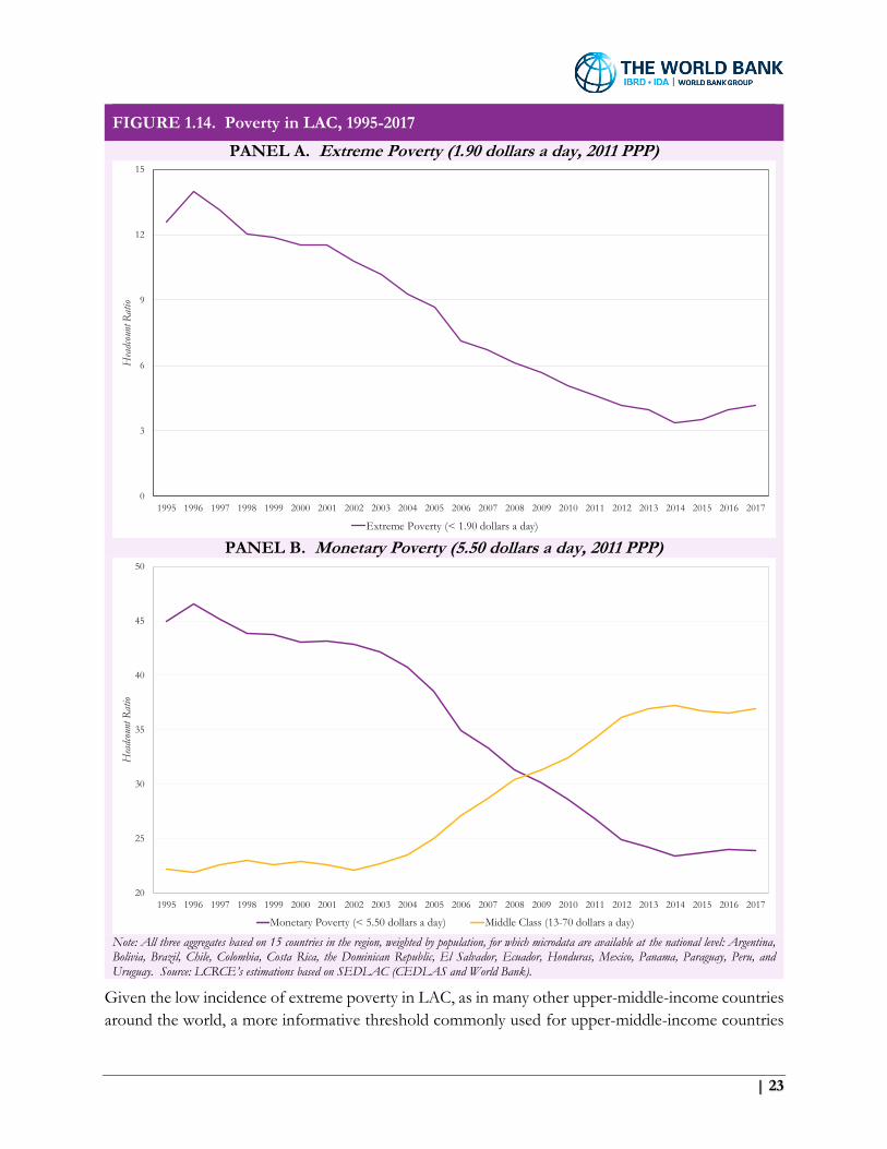
the population lives in extreme poverty. Further, as illustrated in Figure 1.14, Panel A, the reduction
in extreme poverty has been quite remarkable, falling from 13 percent in 1995 to 4 percent in 2017.
9 PPP refers to purchasing power parity; see Appendix E.
0
100
200
300
400
500
600
700
800
Bas
is P
oint
s
Investment Grade Non-Investment Grade
Average for LAC Countries: 310 bpsAverage for Asian Countries: 149 bps
LAC Average: 310 bps
Correlation(Spreads, Credit Ratings) = -0.78***
| 23
FIGURE 1.14. Poverty in LAC, 1995-2017
PANEL A. Extreme Poverty (1.90 dollars a day, 2011 PPP)
PANEL B. Monetary Poverty (5.50 dollars a day, 2011 PPP)
Note: All three aggregates based on 15 countries in the region, weighted by population, for which microdata are available at the national level: Argentina, Bolivia, Brazil, Chile, Colombia, Costa Rica, the Dominican Republic, El Salvador, Ecuador, Honduras, Mexico, Panama, Paraguay, Peru, and Uruguay. Source: LCRCE’s estimations based on SEDLAC (CEDLAS and World Bank).
Given the low incidence of extreme poverty in LAC, as in many other upper-middle-income countries
around the world, a more informative threshold commonly used for upper-middle-income countries
0
3
6
9
12
15
1995 1996 1997 1998 1999 2000 2001 2002 2003 2004 2005 2006 2007 2008 2009 2010 2011 2012 2013 2014 2015 2016 2017
Hea
dcou
nt R
atio
Extreme Poverty (< 1.90 dollars a day)
20
25
30
35
40
45
50
1995 1996 1997 1998 1999 2000 2001 2002 2003 2004 2005 2006 2007 2008 2009 2010 2011 2012 2013 2014 2015 2016 2017
Hea
dcou
nt R
atio
Monetary Poverty (< 5.50 dollars a day) Middle Class (13-70 dollars a day)

24 | When Dreams Meet Reality
is 5.50 dollars a day (2011 PPP), hereafter referred to simply as monetary poverty. Under this
definition, monetary poverty in LAC has fallen from 45 percent in 1995 to 24 percent in 2017, as
illustrated in Figure 1.14, Panel B. The counterpart of the fall in monetary poverty is the rise of the
middle class. Indeed, following Ferreira et al. (2013), we estimate that the middle class in LAC
increased from 22 percent of the population in 1995 to 37 percent in 2017 (Figure 1.14, Panel B).
Of course, these dramatic gains in terms of the reduction of both extreme and monetary poverty vary
considerably across countries, as illustrated in Figure 1.15.10 While many LAC countries have
essentially eliminated extreme poverty or reduced it way below 10 percent, it continues to be very high
in countries such as Honduras, and, particularly, Haiti. In contrast, monetary poverty is still
widespread in the region with almost two-thirds of countries (11 out of 18 in Figure 1.15) having a
poverty rate above 20 percent.
FIGURE 1.15. Latest Poverty Rates for LAC Countries
Notes: Poverty rates for the year 2017, except for Dominican Republic and Mexico (2016), Guatemala and Nicaragua (2014), and Haiti (2012). Poverty estimates based on household per capita income for all countries, except for Haiti, for which poverty rates are based on household per capita consumption. Poverty lines expressed in 2011 PPP dollars. Source: PovcalNet (March 2019).
This heterogeneity in poverty rates across countries in the region is obviously lost when regional
aggregates are considered, such as in Figure 1.14. In fact, poverty has increased sharply in some
countries in LAC since the end of the Golden Decade. In particular, Brazil, which represents one
third of the region’s population, has seen an increase in monetary poverty of about 3 percentage points
between 2014 and 2017. Figure 1.16 shows how the region’s aggregate for monetary poverty varies
10 Note that the data source for Figure 1.15 (PovcalNet, March 2019) may differ slightly for some countries compared to the rest of the report. See Appendix E for details.
0
10
20
30
40
50
60
Hea
dcou
nt R
atio
Monetary Poverty (< 5.50 dollars a day) Extreme Poverty (< 1.90 dollars a day)
80
| 25
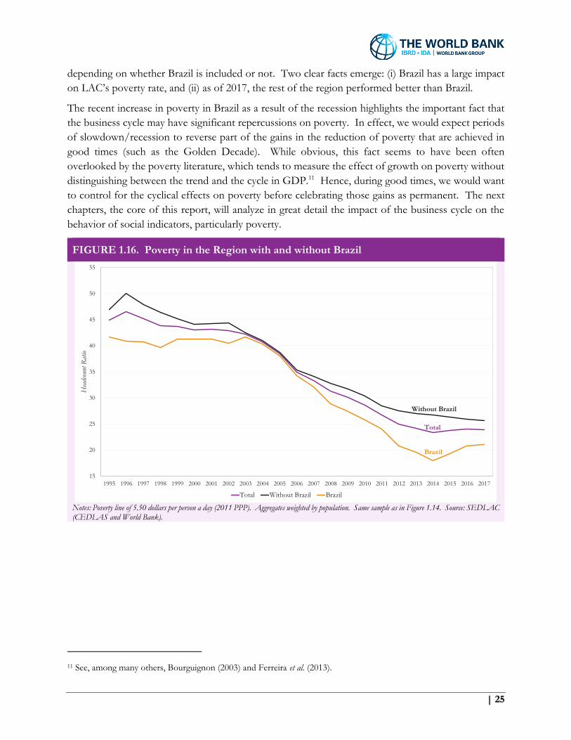
depending on whether Brazil is included or not. Two clear facts emerge: (i) Brazil has a large impact
on LAC’s poverty rate, and (ii) as of 2017, the rest of the region performed better than Brazil.
The recent increase in poverty in Brazil as a result of the recession highlights the important fact that
the business cycle may have significant repercussions on poverty. In effect, we would expect periods
of slowdown/recession to reverse part of the gains in the reduction of poverty that are achieved in
good times (such as the Golden Decade). While obvious, this fact seems to have been often
overlooked by the poverty literature, which tends to measure the effect of growth on poverty without
distinguishing between the trend and the cycle in GDP.11 Hence, during good times, we would want
to control for the cyclical effects on poverty before celebrating those gains as permanent. The next
chapters, the core of this report, will analyze in great detail the impact of the business cycle on the
behavior of social indicators, particularly poverty.
FIGURE 1.16. Poverty in the Region with and without Brazil
Notes: Poverty line of 5.50 dollars per person a day (2011 PPP). Aggregates weighted by population. Same sample as in Figure 1.14. Source: SEDLAC (CEDLAS and World Bank).
11 See, among many others, Bourguignon (2003) and Ferreira et al. (2013).
15
20
25
30
35
40
45
50
55
1995 1996 1997 1998 1999 2000 2001 2002 2003 2004 2005 2006 2007 2008 2009 2010 2011 2012 2013 2014 2015 2016 2017
Hea
dcou
nt R
atio
Total Without Brazil Brazil
Brazil
Total
Without Brazil

26 | When Dreams Meet Reality
| 27
Chapter 2
Fooled by the Cycle: Permanent versus Transitory
Improvements in Social Indicators
Introduction
When examining the evolution of social indicators over recent decades, we should always keep in
mind that any change in the underlying indicator can be decomposed into a transitory component,
typically driven by cyclical factors, and a more persistent or “permanent” component that responds
to structural factors. Taking this distinction into account is critical for policymakers since policies and
programs implemented to address the cyclical behavior of social indicators will be necessarily different
from those designed to improve structural factors. Moreover, measuring the success in the fight
against poverty using social indicators with large cyclical components could be misleading since the
analysis would be highly sensitive to the time span under study. In other words, a policymaker would
draw very different conclusions if the response of poverty were evaluated during a boom or a complete
(boom-bust) business cycle. In fact, the importance of the cyclical component in social indicators is
magnified for the case of emerging markets subject to large external shocks, such as changes in the
terms of trade, global liquidity, and world economic activity. All these shocks are cyclical in nature
and thus will tend to amplify emerging markets’ business cycles and, in turn, the transitory components
of social indicators.
This chapter is devoted to understanding the role of transitory versus structural components in the
evolution of relevant social indicators such as unemployment, monetary poverty, or unsatisfied basic
needs (UBN).12 Given that income is one of the most important drivers of economic and social
welfare, this chapter uses the business cycle (i.e., the transitory component of national income) and
long-term income changes to proxy for the transitory and permanent components of our set of social
indicators, respectively.
How Cyclical are Social Indicators?
The first key message that follows from a simple trend-cycle decomposition is that the relative
importance of transitory versus permanent changes differs greatly across social indicators. Figures
12 Given the availability of household survey data in LAC, we use the SEDLAC (CEDLAS and World Bank) UBN indicator, which comprises: (i) overcrowding (more than 4 persons per room); (ii) household living in poor location; (iii) dwelling of low-quality materials; (iv) dwelling without access to water; (v) dwelling without access to adequate restroom sanitation; (vi) children of ages 7-11 not attending school; (vii) head of household without primary school degree; and (viii) head of household without secondary school degree combined with a high dependency ratio (more than 4 household members per income earner). A person belongs to the UBN category if she is part of a household that satisfies at least one of these eight conditions.

28 | When Dreams Meet Reality
2.1, 2.2, and 2.3 illustrate this important stylized fact. Figure 2.1 traces the evolution of three widely-
used social indicators (unemployment rate, monetary poverty, and UBN) as well as the cyclical
component of real GDP per capita from 1995 to 2017 for a sample of 15 LAC countries. In terms of
cyclicality, the measures of unemployment and UBN stand at opposite extremes: while unemployment
(black line) displays a clear cyclical behavior, following closely the business cycle (red line), the UBN
series (orange line), characterized by structural factors, appears uncorrelated with the business cycle
and dominated by a permanent (trend) component.13 Monetary poverty (purple line) falls somewhere
in between, exhibiting both trend and cyclical components.
FIGURE 2.1. Monetary Poverty, UBN, Unemployment, and Cyclical Component of Real GDP per Capita in LAC
Notes: Poverty line of 5.50 dollars per person a day (2011 PPP). Averages for LAC are weighted by population. LAC aggregate based on 15 countries for which microdata are available at the national level: Argentina, Bolivia, Brazil, Chile, Colombia, Costa Rica, the Dominican Republic, El Salvador, Ecuador, Honduras, Mexico, Panama, Paraguay, Peru, and Uruguay. For sample periods, see Table E.1 in Appendix E. Due to lack of comparable data, Panama is not included in UBN. Sources: LCRCE's estimations based on SEDLAC (CEDLAS and World Bank) and WEO (October 2018).
To highlight the size and importance of these differences, Figure 2.1 normalizes to 100 to all four
measures for the year 2003 and follows the improvement of social conditions until 2014 (the period
in-between the two vertical bars). This period is typically referred to as the Golden Decade due to the
long-lasting boom in commodity prices. Depending on which social indicator we focus on, a very
different picture emerges. Both unemployment and monetary poverty had a strong response to the
13 For sure, there are, among others, two social indicators that are typically associated with structural factors: the Multidimensional Poverty Index (MPI) and the Human Capital Index (HCI), the latter recently developed as part of the 2019 World Bank Human Capital Project. Unfortunately, the MPI series are not comparable over time, which is obviously crucial for our analysis and a sufficiently large dataset is not yet available for the HCI. These measures, however, will be a highly relevant resource for future research on permanent social gains.
-140
-100
-60
-20
20
60
100
140
180
40
50
60
70
80
90
100
110
120
1995
1996
1997
1998
1999
2000
2001
2002
2003
2004
2005
2006
2007
2008
2009
2010
2011
2012
2013
2014
2015
2016
2017
Inde
x (
2003
=10
0, i
nver
ted
axis
)
Inde
x (
2003
=10
0)
Monetary Poverty Unsatisfied Basic Needs (UBN) Unemployment Real GDP per Capita (cyclical component, right axis)
Golden Decade

| 29
economic tailwinds and declined by around 40 percent for the region as a whole. The UBN indicator
also fell but at a much lower rate that was, in fact, not very different from the one before the Golden
Decade. The decline of the UBN indicator amounted to just over 20 percent during this period.
FIGURE 2.2. Contribution of Cyclical Component of Real GDP per Capita to Total Variance of Social Indicators in LAC
Notes: Poverty line of 5.50 dollars per person a day (2011 PPP). Black lines denote one-standard-error intervals. Averages and standard errors for LAC weighted by population. LAC aggregate based on 15 countries of the region for which microdata are available at the national level: Argentina, Bolivia, Brazil, Chile, Colombia, Costa Rica, Dominican Republic, El Salvador, Ecuador, Honduras, Mexico, Panama, Paraguay, Peru, and Uruguay. For sample periods, see Table E.1 in Appendix E. Due to lack of comparable data, Panama is not included in UBN. Estimations of the cyclical component based on a bivariate model. Sources: LCRCE's estimations based on SEDLAC (CEDLAS and World Bank) and WEO (October 2018).
For a casual observer standing in the year 2014, taking the large cyclical gains in unemployment and
monetary poverty at face value would lead to an over-optimistic (and, in fact, misleading) evaluation
of the permanent improvements in social conditions in the region. This biased view of reality becomes
evident once the economic cycle begins to take a turn for the worse in 2013 and a large part of these
social gains quickly start to dissipate. Had she been more careful, our casual observer could have
prevented such over-optimism (or conveying a misleading picture) by either controlling for the cyclical
component of unemployment and monetary poverty or simply basing her analysis on measures
uncorrelated with the business cycle such as the UBN indicator.
The variance decomposition presented in Figure 2.2 for a sample of 15 LAC economies and Figure
2.3 for a worldwide sample formalizes the above intuition. The height of the bars in both figures
denotes the share of the cyclical component of real GDP per capita in the total variance of each
indicator.14 Specifically, the share of the total variance explained by the business cycle is much higher
for unemployment and monetary poverty than for structural measures of social welfare such as the
14 As shown in Appendix D, the shares of the cyclical and trend components add up to 100 percent.
0.0
0.1
0.2
0.3
0.4
0.5
0.6
0.7
0.8
Unemployment Monetary Poverty UBN
Sha
re o
f C
yclica
l Com
pone
nt in
Tot
al V
aria
nce

30 | When Dreams Meet Reality
UBN or the Human Development Index (HDI).15 For LAC (Figure 2.2), the cyclical component of
real per capita output explains 74 percent of the variance of the unemployment rate.
FIGURE 2.3. Contribution of Cyclical Component of Real GDP per Capita to Total Variance of Social Indicators (World Sample)
Notes: Poverty line of 5.50 dollars per person a day (2011 PPP). Black lines denote one-standard-error intervals. Averages and standard errors for LAC are weighted by population. LAC aggregate based on 15 countries of the region for which microdata are available at the national level: Argentina, Bolivia, Brazil, Chile, Colombia, Costa Rica, Dominican Republic, El Salvador, Ecuador, Honduras, Mexico, Panama, Paraguay, Peru, and Uruguay. For periods covered and world sample, see Appendices C and E. Estimations of the cyclical component based on a bivariate model. Sources: LCRCE's estimations based on PovcalNet (September 2018), SEDLAC (CEDLAS and World Bank), WEO (October 2018), and Human Development Report Office (United Nations).
At the other extreme, the cyclical component explains only 21 percent of the variance of the UBN
indicator (and hence 79 percent is explained by the trend component). Monetary poverty falls in
between, with 43 percent of its variability due to cyclical movements in per capita output (and hence
57 percent to the trend component). The worldwide sample in Figure 2.3 presents a similar qualitative
picture with the share of the cyclical component being 48 percent for unemployment, 28 percent for
monetary poverty, and 18 percent for HDI.
These large differences in the time series behavior of different social indicators may be striking at first
sight but should hardly come as a surprise given the components of each indicator and the underlying
economic forces linking them to the evolution of aggregate income. Any Keynesian model with price
or wage rigidities would predict a strong correlation between unemployment and the business cycle.
15 A measure of UBN is not available outside our LAC sample so we use HDI as a proxy for the worldwide sample. The HDI, developed by the United Nations Development Programme, is a summary measure of average achievement in key dimensions of human development: a long and healthy life, education, and a decent standard of living. The health dimension is assessed by life expectancy at birth, the education dimension by years of schooling for adults aged 25 and over and expected years of schooling for children of school-entering age, and the standard of living dimension by national income per capita.
0.00
0.05
0.10
0.15
0.20
0.25
0.30
0.35
0.40
0.45
0.50
0.55
Unemployment Monetary Poverty HDI HDI (excl. LAC) HDI for LAC
Sha
re o
f C
yclic
al C
ompo
nent
in T
otal
Var
ianc
e

| 31
In particular, negative real or monetary shocks would lead to short-term rises in unemployment. Our
results for the U.S. economy confirm, as expected, that the share of the overall unemployment
variance explained by the cyclical component of output is around 90 percent. In sharp contrast, since
UBN comprises factors that are structural in nature and thus much less responsive to the business
cycle, we would indeed expect the trend component to play a much more important role.
As follows from the above discussion, an interesting quantitative difference arises between LAC and
the world when it comes to the share of unemployment explained by the cyclical component of output
(74 percent in LAC versus 48 percent for the world sample). Why would this be the case? Without
taking a stand into possible structural differences in labor markets between LAC and other emerging
markets and how they may respond to temporary shocks, it is worth pointing out that we can account
for most of the gap based on the higher output volatility experienced by LAC economies, typically
exposed to large external shocks. For a given and similar structural reaction of unemployment to
transitory shocks, the share of the variance explained by such shocks grows mechanically with their
volatility.16 In fact, a simple example suggests that, all else equal, the above difference (between,
roughly, 70 and 50 percent), can be explained by a difference in output cycle variances of around 60
percent (compared to an actual difference of around 50 percent).17
Unlike unemployment, the UBN indicator for LAC and the HDI for the worldwide sample are mostly
driven by changes in structural factors, such as improvements in housing, education, and health, which
are typically carried out over long periods of inclusive economic growth. Finally, changes in monetary
poverty will, by construction, depend on the evolution of income per capita and changes in its
distribution.18 How much the business cycle affects economic welfare will ultimately depend on the
existence of automatic stabilizers such as unemployment benefits and/or other policy buffers. Since
both the underlying macroeconomic volatility and the effectiveness of different social policies may
vary substantially across countries, we would expect that the relative importance of the business cycle
in explaining changes in monetary poverty would also vary significantly across countries. This is
precisely what we find in the data, leaving us with a very important corollary to our first insight: not
only is the share of the cyclical component of output different across social indicators but, in the case
of monetary poverty, it is also heterogenous across countries.
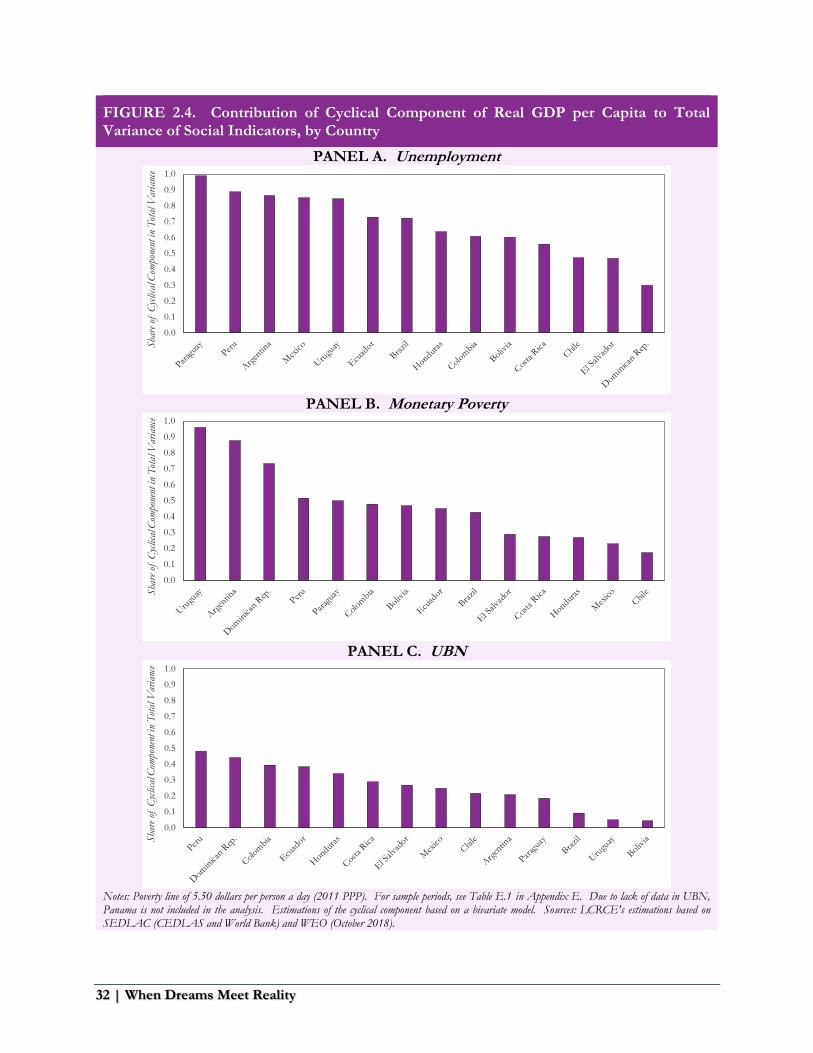
Figure 2.4 displays the same variance decomposition as in Figure 2.2 for all the countries with available
data in the region. While the shares of the cyclical component for the unemployment and UBN
indicators are quite similar across countries (particularly across larger economies), the shares in the
16 Notice that, as made clear in Appendix D, the share of the unemployment variance due to transitory output shocks depends on the size of their variance.
17 This example assumes that (i) the parameters used to calculate the output cycle share explaining the unemployment variance of two economies are all equal except for the variances of the output cycle, and (ii) parameters are calibrated such that the shares are 0.5 in one economy and 0.7 in the other. Then, the difference between output cycle variances would be around 60 percent (higher for the country with the share of 0.7). Our estimated difference in output volatility for LAC relative to advanced economies and other emerging markets is around 50 percent.
18 Chapter 3 will analyze in detail this decomposition.
32 | When Dreams Meet Reality
FIGURE 2.4. Contribution of Cyclical Component of Real GDP per Capita to Total Variance of Social Indicators, by Country
PANEL A. Unemployment
PANEL B. Monetary Poverty
PANEL C. UBN
Notes: Poverty line of 5.50 dollars per person a day (2011 PPP). For sample periods, see Table E.1 in Appendix E. Due to lack of data in UBN, Panama is not included in the analysis. Estimations of the cyclical component based on a bivariate model. Sources: LCRCE's estimations based on SEDLAC (CEDLAS and World Bank) and WEO (October 2018).
0.0
0.1
0.2
0.3
0.4
0.5
0.6
0.7
0.8
0.9
1.0
Sha
re o
f C
yclic
al C
ompo
nent
in T
otal
Var
ianc
e
0.0
0.1
0.2
0.3
0.4
0.5
0.6
0.7
0.8
0.9
1.0
Sha
re o
f C
yclic
al C
ompo
nent
in T
otal
Var
ianc
e
0.0
0.1
0.2
0.3
0.4
0.5
0.6
0.7
0.8
0.9
1.0
Sha
re o
f C
yclic
al C
ompo
nent
in T
otal
Var
ianc
e
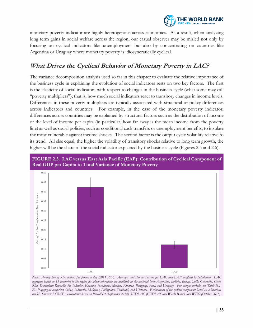
| 33
monetary poverty indicator are highly heterogenous across economies. As a result, when analyzing
long term gains in social welfare across the region, our casual observer may be misled not only by
focusing on cyclical indicators like unemployment but also by concentrating on countries like
Argentina or Uruguay where monetary poverty is idiosyncratically cyclical.
What Drives the Cyclical Behavior of Monetary Poverty in LAC?
The variance decomposition analysis used so far in this chapter to evaluate the relative importance of
the business cycle in explaining the evolution of social indicators rests on two key factors. The first
is the elasticity of social indicators with respect to changes in the business cycle (what some may call
“poverty multipliers”); that is, how much social indicators react to transitory changes in income levels.
Differences in these poverty multipliers are typically associated with structural or policy differences
across indicators and countries. For example, in the case of the monetary poverty indicator,
differences across countries may be explained by structural factors such as the distribution of income
or the level of income per capita (in particular, how far away is the mean income from the poverty
line) as well as social policies, such as conditional cash transfers or unemployment benefits, to insulate
the most vulnerable against income shocks. The second factor is the output cycle volatility relative to
its trend. All else equal, the higher the volatility of transitory shocks relative to long term growth, the
higher will be the share of the social indicator explained by the business cycle (Figures 2.5 and 2.6).
FIGURE 2.5. LAC versus East Asia Pacific (EAP): Contribution of Cyclical Component of Real GDP per Capita to Total Variance of Monetary Poverty
Notes: Poverty line of 5.50 dollars per person a day (2011 PPP). Averages and standard errors for LAC and EAP weighted by population. LAC aggregate based on 15 countries in the region for which microdata are available at the national level: Argentina, Bolivia, Brazil, Chile, Colombia, Costa Rica, Dominican Republic, El Salvador, Ecuador, Honduras, Mexico, Panama, Paraguay, Peru, and Uruguay. For sample periods, see Table E.1. EAP aggregate comprises China, Indonesia, Malaysia, Philippines, Thailand, and Vietnam. Estimations of the cyclical component based on a bivariate model. Sources: LCRCE's estimations based on PovcalNet (September 2018), SEDLAC (CEDLAS and World Bank), and WEO (October 2018).
0.00
0.05
0.10
0.15
0.20
0.25
0.30
0.35
0.40
0.45
0.50
LAC EAP
Sha
re o
f C
yclica
l Com
pone
nt in
Tot
al V
aria
nce
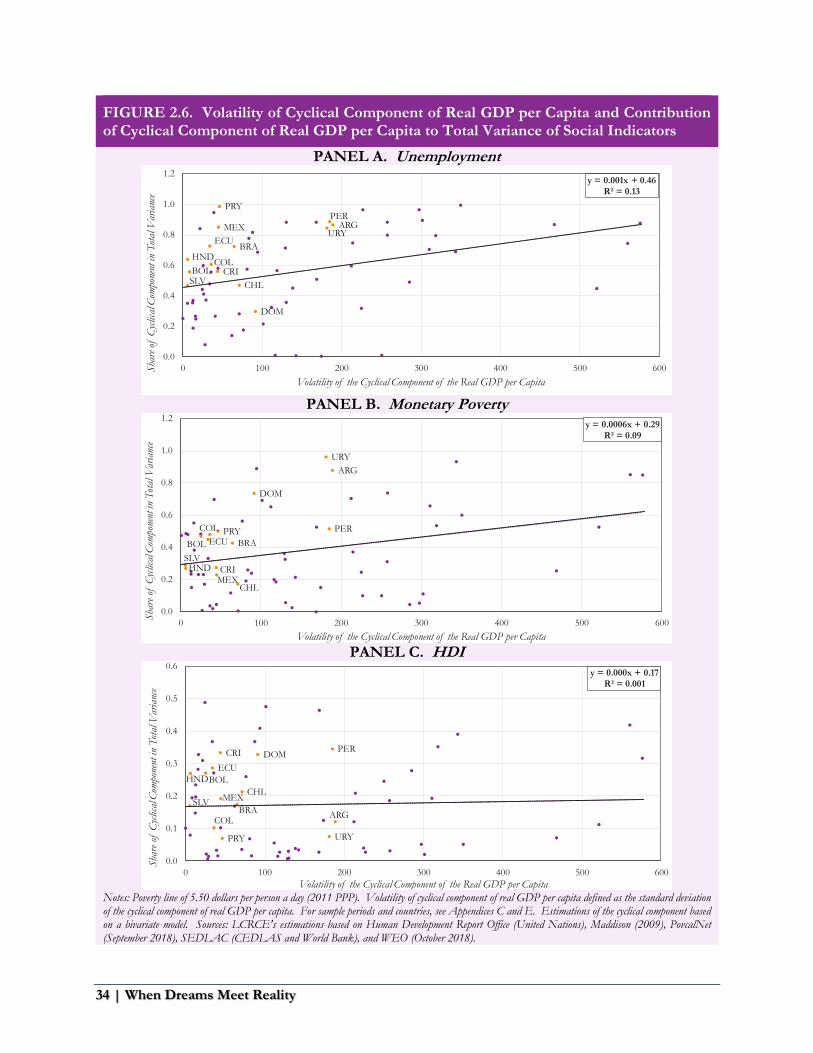
34 | When Dreams Meet Reality
FIGURE 2.6. Volatility of Cyclical Component of Real GDP per Capita and Contribution of Cyclical Component of Real GDP per Capita to Total Variance of Social Indicators
PANEL A. Unemployment
PANEL B. Monetary Poverty
PANEL C. HDI
Notes: Poverty line of 5.50 dollars per person a day (2011 PPP). Volatility of cyclical component of real GDP per capita defined as the standard deviation of the cyclical component of real GDP per capita. For sample periods and countries, see Appendices C and E. Estimations of the cyclical component based on a bivariate model. Sources: LCRCE's estimations based on Human Development Report Office (United Nations), Maddison (2009), PovcalNet (September 2018), SEDLAC (CEDLAS and World Bank), and WEO (October 2018).
ARG
BOL
BRA
CHL
COLCRI
DOM
ECU
HND
MEX
PERPRY
SLV
URY
y = 0.001x + 0.46R² = 0.13
0.0
0.2
0.4
0.6
0.8
1.0
1.2
0 100 200 300 400 500 600Sha
re o
f C
yclic
al C
ompo
nent
in T
otal
Var
ianc
e
Volatility of the Cyclical Component of the Real GDP per Capita
ARG
BOL BRA
CHL
COL
CRI
DOM
ECU
HND
MEX
PERPRY
SLV
URY
y = 0.0006x + 0.29R² = 0.09
0.0
0.2
0.4
0.6
0.8
1.0
1.2
0 100 200 300 400 500 600
Sha
re o
f C
yclic
al C
ompo
nent
in T
otal
Var
ianc
e
Volatility of the Cyclical Component of the Real GDP per Capita
ARG
BOL
BRA
CHL
COL
CRI DOM
ECUHND
MEX
PER
PRY
SLV
URY
y = 0.000x + 0.17R² = 0.001
0.0
0.1
0.2
0.3
0.4
0.5
0.6
0 100 200 300 400 500 600
Sha
re o
f C
yclic
al C
ompo
nent
in T
otal
Var
ianc
e
Volatility of the Cyclical Component of the Real GDP per Capita

| 35
Since Chapters 3 and 4 will be partly devoted to better understanding the poverty multipliers, this
section focuses on analyzing the effects of output volatility on the cyclicality of social indicators.
Output volatility becomes crucial to explain another relevant stylized fact uncovered by Figures 2.2
and 2.3: LAC displays a substantially larger cyclicality of unemployment and monetary poverty than
the rest of the world.19 Figure 2.5 helps further visualize these differences comparing the cyclicality
of monetary poverty in LAC to a sample of emerging East Asian economies. As the figure shows, the
cyclicality of monetary poverty is more than three times higher in LAC than in East Asia.
While these sizeable differences in the average cyclical shares are difficult to account for based on
structural or policy differences across regions, we know from a long-standing empirical literature that
LAC is one of the most volatile regions in the world (see, for example, Végh et al., 2018). Countries
in LAC are highly exposed to volatile external factors such as commodity prices, international liquidity,
and movements of goods and capital as well as frequent political and institutional instability. The large
volatility in the region’s business cycle could explain why LAC’s social indicators are more driven by
transitory movements in output than in other emerging markets.
Figure 2.6 depicts the relationship between output cycle volatility and the cyclicality of social indicators
using simple scatter plots. As expected, the effects of volatility measured by the slope of the fitted
line are positive for unemployment (Figure 2.6, Panel A) and monetary poverty (Figure 2.6, Panel B),
but essentially zero for HDI (Figure 2.6, Panel C). The fact that the role of output volatility seems to
be smaller in the case of monetary poverty compared to unemployment could point to the relative
effectiveness of targeted policies like unemployment benefits or conditional cash transfers that help
insulate the most vulnerable population against transitory changes in income. The structural nature
of HDI ensures a very small poverty multiplier. In other words, improvements in education and
health react very little to short-run fluctuations in the business cycle; hence, the amplitude of the cycle
plays no role in the evolution of this type of indicators.
The Perils of Random Sampling
This chapter has shown that not all social indicators are created equal, especially when it comes to
their degree of cyclicality. These stylized facts lead to a powerful policy warning: given the prevalence
of temporary gains and losses in the measures of social welfare, a policymaker focusing on an indicator
with a relatively short time span of available data could be highly misled in her efforts to evaluate
permanent improvements in social conditions.
To illustrate this warning, consider a simple example with two countries and two different indicators:
monetary poverty, which will be quite cyclical, and UBN, which will be rather unresponsive to changes
in the business cycle. Further, to factor in the volatility dimension, we purposefully pick two large
economies in our region with very different shares of cyclicality in monetary poverty, Argentina and
Chile (Figure 2.7, Panels A and B, respectively).
19 Higher output volatility in the region could also affect the shares of cyclicality in structural measures like HDI but, since the elasticities in these indicators are close to zero, overall differences across regions would remain very small.

36 | When Dreams Meet Reality
FIGURE 2.7. Argentina versus Chile: Monetary Poverty and UBN
PANEL A. Argentina PANEL B. Chile
PANEL C.
Monetary Poverty: 10-Year Moving Change
PANEL D. UBN: 10-Year Moving Change
PANEL E.
Distribution of 10-Year Moving Change of Monetary Poverty
PANEL F. Distribution of 10-Year Moving
Change of UBN
Notes: Poverty line of 5.50 dollars per person a day (2011 PPP). Sources: LCRCE's estimations based on SEDLAC (CEDLAS and World Bank) and WEO (October 2018).
0
5
10
15
20
25
0
5
10
15
20
25
30
35
40
45
50
1991
1992
1993
1994
1995
1996
1997
1998
1999
2000
2001
2002
2003
2004
2005
2006
2007
2008
2009
2010
2011
2012
2013
2014
2015
2016
2017
Tho
usan
ds o
f D
olla
rs, 2011 P
PP
As
perc
enta
ge o
f po
pula
tion
Monetary Poverty UBN Real GDP per capita (right axis)
0
5
10
15
20
25
0
10
20
30
40
50
60
1990
1991
1992
1993
1994
1995
1996
1997
1998
1999
2000
2001
2002
2003
2004
2005
2006
2007
2008
2009
2010
2011
2012
2013
2014
2015
Tho
usan
ds o
fD
olla
rs, 2011 P
PP
As
perc
enta
ge o
f po
pula
tion
Monetary Poverty UBN Real GDP per capita (right axis)
-40
-30
-20
-10
0
10
20
30
40
2001
2002
2003
2004
2005
2006
2007
2008
2009
2010
2011
2012
2013
2014
201510-Y
ear
Mov
ing
Cha
nge
(in
perc
enta
ge p
oint
s)
Argentina Chile
-40
-30
-20
-10
0
10
20
30
40
2001
2002
2003
2004
2005
2006
2007
2008
2009
2010
2011
2012
2013
2014
201510-Y
ear
Mov
ing
Cha
nge
(in
perc
enta
ge p
oint
s)
Argentina Chile
0.00
0.05
0.10
0.15
0.20
0.25
0.30
0.35
0.40
0.45
-2.9
-2.6
-2.3
-1.9
-1.6
-1.3
-0.9
-0.6
-0.3
0.1
0.4
0.8
1.1
1.4
1.8
2.1
2.4
2.8
3.1
3.4
3.8
Den
sity
Standarized 10-Year Moving Change in Monetary Poverty
Argentina Chile
0.00
0.05
0.10
0.15
0.20
0.25
0.30
0.35
0.40
0.45
-3.2
-2.8
-2.5
-2.1
-1.7
-1.4
-1.0
-0.7
-0.3
0.1
0.4
0.8
1.2
1.5
1.9
2.2
2.6
3.0
3.3
3.7
4.1
4.4
4.8
Den
sity
Standarized 10-Year Moving Change in UBN
Argentina Chile

| 37
Panels A and B in Figure 2.7 display the evolution of real GDP per capita, monetary poverty, and
UBN for Argentina and Chile, respectively. We can already see large differences in both the business
cycle and monetary poverty across the two economies. Argentina endures large swings in real GDP
that are matched by relatively large responses in the monetary poverty indicator. In sharp contrast,
the amplitude of Chile’s business cycle is very small and both real GDP and monetary poverty seem
to be clearly driven by a trend. Interestingly, in both cases, the UBN indicator is driven by a trend
regardless of the underlying business cycle.
Suppose now that our policymaker is trying to evaluate the long-run improvement of social conditions
but is restricted to one decade of data. Figure 2.7, Panels C and D show the 10-year moving difference
in the monetary poverty and UBN indicators. These figures give us a clear sense of the potential
biases in perception across different samples. In Argentina, a policymaker evaluating social welfare
gains using the monetary poverty indicator in 2002 would reach the opposite conclusions than one
evaluating the situation in 2012. These large differences make it almost impossible to understand the
long-term evolution of social conditions in the country. On the other hand, a policymaker using the
same indicator in Chile would be much less exposed to sample-dependent variation in her conclusions.
In other words, since the monetary poverty indicator in Chile is dominated by the trend component,
we can approximate the long-run gains in the underlying indicator with relative short-time samples.
Notably, a policymaker using the UBN indicator would not fall into the trap of sample dependent
conclusions regardless of the country under study.
Finally, Figure 2.7, Panels E and F translate the previous results into a density function for the 10-year
moving differences in monetary poverty and UBN, respectively. The differences in the variance of
the distributions for monetary poverty in Figure 2.7, Panel E tell us that a policymaker from Argentina
is more exposed to relatively large errors than one from Chile. The fat tails in the distribution for
Argentina also indicate that those errors could be extremely large. Using instead UBN as an indicator
not only lowers the chances of sample-dependent errors but also eliminates the differences across
countries, as shown in Figure 2.7, Panel F.
Are Structural Indicators such as HDI Structural Enough?
This chapter has emphasized the potential bias implicit in cyclical social indicators when trying to
evaluate permanent improvements in social conditions. A simple solution would be to extract the
trend component of each indicator and use that trend in the evaluation of long-run gains in poverty
reduction. The problem with this approach is the risk of sample-dependent bias explained above due
to the short sample of available data. An alternative solution comes from the type of indicator used.
Throughout the chapter, we have seen that social indicators based on structural factors such as UBN
or HDI are much less influenced by transitory shocks. The large trend component in these indicators
implies that we can better proxy long-run improvements in social conditions with relatively short
periods of available data.
Having said that, indicators such as HDI are also subject to some degree of cyclicality because of the
composition of the index. Figure 2.8, Panel A decomposes the HDI indicator in its three components
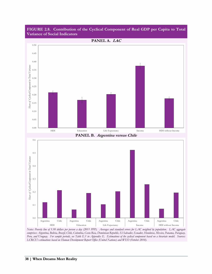
38 | When Dreams Meet Reality
FIGURE 2.8. Contribution of the Cyclical Component of Real GDP per Capita to Total Variance of Social Indicators
PANEL A. LAC
PANEL B. Argentina versus Chile
Notes: Poverty line of 5.50 dollars per person a day (2011 PPP). Averages and standard errors for LAC weighted by population. LAC aggregate comprises: Argentina, Bolivia, Brazil, Chile, Colombia, Costa Rica, Dominican Republic, El Salvador, Ecuador, Honduras, Mexico, Panama, Paraguay, Peru, and Uruguay. For sample periods, see Table E.1 in Appendix E. Estimations of the cyclical component based on a bivariate model. Sources: LCRCE's estimations based on Human Development Report Office (United Nations) and WEO (October 2018).
0.00
0.05
0.10
0.15
0.20
0.25
0.30
0.35
0.40
0.45
0.50
HDI Education Life Expectancy Income HDI without Income
Sha
re o
f C
yclic
al C
ompo
nent
in T
otal
Var
ianc
e
0.0
0.1
0.2
0.3
0.4
0.5
0.6
Argentina Chile Argentina Chile Argentina Chile Argentina Chile Argentina Chile
HDI Education Life Expectancy Income HDI without Income
Sha
re o
f C
yclic
al C
ompo
nent
in T
otal
Var
ianc
e
| 39
and shows their share of cyclicality for LAC. While structural components such as education and life
expectancy are quite unrelated to the business cycle, the measure of income included in the index is,
as expected, much more influenced by the business cycle. Again, including such cyclical components
in the construction of structural measures like HDI would affect some countries more than others
depending on the underlying volatility of the business cycle, as shown in Figure 2.8, Panel B where
the cyclicality of the income component is twice as large in Argentina than in Chile.
What Have We Learned?
This chapter has uncovered a set of important stylized facts regarding the cyclical nature of social
indicators. First, not all social indicators are created equal. Indicators such as unemployment or
monetary poverty tend to comove with the business cycle. Second, structural indicators such as UBN
or HDI mainly co-move with long-run economic growth. Thirdly, contrary to our findings in
unemployment, UBN, and HDI, the degree of cyclicality in monetary poverty is highly heterogenous
across countries.
These differences may be due to variations in the amplitude of business cycles across countries or the
effectiveness of anti-poverty measures designed to insulate the most vulnerable individuals from
transitory shocks in the economy. Finally, both unemployment and monetary poverty tend to be more
cyclical in LAC than in other emerging markets. Part of this difference may be due to the higher
volatility of output endured by our region compared to other emerging markets.
These stylized facts are particularly relevant for policymakers trying to evaluate the long-term changes
in social conditions using relatively short time series. Our results alert about the possibility of sample-
dependent conclusions when using highly cyclical social indicators. This risk is higher for countries
exposed to large income cycles. To avoid these biases, policymakers should rely on structural
indicators dominated by trend components to evaluate long-term improvements in social welfare.

40 | When Dreams Meet Reality
| 41
Chapter 3
Decomposition of Fall in Monetary Poverty during
the Golden Decade in LAC
Introduction
The previous chapter showed that while some social indicators (such as the unemployment rate) are
tightly linked to the business cycle and will thus fluctuate considerably in the short run, others (such
as UBN and HDI) follow essentially the long-run trend in GDP per capita, and hence bear almost no
relation to the business cycle. Interestingly, in the case of the LAC region, monetary poverty lies
somewhere in between the two extremes just mentioned, with large heterogeneity across countries.
In particular, whether monetary poverty behaves more like the unemployment rate (i.e., affected
mainly by the business cycle) or UBN and HDI (i.e., determined essentially by the long-run trend in
GDP per capita) crucially depends on the volatility of the business cycle. In high volatility countries
(such as Argentina), changes in monetary poverty are much more closely related to the business cycle
than in low volatility countries (such as Chile).
Given this insight, a natural question arises: how much of the fall in monetary poverty during the
Golden Decade was permanent and how much was transitory? As argued in Chapter 1, the LAC
region made tremendous progress in terms of reducing monetary poverty during this period, with the
headcount ratio for the 5.50-dollar poverty line falling by almost 20 percentage points (from 42.2
percent in 2003 to 23.4 in 2014). Needless to say, the relative importance of permanent versus
temporary reductions in poverty has critical implications for (i) assessing the “true” magnitude of the
fall in poverty and how lasting it may be, and (ii) the public policies that may be put in place to
address/influence permanent versus temporary falls in poverty (which in turn are likely to differ across
countries depending on output volatility). To decompose the fall in monetary poverty between
permanent and transitory components, we will follow a very helpful methodology proposed in a
seminal paper by Datt and Ravallion (1992).
The Datt and Ravallion Decomposition
Using microdata from household surveys, Datt and Ravallion (1992) decompose the change in poverty
between two points in time into (i) a “growth component” and (ii) a “redistribution component.” The
growth component is identified as the change in monetary poverty between two years that would have
occurred if the income of each household member had changed in the same proportion as the national
mean income, keeping constant the shape of the income distribution (measured by the Lorenz curve).
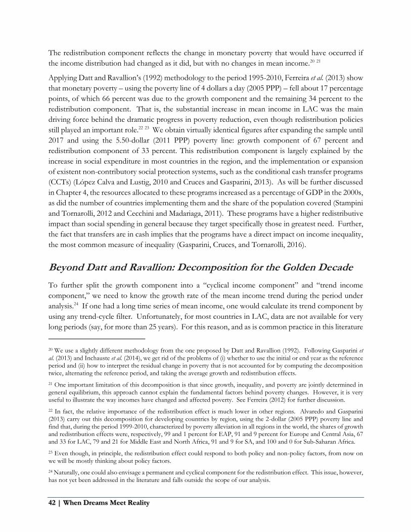
42 | When Dreams Meet Reality
The redistribution component reflects the change in monetary poverty that would have occurred if
the income distribution had changed as it did, but with no changes in mean income.20 21
Applying Datt and Ravallion’s (1992) methodology to the period 1995-2010, Ferreira et al. (2013) show
that monetary poverty – using the poverty line of 4 dollars a day (2005 PPP) – fell about 17 percentage
points, of which 66 percent was due to the growth component and the remaining 34 percent to the
redistribution component. That is, the substantial increase in mean income in LAC was the main
driving force behind the dramatic progress in poverty reduction, even though redistribution policies
still played an important role.22 23 We obtain virtually identical figures after expanding the sample until
2017 and using the 5.50-dollar (2011 PPP) poverty line: growth component of 67 percent and
redistribution component of 33 percent. This redistribution component is largely explained by the
increase in social expenditure in most countries in the region, and the implementation or expansion
of existent non-contributory social protection systems, such as the conditional cash transfer programs
(CCTs) (López Calva and Lustig, 2010 and Cruces and Gasparini, 2013). As will be further discussed
in Chapter 4, the resources allocated to these programs increased as a percentage of GDP in the 2000s,
as did the number of countries implementing them and the share of the population covered (Stampini
and Tornarolli, 2012 and Cecchini and Madariaga, 2011). These programs have a higher redistributive
impact than social spending in general because they target specifically those in greatest need. Further,
the fact that transfers are in cash implies that the programs have a direct impact on income inequality,
the most common measure of inequality (Gasparini, Cruces, and Tornarolli, 2016).
Beyond Datt and Ravallion: Decomposition for the Golden Decade
To further split the growth component into a “cyclical income component” and “trend income
component,” we need to know the growth rate of the mean income trend during the period under
analysis.24 If one had a long time series of mean income, one would calculate its trend component by
using any trend-cycle filter. Unfortunately, for most countries in LAC, data are not available for very
long periods (say, for more than 25 years). For this reason, and as is common practice in this literature
20 We use a slightly different methodology from the one proposed by Datt and Ravallion (1992). Following Gasparini et al. (2013) and Inchauste et al. (2014), we get rid of the problems of (i) whether to use the initial or end year as the reference period and (ii) how to interpret the residual change in poverty that is not accounted for by computing the decomposition twice, alternating the reference period, and taking the average growth and redistribution effects.
21 One important limitation of this decomposition is that since growth, inequality, and poverty are jointly determined in general equilibrium, this approach cannot explain the fundamental factors behind poverty changes. However, it is very useful to illustrate the way incomes have changed and affected poverty. See Ferreira (2012) for further discussion.
22 In fact, the relative importance of the redistribution effect is much lower in other regions. Alvaredo and Gasparini (2013) carry out this decomposition for developing countries by region, using the 2-dollar (2005 PPP) poverty line and find that, during the period 1999-2010, characterized by poverty alleviation in all regions in the world, the shares of growth and redistribution effects were, respectively, 99 and 1 percent for EAP, 91 and 9 percent for Europe and Central Asia, 67 and 33 for LAC, 79 and 21 for Middle East and North Africa, 91 and 9 for SA, and 100 and 0 for Sub-Saharan Africa.
23 Even though, in principle, the redistribution effect could respond to both policy and non-policy factors, from now on we will be mostly thinking about policy factors.
24 Naturally, one could also envisage a permanent and cyclical component for the redistribution effect. This issue, however, has not yet been addressed in the literature and falls outside the scope of our analysis.
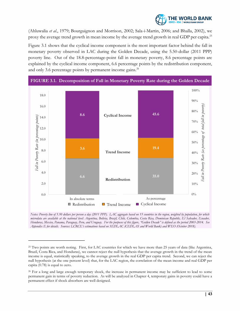
| 43
(Ahluwalia et al., 1979; Bourguignon and Morrison, 2002; Sala-i-Martin, 2006; and Bhalla, 2002), we
proxy the average trend growth in mean income by the average trend growth in real GDP per capita.25
Figure 3.1 shows that the cyclical income component is the most important factor behind the fall in
monetary poverty observed in LAC during the Golden Decade, using the 5.50-dollar (2011 PPP)
poverty line. Out of the 18.8-percentage-point fall in monetary poverty, 8.6 percentage points are
explained by the cyclical income component, 6.6 percentage points by the redistribution component,
and only 3.6 percentage points by permanent income gains.26
FIGURE 3.1. Decomposition of Fall in Monetary Poverty Rate during the Golden Decade
Notes: Poverty line of 5.50 dollars per person a day (2011 PPP). LAC aggregate based on 15 countries in the region, weighted by population, for which microdata are available at the national level: Argentina, Bolivia, Brazil, Chile, Colombia, Costa Rica, Dominican Republic, El Salvador, Ecuador, Honduras, Mexico, Panama, Paraguay, Peru, and Uruguay. For the purposes of this figure, “Golden Decade” is defined as the period 2003-2014. See Appendix E for details. Sources: LCRCE’s estimations based on SEDLAC (CEDLAS and World Bank) and WEO (October 2018).
25 Two points are worth noting. First, for LAC countries for which we have more than 25 years of data (like Argentina, Brazil, Costa Rica, and Honduras), we cannot reject the null hypothesis that the average growth in the trend of the mean income is equal, statistically speaking, to the average growth in the real GDP per capita trend. Second, we can reject the null hypothesis (at the one percent level) that, for the LAC region, the correlation of the mean income and real GDP per capita (0.78) is equal to zero.
26 For a long and large enough temporary shock, the increase in permanent income may be sufficient to lead to some permanent gain in terms of poverty reduction. As will be analyzed in Chapter 4, temporary gains in poverty could have a permanent effect if shock absorbers are well designed.
6.6
3.6
8.6
0.0
2.0
4.0
6.0
8.0
10.0
12.0
14.0
16.0
18.0
In absolute terms
Fal
l in
Pov
erty
Rat
e (in
perc
enta
ge p
oint
s)
35.0
19.4
45.6
As percentage
0%
10%
20%
30%
40%
50%
60%
70%
80%
90%
100%
Fal
l in
Pov
erty
Rat
e (a
s pe
rcen
tage
of
tota
l fal
l in
pove
rty)
Cyclical Income
Trend Income
Redistribution
Trend Income Cyclical IncomeRedistribution
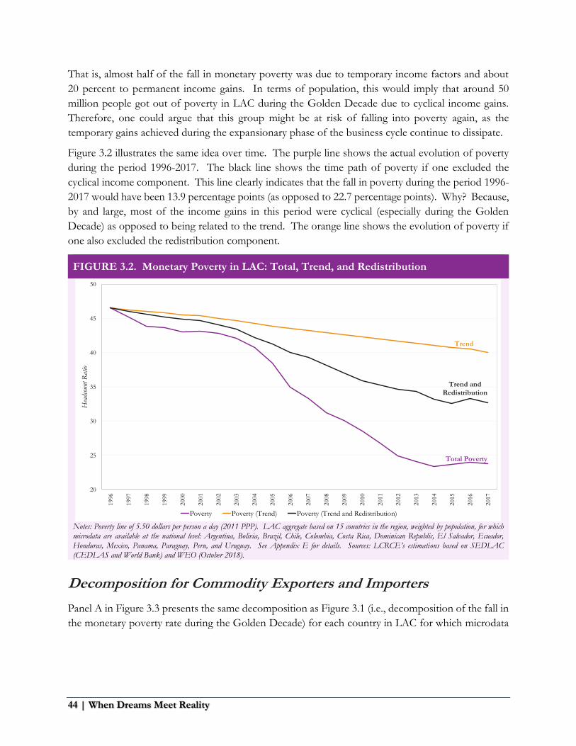
44 | When Dreams Meet Reality
That is, almost half of the fall in monetary poverty was due to temporary income factors and about
20 percent to permanent income gains. In terms of population, this would imply that around 50
million people got out of poverty in LAC during the Golden Decade due to cyclical income gains.
Therefore, one could argue that this group might be at risk of falling into poverty again, as the
temporary gains achieved during the expansionary phase of the business cycle continue to dissipate.
Figure 3.2 illustrates the same idea over time. The purple line shows the actual evolution of poverty
during the period 1996-2017. The black line shows the time path of poverty if one excluded the
cyclical income component. This line clearly indicates that the fall in poverty during the period 1996-
2017 would have been 13.9 percentage points (as opposed to 22.7 percentage points). Why? Because,
by and large, most of the income gains in this period were cyclical (especially during the Golden
Decade) as opposed to being related to the trend. The orange line shows the evolution of poverty if
one also excluded the redistribution component.
FIGURE 3.2. Monetary Poverty in LAC: Total, Trend, and Redistribution
Notes: Poverty line of 5.50 dollars per person a day (2011 PPP). LAC aggregate based on 15 countries in the region, weighted by population, for which microdata are available at the national level: Argentina, Bolivia, Brazil, Chile, Colombia, Costa Rica, Dominican Republic, El Salvador, Ecuador, Honduras, Mexico, Panama, Paraguay, Peru, and Uruguay. See Appendix E for details. Sources: LCRCE’s estimations based on SEDLAC (CEDLAS and World Bank) and WEO (October 2018).
Decomposition for Commodity Exporters and Importers
Panel A in Figure 3.3 presents the same decomposition as Figure 3.1 (i.e., decomposition of the fall in
the monetary poverty rate during the Golden Decade) for each country in LAC for which microdata
20
25
30
35
40
45
50
1996
1997
1998
1999
2000
2001
2002
2003
2004
2005
2006
2007
2008
2009
2010
2011
2012
2013
2014
2015
2016
2017
Hea
dcou
nt R
atio
Poverty Poverty (Trend) Poverty (Trend and Redistribution)
Total Poverty
Trend and Redistribution
Trend
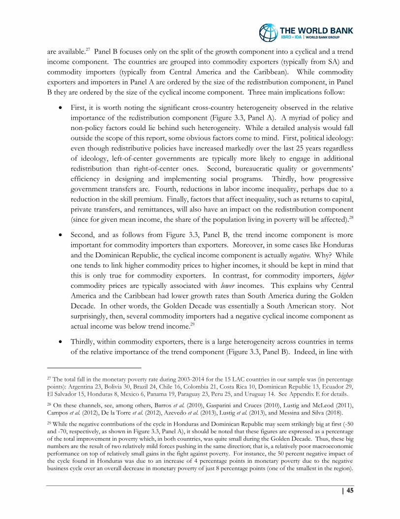
| 45
are available.27 Panel B focuses only on the split of the growth component into a cyclical and a trend
income component. The countries are grouped into commodity exporters (typically from SA) and
commodity importers (typically from Central America and the Caribbean). While commodity
exporters and importers in Panel A are ordered by the size of the redistribution component, in Panel
B they are ordered by the size of the cyclical income component. Three main implications follow:
• First, it is worth noting the significant cross-country heterogeneity observed in the relative
importance of the redistribution component (Figure 3.3, Panel A). A myriad of policy and
non-policy factors could lie behind such heterogeneity. While a detailed analysis would fall
outside the scope of this report, some obvious factors come to mind. First, political ideology:
even though redistributive policies have increased markedly over the last 25 years regardless
of ideology, left-of-center governments are typically more likely to engage in additional
redistribution than right-of-center ones. Second, bureaucratic quality or governments’
efficiency in designing and implementing social programs. Thirdly, how progressive
government transfers are. Fourth, reductions in labor income inequality, perhaps due to a
reduction in the skill premium. Finally, factors that affect inequality, such as returns to capital,
private transfers, and remittances, will also have an impact on the redistribution component
(since for given mean income, the share of the population living in poverty will be affected).28
• Second, and as follows from Figure 3.3, Panel B, the trend income component is more
important for commodity importers than exporters. Moreover, in some cases like Honduras
and the Dominican Republic, the cyclical income component is actually negative. Why? While
one tends to link higher commodity prices to higher incomes, it should be kept in mind that
this is only true for commodity exporters. In contrast, for commodity importers, higher
commodity prices are typically associated with lower incomes. This explains why Central
America and the Caribbean had lower growth rates than South America during the Golden
Decade. In other words, the Golden Decade was essentially a South American story. Not
surprisingly, then, several commodity importers had a negative cyclical income component as
actual income was below trend income.29
• Thirdly, within commodity exporters, there is a large heterogeneity across countries in terms
of the relative importance of the trend component (Figure 3.3, Panel B). Indeed, in line with
27 The total fall in the monetary poverty rate during 2003-2014 for the 15 LAC countries in our sample was (in percentage points): Argentina 23, Bolivia 30, Brazil 24, Chile 16, Colombia 21, Costa Rica 10, Dominican Republic 13, Ecuador 29, El Salvador 15, Honduras 8, Mexico 6, Panama 19, Paraguay 23, Peru 25, and Uruguay 14. See Appendix E for details.
28 On these channels, see, among others, Barros et al. (2010), Gasparini and Cruces (2010), Lustig and McLeod (2011), Campos et al. (2012), De la Torre et al. (2012), Azevedo et al. (2013), Lustig et al. (2013), and Messina and Silva (2018).
29 While the negative contributions of the cycle in Honduras and Dominican Republic may seem strikingly big at first (-50 and -70, respectively, as shown in Figure 3.3, Panel A), it should be noted that these figures are expressed as a percentage of the total improvement in poverty which, in both countries, was quite small during the Golden Decade. Thus, these big numbers are the result of two relatively mild forces pushing in the same direction; that is, a relatively poor macroeconomic performance on top of relatively small gains in the fight against poverty. For instance, the 50 percent negative impact of the cycle found in Honduras was due to an increase of 4 percentage points in monetary poverty due to the negative business cycle over an overall decrease in monetary poverty of just 8 percentage points (one of the smallest in the region).
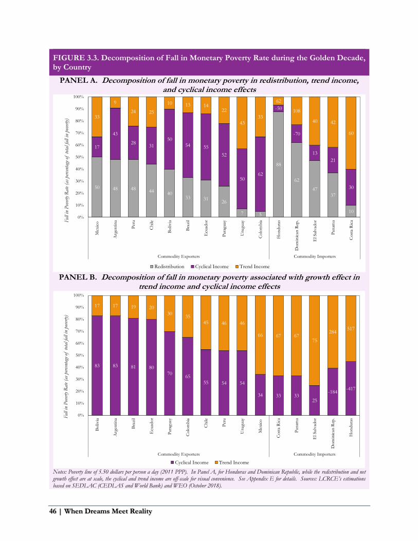
46 | When Dreams Meet Reality
FIGURE 3.3. Decomposition of Fall in Monetary Poverty Rate during the Golden Decade, by Country
PANEL A. Decomposition of fall in monetary poverty in redistribution, trend income, and cyclical income effects
PANEL B. Decomposition of fall in monetary poverty associated with growth effect in
trend income and cyclical income effects
Notes: Poverty line of 5.50 dollars per person a day (2011 PPP). In Panel A, for Honduras and Dominican Republic, while the redistribution and net growth effect are at scale, the cyclical and trend income are off-scale for visual convenience. See Appendix E for details. Sources: LCRCE’s estimations based on SEDLAC (CEDLAS and World Bank) and WEO (October 2018).
50 48 48 44 4033 31
26
7 5
88
62
4737
10
17
43
2831
5054 55
52
5062
-50
-70
13
21
30
33
9
24 25
10 13 1422
4333
62
108
40 42
60
0%
10%
20%
30%
40%
50%
60%
70%
80%
90%
100%M
exic
o
Arg
enti
na
Per
u
Chile
Bo
livia
Bra
zil
Ecu
ado
r
Par
aguay
Uru
guay
Colo
mb
ia
Ho
nd
ura
s
Do
min
ican
Rep
.
El Sal
vad
or
Pan
ama
Cost
a R
ica
Commodity Exporters Commodity Importers
Fal
l in
Pov
erty
Rat
e (a
s pe
rcen
tage
of
tota
l fal
l in
pove
rty)
Redistribution Cyclical Income Trend Income
83 83 81 8070
6555 54 54
34 33 3325
-184-417
17 17 19 2030
3545 46 46
66 67 6775
284517
0%
10%
20%
30%
40%
50%
60%
70%
80%
90%
100%
Bo
livia
Arg
enti
na
Bra
zil
Ecu
ado
r
Par
aguay
Colo
mb
ia
Chile
Per
u
Uru
guay
Mex
ico
Cost
a R
ica
Pan
ama
El Sal
vad
or
Do
min
ican
Rep
.
Ho
nd
ura
s
Commodity Exporters Commodity Importers
Fal
l in
Pov
erty
Rat
e (a
s pe
rcen
tage
of
tota
l fal
l in
pove
rty)
Cyclical Income Trend Income
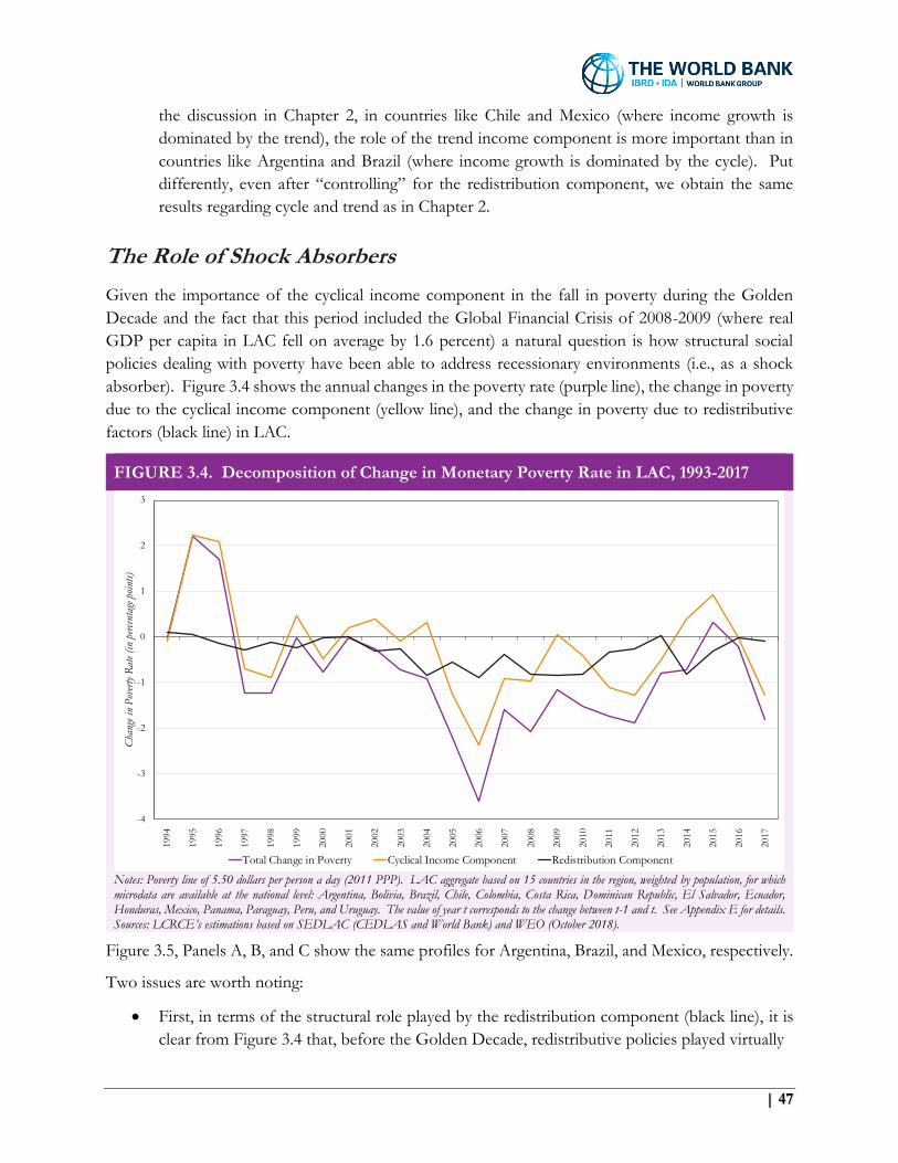
| 47
the discussion in Chapter 2, in countries like Chile and Mexico (where income growth is
dominated by the trend), the role of the trend income component is more important than in
countries like Argentina and Brazil (where income growth is dominated by the cycle). Put
differently, even after “controlling” for the redistribution component, we obtain the same
results regarding cycle and trend as in Chapter 2.
The Role of Shock Absorbers
Given the importance of the cyclical income component in the fall in poverty during the Golden
Decade and the fact that this period included the Global Financial Crisis of 2008-2009 (where real
GDP per capita in LAC fell on average by 1.6 percent) a natural question is how structural social
policies dealing with poverty have been able to address recessionary environments (i.e., as a shock
absorber). Figure 3.4 shows the annual changes in the poverty rate (purple line), the change in poverty
due to the cyclical income component (yellow line), and the change in poverty due to redistributive
factors (black line) in LAC.
FIGURE 3.4. Decomposition of Change in Monetary Poverty Rate in LAC, 1993-2017
Notes: Poverty line of 5.50 dollars per person a day (2011 PPP). LAC aggregate based on 15 countries in the region, weighted by population, for which microdata are available at the national level: Argentina, Bolivia, Brazil, Chile, Colombia, Costa Rica, Dominican Republic, El Salvador, Ecuador, Honduras, Mexico, Panama, Paraguay, Peru, and Uruguay. The value of year t corresponds to the change between t-1 and t. See Appendix E for details. Sources: LCRCE’s estimations based on SEDLAC (CEDLAS and World Bank) and WEO (October 2018).
Figure 3.5, Panels A, B, and C show the same profiles for Argentina, Brazil, and Mexico, respectively.
Two issues are worth noting:
• First, in terms of the structural role played by the redistribution component (black line), it is
clear from Figure 3.4 that, before the Golden Decade, redistributive policies played virtually
-4
-3
-2
-1
0
1
2
3
1994
1995
1996
1997
1998
1999
2000
2001
2002
2003
2004
2005
2006
2007
2008
2009
2010
2011
2012
2013
2014
2015
2016
2017
Cha
nge
in P
over
ty R
ate
(in
perc
enta
ge p
oint
s)
Total Change in Poverty Cyclical Income Component Redistribution Component
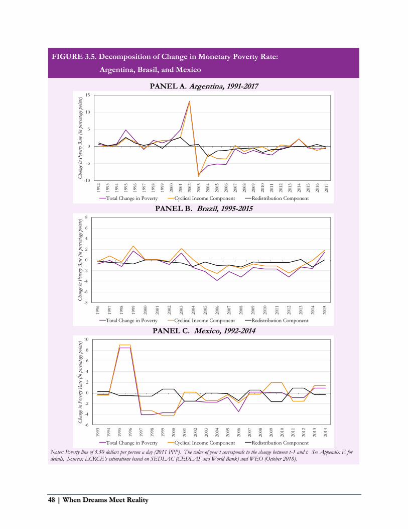
48 | When Dreams Meet Reality
FIGURE 3.5. Decomposition of Change in Monetary Poverty Rate:
Argentina, Brasil, and Mexico
PANEL A. Argentina, 1991-2017
PANEL B. Brazil, 1995-2015
PANEL C. Mexico, 1992-2014
Notes: Poverty line of 5.50 dollars per person a day (2011 PPP). The value of year t corresponds to the change between t-1 and t. See Appendix E for details. Sources: LCRCE’s estimations based on SEDLAC (CEDLAS and World Bank) and WEO (October 2018).
-10
-5
0
5
10
151992
1993
1994
1995
1996
1997
1998
1999
2000
2001
2002
2003
2004
2005
2006
2007
2008
2009
2010
2011
2012
2013
2014
2015
2016
2017
Cha
nge
in P
over
ty R
ate
(in
perc
enta
ge p
oint
s)
Total Change in Poverty Cyclical Income Component Redistribution Component
-8
-6
-4
-2
0
2
4
6
8
1996
1997
1998
1999
2000
2001
2002
2003
2004
2005
2006
2007
2008
2009
2010
2011
2012
2013
2014
2015
Cha
nge
in P
over
ty R
ate
(in
perc
enta
ge p
oint
s)
Total Change in Poverty Cyclical Income Component Redistribution Component
-6
-4
-2
0
2
4
6
8
10
1993
1994
1995
1996
1997
1998
1999
2000
2001
2002
2003
2004
2005
2006
2007
2008
2009
2010
2011
2012
2013
2014
Cha
nge
in P
over
ty R
ate
(in
perc
enta
ge p
oint
s)
Total Change in Poverty Cyclical Income Component Redistribution Component
| 49
no role. Around 2003, however, redistributive policies took great importance and
systematically reduced poverty throughout the Golden Decade and beyond.30 In fact, during
the period 2004-2010, the redistribution component caused poverty to fall by about 1
percentage point per year, a remarkable feat. Argentina and Brazil are good examples of the
important role of redistributive policies during the Golden Decade (Figure 3.5, panels A and
B, respectively).
• Second, the role of redistributive policies also changed in a very important dimension; that is,
in dealing with a recessionary environment (i.e., acting as a shock absorber). Before the
Golden Decade – and in line with its limited structural role as well – the redistribution
component played no role in helping the economy cope with changes in poverty caused by
the business cycle. During the Tequila Crisis (1995-1996), for example, poverty in LAC
increased by 2.2 percentage points, mainly driven by the cyclical components in Argentina and
Mexico (Figure 3.5, Panels A and C) and redistributive policies did not help at all (Figure 3.4).
In other words, there were no countercyclical social safety nets in place to protect the most
vulnerable in bad times, except for a few LAC countries. Their role changed during the
Golden Decade and afterwards. For example, during the Global Financial Crisis of 2008-
2009, the effect of the cyclical income component (around zero in 2009) would have implied
a stop in the fall in poverty observed since the early 2000s. Poverty, however, continued to
fall thanks to redistributive policies (Figure 3.4). This point can also be seen very clearly in
the case of Mexico in 2009-2010 (Figure 3.5, Panel C) where we can see that cyclical
considerations would have called for an increase in poverty but this was exactly offset by
redistributive policies, so that poverty did not change at all.
As the next chapter will show, the nature of these shock absorbers was not the same as in
developed countries (where they operate mainly through unemployment insurance), but rather by
an unintended consequence of how the conditional cash transfers work over the business cycle.
The number of beneficiaries tends to increase in bad times but not fall in good times, which helps
poor people in bad times but imparts a downward rigidity in these types of programs that make
them unsuitable to handle cyclical shocks and, in turn, could tend to perpetuate some inherent
problems the LAC region faces in terms of reducing informality.
30 CCTs played a major role during this period. See, among others, López Calva and Lustig (2010), Stampini and Tornarolli (2012), and Cruces and Gasparini (2013).

50 | When Dreams Meet Reality
| 51
Chapter 4
Social Transfers in LAC: In Search of Shock
Absorbers
Introduction
As discussed in Chapter 3 – and in the poverty literature in general – redistributive policies have
become more important in reducing poverty in LAC since the onset of the Golden Decade (although,
on average, the contribution of redistributive policies was smaller than the cyclical income boost). In
practice, moreover, redistributive policies have also acted as shock absorbers and prevented, for
example, a reversal in social gains during short recessionary periods such as the Global Financial Crisis
(2008-2009). What were the main factors behind the successful expansion of redistributive policies,
which even proved resilient in response to some harsh economic conditions? As suggested below,
the reasons are two-fold: (i) the incremental implementation of social programs throughout the region
in a much greater scale than before, and (ii) higher social spending during recessions (i.e., shock
absorbers). Unfortunately, the role of redistributive policies as shock absorbers has been, more often
than not, a welcome but unintended consequence of programs that had been originally designed to
address long-run (structural) poverty conditions rather than to smooth out the business cycle. An
important policy lesson is thus that the region should develop, in addition to existing structural
programs, social safety net tools that can support the poor and most vulnerable over the business
cycle.
CCT Programs in LAC: An Overview
One of the major drivers of the increase in social assistance spending throughout the region was
undoubtedly the implementation of programs based on conditional cash transfers (CCTs). As
indicated in Figure 4.1, in 1998 only 3 out of the 15 LAC countries analyzed in the previous chapters
had CCTs: Brazil (PETI), Honduras (PRAF/IDB II), and Mexico (Progresa). The Golden Decade
saw a rapid expansion of these programs and, by 2018, all the countries had sophisticated CCTs, with
an average expenditure equivalent to 0.4 percent of GDP. As commonly defined in the literature,
conditional cash transfers are, by design, “structural” programs that target long-term poverty
(Ravallion, 2016). By providing monetary incentives in exchange for investments in health and human
capital accumulation, CCTs’ aim is to break the intergenerational transmission of poverty.
Table 4.1 provides a summary of the CCT programs currently operating in the countries of our sample.
In terms of conditionality, most require (i) school attendance, vaccinations, health controls, and
consumption of nutritional supplements in the case of children, and (ii) prenatal visits and postpartum
52 | When Dreams Meet Reality
FIGURE 4.1. Conditional Cash Transfers and Unemployment Insurance Programs in LAC
Notes: Programs include CCTs with national geographic scale and unemployment insurance schemes with social security funding. For comparability purposes, the LAC sample includes the 15 countries analyzed in Chapters 2 and 3: Argentina, Bolivia, Brazil, Chile, Colombia, Costa Rica, Dominican Republic, El Salvador, Ecuador, Honduras, Mexico, Panama, Paraguay, Peru, and Uruguay. Sources: ECLAC, ILO, and World Bank.
check-ups in the case of pregnant women. Overall, the evidence seems convincing in showing that
CCTs have achieved the targeted changes in behavior.31
Shock Absorbers: A Pending Agenda
If CCT programs are among the most popular structural tools for long-term poverty reduction, then
policymakers must also have cyclical instruments at their disposal to smooth household income over
the business cycle. Without proper cyclical buffers (i.e., shock absorbers), social gains could be at risk
as people could fall below the monetary poverty line in response to negative income shocks (Baéz et
al., 2017). To this effect, perhaps the best-suited shock absorber is unemployment insurance, as it
guarantees that, even in the extreme event of job loss, a minimum income will be available to maintain
a healthy living standard during a predetermined period of time.
As shown in Figure 4.1, unemployment insurance is, by and large, work in progress in the region’s
social agenda. As of 2018, only 6 out of 15 countries had unemployment insurance as part of the
social security system (with Ecuador being the last one to adopt it in 2016). Table 4.2 describes the
main features of these programs.
31 See, among others, Adato and Hoddinott (2010), Alderman et al. (2018), Báez and Camacho (2011), Barrera-Osorio et al. (2008), Dubois et al. (2012), Fiszbein et al. (2009), Gitter and Barham (2009), and Rawlings and Rubio (2005).
0
3
6
9
12
15
1998
1999
2000
2001
2002
2003
2004
2005
2006
2007
2008
2009
2010
2011
2012
2013
2014
2015
2016
2017
2018
Num
ber
of c
ount
ries
With CCT With Unemployment Insurance
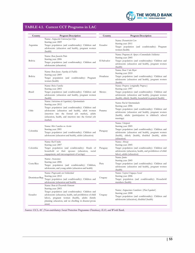
| 53
TABLE 4.1. Current CCT Programs in LAC
Sources: ECLAC (Non-contributory Social Protection Programmes Database), ILO, and World Bank.
Country Program Description Country Program Description
Argentina
Name: Asignación Universal por Hijo
Starting year: 2009
Target population (and conditionality): Children and
adolescents (education and health), pregnant women
(health)
Ecuador
Name: Desnutrición Cero
Starting year: 2011
Target population (and conditionality): Pregnant
women (health)
Bolivia
Name: Bono Juancito Pinto
Starting year: 2006
Target population (and conditionality): Children and
adolescents (education)
El Salvador
Name: Programa de Apoyo a Comunidades Solidarias
Starting year: 2005
Target population (and conditionality): Children and
adolescents (education and health), pregnant women
(health)
Bolivia
Name: Bono Juana Azurduy de Padilla
Starting year: 2009
Target population (and conditionality): Pregnant
women (health)
Honduras
Name: Bono Vida Mejor
Starting year: 2010
Target population (and conditionality): Children and
adolescents (education and health), pregnant women
(health)
Brazil
Name: Bolsa Família
Starting year: 2003
Target population (and conditionality): Children and
adolescents (education and health), pregnant women
(health)
Mexico
Name: Prospera (originally Progresa )
Starting year: 1997
Target population (and conditionality): Children and
adolescents (education and health), pregnant women
(health), elderly (health), household in general (health)
Chile
Name: Subsistema de Seguridad y Oportunidades
Starting year: 2012
Target population (and conditionality): Children and
adolescents (education and health), adult women
(insertion into the formal job market), adults
(education, health, and insertion into the formal job
market)
Panama
Name: Red de Oportunidades
Starting year: 2006
Target population (and conditionality): Children and
adolescents (education and health), pregnant women
(health), adults (participation in children's school
meetings)
Colombia
Name: Más Familias en Acción
Starting year: 2001
Target population (and conditionality): Children and
adolescents (education and health), adults (education)
Paraguay
Name: Tekoporâ
Starting year: 2005
Target population (and conditionality): Children and
adolescents (education and health), pregnant women
(health), elderly (health), disabled (health), adults
(education)
Colombia
Name: Red Unidos
Starting year: 2007
Target population (and conditionality): Heads of
household or their spouses (education, social
engagement, and encouragement of savings)
Paraguay
Name: Abrazo
Starting year: 2005
Target population (and conditionality): Children and
adolescents (education, health, and prohibition of child
labor), adults (education)
Costa Rica
Name: Avancemos
Starting year: 2006
Target population (and conditionality): Children,
adolescents, and young adults (education and health)
Peru
Name: Juntos
Starting year: 2005
Target population (and conditionality): Children and
adolescents (education and health), pregnant women
(health)
Dominican Rep.
Name: Progresando con Solidaridad
Starting year: 2012
Target population (and conditionality): Children and
adolescents (education and health)
Uruguay
Name: Tarjeta Uruguaya Social
Starting year: 2006
Target population (and conditionality): Household
members (health)
Ecuador
Name: Bono de Desarrollo Humano
Starting year: 2003
Target population (and conditionality): Children and
adolescents (education, health, and prohibition of child
labor), pregnant women (health), adults (family
planning education, and no dwelling in disaster-prone
areas)
Uruguay
Name: Asignaciones Familiares (Plan Equidad )
Starting year: 2008
Target population (and conditionality): Children and
adolescents (education), disabled (health)

54 | When Dreams Meet Reality
TABLE 4.2. Current Unemployment Insurance Programs in LAC
Sources: ECLAC, ILO, and World Bank.
Country Program Description
Argentina
Enactment year: 1991
Eligibility: Private salaried workers dismissed without just cause who have 6-8 monthly contributions to
social security.
Duration of coverage: 2-12 months. If the unemployed is 45+ years old, coverage is extended for 6 months.
Value of benefit: The benefit consists of a basic allowance plus the payment of family allowances, medical
coverage, and recognition of seniority for retirement. The basic allowance is variable, calculated as a
percentage of a reference value of half the best monthly net salary in the 6 months that preceded
unemployment, with decreasing monthly installments.
Brazil
Enactment year: 1986
Eligibility: Salaried workers dismissed without just cause who have 12 monthly contributions to Social
Security.
Duration of coverage: 3-5 months.
Value of benefit: The benefit consists of a basic allowance, which takes, as a reference, the average monthly
salary in the 3 months that preceded unemployment.
Chile
Enactment year: 2001
Eligibility: Private salaried workers. Workers may access the Individual Severance Account (ISA) and the
Solidarity Severance Fund (SSF). To access the ISA, workers must have at least 6-12 monthly
contributions, depending on the contract type, and at least 12 contributions in the case of the SSF.
Duration of coverage: 1-13 months in the ISA; 3-5 months in the SSF, depending on the contract type.
Value of benefit: The benefit consists of a basic allowance plus the payment of family allowances, medical
care coverage and recognition of seniority for retirement. The basic allowance is variable, with monthly
payments defined as percentages of an average monthly salary (of the last 6-12 months, depending on the
contract type).
Colombia
Enactment year: 2013
Eligibility: Workers that contributed to the Family Allowance Fund for 1-2 years during the 3 last years.
Duration of coverage: 6 months.
Value of benefit: Contributions to the health and pension systems (taking as base a legal minimum monthly
wage), a food bonus (of 1.5 times the legal minimum monthly wage, distributed equally for 6 months),
access to the prevailing family subsidy, and assistance in the search of new employment.
Ecuador
Enactment year: 2016
Eligibility: Salaried workers with (i) at least 24 contributions to the social security system (with the last 6
contributions in consecutive months), (ii) 60 days of unemployment, and (iii) involuntarily unemployment.
Duration of coverage: 5 months.
Value of benefit: The benefit consists of a basic allowance that varies per month, and is computed as a
percentage of the average monthly salary of the 12 months that preceded unemployment with decreasing
payments.
Uruguay
Enactment year: 1981
Eligibility: Unemployed or suspended private salaried workers.
Duration of coverage: 6 months in the case of dismissed workers, and 4 months in the case of suspended
workers.
Value of benefit: The benefit consists of a basic allowance that varies per month and is computed as a
percentage of the average salary of the 6 months that preceded unemployment with decreasing payments.
| 55
On average, unemployment insurance in the region offers benefits for up to 6 months, with payments
decreasing gradually over time to increase incentives for job search. In these countries, the average
gross replacement rate for the first year of unemployment is 20 percent, which is less than half the
OECD average.32 To make matters worse, given the eligibility requirements, only an average of 17
percent of the unemployed in these LAC countries receive unemployment benefits (with the average
falling to 6 percent if Chile and Uruguay are excluded). As discussed by the International Labour
Organization (2017) and Izquierdo et al. (2019), the high degree of informality is one of the main
factors limiting the collective funding of unemployment insurance schemes and, thus, the possibility
of increasing their coverage.
Behavior of CCT Programs throughout the Business Cycle
As argued above, the progressive expansion of social spending (particularly in the form of CCTs) since
the beginning of the Golden Decade is surely a key factor behind the large contribution of
redistributive policies to the reduction of poverty discussed in Chapter 3. It would thus prove useful
to study the behavior of real CCT spending in individual LAC countries to assess its sensitivity to the
business cycle. This is an important question because, in a region with limited shock absorbers (like
unemployment insurance), the fact that redistributive policies have contributed to poverty reduction,
even in recessions, may indicate that other social policies are acting, unintendedly, as shock absorbers.
Figure 4.2 displays the evolution of real CCT spending (normalizing the series to 100 in the first year)
for Argentina, Brazil, and Chile, and compares it with the cyclical component of real GDP (expressed
as a percentage of the trend). Except for the first two years of the implementation of each program,
recessionary periods (i.e., negative GDP cycle) are shaded. Although the recent starting date of CCT
programs limits the possibility of performing a systematic analysis throughout multiple business cycles,
the available information reveals two important messages:
• First, real CCT spending exhibits an upward trend with steep increases during economic
slowdowns, as reflected in Argentina (2014, Figure 4.2, Panel A), Brazil (2005-2006 and 2009,
Figure 4.2, Panel B), and Chile (2009-2011 and 2016-2017, Figure 4.2, Panel C). As discussed
in Izquierdo et al. (2019), the underlying force behind this phenomenon is that, as both
unemployment and poverty rise during recessions, a larger share of the population becomes
eligible for CCT benefits and takes advantage of these programs to compensate for the fall in
household income. Therefore, CCTs, which are de jure structural policy tools, become de facto
shock absorbers.
• Second, real CCT spending is rigid, especially downward. Figure 4.2 shows that once real CCT
spending expands, it is very unlikely to decrease. This is particularly the case for the steep
spending increases experienced during economic slowdowns (i.e., even after many years, real
CCT spending does not return to pre-recession levels). This has contributed to the significant
32 The average gross replacement rate is defined as the ratio of gross unemployment benefits received during one year over the yearly gross salary before inactivity.
56 | When Dreams Meet Reality
FIGURE 4.2. Real Expenditure in CCT Programs throughout the Business Cycle:
Argentina, Brazil, and Mexico
PANEL A. Argentina
PANEL B. Brazil
PANEL C. Chile
Note: Years with negative values in the real GDP cyclical component are shaded (except for the first two years of the implementation of the CCT program). Sources: ECLAC (Non-contributory Social Protection Programmes Database), ILO, and World Bank.
-4
-2
0
2
4
100
120
140
160
180
2010
2011
2012
2013
2014
2015
2016
2017
Rea
l GD
P C
ycle (
as p
erce
ntag
e of
Tre
nd)
Rea
l Expe
nditur
e in
CC
Ts
(20
10 =
100
)
Real Expenditure in CCTs Real GDP Cycle (right axis)
-4
-2
0
2
4
100
200
300
400
500
2003
2004
2005
2006
2007
2008
2009
2010
2011
2012
2013
2014
2015
2016
2017
Rea
l GD
P C
ycle (
as p
erce
ntag
e of
Tre
nd)
Rea
l Expe
nditur
e in
CC
Ts
(20
03 =
100
)
Real Expenditure in CCTs Real GDP Cycle (right axis)
-4
-2
0
2
4
100
450
800
1150
1500
2003
2004
2005
2006
2007
2008
2009
2010
2011
2012
2013
2014
2015
2016
2017
Rea
l GD
P C
ycle (
as p
erce
ntag
e of
Tre
nd)
Rea
l Expe
nditur
e in
CC
Ts
(20
03 =
100
)
Real Expenditure in CCTs Real GDP Cycle (right axis)
| 57
growth in the total expenditure of these programs, which has risen by a factor of 2, 5, and 15
times that of the first year in the case of Argentina, Brazil, and Chile, respectively. From the
perspective of the policymaker, both the de facto shock absorber function and rigidity of CCT
spending should be corrected to prevent the buildup of fiscal imbalances that may later
compromise the funding of the programs. If CCTs are intended to alleviate structural poverty,
then instances in which real CCT spending is suddenly cut down – such as fiscal adjustment
efforts in Argentina (2017, Panel A) and Brazil (2015-2017, Panel B) – should be avoided to
protect the most vulnerable. This downward rigidity is particularly evident since it has
occurred during a period of tremendous income growth.
In sum, the steady increase in social transfers has been an important driver of the prolonged
contribution of redistributive policy to poverty reduction in LAC. However, there are crucial caveats
that must be corrected so that each individual policy instrument can fulfill its intended role. In the
case of CCTs, efforts must be made to ensure that the programs are truly structural and target the
most vulnerable. In the case of shock absorbers, such as unemployment insurance, coverage must be
extended (which may require other policy efforts such as reducing informality). Only in this scenario
will each social instrument work as intended and the response of poverty to the business cycle be
greatly reduced.

58 | When Dreams Meet Reality

| 59
References
Adato, M., and J. Hoddinott (2010). Conditional Cash Transfers in Latin America (Baltimore: Johns
Hopkins University Press).
Ahluwalia, M., N. Carter, and H. Chenery (1979). “Growth and poverty in developing countries,”
Journal of Development Economics, Vol. 6, No. 3, pp. 299-341.
Alderman, H., U. Gentilini, and R. Yemtsov (2018). The 1.5 Billion People Question: Food, Vouchers, or
Cash Transfers? (Washington, DC: World Bank).
Alvaredo, F., and L. Gasparini (2015). “Recent Trends in Inequality and Poverty in Developing
Countries,” in A. Atkinson and F. Bourguignon, eds., Handbook of Income Distribution, pp. 697-805.
Atamanov, A., J.P. Azevedo, R.A. Castañeda, S. Chen, P.A. Corral Rodas, R. Dewina, C. Diaz-Bonilla,
D.M. Jolliffe, C. Lakner, K. Lee, D.G. Mahler, J. Montes, R. Mungai, M.C. Nguyen, E.B. Prydz, P.
Sangraula, K. Scott, A.E. Wambile, J. Yang, and Q. Zhao (2018). April 2018 PovcalNet Update: What’s
New (Washington, DC: World Bank).
Azevedo, J.P., M.E. Dávalos, C. Diaz-Bonilla, B. Atuesta, and R.A. Castañeda (2013). “Fifteen Years
of Inequality in Latin America: How Have Labor Markets Helped?” Working Paper 6384 (World
Bank).
Báez, J.E., and A. Camacho (2011). “Assessing the Long-term Effects of Conditional Cash Transfers
on Human Capital: Evidence from Colombia,” Working Paper 5681 (World Bank).
Báez, J.E., A. Fuchs, and C. Rodríguez-Castelán (2017). Shaking Up Economic Progress: Aggregate Shocks
in Latin America and the Caribbean (Washington, DC: World Bank).
Barrera-Osorio, F., M. Bertrand, L. Linden, and F. Perez-Calle (2008). “Conditional Cash Transfers
in Education: Design Features, Peer and Sibling Effects Evidence from a Randomized Experiment in
Colombia,” Working Paper 4580 (World Bank).
Barros, R., M. de Carvalho, S. Franco, and R. Mendonca (2010). “Markets, the State and the Dynamics
of Inequality in Brazil,” in L. López-Calva and N. Lustig, eds., Declining Inequality in Latin America: A
Decade of Progress? (Washington, DC: Brookings Institution Press and UNDP), pp. 134-174.
Bhalla, S. (2002). Imagine There’s No Country: Poverty, Inequality and Growth in the Era of Globalization
(Washington, DC: Institute for International Economics).
Bourguignon, F., and C. Morrison (2002). “Inequality among World Citizens: 1820-1992,” American
Economic Review, Vol. 92, No. 4, pp. 727-744.
Bourguignon, F. (2003). “The Growth Elasticity of Poverty Reduction: Explaining Heterogeneity
across Countries and Time Periods,” in T. Eicher and S. Turnovski, eds., Growth and Inequality (Boston:
MIT Press), pp. 3-26.
60 | When Dreams Meet Reality
Bühlmann, P. (2012). “Bagging, Boosting and Ensemble Methods,” in J.E. Gentle, W.K. Härdle, and
Y. Mori, eds., Handbook of Computational Statistics (Berlin: Springer-Verlag Berlin Heidelberg), pp. 985-
1022.
Campos, R., G. Esquivel, and N. Lustig (2012). “The Rise and Fall of Income Inequality in Mexico,
1989-2010,” WIDER Working Paper 2012/10 (United Nations University).
Cecchini, S., and A. Madariaga (2011). Conditional Cash Transfer Programmes: The Recent Experience in Latin
America and the Caribbean (Santiago de Chile: Economic Commission for Latin America and the
Caribbean).
Cruces, G., and L. Gasparini (2013). “Políticas Sociales para la Reducción de la Desigualdad y la
Pobreza en América Latina y el Caribe. Diagnóstico, Propuesta y Proyecciones en Base a la
Experiencia Reciente,” CEDLAS Working Paper 142 (Universidad Nacional de La Plata).
Datt, G., and M. Ravallion (1992). “Growth and Redistribution Components of Changes in Poverty
Measures,” Journal of Development Economics, Vol. 38, No. 2, pp. 275-295.
De la Torre, A., J. Messina, and S. Pienknagura (2012). The Labor Market Story Behind Latin America´s
Transformation (LAC Semiannual Report, World Bank).
Dubois, P., A. de Janvry, and E. Sadoulet (2012). “Effects on School Enrollment and Performance
of a Conditional Cash Transfer Program in Mexico,” Journal of Labor Economics, Vol. 30, No. 3, pp.
555-589.
Ferreira, F. (2012). “Distributions in Motion: Economic Growth, Inequality, and Poverty Dynamics,”
in P. Jefferson, ed., The Oxford Handbook of the Economics of Poverty (New York: Oxford University Press),
pp. 427-462.
Ferreira, F., J. Messina, J. Rigolini, L. López-Calva, M.A. Lugo, and R. Vakis (2013). Economic Mobility
and the Rise of the Latin American Middle Class (Washington, DC: World Bank).
Fiszbein, A., N. Schady, F. Ferreira, M. Grosh, N. Kelleher, P. Olinto, and E. Skoufias (2009).
Conditional Cash Transfers: Reducing Present and Future Poverty (Washington, DC: World Bank).
Gasparini, L., and G. Cruces (2010). “A Distribution in Motion: The Case of Argentina,” in L. López-
Calva and N. Lustig, eds., Declining Inequality in Latin America: A Decade of Progress? (Washington, DC:
Brookings Institution Press and UNDP), pp. 100-133.
Gasparini, L., M. Cicowiez., and W. Sosa Escudero (2013). Pobreza y Desigualdad en América Latina:
Conceptos, Herramientas y Aplicaciones (Buenos Aires: Editorial Temas).
Gasparini, L., G. Cruces, and L. Tornarolli (2016). “Chronicle of a Deceleration Foretold: Income
Inequality in Latin America in the 2010s,” CEDLAS Working Paper 198 (Universidad Nacional de La
Plata).
Gitter, S.R., and B.L. Barham (2009). “Conditional Cash Transfers, Shocks, and School Enrollment
in Nicaragua,” Journal of Development Economics, Vol. 45, No. 10, pp. 1747-1767.
| 61
International Labour Organization (2017). World Social Protection Report 2017-19 (Geneva: International
Labour Organization).
Inchauste, G., J.P. Azevedo, B. Essama-Nssah, S. Olivieri, T. Van Nguyen, J. Saavedra-Chanduvi, and
H. Winkler (2014). Understanding Changes in Poverty (Directions in Development - Poverty, World
Bank).
Izquierdo, A., J. Puig, C. Végh, and G. Vuletin (2019). “Automatic Destabilizers,” Unpublished
manuscript (Washington, DC: Inter-American Development Bank).
López-Calva, L., and N. Lustig (2010). Declining Inequality in Latin America: A Decade of Progress?
(Washington, D.C.: Brookings Institution Press).
Lustig, N., and D. McLeod (2011). “Inequality and Poverty Under Latin America’s New Left
Regimes,” Working Paper 1117 (Tulane University).
Lustig, N., L. López-Calva, and E. Ortiz-Juarez (2013). “Deconstructing the Decline in Inequality in
Latin America,” Working Paper 6552 (World Bank).
Maddison, A. (2009). Statistics on World Population, GDP and Per Capita GDP, 1-2008 AD (Groningen:
Groningen Growth and Development Centre).
Messina, J., and J. Silva (2018). Wage Inequality in Latin America: Understanding the Past to Prepare for the
Future (Washington, DC: World Bank).
Ravallion, M. (2016). The Economics of Poverty: History, Measurement, and Policy (New York: Oxford
University Press).
Rawlings, L.B., and G.M. Rubio (2005). “Evaluating the Impact of Conditional Cash Transfer
Programs,” The World Bank Research Observer, Vol. 20, No. 1, pp. 29-55.
Sala-i-Martin, X. (2006). “The World Distribution of Income: Falling Poverty and ... Convergence,
Period,” The Quarterly Journal of Economics, Vol. 121, No. 2, pp. 351-397.
Stampini, M., and L. Tornarolli (2012). “The Growth of Conditional Cash Transfers in Latin America
and the Caribbean: Did They Go Too Far?” IZA Policy Paper 49 (Institute of Labor Economics).
Shapley, L. (1953). “A Value for n-Person Games,” Annals of Mathematics Studies, No. 28, pp. 307-317.
United Nations Refugee Agency and International Organization for Migration (2019). Regional Refugee
and Migrant Response Plan for Refugees and Migrants from Venezuela (Geneva: United Nations Refugee
Agency and International Organization for Migration).
World Bank (2018a). Migración desde Venezuela a Colombia: Impactos y Estrategia de respuesta en el Corto y
Mediano Plazo (Washington, DC: World Bank).
World Bank (2018b). Poverty and Shared Prosperity 2018: Piecing Together the Poverty Puzzle (Washington,
DC: World Bank).
Végh, C.A., L. Morano, D. Friedheim, and D. Rojas (2017). Between a Rock and a Hard Place: The
Monetary Policy Dilemma in Latin America and the Caribbean (LAC Semiannual Report, World Bank).

62 | When Dreams Meet Reality
Végh, C.A., G. Vuletin, D. Riera-Crichton, J. P. Medina, D. Friedheim, L. Morano, and L. Venturi
(2018). From Known Unknowns to Black Swans: How to Manage Risk in Latin America and the Caribbean
(LAC Semiannual Report, World Bank).

| 63
Appendices
Appendix A: Annual Growth for LAC Countries
TABLE A.1. Annual Real GDP Growth Rates for LAC Countries
Notes: Regional and sub-regional figures are weighted averages. Weights are calculated using WEO’s 2017 GDP. “f” stands for forecast. Data as of March 15th, 2019. Sources: World Bank staff estimates (March 2019) when available, otherwise WEO (October 2018).
Region Country 2016 2017 2018 2019f 2020f
SA Argentina -1.8 2.9 -2.5 -1.3 2.9
Brazil -3.3 1.1 1.1 2.2 2.5
Bolivia 4.3 4.2 4.0 4.0 3.6
Chile 1.3 1.5 4.0 3.5 3.1
Colombia 2.0 1.8 2.7 3.3 3.7
Ecuador -1.2 2.4 1.2 0.1 0.4
Guyana 2.6 2.1 3.4 4.6 33.7
Paraguay 4.3 5.0 3.8 3.6 4.0
Peru 4.0 2.5 4.0 3.8 3.9
Suriname -5.6 1.4 2.0 2.0 2.1
Uruguay 1.7 2.7 2.1 1.8 2.7
Venezuela, RB -16.5 -14.5 -17.7 -25.0 n/a
MEX Mexico 2.9 2.1 2.0 1.7 2.0
CA Belize -0.6 1.4 2.8 2.3 2.1
Costa Rica 4.2 3.2 2.7 3.0 3.1
El Salvador 2.6 2.3 2.6 2.6 2.5
Guatemala 3.1 2.8 3.0 3.3 2.7
Honduras 3.9 4.8 3.5 3.6 3.8
Nicaragua 4.7 4.9 -3.8 -5.0 1.1
Panama 5.0 5.3 3.7 6.0 5.4
CB Antigua and Barbuda 5.3 3.3 2.7 2.7 2.7
The Bahamas -1.7 1.4 1.8 1.9 2.0
Barbados 2.0 1.7 1.6 1.6 1.6
Dominica 2.5 2.7 -9.5 0.5 7.0
Dominican Republic 6.6 4.6 7.0 5.2 5.0
Grenada 3.7 5.1 5.2 3.9 3.7
Haiti 1.5 1.2 1.5 0.4 1.6
Jamaica 1.4 1.0 1.7 1.6 1.7
St. Kitts and Nevis 2.2 1.7 6.9 6.9 6.9
St. Lucia 3.9 3.7 1.5 3.4 3.5
St. Vincent and the Grenadines 1.3 0.7 2.0 2.1 2.3
Trinidad and Tobago -6.5 -1.9 -1.0 -0.5 2.0
LAC -0.9 1.3 0.7 0.9 n/a
South America (SA) -2.5 0.8 0.1 0.4 n/a
Mexico, Central America, and the Caribbean (MCC) 3.1 2.4 2.3 2.1 2.4
Central America (CA) 3.9 3.7 2.7 3.4 3.5
Caribbean (CB) 2.7 2.6 4.0 3.2 3.6
Real GDP Growth (as percentage)

64 | When Dreams Meet Reality
Appendix B: Level of Governments
TABLE B.1. Level of Government for LAC Countries
Source: World Bank staff (March 2019).
Country Level of Government
Argentina General Government
Brazil General Government
Bolivia Non-Financial Public Sector
Chile General Government
Colombia General Government
Ecuador Non-Financial Public Sector
Guyana Central Government
Paraguay Consolidated Public Sector
Peru Non-Financial Public Sector
Suriname Central Government
Uruguay Non-Financial Public Sector
Venezuela, RB Non-Financial Public Sector
Mexico Federal Public Sector Borrowing Requirements
Belize Central Government
Costa Rica General Government
El Salvador Non-Financial Public Sector
Guatemala Central Government
Honduras Non-Financial Public Sector
Nicaragua Non-Financial Public Sector
Panama Non-Financial Public Sector
Antigua and Barbuda General Government
The Bahamas General Government
Barbados General Government
Dominica General Government
Dominican Republic Non-Financial Public Sector
Grenada General Government
Haiti Non-Financial Public Sector
Jamaica Central Government
St. Kitts and Nevis General Government
St. Lucia Central Government
St. Vincent and the Grenadines Central Government
Trinidad and Tobago Central Government
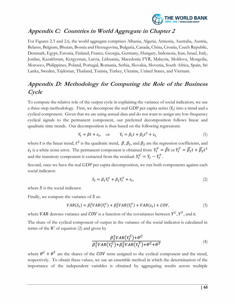
| 65
Appendix C: Countries in World Aggregate in Chapter 2
For Figures 2.3 and 2.6, the world aggregate comprises Albania, Algeria, Armenia, Australia, Austria,
Belarus, Belgium, Bhutan, Bosnia and Herzegovina, Bulgaria, Canada, China, Croatia, Czech Republic,
Denmark, Egypt, Estonia, Finland, France, Georgia, Germany, Hungary, Indonesia, Iran, Israel, Italy,
Jordan, Kazakhstan, Kyrgyzstan, Latvia, Lithuania, Macedonia FYR, Malaysia, Moldova, Mongolia,
Morocco, Philippines, Poland, Portugal, Romania, Serbia, Slovakia, Slovenia, South Africa, Spain, Sri
Lanka, Sweden, Tajikistan, Thailand, Tunisia, Turkey, Ukraine, United States, and Vietnam.
Appendix D: Methodology for Computing the Role of the Business
Cycle
To compute the relative role of the output cycle in explaining the variance of social indicators, we use
a three-step methodology. First, we decompose the real GDP per capita series (𝑌𝑡) into a trend and a
cyclical component. Given that we are using annual data and do not want to assign any low-frequency
cyclical signals to the permanent component, our preferred decomposition follows linear and
quadratic time trends. Our decomposition is thus based on the following regressions:
𝑌𝑡 = 𝛽𝑡 + 𝜀𝑡 , or 𝑌𝑡 = 𝛽1𝑡 + 𝛽2𝑡2 + 𝜀𝑡, (1)
where 𝑡 is the linear trend, 𝑡2 is the quadratic trend, 𝛽, 𝛽1, and 𝛽2 are the regression coefficients, and
𝜀𝑡 is a white noise error. The permanent component is obtained from 𝑌𝑡𝑇 = �̂�𝑡 or 𝑌𝑡
𝑇 = 𝛽1̂𝑡 + 𝛽2̂𝑡2
and the transitory component is extracted from the residual: 𝑌𝑡𝐶 = 𝑌𝑡 − 𝑌𝑡
𝑇.
Second, once we have the real GDP per capita decomposition, we run both components against each
social indicator:
𝑆𝑡 = 𝛽1𝑌𝑡𝐶 + 𝛽2𝑌𝑡
𝑇 + 𝜀𝑡 , (2)
where 𝑆 is the social indicator.
Finally, we compute the variance of 𝑆 as:
𝑉𝐴𝑅(𝑆𝑡) = 𝛽12𝑉𝐴𝑅(𝑌𝑡
𝐶) + 𝛽22𝑉𝐴𝑅(𝑌𝑡
𝑇) + 𝑉𝐴𝑅(𝜀𝑡) + 𝐶𝑂𝑉, (3)
where 𝑉𝐴𝑅 denotes variance and 𝐶𝑂𝑉 is a function of the covariances between 𝑌𝐶 , 𝑌𝑇, and 𝜀.
The share of the cyclical component of output in the variance of the social indicator is calculated in
terms of the R2 of equation (2) and given by
𝛽12𝑉𝐴𝑅(𝑌𝑡
𝐶)+𝜃𝐶
𝛽12𝑉𝐴𝑅(𝑌𝑡
𝐶)+𝛽22𝑉𝐴𝑅(𝑌𝑡
𝑇)+𝜃𝐶+𝜃𝑇 (4)
where 𝜃𝐶 + 𝜃𝑇 are the shares of the 𝐶𝑂𝑉 term assigned to the cyclical component and the trend,
respectively. To obtain these values, we use an ensemble method in which the determination of the
importance of the independent variables is obtained by aggregating results across multiple
66 | When Dreams Meet Reality
models.33 All possible ensemble combinations with two independent variables in the full model result
in two estimated models. By alternating each independent variable between included versus excluded,
the final shares are derived as a weighted average marginal/incremental contribution to the overall fit
made by an independent variable across all models in which the independent variable is included.
These values are equivalent to Shapley values (Shapley, 1953). Since the shares of the variance of the
social indicators explained by the output cycle and output trend are reported in relation to the R2 of
regression (2), they will add up to 1 (i.e., 100 percent of the R2).
Appendix E: Poverty Data
Most of the data for monetary poverty comes from PovcalNet, an interactive computational tool that
allows users to replicate the calculations made by World Bank researchers when estimating the extent
of absolute poverty in the world.34
The PovcalNet data for LAC are taken from the Socio-Economic Database for Latin America and
the Caribbean (SEDLAC). SEDLAC was developed by the Center for Distributional, Labor, and
Social Studies (CEDLAS) of the Universidad Nacional de La Plata (Argentina), in partnership with
the Latin America team of the World Bank’s Poverty and Equity Group. Methodological and technical
revisions to the SEDLAC project began in 2015 to better align its data with the household surveys
harmonized by the World Bank for other regions. These revisions of the welfare aggregate constitute
the move of the SEDLAC project from version 02 to version 03.35
As the revision of this project is still in process, data reported in PovcalNet are based on SEDLAC-
03 for most recent years and on SEDLAC-02 for previous years, with the cut-off period being
generally the year 2000 (except for Argentina, for which data using SEDLAC-03 begins in 2003, and
Chile, which uses SEDLAC-02 throughout the whole period). Given this problem of comparability,
we recalculate headcount ratios for some countries so that the SEDLAC version used in each country
is the same for the whole period under analysis.36
We focus on measures of poverty in the income space using international poverty lines in dollars
adjusted for purchasing power parity (PPP). The World Bank Group pursues the end of extreme
poverty in the world by 2030, which implies decreasing the number of people living on less than 1.90
dollars per day (2011 PPP) to less than 3 percent of the global population. Since most countries in
LAC have low extreme poverty rates, the level of economic development in the region has led analysts
33 See, for example, Bühlmann (2012).
34 As of the writing of the core of this report, the PovcalNet database had not yet been updated and, hence, we used the September 2018 version. The only exception is Figure 1.15, for which we could use the March 2019 version. In any event, preliminary calculations indicate that changes would be extremely small, if any.
35 For details on the main methodological changes in SEDLAC-03 that directly affect welfare measurement, see Atamanov et al. (2018).
36 Notice that even though the SEDLAC project may remain the same, the frequent changes in survey methodologies over time introduce comparability issues with previous surveys that are difficult to deal with. In addition, there are comparability issues across countries since national agencies often use different survey standards. However, we can still draw general conclusions from the available data.

| 67
to use regional poverty lines that are higher and more consistent with individual countries’ official
thresholds for extreme and moderate monetary poverty: 3.20 dollars per day and 5.50 dollars per day
(2011 PPP). In particular, most of this report focuses on the 5.50 dollars per person a day (2011 PPP).
The data series for monetary poverty in Colombia, Dominican Republic, and Ecuador are exactly the
same as the ones reported in PovcalNet (SEDLAC-03, September 2018). In Brazil, Costa Rica,
Mexico, Panama, Peru, and Uruguay, the data series for monetary poverty since 2000 are the same as
in PovcalNet (SEDLAC-03, September 2018), but older data are estimated with microdata from
SEDLAC-03 because data from PovcalNet for this period corresponds to SEDLAC-02.37 38
Given that there are some countries for which we do not have poverty estimates or microdata
harmonized using SEDLAC-03 for the entire period under analysis, we use SEDLAC-02 in these
cases to gain comparability over time. These countries are Argentina, Bolivia, Chile, Honduras,
Paraguay, and El Salvador. We use data from PovcalNet (September 2018), computed using
SEDLAC-02, for the first years (until 1999 in most countries, except for Argentina, where we use
PovcalNet data until 2002), and estimate poverty measures using SEDLAC-02 for the subsequent
years, because PovcalNet’s data for this period are based on SEDLAC-03.39 40
Finally, as the version of the PovcalNet database we use (September 2018) does not include 2017 for
the countries under analysis, we estimate monetary poverty in this year using microdata from
SEDLAC-03. It is worth mentioning that the figures we obtain are the same as those reported in the
latest update in PovcalNet (March 2019) for the years with available microdata. Therefore, the
methodology applied in this report is consistent with the estimations presented in this source.
Table E.1 summarizes the data used for each country. As the table makes clear, we use the latest
version available in 9 out of 15 countries.
37 In cases where there is no harmonized microdata available using SEDLAC-03, we rely on data from PovcalNet and apply the growth rates reported in this source to our data. This strategy applies to the following countries and years: Costa Rica 1989, Mexico 1989, Panama 1989, Peru 1994, and Uruguay 1989.
38 We exclude Mexico 2016 from the analysis because there is a methodological change in the survey that considerably affects welfare measurements.
39 Since the last year with available harmonized microdata based on SEDLAC-02 is 2015, we apply the growth rates in SEDLAC-03 to our data for the years 2016 and 2017.
40 An exception is Chile, as it has data in PovcalNet based on SEDLAC-02 for the entire period, but we opt to use an older version that improves comparability over time.
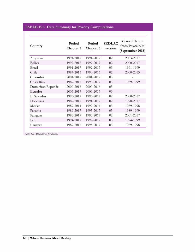
68 | When Dreams Meet Reality
TABLE E.1. Data Summary for Poverty Computations
Note: See Appendix E for details.
CountryPeriod
Chapter 2
Period
Chapter 3
SEDLAC
version
Years different
from PovcalNet
(September 2018)
Argentina 1991-2017 1991-2017 02 2003-2017
Bolivia 1997-2017 1997-2017 02 2000-2017
Brazil 1991-2017 1992-2017 03 1991-1999
Chile 1987-2015 1990-2015 02 2000-2015
Colombia 2001-2017 2001-2017 03 -
Costa Rica 1989-2017 1990-2017 03 1989-1999
Dominican Republic 2000-2016 2000-2016 03 -
Ecuador 2003-2017 2003-2017 03 -
El Salvador 1995-2017 1995-2017 02 2000-2017
Honduras 1989-2017 1991-2017 02 1998-2017
Mexico 1989-2014 1992-2014 03 1989-1998
Panama 1989-2017 1995-2017 03 1989-1999
Paraguay 1995-2017 1995-2017 02 2001-2017
Peru 1994-2017 1997-2017 03 1994-1999
Uruguay 1989-2017 1995-2017 03 1989-1998

THE WORLD BANK1818 H STREET NW
WASHINGTON, DC 20433, USA
WWW.WORLDBANK.ORG/LACECONOMIST


