Regional Trade Agreements for MERCOSUR: the FTAA and the FTA with the European Union1

Josefina Monteagudo Masakazu Watanuki2

October 2001

DRAFT FOR COMMENTS

PLEASE DO NOT DISTRIBUTE WITHOUT THE AUTHORS’ CONSENT

1 Paper prepared for presentation at the Conference “Impacts of Trade Liberalization Agreements on Latin America and the Caribbean”, organized by the Inter-American Development Bank and the Centre d’Etudes Prospectives et d’Information Internationales, November 5-6, 2001, Washington, DC. 2 The authors are economists at the Department of Integration and Regional Programs of the Inter-American Development Bank. They thank Reuben Kline for superb research assistance. The opinions expressed are those of the authors and not necessarily those of the Inter-American Development Bank.

1. Introduction

Regional integration provides a promising answer for developing countries to the challenge of

opening their markets to international trade. MERCOSUR countries adopted this strategy and, since the

signing of the Treaty of Asuncion in 1991, they have aimed to consolidate their integration efforts.

During the nineties the bloc eliminated most of the trade barriers among them and established an “almost

perfect” customs union (CU). For a decade the group achieved one of the highest levels of integration in

Latin America; however, the economic slowdown in the region in the last couple years, and especially in

Argentina, has put a halt to that virtuous process which brought fast export growth and promoted export

diversification among its members.

Preferentialism is not just a question of comparing economic costs and benefits, since it calls for non-

economic as well as economic considerations. The negotiations involving a free trade area (FTA) with the

European Union (EU) and talks for a free trade area in the Americas (FTAA) remind us that

MERCOSUR can be a powerful tool to maximize scale advantages as well as to increase the countries’

bargaining power in broader regional agreements. Acknowledging this fact, the four member countries

have usually negotiated, since the beginning of MERCOSUR, as a joint bloc in the international arena. In

fact, MERCOSUR seeks an international agenda that, in a context of increasing global interdependence,

would enable the bloc to successfully respond and adapt to the changing outside world. The policymakers

face an FTAA and an FTA with the EU as the two broadest schedules under negotiation. Both agreements

will bring about large gains in both trade and GDP growth to MERCOSUR countries, but also substantial

structural changes with important domestic economic and political implications. Having good ex-ante

knowledge of the anticipated structural transformations is an excellent tool at the negotiation table as well

as at home.

In this paper, we analyze the economic impact on MERCOSUR countries of these two FTAs

(individually and simultaneously considered) using a computable general equilibrium (CGE) model. We

use a multi-country, multi-sector, and comparative static model benchmarked in 1997. The model

incorporates trade-linked externalities that increase efficiency in the production process in all sectors.

Many authors have shown how important economies of scale can be in assessing the results of trade

liberalization. In this spirit, the model also incorporates economies of scale in the manufacturing sectors,

thus allowing countries to take further advantage of the scale of the new market created.

As in most models dealing with trade liberalization, we use tariff elimination as one of the main trade

policy variables. However, tariff protection is already fairly low in most countries (agriculture in the EU

being an exception with important consequences for MERCOSUR), and most protection now comes from

non-tariff barriers (NTBs). In order to have a model as close to reality as possible, we incorporate NTBs

as an additional trade policy variable. However, the accurate estimation of the NTBs is not an easy task

and we borrow estimations from the literature for the EU, Mexico, Canada and the United States.

The empirical results show the large trade creation generated by the two agreements. But we also

observe significant trade diversion away from extra-regional partners when tariffs are removed (which is

not the case when NTBs are also removed). We find that the introduction of the NTBs makes the FTAA a

better option for MERCOSUR countries than the FTA with EU, reversing the ranking from the tariff-only

scenario. The elimination of NTBs greatly increases the factor reallocation impact and, thus, the structural

adjustment in MERCOSUR countries being an indication for policy makers of the importance of gaining

a complete market access in a negotiation agreement.

Another related finding is the fact that the Hemispheric integration promotes exports with higher

value-added than integration with the European market. However, in relative terms, exports to Latin-

American partners in the FTAA agreement are more valued-added exports than exports to the US market

(especially for Brazil). Since policy-makers may be interested in identifying the effects on sensitive

sectors and targeting key dynamic industries, these sectoral results are extremely useful.

We note that the benefits of the realization of economies of scale in manufactures spill over to other

sectors as output further grows in all industries, except machinery and equipment in Argentina which

contracts. In addition, the additional gains are evenly distributed across sectors. This should not come as a

surprise since MERCOSUR countries are not the only countries that can benefit from the potential

realization of economies of scale in manufactures.

The rest of the paper is organized as follows. Section 2 presents the model and its main

characteristics. Section 3 describes the data sources and analyses the countries’ trade and production

structure at the benchmark year. Section 4 describes in detail the scenarios and different versions

considered in the paper. Section 5 deals with the results and contains an aggregated and detailed analysis.

Finally, Section 6 concludes the analysis.

2. The MERCOSUR CGE Model

This section presents a brief description of the MERCOSUR CGE model. The model is a multi-

region, multi-sector and static general equilibrium model with 15 sectors 12 regions that follows the

standard theoretical specifications of trade-focused CGE models. All regions are fully endogenized,

including the rest of the world, and linked through trade. The model deals with the real side of the

economy and therefore does not consider financial or monetary markets. The base year used is 1997.

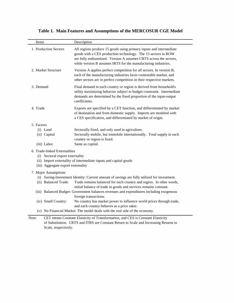
Table 1 summarizes the main features and assumptions underlying the model that we describe in some

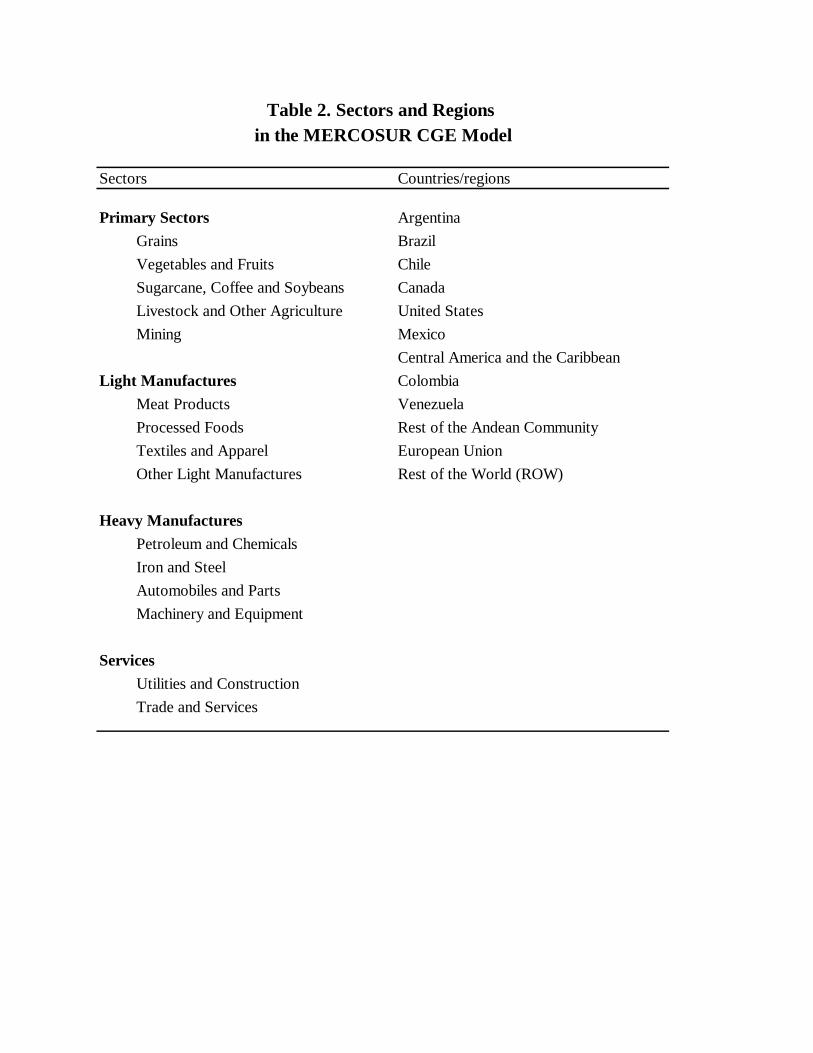
detail next and Table 2 contains the sectors and regions.3

<INSERT TABLE 1 and 2>

The model used has some salient features giving it an advantage over conventional multi-region CGE

models for MERCOSUR. It identifies key industries and partners of MERCOSURs external agenda and

incorporates the latest trade agreements in effect in the Western Hemisphere: US preferential trade

arrangements with Latin American countries (CBI, Andean Trade Preferences Act), bilateral agreements

(MERCOSUR-Chile, Chile-Canada, Mexico-Chile), and regional agreements (MERCOUSUR, NAFTA,

EU, CACM and CARICOM, Andean Community, and G-3 among Mexico, Colombia and Venezuela).

These are very important elements to take into account in order to evaluate accurately any integration

policy.

In addition, the MERCOSUR CGE model extends beyond standard static CGE models in two

directions. First, it incorporates trade-related externalities that induce efficiency gains as a result of

increased trade. It is widely acknowledged that a greater liberalization has dynamic effects resulting from

economies of scale, technical changes, technological spillover, specialization and increased investment

(Lewis, Robinson and Wang, 1995). Today this is a crucial element in Latin America where trade, namely

exports, has become an important source of growth and foreign currency earnings and a key policy

variable. In order to capture some of these dynamic effects, the model draws the theoretical structure from

Melo and Robinson (1992), and follows the work of Hinajosa-Ojeda, Lewis and Robinson (1995, 1997)

on Western Hemisphere integration in its empirical implementation.4

3 Due to their economic size and trade flows, Argentina and Brazil represent MERCOSUR in the paper. 4 We also rely on our previous work (Monteagudo and Watanuki, 2001) in which we evaluate a broader set of MERCOSUR’s integration alternatives.

The model includes three types of trade-productivity links. The first one is a sectoral export

externality linked to sectoral export performance. Higher export growth leads to an increase in domestic

productivity at the sectoral level. The second one is an externality associated with import of intermediate

inputs and capital goods. The degree of efficiency gains depends on the import share of intermediates

and capital goods in production. The last one is an aggregate export externality; in this case, an increase

in total exports raises the physical productivity of capital, embedded in the capital stock, thereby leading

to economy-wide efficiency gains in the production process.

The three externalities are expressed in equations (1)-(3). kiEK is sectoral exports where i represents

the sector and k the region, kETOT and kMTOT correspond to the aggregate exports and imports in

each region. The exponents keη , kmη and kkη are the externality elasticities, and in is the import share

of intermediate inputs and capital goods. The subscript 0 refers to the benchmark. Thus, the growth of

sectoral exports increases productivity in each of the exporting sectors (equation 1); the growth of

aggregated imports yields to a larger productivity parameter in all sectors (equation 2); and the growth of

aggregate exports increases capital productivity (equation 3).

(1) Sectoral export externality: ( ) keki

ki

ki EKEKSAD

η0/=

(2) Import externality: ( ) )1(/2 0 i

mkki

ki nMTOTMTOTnSAD

k

−+⋅=η

(3) Aggregate export externality: ( ) kkkkki ETOTETOTSAC

η0/=

Specifically, the sectoral export performance externality )( kiSAD and import externality

)2( kiSAD are included in the primary variable cost function and factor demands equations derived from

the firm’s optimization behavior (they reduce production cost and improve efficiency in the use of factors

of production, thus reducing its demand). The aggregate export externality )( kiSAC improves capital

productivity, which is embedded in the capital stock.

The externalities’ elasticities are key parameters that will influence the simulation results. For this

paper, we used estimations from the work of Mauricio and Najberg (2000) on the productivity analysis of

Brazilian manufacturing industries in 1990-97, the most expansionary phase of the dynamic MERCOSUR

integration process. The parameter values are estimated from sectoral trade data in that period for Brazil

and are applied to other regions in Latin America in the model, adjusted with trade flows as weights. For

developed countries, the parameters were estimated on the basis of the productivity growth analysis by

Roberts (2000) and Stiroh (2001) for the United States. For Canada and the European Union, we

sectorally adjust the estimations by Lewis, Robinson and Wang (1995), and Hinojosa-Ojeda, Lewis and

Robinson (1997). In all regions the trade externalities’ elasticities estimations are larger in manufacturing

sectors than in agricultural ones.

The second extension of the model is the inclusion of economies of scale in manufacturing industries.

Following the pioneering work by Harris (1984), the nature of industrial organization—scale economies,

imperfect competition, and product differentiation—has been introduced into the static framework, and

applied to the evaluation of trade liberalization (Rodrik, 1988; Gunasekara, 1991; Melo and Tarr, 1992).

Some applications for multi-region models include Roland-Holst, Reinert and Shiells (1994) for NAFTA,

Harrisson, Rutherford and Tarr (1994) and Brown, Deardorff and Stern (1998) for the Chile’s accession

to NAFTA and hemispheric integration. On MERCOSUR, Flores (1997) examined the trade policy

scenarios using the multi-region static model with imperfect competition and scales economies.

The degree of economies of scale is specified with one parameter, the cost disadvantage ratio (CDR),

which is defined by the difference between average cost (AC) and marginal cost (MC) over average cost

for the industry or representative firm in each sector. With a simple algebraic transformation CDR then

becomes the ratio of fixed cost (FC) over total cost (TC):

(4) Cost disadvantage ratio: ki

ki

ki

ki

kik

i TCFC

ACMCACCDR =

−=

The larger the CDR, the greater the potential gains from trade liberalization due to the realization of

scale economies. The estimates of the CDR are obtained from cost structure data on manufacturing

industries for Brazil, Mexico and the United States, and they are also applied to other countries or regions

in the Western Hemisphere, after some adjustments. The estimates for the European Union are drawn

directly from the work of Harrison, Rutherford, and Tarr (1994).

The presence of scale of economies has implications for the market structure since perfect

competition is not possible. The simplest way to deal with increasing returns to scale (IRTS) in the CGE

model has traditionally been assuming contestable markets, since that implies a structure analogous to the

perfect competition in the presence of constant returns to scale (CRTS). Contestable market assumes low-

cost entry or exit and that the threat of entry drives the incumbent firm to behave competitively so that it

sets the price at average costs.5 The pricing rule for contestable market is defined in equation 5:

(5) Contestable market pricing: kik

i

kik

i ACX

TCPX ==

where PX is the unit prices of domestic output by sector. Thus, the average cost pricing under the

contestable market, similar to the competitive case, implies that no firm will enter the industry. Since the

number of firms per industry is constant, the efficiency gains are directly influenced by industry output

(as firms move down its average cost curve) and by the trade externalities arising from increased trade;

thus if trade liberalization leads to an expansion of output, the incumbent firms will increase production

while lowering their average costs. In this paper we also assume that there are not initial profits for the

industries. Scale economies are present only in manufacturing industries, while the other industries in the

economy are modeled according to the CRTS assumption. Figure 1 illustrates the pricing and cost

structure in the contestable markets of the model following the common assumption in other studies of

constant marginal cost.

<INSERT Figure 1>

In addition to the 15 sectors in each region, the model includes three factors of production: labor,

capital and land. Output is produced with a constant elasticity of substitution (CES) technology for the

variable cost component that comprises primary factors and intermediate inputs in fixed proportions. The

variable cost function (CV) is derived from the cost minimization by the representative firm using primary

inputs and intermediates subject to the technology constraint. Factor returns (wages, capital rent and land

prices) are not assumed to be uniform across sectors, as factor market rigidities or distortions are assumed

to be present. We model such distortions by using the factor returns differential (wfdist) observed in the

benchmark data. As mentioned above, scale economies are modeled by introducing a fixed cost

component in the cost function so that the total cost function for the sectors with IRTS is:

(6) Total cost: k

iki

ki CVFCTC +=

5 Other ways of modeling imperfect competitive markets in the literature include: assuming that firms behave like in a Cournot oligopoly market (conjectural variations) in which case they apply a mark-up pricing policy; or assuming product differentiation in a monopolistic competition framework. Due to data availability at this stage of the paper we only use the contestable market case.

where the fixed cost component is estimated by multiplying the CDR (equation 4) by the total cost. Under

the assumption of uniform factor share between the fixed and value-added components, we derive the

factor demands associated with each component.6

Both labor and capital in the variable cost component are completely mobile across the sectors, but

immobile internationally. Factors allocated to the fixed cost component are by definition fixed at the

benchmark level. Land is a sector-specific factor and is only used in agriculture. The aggregate supply of

capital and labor is exogenously fixed in each region. It is important to notice that although the

introduction of trade externalities and IRTS in the model will clearly lead to a higher output expansion

after a trade liberalization, the effects on resource allocation are, ex-ante, ambiguous, being that this is

merely an empirical question. For example, factor demand per unit of output decreases as externalities

enter into play, especially in manufacturing industries, but the overall factor demand per industry depends

also on the effects on total output (that depends on other elements such as trade-externalities and degree

of economies of scale in other countries, sectoral initial protection, etc.)

The treatment of international trade follows standard CGE modeling assumptions. That is, the model

specifies a set of export-supply and import-demand equations for traded sectors, which are imperfect

substitutes. Exports are modeled with a constant elasticity of transformation (CET) between domestic

sales and exports. Producers optimally allocate sales between the domestic market and exports to the

respective partners in order to maximize revenue from total sales. Following the “Armington”

assumption, imports are modeled by a CES function, implying that imports from different sources are

differentiated each other by country of origin. The rest of the world is modeled as a large supplier of

imports to each of the 11 regions and a demander of exports from these regions at the fixed world market

prices.

In common with other CGE models, the MERCOSUR model only determines relative prices and

therefore needs to specify the absolute price level exogenously. In the model, the aggregate consumer

price index in each region is set exogenously, defining the numeraire. With this specification, equilibrium

goods prices, wages and other factor rents as well as exchange rate are measured in real terms. World

prices are converted into domestic currencies using nominal exchange rates, and adjusted through market

distortions such as tariffs, export taxes or subsidies.

6 This process allows for the same factor returns between fixed cost and variable cost (See Appendix A in Melo and Tarr, 1992).

As with most of the static models, the MERCOSUR model has three key macro closures: saving-

investment identity, balance of trade, and balanced public budget. Investment is completely financed by

savings which, in the model, come from four sources: private (households), firms, government and

external borrowing. The saving rate for firms is fixed constant and government savings are determined as

residual between its receipt and expenditures, while the marginal propensity to save for households is

allowed to adjust to achieve the saving-investment equality. Trade is also balanced for each region,

valued at world prices, and exchange rates in each region are required to vary to achieve external balance

in the respective regions. In other words, initial balance of trade (in goods and services) remains constant.

Finally, the government also maintains a balanced budget. Since some of the expenses and revenues items

are set exogenously (for example, government consumption is kept constant in real terms as well as

foreign borrowing) other items has to adjust to keep the budget balanced (for example, taxes—indirect

taxes, direct taxes from households and firms, commodity taxes, social security taxes, tariffs and export

taxes from external transactions—are all endogenized).

3. Data Sources and Economic Structure at Benchmark

3.1.Data Sources The MERCOSUR CGE model is constructed on the basis of the individual country/region Social

Accounting Matrix (SAM), benchmarked in 1997. SAM, which displays a comprehensive snapshot of the

economies, is used to derive the economy-wide income-expenditure balance subject to the underlying

budget constraints by each institution.

Since the policy parameter in this paper is the elimination of the existing trade protection (ad valorem

tariff and NTBs) and trade flows are the key elements to transmit the effects among partners, it is of vital

importance to estimate these data as accurately as possible. To this end, we used DATAINTAL, FTAA

and the OECD database for bilateral trade flows aggregated into 15 sectors. Trade protection data (tariff)

comes from several sources: official country data for MERCOUSR (Argentina and Brazil), FTAA

database for other Latin American Countries or regions, and UNCTAD database for the European Union.

Trade liberalization analysis that only focuses on tariff elimination underestimates, in general, the overall

effects of trade policy. Although some attempts have been made to correct this shortcoming, this is no

doubt an area clearly in need of improvement. Based on the estimations made by other studies, we

incorporate in the paper a tariff equivalent quantification of the NTBs only for Canada, the US, Mexico

and the EU.7

7 Bussolo and Roland-Holst (1998) for Canada, United States, and Mexico. For the European Union, NTBs are from Lewis, Robinson and Wang (1995) with some adjustment.

Industrial data to estimate the CDR are drawn from the literature and available for four

countries Brazil, Mexico, the United States, and the European Union and the parameter values for

other Latin American countries are averaged from these industrial date in the Hemisphere.8 Other data

sources include International Financial Statistics (IMF) for national accounts, Government Finance

Statistics (IMF) for public finance, Industrial Statistics (UNIDO) for industrial production, and Labor

Statistics (ILO) for sectoral employment and wages. Finally, the model applies the input-output tables

provided from Argentina (1997) and Brazil (1990) in the construction of the country SAMs. For other

countries and regions, we used the I-O data from the GTAP (version 5) as reference. Final adjustment to

balance the corresponding rows and columns in each account is made through RAS procedure.9

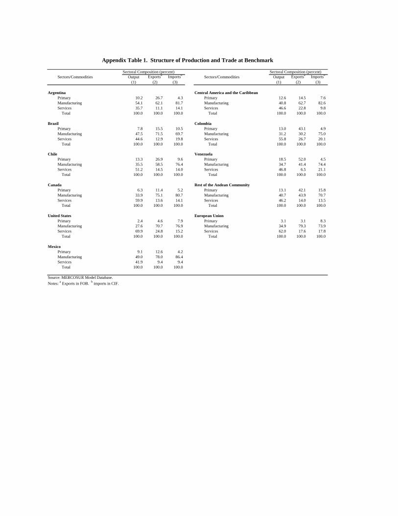
3.2 Economic Structure at Benchmark

A close look at the structure of production, trade and protection of the countries in the base year is

crucial in understanding the simulation results reported later. Argentina and Brazil together constitute

more than 50 percent of Latin America’s GDP. The low average wage in Argentina and Brazil reveals a

relative comparative advantage in the production of labor intensive goods when compared to United

States and the European Union that with the highest average wage reveals a comparative advantage in the

production of capital intensive goods. Still, since Argentina and Brazil have a higher average wage than

Central America and the Andean countries, their comparative advantage in labor intensive goods is

relatively biased towards more high valued-added goods.

Concerning the structure of production (see Table 1 in Appendix), Argentina and Brazil have fairly

similar and well-developed manufacturing industries, with light and heavy industries accounting for

almost half of the national outputs. Still, they have large primary sector compared to the European Union

and United States (7.8 percent in Brazil and 10.5 percent in Argentina, compared to 3.1 percent and 2.4

percent in the other two countries). Other countries in the hemisphere (Mexico, Central America and

Caribbean countries, Andean countries and Chile) also have primary sectors near or above 10 percent.

Services account for around 50 percent in most Latin American (LAC) countries in the base year. Still,

they are far from the European Union or United States, where services make up more than 60 percent.

8 For Brazil, Instituto Brasileiro De Geografia E Estatistica, Annual Industrial Survey, 1996. For Mexico, INEGI, Censos Económicos 1994, Sistema Automatizado de Información Censal 3.1, For the United States, US Economic Census, Detailed Statistics by Industry, Sector 31: Manufacturing, 1997. For the European Union, Harrison, Rutherford and Tarr (1994). 9 This is the technique in the I-O literature to balance the sums of rows and the corresponding columns.

Argentina and Chile share a similar export structure at the aggregate level: large primary sectors with

a share of around 27 percent, and manufacturing shares of around 60 percent. Brazil and Mexico also

present a similar export structure with higher manufacturing shares more than 70 percent -and smaller

primary exports shares, around 15 percent. These figures contrast, on the one hand, with the Andean

Community whose exports are more concentrated on the primary sector (more than 42 percent), and on

the other hand, with the EU and US, whose primary sectors have a share of 3 and 5 percent, respectively.

At a more disaggregated level we observe that, when compared to Chile and the Andean Community,

both Argentina and Brazil show relatively high exports shares in the machinery and equipment, and

automobile sectors.10 However, the share is relatively small when compared to Mexico, EU or US. Trade

data also show strong evidence of intra-industry trade in the EU, Mexico and US, with similar shares for

imports and exports in the capital goods sectors. On the contrary, Argentina and Brazil’s import share of

capital goods is well above its export share.

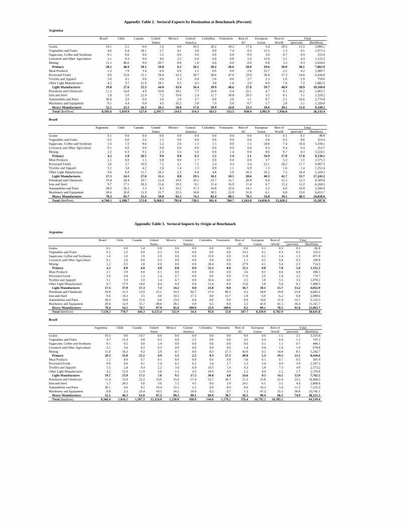
Regarding the patterns of trade, Brazil is the main destination market for Argentine exports, a trend

that has been stimulated since the formation of MERCOSUR. In 1997, Argentina’s exports to Brazil

amounted to almost a third of its total exports; and imports from Brazil had a share of around 20 percent

of the country’s total imports (see Table 2 and Table 3 in Appendix). On the other hand, Brazil’s

dependency on the Argentine market is smaller (the Argentine share in both Brazilian exports and imports

was some 10 percent). Intra-regional trade between Argentina and Brazil is highly characterized by intra-

industrial trade of manufactures, accounting for more than 70 percent of the intra-regional trade. By

product, automobiles and parts are the leading sectors (almost 30 percent), jointly with machinery and

equipment and petroleum and chemicals particularly in Brazil. There is, however, considerable

asymmetry in the structure of intra-regional trade between Argentina and Brazil. Exports of agricultural

origin (grains, processed foods and vegetables) have a substantial weight in Argentine exports, while

manufactured goods are the main products exported by Brazil. Table 3 below shows the relative sectoral

intensity of bilateral exports. A value equal to one means that the sector has the same weight in the

country’s bilateral exports that it has in the country’s total exports. The index shows that intra-regional

exports are more oriented toward heavy manufactures than are total exports in both countries; it also

shows for Brazil a small concentration on primary goods relative to the composition of its total exports.

Thus although both countries have been taking advantage of the internal market to diversified exports

towards more high valued products, this has been true particularly for Brazil.

10 During the 1990s the automotive sector has undergone a major restructuring, and specialization has been taking place among auto-part producers in MERCOSUR.For the European Union, the sectoral NTB equivalents were estimted as differences between total minus estimated protection.

<INSERT TABLE 3>

With respect to other partners, the US buys 18 percent of Brazilian exports and 9 percent of

Argentinean exports. The sectoral intensity indexes show that exports to the US are more oriented

towards heavy manufactured goods than total exports for Brazil, and more light-manufactured goods

oriented for Argentina. MERCOSUR’s purchases from the US account for 23 percent of the region’s total

imports; capital and intermediate goods are the main imports accounting for more than 85 percent of the

total imports from the US. For MERCOSUR, the EU is the most important partner. At the base year, it

accounted for 23 percent of the bloc’s total exports, and 26 percent of total imports. Biregional trade

between MERCOSUR and the EU is highly complementary. Agricultural products, including meat and

processed foods, dominate MERCOSUR’s exports to the EU market, while manufactured products,

dominated by capital goods (machinery and equipment) and intermediates (petroleum and chemicals), are

the bloc’s main imports from the EU. Compared with the sectoral intensity of exports to the US, exports

to the EU are much more oriented in primary goods (especially for Brazil). Figure 2 illustrates the

differences in MERCOSUR’s export composition to the EU and US markets. MERCOSUR’s import

composition from the EU and US is very similar: more than 85 percent are heavy manufactures and

around 8 percent light manufactures; primary imports have a share of 5 percent for imports from the US

and 1 percent for imports from the EU.

<INSERT FIGURE 2>

Regarding exports to other LAC countries, exports from Argentina are less oriented in primary goods

and more oriented towards light manufactures than total exports (except to the Chilean market). In the

case of Brazil, its exports to the LAC market are clearly oriented to high manufacture goods (see Table 3).

As we mentioned previously, the paper focuses mainly on the elimination of ad valorem tariff rates

and, to a lesser extent, the elimination of NTBs. Table 4 shows MERCOSUR’s ad valorem intra-regional

rates and the MFN rate in the base year. Almost all intra-regional trade was already liberalized and even

as sensitive a sector as automobiles still has a tariff of only around 3 percent in Argentina. The result is

that the average trade-weighted tariff for intra-bloc trade is similar and low in both countries, with very

small deviations. In contrast, the MFN tariff shows a higher average protection (trade weighted) in Brazil

(18 percent) than in Argentina (14 percent), especially in heavy manufacturing sectors. By sectors, both

countries applied the higher degree of protection to manufacturing goods.

<INSERT TABLE 4>

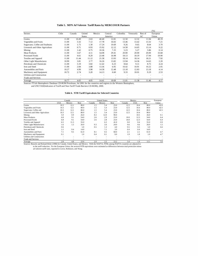
Regarding the nominal protection of MERCOSUR’s selected trade partners, the US’ highest tariffs

(11 percent) are on textiles and apparel, followed by processed foods. Chile has a moderate and uniform

protection across sectors (11 percent). Mexico is the country with the highest average protection among

the countries at the benchmark year (14 percent) and heavily protects its agricultural related industries

(grains, meat products and processed foods). While having completely liberalized intra-regional flows,

the EU heavily protects agricultural sectors by imposing MFN tariffs with rates as high as 48 percent on

sensitive goods such as grains and meats. Table 5 indicates the trade protection applied by Mercousr’s

selected partners.

<INSERT TABLE 5>

Based on the estimations made by other studies, we incorporate in the paper a tariff equivalent

quantification of the NTB for Canada, the US, Mexico and the EU. Table 6 shows the data. The most

striking characteristic is the large level of protection that the estimated NTB provides to the domestic

markets. For the United States and Canada, it goes as high as 23 percent on average for non-NAFTA

countries, while the EU has the lower average NTB protection to extra-regional partners (5 percent). The

EU protection is, however, mainly concentrated in primary goods, while manufacturing industries are

relatively little protected. In contrast, the protection faced in the US market by manufacturing exporters

can go as high as 68 percent in “automobiles and parts” and 41 percent in “textiles and apparel”. Given

the high protection level compared to the ad valorem tariffs, we anticipate big gains and large differences

in the absolute and sectoral composition results of our simulations when NTBs are eliminated.

<INSERT TABLE 6>

4. Alternative Scenarios for Policy Simulations

We simulate the formation of the two FTAs independently as well as simultaneously. Scenario 1

examines the creation of the FTAA where the countries in the Western Hemisphere eliminate all tariff

barriers to intra-hemispheric trade while keeping their individual protection structures with third partners,

namely the European Union and the rest of the world. Scenario 2 simulates the formation of a FTA

between MERCOSUR and the EU with both blocs maintaining their protection to third partners. Lastly,

scenario 3 is designed to measure the impact of creating simultaneously the FTAA and the FTA with the

European Union (EU-FTA below), with MERCOSUR serving as a hub for the two integration processes.

The countries in the Hemisphere formally launched the negotiations to create a hemispheric FTA at

the second Summit of the Americas in April 1998. In spite of the considerable skepticism regarding the

prospects of liberalizing a number of sensitive sectors, the FTAA process has steadily progressed and has

already generated significant positive impacts in a variety of areas.11 Among other things, it has

increasingly served as a catalyst for widening and deepening regional integration, supplementing the

commitment of the multilateral system to achieve a more free and open trade in the hemisphere and

beyond.

Trade talks between MERCOSUR and the EU countries started with the Interregional Framework

Cooperation Agreement, signed in December 1995, which was designed to increase economic

cooperation, enhance political dialogue and prepare for the bilateral liberalization process. At the Rio

Summit, held in June 1999, the two sides agreed to launch negotiations for the creation of an FTA

between the two blocs through a gradual and reciprocal process. Although both blocs recognize the

importance of creating an FTA, one of the most difficult challenges lies in the negotiations in agriculture,

in which MERCOSUR has a clear comparative advantage, while the EU maintains a protectionist CAP

(Common Agricultural Policy) to protect the domestic industries. This issue is increasingly dominating

the agenda of the trade negotiations, and the possibilities of deepening and balancing trade links between

the two blocs will depend greatly on the progress in this area. It is expected that the planned EU

enlargement to Eastern Europe (some of them being big agricultural producers) will alter the EU’s trade

policy on agriculture.

An important aspect of the MERCOSUR-EU relationship is that in light of the growing US trade

dominance and the ongoing hemispheric negotiations, MERCOSUR views the EU as a counterbalance to

the US, particularly in the FTAA negotiation process. For the EU, MERCOSUR is an important extra-

regional trade partner: it absorbs some 50 percent of its exports to Latin America, and represents half of

total exports from Latin America to the EU market. From the EU perspective, MERCOSUR has been a

traditional stronghold in the Americas, and is now increasingly important partner to block US dominance

and to restore the lost share in Latin America by strengthening trade relations and promoting business

opportunities. Since the EU and the US are competitors in the South American market, this is a very

important parallel agenda to the FTAA.

11 See Integration and Trade in the Americas, Periodic Note, IDB, Department of Integration and Regional Programs, several issues.

The paper uses two policy instruments: ad valorem tariff protection and non-tariff barriers (NTBs). It

is widely acknowledged that, in addition to tariff protection, NTBs are crucial elements in the trade

liberalization negotiations for developing countries, and without their elimination it will not be possible to

realize all the processes’ benefits. This is particularly true today, given that the levels of nominal

protection on trade flows have become fairly low in the Western Hemisphere and in the European Union.

Table 7 summarizes the alternative scenarios. Simulations under Experiment A consider only the

elimination of the ad valorem tariff barriers, while simulations under Experiment B include the complete

elimination of the NTBs in addition to tariffs. In each case we assume the IRTS version of the model. We

also simulate a CRTS version of the economies (Version A) and use the simulation results under

Experiment A (tariff only) and Version A (CRTS) as the base experiment in evaluating the effects of the

NTBs and scale economies.

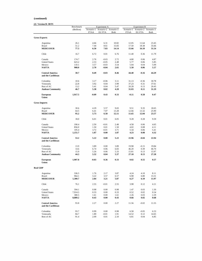
<INSERT TABLE 7>

5. Simulation Results

5.1. Aggregate Results

In this section, we evaluate the aggregate impact on MERCOSUR countries of the three integration

scenarios analyzed in the paper. The aggregate effects are examined by focusing on the absolute

increment and rate of growth of exports and imports, as well as on the rate of growth of real GDP.

As expected, the results reveal that regional integration generates considerable gains for all countries

in the agreement, substantial changes in trade patterns, and structural adjustment in domestic production.

Overall exports to intra- and extra-hemispheric markets grow for Argentina and Brazil as efficiency gains

and global competitiveness increase. Guaranteed access to large markets, enabling firms to exploit

economies of scale, and the dynamic externality effects resulting from the trade liberalization enhance the

gains. Table 4 in the Appendix shows the aggregate results for all scenarios and regions in the model.

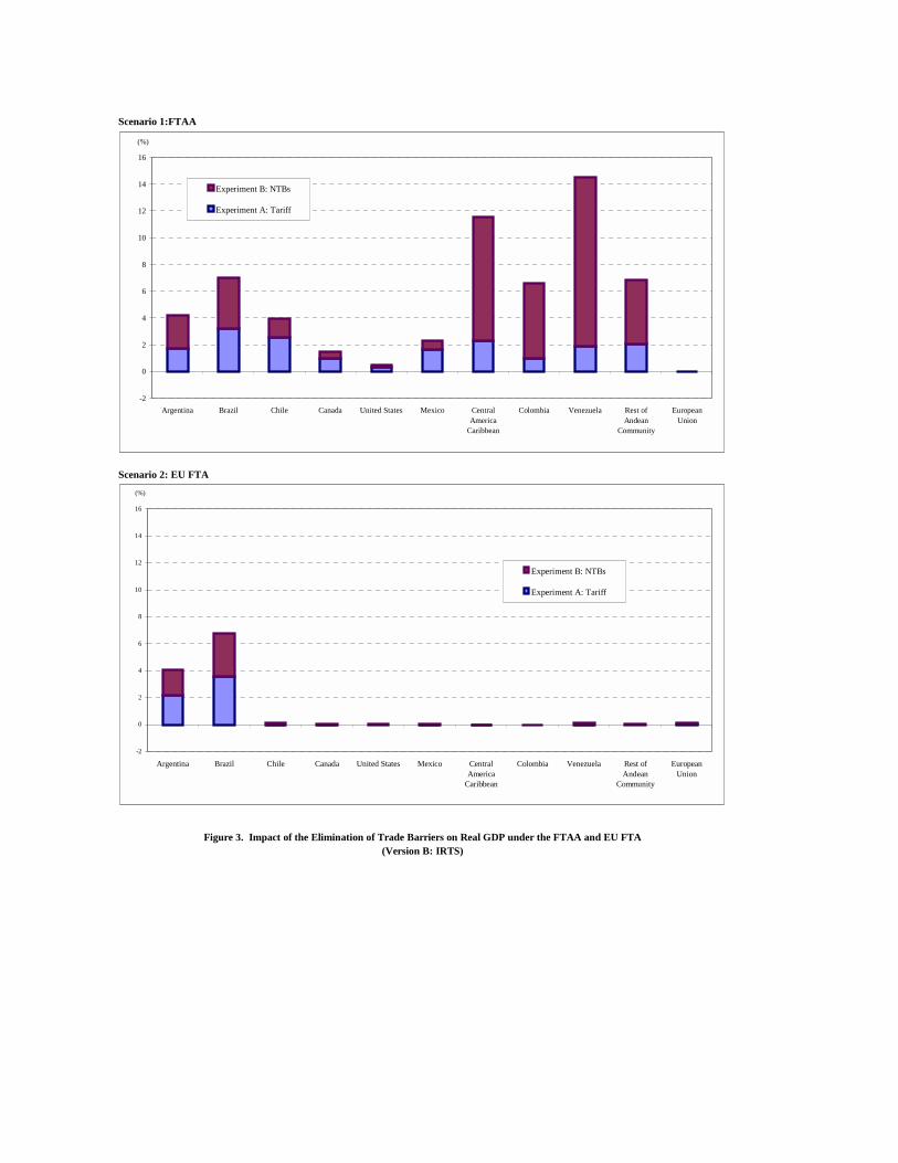
Figure 3 next shows the real GDP effects in the IRTS case for the FTAA and EU-FTA scenarios

(scenarios 1 and 2).

<INSERT FIGURE 3>

In the presence of IRTS and tariff-only elimination, FTAA induces export growth by 4.7 percent in

Argentina and 7.4 percent in Brazil. Exports destined to the US are up by 7.4 percent in Argentina and 9

percent in Brazil. Due to the relatively high initial protection and low base exports, exports to Central

America and the Caribbean as well as to the Andean Community see a substantial increase of 15 percent.

For these countries, export growth under FTAA is 8.5 percent in Central America and the Caribbean and

5.4 percent in the Andean Community; the expansion of exports in the NAFTA countries is smaller than

in other hemispheric partners due to a market which was already highly liberalized at the benchmark. The

EU excluded from the agreement faces trade diversion in the MERCOSUR market as imports from

the EU decrease by 2.5 percent and 3.2 percent in Argentina and Brazil, respectively (mainly heavy

manufactures). Imports from the Rest of the World also decrease by more than 3 percent.

For MERCOSUR, integration with the European Union generates a greater impact on export

performance than the FTAA, as exports grow an additional 1.4 percentage point. In addition to the 27

percent and 16 growth in exports to the EU from Argentina and Brazil, respectively, exports to extra-

agreement countries also increase (thus translating the increased efficiency into an overall increase in

other countries’ import market share). The EU-FTA is also likely to create negative trade effects on

countries left outside the agreement: imports of light and heavy manufacturing products from non-EU

countries are displaced in the MERCOSUR market (although imports of primary goods increase).

The simultaneous arrangement scenario (scenario 3) generates important gains for MERCOSUR. It

doubles the bloc’s aggregate trade and GDP gains when compared to the FTAA, and increases it by as

much as 80 percent compared to the EU-FTA. The growth of exports from other non-members in the

Western Hemisphere remains virtually unchanged from the level of gains realized in the FTAA-only

scenario. Left outside of the agreement, MERCOSUR’s imports from the Rest of the World decrease by

around 4 percent.

The inclusion of NTBs in the liberalization process (Experiment B) further expands exports in all

countries. MERCOSUR’s aggregate export growth more than doubles from the tariff-only simulation (15

percent growth or more in the first two scenarios and more than 30 percent growth in the simultaneous

arrangement). The gains of eliminating the NTBs are slightly greater for Argentina than for Brazil in

terms of additional real GDP and export growth from the tariff-only scenario. In the FTAA case,

MERCOSUR’s exports to all countries further increase from the tariff-only experiment favored by the

increased demand in Hemispheric partners that benefit from the removal of the NTBs by NAFTA

members, especially on key exports that faced high NTBs in the US. In fact, export growth is now more

than five times higher than it is shown to be under the tariff-only simulation for Central America and the

Caribbean, Colombia and Venezuela. A main difference from the tariff-only experiment is that we do not

observe trade diversion effects in the MERCOSUR market. Given the balanced trade assumption as well

as technology and resources constraints in each region, intra-hemispheric export supply cannot meet the

increased demand in the hemisphere. As a result, countries expand imports also from extra-hemispheric

sources.12 Although, to a lesser extent, the same happens in the EU-FTA scenario.

The impact on welfare measured in real GDP is highly correlated with trade performance. Under the

tariff-only experiment, FTAA induces a growth in MERCOSUR’s real GDP of 2.8 percent (followed by

Chile, 2.5 percent, and Central America and the Caribbean, 2.3 percent). MERCOSUR’s gains from

integration with the European Union (scenario 2) are greater than under the FTAA, and real GDP in

MERCOSUR grows now by 3.2 percent. MERCOSUR greatly benefits from the cross-fertilization effects

of the simultaneous integration (scenario 3), which nearly doubles the real GDP growth from the FTAA

and is 80 percent greater than in the integration with the European Union.

The additional elimination of the NTBs (Experiment B) further enhances real GDP growth, although

the results vary considerably by country. FTAA now increases MERCOSUR’s GDP by 6 percent from

the benchmark, more than twice the growth under the tariff-only elimination (Experiment A). The

Andean Community (especially Venezuela and Colombia) as well as Central America and the Caribbean

are again the largest beneficiaries from the FTAA. Compared to the tariff-only simulation results, the

EU’s removal of NTBs in scenario 2, mostly in agriculture, increases GDP for MERCOSUR by an

additional 90 percent, and the simultaneous arrangement (scenario 3) by nearly an additional 100 percent.

An interesting point to make is that the introduction of NTBs as a policy variable makes the FTAA a

better option for MERCOSUR countries than the EU-FTA, thus reversing the ranking from the tariff-only

scenario. An explanation for this is the fact that NTBs in the EU are concentrated in agriculture industries,

while NTBs in the NAFTA countries are also high in key manufacturing sectors such as, inter alia,

automobiles and textiles. Therefore, the additional impact of trade liberalization on manufacturing

industries would be greater in the FTAA than in the EU-FTA case (and remember that the highest

productivity gains of trade liberalization will be in the manufacturing industries).

Compared to the CRTS case (Version A), the IRTS engenders an additional increase in export and

real GDP growth, the extent of which depends on the degree of realization of economies of scale during

12 This is, however, not the case with NAFTA members. Due to the elimination of high protection to intra-hemispheric imports only (thus maintaining it against third parties), we observe strong trade diversion effects.

the adjustment process. As the number of firms in each industry is fixed, firms reduce their average costs

as the industry expands outputs, lowering prices accordingly. Therefore, efficiency varies with total

sectoral output. In particular, the presence of economies of scale induces an additional increase in total

production, although the results by sector vary according to the degree of unrealized economies of scale

in each country (see next section).

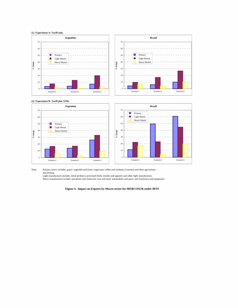
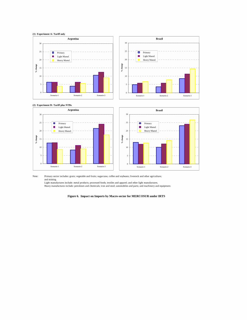
5.2 Sectoral Results

As in the previous section, we focus on the IRTS scenario and use the CRTS scenario as a reference

point. To facilitate the analysis, we aggregate the 13 sectors into three macro-sectors: primary, light and

heavy manufactures.13 Figures 4 and 6 present the impact on exports and imports growth from the

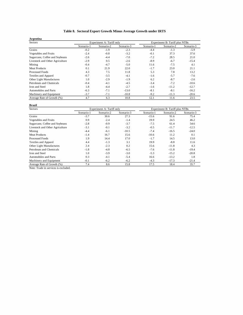
benchmark, Figure 5 shows the macro-sector composition of the increased exports and Table 8 the

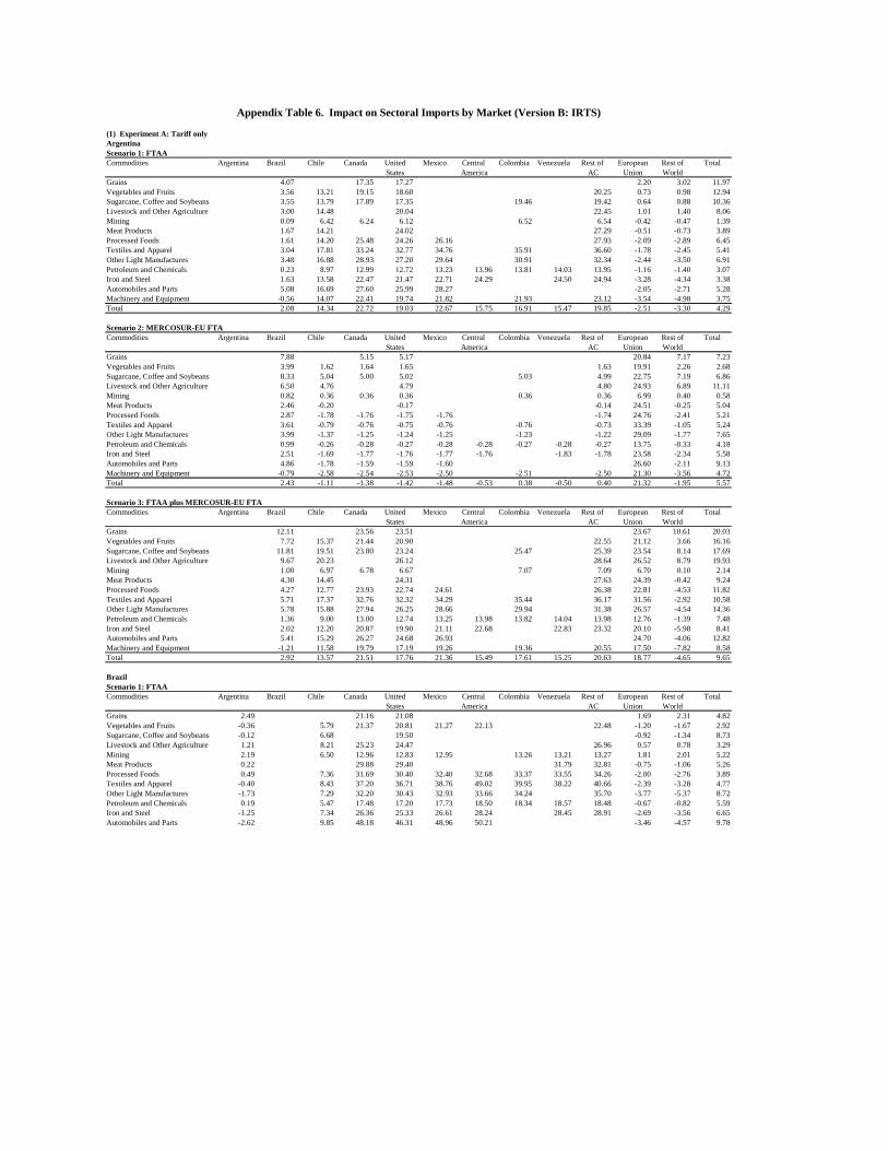
sectoral export growth differences. Tables 5 and 6 in the Appendix shows a more detailed sectoral impact

on exports and imports by market.

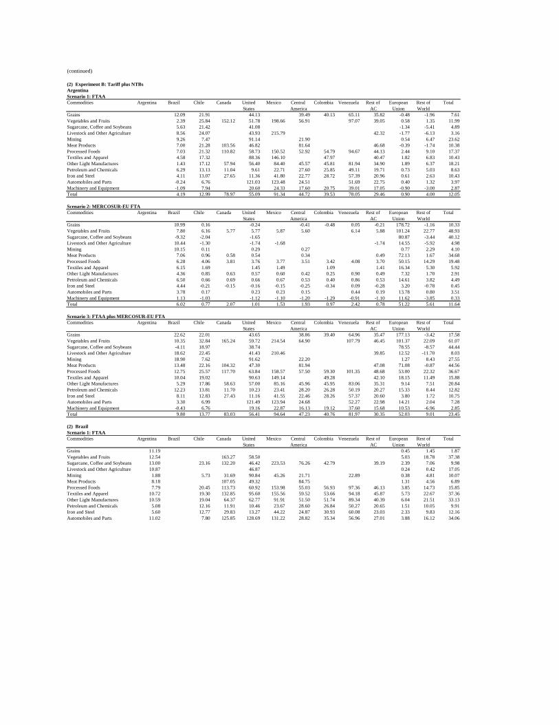
(1) Tariff-only elimination

The light-manufacturing sector experiences the highest export growth across the macro-sectors. It

grows by more than 12 percent under the EU-FTA scenario and by around 10 percent under the FTAA

formation.

In terms of products or sectors, the EU-FTA generates a more heterogeneous export growth across

sectors than the FTAA, which presents smaller growth differences across sectors (see Table 8). Under the

EU-FTA, the sectors in Argentina which exhibit more dynamic growth are “meat products” (growing 22

percentage points above the average growth) followed by “processed foods” (7.5 percentage points above

average), while Brazil’s are “meat products” and “processed foods”(growing 15 percentage points above

the average). 14 In fact, agricultural related exports (raw products and agro-products) constitute 87 percent

of the increased exports to the European Union, and meat products and processed foods alone account for

approximately half of those exports. Under FTAA Argentina’s most dynamic sector is “processed foods”

(grows 4.3 percentage points above the average growth), while Brazil’s is “textiles and apparel” (4.4

percentage points above the average).

13 Primary sectors include: grains; vegetables and fruits; sugarcane, coffee and soybeans; livestock and other agriculture; and gas and oil. Light manufactures include: meat products; processed foods; textiles and apparel; and other light manufactures. Heavy manufactures include: petroleum and chemicals; iron and steel; automobiles and parts; and machinery and equipment. 14 An interesting case is the “grain” sector in Brazil that grows 30 percentage points above the average. This is due primarily to the small value of exports in the base year and the EU’s highest initial MFN tariff (48 percent) on this sector.

An important difference between the two scenarios is that FTAA brings a stronger export growth in

the heavy manufacturing sectors than the EU-FTAA, particularly in Brazil. In value terms, heavy

manufactured exports in the FTAA case account for nearly half of the increased exports in Brazil, and

around 15 percent in Argentina; in the EU-FTA case the share is slightly over 20 percent and 5 percent in

Brazil and Argentina, respectively. In contrast with these figures, agricultural related exports (raw

products and agro-products) constitute 87 percent of the increased exports to the European Union, and

meat products and processed foods alone account for approximately half of those exports destined to the

EU market.

Thus the Hemispheric integration scheme promotes exports with higher value-added than integration

with the European market. This result is due to the differences in export composition between the

Hemispheric and European markets in the base-year, together with the initial highly protected European

market for agricultural goods (primary and agro-products, such as meat and processed goods). It is

important to note, however, that in relative terms exports to Latin-American partners in the FTAA

agreement are more valued-added exports than exports to the US market (especially for Brazil). Also

interesting is the fact that Argentina’s exports of heavy manufactures to the Brazilian market suffer a

decrease in both scenarios, as they are displaced by more efficient producers in the Hemisphere, in one

case, and more efficient European producers, in the other. For Brazil, intra-regional exports decrease only

in the “machinery and equipment” sector.

The impact on imports growth is more balanced than it is for exports (Figure 6). In value terms,

however, heavy manufactured goods, typified by intermediate (petroleum and chemicals, and iron and

steel) and capital goods (machinery and equipment) account for more than three-quarters of the increased

imports in both the FTAA and EU-FTA scenarios. In the EU-FTA case it accounts for nearly 90 percent

of the manufactured imports.

MERCOSUR countries undergo a substantial adjustment in production. The aggregated income

effects of the FTAA and EU-FTA formations induce an expansion in production in all sectors (except

machinery in Argentina). Production capacity expands more rapidly in the primary and light

manufactures industries, the latter presenting a strong export orientation.15 Given the fixed resource

constraint, these adjustments in production effect a reallocation of domestic resources (labor and capital).

Labor and capital thus move away from manufacturing industries (especially from heavy industries such

as machinery and equipment) into agriculture. Manufactures experience the highest productivity increase

from the trade liberalization, and thus increase output while decreasing factors demands (especially light

manufactures), while labor-intensive primary goods absorb factors, mainly labor.

The results of the scenario involving the simultaneous FTAs (scenario 3) lie between those of the two

individual arrangements. Light manufactures lead the bloc’s export growth (20 percent in Argentina and

27 percent in Brazil). Processed foods account for nearly half of the increased exports in Argentina and

for one-third in Brazil. Exports of heavy manufactures grow at a slow pace (2.7 percent) in Argentina, but

show a marked increase (of 10 percent) in Brazil. Heavy manufactured goods account for approximately

one-third of the new exports in Brazil. The booming economy forces domestic industries to undergo an

even bigger structural adjustment in the production and factor markets. As in the other two scenarios,

production capacity expands more rapidly in agriculture and light manufacturing industries than in heavy

industries. Processed foods undergo the largest production increase 12 percent in Brazil and 8.5 percent

in Argentina.

Compared to the CRTS case, we note that the benefits of the realization of economies of scale in

manufactures spill over to other sectors as we see further growth in output across all industries. Moreover,

the additional gains are evenly distributed across sectors. This should not come as a surprise since

MERCOSUR countries are not the only countries that can benefit from the potential realization of

economies of scale in manufactures.

(2) Tariffs plus NTBs elimination

In the FTAA case, the elimination by the US of NTBs on highly protected domestic industries —

mining, textiles and apparel, other light manufactures and automobiles—produces a strong additional

export growth in almost all sectors, but especially in those mentioned above. There are big differences in

the sectoral or product composition of exports compared to the tariff-only case (see Table 8); however,

we observe a similar pattern at the macro-sector level: light manufactures lead export growth in both

countries, while heavy manufactures account for around 35 percent of the increased exports in Brazil. The

bloc’s exports to the US jump to 55 percent in Argentina a 45 percent in Brazil (7.4 and 5 times the

growth under the tariff-only experiment); but exports to the other NAFTA countries also increase by more

than 60 percent (in fact, Argentinean exports to the Mexican market growth by 100 percent). In the EU- 15 In general, we observe a relative export specialization --an increase in the ratio exports over production, d(E/X)/(E/X)-- in manufacturing industries, especially in Brazil due to the high export growth in heavy

FTA scenario, the gains of eliminating NTBs are very concentrated in agriculture. Primary goods exports

increase by more than 12 percent and almost 50 percent in Argentina and Brazil, respectively, a large

change compared to the growth rate in the tariff-only scenario of around 5 percent. Both countries

become much more primary goods exports oriented (especially Brazil). Aggregate exports to the EU jump

by 50 percent, more than twice the export growth under the tariff-only experiment. Agricultural exports

account for more than 90 percent of the increased exports to the European Union.

Compared with the tariff-only experiment, the MERCOSUR countries –and especially Brazil—

greatly expand automobile production, demanded primarily by the United States after eliminating the

high NTBs in the industry. The same happens in Argentina with the mining sector. In the EU-FTA case,

primary industries with a high NTB protection (grain, vegetables and fruits, and sugar, coffee and

soybeans) experience higher additional output growth. As a consequence, domestic resources are driven

away from heavy industries into primary industries. In fact, in the simultaneous agreement scenario,

around seven percent of labor and capital are pulled from machinery and equipment industries, which

grow the most slowly in Brazil, and even shrink by 2.7 percent in Argentina. Since the primary sectors are

characterized by low efficiency relative to manufacturing industries, the resource pull in the former

sectors is larger in the EU-FTA than in the FTAA scenario.

Given that the additional manufacturing industries’ output growth is larger under the FTAA than

under the FTA-EU (the industries with the higher productivity arising from trade externalities and scale

economies), the additional overall growth from eliminating the NTBs is greater in the FTAA than in the

EU-FTA scenario.

6. Summary and Conclusions

Regional integration is not simply a process of maximizing potential economic gains, but rather a

strategic process that also involves political elements concerning the adjustment costs arising from

structural reforms and transformation (particularly labor market adjustment and industrial lobbying from

the sensitive sectors). As is the case for many other countries in Latin America, the members of

MERCOSUR have an active regional integration agenda that includes the FTAA and an FTA with the

EU, the two broadest agreements under negotiation.

Applying a multi-region, multi-sector general equilibrium model incorporating trade-linked

manufacturing.

externalities and scale economies in manufacturing industries, this study examines the potential economic

gains and structural adjustment of the two FTAs under negotiation (individually and simultaneously

considered). The integration options are evaluated by eliminating the ad valorem tariffs only and also by

eliminating simultaneously NTBs for selected countries.

The simulation results show the FTAA and the MERCOSUR-EU FTA generate substantial economic

gains for the two MERCOSUR countries. When only tariffs are eliminated, we observe that the FTAA

option is slightly inferior to the FTA with the EU (although the opposite is true when NTBs are also

eliminated). Hemispheric integration greatly stimulates export specialization in manufacturing industries

relative to the primary sector (this impact being stronger in Brazil than in Argentina). Latin American

countries greatly contribute to this result since exports of MERCOSUR to these countries have a higher

valued-added content than exports to the North-American neighbors. Policy makers should be aware of

the importance of reinforcing the trade links with other Latin American countries as a means to increase

the valued content of exports. On the other hand, mainly due to the EU’s initially high tariff protection in

agriculture, integration with the EU largely expands agricultural exports, in which MERCOSUR has a

clear comparative advantage and competitiveness in global markets. The simultaneous approach (that

generates dynamic cross-fertilization effects) almost doubles the gains from the individual FTAs. The

bloc expands manufactured exports to the hemispheric market, and agricultural exports to the European

Union, while heavily concentrating on imports of capital and intermediate goods from both sources.

Although, when compared to tariffs, the measurement of NTBs is imperfect and less accurate, the

results show how important the inclusion of NTBs in the negotiation can be for MERCOSUR, as well as

for other Latin American countries. When considering the elimination of NTBs, the gains in trade and

GDP growth are twice that of the benefits which accrued from only the elimination of tariffs and, given

the model’s assumption regarding resource constraints, also limits the amount of trade diverted from

partners outside the agreement relative to that which is observed when only tariffs are eliminated.

The increase in industry outputs is largely met by the efficiency gains arising from trade-linked

externalities and scale economies. The results showing that output grows after liberalization in all sectors

(except machinery in Argentina) should be read with caution. The substantial adjustment in production

induces a strong adjustment in factor markets as domestic resources are reallocated from manufacturing

or contracting industries into the primary sectors freely and costlessly, not taking into consideration that

the reallocation of labor has considerable social and political costs (nor accounting for factor market

rigidities).

MERCOSUR faces a difficult moment in its drive toward trade liberalization and regional economic

integration; a moment made especially crucial by its prolonged internal economic instabilities. In the

meantime, the group will confront a busy timetable on its external agenda in the coming years, which

requires crucial decision-making. While being a formidable challenge, it may also offer an excellent

opportunity for the bloc to harmonize internal and external policies, to identify common grounds and

interests, and to raise global credibility and competitiveness.

REFERENCES

Behar, J., (1995) “Measuring the Effects of Economic Integration for the Southern Cone Countries:

Industry Simulations of Trade Liberalization,” Developing Economics, 33(1), 4-31. Brown, D.K, A.V. Deardorff, and R.M. Stern (1995) “Expanding NAFTA: Economic Effects of

Accession of Chile and Other Major South American Nations,” North American Journal of Economics and Finance, 6(2), 149-170.

_______ (1998) Computational Analysis of the Accession of Chile to the NAFTA and Western

Hemispheric Integration, Research Seminar in International Economics, Discussion Paper No. 432, Ann Arbor, University of Michigan.

Bussolo, M. and D. Roland-Holst (1998) Columbia and the NAFTA, Working Paper Series, Paris, OECD

Development Center. Connolly, M. and J. Gunter (1999) “MERCOSUR: Implications for Growth in Member Countries,”

Current Issues in Economics and Finance, 5 (3) Federal Reserve Bank of New York. Cox, D. and R. Harris (1985) “Trade Liberalization and Industrial Organization: Some Estimates for

Canada,” Journal of Political Economy 93(1), 115-145. Devlin, R. and R. Ffrench-Davis (1999) “Towards an Evaluation of Regional Integration in Latin

America in the 1990s,” World Economy, 22 (2), March. Diao, X., and A. Somwaru (2000) “An Inquiry on General Equilibrium Effects of MERCOSUR-An

Intertemporal World Model,” Journal of Policy Modeling, 22 (5), 557-588. ___________, (2001) “A Dynamic Evaluation of the Effects of A Free Trade Area of the Americas-An

Intertemporal, Global General Equilibrium Model,” Journal of Economic Integration, 22 (5), 557-588.

Dias, V.V. M. Cabeza and J. Contador (1988) “Trade Reforms and Trade Patterns in Latin America,”

Paper presented at the IV Conference of the Latin and Caribbean Economics Association (LACEA), Santiago, Chile.

Fernandez, R. (1997) “Returns to Regionalism: An Evaluation of Non-Traditional Gains from RTAs,”

Paper presented under the auspices of the World Bank International Trade Division Programs on Regionalism and Development.

Giambiay, Fabio (1999): “MERCOSUR: Why Does Monetary Union Make Sense in the Long Term?,”

Integration and Trade, v.3, Inter-American Development Bank, September/December 1999. Giordano, P. and M. Watanuki (2000): “Economic Effects of a MERCOSUR-European Communities

Free Trade Agreement: A Computable General Equilibrium Analysis,” in Paolo Giordano, Alfredo Valladao and Marie Francoise (eds.), Toward an agreement between Europe and the Mercosur, Paris: Presses de Sciences Po (forthcoming).

Gunasekera, H.D.B.H. (1991) Imperfect Competition and Returns to Scale in a Newly Industrializing Economy: A General Equilibrium Analysis of Korean Trade Policy,” Journal of Development Economics 34, 223-247.

Francois, J.F. and D. Roland-Holst (1997) “Scale Economies and Imperfect Competition,” in J.F.

Francois and K.A. Reinert (eds.,) Applied Methods for Trade Policy Analysis: A Handbook, Cambridge University Press: New York.

Flores, R.G.Jr. (1997) “The Gains from MERCOSUL: A General Equilibrium Imperfect Competition

Evaluation,” Journal of Policy Modeling, 19(1), 1-18. Gray, D., B. Ksissoff and M. Tsigas (1996) Western Hemisphere Integration: Trade Policy Reform and

Environmental Policy Harmonization, Presented at the Symposium sponsored by the International Agricultural Trade Research Consortium and Inter-American Institute for Cooperation on Agriculture.

Harris, R. (1984) “Applied General Equilibrium Analysis of Small Open Economies with Scale

Economies and Imperfect Competition,” American Economic Journal 74(5), 1016-1032. Harrison, G. W., T. F. Rutherford and D. G. Tarr (1994) Product Standards, Imperfect Competition and

Completion of the Market in the European Union, Policy Research Working Paper 1293, World Bank, Washington D.C.

Harrison, G. W., T. F. Rutherford and D. G. Tarr (1997) “Trade Policy Options for Chile: A Quantitative

Evaluation,” Policy Research Working Paper 1783, World Bank, Washington D.C. Hertel, T.W. (1997) Global Trade Analysis: Modeling and Applications, New York: Cambridge

University Press.

Hinojosa-Ojeda, R.A., J.D. Lewis and S. Robinson (1995) “Regional Integration Options for Cental America and the Caribbean’s after NAFTA,” North American Journal of Economics & Finance, 6(2), 121-148.

___________, (1997) Convergence and Divergence between NAFTA, Chile, and MERCOSUR: Dilemmas

of North and South American Economic Integration, Working Papers Series 219, Inter-American Development Bank, Washington D.C.

Hoekman, B. M. Schuff and A. (1998) “Regionalism and Development: Main Message from Recent

World Bank Research,” Development Research Group, World Bank, Washington, D.C. IMF, (1997) Government Finance Statistics Yearbook, IMF, Washington, D.C. ___________, (1998) Direction of Trade Statistics Yearbook, IMF, Washington, D.C. Inter-American Development Bank (IDB), (1996), “Trade Liberalization,” in Economic and Social

Progress in Latin America, Chapter 2, Inter-American Development Bank, Washington, D.C. ___________, MERCOSUR: INTAL MERCOSUR, Various Reports, IDB/INT, Washington, D.C. ___________, Integration and Trade in the Americas, Periodic Note, IDB/INT, Various Issues,

Washington, D.C.

International Labor Office (ILO), (1997) Yearbook of Labor Statistics, ILO, Geneva. Lewis, J.D., S. Robinson, and Z. Wang (1995) Beyond the Uruguay Round; the Implications of an Asian

Free Trade Area, Policy Research Working Paper 1467, World Bank, Washington, D.C. Luna, S. A. (1997) “The Response of Mexican Manufactures to Trade Liberalization: Results from a

Computable General Equilibrium Analysis,” paper presented for the Conference on Mexico-Caribbean Trade Relations, Port of Spain, and Trinidad and Tobago.

Melo, J. de. and D. Roland-Holst (1991) “An Evaluation of Neutral Trade Policy Incentives Under

Increasing Returns to Scale,” J. de Melo and A. Sapir (eds.,) Trade Theory and Economic Return: North, South, and East, Basil Blackwell: Cambridge, MA.

________ and S. Robinson (1992) “Productivity and Externalities: Models of Export-led Growth,”

Journal of International Trade and Economic Development, 1, 41-69. ________ and D. Tarr (1992) A General Equilibrium Analysis of US Foreign Trade Policy, MIT Press:

Cambridge: MA. Milner, C. and P. Wright (1998) “Modeling Labor Market Adjustment to Trade Liberalization in an

Industrializing Economy,” Economic Journal, 108, 509-528. Moreira, M.M. and S. Najberg (2000) “Trade Liberalization in Brazil: Creating or Exporting Jobs?,”

Journal of Development Studies, 36(3), 78-99. Nagarajan, N. (1998) MERCOSUR and Trade Diversion: What Do the Import Figure Tell Us? Economic

Paper No 129, European Commission, Brussels, Belgium. Norman, V.D. (1990) “Assessing Trade and Welfare Effects of Trade Liberalization: A Comparison of

Alternative Approaches to CGE Modeling with Imperfect Competition,” European Economic Review 34, 725-751.

Olarreaga, M. and I. Soloaga (1996) “Explaining Mercosur Tariff Structure: A Political Economic

Approach,” paper as a part of the World Bank International Economic Division Research Program on Regionalism, October.

________, I. Soloaga and A. Winters (1999) “What behind Mercosur’s CET?” paper presented at the

development research trade workshop, World Bank, Washington, D.C. Reinert, K.A., and D.W. Roland-Holst (1992) “Armington Elasticities for United States Manufacturing

Sectors,” Journal of Policy Modeling, 14 (5). 631-639. Robinson, S., M.E. Burfisher, R. Hinajosa-Ojeda, and K.E. Thierfelder (1993) “Agricultural Policies and

Migration in a U.S.-Mexico Free Trade Area: A Computalbe General Equilibrium Analysis,” Journal of Policy Modeling, 15(5&6), 673-701.

Roberts, J.M. (2001) Estimates of the Productivity Trend Using Time-Varying Parameter Technique,

Board of Governors of the Federal Reserve System.

________, and K. Thierfelder (1999) Trade Liberalization and Regional Integration: The Search for Large Numbers, TMD Discussion Paper 34, International Food Policy Research Institute, Washington, D.C.

Rodrik, D. (1988) “ Imperfect Competition, Scale Economies, and Trade Policy in Developing

Countries,” R.E. Baldwin (ed.) Trade Policy Issues and Empirical Analysis, University of Chicago Press: Chicago.

Roland-Holst, D.W., K.A. Reinert and C.R. Shiells, (1994) “A General Equilibrium Analysis of North

American Integration,” in F.J. Francois and C.R. Shiells (eds.), Modeling Trade Policy: Applied General Equilibrium Assessments of North American Free Trade, Cambridge University Press.

Stiroh, K.J. (2001) Information Technology and the U.S. Productivity Revival: What Do the Industrial

Data Say?, Federal Reserve Bank of New York. US International Trade Commission (1997) The Dynamic Effects of Trade Liberalization: An Empirical

Analysis, USITC Publication 3069, USITC, Washington, D.C. Teixeira, E.C. and S.R. Valverde (2000) Impact of MERCOSUL, AFTA, and WTO Round Agreements on

the Economies of Argentina, Brazil and Chile, Paper presented at the Third Annula Conference on the Global Economic Analysis (Melbourne, Australia) in June 2000.

Winters, L.A. (1996) “Regionalism and Multilateralism,” Policy Research Working Paper 1687, World

Bank, Washington, D.C. World Bank, (1998) World Development Report 1997, World Bank, Washington, D.C. Wonnacott, P., and R.J. Wonnacott (1995) “Liberalization in the Western Hemisphere: New Challenges

in the Design of a Free Trade Agreement,” North American Journal of Economics & Finance, 6(2), 107-119.

Items Description

1. Production Sectors All regions produce 15 goods using primary inputs and intermediategoods with a CES production technology. The 15 sectors in ROWare fully endozenized. Version A assumes CRTS across the sectors,while version B assumes IRTS for the manufacturing industries.

2. Market Structure Version A applies perfect competition for all sectors. In version B,each of the manufacturing industries faces contestable market, andother sectors are in perfect competition in their respective markets.

3. Demand Final demand in each country or region is derived from household'sutility maximizing behavior subject to budget constraint. Intermediatedemands are determined by the fixed proportion of the input-outputcoefficients.

4. Trade Exports are specified by a CET function, and differentiated by marketof destination and from domestic supply. Imports are modeled with a CES specification, and differentiated by market of origin.

5. Factors(i) Land Sectorally fixed, and only used in agriculture.(ii) Capital Sectorally mobile, but immobile internationally. Total supply in each

country or region is fixed.(iii) Labor Same as capital.

6. Trade-linked Externalities(i) Sectoral export externality(ii) Import externality of intermediate inputs and capital goods(iii) Aggregate export externality

7. Major Assumptions(i) Saving-Investment Identity: Current amount of savings are fully utilized for investment.(ii) Balanced Trade: Trade remains balanced for each country and region. In other words,

initial balance of trade in goods and services remains constant.(iii) Balanced Budget: Government balances revenues and expenditures including exogenous

foreign transactions.(iv) Small Country: No country has market power to influence world prices through trade,

and each country behaves as a price taker.(v) No Financial Market: The model deals with the real side of the economy.

Note: CET means Constant Elasticity of Transformation, and CES is Constant Elasticity of Substitution. CRTS and ITRS are Constant Return to Scale and Increasing Returns to Scale, respectively.

Table 1. Main Features and Assumptions of the MERCOSUR CGE Model

Sectors Countries/regions

Primary Sectors ArgentinaGrains BrazilVegetables and Fruits ChileSugarcane, Coffee and Soybeans CanadaLivestock and Other Agriculture United StatesMining Mexico

Central America and the CaribbeanLight Manufactures Colombia

Meat Products VenezuelaProcessed Foods Rest of the Andean CommunityTextiles and Apparel European Union Other Light Manufactures Rest of the World (ROW)

Heavy ManufacturesPetroleum and ChemicalsIron and SteelAutomobiles and PartsMachinery and Equipment

ServicesUtilities and ConstructionTrade and Services

Table 2. Sectors and Regions in the MERCOSUR CGE Model

ArgentinaBrazil Chile Canada United Mexico Central Colombia Venezuela Rest of European Rest of

States America AC Union WorldGrains 0.88 0.44 0.00 0.09 0.00 1.78 1.76 1.67 1.52 0.29 1.78Vegetables and Fruits 1.12 0.10 4.43 0.65 0.99 0.94 0.00 1.80 0.12 2.80 0.32Sugarcane, Coffee and Soybeans 0.14 0.66 0.00 1.64 0.00 0.00 0.00 0.00 0.00 3.38 0.84Livestock and Other Agriculture 0.49 0.07 0.00 0.94 0.50 0.00 0.00 0.00 0.23 2.57 1.19Mining 1.19 4.35 0.00 2.22 0.00 0.19 0.00 0.00 0.00 0.09 0.35 Primary 0.93 1.56 0.60 0.99 0.21 0.87 0.67 0.88 0.63 0.98 1.03Meat Products 0.28 1.88 0.83 1.44 0.00 0.27 0.00 0.00 0.62 3.05 0.53Processed Foods 0.36 0.49 0.86 0.79 1.35 2.06 1.24 1.91 0.81 1.49 1.52Textiles and Apparel 1.92 1.42 0.00 0.20 1.14 0.00 1.91 0.00 0.93 0.45 0.54Other Light Manufactures 0.58 0.51 4.30 2.51 0.91 0.63 0.52 0.22 0.37 1.24 1.09 Light Manufactures 0.51 0.71 1.43 1.13 1.11 1.45 1.03 1.25 0.71 1.53 1.26Petroleum and Chemicals 1.10 1.38 0.48 1.06 1.77 0.76 2.03 0.63 2.46 0.47 0.89Iron and Steel 0.35 0.99 4.21 1.42 3.85 0.48 2.30 2.13 4.03 0.68 1.21Automobiles and Parts 2.82 0.19 0.00 0.34 0.27 0.34 0.00 0.18 0.10 0.07 0.20Machinery and Equipment 1.79 0.87 0.00 0.88 2.01 0.74 1.46 1.10 1.31 0.33 0.55 Heavy Manufactures 1.68 0.82 0.85 0.84 1.64 0.57 1.29 0.80 1.72 0.34 0.65

BrazilArgentina Chile Canada United Mexico Central Colombia Venezuela Rest of European Rest of

States America AC Union WorldGRAIN 0.76 0.00 0.00 0.00 0.00 0.00 0.00 0.00 0.00 2.02 1.15VEGET 0.37 0.00 3.99 2.46 0.00 0.00 0.00 0.00 0.00 1.37 0.28OTHAG 0.15 0.15 0.82 0.50 0.24 0.12 0.15 0.00 0.10 2.38 0.71LIVES 0.27 0.00 0.00 1.94 0.00 0.00 0.00 0.00 0.00 1.20 0.95MINING 0.35 0.05 1.51 0.37 0.87 0.80 0.00 0.23 0.00 1.37 1.54 Primary 0.24 0.10 1.15 0.55 0.45 0.35 0.09 0.08 0.06 1.96 1.00MEATP 0.69 0.00 0.37 0.25 0.00 0.57 0.00 0.00 0.00 1.20 1.73PFOOD 0.20 0.21 0.56 0.42 0.29 0.40 0.13 0.25 0.19 1.41 1.59TXTIL 2.13 1.57 1.73 1.05 0.57 0.92 3.65 0.43 2.82 0.54 0.66OTLMF 0.64 0.67 1.12 1.95 0.22 0.80 0.46 0.49 0.99 0.98 0.72 Light Manufactures 0.52 0.43 0.80 0.92 0.26 0.58 0.48 0.31 0.61 1.20 1.27PETRO 1.58 1.65 0.87 1.09 1.54 0.82 1.92 1.27 1.69 0.56 0.94STEEL 0.79 1.39 2.32 1.27 1.59 0.66 0.93 1.38 0.93 0.54 1.24VEHCL 2.61 2.40 0.13 0.76 1.76 3.40 1.54 2.98 1.30 0.47 0.55MCHNY 1.59 1.54 0.92 1.67 1.96 1.45 2.35 1.76 2.45 0.47 0.52 Heavy Manufactures 1.61 1.73 1.08 1.22 1.72 1.53 1.70 1.82 1.61 0.51 0.82Note: 1: Sectoral intensity is measured by the ratio of the sectral share in bilateral trade over the corresponding share in total exports. 2: Exports in services are excluded.

Table 3. Sectoral Intensity of MERCOSUR's Exports by Market

(%)Sectors

Argentina Brazil Argentina BrazilGrains 0.00 0.00 9.17 11.72Vegetables and Fruits 0.00 0.00 10.96 13.61Sugarcane, Coffee and Soybeans 0.00 0.00 9.43 11.56Livestock and Other Agriculture 0.00 0.00 10.62 13.21Mining 0.00 0.00 5.87 9.61Meat Products 0.00 0.00 14.87 18.14Processed Foods 0.26 0.58 16.18 19.67Textiles and Apparel 0.65 0.32 20.35 23.06Other Light Manufactures 1.07 0.00 16.61 19.23Petroleum and Chemicals 0.02 0.18 11.11 14.18Iron and Steel 1.56 0.00 16.55 18.52Automobiles and Parts 3.15 0.00 18.24 31.91Machinery and Equipment 0.02 0.00 13.27 18.44Utilities and Construction - - - -Trade and Services - - - -Average 1.17 1.08 13.81 17.95Sources: Country's official tariff data.Note: The sectoral protection rates are estimated as the simple average of the corresponding tariff line schedules. "Average" is measured as an aggregate weighed by trade flows excluding utilities and construction, trade and services. The protection includes 3 percent temporary tariff rates applied for non-capital goods imported from extra regional markets.

Table 4. MERCOSUR's Ad Valorem Tariff Rates (1997)

Intra-region MFN

(%)Sectors Chile Canada United Mexico Central Colombia Venezuela Rest of European

States America AC UnionGrains 11.00 10.49 2.63 40.40 12.81 12.50 12.32 11.94 48.19Vegetables and Fruits 11.00 3.32 7.12 17.78 16.02 13.46 13.42 13.32 7.21Sugarcane, Coffee and Soybeans 11.00 1.75 1.30 17.24 10.69 9.26 9.65 8.64 3.70Livestock and Other Agriculture 11.00 0.71 0.93 15.92 12.12 14.58 14.65 13.14 9.22Mining 11.00 1.42 0.75 10.36 7.25 5.23 5.27 5.86 0.14Meat Products 11.00 3.67 4.11 54.08 29.41 20.00 20.00 20.00 33.68Processed Foods 11.00 4.61 8.29 23.48 16.98 18.13 18.19 17.94 19.90Textiles and Apparel 11.00 11.44 11.12 21.58 13.93 18.14 18.14 18.21 7.92Other Light Manufactures 10.90 3.81 3.77 16.26 13.82 13.94 14.36 14.63 2.20Petroleum and Chemicals 11.00 3.19 3.82 12.42 6.23 8.64 9.11 8.75 4.24Iron and Steel 11.00 2.84 3.88 13.36 6.95 10.42 10.91 10.22 2.05Automobiles and Parts 10.27 4.99 3.98 14.58 12.48 13.18 12.83 13.18 4.14Machinery and Equipment 10.72 2.74 3.20 14.13 6.60 9.33 10.01 9.19 2.53Utilities and Construction - - - - - - - -Trade and Services - - - - - - - - -Average 10.77 4.65 4.05 14.41 10.69 11.01 11.38 11.46 4.17Sources: FTAA Hemispheric Database CD-ROM Prerelease, Jul 2001 for the countries and regions in the Western Hemisphere, and UNCTAD(Indicators of Tariff and Non-Tariff Trade Barriers CD-ROM), 2000.

Table 5. MFN Ad Valorem Tariff Rates by MERCOSUR Partners

Canada United States Mexico EuropeanUSA Mexico Rest Canada Mexico Rest Canada USA Rest Union

Grains 10.3 12.1 80.0 1.5 5.4 23.0 12.5 10.4 80.0 42.6Vegetables and Fruits 10.3 12.1 80.0 1.5 5.4 23.0 12.5 10.4 80.0 42.5Sugarcane, Coffee and 10.3 12.1 80.0 1.5 5.4 23.0 12.5 10.4 80.0 42.5Livestock and Other Agriculture 10.3 12.1 80.0 1.5 5.4 23.0 12.5 10.4 80.0 -Mining 5.9 0.9 26.0 8.3 12.0 90.0 10.5 26.0 0.1Meat Products 6.8 9.1 54.0 2.6 2.9 23.0 10.0 12.3 54.0 6.4Processed Foods 6.8 9.1 54.0 2.6 2.8 23.0 10.0 12.3 54.0 6.4Textiles and Apparel 6.5 11.3 55.0 6.3 41.0 0.0 0.4 55.0 0.9Other Light Manufactures 1.6 1.5 26.0 0.3 2.6 24.0 0.6 0.6 26.0 1.5Petroleum and Chemicals 0.6 5.0 0.5 1.3 4.0 0.5 0.3 5.0 6.6Iron and Steel 1.1 0.4 14.0 7.1 3.0 0.4 0.4 14.0 -Automobiles and Parts 7.1 9.5 61.0 8.1 0.5 68.0 2.1 2.1 61.0 4.7Machinery and Equipment 0.1 1.0 0.4 0.1 9.0 1.9 1.8 1.0 4.7Utilities and Construction - - - - - - - - - -Trade and Services - - - - - - - - - -Average 2.8 4.8 23.6 2.9 2.5 23.2 3.4 1.9 13.1 5.0Sources: Bussolo and Roland-Holst (1998) for Canada, United States, and Mexico. With the NAFTA, NTBs among NAFTA countries are adjusted in to the tariff reduction. For the European Union, the sectoral NTB equivalents were estimated as differences between total protection minus ad valorem tariff rates, reported in Lewis, Robinson, and Wang

Table 6. NTB Tariff Equivalents for Selected Countries

Scenarios Experiment A Experiment B

1. FTAA Countries in the Western Hemisphere create In addition to experiment A, NTBs ina hemisphere-wide FTA by eliminating tariff Canada, United States and Mexico on tradebarriers among them. in the Western Hemisphere are completely

eliminated.

2. MERCOSUR MERCOSUR and the EU eliminate tariff Both tariff protection and NTBs in the EU-EU FTA barriers completely, including intra-regional are completely eliminated on trade between

protection. the two blocs.

3. FTAA plus Simultaneous undertaking of FTAA plus Tariff protections and NTBs among theMERCOSUR MERCOSUR-EU FTA: elimination of' countries in the Western Hemisphere, and-EU FTA tariff protection only. between MERCOSUR and the EU are

completely eliminated.

Table 7. Alternative scenarios

ArgentinaSectors

Grains -0.2 -1.9 -2.3 -4.4 -1.3 -5.9Vegetables and Fruits -2.4 -0.8 -3.2 -0.1 37.3 37.6Sugarcane, Coffee and Soybeans -2.6 -4.4 -7.0 -7.2 28.5 21.0Livestock and Other Agriculture -2.9 0.5 -2.6 -8.9 -6.7 -15.4Mining -0.4 -4.7 -5.0 11.6 -7.5 4.1Meat Products 0.1 21.9 22.0 -1.7 23.0 21.1Processed Foods 4.3 7.5 11.8 5.3 7.8 13.2Textiles and Apparel -0.7 -3.5 -4.1 -1.6 -5.7 -7.6Other Light Manufactures 1.0 -2.9 -1.9 6.2 -8.7 -2.6Petroleum and Chemicals -0.4 -4.1 -4.5 -3.4 -7.2 -10.6Iron and Steel 1.8 -4.4 -2.7 -1.6 -11.2 -12.7Automobiles and Parts -6.3 -7.1 -13.0 -8.1 -8.1 -16.2Machinery and Equipment -3.7 -7.1 -10.8 -9.2 -11.3 -20.6Average Rate of Growth (%) 4.7 6.3 10.8 12.1 11.6 23.5

BrazilSectors

Grains -3.7 30.6 27.3 -15.6 91.6 75.4Vegetables and Fruits 0.9 -2.4 -1.4 19.9 24.5 46.2Sugarcane, Coffee and Soybeans -2.8 -0.9 -3.7 -7.5 61.4 54.6Livestock and Other Agriculture -3.1 -0.1 -3.2 -0.5 -11.7 -12.5Mining -4.4 -6.1 -10.5 -7.4 -16.5 -24.0Meat Products -1.4 16.7 15.6 -10.6 11.2 0.1Processed Foods 1.9 14.4 17.0 -1.7 14.5 13.0Textiles and Apparel 4.4 -1.3 3.1 19.9 -8.8 11.6Other Light Manufactures 2.4 -2.3 0.2 15.6 -11.8 4.3Petroleum and Chemicals -1.8 -4.8 -6.5 -7.6 -11.8 -19.4Iron and Steel 1.0 -3.9 -3.0 -5.3 -15.2 -20.8Automobiles and Parts 0.3 -4.1 -5.4 16.6 -13.2 1.8Machinery and Equipment -0.1 -6.2 -6.2 -4.3 -17.3 -21.4Average Rate of Growth (%) 7.4 8.6 15.8 17.5 18.4 35.7Note: Trade in services is excluded.

Table 8. Sectoral Export Growth Minus Average Growth under IRTS

Experiment A: Tariff only

Experiment A: Tariff only

Experiment B: Tariff plus NTBs

Experiment B: Tariff plus NTBs

Scenario-2 Scenario-3Scenario-1 Scenario-2 Scenario-3

Scenario-1 Scenario-2 Scenario-3 Scenario-1

Scenario-1

Scenario-2 Scenario-3

Price

AC

PX*

MC

X*

MR

D

Output

Figure 1. Pricing and Cost Structure of the Contestable Market

Excluding trade in services.

Figure 2. MERCOSUR's Exports to the United States and the European Union (1997)

United States

Others22%

Foods12%

Light Manufactures34%

Primary14%

Heavy Manufactures52%

European Union

Others11%

Foods33%

Light Manufactures45%

Primary34%

Heavy Manufactures22%

(Exports: $18,000 million)

(Exports: $11,500 million)

Scenario 1:FTAA

Scenario 2: EU FTA

Figure 3. Impact of the Elimination of Trade Barriers on Real GDP under the FTAA and EU FTA(Version B: IRTS)

-2

0

2

4

6

8

10

12

14

16

Argentina Brazil Chile Canada United States Mexico CentralAmerica

Caribbean

Colombia Venezuela Rest ofAndean

Community

EuropeanUnion

(%)

Experiment B: NTBs

Experiment A: Tariff

-2

0

2

4

6

8

10

12

14

16

Argentina Brazil Chile Canada United States Mexico CentralAmerica

Caribbean

Colombia Venezuela Rest ofAndean

Community

EuropeanUnion

(%)

Experiment B: NTBs

Experiment A: Tariff

(1) Experiment A: Tariff only

(2) Experiment B: Tariff plus NTBs

Note: Primary sector includes: grain; vegetable and fruits; sugarcane, coffee and soybeans; livestock and other agriculture; and mining.Light manufactures include: metal products; processed foods; textiles and apparel; and other light manufactures.Heavy manufactures include: petroleum and chemicals; iron and steel; automobiles and parts; and machinery and equipment.

Figure 4. Impact on Exports by Macro-sector for MERCOSUR under IRTS

Argentina

0

10

20

30

40

50

60

70

Scenario-1 Scenario-2 Scenario-3

% c

hang

e

Primary

Light Manuf.

Heavy Manuf.

Brazil

0

10

20

30

40

50

60

70

Scenario-1 Scenario-2 Scenario-3

% c

hang

e

Primary

Light Manuf.

Heavy Manuf.

Argentina

0

10

20

30

40

50

60

70

Scenario-1 Scenario-2 Scenario-3

% c

hang

e

Primary Light Manuf. Heavy Manuf.

Brazil

0

10

20

30

40

50

60

70

Scenario-1 Scenario-2 Scenario-3

% c

hang

e Primary Light Manuf. Heavy Manuf.

(1) Experiment A: Tariff only ($:million)

(2) Experiment B: Tariff plus NTBs

Note: Primary sector includes: grain; vegetable and fruits; sugarcane, coffee and soybeans; livestock and other agriculture; and mining.Light manufactures include: metal products; processed foods; textiles and apparel; and other light manufactures.Heavy manufactures include: petroleum and chemicals; iron and steel; automobiles and parts; and machinery and equipment.

Figure 5. Impact on the Composition of the Increased Exports by Macro-sector for MERCOSUR under IRTS

Argentina

0%

20%

40%

60%

80%

100%

Scenario-1 Scenario-2 Scenario-3

Heavy Manuf.

Light Manuf.

Primary

($1,200 m) ($1,600 m) ($2,800 m)

Brazil

0%

20%

40%

60%

80%

100%

Scenario-1 Scenario-2 Scenario-3

Heavy Manuf.

Light Manuf.

Primary

Argentina

0%

20%

40%

60%

80%

100%

Scenario-1 Scenario-2 Scenario-3

Heavy Manuf.

Light Manuf.

Primary

($3,100 m) ($3,000 m) ($6,100 m)

Brazil

0%

20%

40%

60%

80%

100%

Scenario-1 Scenario-2 Scenario-3

Heavy Manuf.

Light Manuf.

Primary

($8,900 m) ($9,400 m) ($18,200 m)

($3,800 m) ($4,400 m) ($8,100 m)

(1) Experiment A: Tariff only

(2) Experiment B: Tariff plus NTBs

Note: Primary sector includes: grain; vegetable and fruits; sugarcane, coffee and soybeans; livestock and other agriculture; and mining.Light manufactures include: metal products; processed foods; textiles and apparel; and other light manufactures.Heavy manufactures include: petroleum and chemicals; iron and steel; automobiles and parts; and machinery and equipment.

Figure 6. Impact on Imports by Macro-sector for MERCOSUR under IRTS

Argentina

0

5

10

15

20

25

30

Scenario-1 Scenario-2 Scenario-3

% c

hang

e

Primary

Light Manuf.

Heavy Manuf.

Argentina

0

5

10

15

20

25

30

Scenario-1 Scenario-2 Scenario-3

% c

hang

e

Primary

Light Manuf.

Heavy Manuf.

Brazil

0

5

10

15

20

25

30

Scenario-1 Scenario-2 Scenario-3

% c

hang

e Primary Light Manuf. Heavy Manuf.

Brazil

0

5

10

15

20

25

30

Scenario-1 Scenario-2 Scenario-3

% c

hang

e

Primary Light Manuf. Heavy Manuf.

APPENDIX

Sectoral Composition (percent) Sectoral Composition (percent)Sectors/Commodities Output Exportsa Importsb Sectors/Commodities Output Exportsa Importsb

(1) (2) (3) (1) (2) (3)

Argentina Central America and the CaribbeanPrimary 10.2 26.7 4.3 Primary 12.6 14.5 7.6 Manufacturing 54.1 62.1 81.7 Manufacturing 40.8 62.7 82.6 Services 35.7 11.1 14.1 Services 46.6 22.8 9.8 Total 100.0 100.0 100.0 Total 100.0 100.0 100.0

Brazil ColombiaPrimary 7.8 15.5 10.5 Primary 13.0 43.1 4.9 Manufacturing 47.5 71.5 69.7 Manufacturing 31.2 30.2 75.0 Services 44.6 12.9 19.8 Services 55.8 26.7 20.1 Total 100.0 100.0 100.0 Total 100.0 100.0 100.0

Chile VenezuelaPrimary 13.3 26.9 9.6 Primary 18.5 52.0 4.5 Manufacturing 35.5 58.5 76.4 Manufacturing 34.7 41.4 74.4 Services 51.2 14.5 14.0 Services 46.8 6.5 21.1 Total 100.0 100.0 100.0 Total 100.0 100.0 100.0

Canada Rest of the Andean CommunityPrimary 6.3 11.4 5.2 Primary 13.1 42.1 15.8 Manufacturing 33.9 75.1 80.7 Manufacturing 40.7 43.9 70.7 Services 59.9 13.6 14.1 Services 46.2 14.0 13.5 Total 100.0 100.0 100.0 Total 100.0 100.0 100.0

United States European UnionPrimary 2.4 4.6 7.9 Primary 3.1 3.1 8.3 Manufacturing 27.6 70.7 76.9 Manufacturing 34.9 79.3 73.9 Services 69.9 24.8 15.2 Services 62.0 17.6 17.8 Total 100.0 100.0 100.0 Total 100.0 100.0 100.0

MexicoPrimary 9.1 12.6 4.2 Manufacturing 49.0 78.0 86.4 Services 41.9 9.4 9.4 Total 100.0 100.0 100.0

Source: MERCOSUR Model Database.Notes: a Exports in FOB. b imports in CIF.

Appendix Table 1. Structure of Production and Trade at Benchmark

Argentina

Brazil Chile Canada United Mexico Central Colombia Venezuela Rest of European Rest ofStates America AC Union World (percent) ($million)

Grains 10.1 5.1 0.0 1.0 0.0 20.5 20.2 19.2 17.4 3.4 20.5 11.5 3,006.1 Vegetables and Fruits 4.6 0.4 18.1 2.7 4.1 3.8 0.0 7.4 0.5 11.5 1.3 4.1 1,071.3 Sugarcane, Coffee and Soybeans 0.1 0.6 0.0 1.5 0.0 0.0 0.0 0.0 0.0 3.0 0.7 0.9 231.6 Livestock and Other Agriculture 2.1 0.3 0.0 4.0 2.2 0.0 0.0 0.0 1.0 11.0 5.1 4.3 1,122.3 Mining 11.1 40.6 0.0 20.7 0.0 1.8 0.0 0.0 0.0 0.8 3.3 9.3 2,434.6 Primary 28.1 46.9 18.1 29.8 6.2 26.1 20.2 26.6 18.9 29.6 30.9 30.1 7,865.9 Meat Products 1.2 7.9 3.4 6.0 0.0 1.1 0.0 0.0 2.6 12.7 2.2 4.2 1,089.7 Processed Foods 8.9 12.0 21.1 19.4 33.2 50.7 30.6 47.0 19.9 36.8 37.3 24.6 6,436.8 Textiles and Apparel 5.6 4.1 0.0 0.6 3.3 0.0 5.6 0.0 2.7 1.3 1.6 2.9 759.0 Other Light Manufactures 4.2 3.7 31.0 18.1 6.5 4.5 3.8 1.6 2.6 8.9 7.8 7.2 1,883.5 Light Manufactures 19.8 27.6 55.5 44.0 43.0 56.4 39.9 48.6 27.8 59.7 48.9 38.9 10,169.0 Petroleum and Chemicals 11.2 14.0 4.9 10.8 18.1 7.7 20.8 6.4 25.1 4.7 9.1 10.2 2,665.7 Iron and Steel 1.8 5.0 21.4 7.2 19.6 2.4 11.7 10.8 20.5 3.5 6.1 5.1 1,328.2 Automobiles and Parts 30.0 2.0 0.0 3.6 2.9 3.7 0.0 2.0 1.1 0.7 2.1 10.6 2,779.8 Machinery and Equipment 9.1 4.4 0.0 4.5 10.2 3.8 7.4 5.6 6.7 1.7 2.8 5.1 1,326.8 Heavy Manufactures 52.1 25.5 26.3 26.1 50.8 17.6 39.9 24.8 53.3 10.6 20.1 31.0 8,100.5 Total ($million) 8,105.6 1,919.9 127.0 2,197.7 214.5 314.3 163.5 313.5 850.4 3,992.9 7,936.0 26,135.4

Brazil

Argentina Chile Canada United Mexico Central Colombia Venezuela Rest of European Rest ofStates America AC Union World (percent) ($million)

Grains 0.1 0.0 0.0 0.0 0.0 0.0 0.0 0.0 0.0 0.2 0.1 0.1 48.8 Vegetables and Fruits 0.2 0.0 2.4 1.5 0.0 0.0 0.0 0.0 0.0 0.8 0.2 0.6 310.4 Sugarcane, Coffee and Soybeans 1.6 1.5 8.6 5.2 2.6 1.3 1.5 0.0 1.1 24.8 7.4 10.4 5,338.1 Livestock and Other Agriculture 0.1 0.0 0.0 0.8 0.0 0.0 0.0 0.0 0.0 0.5 0.4 0.4 214.7 Mining 2.2 0.3 9.5 2.3 5.5 5.0 0.0 1.4 0.0 8.6 9.7 6.3 3,224.1 Primary 4.2 1.8 20.5 9.9 8.0 6.3 1.5 1.4 1.1 34.9 17.8 17.8 9,136.1 Meat Products 2.1 0.0 1.1 0.8 0.0 1.7 0.0 0.0 0.0 3.7 5.3 3.1 1,575.1 Processed Foods 3.6 3.7 10.0 7.5 5.1 7.1 2.4 4.4 3.4 25.1 28.2 17.7 9,087.5 Textiles and Apparel 5.2 3.8 4.2 2.6 1.4 2.3 8.9 1.1 6.9 1.3 1.6 2.4 1,252.4 Other Light Manufactures 6.6 6.9 11.7 20.3 2.3 8.4 4.8 5.0 10.3 10.2 7.5 10.4 5,328.2 Light Manufactures 17.5 14.5 27.0 31.1 8.8 19.5 16.1 10.5 20.6 40.3 42.7 33.7 17,243.2 Petroleum and Chemicals 19.4 20.4 10.7 13.4 19.0 10.1 23.7 15.7 20.9 6.9 11.5 12.3 6,309.8 Iron and Steel 9.7 17.1 28.3 15.6 19.5 8.1 11.4 16.9 11.4 6.7 15.2 12.2 6,268.2 Automobiles and Parts 28.5 26.3 1.5 8.3 19.2 37.2 16.8 32.6 14.2 5.2 6.0 10.9 5,596.9 Machinery and Equipment 20.6 20.0 11.9 21.7 25.5 18.8 30.5 22.9 31.8 6.1 6.8 13.0 6,653.7 Heavy Manufactures 78.3 83.7 52.4 59.0 83.2 74.2 82.4 88.1 78.3 24.8 39.5 48.5 24,828.6 Total ($million) 6,760.5 1,188.7 572.8 9,260.2 795.0 720.5 501.4 760.7 1,163.0 14,056.9 15,428.2 51,207.8

Appendix Table 2. Sectoral Exports by Destination at Benchmark (Percent)

Total

Total

Argentina

Brazil Chile Canada United Mexico Central Colombia Venezuela Rest of European Rest ofStates America AC Union World (percent) ($million)

Grains 0.1 0.0 1.4 0.8 0.0 0.0 0.0 0.0 0.0 0.1 0.3 0.3 82.8 Vegetables and Fruits 0.2 5.2 0.9 0.3 0.0 0.0 0.0 0.0 14.3 0.1 0.3 0.5 155.3 Sugarcane, Coffee and Soybeans 1.6 1.0 1.9 2.9 0.0 0.0 13.9 0.0 11.8 0.2 1.4 1.5 471.9 Livestock and Other Agriculture 0.1 2.0 0.0 0.3 0.0 0.0 0.0 0.0 1.1 0.3 0.4 0.3 100.8 Mining 2.2 0.5 1.8 0.6 0.0 0.0 38.4 0.0 27.9 0.1 5.4 2.3 714.5 Primary 4.2 8.8 6.0 4.8 0.0 0.0 52.3 0.0 55.1 0.8 7.8 5.0 1,525.3 Meat Products 2.1 3.9 0.0 0.1 0.0 0.0 0.0 0.0 3.6 0.5 0.6 0.9 286.5 Processed Foods 3.6 9.4 1.3 1.4 2.7 0.0 0.0 0.0 17.0 2.0 1.8 2.5 779.7 Textiles and Apparel 5.1 5.9 2.0 1.4 6.7 0.0 10.4 0.0 2.5 1.8 5.5 3.5 1,078.2 Other Light Manufactures 6.7 17.9 14.0 4.4 4.9 0.0 13.4 0.0 13.6 5.8 5.8 6.2 1,908.5 Light Manufactures 17.5 37.0 17.3 7.3 14.2 0.0 23.8 0.0 36.7 10.1 13.7 13.2 4,052.9 Petroleum and Chemicals 19.8 11.3 15.9 25.1 24.3 82.7 17.4 86.3 4.2 24.0 19.8 21.8 6,683.1 Iron and Steel 9.6 19.3 3.5 4.0 10.3 17.3 0.0 13.7 1.8 6.0 6.2 6.8 2,089.6 Automobiles and Parts 28.4 10.8 21.6 9.0 23.0 0.0 0.0 0.0 0.0 18.0 11.0 16.7 5,125.3 Machinery and Equipment 20.6 12.9 35.7 49.8 28.1 0.0 6.5 0.0 2.2 41.0 41.5 36.4 11,165.7 Heavy Manufactures 78.4 54.2 76.7 87.9 85.8 100.0 23.9 100.0 8.2 89.1 78.5 81.8 25,063.7 Total ($million) 7,128.2 778.7 444.3 6,123.4 532.9 34.4 95.6 52.8 347.7 8,320.9 6,782.9 30,641.8

Brazil

Argentina Chile Canada United Mexico Central Colombia Venezuela Rest of European Rest ofStates America AC Union World (percent) ($million)

Grains 10.3 0.0 10.7 0.0 0.0 0.0 0.0 0.0 0.0 0.0 1.5 2.1 1,335.8 Vegetables and Fruits 4.7 11.4 0.8 0.3 0.9 2.5 0.0 0.0 4.5 0.4 0.4 1.2 747.2 Sugarcane, Coffee and Soybeans 0.1 0.5 0.0 1.4 0.0 0.0 0.0 0.0 0.0 0.1 1.1 0.7 440.1 Livestock and Other Agriculture 2.1 3.6 0.3 0.3 0.0 0.0 0.0 0.0 1.4 0.4 1.9 1.0 670.8 Mining 11.0 16.3 9.2 2.9 0.7 0.0 8.3 57.3 43.0 0.5 14.4 8.1 5,242.7 Primary 28.3 31.8 21.1 4.9 1.5 2.5 8.3 57.3 48.8 1.3 19.3 13.1 8,436.6 Meat Products 1.2 0.0 0.7 0.1 0.0 0.0 0.0 0.8 3.8 0.1 0.7 0.5 301.9 Processed Foods 8.8 6.6 4.1 1.4 4.5 6.2 3.4 1.7 5.3 3.4 4.0 3.9 2,507.5 Textiles and Apparel 5.5 2.4 0.4 2.2 3.4 6.8 16.5 1.4 4.3 1.8 7.3 4.0 2,573.2 Other Light Manufactures 4.2 12.9 11.9 3.8 1.3 4.5 10.9 0.0 1.2 4.0 2.2 3.7 2,379.8 Light Manufactures 19.7 21.9 17.1 7.6 9.1 17.5 30.8 4.0 14.6 9.3 14.2 12.0 7,762.5 Petroleum and Chemicals 11.4 15.0 22.2 23.0 35.6 57.4 52.7 36.1 11.2 25.8 22.4 22.5 14,484.3 Iron and Steel 1.7 28.3 5.0 3.6 7.2 4.5 0.0 1.9 24.1 6.1 3.1 4.4 2,860.6 Automobiles and Parts 30.1 0.6 9.2 10.4 12.3 2.2 0.0 0.0 0.0 10.3 5.6 11.2 7,225.3 Machinery and Equipment 8.8 2.3 25.4 50.5 34.2 16.0 8.2 0.7 1.2 47.2 35.3 36.8 23,741.1 Heavy Manufactures 52.1 46.3 61.8 87.5 89.3 80.1 60.9 38.7 36.5 89.4 66.5 74.9 48,311.3 Total ($million) 8,566.6 1,016.1 1,507.3 15,324.0 1,250.0 168.8 144.6 1,179.2 376.4 16,792.2 18,185.2 64,510.4

Appendix Table 3. Sectoral Imports by Origin at Benchmark

Total

Total

(1) Version A: CRTSExperiment A Experiment B

Scenario-1 Scenario-2 Scenario-3 Scenario-1 Scenario-2 Scenario-3FTAA EU FTA Both FTAA EU FTA Both

Gross Exports

Argentina 26.1 4.44 6.13 10.41 11.56 11.21 22.53Brazil 51.2 7.10 8.31 15.18 16.68 17.54 33.99MERCOSUR 77.3 6.20 7.58 13.57 14.95 15.40 30.12

Chile 16.7 6.27 0.00 6.29 11.18 0.32 11.52

Canada 174.7 2.59 -0.03 2.56 4.42 0.05 4.48United States 623.2 2.47 -0.05 2.42 5.50 0.05 5.57Mexico 110.1 3.38 -0.03 3.35 4.74 0.04 4.79NAFTA 908.0 2.60 -0.04 2.56 5.20 0.05 5.26

Central America 30.7 7.59 -0.03 7.56 40.66 -0.18 40.53and the Caribbean

Colombia 10.6 3.05 -0.06 2.99 30.53 -0.36 30.18Venezuela 22.8 3.74 0.03 3.79 36.59 0.28 36.93Rest of AC 13.2 5.17 0.03 5.22 19.62 0.10 19.75Andean Community 46.7 3.99 0.01 4.01 30.40 0.08 30.53

European 1,917.5 -0.09 0.41 0.31 -0.10 0.55 0.44Union

Gross Imports

Argentina 30.6 4.10 5.41 9.29 9.09 8.98 17.85Brazil 64.5 6.17 6.86 12.81 12.09 12.75 24.73MERCOSUR 95.2 5.50 6.39 11.68 11.12 11.53 22.52

Chile 18.0 5.66 0.00 5.68 9.06 0.25 9.33

Canada 190.4 2.36 -0.01 2.34 4.24 0.06 4.30United States 856.0 1.45 0.01 1.45 3.86 0.07 3.94Mexico 105.4 3.55 -0.02 3.53 5.07 0.05 5.13NAFTA 1,151.7 1.79 0.00 1.79 4.03 0.07 4.11

Central America 53.2 4.71 0.00 4.71 20.78 -0.05 20.75and the Caribbean

Colombia 13.9 3.80 0.00 3.79 19.42 -0.15 19.27Venezuela 14.6 6.50 0.06 6.57 45.03 0.35 45.47Rest of AC 15.9 5.08 0.05 5.14 15.29 0.10 15.42Andean Community 44.3 5.14 0.04 5.19 26.36 0.11 26.50

European 1,907.8 -0.03 0.35 0.31 0.01 0.52 0.54Union

Real GDP

Argentina 336.5 1.62 2.02 3.58 3.90 3.78 7.48Brazil 964.1 2.90 3.25 5.95 6.25 6.00 11.85MERCOSUR 1,300.7 2.57 2.93 5.34 5.64 5.43 10.72

Chile 76.1 2.22 -0.01 2.22 3.63 0.11 3.74

Canada 594.1 0.84 0.00 0.83 1.18 0.03 1.20United States 7,914.5 0.31 0.00 0.31 0.44 0.02 0.46Mexico 380.5 1.39 0.00 1.39 1.92 0.02 1.94NAFTA 8,889.2 0.39 0.00 0.39 0.55 0.02 0.57

Central America 93.8 1.62 0.00 1.62 9.03 -0.03 9.01and the Caribbean

Colombia 93.7 0.91 0.00 0.90 6.00 -0.05 5.94Venezuela 84.7 1.72 -0.01 1.74 13.68 0.10 13.78Rest of AC 91.4 1.86 0.01 1.87 6.04 0.03 6.07

Appendix Table 4. Aggregate Impact of the Alternative Integration Options (Percent)

Benchmark($billion)

(2) Version B: IRTSExperiment A Experiment B

Scenario-1 Scenario-2 Scenario-3 Scenario-1 Scenario-2 Scenario-3FTAA EU FTA Both FTAA EU FTA Both

Gross Exports

Argentina 26.1 4.66 6.31 10.82 12.05 11.64 23.45Brazil 51.2 7.44 8.61 15.83 17.50 18.38 35.66MERCOSUR 77.3 6.50 7.83 14.14 15.66 16.10 31.54

Chile 16.7 6.72 0.01 6.76 11.40 0.36 11.79

Canada 174.7 2.76 -0.03 2.72 4.80 0.06 4.87United States 623.2 2.53 -0.05 2.48 5.77 0.06 5.85Mexico 110.1 3.57 -0.03 3.54 5.04 0.04 5.09NAFTA 908.0 2.70 -0.04 2.65 5.50 0.06 5.57

Central America 30.7 8.49 -0.03 8.46 44.40 -0.16 44.29and the Caribbean

Colombia 10.6 3.17 -0.06 3.11 31.13 -0.36 30.78Venezuela 22.8 3.92 0.04 3.98 37.23 0.31 37.61Rest of AC 13.2 5.41 0.04 5.47 20.28 0.13 20.45Andean Community 46.7 5.38 0.02 4.20 31.03 0.11 31.19

European 1,917.5 -0.09 0.43 0.33 -0.11 0.58 0.47Union

Gross Imports

Argentina 30.6 4.29 5.57 9.65 9.51 9.35 18.65Brazil 64.5 6.41 7.07 13.28 12.66 13.32 25.90MERCOSUR 95.2 5.73 6.58 12.11 11.65 12.04 23.57

Chile 18.0 6.01 0.01 6.05 9.28 0.28 9.59

Canada 190.4 2.50 -0.01 2.48 4.58 0.06 4.65United States 856.0 1.50 0.01 1.50 4.02 0.08 4.11Mexico 105.4 3.72 -0.01 3.71 5.34 0.06 5.41NAFTA 1,151.7 1.87 0.00 1.87 4.23 0.08 4.32

Central America 53.2 5.22 0.00 5.22 22.96 -0.04 22.94and the Caribbean

Colombia 13.9 3.89 0.00 3.89 19.98 -0.15 19.84Venezuela 14.6 6.74 0.06 6.83 46.20 0.39 46.70Rest of AC 15.9 5.26 0.06 5.33 15.81 0.13 15.97Andean Community 44.3 5.32 0.04 5.37 27.10 0.13 27.28

European 1,907.8 -0.03 0.36 0.33 0.02 0.55 0.57Union

Real GDP

Argentina 336.5 1.76 2.17 3.87 4.24 4.10 8.11Brazil 964.1 3.22 3.57 6.57 6.98 6.80 13.31MERCOSUR 1,300.7 2.84 3.21 5.87 6.27 6.10 11.97

Chile 76.1 2.55 -0.01 2.55 3.98 0.12 4.11

Canada 594.1 0.98 0.00 0.98 1.47 0.03 1.50United States 7,914.5 0.33 0.00 0.33 0.52 0.02 0.54Mexico 380.5 1.61 0.00 1.61 2.26 0.03 2.29NAFTA 8,889.2 0.43 0.00 0.43 0.66 0.02 0.68

Central America 93.8 2.27 0.00 2.27 11.56 -0.02 11.55and the Caribbean

Colombia 93.7 0.99 0.00 0.98 6.58 -0.05 6.53Venezuela 84.7 1.89 -0.01 1.91 14.52 0.12 14.65Rest of AC 91.4 2.09 0.01 2.10 6.81 0.04 6.85

(continued)

Benchmark($billion)

(1) Experiment A: Tariff onlyArgentinaScenario 1: FTAACommodities Argentina Brazil Chile Canada United Mexico Central Colombia Venezuela Rest of European Rest of Total

States America AC Union WorldGrains 2.49 13.84 5.62 15.88 14.37 14.88 17.80 0.73 2.95 4.47Vegetables and Fruits -0.36 14.89 3.88 11.18 18.39 25.10 20.46 22.01 0.76 3.22 2.27Sugarcane, Coffee and Soybeans -0.12 13.69 3.72 0.32 2.78 2.04Livestock and Other Agriculture 1.21 16.14 3.46 16.69 24.03 0.56 2.21 1.80Mining 2.19 8.84 1.03 8.54 0.30 3.79 4.26Meat Products 0.22 14.21 5.33 7.69 47.13 31.10 0.92 3.71 4.75Processed Foods 0.49 14.27 7.94 14.89 27.58 25.83 27.96 29.51 28.26 2.31 9.21 8.93Textiles and Apparel -0.40 12.62 14.24 23.98 25.59 27.68 1.86 7.27 4.00Other Light Manufactures -1.73 12.75 7.20 8.53 24.93 22.14 21.79 23.97 23.06 2.07 7.35 5.69Petroleum and Chemicals 0.19 9.09 5.93 6.23 16.41 6.83 8.23 10.14 9.15 0.78 5.25 4.25Iron and Steel -1.25 8.12 5.75 7.90 19.04 9.10 11.77 13.24 11.24 1.37 6.02 6.50Automobiles and Parts -2.62 6.07 4.41 13.02 19.16 15.19 16.09 0.82 3.49 -1.67Machinery and Equipment -3.65 8.04 6.75 26.58 8.71 10.92 11.00 11.01 1.21 4.08 0.97Total -0.66 10.45 6.32 7.44 22.47 20.77 17.60 21.62 16.72 1.47 6.15 4.66

Scenario 2: MERCOSUR-EU FTACommodities Argentina Brazil Chile Canada United Mexico Central Colombia Venezuela Rest of European Rest of Total

States America AC Union WorldGrains 3.20 0.33 0.40 0.39 0.36 0.33 0.31 59.68 1.57 4.43Vegetables and Fruits 2.47 1.14 1.06 1.06 1.08 1.12 1.12 1.16 9.63 4.10 5.51Sugarcane, Coffee and Soybeans 0.21 -0.48 -0.24 3.98 -0.25 1.94Livestock and Other Agriculture 3.04 -0.19 -0.19 -0.18 -0.15 16.65 -0.53 6.78Mining 3.57 -0.23 0.29 0.26 0.60 3.07 1.64Meat Products 1.20 1.37 1.38 1.36 1.40 1.35 57.63 5.19 28.17Processed Foods 1.01 2.84 2.87 2.85 2.85 2.85 2.83 2.86 2.80 35.49 10.99 13.83Textiles and Apparel 0.87 1.63 1.63 1.62 1.55 1.56 15.02 6.18 2.84Other Light Manufactures -0.33 1.71 1.69 1.66 1.68 1.69 1.64 1.69 1.60 5.90 5.77 3.46Petroleum and Chemicals 1.27 0.48 0.71 0.70 0.69 0.69 0.65 0.68 0.56 5.97 4.42 2.24Iron and Steel -0.32 0.34 0.77 0.77 0.78 0.76 0.70 0.70 0.50 4.23 3.29 1.86Automobiles and Parts -1.19 0.27 0.59 0.54 0.55 0.49 0.43 6.79 2.48 -0.79Machinery and Equipment -2.41 0.35 0.45 0.45 0.43 0.37 0.36 0.31 4.85 1.51 -0.74Total 0.60 0.61 1.57 1.20 1.49 1.77 1.33 1.67 1.00 26.73 5.91 6.31

Scenario 3: FTAA plus MERCOSUR-EU FTACommodities Argentina Brazil Chile Canada United Mexico Central Colombia Venezuela Rest of European Rest of Total

States America AC Union WorldGrains 5.55 14.06 5.83 16.12 14.56 15.08 17.98 60.51 3.82 8.47Vegetables and Fruits 1.94 16.00 4.78 12.15 19.45 26.26 21.60 23.19 10.25 6.73 7.59Sugarcane, Coffee and Soybeans 0.07 13.07 3.33 4.18 2.03 3.77Livestock and Other Agriculture 4.10 15.74 3.07 16.24 23.60 17.06 1.02 8.24Mining 5.56 8.66 1.28 8.79 0.86 6.56 5.81Meat Products 1.28 15.55 6.55 8.91 48.85 32.58 58.70 8.21 32.85Processed Foods 1.23 17.15 10.66 17.76 30.77 28.97 31.13 32.78 31.41 38.14 19.74 22.63Textiles and Apparel 0.29 14.22 15.85 25.71 27.25 29.38 16.90 13.00 6.67Other Light Manufactures -2.06 14.37 8.71 10.01 26.67 23.84 23.44 25.72 24.67 7.78 12.50 8.87Petroleum and Chemicals 1.32 9.56 6.57 6.86 17.09 7.46 8.82 10.81 9.67 6.68 9.27 6.32Iron and Steel -1.55 8.38 6.39 8.55 19.76 9.75 12.36 13.87 11.64 5.47 8.79 8.12Automobiles and Parts -3.47 6.34 4.93 13.54 19.72 15.69 16.51 7.57 5.68 -2.19Machinery and Equipment -6.00 8.15 6.93 26.79 8.87 11.02 11.12 11.05 5.82 4.68 0.03Total -0.05 11.05 7.73 8.54 24.03 22.65 18.96 23.44 17.73 28.29 11.52 10.82

Appendix Table 5. Impact on Sectoral Exports by Market (Version B: IRTS)

BrazilScenario 1: FTAACommodities Argentina Brazil Chile Canada United Mexico Central Colombia Venezuela Rest of European Rest of Total

States America AC Union WorldGrains 4.07 1.77 6.93 3.78Vegetables and Fruits 3.56 5.89 13.34 2.71 10.74 8.29Sugarcane, Coffee and Soybeans 3.55 13.42 4.74 5.87 23.82 25.14 17.07 18.38 2.40 10.07 4.62Livestock and Other Agriculture 3.00 4.84 1.90 6.82 4.38Mining 0.09 7.40 2.93 1.18 12.00 8.69 10.63 0.44 5.25 3.04Meat Products 1.67 6.60 8.98 48.90 2.13 8.36 6.04Processed Foods 1.61 12.92 8.92 15.94 28.74 26.97 29.13 30.69 29.43 3.25 12.91 9.38Textiles and Apparel 3.04 12.33 16.01 16.36 26.28 22.60 27.92 30.59 30.05 3.75 14.76 11.83Other Light Manufactures 3.48 12.26 9.28 10.63 27.35 24.51 24.15 26.38 25.44 4.06 14.45 9.83Petroleum and Chemicals 0.23 7.89 6.50 6.80 17.03 7.40 8.80 10.73 9.73 1.32 8.66 5.63Iron and Steel 1.63 7.25 6.98 9.15 20.42 10.37 13.07 14.56 12.53 2.54 11.03 8.47Automobiles and Parts 5.08 5.09 7.90 6.00 14.74 20.97 17.65 16.95 17.86 2.36 9.94 7.78Machinery and Equipment -0.56 7.24 8.44 8.65 28.84 10.65 12.90 12.98 13.00 3.02 10.42 7.33Total 2.09 7.66 7.35 9.13 21.11 17.48 15.07 15.79 16.03 2.59 10.70 7.44

Scenario 2: MERCOSUR-EU FTACommodities Argentina Brazil Chile Canada United Mexico Central Colombia Venezuela Rest of European Rest of Total

States America AC Union WorldGrains 7.88 63.11 9.80 39.18Vegetables and Fruits 3.99 2.27 2.27 10.95 8.75 6.18Sugarcane, Coffee and Soybeans 8.33 2.77 2.90 3.02 3.02 3.09 3.03 3.19 7.37 11.03 7.69Livestock and Other Agriculture 6.50 1.62 18.76 5.59 8.55Mining 0.82 -0.08 0.43 0.44 0.40 0.41 0.41 0.75 4.65 2.53Meat Products 2.46 2.64 2.62 2.65 59.57 10.03 25.29Processed Foods 2.87 4.24 4.27 4.25 4.25 4.25 4.23 4.26 4.20 37.33 16.62 22.97Textiles and Apparel 3.61 3.31 3.32 3.31 3.31 3.32 3.23 3.35 3.24 16.93 12.77 7.27Other Light Manufactures 3.99 3.37 3.35 3.31 3.34 3.34 3.30 3.34 3.26 7.62 11.62 6.34Petroleum and Chemicals 0.99 1.00 1.23 1.22 1.21 1.22 1.17 1.21 1.09 6.52 7.73 3.80Iron and Steel 2.51 1.46 1.90 1.90 1.91 1.89 1.83 1.83 1.63 5.39 8.00 4.74Automobiles and Parts 4.86 1.36 1.69 1.69 1.64 1.65 1.62 1.59 1.52 7.96 7.04 4.46Machinery and Equipment -0.79 1.61 1.72 1.71 1.70 1.69 1.62 1.62 1.56 6.16 5.81 2.39Total 2.44 1.69 2.23 2.28 1.79 1.97 1.85 1.79 1.86 16.36 10.54 8.61

Scenario 3: FTAA plus MERCOSUR-EU FTACommodities Argentina Brazil Chile Canada United Mexico Central Colombia Venezuela Rest of European Rest of Total

States America AC Union WorldGrains 12.10 65.52 16.21 43.15Vegetables and Fruits 7.72 8.02 15.62 13.66 19.34 14.46Sugarcane, Coffee and Soybeans 11.81 16.26 7.43 8.72 27.14 28.56 20.22 21.74 9.61 20.86 12.13Livestock and Other Agriculture 9.67 6.24 20.66 11.76 12.67Mining 1.00 7.36 3.31 1.56 12.39 9.08 11.03 1.13 9.49 5.36Meat Products 4.30 9.09 11.51 52.39 62.49 17.98 31.39Processed Foods 4.27 17.30 13.15 20.41 33.71 31.87 34.08 35.77 34.37 41.25 29.91 32.81Textiles and Apparel 5.71 15.64 19.42 19.78 29.98 26.21 31.57 34.48 33.77 20.86 27.70 18.98Other Light Manufactures 5.78 15.64 12.55 13.90 31.14 28.22 27.79 30.15 29.07 11.59 26.29 16.05Petroleum and Chemicals 1.36 8.89 7.66 7.95 18.29 8.56 9.93 11.94 10.79 7.77 16.15 9.38Iron and Steel 2.02 8.63 8.75 10.96 22.42 12.19 14.86 16.40 14.12 7.81 18.78 12.85Automobiles and Parts 5.41 6.24 9.33 7.42 16.23 22.56 19.15 18.44 19.27 10.11 16.06 10.43Machinery and Equipment -1.21 8.76 10.06 10.26 30.74 12.27 14.48 14.59 14.51 9.11 15.95 9.66Total 2.93 9.26 9.49 11.34 23.01 19.50 16.94 17.61 17.95 19.07 21.15 15.83

(continued)

(2) Experiment B: Tariff plus NTBsArgentinaScenario 1: FTAACommodities Argentina Brazil Chile Canada United Mexico Central Colombia Venezuela Rest of European Rest of Total

States America AC Union WorldGrains 12.09 21.91 44.13 39.49 40.13 65.11 35.82 -0.48 -1.96 7.61Vegetables and Fruits 2.39 25.84 152.12 51.78 198.66 56.91 97.07 39.05 0.58 1.35 11.99Sugarcane, Coffee and Soybeans 5.63 21.42 41.08 -1.34 -5.41 4.89Livestock and Other Agriculture 8.56 24.07 43.93 215.79 42.32 -1.77 -6.13 3.16Mining 9.26 7.47 91.14 21.90 0.54 6.47 23.62Meat Products 7.00 21.28 103.56 46.82 81.64 46.68 -0.39 -1.74 10.38Processed Foods 7.03 21.32 110.82 58.73 150.52 52.92 54.79 94.67 44.13 2.44 9.10 17.37Textiles and Apparel 4.58 17.32 88.36 146.10 47.97 40.47 1.82 6.83 10.43Other Light Manufactures 1.43 17.12 57.94 56.40 84.40 45.57 45.81 81.94 34.90 1.89 6.37 18.21Petroleum and Chemicals 6.29 13.13 11.04 9.61 22.71 27.60 25.85 49.11 19.71 0.73 5.03 8.63Iron and Steel 4.11 13.07 27.65 11.36 41.80 22.77 28.72 57.39 20.96 0.61 2.63 10.43Automobiles and Parts -0.24 6.76 121.03 123.48 24.51 51.69 22.75 0.40 1.32 3.97Machinery and Equipment -1.09 7.94 20.60 24.33 17.60 20.75 39.01 17.05 -0.90 -3.00 2.87Total 4.19 12.99 78.97 55.09 91.34 44.72 39.53 78.05 29.46 0.90 4.00 12.05

Scenario 2: MERCOSUR-EU FTACommodities Argentina Brazil Chile Canada United Mexico Central Colombia Venezuela Rest of European Rest of Total

States America AC Union WorldGrains 10.99 0.16 -0.24 -0.41 -0.48 0.05 -0.21 178.72 -1.16 10.33Vegetables and Fruits 7.80 6.16 5.77 5.77 5.87 5.60 6.14 5.88 101.24 22.77 48.93Sugarcane, Coffee and Soybeans -9.32 -2.04 -1.65 80.87 -3.44 40.12Livestock and Other Agriculture 10.44 -1.30 -1.74 -1.68 -1.74 14.55 -5.92 4.98Mining 10.15 0.11 0.29 0.27 0.77 2.29 4.10Meat Products 7.06 0.96 0.58 0.54 0.34 0.49 72.13 1.67 34.68Processed Foods 6.28 4.06 3.81 3.76 3.77 3.51 3.42 4.08 3.70 50.15 14.29 19.48Textiles and Apparel 6.15 1.69 1.45 1.49 1.09 1.41 16.34 5.30 5.92Other Light Manufactures 4.36 0.85 0.63 0.57 0.60 0.42 0.25 0.90 0.49 7.32 1.70 2.91Petroleum and Chemicals 6.50 0.66 0.69 0.66 0.67 0.53 0.40 0.86 0.53 14.61 3.82 4.49Iron and Steel 4.44 -0.21 -0.15 -0.16 -0.15 -0.25 -0.34 0.09 -0.28 3.20 -0.78 0.45Automobiles and Parts 3.78 0.17 0.23 0.23 0.15 0.44 0.19 13.78 0.80 3.51Machinery and Equipment 1.13 -1.03 -1.12 -1.10 -1.20 -1.29 -0.91 -1.10 11.62 -3.85 0.33Total 6.02 0.77 2.07 1.01 1.53 1.93 0.97 2.42 0.78 51.22 5.61 11.64

Scenario 3: FTAA plus MERCOSUR-EU FTACommodities Argentina Brazil Chile Canada United Mexico Central Colombia Venezuela Rest of European Rest of Total

States America AC Union WorldGrains 22.62 22.01 43.65 38.86 39.40 64.96 35.47 177.13 -3.42 17.58Vegetables and Fruits 10.35 32.84 165.24 59.72 214.54 64.90 107.79 46.45 101.37 22.09 61.07Sugarcane, Coffee and Soybeans -4.11 18.97 38.74 78.55 -8.57 44.44Livestock and Other Agriculture 18.62 22.45 41.43 210.46 39.85 12.52 -11.70 8.03Mining 18.90 7.62 91.62 22.20 1.27 8.43 27.55Meat Products 13.48 22.16 104.32 47.30 81.94 47.08 71.08 -0.87 44.56Processed Foods 12.75 25.57 117.70 63.84 158.57 57.50 59.30 101.35 48.68 53.00 22.32 36.67Textiles and Apparel 10.04 19.02 90.63 149.14 49.28 42.10 18.15 11.49 15.88Other Light Manufactures 5.29 17.86 58.63 57.00 85.16 45.96 45.95 83.06 35.31 9.14 7.51 20.84Petroleum and Chemicals 12.23 13.81 11.70 10.23 23.41 28.20 26.28 50.19 20.27 15.33 8.44 12.82Iron and Steel 8.11 12.83 27.43 11.16 41.55 22.46 28.26 57.37 20.60 3.80 1.72 10.75Automobiles and Parts 3.30 6.99 121.49 123.94 24.68 52.27 22.98 14.21 2.04 7.28Machinery and Equipment -0.43 6.76 19.16 22.87 16.13 19.12 37.60 15.68 10.53 -6.96 2.85Total 9.80 13.77 83.03 56.41 94.64 47.23 40.76 81.97 30.35 52.03 9.01 23.45

(2) BrazilScenario 1: FTAACommodities Argentina Brazil Chile Canada United Mexico Central Colombia Venezuela Rest of European Rest of Total

States America AC Union WorldGrains 11.19 0.45 1.45 1.87Vegetables and Fruits 12.54 163.27 58.50 5.03 18.78 37.38Sugarcane, Coffee and Soybeans 13.00 23.16 132.20 46.42 223.53 76.26 42.79 39.19 2.39 7.06 9.98Livestock and Other Agriculture 10.87 46.87 0.24 0.42 17.05Mining 1.88 5.73 31.69 90.84 45.26 21.71 22.89 0.38 4.81 10.07Meat Products 8.18 107.05 49.32 84.75 1.31 4.56 6.89Processed Foods 7.79 20.45 113.73 60.92 153.98 55.03 56.93 97.36 46.13 3.85 14.73 15.85Textiles and Apparel 10.72 19.30 132.85 95.60 155.56 59.52 53.66 94.18 45.87 5.73 22.67 37.36Other Light Manufactures 10.59 19.04 64.37 62.77 91.91 51.50 51.74 89.34 40.39 6.04 21.51 33.13Petroleum and Chemicals 5.08 12.16 11.91 10.46 23.67 28.60 26.84 50.27 20.65 1.51 10.05 9.91Iron and Steel 5.60 12.77 29.83 13.27 44.22 24.87 30.93 60.08 23.03 2.33 9.83 12.16Automobiles and Parts 11.02 7.80 125.85 128.69 131.22 28.82 35.34 56.96 27.01 3.88 16.12 34.06

(1) Experiment A: Tariff onlyArgentinaScenario 1: FTAACommodities Argentina Brazil Chile Canada United Mexico Central Colombia Venezuela Rest of European Rest of Total

States America AC Union WorldGrains 4.07 17.35 17.27 2.20 3.02 11.97Vegetables and Fruits 3.56 13.21 19.15 18.60 20.25 0.73 0.98 12.94Sugarcane, Coffee and Soybeans 3.55 13.79 17.89 17.35 19.46 19.42 0.64 0.88 10.36Livestock and Other Agriculture 3.00 14.48 20.04 22.45 1.01 1.40 8.06Mining 0.09 6.42 6.24 6.12 6.52 6.54 -0.42 -0.47 1.39Meat Products 1.67 14.21 24.02 27.29 -0.51 -0.73 3.89Processed Foods 1.61 14.20 25.48 24.26 26.16 27.93 -2.09 -2.89 6.45Textiles and Apparel 3.04 17.81 33.24 32.77 34.76 35.91 36.60 -1.78 -2.45 5.41Other Light Manufactures 3.48 16.88 28.93 27.20 29.64 30.91 32.34 -2.44 -3.50 6.91Petroleum and Chemicals 0.23 8.97 12.99 12.72 13.23 13.96 13.81 14.03 13.95 -1.16 -1.40 3.07Iron and Steel 1.63 13.58 22.47 21.47 22.71 24.29 24.50 24.94 -3.28 -4.34 3.38Automobiles and Parts 5.08 16.69 27.60 25.99 28.27 -2.05 -2.71 5.28Machinery and Equipment -0.56 14.07 22.41 19.74 21.82 21.93 23.12 -3.54 -4.98 3.75Total 2.08 14.34 22.72 19.03 22.67 15.75 16.91 15.47 19.85 -2.51 -3.30 4.29

Scenario 2: MERCOSUR-EU FTACommodities Argentina Brazil Chile Canada United Mexico Central Colombia Venezuela Rest of European Rest of Total

States America AC Union WorldGrains 7.88 5.15 5.17 20.84 7.17 7.23Vegetables and Fruits 3.99 1.62 1.64 1.65 1.63 19.91 2.26 2.68Sugarcane, Coffee and Soybeans 8.33 5.04 5.00 5.02 5.03 4.99 22.75 7.19 6.86Livestock and Other Agriculture 6.50 4.76 4.79 4.80 24.93 6.89 11.11Mining 0.82 0.36 0.36 0.36 0.36 0.36 6.99 0.40 0.58Meat Products 2.46 -0.20 -0.17 -0.14 24.51 -0.25 5.04Processed Foods 2.87 -1.78 -1.76 -1.75 -1.76 -1.74 24.76 -2.41 5.21Textiles and Apparel 3.61 -0.79 -0.76 -0.75 -0.76 -0.76 -0.73 33.39 -1.05 5.24Other Light Manufactures 3.99 -1.37 -1.25 -1.24 -1.25 -1.23 -1.22 29.09 -1.77 7.65Petroleum and Chemicals 0.99 -0.26 -0.28 -0.27 -0.28 -0.28 -0.27 -0.28 -0.27 13.75 -0.33 4.18Iron and Steel 2.51 -1.69 -1.77 -1.76 -1.77 -1.76 -1.83 -1.78 23.58 -2.34 5.58Automobiles and Parts 4.86 -1.78 -1.59 -1.59 -1.60 26.60 -2.11 9.13Machinery and Equipment -0.79 -2.58 -2.54 -2.53 -2.50 -2.51 -2.50 21.30 -3.56 4.72Total 2.43 -1.11 -1.38 -1.42 -1.48 -0.53 0.38 -0.50 0.40 21.32 -1.95 5.57

Scenario 3: FTAA plus MERCOSUR-EU FTACommodities Argentina Brazil Chile Canada United Mexico Central Colombia Venezuela Rest of European Rest of Total

States America AC Union WorldGrains 12.11 23.56 23.51 23.67 10.61 20.03Vegetables and Fruits 7.72 15.37 21.44 20.90 22.55 21.12 3.66 16.16Sugarcane, Coffee and Soybeans 11.81 19.51 23.80 23.24 25.47 25.39 23.54 8.14 17.69Livestock and Other Agriculture 9.67 20.23 26.12 28.64 26.52 8.79 19.93Mining 1.00 6.97 6.78 6.67 7.07 7.09 6.70 0.10 2.14Meat Products 4.30 14.45 24.31 27.63 24.39 -0.42 9.24Processed Foods 4.27 12.77 23.93 22.74 24.61 26.38 22.81 -4.53 11.82Textiles and Apparel 5.71 17.37 32.76 32.32 34.29 35.44 36.17 31.56 -2.92 10.58Other Light Manufactures 5.78 15.88 27.94 26.25 28.66 29.94 31.38 26.57 -4.54 14.36Petroleum and Chemicals 1.36 9.00 13.00 12.74 13.25 13.98 13.82 14.04 13.98 12.76 -1.39 7.48Iron and Steel 2.02 12.20 20.87 19.90 21.11 22.68 22.83 23.32 20.10 -5.98 8.41Automobiles and Parts 5.41 15.29 26.27 24.68 26.93 24.70 -4.06 12.82Machinery and Equipment -1.21 11.58 19.79 17.19 19.26 19.36 20.55 17.50 -7.82 8.58Total 2.92 13.57 21.51 17.76 21.36 15.49 17.61 15.25 20.63 18.77 -4.65 9.65

BrazilScenario 1: FTAACommodities Argentina Brazil Chile Canada United Mexico Central Colombia Venezuela Rest of European Rest of Total

States America AC Union WorldGrains 2.49 21.16 21.08 1.69 2.31 4.82Vegetables and Fruits -0.36 5.79 21.37 20.81 21.27 22.13 22.48 -1.20 -1.67 2.92Sugarcane, Coffee and Soybeans -0.12 6.68 19.50 -0.92 -1.34 8.73Livestock and Other Agriculture 1.21 8.21 25.23 24.47 26.96 0.57 0.78 3.29Mining 2.19 6.50 12.96 12.83 12.95 13.26 13.21 13.27 1.81 2.01 5.22Meat Products 0.22 29.88 29.40 31.79 32.81 -0.75 -1.06 5.26Processed Foods 0.49 7.36 31.69 30.40 32.40 32.68 33.37 33.55 34.26 -2.00 -2.76 3.89Textiles and Apparel -0.40 8.43 37.20 36.71 38.76 49.02 39.95 38.22 40.66 -2.39 -3.28 4.77Other Light Manufactures -1.73 7.29 32.20 30.43 32.93 33.66 34.24 35.70 -3.77 -5.37 8.72Petroleum and Chemicals 0.19 5.47 17.48 17.20 17.73 18.50 18.34 18.57 18.48 -0.67 -0.82 5.59Iron and Steel -1.25 7.34 26.36 25.33 26.61 28.24 28.45 28.91 -2.69 -3.56 6.65Automobiles and Parts -2.62 9.85 48.18 46.31 48.96 50.21 -3.46 -4.57 9.78

Appendix Table 6. Impact on Sectoral Imports by Market (Version B: IRTS)

(continued)

(2) Experiment B: Tariff plus NTBsArgentinaScenario 1: FTAACommodities Argentina Brazil Chile Canada United Mexico Central Colombia Venezuela Rest of European Rest of Total

States America AC Union WorldGrains 11.20 27.22 27.54 10.77 15.09 22.24Vegetables and Fruits 12.54 18.09 27.76 26.73 24.78 7.38 10.28 19.28Sugarcane, Coffee and Soybeans 13.00 22.28 31.88 29.68 24.63 25.34 10.66 15.64 21.61Livestock and Other Agriculture 10.87 22.26 31.97 28.76 10.70 15.68 18.73Mining 1.88 8.03 8.28 8.35 7.14 8.09 1.40 1.55 3.24Meat Products 8.18 20.33 33.73 34.88 6.85 9.57 11.18Processed Foods 7.79 19.84 33.72 31.74 34.38 33.55 3.37 4.70 12.80Textiles and Apparel 10.72 25.00 39.91 41.64 43.98 43.17 46.56 3.53 5.03 12.84Other Light Manufactures 10.59 22.28 36.09 34.00 37.62 32.69 39.54 2.34 3.42 13.20Petroleum and Chemicals 5.08 13.68 18.48 18.88 18.85 18.03 17.40 15.73 18.68 3.38 4.09 8.25Iron and Steel 5.60 14.00 28.40 27.11 29.47 22.52 15.73 26.87 0.73 1.04 7.61Automobiles and Parts 11.02 26.94 36.74 31.95 34.33 1.99 2.79 10.73Machinery and Equipment 2.12 14.36 28.57 25.58 28.12 15.74 24.98 0.24 0.54 8.41Total 7.11 18.76 29.74 25.29 29.13 18.80 19.08 15.73 24.43 1.69 2.46 9.51

Scenario 2: MERCOSUR-EU FTACommodities Argentina Brazil Chile Canada United Mexico Central Colombia Venezuela Rest of European Rest of Total

States America AC Union WorldGrains 15.22 11.68 11.75 28.42 16.54 14.55Vegetables and Fruits 4.04 -1.56 -1.48 -1.46 -1.46 16.26 -1.98 -0.30Sugarcane, Coffee and Soybeans 23.47 10.42 10.39 10.45 10.74 10.35 28.98 15.08 15.13Livestock and Other Agriculture 12.12 11.42 11.58 11.59 33.23 16.98 19.00Mining 3.62 3.32 3.32 3.32 3.33 3.32 10.15 3.70 3.69Meat Products 6.83 4.56 4.66 4.72 30.65 6.48 10.11Processed Foods 7.50 0.95 1.03 1.04 1.05 1.02 28.62 1.45 8.99Textiles and Apparel 8.22 3.10 3.06 3.10 3.10 3.17 3.11 38.77 4.28 10.07Other Light Manufactures 8.18 3.21 3.30 3.33 3.33 3.44 3.38 35.17 4.83 12.93Petroleum and Chemicals 4.74 3.18 3.17 3.17 3.18 3.19 3.20 3.15 3.17 17.71 3.82 7.98Iron and Steel 5.50 2.09 2.00 2.02 2.02 2.11 1.88 2.11 28.44 2.73 9.62Automobiles and Parts 7.29 1.68 1.63 1.64 1.64 30.84 2.21 12.51Machinery and Equipment 0.10 0.51 0.50 0.53 0.54 0.73 0.62 25.28 0.83 8.11Total 5.42 2.30 2.05 1.94 1.91 3.00 4.16 2.98 3.14 25.57 2.60 9.35

Scenario 3: FTAA plus MERCOSUR-EU FTACommodities Argentina Brazil Chile Canada United Mexico Central Colombia Venezuela Rest of European Rest of Total

States America AC Union WorldGrains 26.41 40.80 41.27 41.00 32.49 38.39Vegetables and Fruits 15.83 16.35 25.96 24.97 23.05 24.94 8.20 18.77Sugarcane, Coffee and Soybeans 36.79 33.69 44.06 41.77 36.60 36.92 41.29 31.14 37.77Livestock and Other Agriculture 22.94 35.24 46.18 42.63 46.42 33.92 39.60Mining 5.35 11.46 11.72 11.79 10.54 11.52 11.53 5.15 6.87Meat Products 14.87 25.62 39.73 41.01 39.36 16.41 21.72Processed Foods 14.58 21.19 35.33 33.33 36.03 35.15 33.19 6.47 22.02Textiles and Apparel 17.69 28.74 44.05 45.89 48.31 47.56 50.97 43.53 9.38 22.87Other Light Manufactures 16.80 26.15 40.48 38.36 42.10 37.13 44.17 38.24 8.30 26.12Petroleum and Chemicals 9.61 17.09 22.03 22.44 22.41 21.58 20.94 19.20 22.23 21.49 7.85 16.41Iron and Steel 8.61 16.35 30.94 29.65 32.06 25.05 17.95 29.52 29.35 3.77 16.56Automobiles and Parts 13.50 29.25 39.15 34.27 36.71 33.61 5.24 21.72Machinery and Equipment 2.19 14.94 29.22 26.25 28.82 16.56 25.76 25.58 1.37 16.58Total 10.65 21.47 32.32 27.62 31.56 22.18 23.77 19.03 28.11 27.65 5.10 18.65

(2) BrazilScenario 1: FTAACommodities Argentina Brazil Chile Canada United Mexico Central Colombia Venezuela Rest of European Rest of Total

States America AC Union WorldGrains 12.09 34.33 34.66 12.71 17.87 16.12Vegetables and Fruits 2.39 6.89 26.06 25.05 25.51 19.31 23.12 2.02 2.79 5.69Sugarcane, Coffee and Soybeans 5.63 12.97 30.13 7.37 10.75 19.80Livestock and Other Agriculture 8.56 15.96 38.81 37.30 33.97 10.61 15.53 15.05Mining 9.26 13.23 20.58 20.65 20.50 19.30 20.23 20.36 8.57 9.57 12.59Meat Products 7.00 41.90 40.71 31.15 41.92 7.48 10.47 14.54Processed Foods 7.03 13.62 41.53 39.43 42.23 35.58 38.59 33.88 41.34 4.36 6.08 11.35Textiles and Apparel 4.58 14.61 43.53 45.30 47.70 84.26 46.87 35.86 50.34 2.49 3.59 11.40Other Light Manufactures 1.43 10.66 37.58 35.48 39.13 34.61 34.15 41.08 -0.47 -0.62 12.83Petroleum and Chemicals 6.29 11.61 24.96 25.39 25.35 24.49 23.82 22.07 25.18 5.38 6.51 12.53Iron and Steel 4.11 9.90 35.16 33.80 36.28 28.96 21.81 33.54 3.39 4.61 13.24Automobiles and Parts -0.24 18.10 56.94 51.43 54.17 43.51 -0.66 -0.75 13.25