Effects of Turbulence on Hydraulic Heads and Parameter Sensitivities in Preferential Ground-Water Flow Layers Barclay Shoemaker and Eve Kuniansky U.S. Geological Survey Preferential flow layer Diffuse flow layer
Transcript
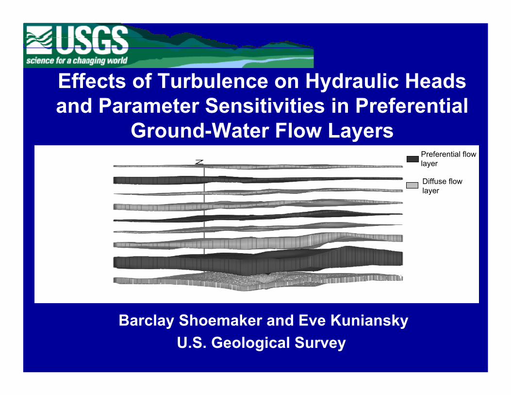
Effects of Turbulence on Hydraulic Heads and Parameter Sensitivities in Preferential
Ground-Water Flow Layers
Barclay Shoemaker and Eve Kuniansky U.S. Geological Survey
Preferential flow layer
Diffuse flow layer
Project Funded by USGS Ground-Water Resources ProgramKevin Dennehy, Program Manager
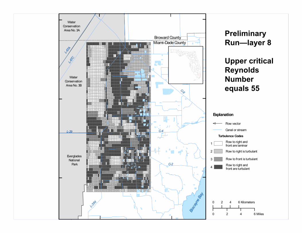
1. Extent of turbulent flow increases with increasing hydraulic conductivity, mean void diameter, groundwater temperature, and decreasing critical Reynolds numbers.
2. When turbulence was active (occurring in about 56% of preferential flow model cells), head differences from laminar elevations ranged from about 18 to +27 cm.
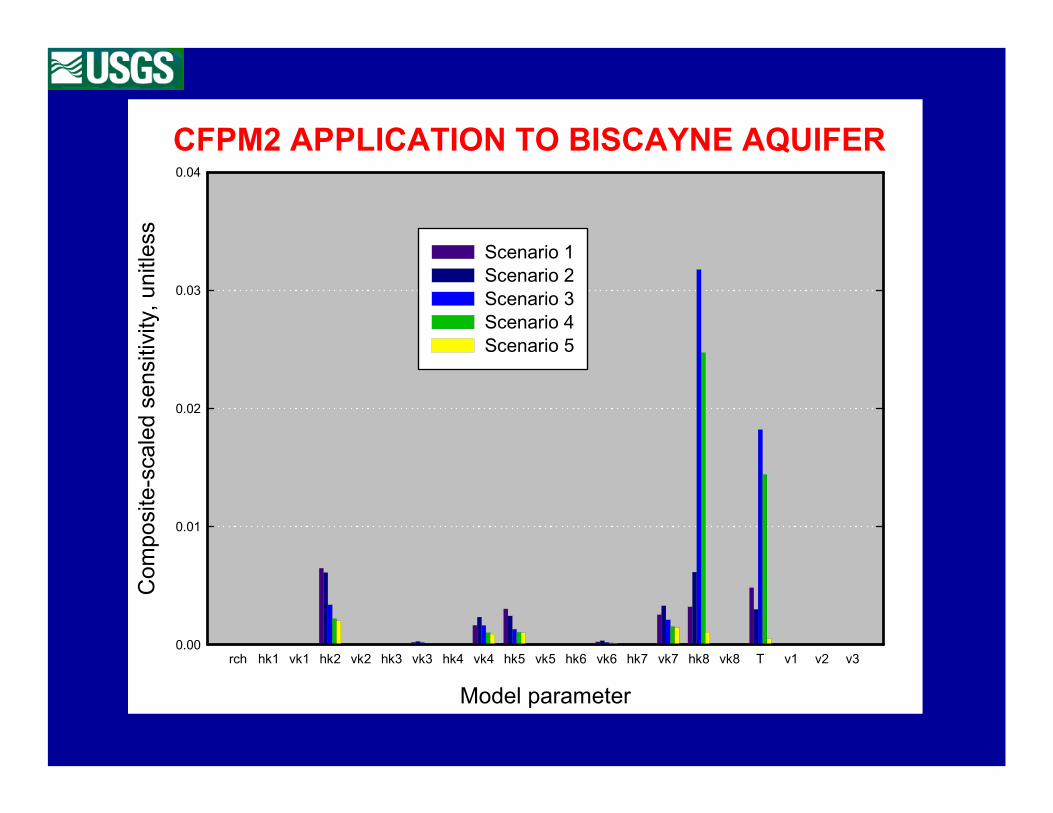
3. The composite-scaled sensitivities of horizontal hydraulic conductivities decreased by as much as 70% when turbulence was essentially removed.
4. This study highlights potential errors in model calculations based on the equivalent porous media assumption, which assumes laminar flow in uniformly distributed void spaces
Summary
Limitations
• Macro-scale simplification of impacts of turbulent flow
• Vast uncertainty in aquifer hydraulic properties and boundaries
• Theory is sound, but applications on systems with uncertainty may produce unreliable predictions
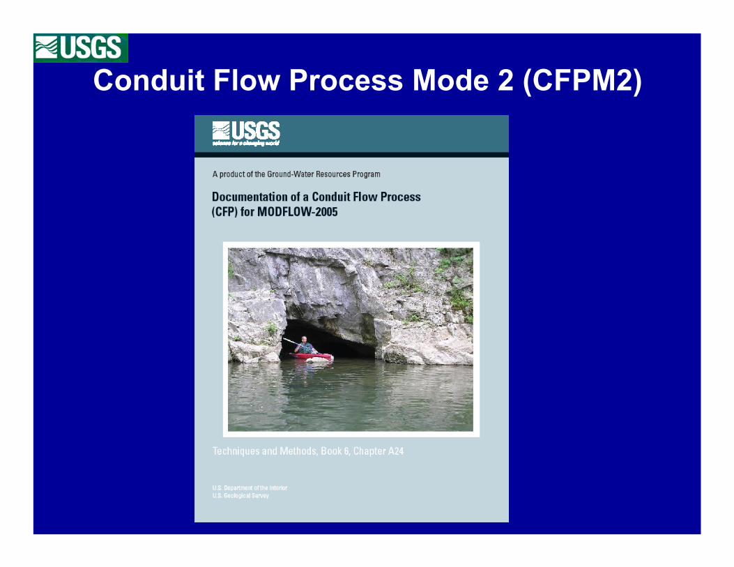
Picture taken by Eve Kuniansky of field trip to Fish River Cave near Yangshuo, China,
Shoemaker, W. B., K. J. Cunningham, E. L. Kuniansky, and J. Dixon (2008), Effects of turbulence on hydraulic heads and parameter sensitivities in preferential groundwater flow layers, Water Resour. Res., 44, W03501, doi:10.1029/2007WR006601.