Governors State UniversityOPUS Open Portal to University Scholarship

All Capstone Projects Student Capstone Projects

Fall 2010

Effects of Urbanization on EnvironmentalParameters in Aquatic Systems along an Urban-rural Gradient in Northeastern IllinoisTiffany GarrettGovernors State University

Follow this and additional works at: http://opus.govst.edu/capstones

Part of the Environmental Indicators and Impact Assessment Commons

For more information about the academic degree, extended learning, and certificate programs of Governors State University, go tohttp://www.govst.edu/Academics/Degree_Programs_and_Certifications/

Visit the Governors State Environmental Biology DepartmentThis Project Summary is brought to you for free and open access by the Student Capstone Projects at OPUS Open Portal to University Scholarship. Ithas been accepted for inclusion in All Capstone Projects by an authorized administrator of OPUS Open Portal to University Scholarship. For moreinformation, please contact opus@govst.edu.

Recommended CitationGarrett, Tiffany, "Effects of Urbanization on Environmental Parameters in Aquatic Systems along an Urban-rural Gradient inNortheastern Illinois" (2010). All Capstone Projects. 26.http://opus.govst.edu/capstones/26

CORE Metadata, citation and similar papers at core.ac.uk

Provided by Governors State University

Effects of Urbanization on environmental parameters in aquatic

systems along an urban-rural gradient in Northeastern Illinois

Garrett, Tiffany

Environmental Biology Program, Governors State University, IL

2

Abstract

The transformation of landscapes from rural to urban land use impacts affected

ecosystems. Replacing natural vegetation with impervious surfaces and introducing

environmental stressors through increased human activity can significantly alter aquatic

ecosystems. This study examined the effects that urbanization had on salinity, dissolved oxygen,

temperature, conductivity, and pH of aquatic systems along an urban-rural gradient in Illinois,

Chicago land area- Little Calumet River, Thorn Creek, and Kankakee River. The first objective

of this project was to examine whether there were changes or fluctuations among various

environmental parameters that may be due to heavily populated residential areas when compared

to a preserve. The second objective compared the responses of the environmental parameters

against the urban- rural gradient. The study was conducted from February to August 2010. Data

collection was from March to May 2010. There was a significant difference in all variables along

the urban-rural gradient based on location (p<0.001), date (p=0.001), and location date

interaction (p=0.001). Preserve sites had significantly higher salinity values than residential sites

(p=0.029). The values for examined parameters in the study ranged 3.45-17.10°C (temperature),

73.73-112.03 % saturation (dissolved oxygen), 352.33-1113.33 µS (conductivity), 0.20-0.50ppt

(salinity), and 7.80-8.90 (pH) in residential areas. While values ranged 3.60-17.23°C

(temperature), 42.67-104.23 % saturation (dissolved oxygen), 352.95-1299.57 µS (conductivity),

0.10-0.80ppt (salinity), and 7.20-8.87 (pH) in preserve areas respectively. On average, along the

urban-rural gradient there was a decrease in conductivity and salinity in residential areas.

Average values for parameters in the Little Calumet River residential site were 10.34±5.55 °C

(temperature), 8.18±0.28 (pH), 900.67±162.38 µS (conductivity), 0.49±0.03 ppt (salinity),

86.46±9.29 % saturation (dissolved oxygen). Average values for parameters in Thorn Creek

residential site ranged 8.93±4.10°C (temperature), 8.49±0.32 (pH), 522.11±154.60µS

3

(conductivity), 0.34±0.05ppt (salinity), 94.50±12.31 % saturation (dissolved oxygen). Average

values for parameters in the Kankakee River residential site ranged 11.23±3.49 °C (temperature),

8.27±0.32 (pH), 531.03±102.37 µS (conductivity), 0.29±0.04ppt (salinity), 86.99±7.36%

saturation (dissolved oxygen).On average, along the urban-rural gradient there was a increase in

dissolved oxygen, and a decrease in conductivity and salinity. Average values for parameters in

the Little Calumet River preserve sites ranged 11.36±3.64 °C (temperature), 8.08±0.51 (pH),

952.57±186.14 µS (conductivity), 0.59±0.13 (salinity), 71.70±21.21 % saturation (dissolved

oxygen). Average values for parameters in Thorn Creek preserve sites ranged 8.93±3.99°C

(temperature), 8.37±0.26 (pH), 612.68±212.83 µS (conductivity), 0.39±0.09ppt (salinity),

86.91±4.45 % saturation (dissolved oxygen). Average values for parameters in the Kankakee

River preserve site ranged 11.27±3.08 °C (temperature), 8.49±0.24 (pH), 473.90±96.10µS

(conductivity), 0.27±0.07ppt (salinity), 87.10±4.74% saturation (dissolved oxygen). The analysis

emphasize that aquatic systems are the product of their land, and the influence of aquatic systems

is driven by human pressures. The findings indicate that efforts should be stressed to preserve

and improve land in order to achieve a hydrological balance, thus creating a more habitable

aquatic ecosystem for aquatic plants and animals, and humans.

Keywords: Urban-Rural Gradient; Salinity; Dissolved Oxygen; Temperature; Conductivity;

Aquatic Ecosystem; population density; sustainable land use; pollution; environmental

parameters

4

1. Introduction

The disturbing impacts of urbanization on natural landscapes and habitats are expected to

continue to increase rapidly into the future (United Nations Human Settlements Programme,

2004). The process of urbanization can generate artificial and impervious surfaces (McDonnell

and Hahs, 2008). Urbanization, which is driven by human density, ultimately results in new land

cover types and biotic assemblages of plants and animals. In turn, this can alter the types and

frequency of disturbance regimes (McDonnell and Pickett, 1993; Kinzig and Grove, 2001).

Urbanization has the ability to alter the flux of nutrients, organisms, energy, and water within

and between landscapes (McDonnell and Hahs 2008).

Urbanization can cause habitat loss, changes in hydrology, increases in sedimentation and

pollution of water bodies, and changes in soil properties (Hamer and McDonnell 2008).

Replacing natural vegetation with impervious surfaces and introducing environmental stressors

through increased human activity can significantly alter aquatic ecosystems. Urban aquatic

systems suffer the most damage due to high population densities and pollution. Over 476,000 ha

of arable land are lost annually by the expansion of urban areas (Pouyat et al., 2002). Urban areas

such as Chicago have approximately 386 people/km², suburban locals such as Park Forest have

approximatley193 people/km² ,while rural areas such as Bourbonnais have population densities

less than 193 people/km²(United States Census Bureau 2010). In most cases urban land

conversion results in poor conditions for plant growth, with soil suffering from altered nutrient

5

fluxes or lacking essential nutrients (Pouyat et al., 2001). Previous studies have shown that soil

has a large capacity for retaining hydrophobic chemicals, which can alter soil nutrient levels

(Wong et al., 2004). Recent studies have found high conductivity (i.e., the presence of dissolved

metals and salts in water) to negatively affect animal species populations in urban areas (Hamer

and McDonnell 2008). Studies have shown that animal species like amphibians had lower

survival, growth, and development rates due to nitrogen pollution and heavy metals in urban

areas (Boone and Bridges, 2003; Casey et al., 2005; Massal et al., 2007). Blair (1996) reported a

decrease in species richness with urbanization in Coastal California, in addition to species being

methodically replaced along a more urbanized gradient.

Development of cities and small towns creates environmental conditions that can be

studied using gradient analysis (McDonnell and Hahs 2008). More than 50% of the world’s

population resides in urban areas (World Resources Institute, 1996). Studies have shown waste

incineration, vehicle exhaust, and cigarette smoke to be the main sources of urban pollution.

Urban areas are in close proximity with these sources; and urban residents have higher health

risks. Knowledge of our residential environmental parameters should be a major concern because

where one lives affects his or her educational opportunity, quality of life, and access to health

care (Billard 1993). Research on urbanization allows scientists the opportunity to survey how

natural communities are structured and function under dramatically altered landscapes (Blair and

Johnson 2008). Also, environmentally sustainable land use and conservation are necessary to

avoid species extinction (Blair and Johnson 2008). It is apparent that urbanization disrupts our

6

natural ecosystems in addition to posing a major threat to biota. More ecological information

would help increase the number of inhabitable cities and help achieve better research,

management, restoration, and conservation outcomes (McDonnell and Hahs 2008).

Two related variables are water temperature and dissolved oxygen. Water temperature

and dissolved oxygen are inversely related environmental variables crucial to the survival of

aquatic organisms and their ability to resist certain pollutants. Large industrial businesses such as

power plants use water for cooling purposes and released water can affect downstream habitats.

Low levels of dissolved oxygen indicate eutrophication in which water quality is reduced and

organisms begin to die. Also associated with eutrophication is high turbidity, during which

sunlight cannot pass through dense and gray colored water, causing excess organic material and

low levels of oxygen. Phosphorous is a pollutant that causes eutrophication of aquatic systems

(Bennett 2003). Soil phosphorous moves downhill into aquatic systems from sorbed to eroded

soil particles and are dissolved in surface runoff and groundwater (Bennett 2003).

Also related to dissolved oxygen are water pH, conductivity and salinity. The pH of the

water can be affected by chemicals in the water. It is important that the pH remains stable and

within certain limits for organisms to survive and thrive. Jennifer et. al (2006) reported that

changes in pH values resulted in changes in species abundance and interactions with other

organisms. The amount of dissolved solids in the water impacts its ability to conduct an electrical

current. High specific conductance can affect the suitability of water for domestic, industrial, and

7

agricultural use. High levels of conductance may affect the taste and odor of drinking water and

may cause gastrointestinal distress. Likewise, high salinity may inhibit survival of nearby crops.

Impervious surfaces may contribute to nutrient loss, high salinity, high conductivity, and changes

in pH and dissolved oxygen (Environmental Protection Agency 2007).

Similarly, another study reported that anthropogenic changes in water salinity,

conductivity, dissolved oxygen, and temperature affected species survival and interspecific

interactions (U.S. Geological Survey 2005) .Comparison of aquatic systems in urban areas with

surrounding rural areas should help identify trends in environmental variables associated with

decline in water quality. In addition, regional aquatic systems can provide a baseline against

which potentially more intense human activity in urban areas can be judged (Cannon and Horton

2009).

Previous studies that examined larger areas are too broad to capture the specific historical

patterns which have developed within these areas. Many studies provide information of how

animals are affected, but have no underlying contextual dynamics that explain how their

observations came to be. The precise magnitude of urbanization can only be measured by the

environments response, which is why air, soil, and water quality testing are vital. There is an

increasing awareness of problems caused by environmental degradation, due to increasing

demands placed on the environment by population growth. A study of some key physical and

chemical characteristics from the Little Calumet River, Thorn Creek, and the Kankakee River

will help expand local knowledge of these aquatic systems, and is also essential for effective

8

management and restoration policies and procedures. This research addresses water quality traits

related to surrounding land cover of natural and developed aquatic ecosystems. In addition, the

study examines how environmental parameters vary across different land-use types along the

urban-rural gradient.

The overall object of this research investigated the effects that urbanization had on

environmental variables including salinity, dissolved oxygen, temperature, conductivity, and pH,

along an urban-rural gradient from Chicago to rural Kankakee (Fig. 1). Changes in

environmental parameters may impact plant and animal life. This research provides information

of a gradient that can be used to establish basic ecological research in areas where previous

information is absent. This research also provides a common element that allows for a greater

integration between studies conducted at different places. In this study, the southern part of

Chicago is designated as the high density urban area, Park Forest is south of Chicago and is the

less heavily populated suburban area, and Bourbonnais located south of Park Forest is the least

heavily populated and is designated the rural area.

Fig 1. of Urban-Rural Gradient Map

9

This study examined how urbanization affects water quality. I hypothesized that

urbanization would have an effect on the parameters and that changes will be noted along the

urban rural gradient. It is expected that each city will have its own characteristic aquatic

signature determined by the history of land use. It was expected that the urban end of the

gradient, Little Calumet River and residential plots will fail to meet EPA criteria for water

quality standards. The changes are indicative of harmful increases in salinity, and decreases in

dissolved oxygen which may disrupt aquatic plant and animal processes. Higher levels of salinity

and conductivity and lower levels of dissolved oxygen were found at the Little Calumet River

and did not meet EPA criteria. The Little Calumet River is located within the urban area of

Chicago. Water bodies near heavily populated areas may be less suitable for species survival

than water bodies near preserves. The Chicago city area provides an excellent opportunity for

studying the effects of urban-rural land-use gradient on water quality due to its vast economic

and industrial history.

2. Materials and Method

2.1. Study Area

The study was conducted in the Chicago City and surrounding suburban and rural area.

The urban-rural gradient included water bodies near three cities in Illinois. All plots can be

accessed from Interstate 57 which runs North and South. The city of Chicago and its surrounding

suburban and rural areas have an industrial, environmental and demographic history. Chicago is

located in Cook County, Illinois and houses approximately 9.7 million human residents (United

10

States Census Bureau 2010), and is the third largest city in the United States. Park Forest is a

village located south of Chicago, in Cook County, Illinois. It has a population of 23,462 human

residents (United States Census Bureau 2010). Bourbonnais is a village in Kankakee County,

Illinois and has a population of 15, 256 human residents (United States Census Bureau 2010). As

of April 2010, there is a lack of adequate bedrock geologic knowledge for Kankakee County,

Illinois (Leib, Susan E. 2010).

Ecosystems in Illinois include forests, farmland, prairies, wetlands, lakes, urban areas,

and rivers. Illinois has a temperate climate with cold snowy winters, and hot wet summers.

Average winter temperatures are approximately -5.5°C in the north and 2.7 °C in the south.

Mean summer temperatures are 21.1°C in the north and 25 °C in the south. Average rainfall is

approximately 91.44 cm per year, and annual snowfall is 93.98 cm for northern Illinois and

154.84 cm central and southern Illinois. During the study period average temperatures of the

coldest month (March) to the warmest (May) were approximately 6.6°C to 18.8°C respectively.

Little Calumet River

The Little Calumet River study area is at the urban end of the urban-rural gradient and

has 175.4 km of river and tributaries. The Little Calumet River originates at the east end of Gary,

IN and flows through South Chicago, IL and Gary IN. The majority of the river flow drains in

Lake Michigan. The Little Calumet River flows through or borders the towns of Blue Island,

11

Burnham, Dixmoor, Phoenix, Riverdale, Harvey, Calumet City, Lansing, Dolton, and South

Holland in Illinois; and Hammond, Munster, Griffith, Highland, Gary, Lake Station, Portage,

Burns Harbor, Porter, and Chesterton in Indiana. The city of Chicago, IL with its dense

population is located within the northeastern part of Illinois and lies along the southwestern tip of

Lake Michigan. The city lies between two rivers, -the Chicago and the Calumet Rivers. The city

occupies an area of 606.2km² and according to the US Census Bureau has a combined residential

and industrial of approximately 9.7 million people. South Chicago from 130th

to 138th

street east

of the Bishop Ford freeway and west of the Little Calumet River is home to almost 1,000

residents. It is .77km² and located northwest of a disposal site, numerous manufacturing plants,

former steel mills, waste dumps, and landfills. The Calumet River in the Chicago area is

surrounded by houses, factories, and a waste management facility. It is not easily accessible to

the surrounding community or visitors as a recreational park facility. Study site 1 (preserve)

(Lon 87.83682 W, Lat 41. 14431 N) is located east of Interstate 57 and is the Little Calumet boat

docking area. The area is surrounded by woodlands and is also directly across from houses and a

nearby machinery facility. Study site 2 (residential) ( Lon 87.56061 W, Lat 41.64822 N) is

located at a Chicago Marina. This site is surrounded by houses, nearby roads, and the river flows

directly around a waste management facility.

Thorn Creek

The Thorn Creek study area is located in Park Forest, Illinois approximately 40.2 km

south of the city of Chicago and represents the middle location along the urban-rural gradient.

12

Thorn Creek is a sub-watershed of the larger Chicago watershed. Its tributaries include

Butterfield Creek, Deer Creek, and North Creek. 105 km of stream wind through 26936 ha of

northeastern Illinois and 777 ha of northwestern Indiana. Most streams of the Thorn Creek

watershed flow from southwest to northeast from their origins in Eastern Will County to their

confluence with Thorn Creek and continue to the Little Calumet River in southern Cook County.

Park Forest can be accessed from Interstate 57. It is surrounded by U.S. Highway 30 to the north,

Western Avenue on the east, the Canadian National Railway to the west and Thorn Creek to the

south. Thorn Creek is approximately 336 hectares and runs from a preserve where the nature

center is located through a residential neighborhood along Monee Road. Thorn Creek Preserve

became an Illinois State Nature Preserve in 1978, and consists of floodplain to mesic deciduous

forest, wetlands, and tall grass prairie communities. Study site 1 (preserve) of Thorn Creek is

located approximately 1.12 km east from the start of the trail near the nature center ( Lon

87.69867 W, Lat 41.46032 N). Study site 2 (residential) is located approximately .06 km east of

W Steger Road (Lon 87.67148 W, Lat 41.46979 N). Houses are located within .02 km to the east

and south of the study site.

Kankakee River

The Kankakee River study area is at the rural end of the gradient. It is located in

Bourbonnais, Illinois and is approximately 88.5 km south of the city of Chicago. The Kankakee

River, a tributary of the Illinois River is approximately 144.8 km long in northwestern Indiana

and northeastern Illinois. The river rises in northwest Indiana, approximately 8.05 km southwest

13

of South Bend. The river curves westward as it enters Kankakee County in northeastern Illinois.

Approximately 4.8 km southeast of the city of Kankakee, the Kankakee River receives the

Iroquois River from the south and turns sharply to the northwest for its lower 56.3 km. It joins

the Des Plaines River from the south to form the Illinois River, approximately 80.5 km

southwest of Chicago. The river can be accessed from Interstate 57 or 55 and Illinois Routes 102

on the north and 113 on the south. Study site 1 (preserve) of the Kankakee River is located at

Kankakee River State Park (Lon 87.69867 W, Lat 41.46032 N) with floodplain forest cover.

Study site 2 (residential) is located off of US-45, N Kennedy Drive (Lon 87.87680 W, Lat

41.12272 N) with roads 0.5 km to the north, east, and south of the site. Land uses adjacent to the

site include a baseball field west of the site, and a construction site (Johnson Downs Construction

Inc.). In addition, local communities and hospitals are located within 3.2 km northwest of the

site. The Kankakee River is a woodland area and has a vast animal population of fox, coyote,

deer, badgers, beavers, turtles, wild turkeys, red-winged black birds, herons, bluebirds, frogs,

snakes, dove, woodcock, rabbit, squirrel, raccoon, and many others.

2.2. Experimental design

In this study, an urban-rural gradient based on population density in southern Chicago

and the surrounding suburban and rural areas was selected. The urban-rural gradient contained 3

cities in Illinois- Chicago, Park Forest, and Bourbonnais with population densities >386

people/km², 193 people/km², and <193 people/km² for the three cities, respectively. In each

study site, two plots which represented residential and preserve areas were chosen. Data was

14

collected at Little Calumet River (Chicago), Thorn Creek (Park Forest) and Kankakee River

(Bourbonnais). Handheld meters were randomly placed and fully submerged in the water at three

random locations for each body of water plot biweekly from March to May 2010.

2.3. Water sampling

Samples were collected three times in March 2010 and two times in April 2010 and May

2010 between 8:00am to 1:00 pm CDT. At each of the three locations- Kankakee River, Thorn

Creek, and Little Calumet River, samples were collected at preserve and residential sites. For

each sample a YSI Model 85 handheld portable meter (YSI Inc, Yellow Springs, OH, USA) was

used to measure dissolved oxygen, conductivity, salinity, and temperature of water. A Hanna HI

9812-5 portable multi-meter (Hanna Instruments, Inc., Woonsocket, RI, USA) was used to

measure water pH. During each sample collection date at each sampling site, measurements of

environmental variables were made at three random locations and averaged. The probe end of

each meter was dipped into the sub surface area (approximately 0.001 km) of the water while the

digital value was read and recorded. Dissolved oxygen was measured in percent saturation (%

sat.), conductivity in micro Siemens per centimeter (µS/cm), salinity in parts per thousand (ppt),

and temperature in degrees Centigrade (°C).

2.4. Statistical Analysis

Two analyses were conducted to determine if the environmental parameters were affected

by heavily populated residential areas and if water bodies near the urban end of the gradient

15

differed significantly from the rural end of the gradient. A two-tailed t-test using mean values

was performed to test the null hypothesis that there are no differences in dependent variables-

dissolved oxygen, temperature, pH, salinity, and conductivity when comparing preserve vs.

residential aquatic systems at three locations along an urban-rural gradient. A repeated measures

MANOVA analysis conducted on differences between preserve and residential mean values was

used to test three null hypotheses that there are no overall differences in environmental variables

of aquatic systems at three locations along an urban-rural gradient based on location, date, and

(date x location) interaction.

3. Results

Preserve sites had significantly higher salinity values than residential sites (p=0.029) (Fig

2.). There were no significant differences in residential and preserve sites for environmental

parameters water pH, dissolved oxygen, temperature, and conductivity. The results showed that

average values for parameters in residential areas for temperature ranged 3.45-17.1°C, dissolved

oxygen 73.73-112.03 % saturation, conductivity 352.33-1113.33 µS, salinity 0.2-0.5 ppt, and pH

7.8-8.9. Average values for parameters in preserve areas for temperature ranged 3.6-17.23°C,

dissolved oxygen 42.67-104.23 % saturation, conductivity 352.95-1299.57 µS, salinity 0.1-0.8

ppt, and pH 7.2-8.87 (Table 1.)

16

There was a significant difference in all variables along the urban-rural gradient based on

location (p<0.001), date (p=0.001), and location date interaction (p=0.001) (Table 2). The values

for examined parameters in the study ranged 3.45-17.10°C (temperature), 73.73-112.03 %

saturation (dissolved oxygen), 352.33-1113.33 µS (conductivity), 0.20-0.50ppt (salinity), and

7.80-8.90 (pH) in residential areas. While values ranged 3.60-17.23°C (temperature), 42.67-

104.23 % saturation (dissolved oxygen), 352.95-1299.57 µS (conductivity), 0.10-0.80ppt

(salinity), and 7.20-8.87 (pH) in preserve areas respectively. On average, along the urban-rural

gradient there was a decrease in conductivity and salinity in residential areas. Average values for

parameters in the Little Calumet River residential site were 10.34±5.55 °C (temperature),

8.18±0.28 (pH), 900.67±162.38 µS (conductivity), 0.49±0.03 ppt (salinity), 86.46±9.29 %

saturation (dissolved oxygen)(Table 3). Average values for parameters in Thorn Creek

residential site ranged 8.93±4.10°C (temperature), 8.49±0.32 (pH), 522.11±154.60µS

(conductivity), 0.34±0.05ppt (salinity), 94.50±12.31 % saturation (dissolved oxygen)(Table 4).

Average values for parameters in the Kankakee River residential site ranged 11.23±3.49 °C

(temperature), 8.27±0.32 (pH), 531.03±102.37 µS (conductivity), 0.29±0.04ppt (salinity),

86.99±7.36% saturation (dissolved oxygen)(Table 5).On average, along the urban-rural gradient

there was a increase in dissolved oxygen, and a decrease in conductivity and salinity. Average

values for parameters in the Little Calumet River preserve sites ranged 11.36±3.64 °C

(temperature), 8.08±0.51 (pH), 952.57±186.14 µS (conductivity), 0.59±0.13 (salinity),

71.70±21.21 % saturation (dissolved oxygen)(Table 3). Average values for parameters in Thorn

Creek preserve sites ranged 8.93±3.99°C (temperature), 8.37±0.26 (pH), 612.68±212.83 µS

(conductivity), 0.39±0.09ppt (salinity), 86.91±4.45 % saturation (dissolved oxygen)(Table 4).

Average values for parameters in the Kankakee River preserve site ranged 11.27±3.08 °C

17

(temperature), 8.49±0.24 (pH), 473.90±96.10µS (conductivity), 0.27±0.07ppt (salinity),

87.10±4.74% saturation (dissolved oxygen)(Table 5). The range of environmental parameters for

residential and preserve sites in the Little Calumet River, Thorn Creek, and Kankakee River are

shown in Tables 6 and 7.

Environmental variables in all three locations were significantly different due to location

and date. Residential mean values were subtracted from preserve values to compare differences

in preserve and residential sites. This eliminates the residential and preserves plots, thus allowing

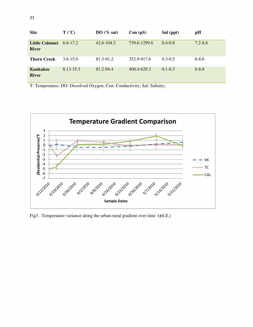
for comparison of only the urban-rural gradient. Temperature values at the Little Calumet River

were higher for preserve sites in early spring and higher for residential sites in late spring. Thorn

Creek Values were higher for preserve sites in early spring. (Fig 3.) Dissolved Oxygen values at

the Little Calumet River were higher for preserve sites in early and mid spring. Values for

residential sites were higher in late spring. Thorn Creek Values were higher at residential sites

for early and mid spring. Kankakee values were higher for residential sites in mid spring. (Fig 4.)

Conductivity values at the Little Calumet River were higher in preserve sites in early spring and

mid spring; residential values were higher in late spring. Values at Thorn Creek were higher at

preserve sites in mid spring; values at the Kankakee River were higher for residential sites in mid

spring. (Fig 5.) Salinity values at the Little Calumet River site were higher for preserve sites in

early and mid spring. Thorn Creek values were higher for preserve sites in early spring.

Kankakee values were higher for residential sites in mid spring. (Fig 6.) pH values for the Little

calumet River were higher for preserve sites in early spring and higher for residential sites in late

spring. Thorn Creek values were higher for residential in early, mid, and late spring. Kankakee

values were higher for preserve sites in early and mid spring (Fig 7.).

18

Fig 2. Average salinity values for preserve and residential sites

Table 1.Range of environmental parameters values for residential and preserve plots*

Plots T (°C) DO (% sat) Con (µS) Sal (ppt) pH

Residential 3.45-17.1 73.73-112.03 352.33-

1113.33

0.2-0.5 7.8-8.9

Preserve 3.6-17.23 42.67 352.95-

1299.67

0.1-0.8 7.2-8.887

T: Temperature; DO: Dissolved Oxygen; Con: Conductivity; Sal: Salinity;

Table 2. P values-MANOVA analysis

0

0.1

0.2

0.3

0.4

0.5

0.6

3-Mar 13-Mar 23-Mar 2-Apr 12-Apr 22-Apr 2-May 12-May 22-May 1-Jun

Sa

l (p

pt)

Dates 2010

Salinity Trend

res

pre

p-value=0.029

19

Source Wilk’s Lambda (Pr>F)

Location (Within

Subjects)

0.001

Date (Between

Subjects)

<0.001

Location-Date

(Between Subjects)

<0.001

Table 3.Mean environmental parameter values for residential and preserve plots of The Little Calumet

River*

Little

Calumet

River

Plots T (°C) DO (% sat) Con (µS) Sal (ppt) pH

Residential 10.34±5.55 86.46±9.29 900.67±162.38 0.49±0.03 8.18±0.28

Preserve 11.36±3.64 71.90±21.21 952.57±186.14 0.59±0.13 8.08±0.51

T: Temperature; DO: Dissolved Oxygen; Con: Conductivity; Sal: Salinity;

Table 4.Mean environmental parameter values for residential and preserve plots for Thorn Creek*

Thorn Creek

Plots T (°C) DO (% sat) Con (µS) Sal (ppt) pH

Residential 8.93±4.10 94.50±12.31 522.11±154.60 0.34±0.05 8.49±0.32

Preserve 8.93±3.99 86.91±4.45 612.68±212.83 0.39±0.09 8.37±0.26

T: Temperature; DO: Dissolved Oxygen; Con: Conductivity; Sal: Salinity;

20

Table 5. Mean environmental parameter values for residential and preserve plots for The Kankakee

River*

Kankakee

River

Plots T (°C) DO (% sat) Con (µS) Sal (ppt) pH

Residential 11.23±3.49 86.99±7.36 531.03±102.37 0.29±0.04 8.27±0.32

Preserve 11.27±3.08 87.10±4.74 473.90±96.10 0.27±0.07 8.49±0.24

T: Temperature; DO: Dissolved Oxygen; Con: Conductivity; Sal: Salinity;

Table 6.Range of environmental parameter values for Residential sites across the urban-rural gradient*

Site T (°C) DO (% sat) Con (µS) Sal (ppt) pH

Little Calumet

River

3.45-17.1 74.13-96.6 671-1113.3 0.4-0.5 7.8-8.7

Thorn Creek 4.26-15.16 81.23-112.03 352.3-733.3 0.3-0.4 8.13-8.9

Kankakee

River

7.65-15.86 73.3-93.3 446.4-669.6 0.2-0.3 7.95-8.41

T: Temperature; DO: Dissolved Oxygen; Con: Conductivity; Sal: Salinity;

Table 7. Range of environmental parameter values for Preserve sites across the urban-rural gradient*

21

Site T (°C) DO (% sat) Con (µS) Sal (ppt) pH

Little Calumet

River

6.6-17.2 42.6-104.2 739.6-1299.6 0.4-0.8 7.2-8.6

Thorn Creek 3.6-15.0 81.3-91.2 352.9-917.6 0.3-0.5 8-8.6

Kankakee

River

8.13-15.3 81.2-94.4 400.4-629.3 0.1-0.3 8-8.8

T: Temperature; DO: Dissolved Oxygen; Con: Conductivity; Sal: Salinity;

Fig3 . Temperature variance along the urban-rural gradient over time (±S.E.)

-7

-6

-5

-4

-3

-2

-1

0

1

2

3

(Re

sid

en

tia

l-P

rese

rve

)°F

Sample Dates

Temperature Gradient Comparison

KK

TC

CAL

22

Fig 4.Dissolved Oxygen variance along the urban

Fig 5. Conductivity variance along the

-20

-10

0

10

20

30

40

(Re

sid

en

tia

l-P

rese

rve

) %

Sa

t.Dissolved Oxygen Gradient Comparison

-800

-600

-400

-200

0

200

400

(Re

sid

en

tia

l -

Pre

serv

e)

µS

Conductivity Gradient Comparison

early spring mid spring late spring

4.Dissolved Oxygen variance along the urban-rural gradient over time (±S.E.)

Fig 5. Conductivity variance along the urban-rural gradient over time (±S.E.)

Sample Dates

Dissolved Oxygen Gradient Comparison

Sample Dates

Conductivity Gradient Comparison

spring mid spring late spring

KK

TC

CAL

KK

TC

CAL

23

Fig 6. Salinity variance along the urban-rural gradient over time (±S.E.)

Fig 7. pH variance along the urban-rural gradient over time (±S.E.)

-0.35

-0.3

-0.25

-0.2

-0.15

-0.1

-0.05

0

0.05

0.1

0.15

(Re

sid

en

tia

l-P

rese

rve

) p

pt

Sample Dates

Salinity Gradient Comparison

KK

TC

CAL

-1

-0.8

-0.6

-0.4

-0.2

0

0.2

0.4

0.6

0.8

1

(Re

sid

en

tia

l-P

rese

rve

)

Sample Dates

pH Gradient Comparison

KK

TC

CAL

24

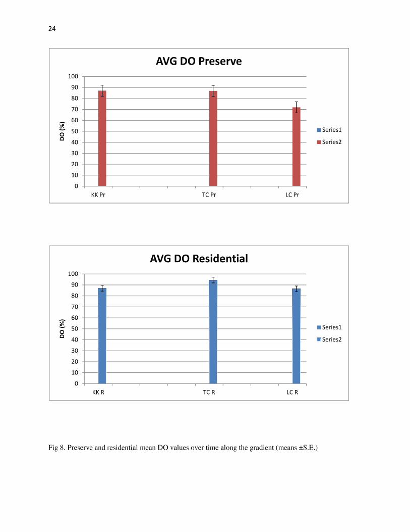
Fig 8. Preserve and residential mean DO values over time along the gradient (means ±S.E.)

0

10

20

30

40

50

60

70

80

90

100

KK Pr TC Pr LC Pr

DO

(%

)AVG DO Preserve

Series1

Series2

0

10

20

30

40

50

60

70

80

90

100

KK R TC R LC R

DO

(%

)

AVG DO Residential

Series1

Series2

25

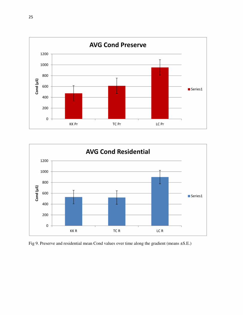
Fig 9. Preserve and residential mean Cond values over time along the gradient (means ±S.E.)

0

200

400

600

800

1000

1200

KK Pr TC Pr LC Pr

Co

nd

(µ

S)

AVG Cond Preserve

Series1

0

200

400

600

800

1000

1200

KK R TC R LC R

Co

nd

(µ

S)

AVG Cond Residential

Series1

26

Fig 10. Preserve and residential mean Sal values over time along the gradient (means ±S.E.)

0.00

0.10

0.20

0.30

0.40

0.50

0.60

0.70

0.80

KK Pr TC Pr LC Pr

Sa

lin

ity

(p

pt)

AVG Sal Preserve

Series1

0.00

0.10

0.20

0.30

0.40

0.50

0.60

0.70

0.80

KK R TC R LC R

Sa

lin

ity

(p

pt)

AVG Sal Residential

Series1

27

Fig11. Preserve and residential Temp values over time along the gradient

0.00

2.00

4.00

6.00

8.00

10.00

12.00

14.00

16.00

18.00

20.00

3/3 3/13 3/23 4/2 4/12 4/22 5/2 5/12 5/22 6/1

Te

mp

era

ture

(°C

)

Dates 2010

Temperature (Pres)

Cal pre

TC pre

KK Pre

0.00

2.00

4.00

6.00

8.00

10.00

12.00

14.00

16.00

18.00

3/3 3/13 3/23 4/2 4/12 4/22 5/2 5/12 5/22 6/1

Te

mp

era

ture

(°C

)

Dates 2010

Temperature (Res)

Cal res

TC res

KK res

28

Fig 12. Preserve and residential pH values over time along the gradient

4.00

5.00

6.00

7.00

8.00

9.00

10.00

3/3 3/13 3/23 4/2 4/12 4/22 5/2 5/12 5/22 6/1

pH

Dates 2010

pH (Pres)

Cal pre

TC pre

KK Pre

7.60

7.80

8.00

8.20

8.40

8.60

8.80

9.00

3-Mar 13-Mar 23-Mar 2-Apr 12-Apr 22-Apr 2-May 12-May 22-May 1-Jun

pH

Dates 2010

pH (Res)

Cal res

TC res

KK res

29

Table. 8 Comparison of results to EPA water quality standards*

T(°C) DO (% sat) Con (µS) Sal (ppt) pH

Lowest 3.5(Cal)

March

41.5 (Cal)

May

336.4 (Cal)

April

.1 (KK)

April

7.9 (KK)

March, May

Highest 17.3 (TC)

May

112.7 (TC)

March

1301(Cal)

April

.8 (Cal)

March

9.0 (TC)

March

Res (avg) 10.38±4.26 89.07±10.17 653.80±218.37 0.37±0.09 8.32±0.31

Pre (avg) 10.64±3.62 81.78±14.31 686.08±259.60 0.41±0.16 8.30±0.40

EPA Criteria

0-32 °C 80-120% 0-800µS/cm 0-.5ppt 5-9

T: Temperature; DO: Dissolved Oxygen; Con: Conductivity; Sal: Salinity; Res (avg): Residential

averages; Pre (avg): Preserve averages; Cal: Little Calumet River; TC: Thorn Creek; KK: Kankakee River

4.Discussion

In all natural ecosystems such as streams and rivers changes are likely to occur through

time. Over a geologic scale major changes occur, over a small scale such as a human lifespan

changes are so gradual that they are nearly undetectable. When an ecosystem is disturbed due to

human activity, these changes are accelerated. One of the most common changes is alterations in

the volume of water flowing through a river or stream channel. In this study preserve sites had

higher salinity volumes than residential ones. This may be due to construction of impervious

surfaces such as nearby parking lots, which alter the direction of stream flow. Residential sights

may have also had a downstream flow which ultimately results in an increase in water volume.

Although there were no significant differences in residential and preserve sites for the

environmental parameters except for salinity, measurements across the urban-rural gradient

30

indicate strong variations associated with the Little Calumet River’s dissolved oxygen,

conductivity, salinity (Fig8-10).

The Calumet River showed the most instability, values varied significantly from the

Kankakee River and Thorn Creek over a period of time. There was a major decrease in dissolved

oxygen at the preserve site in May (Fig 8). And during the study period the Little Calumet River

had the highest conductivity and salinity values when compared to Thorn Creek and the

Kankakee River (Fig 9-10). It is suggested that urbanization has had an effect on this particular

aquatic system which have shown to have increased levels of dissolved solids and the lowest

photosynthetic activity from plants and animals. The Kankakee River had slight variations but

overall proved to be more stable than the other two sites. The Kankakee River had a balance

within all parameters and over time didn’t have any extreme measurements. Environmental

parameters for this aquatic system proved to be less affected by human activity. The rural aquatic

system doesn’t suffer from the dangers of urbanization. Thorn Creek had the highest dissolved

oxygen, temperature, and pH measurements (Fig 8., 11.-12.), this may be due to the lack of cover

in the canopy surrounding the creek. Sunlight and rain was better able to reach the surface of the

water, therefore photosynthetic activity from aquatic plants and animals were heightened causing

an increase in dissolved oxygen levels. This particular suburban site had nearby roads and lacked

local manufacturing companies. This may account for the high pH levels in the creek due to the

lack of atmospheric pollution and the amount of unpolluted precipitation. Kankakee River had

the lowest salinity and pH measurements.

31

Aerial photographs of the three locations (Fig 13.) illustrate changes in land cover along

the gradient. The amount of land cover is directly proportional to the amount of urbanization,

thus more variation and extreme measurements were found in the Calumet River (lowest

temperature, lowest dissolved oxygen, lowest and highest conductivity, and highest salinity-

(Table 8.) when compared to the other two locations. The density of roads might be useful for a

study of the dispersal of mammals in an urban area, but a map of land cover is more useful for a

study of changes in water bodies along a gradient (Hahs and McDonnell 2006).

Fig 13. Aerial Maps of cities-1. Bourbonnais 2. Park Forest 3. Chicago

Fig.10.. Aerial Maps of Cities -

1 Bourbonnais, 2. P ark Fo rest, 3. Chicago

1.

2. 3.

Kankakee

River

Thorn Creek

Little Calumet River

Rural

(U rban Rural Gradient)

Urban

� ---------- --------------------------------------------------------------------------------------------------------- �

32

Many studies on eutrophication (Beeton 1965), sulphur contamination of rivers (Berner

1971), and general degradation of river quality (Wolman 1971), have been conducted on

urbanization and how human pressures are leading to global change in aquatic systems. The

results from this analysis over a three month period within less than a 96km gradient revealed a

great amount of variance within the aquatic systems, which prove that the security of future

water resources is threatened and that urbanization does in fact play a role. The hydrological

balance is dependent on transfer of river material, such as carbon and nutrient balance, and

biodiversity (Meybeck 2003), so one ecosystem can create global effects. Due to the amount of

variation at the Little Calumet River, it can be concluded that the water resources are not

exploited in an optimal way. Surface water transfers from the Little Calumet River are modified

through extensive land cover (urbanization) and past and present industrialization from nearby

factories, power plants, and waste facilities (Fig 14). According to Meybeck 2003, one of the

most common uses of water is still dilution and downstream transfer of waste. Deep saline

ground water is pumped and connected to surface water increasing river fluxes of nutrients and

pollutants. Salinization, which was found to have a significant difference in preserve sites and in

the Little Calumet River for this study, results from increase of sodium, chloride, and sulfate due

to industrial and mining wastewaters or from poor irrigation practices (Chilton 1989). This can

cause water use limitations and is indicative of early warning degradation of water quality.

33

Fig. 14 Maps of Environmental waste locations

Salinity has been viewed as one of the most important variables influencing the

utilization of organisms in aquatic systems. The Little Calumet River had the most and only

extreme values which fell either below or above EPA criteria (Table 8). Due to high salinity and

conductivity readings at the Little calumet River, dissolved oxygen concentrations were low.

With increased salinity and conductivity, dissolved oxygen in water decreases. The presence of

salts limits the amount of oxygen that can dissolve in water, and can be indicative of water

pollution and contamination. Freshwater holds more oxygen than salt water, so the oxygen

content can affect the reaction rates of aquatic plants and animals. Dissolved oxygen depletion

could suppress respiration, cause death of fish, depress feeding behavior, and affect embryonic

development. Water temperature correlated significantly with pH, but has no significant

correlation with salinity, conductivity, and dissolved oxygen. From March to May as water

temperature increased there was a decrease in pH. This may be due to the rainy months and the

Chicago

Park Forest

Kankakee

(Bourbonnais)

34

amount of acid rain from sulfur and nitrogen atmospheric pollution. The results from the

statistical analysis showed significant correlations between the variables at the three different

aquatic systems.

5. Conclusion

The analysis emphasize that aquatic systems are the product of their land, and the influence

of aquatic systems is driven by human pressures. If an ecosystem cannot sustain plant and lower

animal species life, eventually human life will become unsustainable. Urban areas provide a

gateway for invasive species, which result in increased erosion, elimination of vegetation, and

removal of food sources for many native species. It is no doubt that aquatic systems of this era

are no longer controlled by only Earth system processes. Aquatic system variation is directly

influenced by flood regulation, fragmentation, sediment balance, neo-arheism, salinization,

chemical contamination, acidification, eutrophication, and microbial contamination. As a result,

measures of urbanization capture the greatest variability within aquatic systems and are

indicative of water quality output.

The findings indicate that efforts should be stressed to preserve and improve land in order to

achieve a hydrological balance. Even though there are organizations such as the Environmental

Protection Agency (EPA) and Illinois Conservation Reserve Program (ICR) urban aquatic

35

systems still suffer from contamination and pollution. Legal history investigations have found

that penalties for failure to meet environmental regulations are lower in urban areas. Although

discharges have been reduced, contaminates continue to impair the area. And delays of site

approval in low income areas are longer as well. This research has revealed an imbalance at the

Little Calumet River test site. Further research should be proposed to determine how to reduce

pollution in and around the River, and enforce water regulation laws. Future research should

demonstrate ways to correct the water quality balance in order to make it available for

recreational activities and aquatic survival.

There should be a greater focus on preventive management and remediation engineering

solutions. These goals should include waste minimization, resource recovery, pollution

prevention, and consideration of environmental effects during product development. Future

environmental health programs should be strongly considered and emphasize efficient

monitoring of environmental quality, interpretation of the impact of human actions on terrestrial

and aquatic ecosystems, and a urgent need to comply with environmental laws and regulations

regarding ground water decontamination and clean air.

Acknowledgements

I would like to thank my committee advisors- Dr. Xiaoyong Chen, Dr. Mary Carrington,

and Dr. Phyllis Klingensmith for their support, patience, and good judgment. I would like to

thank Dr. Jon Mendelson for his review, helpful comments and suggestions, Ms.Sharon Browne

for help with documentation, Dr. Karen D’Arcy for her reviews and approval. I would also like

36

to thank my parents Mr. and Mrs. Garrett and Valencia Collins and Lisa Schwarz for their

assistance with preparation and field work, their support, patience, and encouragement. Special

thanks to Amanda Allen and Mr. and Mrs. Carter for their spiritual encouragement.

References

1. Alves, C., Pio, C., Durante, A. 1999. The Organic Composition of Air Particulate Matter

from Rural and Urban Portuguese Areas. Phys.Chem.Earth 24, 705-709

2. Alves, C., Pio, C., Duarte, A. 2001.Composition of extractable organic matter of air

particles from rural and urban Portuguese areas. Atmospheric Environment 35, 5485-

5496

3. Baxter et al,. 2002. Nitrogen and phosphorous availability in oak forest stands exposed to

contrasting anthropogenic impacts. Soil Biology and Biochemistry, 34 623-633

4. Beeton, A.M. 1965. Eutrophication of the St Lawrence Great Lakes. Limnol Oceanogr.

10, 246-248

5. Bennett 2003. Soil phosphorous concentrations in Dane County, Wisconsin, USA: An

evaluation of the urban-rural gradient paradigm. Environmental Management 32, 476-

487

6. Berner, R.A. 1971 Worldwide sulphur pollution of rivers. F. Geophys Res. 76, 6597-

6600

7. Blair and Johnson 2008. Suburban habitats and their role for birds in the urban-rural

habitat network: points of local invasion and extinction? Landscape Ecol 23, 1157-1169

8. Burton et al, 2009. Riparian woody plant traits across an urban-rural land use gradient

and implications for watershed function with urbanization. Landscape and Urban

Planning 90, 42-55

37

9. Cannon and Horton 2009. Soil geochemical signature of urbanization and

industrialization-Chicago, Illinois, USA. Applied Geochemistry 24, 1590-1601

10. Cannon, W.F., Horton, D.J. 2009. Soil geochemical signature of urbanization and

industrialization-Chicago, Illinois USA. Applied Geochemistry 24, 1590-1601

11. Chikoski et al, 2006. Effects of water addition on soil arthropods and soil characteristics

in a precipitation-limited environment. Acta Oecologica 30, 203-211

12. Chilton, P.J. 1989. Salts in surface and ground-waters. US Geological Survey Bulletin

770, 139-157

13. Diane, M., Wagrowski, Hites, A.R., 1997. Polycyclic Aromatic Hydrocarbon

Accumulation in Urban, Suburban, and Rural Vegetation 31, 279-282

14. Facilities Development Manual 1997. Wisconsin Department of Transportation pg 1-5

15. Gillies et al,. 2003. Effects of urbanization on the aquatic fauna of the Line Creek

watershed, Atlanta-a satellite perspective. Remote sensing of Environment 86, 411-422

16. Hahs and McDonnell 2006. Selecting independent measures to quantify Melbourne’s

urban-rural gradient. Landscape and Urban Planning 78, 435-448

17. Hamer and McDonnell 2008. Amphibian ecology and conservation in the urbanizing

world: A review. Biological conservation 141, 2432-2449

18. Kuttler et al, 2007. Urban/rural atmospheric water vapour pressure differences and urban

moisture excess in Krefeld, Germany. International Journal of Climatology 27, 2005-

2015

19. Lamptey et al. 2005. Impacts of agriculture and urbanization on the climate of north

eastern Unites States. Global and Planetary Change 49, 203-221

38

20. McDonnell and Hahs 2008. The use of gradient analysis studies in advancing our

understanding of the ecology of urbanizing landscapes: current status and future

directions. Landscape Ecol 23, 1143-1155

21. Mendelson 2001. An Addition source of data on Northeastern Illinois woodlands around

the time of settlement .American Midland Naturalist 147, 279-286

22. Meybeck 2003. Global analysis of River Systems: from Earth system controls to

Anthropocene syndromes. R. Soc 358, 1935-1955

23. Moffatt and McLachlan 2004. Understory indicators of disturbance for riparian forests

along an urban-rural gradient in Manitoba . Ecological Indicators 4, 1-16

24. Panno et al., 2008. Sources and fate nitrate in the Illinois River Basin, Illinois. Journal of

Hydrology 359, 174-188

25. Pirrone, N., Keeler, J.G., Allergrini, I. 1996. Particle size distributions of atmospheric

mercury in urban and rural areas. J.Aerosol Sci 27, 13-24

26. Pouyant et al, 2002. Soil carbon pools and fluxes in urban ecosystems. Environmental

Pollution 116, 107-118

27. Pouyat and Carreiro 2003. Controls on mass loss and nitrogen dynamics of oak leaf litter

along an urban-rural land use- gradient. Oecologia 135, 288-298

28. Sun et al., 2009. Concentrations of sulphur and heavy metals in needles and rooting solid

of Masson pine (Pinus massoniana L.) in Guangzhou, China. Environ Monit Asess 154,

263-274

29. Tam et al,. 2003. The osmotic response of the Asian freshwater stingray (Himantura

signifier) to increased salinity: a comparison with marine (Taeniura lymma) and

39

Amazonian freshwater (Potamotrygon motoro) stingrays. The Journal of Experimental

Biology 206, 2921-2940

30. Walton et al., 2007. Biological integrity in urban streams: Toward resolving multiple

dimensions of urbanization. Landscape and Urban Planning 79, 110-123

31. Werres, F., Balsaa, P., Schmidt., C.T. 2009. Total Concentration analysis of polycyclic

aromatic hydrocarbons in aqueous samples with high suspended particulate matter

content. Journal of chromatography 1216, 2235-2240

32. Wolman, M.G. 1971. The nation’s rivers. Problems are encountered in appraising trends

in water and river quality. Science 174, 905-918

33. Wong, F.W, Harner, T., Liu, Q, Diamond, L.M 2004. Using experimental and forest soils

to investigate the uptake of polycyclic aromatic hydrocarbons (PAHs) along an urban-

rural gradient. Environmental Pollution 129, 387-398

34. Yu and Ehrenfeld 2009. Relationships among plants, soils and microbial communities

along a hydrological gradient in the New Jersey Pinelands, USA. Annals of Botany 1-12

35. Zhu and Carreiro 2004. Temporal and spatial variations in nitrogen transformation in

deciduous forest ecosystems along an urban-rural gradient. Sol Biology and Biochemistry

36, 267-278

36. Zhu and Carreiro 2004. Variations of soluble organic nitrogen and microbial nitrogen in

deciduous forest soils along urban-rural gradient. Soil Biology and Biochemistry 36, 279-

288