i
Effects of Water Level Management on Water Chemistry and Primary
Production of Boreal Marshes in Northern Manitoba, Canada
by
Kristen Elise Watchorn
A Thesis submitted to the Faculty of Graduate Studies of
The University of Manitoba
in partial fulfilment of the requirements of the degree of
MASTER OF SCIENCE
Department of Biological Sciences
University of Manitoba
Winnipeg
Copyright © 2011 by Kristen Elise Watchorn
ii
Abstract
This experiment manipulated water levels in boreal marshes within the
Saskatchewan River Delta, a 9500 km2 region in northern Canada. Water levels
in three wetland cells were lowered in a partial drawdown by a mean of 0.32m.
Water clarity, nutrient concentrations, and periphyton nutrient limitation were
measured over the summer preceding and the summer following manipulation.
The water levels of three adjacent control wetlands were not manipulated.
Lowering wetland water levels reduced the wind velocity necessary to resuspend
bottom sediments, which led to increases in turbidity, dissolved organic carbon,
and concentrations of organic and inorganic nitrogen and phosphorus. Prior to
drawdown, wetland periphyton communities were limited by nitrogen or co-limited
by nitrogen and phosphorus. The input of nutrients from the sediment resulted in
a shift from nutrient deficiency to nutrient sufficiency. Periphyton and
phytoplankton production increased in response to the nutrient input. Increased
turbidity, nutrient concentrations, and algal production were correlated with
depth, rather than being inherent to the drawdown condition. Other water level
manipulation studies have found that a reflood after a period of total drawdown
caused a pulse of nutrients leaching from decomposing litter. This work
suggests that these changes may not require complete drying out of sediments,
or the input of large amounts of litter from drowned annual mudflat species, but
rather can occur when depths are shallow enough that sediments are more
frequently resuspended by wind. These findings have implications for future
management of these marshes for waterfowl and muskrat production.
iii
Acknowledgements
I am most grateful to my advisor, Dr Gordon Goldsborough for his wealth of
knowledge, his patience, his encouragement, and his faith in me. I thank my
committee members, Dr Gordon Robinson and Dr John Markham, for their
advice and constructive criticism. Dr Dale Wrubleski was essentially a co-advisor
and I am grateful for all his help. I would like to thank Dr Annemieke Farenhorst
for lending me lab space on campus, Llewellyn Armstrong for her help with the
statistics, Dr Pascal Badiou for working his DOC magic, and former aquatic
ecology grad students Tara Bortoluzzi, Elaine Shipley, Scott Kolochuk, and Kasia
Dyszy for passing down their valuable expertise.
Special thanks go to research assistant extraordinaire Sheila Atchison, for
running the show for three years: I couldn't have done it without her. For other
essential field, camp, and lab help, I am indebted to Paul “Baby Legs” Ziesmann,
Nola Geard, Jared “Scootaloo” Knockaert, Martin “Moose” Blades, Mark
Baschuk, Mike Ervin, John Hopkins, Mokhtar Joundi, Larkin Mosscrop, and
Catherine Desrochers.
All the staff of Ducks Unlimited in The Pas contributed boats and time to this
project: Robin Reader (with special thanks for his patience, wisdom, sense of
local history, and general wackiness), Shaun Greer (thanks for logistics, rescue
ops, and acting as town tour guide), Dave Clayton, KJ Dyrda, Dave White, Justin,
and Chris Smith. Garth Ball of Manitoba Conservation was integral to the
project, with his airboat, willingness to get dirty, mechanical expertise, creative
cursing and advice on bush living. For the use of the Hill Island camp and Grace
Lake bunkhouse I am grateful all the staff at Manitoba Conservation in The Pas,
including Cam Hurst, Dale Cross, and Derek Leask. Particular thanks go to Ron
Campbell for his bannock and other much needed supplies. I thank University
iv
College of the North for the loan of a boat and lab equipment. I’m grateful to the
staff at Delta Marsh Field Station for accommodating my samples, my assistants,
and myself.
I am fortunate to have received input from many other people knowledgeable
about the SRD: Dr Bill Clark, Dr Norm Smith, Gary Carriere, Alex Sanderson,
Edwin Jebb, and all those members of Opaskwayak Cree Nation, Cormorant
First Nation, Moose Lake First Nation, and Easterville who came out to our
community consultation meetings to give advice and share their concerns.
Research was supported by generous funding from Manitoba Hydro, Ducks
Unlimited Canada, Manitoba Conservation’s Heritage Marshes program, and the
Kelsey Conservation District. I was able to eat more than just Kraft Dinner
thanks to the Canada Graduate Scholarship I received from the Natural Sciences
and Engineering Research Council. Travel funding from the Faculty of Graduate
Studies, the Faculty of Science, and the Department of Biological Sciences
allowed me to present this work to the larger scientific community.
Finally, I would like to thank Dr Brian Parker for providing some much-needed
motivation.
Rest in peace, Belafonte.
v
Table of Contents
Abstract .................................................................................................................ii
Acknowledgements ..............................................................................................iii
Table of Contents.................................................................................................. v
List of Figures ......................................................................................................vii
List of Tables.......................................................................................................xxi
Chapter 1: Introduction ........................................................................................ 1
Background....................................................................................................... 1
Objectives ......................................................................................................... 4
Hypotheses ....................................................................................................... 5
Chapter 2: Literature Review............................................................................. 11
Effect of water level variation on nutrients, algae, and macrophytes .............. 11
Boreal wetlands and water level variation....................................................... 13
Algae and nutrient deficiency in wetlands ....................................................... 17
Chapter 3: Site Description and Study Design................................................... 21
Summerberry Marshes Site Description ......................................................... 21
Study Design................................................................................................... 22
Chapter 4: Water Quality Response to Drawdown ............................................ 33
Introduction ..................................................................................................... 33
Methods .......................................................................................................... 33
Results ............................................................................................................ 40
Wetland Water Quality................................................................................. 40
River and Back Channel Water Quality ....................................................... 73
Water Quality Related to Distance from River ............................................. 84
Sediment Chemistry .................................................................................... 87
vi
Discussion .......................................................................................................... 96
Wetland water quality .................................................................................. 96
River Channel Water Quality ..................................................................... 100
Comparison with water quality of nearby wetlands.................................... 102
Conclusion .................................................................................................... 104
Chapter 5: Algal Response – Nutrient Diffusing Substrata ............................... 105
Introduction ................................................................................................... 105
Methods ........................................................................................................ 106
Results .......................................................................................................... 113
Discussion..................................................................................................... 123
Conclusion .................................................................................................... 127
Chapter 6: Vegetation...................................................................................... 128
Introduction ................................................................................................... 128
Methods ........................................................................................................ 128
Results .......................................................................................................... 134
Discussion..................................................................................................... 147
Conclusion .................................................................................................... 150
Chapter 7: Research Synthesis ....................................................................... 151
Chapter 8: Recommendations .......................................................................... 156
Recommendations for management ............................................................. 156
Recommendations for future research.......................................................... 157
References ....................................................................................................... 160
Appendix I: NDS Time Lapse Experiment........................................................ 181
Appendix II: Assessment of Dissolved Organic Carbon (DOC) using scanning
UV spectroscopy .............................................................................................. 182
vii
List of Figures
Figure 1-1: Location of the Saskatchewan River Delta in western central
Saskatchewan and eastern central Manitoba, Canada. The major river
channels and some large lakes are shown.................................................... 7
Figure 1-2: Satellite image showing SRD features including wetlands, shallow
lakes, active and abandoned river channels and natural levees. Modified
from Smith (2008).......................................................................................... 8
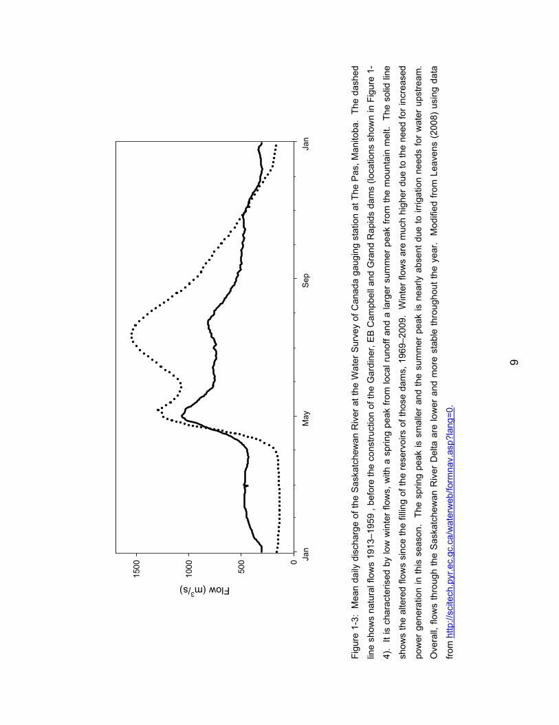
Figure 1-3: Mean daily discharge of the Saskatchewan River at the Water
Survey of Canada gauging station at The Pas, Manitoba. The dashed line
shows natural flows 1913–1959 , before the construction of the Gardiner, EB
Campbell and Grand Rapids dams (locations shown in Figure 1-4). It is
characterised by low winter flows, with a spring peak from local runoff and a
larger summer peak from the mountain melt. The solid line shows the
altered flows since the filling of the reservoirs of those dams, 1969–2009.
Winter flows are much higher due to the need for increased power
generation in this season. The spring peak is smaller and the summer peak
is nearly absent due to irrigation needs for water upstream. Overall, flows
through the Saskatchewan River Delta are lower and more stable throughout
the year. Modified from Leavens (2008) using data from
http://scitech.pyr.ec.gc.ca/waterweb/formnav.asp?lang=0. ........................... 9
Figure 1-4: The basin of the Saskatchewan River basin extends across three
provinces and into the United States. The location of the SRD is indicated
by the arrow. Cities and major towns are indicated by squares and circles.
Dams are marked by triangles. Note: Squaw Rapids Dam is currently known
as the EB Campbell Dam. Modified from Mudry (nd). ................................ 10
viii
Figure 3-1: Location of the Summerberry Marshes within the Saskatchewan
River Delta. The Saskatchewan River flows through the region; the
Summerberry River is shown to the north. Study wetlands are identified in
Figure 3-2. ................................................................................................... 25
Figure 3-2: A map of the Summerberry Marshes, with study wetlands
highlighted. Drawdown wetlands 33/35HI, 34/37C and 14R are marked in
solid black. Control wetlands 34HI, 32C, and 21C are shown with black and
white hatching. Hill Island camp is represented by the tent symbol............ 26
Figure 3-3: Summerberry water control structures. Top left: 35HI weir, viewed
from the wetland. Top right: 37C weir, viewed from the Saskatchewan
River, releasing water. Bottom left: 14R weir, viewed from the back
channel. Bottom right: 32C gated culvert control structure. Other control
wetlands had similar gated culvert controls, which were not operated during
2007 and 2008. Photography by Dale Wrubleski. ...................................... 27
Figure 3-4: Research assistants Jared Knockaert and Sheila Atchison initiate
drawdown by removing stoplogs from a Summerberry weir. ....................... 28
Figure 3-5: Monthly trends in mean maximum temperature (red), mean
temperature (black), and mean minimum temperature (blue) for summer
months at The Pas, Manitoba. Circles and solid lines represent 2007;
triangles and dotted lines represent 2008; squares and dashed lines
represent norms for the period 1971 – 2000. Data from the Canadian
Meteorological Service. ............................................................................... 29
Figure 3-6: Total monthly rainfall for summer months at The Pas, Manitoba.
Circles and solid lines represent 2007; triangles and dotted lines represent
2008; squares and dashed lines represent norms for the period 1971 –
2000. Data from the Canadian Meteorological Service. ............................. 30
ix
Figure 3-7: Monthly trends in mean daily maximum wind gust for summer
months at The Pas, Manitoba. See Figure 3-6 for legend. ......................... 30
Figure 4-1: The Summerberry Marshes, with the locations of this study's 36
wetland and two river channel sampling sites marked by white circles. ...... 38
Figure 4-2: Total nitrogen concentrations (mg/L) in each of the six study
wetlands over the summers of 2007 and 2008. Each white circle represents
the mean of open water sites (n = 3); each black circle represents the mean
of vegetated / sheltered sites (n = 3). Error bars show standard deviation.
Drawdown wetlands are on the left; control wetlands, on the right.............. 45
Figure 4-4: Ammonia concentrations (µg/L) in each of the six study wetlands
over the summers of 2007 and 2008. See Figure 4-3 for legend. .............. 46
Figure 4-3: Total nitrogen concentrations (mg/L) in control wetlands in 2007 (n =
85), control wetlands in 2008 (n = 122), drawdown wetlands in 2007 (n = 72)
and drawdown wetlands in 2008 (n = 95). Error bars show standard error.47
Figure 4-5: Ammonia concentrations (µg/L) in control wetlands in 2007 (n = 90),
control wetlands in 2008 (n = 126), drawdown wetlands in 2007 (n = 75) and
drawdown wetlands in 2008 (n = 104). Error bars show standard error. .... 47
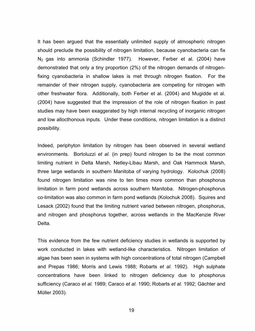
Figure 4-6: Total phosphorus concentrations (µg/L) in each of the six study
wetlands over the summers of 2007 and 2008. See Figure 4-3 for legend.48
Figure 4-8: Total reactive phosphorus concentrations (µg/L) in each of the six
study wetlands over the summers of 2007 and 2008. See Figure 4-3 for
legend.......................................................................................................... 49
x
Figure 4-7: Total phosphorus concentrations (µg/L) in all wetlands in 2007 (n =
160) and 2008 (n = 217). Error bars show standard error. ......................... 50
Figure 4-9: Total reactive phosphorus concentrations (µg/L) in control wetlands
in 2007 (n = 90), control wetlands in 2008 (n = 126), drawdown wetlands in
2007 (n = 75) and drawdown wetlands in 2008 (n = 104). Error bars show
standard error.............................................................................................. 50
Figure 4-10: Dissolved organic carbon (mg/L in each of the six study wetlands
over the summers of 2007 and 2008. See Figure 4-3 for legend. .............. 51
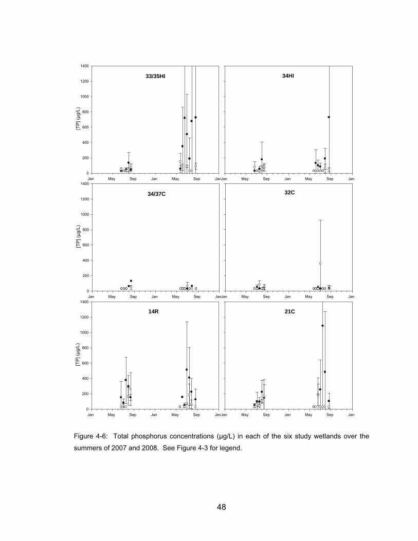
Figure 4-11: Dissolved organic carbon concentrations (mg/L) in control wetlands
in 2007 (n =102), control wetlands in 2008 (n = 125), drawdown wetlands in
2007 (n = 75) and drawdown wetlands in 2008 (n = 87). Error bars show
standard error.............................................................................................. 52
Figure 4-12: Dissolved organic carbon concentrations (mg/L) at open water sites
(n = 204) and vegetated sites (n = 185). Error bars show standard error. .. 52
Figure 4-13: Dissolved inorganic carbon concentrations (mg/L) in each of the six
study wetlands over the summers of 2007 and 2008. See Figure 4-3 for
legend.......................................................................................................... 53
Figure 4-14: Dissolved organic carbon concentrations (mg/L) in control wetlands
in 2007 (n = 84), control wetlands in 2008 (n = 126), drawdown wetlands in
2007 (n = 71) and drawdown wetlands in 2008 (n = 104). Error bars show
standard error.............................................................................................. 54
Figure 4-15: Dissolved inorganic carbon concentrations at open water sites (n =
205) and vegetated sites (n = 184) in all wetlands in 2007 and 2008. Error
bars show standard error............................................................................. 54
xi
Figure 4-16: Specific conductance in each of the six study wetlands over the
summers of 2007 and 2008. See Figure 4-3 for legend. ............................ 55
Figure 4-17: Specific conductance in control wetlands (µS/cm) in 2007 (n = 90),
control wetlands in 2008 (n = 120), drawdown wetlands in 2007 (n = 75) and
drawdown wetlands in 2008 (n = 98). Error bars show standard error. ...... 56
Figure 4-18: Specific conductance (µS/cm) at open water sites (n = 209) and
vegetated sites (n = 207) in all wetlands in 2007 and 2008. Error bars show
standard error.............................................................................................. 56
Figure 4-19: Chloride, sodium and potassium concentrations (mg/L) in control
wetlands in 2007 (n = 54), control wetlands in 2008 (n = 18), drawdown
wetlands in 2007 (n = 45) and drawdown wetlands in 2008 (n = 14). Error
bars show standard error............................................................................. 57
Figure 4-20: Magnesium and calcium concentrations (mg/L) in all wetlands in
2007 (n = 99) and 2008 (n = 32). Error bars show standard error. ............. 57
Figure 4-21: Calcium concentrations (mg/L) at open water sites (n = 68) and
vegetated sites (n = 63) in all wetlands in 2007 and 2008. Error bars show
standard error.............................................................................................. 58
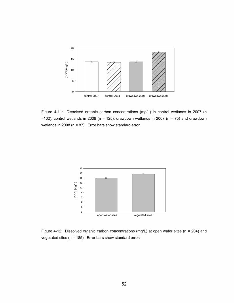
Figure 4-22: Turbidity (NTU) in each of the six study wetlands over the summers
of 2007 and 2008. See Figure 4-3 for legend. ............................................ 59
Figure 4-23: Turbidity (NTU) in control wetlands in 2007 (n = 90), control
wetlands in 2008 (n = 125), drawdown wetlands in 2007 (n = 75) and
drawdown wetlands in 2008 (n = 104). Error bars show standard error. .... 60
xii
Figure 4-24: Phytoplankton biomass, expressed as µg/L chlorophyll α, in each of
the six study wetlands over the summers of 2007 and 2008. See Figure 4-3
for legend. ................................................................................................... 61
Figure 4-25: Phytoplankton biomass, represented by chlorophyll α concentration
(µg/L), at open water sites (n = 186) and vegetated sites (n = 175) in all
wetlands in 2007 and 2008. Error bars show standard error. ..................... 62
Figure 4-26: Periphyton biomass, expressed as chlorophyll (µg/cm²), in control
wetlands in 2007 (n = 8), control wetlands in 2008 (n = 9), drawdown
wetlands in 2007 (n = 9) and drawdown wetlands in 2008 (n = 9), over a two-
week duration, on surfaces not enriched by nutrients. Error bars show
standard error.............................................................................................. 62
Figure 4-27: Periphyton biomass, expressed as chlorophyll (µg/cm²), in high
water and low water wetlands over a two-week duration. Error bars show
standard error.............................................................................................. 63
Figure 4-28: Relationships between nutrient concentration and site depth.
Clockwise from top left: total nitrogen (n = 403), total phosphorus (n = 406),
total reactive phosphorus (n = 414), and ammonia (n = 424). A minimum of
98% of points are displayed (some high concentrations at shallow depths
were outside the range of the y axis)........................................................... 70
Figure 4-29: Relationships between water quality parameters and site depth.
Clockwise from top left: dissolved organic carbon (n = 383), dissolved
inorganic carbon (n = 414), phytoplankton chlorophyll (n = 388), and turbidity
(n = 424). A minimum of 98% of points are displayed (some high
concentrations at shallow depths were outside the range of the y axis). ..... 71
xiii
Figure 4-30: Relationships between water quality parameters and site depth.
Clockwise from top left: specific conductance (n = 412), calcium ion
concentration (n = 139), magnesium ion concentration (n = 139), and sodium
ion concentration (n = 139). A minimum of 98% of datapoints are displayed
(some high concentrations at shallow depths were outside the range of the y
axis)............................................................................................................. 72
Figure 4-31: Total nitrogen concentrations (mg/L) in the Saskatchewan River (n
= 11) and the back channel (n = 11) in 2007 and 2008. Error bars show
standard error.............................................................................................. 75
Figure 4-32: Total nitrogen concentrations (mg/L) in the back channel in 2007(n
= 5) and 2008 (n = 6). Error bars show standard error. .............................. 75
Figure 4-33: Total phosphorus concentrations (µg/L) in the Saskatchewan River
(n = 11) and the back channel (n = 11) in 2007 and 2008. Error bars show
standard error.............................................................................................. 76
Figure 4-34: Total phosphorus concentrations (µg/L) in the Saskatchewan River
in 2007(n = 5) and 2008 (n = 6). Error bars show standard error. .............. 76
Figure 4-35: Total reactive phosphorus concentrations (µg/L) in the
Saskatchewan River (n = 12) and the back channel (n = 12) in 2007 and
2008. Error bars show standard error......................................................... 77
Figure 4-36: Dissolved organic carbon concentrations (mg/L) in all wetland sites
(n = 389) and the channel sites (Saskatchewan River and back channel), (n
= 21) in 2007 and 2008. Error bars show standard error............................ 78
Figure 4-37: Dissolved organic carbon concentrations (mg/L) at channel sites in
2007 (n = 10) and 2008 (n = 11). Error bars show standard error. ............. 78
xiv
Figure 4-38: Dissolved inorganic carbon concentrations (mg/L) in all wetland
sites (n = 419) and the channel sites (Saskatchewan River and back
channel), (n = 24) in 2007 and 2008. Error bars show standard error. ....... 79
Figure 4-39: Concentrations of chloride, sodium and potassium (mg/L) at all
channel sites (Saskatchewan River and back channel) in 2007 (n =6) and
2008 (n = 2). Error bars show standard error. ............................................ 79
Figure 4-40: Turbidity (NTU) in all wetland sites (n = 430) and the channel sites
(Saskatchewan River and back channel, (n = 24) in 2007 and 2008. Error
bars show standard error............................................................................. 80
Figure 4-41: Turbidity (NTU) in the Saskatchewan River (n = 12) and the back
channel (n = 12) in 2007 and 2008. Error bars show standard error. ......... 80
Figure 4-42: Euphotic depth (cm), in the Saskatchewan River (n = 9) and the
back channel (n = 9) in 2007 and 2008. Error bars show standard error.... 81
Figure 4-43: Euphotic depths (cm) in the back channel in 2007(n = 4) and 2008
(n = 5). Error bars show standard error. ..................................................... 81
Figure 4-44: Periphyton biomass, expressed as chlorophyll (µg/cm²), in wetlands
(n = 35) and channels (n = 12), over two-week durations in 2007 and 2008.
Error bars show standard error.................................................................... 82
Figure 4-45: Periphyton biomass, expressed as chlorophyll (µg/cm²), in the
Saskatchewan River (n = 6) and the back channel (n = 6), over two-week
durations in 2007 and 2008. Error bars show standard error. .................... 82
Figure 4-46: The relationship between wetland water column ammonia
concentration (µg/L) and distance from the nearest channel (n = 431). ...... 85
xv
Figure 4-47: The relationship between dissolved organic carbon concentration
(mg/L) and distance from the nearest channel (n = 389)............................. 85
Figure 4-48: The relationship between magnesium concentration (mg/L) and
distance from the nearest channel (n = 108). .............................................. 86
Figure 4-49: The relationship between sediment water content and sediment
density. ........................................................................................................ 89
Figure 4-50: The relationship between sediment water content and sediment
organic content............................................................................................ 90
Figure 4-51: The relationships between water content and organic content of
wetland sediment, and the distance from the Saskatchewan River (n = 96).
Filled circles represent water content; open circles represent organic
content......................................................................................................... 90
Figure 4-52: The relationship between wetland wet sediment density and the
distance from the Saskatchewan River (n = 102). ....................................... 91
Figure 4-53: The relationship between total phosphorus concentration (µg/gww)
in wetland sediment and distance from the Saskatchewan River (n = 37). . 91
Figure 4-54: The relationship between the concentration of total nitrogen (mg/L)
in the wetland water column and the sediment water content at
corresponding sites (n = 93)........................................................................ 92
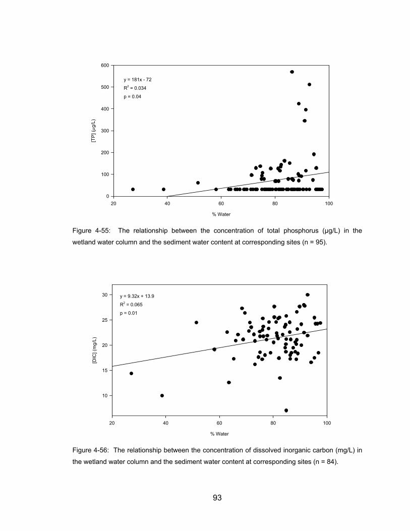
Figure 4-55: The relationship between the concentration of total phosphorus
(µg/L) in the wetland water column and the sediment water content at
corresponding sites (n = 95)........................................................................ 93
xvi
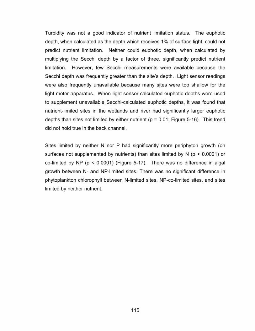
Figure 4-56: The relationship between the concentration of dissolved inorganic
carbon (mg/L) in the wetland water column and the sediment water content
at corresponding sites (n = 84). ................................................................... 93
Figure 4-57: The relationship between dissolved inorganic carbon (mg/L) in the
water column and sediment total nitrogen concentrations (mg/L) (n = 76). . 94
Figure 4-58: The relationship between phytoplankton biomass, as approximated
by chlorophyll α concentration (µg/L) in the water column and sediment total
nitrogen concentrations (n = 76).................................................................. 94
Figure 4-59: The relationship between calcium and magnesium concentrations
(mg/L) and sediment water content. Filled circles represent calcium; open
circles represent magnesium (n =96). ......................................................... 95
Figure 4-60: The relationship between specific conductance (µS/cm) and
sediment water content (n = 93). ................................................................. 95
Figure 5-1: Nutrient diffusing substratum consisting of a plastic tube filled with
nutrient enriched agar and capped with a silica frit. The frit is being
removed, to be frozen for a methanol extraction of periphyton chlorophyll.
.................................................................................................................. 108
Figure 5-2: The author removing a floating NDS frame, holding 16 randomly
arranged vials of four nutrient agar treatments, after its deployment in the
marsh for a period of two weeks................................................................ 109
Figure 5-3: A floating frame containing NDS vials, deployed at a marsh site. . 110
xvii
Figure 5-4: Six potential NDS outcomes: a) ns: no significant treatment effect (no
treatment has significantly more algal growth than any other), b) NP:
nitrogen and phosphorus co-limitation (the N and P combined treatment has
significantly more growth), c) N: nitrogen limitation (the N alone and NP
treatments have significantly more growth), d) N: nitrogen limitation (the N
alone treatment has significantly more growth), e) P: phosphorus limitation
(the P alone and NP treatments have significantly more growth), or f) P:
phosphorus limitation (the P alone treatment has significantly more growth).
.................................................................................................................. 111
Figure 5-5: A sample periphyton growth response to the four NDS treatments.
Clockwise from top left: control agar, agar enriched with N, agar enriched
with N and P, agar enriched with P. .......................................................... 112
Figure 5-6: The most common response to NDS was NP-colimitation. Clockwise
from top left: control treatment; N treatment; N + P treatment, showing a
dramatic periphyton response; P treatment............................................... 116
Figure 5-7: Distribution of the limitation status of all sites in which NDS
experiments were conducted over 2007 and 2008. Wetlands sites (n = 35)
are shown separately from the back channel (n = 6) and Saskatchewan
River sites (n = 6). N indicates N-limitation, NP indicates NP co-limitation,
and ns indicates no significant limitation by either nutrient (p > 0.05).
Results are presented although there was no statistically significant
difference between wetlands, back channel and river by ChiSquare analysis.
.................................................................................................................. 117
xviii
Figure 5-8: The magnitude of the treatment effect of nutrient enrichment on
periphyton, relative to the control, in Summerberry wetlands (n = 27), in the
back channel (n = 5) and in the Saskatchewan River (n = 3), including both
N- and NP-limited sites. The relative treatment effect in the river is
significantly lower than that in the back channel (p = 0.02), but neither differs
significantly from the wetlands................................................................... 117
Figure 5-9: Distribution of the limitation status of wetlands in 2007 (n = 17) and
2008 (n = 18) was significantly different (p = 0.002; RSquare = 0.201). See
Figure 5-7 for legend. ................................................................................ 118
Figure 5-10: Distribution of the limitation status of high-water wetlands (all
wetlands in 2007 plus control wetlands in 2008; n = 24) and drawdown
wetlands (in 2008; n = 9) was significantly different (p = 0.0002; RSquare =
0.263). See Figure 5-7 for legend............................................................. 118
Figure 5-11: Distribution of the limitation status of control wetlands (n = 9) and
drawdown (n = 9) wetlands in 2008 was significantly different (p = 0.003;
RSquare = 0.361). See Figure 5-7 for legend. ......................................... 119
Figure 5-12: Distribution of the limitation status of the experimental wetlands in
the pre-drawdown season of 2007 (n = 9) and the same wetlands during
drawdown in 2008 (n = 9) was significantly different (p = 0.0004; Rsquare =
0.447). See Figure 5-7 for legend............................................................. 119
Figure 5-13: Total nitrogen concentrations (mg/L) at nutrient-limited sites (n =
26) and sites limited by neither nitrogen nor phosphorus (n = 9). Error bars
represent standard error............................................................................ 120
xix
Figure 5-14: Dissolved organic carbon (mg/L) at nutrient-limited sites (n = 26)
and sites limited by neither nitrogen nor phosphorus (n = 9). Error bars
represent standard error............................................................................ 120
Figure 5-15: Total carbon (mg/L) to total nitrogen molar ratios at N-limited sites
(n = 5), NP-co-limited sites (n = 21) and sites limited by neither nitrogen nor
phosphorus (n = 9). Error bars represent standard error.......................... 121
Figure 5-16: Mean euphotic depths (m) at nutrient-limited (N-limited or NP-co-
limited; n = 20) and non nutrient-limited sites (n = 3) in the wetlands and
river. .......................................................................................................... 121
Figure 5-17: Periphyton biomass, expressed as chlorophyll (µg/cm²), in N-limited
wetlands (n = 22), NP-co-limited wetlands (n = 112), and wetlands limited by
neither N nor P (n = 46), over two-week durations in 2007 and 2008, on
surfaces not enriched by nutrients............................................................. 122
Figure 6-1: Research assistant Sheila Atchison harvesting aboveground
vegetation from a quadrat in a whitetop / sedge / horsetail stand.............. 130
Figure 6-2: Research assistants Martin Blades and Jared Knockaert sampling
submersed vegetation from a barrel in a drawdown wetland..................... 131
Figure 6-3: The root coring device with a below-ground biomass sample.
Photography by Dale Wrubleski. ............................................................... 132
Figure 6-4: The automatic root washing machine. A submersible pump in the
river forced water into the grey tub through the white hose in the foreground.
An electric motor (right) caused the wire mesh cylinder to rotate. Root cores
were placed in the four separate cages within the cylinder. Dirty water
drained through the hose at the rear. ........................................................ 133
xx
Figure 6-5: Cattails in the Summerberry Marshes. From left: Typha latifolia,
native common cattail; T. X glauca, hybrid cattail, exhibiting characteristics
of both parents; T. angustifolia, introduced narrow-leaved cattail.............. 138
Figure 6-6: Mean aboveground biomass in stands of phragmites (n = 28), cattail
(n = 33), bulrush (n = 19), sedge (n = 24), and submersed vegetation (n =
53). Error bars show standard error (n = 157). ......................................... 139
Figure 6-7: Phragmites stands (top) and bulrush stands (bottom) in the
Summerberry Marshes exhibited monodominance. .................................. 140
Figure 6-8: Some examples of the variability of composition of sedge stands,
including (clockwise from top left) sedge dominant with horsetail present;
horsetail dominant with sedge present; sedge, horsetail and whitetop grass
present; whitetop grass dominant with sedge present............................... 141
Figure 6-9: Several examples of the variability of species composition in stands
of submersed and floating-leaved plants. .................................................. 142
Figure 6-10: Mean belowground biomass in stands of Phragmites (n = 32),
cattail (n = 24), bulrush (n = 30), and sedge (n = 30). Error bars show
standard error (n = 116). ........................................................................... 143
Figure 6-11: Utricularia vulgaris. High densities of Utricularia spp. were observed
in small patches of open water amongst emergent vegetation; lower
densities were sampled from large open bays. ......................................... 148
xxi
List of Tables
Table 3-1: Characteristics describing Summerberry study wetlands. Basin areas
from Clay (1978).......................................................................................... 31
Table 3-2: Original and target water levels for drawdown wetlands, and the date
drawdown commenced and completed. The largest wetland, 37C, did not
fully drain to target level in early fall 2007, so drawdown was reinitiated in
spring 2008. 34C never reached the target water level. ............................. 32
Table 3-3: Climate parameters for June – July – August 2007 and 2008 at
Environment Canada’s The Pas airport weather station. Normals for the
period 1971 – 2000 are also presented. 2008 was the warmer, drier, windier
year. Both 2007 and 2008 were warmer and much drier than the normals.32
Table 4-1: Dates of the five rounds of water sampling in 2007 and the seven
rounds in 2008............................................................................................. 38
Table 4-2: Methods used for water chemistry analyses..................................... 39
Table 4-3: Formulae for calculation sediment composition parameters by loss on
ignition. ........................................................................................................ 63
Table 4-4: Mean sodium concentrations (mg/L) in open water sites and
vegetated / sheltered sites in summers 2007 and 2008 ± standard deviation.
.................................................................................................................... 64
Table 4-5: Mean potassium concentrations (mg/L) in open water sites and
vegetated / sheltered sites in summers 2007 and 2008. ............................. 65
xxii
Table 4-6: Mean calcium concentrations (mg/L) in open water sites and
vegetated / sheltered sites in summers 2007 and 2008. ............................. 66
Table 4-7: Mean magnesium concentrations (mg/L) in open water sites and
vegetated / sheltered sites in summers 2007 and 2008. ............................. 67
Table 4-8: Mean chloride concentrations (mg/L) in open water sites and
vegetated / sheltered sites in summers 2007 and 2008. ............................. 68
Table 4-9: Water quality in the Saskatchewan River and Back Channel. Mean
values for each parameter are presented, with the range from minimum and
maximum shown below. .............................................................................. 83
Table 4-10: Parameters describing the relationship between major ions and
distance from the nearest channel (n = 108). The relationship between
conductivity and distance from the nearest channel is also included (n =
105). ............................................................................................................ 86
Table 4-11: Mean values of sediment composition parameters ± standard
deviation. nm = not measured. .................................................................... 89
Table 4-12: The minimum wind speed required for wave action to resuspend
sediments at a hypothetical but typical Summerberry site (fetch = 150 metres
across a circular pond; effective fetch = 54.4m), given various water depths.
The percentage of days from May to September 2007 and 2008 on which
that minimum wind velocity was reached is also listed. ............................. 100
xxiii
Table 4-13: A comparison of water quality parameters between the
Summerberry Marshes and other Manitoba and boreal wetlands.
Summerberry values are 2007 only. Delta Marsh values from Goldsborough
(unpublished data). Netley-Libau and Oak Hammock Marshes (1997)
values from Bortoluzzi et al. (in prep). PAD values estimated from figures in
Wolfe et al. (2007). Northern Alberta boreal lakes values from Bayley and
Prather (2003). .......................................................................................... 103
Table 6-1: Major plant species observed in the Summerberry region, with
scientific and common nomenclature according to Laring (2003). A cross (†)
precedes those species which were present in vegetation samples. An
asterisk (*) precedes the most abundant member of a genus where more
than one species was present. .................................................................. 144
Table 6-2: The percentage of the total biomass which was comprised of the
stand’s type vegetation. The means, standard errors, and minimums are
presented for each stand type: bulrush (n = 19), cattail (n = 33) and
phragmites (n = 28). .................................................................................. 145
Table 6-3: The makeup of a sedge stand: biomass of sedge, horsetail and
whitetop grass within Sedge etc stands. ................................................... 145
Table 6-4: Biomass of submersed plants and the percentage of sites where
genera was present. .................................................................................. 146
Table 6-5: Percentage of the total (above- plus below-ground) biomass of
emergent vegetation that is aboveground, or the shoot to root ratio. ........ 146
xxiv
Table 6-6: A comparison of above-ground macrophyte biomass (g/m2, and
percent of biomass which is above-ground) between the Summerberry
Marshes, Delta Marsh (Shay and Shay 1986) and Eagle Lake Marsh (van
der Valk and Davis 1978b). ....................................................................... 149
1
Chapter 1: Introduction
Background
The ecology of Canada’s prairie wetlands has been well described, on scales
ranging from short-term descriptive studies (Weller and Fredrickson 1974; van
der Valk and Davis 1978a; an der Valk and Davis 1978b) to decade-long
interdisciplinary whole ecosystem manipulation projects (Murkin et al. 2000). It
has been well-established that a fluctuating water regime is the major driver of
prairie marsh dynamics. By contrast, wetland ecology in boreal Canada has
been poorly studied, and the response of northern marshes to variations in water
levels is thus far unknown.
Boreal Wetlands and Deltaic Marshes
The boreal region encompasses one third of the area of Canada, and of this
area, wetlands comprise approximately 20% or over 600,000 km2 (National
Wetlands Working Group 1988). The majority of these are peatlands, but there
are significant areas of marshes along the shores of lakes and in the deltas
formed as rivers discharge into large lakes. Older portions of deltas, less
frequently subjected to river floods, have often developed into fens, bogs and
treed swamps (Dirschl 1972b). However, in the active portions of deltas nearer
to the developing margin, marshes and shallow open water can be found behind
river channel levees. The larger boreal delta marshes include the Slave River
Delta, the Peace-Athabasca Delta, and, largest of all, the Saskatchewan River
Delta.
Saskatchewan River Delta
The Saskatchewan River Delta (SRD) is an inland delta in the Mid-Boreal
Lowlands ecoregion of the Boreal Plains ecozone. The delta has been forming
2
since the late Holocene with sediments deposited by the Saskatchewan River as
it entered glacial Lake Agassiz and its remnant plain and lakes (Morozova and
Smith 2003). The SRD now consists of over 9000 km2 (National Wetlands
Working Group 1888) of wetlands, shallow lakes, and active and abandoned river
channels bordered by forested natural levees (Morozova and Smith 2003), in
eastern central Saskatchewan and western central Manitoba (Figures 1-1 and 1-
2). The larger, older Upper Delta is divided from the younger, more active Lower
Delta by the moraine at The Pas, Manitoba. Together, the upper and lower
portions of the SRD comprise the largest freshwater inland river delta in North
America (Wrubleski 2008).
The SRD is home to 13,000 people (Smith 2008), in communities including The
Pas, Opaskwayak Cree Nation, and Cumberland House, or isolated in remote
areas. The delta is also home to myriad plants and animals. Fur-bearing
mammals, especially beaver and muskrat, but also mink, otter, fisher, and lynx,
have been and are an important resource to local trappers (McLeod et al. 1947;
Uchtmann 2008). Large mammals, including moose, black bear, elk, wolf, and
deer, provide tourism revenue from southern hunters, a source of food for local
hunters, and opportunities for wildlife viewing (Smith 2008). The SRD has been
designated an Important Bird Area nationally (Poston et al. 1990) and
internationally (Partners FOR the Saskatchewan River Basin 2008). Over 120
species of birds are found in the delta (Smith 2008), including nearly 500,000
ducks (Slattery 2008). Open water areas in the delta provide habitat for 48
species of fish (Rosenberg et al. 2005), including commercially important species
like walleye and recreationally important species like northern pike. Species
important to the bait fishery, such as shiners, and species at risk, including the
lake sturgeon, are also represented.
Over the last century, the SRD has been increasingly impacted by upstream and
downstream development. Upstream of the delta, hydroelectric projects have
combined with increased agricultural irrigation demands on the Saskatchewan
3
River to dramatically alter its hydrology (Figure 1-3). Nineteen dams have been
constructed on the Saskatchewan River or its tributaries (Partners FOR the
Saskatchewan River Basin 2008), most notably the EB Campbell, less than 100
km upstream of the SRD, and the Gardiner, on the South Saskatchewan River
(Figure 1-4). These dams change downstream patterns of annual flow by
retaining water during high flows and releasing it during traditionally low flow
periods (Leavens 2008). Annually, 10 to 20% of the Saskatchewan River’s
naturalised flow is consumed upstream of the SRD, partly to support an area of
5000 km2 of irrigated agriculture (Partners FOR the Saskatchewan River Basin
2008). The diminished, stabilised river flows have reduced the probability of
flooding to permanently separated wetland basins from once in ten years to once
in fifty years (Leavens 2008).
Changes in river water quality also have impacts on the SRD. The drainage
basin of the Saskatchewan River encompasses 420,000 km2 of Montana,
Alberta, Saskatchewan, and Manitoba and is home to three million people
(Partners FOR the Saskatchewan River Basin 2008). Agricultural activity is
prevalent in much of this region – as much as 90% of land within the South
Saskatchewan River sub-basin is cropland or rangeland (Saskatchewan
Watershed Authority 2007), and agricultural runoff can be a non-point source of
nutrients and pollutants (Cooke and Prepas 1998). The many towns and several
major urban areas, including Calgary, Edmonton, Saskatoon and Lethbridge,
through which the river and its tributaries pass (Figure 1-4) may be point sources
of pollutants. Non-urban industrial activity within the watershed, including
extraction and processing of forestry, mining, and petrochemical resources, may
also change water quality in the delta (Partners FOR the Saskatchewan River
Basin 2008).
Finally, the SRD has lost substantial wetland area through flooding and drainage.
The hydroelectric dam at Grand Rapids, Manitoba downstream of the SRD,
permanently flooded more than 1000 km2 of the lower delta (Uchtmann 1983),
4
and the Pasquia land reclamation project drained 550 km2 of wetlands in the
Carrot River Valley, west of The Pas, Manitoba, for farmland in the 1950s
(Partners FOR the Saskatchewan River Basin 2008). These changes to the
SRD have been noted by local trappers and hunters, who have described
marked declines in the resources they extract from the SRD, most particularly in
muskrats (Uchtmann 2008) and ducks (Slattery 2008).
Despite the size and importance of the SRD and the threats it is facing, the
ecological function of the delta has been relatively unstudied. Qualitative
information is available, in the form of traditional ecological knowledge from area
residents, and descriptions of annual wetland monitoring conducted by Ducks
Unlimited Canada, but scientific studies have been limited. Some of the earliest
descriptions were written by McLeod (1947), who, very qualitatively, described
vegetation and water quality as they related to muskrat production. Dirschl and
colleagues (Dirschl and Dabbs 1969; Dirschl 1970; Dirschl 1972b; Dirschl and
Coupland 1972) described several vegetation assemblages within wetlands of
the upper SRD, and studied vegetation succession pathways. Ducks Unlimited
visits many wetlands within the SRD yearly to observe waterbirds and habitat,
but data in their reports tend to be qualitative and to vary in content from year to
year. More recently, Morozova and Smith (2003) have described the
development of the delta by studying its progradation, avulsion and other fluvial
sedimentary processes, mainly in the upper delta.
Objectives
In response to concerns raised by local resources users over the health of the
SRD ecosystem and an overall lack of knowledge relating to the ecology of
boreal deltaic wetlands, a multi-faceted ecological study was conceived by Ducks
Unlimited Canada scientists at the Institute for Wetlands and Waterfowl
Research. This study would investigate populations of muskrats, fish, waterfowl
and other waterbirds within the SRD, and, because the decline in animal
5
populations was suspected to be result of habitat deterioration, perhaps because
of long-term water level stabilisation, it was also deemed useful to study water
quality and primary production in SRD wetlands.
The study proposed to address habitat concerns and these objectives by
monitoring the responses of the aforementioned populations to experimental
water level manipulation, with the objective of informing future wetland
management practices. These water level manipulations were designed to
mimic the natural fluctuations of the SRD, which have been disrupted in recent
years. The study, modeled on the Marsh Ecology Research Project (Murkin et
al. 2000), was designed as a drawdown and reflood project, in which wetland
water levels would be experimentally lowered, then, after several years, raised.
Within the context of this larger study, this research project specifically strove to
achieve three objectives:
• Describe the water quality and vegetation community of the SRD, a largely
unstudied northern deltaic wetland.
• Understand the effects of lowering water levels on water quality and algal
primary production.
• Suggest strategies to control wetland water quality and primary production
by water manipulation that may be useful for managing fish and wildlife
communities.
Hypotheses
A. Drawdown will affect water quality by increasing water column turbidity
and nutrient concentrations because shallower water allows for more
sediment – water mixing by wind.
6
B. Increases in nutrient concentration due to drawdown will increase algal
primary production, because algal communities in deltaic wetlands, like
those in many prairie wetlands, are nutrient limited.
C. Turbidity, nutrient concentrations and algal primary production trends will
be related to site depth because sediment resuspension is more likely to
occur in shallow sites. Shallow sites in wetland basins not undergoing a
drawdown should therefore be similar to drawdown sites in these
parameters.
D. The chemical and physical properties of wetland water and sediment will
be correlated to distance from channels of the Saskatchewan River,
because the river influences wetlands through flood events and seepage
through levees.
7
Figu
re 1
-1: L
ocat
ion
of th
e S
aska
tche
wan
Riv
er D
elta
in w
este
rn c
entra
l Sas
katc
hew
an a
nd e
aste
rn c
entra
l Man
itoba
, Can
ada.
Th
e m
ajor
riv
er
chan
nels
and
som
e la
rge
lake
s ar
e sh
own.
8
Figu
re 1
-2:
Sat
ellit
e im
age
show
ing
SR
D fe
atur
es in
clud
ing
wet
land
s, s
hallo
w la
kes,
act
ive
and
aban
done
d riv
er c
hann
els
and
natu
ral l
evee
s.
Mod
ified
from
Sm
ith (2
008)
.
9
Jan
M
ay
Sep
Ja
n
Flow (m3/s)
0
500
1000
1500
Figu
re 1
-3:
Mea
n da
ily d
isch
arge
of t
he S
aska
tche
wan
Riv
er a
t the
Wat
er S
urve
y of
Can
ada
gaug
ing
stat
ion
at T
he P
as, M
anito
ba.
The
dash
ed
line
show
s na
tura
l flo
ws
1913
–195
9 , b
efor
e th
e co
nstru
ctio
n of
the
Gar
dine
r, E
B C
ampb
ell a
nd G
rand
Rap
ids
dam
s (lo
catio
ns s
how
n in
Fig
ure
1-
4).
It is
cha
ract
eris
ed b
y lo
w w
inte
r flo
ws,
with
a s
prin
g pe
ak fr
om lo
cal r
unof
f and
a la
rger
sum
mer
pea
k fro
m th
e m
ount
ain
mel
t. T
he s
olid
line
show
s th
e al
tere
d flo
ws
sinc
e th
e fil
ling
of th
e re
serv
oirs
of t
hose
dam
s, 1
969–
2009
. W
inte
r flo
ws
are
muc
h hi
gher
due
to th
e ne
ed fo
r inc
reas
ed
pow
er g
ener
atio
n in
this
sea
son.
Th
e sp
ring
peak
is s
mal
ler
and
the
sum
mer
pea
k is
nea
rly a
bsen
t due
to ir
rigat
ion
need
s fo
r w
ater
ups
tream
.
Ove
rall,
flow
s th
roug
h th
e S
aska
tche
wan
Riv
er D
elta
are
low
er a
nd m
ore
stab
le th
roug
hout
the
year
. M
odifi
ed fr
om L
eave
ns (
2008
) us
ing
data
from
http
://sc
itech
.pyr
.ec.
gc.c
a/w
ater
web
/form
nav.
asp?
lang
=0.
10
Figu
re 1
-4:
The
basi
n of
the
Sas
katc
hew
an R
iver
bas
in e
xten
ds a
cros
s th
ree
prov
ince
s an
d in
to th
e U
nite
d S
tate
s.
The
loca
tion
of th
e S
RD
is
indi
cate
d by
the
arro
w.
Citi
es a
nd m
ajor
tow
ns a
re in
dica
ted
by s
quar
es a
nd c
ircle
s. D
ams
are
mar
ked
by tr
iang
les.
Not
e: S
quaw
Rap
ids
Dam
is
curre
ntly
kno
wn
as th
e E
B C
ampb
ell D
am.
Mod
ified
from
Mud
ry (n
d).
11
Chapter 2: Literature Review
Effect of water level variation on nutrients, algae, and macrophytes
The drought of the 1930s contributed to a basic understanding of the effects that
water level variation could have on wetland ecosystem function. A variety of
descriptive research was undertaken over the next decades (Bourn and Cottam
1939; Walker 1959; Kadlec 1962; Walker 1965; Weller and Spatcher 1965; Smith
1971; Stout 1971; Millar 1973; Weller and Fredrickson 1974; van der Valk and Davis
1978a), but by the late 1970s, there were calls for long-term multidisciplinary
experimentation by water level manipulation to better understand wetland ecological
function (Weller 1978).
In response to this challenge, the Marsh Ecology Research Program (hereafter
referred to as MERP) was initiated in 1979 by Ducks Unlimited Canada and the
Delta Waterfowl and Wetlands Research Station. MERP was a ten year study
conducted in ten artificially constructed experimental wetland cells within Delta
Marsh, a large lacustrine wetland in Manitoba. Water chemistry, primary production,
invertebrate populations, and avian and mammal use was monitored to examine
changes ensuing from water level manipulation simulating a natural wet-dry cycle.
Over one hundred publications resulted from MERP, including the definitive text
Prairie Wetland Ecology (Murkin et al. 2000). The effects of water level manipulation
on nutrient dynamics and primary production as determined through MERP and its
predecessors will be summarised here.
Wetlands are dynamic ecosystems, subject to natural fluctuations of water level.
Prolonged flooding of a prairie wetland results in a lake marsh state, where
emergent macrophytes die back from open water bays and are unable to germinate
from the seed bank (van der Valk and Davis 1978a). Without emergent
macrophytes to take up nutrients from the sediment, and contribute to mineralisation
12
of organic matter by aerating sediments, nutrients become locked up in the sediment
and porewater pools. The decline in macrophytes also leads to a decline in litter as
available substrata for colonisation by periphyton, and as a source of nutrients to
aboveground nutrient pools through leaching and decomposition. Phytoplankton is
the dominant algal assemblage, but overall primary production from macrophytes
and algae is low in the lake marsh state because nutrients are sequestered in the
sediment and porewater.
A lowering of water levels, whether naturally through drought or through artificial
management, is termed drawdown. Drawdown allows for aeration of the sediments,
which increases microbial aerobic decomposition of organic material into inorganic
nutrients. Drawdown also allows for the germination of emergent macrophytes, such
as bulrush (Scirpus acutus and S. validus), cattail (Typha latifolia, T. angustifolia,
and T. (X) glauca), phragmites (Phragmites australis) and whitetop (Scholochloa
fesucacea), the growth of which is fuelled by these newly mineralised nutrients.
MERP found that environmental conditions, competition, herbivory and seed
dispersal are interacting factors which determine species distribution (van der Valk
2000). For example, seed germination was not greatest where seed densities for a
particular species were highest, but rather where moisture, temperature, and salinity
requirements were most suitable. Drawdown also allows annual terrestrial plants to
become established on newly exposed mudflats, which can account for more than
half of wetland above-ground biomass (van der Valk 2000).
With reflooding, the emergent vegetation again provides a pathway for taking up
sediment nutrients and transferring them to the water column and other
aboveground nutrient pools. Those annual plant species which cannot tolerate
flooding die back and their decomposition generates a pulse of nutrients released to
the water column. Epiphyton and metaphyton are the dominant algal assemblages
at this stage and production is high in response to increased nutrient availability.
Some key findings of MERP were related to the elucidation of the important role
13
played by algae in the productivity and function of prairie wetlands. High algal
productivity and rapid turnover mean that annual algal production can exceed that of
macrophytes, though the standing crop at any one point in time may be lower
(Robinson et al. 2000). MERP found that algae may play a bigger role than
macrophytes or detritus in feeding secondary productivity (Neill and Cornwell 1992;
Robinson et al. 2000), and they provide wetland invertebrates with food and
structural habitat (Murkin and Ross 2000; Robinson et al. 2000).
Although MERP was the definitive research program on the effects of water level
variation on wetland ecosystem structure and function, MERP, and indeed, the
earlier contributions to understanding the wet-dry cycle (Weller and Spatcher 1965;
Weller and Fredrickson 1974; van der Valk and Davis 1978a) took place in prairie
wetlands. Boreal wetlands require further study to elucidate their response to water
level variation.
Boreal wetlands and water level variation
The boreal region encompasses one third of the area of Canada, and of this area,
wetlands comprise approximately 20% or over 600,000 km2 (National Wetlands
Working Group 1988). The vast majority of these are peatlands: wetlands which
have a 40cm or greater layer (Tarnocai 1980) of undecomposed organic material.
Canada’s boreal region supports at least ten forms (National Wetlands Working
Group 1988) of fens, minerotrophic peat-producing wetlands with a groundwater
connection, and bogs, ombrotrophic peat-producing wetlands receiving water only
from precipation (National Wetlands Working Group 1997). Swamps, treed wetlands
not producing a peat layer, are uncommon, and marshes, non-peat-producing,
untreed wetlands, and shallow open waters, with a depth less than two metres, are
rare (N National Wetlands Working Group 1988). Those marshes and shallow open
waters that are present in boreal region are typically found either on the margins of
lakes, or in the deltas of rivers discharging into lakes or lacustrine plains (National
Wetlands Working Group 1988).
14
Because peatlands overwhelmingly dominate the boreal region – over 85% of
Canada’s wetlands are peatlands (National Wetlands Working Group 1988) – it is
not surprising that peatlands also dominate the literature relating to boreal wetlands
(Dirschl 1972b; Zoltai and Johnson 1987; Futyma and Miller 1986; Kubiw et al. 1989;
Miller and Futyma 1987; Nicholson 1993; Moore et al. 1998; Nicholson et al. 2006;
Talbot et al. 2010), while marshes and shallow open waters have received less
attention. Indeed, Bayley and Prather (2003) have lamented the lack of attention
received by shallow boreal wetland lakes.
Peatlands and non-peat-producing wetlands are not discrete entities, however.
Rather, they are different stages along successional pathways. One successional
progression, from shallow open water to fen to bog has been well documented
(Tallis 1983; Kratz and DeWitt 1986; National Wetlands Working Group 1988;
Nicholson and Witt 1994). In the process of terrestrialisation, an open water basin
develops into a fen as it becomes filled by sediments settling to the bottom and by
floating mats of vegetation, including mosses, enclosing from the basin’s periphery.
As more peat is deposited, the wetland surface may rise above the water table and
develop into a bog.
Another potential succesional pathway may be followed in regions of fluctuating
water levels. Where periodic drying can prevent the colonisation of bryophytes, an
open water basin may succeed to a marsh rather than a fen/bog. If drying is
ongoing, trees can invade and the marsh can develop into a swamp (Glooschenko
and Grondin 1988; Nicholson 1993; Nicholson and Witt 1994). If water level
fluctuations continue to include periodic flooding, the wetland remains a marsh
(Nicholson and Witt 1994).
Succession in deltaic boreal wetlands also follows these two successional pathways.
Dirchl et al. (1974) studied successional trends in the Peace-Athabasca Delta. They
are differentiated by successional pathways in inactive portions of the delta, where
15
basins receive spring floodwaters only rarely in the highest water years, and active
or semi-active areas of the delta, which are directly affected by hydrological
interactions with the river or lake, or which are recharged by floodwaters in most
years. Autogenic succession and terrestrialisation was observed in inactive parts of
delta, which had become bogs. Allogenic succession, where aquatic communities
developed into shore communities, to meadow communities, to shrub communities,
and eventually to forest communities, was observed in the active and semi-active
delta.
In non-deltaic boreal peatlands, the vegetation community has been found to be
most correlated with water flow and cation gradients; nitrogen and phosphorus
concentrations are less important in determining species composition (Nicholson
1995). In deltaic wetlands, however, nutrients seem to be more important. Dirschl
and Coupland (1972) and Dirschl (1972a) found that plant species distribution in the
upper Saskatchewan River Delta depends on moisture regime, nutrient status, and
pH. Nutrient availability and pH decrease with increasing distance from the river
along transects from mixed forest alluvial levees, to open drainage basins with
marsh or fen vegetation, to closed drainage basins with bog communities.
These studies of water level related change in deltas and other boreal wetlands
have thus far been mainly concerned with successional changes over the long-term:
hundreds or thousands of years. While studying the Saskatchewan River Delta,
Dirschl (1970) stated that “compared to the rapid, cyclic changes evident in the
wetland vegetation of the neighbouring aspen grove and grassland regions, the
vegetation changes in the study area are slower, less fluctuating, and essentially
unidirectional.” However, relatively recent changes to the water regime of the
Peace-Athabasca Delta (PAD) demonstrated that short-term effects on water quality
and vegetation can also be observed in deltaic boreal wetlands.
Prior to construction of the WAC Bennett Dam built in 1967 on the Peace River, an
annual summer flood of the Peace River would normally cause a rapid rise in water
16
level on Lake Athabasca and connected wetlands with the delta, and flooding of
isolated wetland basins (Dirschl 1972b). Since the dam interrupted this summer
flood, water levels dropped substantially on Lake Athabasca and the inundated area
of connected wetland lakes decreased by 38%, exposing 500 km2 of mudflat
(Jaques 1990). Isolated wetland basins on the floodplain have dried out partially or
completely without overbanking in flood years. The wetlands changed, over a four
year period, from marshes and shallow open waters, to open mudflats with scattered
seedlings of emergent macrophytes, to mixed communities of sedges and grasses,
to immature fens with a variety of herbaceous plants, to dense monospecies sedge
meadows, and finally were colonised by willows (Dirschl et al. 1974). This
progression was interpreted as an acceleration of the natural successional pathway
of the PAD wetlands, shifting quickly from shallow marsh and wet meadow to shrub
and forest communities, with an overall reduction in biodiversity and area and
number of wetlands (Dirschl et al. 1974). However, some have cautioned against
interpreting these changes as indicative of ecosystem stress or death, iterating that
deltas are dynamic, hydrologically variable systems where changes in water level
and plant communities are to be expected, and that current water regime trends do
not fall outside the long-term normal (Timoney 2002).
More recent studies in the PAD have suggested that flooding from ice jamming on
delta channels, rather than summer flooding, were generally responsible for
recharging isolated wetlands (Prowse and Lalonde 1996; Northern River Basins
Study Board 1996). However, neither weirs on major delta channels, nor artificial
induced ice jamming, has been able to mimic natural water levels sufficiently to curb
the invasion of willows and shrubs into isolated wetlands and restore pre-dam
wetland conditions (Jaques 1990; Prowse and Conly 2002).
Although short-term changes resulting from water level variation have begun to be
examined in the PAD, more study on these effects, here and in other locations, is
necessary to contribute to an understanding of boreal wetland function and to inform
17
boreal wetland management.
Algae and nutrient deficiency in wetlands
The growth of algae can be limited by physical constraints, such as temperature
(DiNicola 1996), grazing pressure (Steinman 1996), and the availability of light (Hill
1996). Additionally, algae, and all plants, have certain nutritional requirements, and
whichever nutrient is in lowest supply relative to algal physiological demands can be
said to be limiting to growth (Borchardt 1996).
Phosphorus has long been generally accepted as the key nutrient limiting to plant
growth in freshwater (Schindler 1977; Hecky and Kilham 1988; Carpenter et al.
1992; Lampert and Sommer 1997; Dodds 2002; Kalff 2002; Dodson 2005; Brönmark
and Hansson 2005; Howarth and Marino 2006). However, recent reviews have
begun to suggest that P-limitation may not be as dominant as previously thought, but
rather is only limiting in certain freshwater environments and over long time scales
(Elser et al. 2007; Sterner 2008).
The bulk of studies on algal nutrient limitation have focussed on streams (Huntsman
1948; Stockner and Shortreed 1978; Elwood et al. 1981; Pringle and Bowers 1984;
Bothwell 1988; Winterbourn 1990; Dale and Chambers 1996; etc) and lakes (Haertel
1976; Allan and Kenney 1978; Barica et al.. 1980; Campbell and Prepas 1986,
Prepas and Trimbee 1988; Barica 1990; Waiser and Robarts 1995; Arts et al. 1997;
Graham 1997; etc). Relatively fewer nutrient limitation studies have taken place in
wetlands (Snow and Brunskill 1975; Purcell 1999; McDougal 2001; Squires and
Lesack 2002; Kolochuk 2008; Hertam 2010; Bortoluzzi et al. in prep). Those few
provide evidence that the nutrient limitation picture in wetlands differs from other
freshwater environments, based on differences in depth, chemistry, and residence
time.
18
Within wetlands, phosphorus can be highly recycled, becoming available for plants
and algae. Wetlands may have long water residence times, and Barica (1987) found
trends that longer residence times allow for more internal accumulation and
recycling of P between sediment and water column. Unlike stratified lakes, wetlands
are shallow enough to be thoroughly mixed, increasing sediment-water contact and
releasing inorganic phosphorus, sorped to sediments, back into the water column
(Scheffer 1998; Søndergaard et al. 2003; Dunne and Reddy 2005). Many wetlands
have high sulphate concentrations, forming hydrogen sulphide in their anaerobic
sediments. Under these conditions iron oxides may be reduced to iron sulphide,
further freeing the inorganic phosphorus bound to iron oxides in the sediments
(Caraco et al. 1989). Wetlands are highly productive and therefore also provide
organic phosphorus, which is soluble and can available to algae through alkaline
phosphatase activity (Morris and Lewis 1988; Vitousek et al. 1991; Axler et al. 1994).
Conversely, wetlands provide conditions where nitrogen may be less available to
algae. Increased sediment-water contact does not release inorganic nitrogen,
because nitrates and ammonia do not sorb to sediment particles as does
phosphorus (Jensen et al. 1991). Although some algae can actively transport
certain organic nitrogen compounds into their cells (Rees and Syrett 1979), in many
wetlands, the majority of nitrogen is in complex organic forms, which, unlike organic
phosphorus, may not be available for consumption by algae (Morris and Lewis 1988;
Vitousek et al. 1991; Axler et al. 1994).
As well, nitrogen can be permanently lost to the atmosphere as N2 gas by
denitrification. Wetlands are especially prone to denitrification because their water
saturated sediments have anaerobic, highly reduced conditions ideal for denitrifying
bacteria, and because their shallow depths and long residence times maximise
sediment-water contact (Broderick et al. 1988; Saunders and Kalff 2001; Poe et al.
2003). Craft (1997) found that, through denitrification, wetlands can be nitrogen
sinks regardless of the amount of nitrogen supplied.
19
It has been argued that the essentially unlimited supply of atmospheric nitrogen
should preclude the possibility of nitrogen limitation, because cyanobacteria can fix
N2 gas into ammonia (Schindler 1977). However, Ferber et al. (2004) have
demonstrated that only a tiny proportion (2%) of the nitrogen demands of nitrogen-
fixing cyanobacteria in shallow lakes is met through nitrogen fixation. For the
remainder of their nitrogen supply, cyanobacteria are competing for nitrogen with
other freshwater flora. Additionally, both Ferber et al. (2004) and Mugidde et al.
(2004) have suggested that the impression of the role of nitrogen fixation in past
studies may have been exaggerated by high internal recycling of inorganic nitrogen
and low allocthonous inputs. Under these conditions, nitrogen limitation is a distinct
possibility.
Indeed, periphyton limitation by nitrogen has been observed in several wetland
environments. Bortoluzzi et al. (in prep) found nitrogen to be the most common
limiting nutrient in Delta Marsh, Netley-Libau Marsh, and Oak Hammock Marsh,
three large wetlands in southern Manitoba of varying hydrology. Kolochuk (2008)
found nitrogen limitation was nine to ten times more common than phosphorus
limitation in farm pond wetlands across southern Manitoba. Nitrogen-phosphorus
co-limitation was also common in farm pond wetlands (Kolochuk 2008). Squires and
Lesack (2002) found that the limiting nutrient varied between nitrogen, phosphorus,
and nitrogen and phosphorus together, across wetlands in the MacKenzie River
Delta.
This evidence from the few nutrient deficiency studies in wetlands is supported by
work conducted in lakes with wetland-like characteristics. Nitrogen limitation of
algae has been seen in systems with high concentrations of total nitrogen (Campbell
and Prepas 1986; Morris and Lewis 1988; Robarts et al. 1992). High sulphate
concentrations have been linked to nitrogen deficiency due to phosphorus
sufficiency (Caraco et al. 1989; Caraco et al. 1990; Robarts et al. 1992; Gächter and
Müller 2003).
20
As well, nitrogen limitation by aquatic macrophytes has been observed in shallow
systems (Van Donk et al. 1993; Meijer et al. 1994). Although algae and
macrophytes may differ in their precise nutrient requirements, nitrogen limitation of
the latter may contribute to nitrogen limitation of the former. Macrophytes growing in
nitrogen deficient conditions tend to produce litter with high C:N ratios and more
recalcitrant compounds, such as lignin (Vitousek et al. 1991). These nitrogen limited
macrophytes decompose more slowly than those supplied with sufficient nitrogen,
leaving nitrogen bound up in organic compounds that are unavailable for algae.
There seems, therefore, to be some initial support to the hypothesis that nitrogen
may be a limiting nutrient to wetland algal and macrophyte communities. More
research in a variety of wetland environments is necessary.
21
Chapter 3: Site Description and Study Design
Summerberry Marshes Site Description
The Summerberry Marshes comprise a 150 km2 region located in the lower SRD,
approximately 25 km southeast of The Pas (Figure 3-1). The area takes its name
from the Summerberry River, a distributary of the Saskatchewan River located to the
east and north of the main river channel. The Summerberry complex consists of
approximately 40 discrete wetland basins between the Summerberry and
Saskatchewan Rivers and just south of the Saskatchewan, most of which are 5 km2
in size or smaller (Clay 1978). The wetlands are of similar size, age, and vegetation
community, making Summerberry an ideal region for controlled experimentation.
The basins are small enough to be manipulated with minimal difficulty, and many
have water control structures already in place. Additionally, Manitoba Conservation
has a patrol cabin in Summerberry at Hill Island, which provided a convenient base
of operations for field research, including accommodations and a laboratory tent.
Water Level Control in Summerberry
The Wildlife Branch of the Government of Manitoba first began manipulating water
levels at Summerberry, with the goal of improving wildlife habitat, in the late 1930s
with control structures built in 1936-37 (Ramsay et al. 1955). In the late 1970s and
early 1980s, these structures were upgraded to fixed crest weirs and gated culverts
by Ducks Unlimited Canada (DUC), who undertook responsibility for water level
control in the area (Smith and Jones 1982). Infrastructure at Summerberry currently
consists of 29 control structures which allow water level manipulation to 26 wetland
basins (Reader 2008).
Throughout the 1980s, drawdowns were periodically implemented in many
22
Summerberry basins, with the goal of improving wildlife habitat (Smith 1986; Smith
1987). This practice was based upon wetland dynamic models developed in prairie
wetland ecosystems (van der Valk & Davis 1978). The practice of drawdown in the
SRD was discontinued in the late 1980s as per the recommendations of Smith
(1987) when plant communities failed to respond as predicted by these models.
Specifically, DUC monitoring noted a decrease in diversity of emergent vegetation
and an increased density within sedge stands (Smith 1986; Smith 1987).
No drawdowns had taken place within Summerberry since the late 1980s (Smith
1987). In the years preceding this study, most Summerberry control structures had
been holding high levels of water in the wetlands, leading to even greater water level
stabilisation than that seen by the SRD as a whole (Baschuk 2010).
Study Design
Two experimental treatments were applied to six study wetlands. A control
treatment involved no water level manipulation. A drawdown treatment involved
draining water from the wetland into the Saskatchewan River or, in the case of one
wetland, to a smaller distributary known as the back channel.
The six study wetlands were chosen for this study in three pairs, with each pair
consisting of a drawdown and a control wetland. These pairs were 33/35HI
(drawdown) with 34HI (control), 34/37C (drawdown) with 32C (control), and 14R
(drawdown) with 21C (control), which can be seen in the site map (Figure 3-2).
Basic characteristics of each study wetland are given in Table 3-1. Wetlands were
paired based on similar depth, water quality and vegetation communities, as
determined by water sampling and visual inspection during a preliminary visit in
August 2006. The drawdown wetlands were selected from amongst those with
newer, weir-type control structures, rather than the older culvert-type control
structures which can be more difficult to operate (Figure 3-3). A final criterion for
23
wetland selection was proximity to the other wetland within the pair, to other pairs,
and to the Hill Island base camp. This minimised travel time and allowed for the
control and drawdown wetland of a pair to be sampled on the same day and under
similar weather conditions.
Manipulated wetlands underwent a partial drawdown because of concerns that a
complete drawdown would kill most or all of a wetland's muskrat population.
Because the rationale of the greater study was to improve habitat for wetland
wildlife, including muskrat, it was decided to leave approximately 60 cm of water
depth in the deepest places of each wetland basin. It was hypothesized that this
depth would be sufficient for muskrat to travel below the ice, but potentially shallow
enough to see a response in wetland vegetation. A target level for drawdown based
on this criterion was determined for each wetland. These targets, which are listed in
Table 3-2, were a mean of 32 cm below pre-drawdown levels.
The use of pumps to remove water from the drawdown wetlands, which would have
allowed for fine precision and bi-directional movement of water regardless of river
water levels, was not deemed financially feasible, either for this study or for the
future management the study was designed to guide. Therefore a gravity drawdown
was achieved simply by opening water control structures (Figure 3-4).
Some areas defined as a single wetland for the purpose of this study were in fact
two basins with an open water channel connection and without obvious levee
separation. 33HI and 35HI were connected, and were therefore treated as a single
wetland because the combination more closely matched the size and other
characteristics of its paired control, 34HI. 34C and 37 were similarly connected, and
were therefore treated as a single wetland in 2007. However, when drawdown was
initiated in fall 2007, beaver damming on the channel between 34C and 37C
prevented water levels from dropping in 34C. Dam removal and efforts to deter
beaver activity through the use of electric fences and live traps consistently failed
throughout summer 2008. Therefore any comparison of drawdown with pre-
24
drawdown conditions involves fewer measurements from 34/37C than from other
drawdown wetlands, because 34C sites could not be included as true drawdown
sites and only 37C sites were included.
Sampling of water quality, algal production and macrophyte vegetation began in
June 2007. Drawdown commenced in late August 2007. Sampling in summer 2007
provided data on the baseline, reference condition of the study wetlands, and
summer 2008's water quality and algal production data measured the response to
the drawdown treatment. Studies of the muskrat population and waterbird and fish
communities began in 2008. Climate data for 2007 and 2008 are presented in Table
3-3, with monthly trends shown in Figures 3-5, 3-6 and 3-7.
25
Figu
re 3
-1:
Loca
tion
of th
e S
umm
erbe
rry
Mar
shes
with
in th
e Sa
skat
chew
an R
iver
Del
ta.
The
Sas
katc
hew
an R
iver
flow
s th
roug
h th
e re
gion
; the
Sum
mer
berr
y R
iver
is s
how
n to
the
north
. S
tudy
wet
land
s ar
e id
entif
ied
in F
igur
e 3-
2.
26
Figu
re 3
-2:
A m
ap o
f the
Sum
mer
berry
Mar
shes
, with
stu
dy w
etla
nds
high
light
ed.
Dra
wdo
wn
wet
land
s 33
/35H
I, 34
/37C
and
14R
are
mar
ked
in
solid
bla
ck.
Con
trol w
etla
nds
34H
I, 32
C, a
nd 2
1C a
re s
how
n w
ith b
lack
and
whi
te h
atch
ing.
Hill
Isla
nd c
amp
is re
pres
ente
d by
the
tent
sym
bol.
27
Figu
re 3
-3:
Sum
mer
berr
y w
ater
con
trol
stru
ctur
es.
Top
lef
t: 35
HI
wei
r, vi
ewed
fro
m t
he w
etla
nd.
Top
rig
ht:
37C
wei
r, vi
ewed
fro
m t
he
Sas
katc
hew
an R
iver
, rel
easi
ng w
ater
. B
otto
m le
ft:
14R
wei
r, vi
ewed
from
the
back
cha
nnel
. B
otto
m r
ight
: 32
C g
ated
cul
vert
cont
rol s
truct
ure.
Oth
er c
ontro
l wet
land
s ha
d si
mila
r gat
ed c
ulve
rt co
ntro
ls, w
hich
wer
e no
t ope
rate
d du
ring
2007
and
200
8. P
hoto
grap
hy b
y D
ale
Wru
bles
ki.
28
Figure 3-4: Research assistants Jared Knockaert and Sheila Atchison initiate drawdown by
removing stoplogs from a Summerberry weir.
29
May June July August September
Tem
pera
ture
(°C
)
0
5
10
15
20
25
Figure 3-5: Monthly trends in mean maximum temperature (red), mean temperature (black), and
mean minimum temperature (blue) for summer months at The Pas, Manitoba. Circles and solid
lines represent 2007; triangles and dotted lines represent 2008; squares and dashed lines
represent norms for the period 1971 – 2000. Data from the Canadian Meteorological Service.
30
May June July August September
Tota
l Mon
thly
Rai
nfal
l (m
m)
0
20
40
60
80
100
120
140
Figure 3-6: Total monthly rainfall for summer months at The Pas, Manitoba. Circles and solid
lines represent 2007; triangles and dotted lines represent 2008; squares and dashed lines
represent norms for the period 1971 – 2000. Data from the Canadian Meteorological Service.
May June July August September
Mea
n D
aily
Max
imum
Win
d G
ust (
km/h
)
22
24
26
28
30
32
34
36
38
40
Figure 3-7: Monthly trends in mean daily maximum wind gust for summer months at The Pas,
Manitoba. See Figure 3-6 for legend.
31
Tabl
e 3-
1: C
hara
cter
istic
s de
scrib
ing
Sum
mer
berr
y st
udy
wet
land
s. B
asin
are
as fr
om C
lay
(197
8).
Wet
land
Lo
catio
n B
asin
Are
a (h
a)
Trea
tmen
t C
ontr
ol
Stru
ctur
e N
eare
st C
hann
el
14R
53
º 37'
32"
N
100º
53'
21"
W
126.
4 dr
awdo
wn
wei
r ba
ck c
hann
el
21C
53
º 38'
30"
N
100º
50'
21"
W
176.
2 co
ntro
l ga
ted
culv
ert
back
cha
nnel
33
/35H
I 53
º 37'
00"
N
100º
48'
48"
W
171.
5 dr
awdo
wn
wei
r S
K ri
ver
34H
I 53
º 36'
45"
N
100º
49'
26"
W
101.
3 co
ntro
l ga
ted
culv
ert
SK
rive
r 34
C
53º 3
8' 1
8" N
10
0º 4
6' 3
1" W
27
7.2
cont
rol
beav
er d
am
SK
rive
r 37
C
53º 3
7' 5
9" N
10
0º 4
5' 2
1" W
31
4.3
draw
dow
n w
eir
SK
rive
r 32
C
53º 3
7' 5
0" N
10
0º 4
8' 4
9" W
20
7.8
cont
rol
gate
d cu
lver
t S
K ri
ver
32
Table 3-2: Original and target water levels for drawdown wetlands, and the date drawdown
commenced and completed. The largest wetland, 37C, did not fully drain to target level in early
fall 2007, so drawdown was reinitiated in spring 2008. 34C never reached the target water level.
Drawdown Basin
Water Level Prior to
Drawdown (masl)
Target Drawdown Water Level
(masl)
Date Drawdown Commenced
Date Drawdown Completed
14R 257.75 257.25 August 10, 2007 September 2007
33/35HI 257.1 256.95 August 10, 2007 September 2007
34/37C 256.95 256.65 August 9, 2007 37C – June 2008 34C – not achieved
Table 3-3: Climate parameters for June – July – August 2007 and 2008 at Environment
Canada’s The Pas airport weather station. Normals for the period 1971 – 2000 are also
presented. 2008 was the warmer, drier, windier year. Both 2007 and 2008 were warmer and
much drier than the normals.
Parameter June – Aug 2007
June – Aug 2008
June – Aug 1971-2000
Highest Extreme Temp (ºC) 34.3 32.3 -
Mean Maximum Daily Temp (ºC) 21.6 24.4 19.7
Mean Temp (ºC) 16.4 17.6 13.7
Mean Minimum Daily Temp (ºC) 11.0 12.8 7.8
Lowest Extreme Temp (ºC) 8.3 6.8 -
Total Rainfall (mm) 216.6 131.4 281.6
Highest Extreme Wind Gust (km/h) 69 76 -
Mean Maximum Daily Wind Gust(km/h) 29.4 34.1 -
33
Chapter 4: Water Quality Response to Drawdown
Introduction
This study examined the effect of drawdown on water quality in the Summerberry
wetlands. Water column and sediment nutrient concentrations, water clarity, ion
concentrations, sediment composition, and algal primary production were
measured in drawdown wetlands and were compared with control wetlands and
with the pre-drawdown state.
To examine whether water quality changes due to drawdown were specifically
due to applying the drawdown treatment to an entire wetland, or were more
general trends based on depth applicable across the region, relationships
between water quality parameters and depth were studied.
To understand the influence of the Saskatchewan River on the Summerberry
Marshes, wetland water quality was also compared with that in nearby river
channels, and related to distance from the river.
Methods
Sampling Sites
There were 36 wetland sites where water samples were collected: six in each of
the three manipulated and three control wetlands (Figure 4-1). Sites were
chosen to represent a variety of water depths, and degree of shelter from
emergent plants. All water sampling sites were approximately 5m from the edge
34
of emergent vegetation islands or shorelines because airboats, which are very
difficult to stop on open water, were used for transportation. Because emergent
vegetation may protect water from wind effects, which could affect water
chemistry, sites were chosen with this potentially sheltering emergent vegetation
in a variety of directions. Approximately half the sites were classed as open
water sites, near the edge of large open bays; the remainder were classed as
vegetated sites, with emergent vegetation within 15m in all directions.
Because flooding from the Saskatchewan River may supply these wetlands with
water, a comparison between study wetlands and the river channels was also
undertaken. Two sampling sites were established in channels of the
Saskatchewan River near study wetlands: one site in the main channel and one
in a smaller back channel which passes close to two of the study wetlands
(Figure 4-1).
Each of these 38 water sampling sites was visited by airboat approximately
biweekly throughout the two field seasons: five times during summer 2007, and
seven times in 2008. Drawdown wetlands were sampled on the same day as the
most similar control wetland, except in the event of extreme weather or airboat
breakdown. Dates of sampling rounds are listed in Table 4-1.
Sites were geo-referenced with the use of a handheld Garmin 76CSx GPS
receiver (Appendix I). Distance between each site and the main channel of the
Saskatchewan River was measured using ArcMap 9.3. Distance from each site
to the nearest smaller river channel was also measured.
Water Quality
In situ water measurements made at each site included mid-column specific
conductance, light extinction profile (using a Li-Cor LI1000 data logger with LI193
35
spherical underwater and LI200 flat aerial sensors), water depth, and Secchi
depth.
Two integrated water column samples were collected from each site, using a
clear acrylic tube 6.3cm in diameter and one meter in length. The column was
oriented vertically and lowered until the top of the tube was just above the
surface of the water, or, for shallower sites, until the bottom of the tube was 10cm
above the sediment. A plastic ball capping the tub created the suction necessary
to lift the sample above the wetland surface, and 1L of the water obtained was
collected in a twice-rinsed 1L polypropylene bottle. The samples were kept in
coolers with ice packs for a maximum of six hours until transported back to the
laboratory where they were kept at 4ºC until analysed. All chemical analysis took
place as soon as possible within 24 hours of sample collection, and in
compliance with the APHA (1998) recommended times.
The water samples were analysed for pH, alkalinity, total reactive phosphorus,
ammonia-nitrogen (total ammonia nitrogen or TAN, hereafter referred to as
‘ammonia’), and turbidity following the methods listed in Table 4-2. A 20mL
subsample of water was refrigerated and later analysed for total phosphorus and
total nitrogen (Table 4-2). A 20mL vial of Whatman GF/C filtrate was refrigerated
for analysis of dissolved organic carbon by UV spectroscopy (Table 4-2).
Subsamples of water were also sent to CanTest Laboratories in Winnipeg for
analysis of major cations (Na+, K+, Ca2+ and Mg2+) and chloride. These
subsamples were collected during the first, third, and final sampling round in
2007 and the final sampling round in 2008 (see Table 4-1 for dates).
Mean nutrient concentrations, ion concentrations, and physical parameters were
plotted against date, using SigmaPlot 10.0, to elucidate seasonal or yearly
trends. Water quality parameters were compared between drawdown versus
control sites, and open water versus vegetated sites, by one-way ANOVA using
36
JMP 8 software. Relationships between water quality parameters and site depth,
and between water quality and distance from the Saskatchewan River, were
explored with regression analyses using JMP 8 software.
Turbidity was the only measure of water clarity included in comparisons between
wetland sites. Although field measurements for the calculation of euphotic depth
were made where possible, the nature of some wetland sites frequently
precluded these measurements. Euphotic depth can be calculated as the depth
which receives 1% of surface light. However, the underwater light sensor
required a site depth of at least 50cm to accurately measure light extinction, so
no readings could be made at shallow sites. Euphotic depth can also be
approximated using the Secchi disk depth and a calibration factor (Tyler 1968),
but no Secchi readings could be taken at sites where high water clarity allowed
the disk to be seen on the wetland bottom. These constraints resulted in a high
proportion of missing datapoints in which clear shallow sites could have been
over-represented. Therefore euphotic depth is not included in wetland
comparisons between drawdown and control sites. The greater depths and
lower water clarity at river channel sites allowed light extinction and Secchi
readings to be taken reliably, and therefore euphotic depth, calculated based on
light readings and supplemented by Secchi-calculated approximates where light
data were unavailable, is presented for sites in the Saskatchewan River and back
channel.
Algae
Biomass of phytoplankton and periphyton was approximated by concentration of
chlorophyll α as per the method in Table 4-2. Phytoplankton was collected as the
retentate from passing a known volume of water through a Whatman GF/C filter.
Periphyton was collected by suspending sterile silica substrata of known surface
area (Leco Instruments 5288-042) 10cm below the water surface for a period of
37
two weeks. A detailed description including photographs of the periphyton
sampling apparatus can be found in the next chapter (Figure 5-1).
Sediments
Surface sediment samples were obtained at every sampling site using a Wildco
aquatic sediment corer during the first, third and fifth sampling round of 2007,
and the final sampling round of 2008 each year. The top 5 cm of each sediment
core was retained and refrigerated. Loss on evaporation and ignition
methodology (Heiri et al. 2001) was used to determine sediment wet density,
percent water content, percent organic content and percent carbonate.
Calculations are shown in Table 4-3. Hach persulfate digestion kits were used to
measure sediment total nitrogen and phosphorus as per the methods for analysis
of water (Table 4-2).
Sediment composition and nutrient parameters were compared between
drawdown and control sites by one-way ANOVA using JMP 8 software.
Relationships between sediment parameters and depth, and between sediment
parameters and distance from the Saskatchewan River were explored with
regression analysis. Linear regression analysis was also used to examine
correlations between water column nutrient concentrations and sediment nutrient
concentrations.
38
Figure 4-1: The Summerberry Marshes, with the locations of this study's 36 wetland and two
river channel sampling sites marked by white circles.
Table 4-1: Dates of the five rounds of water sampling in 2007 and the seven rounds in 2008.
2007 2008
May 25 - 29
June 6 - 10
June 20 - 24 Jun 19 - 23
July 4 - 10 July 3 - 6
July 18 - 23 July 16 - 21
Aug 1 - 5 July 29 - Aug 2
Aug 14 - 22 Aug 21 - 25
39
Table 4-2: Methods used for water chemistry analyses.
Parameter Method Reference Minimum
Detectable
Physical Parameters
Specific Conductance YSI model 30 meter ± 5% µS/cm
pH Hach portable meter 0.1
Turbidity
nephalometry; Hach
model number 2100
turbidimeter
± 2% NTU
Nutrients
Carbon
Dissolved Inorganic C
colourimetric; alkalinity
acid titration APHA 1998 20 mg/L
Dissolved Organic C UV spectrophotometry
Badiou et al. (see
Appendix II)
Nitrogen
Ammonia-N
colourimetric;
phenolhypochlorite
Stainton et al.
1977 0.01 mg/L
Total N
colourimetric; Hach
persulfate digestion kit APHA 1998 0.5 mg/L
Phosphorus
Total P
colourimetric; Hach
persulfate digestion kit APHA 1998 0.06 mg/L
Total Reactive P
colourimetric; acid
molybdate
Stainton et al.
1977 0.01 mg/L
Ions
Total Calcium 0.05 mg/L
Total Magnesium 0.05 mg/L
Total Potassium 0.25 mg/L
Total Sodium
inductively couple
plasma optical emission
spectroscopic 0.1 mg/L
Total Chloride ion chromatographic APHA 1998 0.2 mg/L
Biological Parameters
Chlorophyll α
spectrophotometry;
90% methanol
extraction
Marker et al.
1980 0.1 µg/L
40
Results
Wetland Water Quality
Total nitrogen (TN) concentrations in study wetlands ranged from undetectable
levels (< 0.25 mg/L) to 113mg/L, with a mean value of 3.52 mg/L and a median of
2.12 mg/L. Maximum TN concentrations were reached in July or August, with
lower values in spring and fall (Figure 4-2). Drawdown wetlands (2008) were 1.7
higher in total nitrogen than control wetlands (2008) (p = 0.04; Figure 4-3). There
was no significant difference between those wetlands in 2007. Total nitrogen
concentrations were significantly higher in 2008 than in 2007 in both drawdown
(2.5 times; p = 0.01) and control (1.7 times; p = 0.005) wetlands.
Ammonia concentrations were below the minimum detection threshold of 25 µg/L
through most of summers 2007 and 2008 (Figure 4-4), but reached higher levels
in August, to a maximum of 768.4 µg/L. The mean wetland ammonia
concentration was 19.9 µg/L while the median value was undetectable.
Drawdown wetlands (2008) were 3.0 times higher in ammonia than control
wetlands (2008) (p = 0.02; Figure 4-5). There was no significant difference
between those wetlands in 2007. The drawdown wetlands were 4.2 times higher
in ammonia in 2008 under drawdown conditions than in 2007 under high water
conditions. There was no significant difference in ammonia concentrations in the
control wetlands between 2007 and 2008.
Total phosphorus (TP) concentrations were highly variable, especially at
vegetated sites and in drawdown wetlands (Figure 4-6). Values ranged from
undetectable (< 60 µg/L) to 3197 µg/L, with a mean of 116 µg/L. The median TP
value was undetectable. There was no difference in TP concentrations in 2008
between drawdown wetlands and control wetlands, nor did TP differ in the
drawdown wetlands between 2007 and 2008. TP concentrations were 1.8 times
41
higher in 2008 than in 2007 (p = 0.04; Figure 4-7).
Total reactive phosphorus (TRP) concentrations ranged from undetectable levels
(< 25 µg/L) to 1760 µg/L, with a mean of 70 µg/L and median of 40 µg/L.
Concentrations were highly variable, especially in summer 2008 (Figure 4-8).
Drawdown wetlands (2008) were 2.5 times higher in TRP than control wetlands
(2008) (p = 0.0005; Figure 4-9). There was no significant difference between
those wetlands in 2007. The drawdown wetlands were 2.8 times higher in TRP
in 2008 under drawdown conditions than in 2007 under high water conditions (p
= 0.006). There was no significant difference in TRP concentrations in the
control wetlands between 2007 and 2008.
Dissolved organic carbon (DOC) concentrations ranged from 9.3 to 32.5 mg/L,
with a mean concentration of 14.7 mg/L and a median value of 14.0. There was
a general trend of increasing DOC concentrations over the course of each
summer, reaching a peak in late August or September (Figure 4-10). Drawdown
wetlands (2008) were 1.4 times higher in DOC than control wetlands (2008) (p <
0.0001; Figure 4-11). There was no significant difference between those
wetlands in 2007. The drawdown wetlands were 1.3 times higher in DOC in
2008 under drawdown conditions than in 2007 under high water conditions.
There was no significant difference in DOC concentrations in the control
wetlands between 2007 and 2008. DOC in all wetlands was 1.1 times higher at
vegetated sites than at open water sites (p < 0.0001; Figure 4-12).
Concentrations of dissolved inorganic carbon (DIC) concentrations ranged from
7.0 to 62.7 mg/L. Mean and median concentrations were 23.5 mg/L and 22.8
mg/L, respectively. No seasonal trend in DIC was observed (Figure 4-13).
There was no significant difference in DIC concentrations between drawdown
and control wetlands in 2008 (Figure 4-14). Both control wetlands and drawdown
wetlands were 1.1 times higher in DIC in 2008 than in 2007 (p < 0.0001 and p =
0.002, respectively). DIC concentrations were 1.2 times higher at vegetated sites
42
than at open water sites (p < 0.0001; Figure 4-15).
Specific conductance in study wetlands ranged from 51 to 987 µS/cm, with a
mean of 389 µS/cm and median value of 391 µS/cm. Many open water sites
showed a trend of increasing specific conductance throughout each summer,
while vegetated sites were quite variable (Figure 4-16). Drawdown wetlands
(2008) had 1.1 times higher specific conductance than control wetlands (2008) (p
= 0.001; Figure 4-17). In 2007, these drawdown wetlands were significantly
lower in specific conductance than control wetlands (p = 0.002). The specific
conductance of drawdown wetlands was 1.3 times higher in 2008 under
drawdown conditions than in 2007 under high water conditions (p < 0.0001).
There was no significant difference in specific conductance in the control
wetlands between 2007 and 2008. Specific conductance in all wetlands was 1.1
times higher at vegetated water sites than at open water sites (p = 0.001; Figure
4-18).
Calcium was the most abundant ion measured, followed by magnesium, sodium,
chloride, and potassium. Sodium concentrations ranged from 7.65 mg/L to 26.7
mg/L, with a mean of 14.8 mg/L. Potassium concentrations ranged from 0.7
mg/L to 21.1 mg/L, with a mean of 4.1 mg/L. Calcium concentrations ranged
from 12.1 mg/L to 71.8 mg/L, with a mean of 39.3 mg/. Magnesium ranged in
concentration from 9.9 mg/L to 25.6 mg/L, with a mean of 14.9 mg/L. Chloride
concentrations ranged from 0.9 mg/L to 49.4 mg/L, with a mean of 13.4 mg/L.
Mean concentrations of sodium, potassium, calcium, magnesium and chloride in
each study wetland are shown in Tables 4-4 through 4-8.
Drawdown wetlands in 2008 were significantly higher in chloride (1.9 times, p =
0.01; Figure 4-19), sodium (1.5 times, p = 0.0005), and potassium (2.1 times, p <
0.0001) than control wetlands in 2008. There was no significant difference in the
concentration of chloride, sodium, or potassium ions between those drawdown
wetlands in 2007.
43
The drawdown wetlands were significantly higher in chloride (2.4 times, p <
0.0001; Figure 4-19), sodium (2.0 times, p < 0.0001), and potassium (2.0 times, p
< 0.0001) in 2008 under drawdown conditions than in 2007 under high water
conditions. There was no significant difference in chloride or potassium
concentrations in the control wetlands between 2007 and 2008. There was a
significant difference in sodium concentration in the control wetlands between
2007 and 2008 (p = 0.007): in 2008 control wetlands had 24% higher sodium
concentrations than in 2007, whereas the sodium concentration in drawdown
wetlands doubled over this same period.
Magnesium and calcium concentrations were not significantly different between
drawdown and control wetlands in 2008, nor did these concentrations differ in the
drawdown wetlands between 2007 and 2008. Magnesium and calcium
concentrations in all wetlands were significantly higher in 2008 than in 2007 (1.3
times, p < 0.0001 and 1.2 times, p = 0.005, respectively; Figure 4-20).
Calcium concentrations in all wetlands were 1.2 times higher at vegetated water
sites than at open water sites (p = 0.0005; Figure 4-21). Other ion
concentrations were not significantly different between open water and vegetated
sites.
Turbidity was highly variable, especially in drawdown wetlands; no seasonal
trends were observed (Figure 4-22). Values for turbidity ranged from 0.08 NTU
to 324 NTU, with a mean of 12.96 NTU and a median of 4.00 NTU. Drawdown
wetlands (2008) were 3.5 times higher in turbidity than control wetlands (2008) (p
< 0.0001; Figure 4-23). There was no significant difference between those
wetlands in 2007. The turbidity of drawdown wetlands increased more than
fourfold from 2007 to 2008 (p < 0.0001). Control wetlands also increased in
turbidity in this period (p = 0.02), but by only 95%.
44
Phytoplankton ranged from 0.3 µg/L chlorophyll α to 2943 µg/L chlorophyll α, with
a mean value of 61.3 µg/L chlorophyll α and a median of 0.7 µg/L chlorophyll α.
Study wetlands at each sampling period are shown in Figure 4-24.
Phytoplankton chlorophyll was variable, especially in drawdown wetlands and at
vegetated sites, but most wetlands reached a peak in late July or early August.
There was no significant difference in phytoplankton biomass (measured as µg/L
chlorophyll α) between drawdown wetlands and control wetlands, either in 2007
or 2008. Phytoplankton biomass was 5.4 times higher at vegetated water sites
than at open water sites (p < 0.0001).
There was significantly more periphyton on artificial surfaces in the drawdown
wetlands in 2008 as compared with those same wetlands in 2007 (p < 0.0001;
Figure 4-26), and as compared with the control wetlands in 2008 (p = 0.0008;
Figure 4-27). However, there was also significantly more algal growth in the
control wetlands in 2008 as compared with the same wetlands in 2007 (p = 0.04).
Growth in the control wetlands increased by only 0.71 µg/cm2, or 87%, while
growth in the drawdown wetlands increased by 1.45 µg/cm2 or nearly two and a
half times. Overall there was 2.2 times more periphyton on artificial surfaces in
low water wetlands than in high water wetlands (p < 0.0001; Figure 4-27).
Periphyton chlorophyll did not show a significant monthly trend.
45
33/35HI
Jan May Sep Jan May Sep Jan
[TN
] (m
g/L)
0
5
10
15
20
25
30
34HI
Jan May Sep Jan May Sep Jan
34/37C
Jan May Sep Jan May Sep Jan
[TN
] (m
g/L)
0
5
10
15
20
25
30
32C
Jan May Sep Jan May Sep Jan
14R
Jan May Sep Jan May Sep Jan
[TN
] (m
g/L)
0
5
10
15
20
25
30
21C
Jan May Sep Jan May Sep Jan
Figure 4-2: Total nitrogen concentrations (mg/L) in each of the six study wetlands over the
summers of 2007 and 2008. Each white circle represents the mean of open water sites (n = 3);
each black circle represents the mean of vegetated / sheltered sites (n = 3). Error bars show
standard deviation. Drawdown wetlands are on the left; control wetlands, on the right.
46
33/35HI
Jan May Sep Jan May Sep Jan
[NH
3] (µ
g/L)
0
200
400
600
800
34HI
Jan May Sep Jan May Sep Jan
34/37C
Jan May Sep Jan May Sep Jan
[NH
3] (µ
g/L)
0
200
400
600
800
32C
Jan May Sep Jan May Sep Jan
14R
Jan May Sep Jan May Sep Jan
[NH
3] (µ
g/L)
0
200
400
600
800
21C
Jan May Sep Jan May Sep Jan
Figure 4-4: Ammonia concentrations (µg/L) in each of the six study wetlands over the summers
of 2007 and 2008. See Figure 4-3 for legend.
47
control 2007 control 2008 drawdown 2007 drawdown 2008
[TN
] (m
g/L)
0
2
4
6
8
Figure 4-3: Total nitrogen concentrations (mg/L) in control wetlands in 2007 (n = 85), control
wetlands in 2008 (n = 122), drawdown wetlands in 2007 (n = 72) and drawdown wetlands in 2008
(n = 95). Error bars show standard error.
control 2007 control 2008 drawdown 2007 drawdown 2008
[NH
3] (µ
g/L)
0
20
40
60
80
100
Figure 4-5: Ammonia concentrations (µg/L) in control wetlands in 2007 (n = 90), control wetlands
in 2008 (n = 126), drawdown wetlands in 2007 (n = 75) and drawdown wetlands in 2008 (n =
104). Error bars show standard error.
48
33/35HI
Jan May Sep Jan May Sep Jan
[TP]
(µg/
L)
0
200
400
600
800
1000
1200
1400
34HI
Jan May Sep Jan May Sep Jan
34/37C
Jan May Sep Jan May Sep Jan
[TP
] (µg
/L)
0
200
400
600
800
1000
1200
1400
32C
Jan May Sep Jan May Sep Jan
14R
Jan May Sep Jan May Sep Jan
[TP]
(µg/
L)
0
200
400
600
800
1000
1200
1400
21C
Jan May Sep Jan May Sep Jan
Figure 4-6: Total phosphorus concentrations (µg/L) in each of the six study wetlands over the
summers of 2007 and 2008. See Figure 4-3 for legend.
49
33/35HI
Jan May Sep Jan May Sep Jan
[TR
P] (
µg/L
)
0
200
400
600
800
1000
34/37C
Jan May Sep Jan May Sep Jan
[TR
P](µ
g/L)
0
200
400
600
800
1000
34HI
Jan May Sep Jan May Sep Jan
32C
Jan May Sep Jan May Sep Jan
21C
Jan May Sep Jan May Sep Jan
14R
Jan May Sep Jan May Sep Jan
[TR
P] (µ
g/L)
0
200
400
600
800
1000
Figure 4-8: Total reactive phosphorus concentrations (µg/L) in each of the six study wetlands
over the summers of 2007 and 2008. See Figure 4-3 for legend.
50
all wetlands 2007 all wetlands 2008
[TP
] (µg
/L)
0
20
40
60
80
100
120
140
160
180
Figure 4-7: Total phosphorus concentrations (µg/L) in all wetlands in 2007 (n = 160) and 2008 (n
= 217). Error bars show standard error.
control 2007 control 2008 drawdown 2007 drawdown 2008
[TR
P] (
µg/L
)
0
20
40
60
80
100
120
140
160
180
Figure 4-9: Total reactive phosphorus concentrations (µg/L) in control wetlands in 2007 (n = 90),
control wetlands in 2008 (n = 126), drawdown wetlands in 2007 (n = 75) and drawdown wetlands
in 2008 (n = 104). Error bars show standard error.
51
33/35HI
Jan May Sep Jan May Sep Jan
[DO
C] (
mg/
L)
10
15
20
25
30 34HI
Jan May Sep Jan May Sep Jan
34/37C
Jan May Sep Jan May Sep Jan
[DO
C] (
mg/
L)
10
15
20
25
30 32C
Jan May Sep Jan May Sep Jan
14R
Jan May Sep Jan May Sep Jan
[DO
C] (
mg/
L)
10
15
20
25
30 21C
Jan May Sep Jan May Sep Jan
Figure 4-10: Dissolved organic carbon (mg/L in each of the six study wetlands over the summers
of 2007 and 2008. See Figure 4-3 for legend.
52
control 2007 control 2008 drawdown 2007 drawdown 2008
[DO
C] (
mg/
L)
0
5
10
15
20
Figure 4-11: Dissolved organic carbon concentrations (mg/L) in control wetlands in 2007 (n
=102), control wetlands in 2008 (n = 125), drawdown wetlands in 2007 (n = 75) and drawdown
wetlands in 2008 (n = 87). Error bars show standard error.
open water sites vegetated sites
[DO
C] (
mg/
L)
0
2
4
6
8
10
12
14
16
18
Figure 4-12: Dissolved organic carbon concentrations (mg/L) at open water sites (n = 204) and
vegetated sites (n = 185). Error bars show standard error.
53
33/35HI
Jan May Sep Jan May Sep Jan
[DIC
] (m
g/L)
0
10
20
30
40
50
60
34HI
Jan May Sep Jan May Sep Jan
34/37C
Jan May Sep Jan May Sep Jan
[DIC
] (m
g/L)
0
10
20
30
40
50
60
32C
Jan May Sep Jan May Sep Jan
14R
Jan May Sep Jan May Sep Jan
[DIC
] (m
g/L)
0
10
20
30
40
50
60
21C
Jan May Sep Jan May Sep Jan
Figure 4-13: Dissolved inorganic carbon concentrations (mg/L) in each of the six study wetlands
over the summers of 2007 and 2008. See Figure 4-3 for legend.
54
control 2007 control 2008 drawdown 2007 drawdown 2008
[DIC
] (m
g/L)
0
5
10
15
20
25
30
Figure 4-14: Dissolved organic carbon concentrations (mg/L) in control wetlands in 2007 (n =
84), control wetlands in 2008 (n = 126), drawdown wetlands in 2007 (n = 71) and drawdown
wetlands in 2008 (n = 104). Error bars show standard error.
open water sites vegetated sites
[DIC
] (m
g/L)
0
5
10
15
20
25
30
Figure 4-15: Dissolved inorganic carbon concentrations at open water sites (n = 205) and
vegetated sites (n = 184) in all wetlands in 2007 and 2008. Error bars show standard error.
55
33/35HI
Jan May Sep Jan May Sep Jan
Spec
ific
Con
duct
ance
(µS
/cm
)
200
400
600
800
34HI
Jan May Sep Jan May Sep Jan
34/37C
Jan May Sep Jan May Sep Jan
Spec
ific
Con
duct
ance
(µS
/cm
)
200
400
600
800
32C
Jan May Sep Jan May Sep Jan
14R
Jan May Sep Jan May Sep Jan
Spec
ific
Con
duct
ance
(µS
/cm
)
200
400
600
800
21C
Jan May Sep Jan May Sep Jan
Figure 4-16: Specific conductance in each of the six study wetlands over the summers of 2007
and 2008. See Figure 4-3 for legend.
56
control 2007 control 2008 drawdown 2007 drawdown 2008
Spec
ific
Con
duct
ance
(μS/
cm)
0
100
200
300
400
500
Figure 4-17: Specific conductance in control wetlands (µS/cm) in 2007 (n = 90), control wetlands
in 2008 (n = 120), drawdown wetlands in 2007 (n = 75) and drawdown wetlands in 2008 (n = 98).
Error bars show standard error.
open water sites vegetated sites
Spec
ific
Con
duct
ance
(μS/
cm)
0
100
200
300
400
500
Figure 4-18: Specific conductance (µS/cm) at open water sites (n = 209) and vegetated sites (n =
207) in all wetlands in 2007 and 2008. Error bars show standard error.
57
control 2007 control 2008 drawdown 2007 drawdown 2008
Con
cent
ratio
n (m
g/L)
0
10
20
30
40
Chloride [Cl-]
Sodium [Na+]
Potassium [K+]
Figure 4-19: Chloride, sodium and potassium concentrations (mg/L) in control wetlands in 2007
(n = 54), control wetlands in 2008 (n = 18), drawdown wetlands in 2007 (n = 45) and drawdown
wetlands in 2008 (n = 14). Error bars show standard error.
all wetlands 2007 all wetlands 2008
Con
cent
ratio
n (m
g/L)
0
10
20
30
40
50
60Magnesium [Mg2+] Calcium [Ca2+]
Figure 4-20: Magnesium and calcium concentrations (mg/L) in all wetlands in 2007 (n = 99) and
2008 (n = 32). Error bars show standard error.
58
open water sites vegetated sites
[Ca2
+ ] (m
g/L)
0
10
20
30
40
50
Figure 4-21: Calcium concentrations (mg/L) at open water sites (n = 68) and vegetated sites (n =
63) in all wetlands in 2007 and 2008. Error bars show standard error.
59
33/35HI
Jan May Sep Jan May Sep Jan
Turb
idity
(NTU
)
0
20
40
60
80
100
120
34HI
Jan May Sep Jan May Sep Jan
34/37C
Jan May Sep Jan May Sep Jan
Turb
idity
(NTU
)
0
20
40
60
80
100
120
32C
Jan May Sep Jan May Sep Jan
14R
Jan May Sep Jan May Sep Jan
Turb
idity
(NTU
)
0
20
40
60
80
100
120
21C
Jan May Sep Jan May Sep Jan
Figure 4-22: Turbidity (NTU) in each of the six study wetlands over the summers of 2007 and
2008. See Figure 4-3 for legend.
60
control 2007 control 2008 drawdown 2007 drawdown 2008
Turb
idity
(NTU
)
0
10
20
30
40
Figure 4-23: Turbidity (NTU) in control wetlands in 2007 (n = 90), control wetlands in 2008 (n =
125), drawdown wetlands in 2007 (n = 75) and drawdown wetlands in 2008 (n = 104). Error bars
show standard error.
61
33/35HI
Jan May Sep Jan May Sep Jan
[chl
orop
hyll α
] (µg
/L)
0
200
400
600
800
1000
1200
34HI
Jan May Sep Jan May Sep Jan
34/37C
Jan May Sep Jan May Sep Jan
[chl
orop
hyll α
] (µg
/L)
0
200
400
600
800
1000
1200
32C
Jan May Sep Jan May Sep Jan
14R
Jan May Sep Jan May Sep Jan
[chl
orop
hyll α
] (µg
/L)
0
200
400
600
800
1000
1200
21C
Jan May Sep Jan May Sep Jan
Figure 4-24: Phytoplankton biomass, expressed as µg/L chlorophyll α, in each of the six study
wetlands over the summers of 2007 and 2008. See Figure 4-3 for legend.
62
open water sites vegetated sites
[chl
orop
hyll α
] (μ g
/L)
0
20
40
60
80
100
120
140
Figure 4-25: Phytoplankton biomass, represented by chlorophyll α concentration (µg/L), at open
water sites (n = 186) and vegetated sites (n = 175) in all wetlands in 2007 and 2008. Error bars
show standard error.
control 2007 control 2008 drawdown 2007 drawdown 2008
chlo
roph
yll (
µg/c
m²)
0.0
0.5
1.0
1.5
2.0
2.5
3.0
Figure 4-26: Periphyton biomass, expressed as chlorophyll (µg/cm²), in control wetlands in 2007
(n = 8), control wetlands in 2008 (n = 9), drawdown wetlands in 2007 (n = 9) and drawdown
wetlands in 2008 (n = 9), over a two-week duration, on surfaces not enriched by nutrients. Error
bars show standard error.
63
high water wetlands low water wetlands
chlo
roph
yll (
µg/c
m²)
0.0
0.5
1.0
1.5
2.0
2.5
3.0
Figure 4-27: Periphyton biomass, expressed as chlorophyll (µg/cm²), in high water and low water
wetlands over a two-week duration. Error bars show standard error.
Table 4-3: Formulae for calculation sediment composition parameters by loss on ignition.
Parameter Formula
wet weight Wet Density wet volume
wet weight − weight after drying at 100ºC % Water Content
wet weight
weight after drying at 100ºC − weight after heating to 550ºC % Organic Content
weight after drying at 100ºC
weight after heating to 550ºC − weight after heating to 900ºC % Carbonate Content
weight after heating to 550ºC
64
Table 4-4: Mean sodium concentrations (mg/L) in open water sites and vegetated / sheltered
sites in summers 2007 and 2008 ± standard deviation.
2007 2008 Open Water Vegetated Open Water Vegetated
33/35HI 12.8 13.3 20.1 31.5 ± 1.3 ± 1.2 ± 2.1 ± 18.9
34HI 9.1 10.7 11.6 14.1 ± 1.5 ± 1.6 ± 0.8 ± 3.6
34/37C 17.2 15.8 26.7 21.4 ± 2.8 ± 1.1 ± 7.3 ± 2.6
32C 15.8 16.4 20.4 20.7 ± 1.2 ± 1.2 ± 2.8 ± 0.8
14R 14.7 13.9 29.6 35.5 ± 0.6 ± 2.0 ± 1.0 ± 2.1
21C 20.3 18.0 23.6 21.0 ± 4.6 ± 0.7 ± 6.0 ± 0.8
65
Table 4-5: Mean potassium concentrations (mg/L) in open water sites and vegetated / sheltered
sites in summers 2007 and 2008.
2007 2008
Open Water Vegetated Open Water Vegetated
33/35HI 3.5 3.6 7.9 6.6 ± 1.4 ± 1.1 ± 3.6 ± 3.2
34HI 1.9 2.2 1.5 2.0 ± 1.0 ± 1.0 ± 0.8 ± 1.0
34/37C 4.3 3.9 4.5 5.8 ± 0.5 ± 0.5 ± 0.8 ± 1.9
32C 5.3 5.6 4.1 4.1 ± 0.5 ± 1.0 ± 0.3 ± 0.6
14R 3.3 3.8 9.6 9.0 ± 0.9 ± 1.7 ± 0.3 ± 4.7
21C 4.7 7.2 4.6 5.2 ± 0.4 ± 5.7 ± 1.1 ± 0.7
66
Table 4-6: Mean calcium concentrations (mg/L) in open water sites and vegetated / sheltered
sites in summers 2007 and 2008.
2007 2008
Open Water Vegetated Open Water Vegetated
33/35HI 35.7 35.9 42.5 56.4 ± 6.5 ± 7.1 ± 10.9 ± 22.6
34HI 36.9 37.4 52.2 53.3 ± 3.5 ± 5.7 ± 5.4 ± 18.7
34/37C 41.3 44.5 34.7 46.9 ± 6.9 ± 3.3 ± 9.5 ± 4.2
32C 38.5 43.2 43.1 47.2 ± 8.1 ± 5.9 ± 10.0 ± 6.2
14R 25.8 47.1 25.6 47.8 ± 13.9 ± 13.1 ± 4.9 ± 2.1
21C 42.4 43.2 43.7 47.5 ± 4.9 ± 3.9 ± 4.4 ± 4.9
67
Table 4-7: Mean magnesium concentrations (mg/L) in open water sites and vegetated / sheltered
sites in summers 2007 and 2008.
2007 2008
Open Water Vegetated Open Water Vegetated
33/35HI 13.9 14.1 19.9 26.1 ± 1.0 ± 1.1 ± 0.6 ± 9.9
34HI 11.9 12.6 16.1 18.2 ± 1.0 ± 1.1 ± 1.0 ± 4.1
34/37C 16.6 16.4 21.2 20.6 ± 1.5 ± 0.8 ± 1.8 ± 2.2
32C 16.1 16.7 21.0 21.5 ± 0.4 ± 1.1 ± 1.2 ± 0.7
14R 11.7 15.4 16.4 23.4 ± 1.3 ± 4.6 ± 0.8 ± 1.8
21C 16.7 16.3 19.7 19.6 ± 1.0 ± 0.6 ± 1.1 ± 0.5
68
Table 4-8: Mean chloride concentrations (mg/L) in open water sites and vegetated / sheltered
sites in summers 2007 and 2008.
2007 2008
Open Water Vegetated Open Water Vegetated
33/35HI 6.3 6.5 12.0 21.3 ± 1.2 ± 1.2 ± 1.0 ± 20.4
34HI 2.4 3.1 2.5 3.4 ± 1.5 ± 1.5 ± 0.6 ± 0.5
34/37C 17.8 14.8 30.4 21.1 ± 6.7 ± 0.9 ± 17.3 ± 6.5
32C 12.0 12.4 13.1 13.0 ± 0.9 ± 1.0 ± 1.6 ± 1.2
14R 14.4 15.4 40.9 48.2 ± 1.3 ± 3.3 ± 0.3 ± 31.1
21C 30.5 25.1 35.1 28.6 ± 12.6 ± 2.2 ± 14.3 ± 1.7
69
Depth Relationships
Most water quality parameters – all measured nutrients, turbidity, phytoplankton,
conductivity, and the ions calcium, magnesium, and sodium – were correlated
with depth by an exponential relationship described y = ax-b (Figures 4-28
through 4-30). Shallow depths corresponded to the highest concentrations and
turbidities. Values decreased sharply with initial increases in depth, but after a
certain threshold was reached, further increases in depth had little or no effect on
these variables. The threshold level for nutrients (carbon, nitrogen, phosphorus)
and turbidity appeared by visual inspection to be approximately 40cm. The
threshold for ions, conductivity and sodium appeared to be smaller, at
approximately 20cm. There was no significant relationship between depth and
chloride or potassium.
70
y =
1741
5x-0
.562
R2 = 0
.144
p <
0.00
01
0
5000
1000
0
1500
0
2000
0
2500
0
020
4060
8010
012
014
0
Dept
h (c
m)
[TN] (μg/L)
y =
370x
-0.4
91
R2 = 0
.162
p <
0.00
01
0
400
800
1200
1600
2000
020
4060
8010
012
014
0
Dept
h (c
m)
[TP] (μg/L)
y =
104x
-0.4
88
R2 = 0
.306
2p
< 0.
0001
0
100
200
300
400
020
4060
8010
012
014
0
Dept
h (c
m)
[ammonia] (μg/L)
y =
286.
13x-0
.484
3
R2 = 0
.201
p <
0.00
01
0
200
400
600
800
1000
020
4060
8010
012
014
0
Dept
h (c
m)
[TRP] (μg/L)
Figu
re 4
-28:
Rel
atio
nshi
ps b
etw
een
nutri
ent c
once
ntra
tion
and
site
dep
th.
Clo
ckw
ise
from
top
left:
tota
l nitr
ogen
(n =
403
), to
tal p
hosp
horu
s (n
=
406)
, to
tal r
eact
ive
phos
phor
us (
n =
414)
, an
d am
mon
ia (
n =
424)
. A
min
imum
of
98%
of
poin
ts a
re d
ispl
ayed
(so
me
high
con
cent
ratio
ns a
t
shal
low
dep
ths
wer
e ou
tsid
e th
e ra
nge
of th
e y
axis
).
71
y =
28.1
09x-0
.166
R2 = 0
.332
1p
< 0.
0001
5101520253035
020
4060
8010
012
014
0
Dept
h (c
m)
[DOC] (mg/L)
y =
36.0
09x-0
.114
7
R2 = 0
.131
1p
< 0.
0001
5254565
020
4060
8010
012
014
0
Dept
h (c
m)
[DIC] (mg/L)
y =
241x
-0.9
78
R2 = 0
.336
p <
0.00
01
050100
150
020
4060
8010
012
014
0
Dept
h (c
m)
Turbidity (NTU)
y =
330x
-0.8
09
R2 = 0
.172
p <
0.00
01
0
250
500
750
1000
020
4060
8010
012
014
0
Dept
h (c
m)
Phytoplankton (μg/L chl a)
Figu
re 4
-29:
R
elat
ions
hips
bet
wee
n w
ater
qua
lity
para
met
ers
and
site
dep
th.
Clo
ckw
ise
from
top
lef
t: di
ssol
ved
orga
nic
carb
on (
n =
383)
,
diss
olve
d in
orga
nic
carb
on (
n =
414)
, ph
ytop
lank
ton
chlo
roph
yll (
n =
388)
, an
d tu
rbid
ity (
n =
424)
. A
min
imum
of
98%
of
poin
ts a
re d
ispl
ayed
(som
e hi
gh c
once
ntra
tions
at s
hallo
w d
epth
s w
ere
outs
ide
the
rang
e of
the
y ax
is).
72
y =
558x
-0.0
999
R2 = 0
.074
p <
0.00
01
0
200
400
600
800
1000
020
4060
8010
012
0
Dept
h (c
m)
Specific Conductance (μS/cm)
y =
62.9
x-0.1
13
R2 = 0
.097
p <
0.00
02
525456585
020
4060
8010
012
0
Dept
h (c
m)
[Ca2+] (mg/L)
y =
23.4
x-0.0
987
R2 = 0
.141
p <
0.00
01
5152535
020
4060
8010
012
0
Dept
h (c
m)
[Mg2+] (mg/L)
y =
23.6
x-0.1
03
R2 = 0
.067
p <
0.00
2
0204060
020
4060
8010
012
0
Dept
h (c
m)
[Na+] (mg/L)
Figu
re 4
-30:
Rel
atio
nshi
ps b
etw
een
wat
er q
ualit
y pa
ram
eter
s an
d si
te d
epth
. C
lock
wis
e fro
m to
p le
ft: s
peci
fic c
ondu
ctan
ce (n
= 4
12),
calc
ium
ion
conc
entra
tion
(n =
139
), m
agne
sium
ion
conc
entra
tion
(n =
139
), an
d so
dium
ion
conc
entra
tion
(n =
139
). A
min
imum
of 9
8% o
f dat
apoi
nts
are
disp
laye
d (s
ome
high
con
cent
ratio
ns a
t sha
llow
dep
ths
wer
e ou
tsid
e th
e ra
nge
of th
e y
axis
).
73
River and Back Channel Water Quality
Mean values for all water quality parameters measured in the Saskatchewan
River and back channel are presented in Table 4-9. The concentrations of many
nutrients appeared higher in the river than in the back channel. Some nutrient
concentrations were higher in 2007 than in 2008. Water clarity was greater in the
back channel and especially in the river in 2008 as compared with 2007. The
concentration of many ions was lower in 2008 than in 2007.
There was no significant difference between wetland sites and channel sites in
TN concentration. The river was significantly higher in TN than the back channel
(p = 0.03; Figure 4-31). There was no significant difference in TN at pooled
channel sites between 2007 and 2008. The back channel, however, was
significantly higher in TN in 2007 than in 2008 (p = 0.04; Figure 4-32).
Ammonia concentration was not significantly different between wetland sites and
channel sites, between the river and back channel, or in channel sites between
2007 and 2008 (Table 4-9).
There was no significant difference between wetland sites and channel sites in
TP concentration. The river was significantly higher in TP than the back channel
(p < 0.05; Figure 4-33). There was no significant difference in TP at pooled
channel sites between 2007 and 2008. The river, however, was lower in TP in
2008 than in 2007 (p = 0.03; Figure 4-34).
There was no significant difference in TRP concentration between wetland sites
and channel sites. The river was significantly higher in TRP than the back
channel (p = 0.01; Figure 4-35). There was no significant difference in TRP at
channel sites between 2007 and 2008.
74
Channel sites were significantly lower than wetlands sites in DOC concentration
(p < 0.0001; Figure 4-36). There was no significant difference in DOC between
the river and back channel. DOC at channel sites was significantly higher in
2007 than in 2008 (p < 0.0001; Figure 4-37).
Channel sites were significantly higher than wetlands sites in DIC concentration
(p < 0.0001; Figure 4-38). There was no significant difference in DIC between
the river and back channel, or at channel sites between 2007 and 2008.
Specific conductance was not significantly different between wetland sites and
channel sites, or between the river and back channel. There was no significant
difference in specific conductance at channel sites between 2007 and 2008
(Table 4-9).
There was no significant difference between wetland sites and channel sites, or
between the river and back channel, in any ion concentrations. The channel sites
were significantly lower in chloride (p < 0.0001), sodium (p = 0.04) and potassium
(p = 0.002) in 2008 than in 2007 (Figure 4-39). There were no significant
differences at channel sites between 2007 and 2008 for calcium or magnesium.
Turbidity was significantly higher at channel sites than at wetlands sites (p =
0.005; Figure 4-40). The river was significantly higher in turbidity than the back
channel (p < 0.0001; Figure 4-41). There was no significant difference in turbidity
at channel sites between 2007 and 2008.
The euphotic depth was significantly higher in the back channel than in the river
(p = 0.0007; Figure 4-42). Euphotic depth at channel sites did not differ
significantly between 2007 and 2008. The euphotic depth in the back channel
increased significantly between 2007 and 2008 (p = 0.02; Figure 4-43).
Phytoplankton chlorophyll did not differ significantly between wetland sites and
75
channel sites, between the river and back channel, or at channel sites between
2007 and 2008 (Table 4-9).
There was more abundant periphyton growth in channels than in wetlands (p =
0.01; Figure 4-44). There was significantly less periphyton growth in the
Saskatchewan River than in the back channel (p = 0.01; Figure 4-45).
Saskatchewan River Back Channel
[TN
] (m
g/L)
0
1
2
3
4
Figure 4-31: Total nitrogen concentrations (mg/L) in the Saskatchewan River (n = 11) and the
back channel (n = 11) in 2007 and 2008. Error bars show standard error.
Back Channel 2007 Back Channel 2008
[TN
] (m
g/L)
0
1
2
3
4
Figure 4-32: Total nitrogen concentrations (mg/L) in the back channel in 2007(n = 5) and 2008
(n = 6). Error bars show standard error.
76
Saskatchewan River Back Channel
[TP
] (μg
/L)
0
20
40
60
80
100
120
Figure 4-33: Total phosphorus concentrations (µg/L) in the Saskatchewan River (n = 11) and the
back channel (n = 11) in 2007 and 2008. Error bars show standard error.
Sask River 2007 Sask River 2008
[TP
] (μg
/L)
0
5
10
15
20
25
Figure 4-34: Total phosphorus concentrations (µg/L) in the Saskatchewan River in 2007(n = 5)
and 2008 (n = 6). Error bars show standard error.
77
Saskatchewan River Back Channel
[TR
P] (μg
/L)
0
20
40
60
80
100
Figure 4-35: Total reactive phosphorus concentrations (µg/L) in the Saskatchewan River (n = 12)
and the back channel (n = 12) in 2007 and 2008. Error bars show standard error.
78
wetlands channels
[DO
C] (
mg/
L)
0
2
4
6
8
10
12
14
16
Figure 4-36: Dissolved organic carbon concentrations (mg/L) in all wetland sites (n = 389) and
the channel sites (Saskatchewan River and back channel), (n = 21) in 2007 and 2008. Error bars
show standard error.
2007 2008
[DO
C] (
mg/
L)
0
2
4
6
8
10
12
14
Figure 4-37: Dissolved organic carbon concentrations (mg/L) at channel sites in 2007 (n = 10)
and 2008 (n = 11). Error bars show standard error.
79
all wetlands all channels
[DIC
] (m
g/L)
0
5
10
15
20
25
30
Figure 4-38: Dissolved inorganic carbon concentrations (mg/L) in all wetland sites (n = 419) and
the channel sites (Saskatchewan River and back channel), (n = 24) in 2007 and 2008. Error bars
show standard error.
channels 2007 channels 2008
conc
entra
tion
(mg/
L)
0
5
10
15
20
25Chloride [Cl-]Sodium [Na+]Potassium [K+]
Figure 4-39: Concentrations of chloride, sodium and potassium (mg/L) at all channel sites
(Saskatchewan River and back channel) in 2007 (n =6) and 2008 (n = 2). Error bars show
standard error.
80
all wetlands all channels
Turb
idity
(NTU
)
0
10
20
30
40
Figure 4-40: Turbidity (NTU) in all wetland sites (n = 430) and the channel sites (Saskatchewan
River and back channel, (n = 24) in 2007 and 2008. Error bars show standard error.
Saskatchewan River Back Channel
Turb
idity
(NTU
)
0
10
20
30
40
50
60
Figure 4-41: Turbidity (NTU) in the Saskatchewan River (n = 12) and the back channel (n = 12)
in 2007 and 2008. Error bars show standard error.
81
Saskatchewan River Back Channel
Eup
hotic
Dep
th (c
m)
0
50
100
150
200
250
300
350
Figure 4-42: Euphotic depth (cm), in the Saskatchewan River (n = 9) and the back channel (n =
9) in 2007 and 2008. Error bars show standard error.
Back Channel 2007 Back Channel 2008
Eup
hotic
Dep
th (c
m)
0
200
400
600
800
1000
1200
Figure 4-43: Euphotic depths (cm) in the back channel in 2007(n = 4) and 2008 (n = 5). Error
bars show standard error.
82
wetlands channels
chlo
roph
yll (
µg/c
m²)
0.0
0.5
1.0
1.5
2.0
2.5
Figure 4-44: Periphyton biomass, expressed as chlorophyll (µg/cm²), in wetlands (n = 35) and
channels (n = 12), over two-week durations in 2007 and 2008. Error bars show standard error.
Saskatchewan River back channel
chlo
roph
yll (
µg/c
m²)
0.0
0.5
1.0
1.5
2.0
2.5
3.0
3.5
Figure 4-45: Periphyton biomass, expressed as chlorophyll (µg/cm²), in the Saskatchewan River
(n = 6) and the back channel (n = 6), over two-week durations in 2007 and 2008. Error bars show
standard error.
83
Table 4-9: Water quality in the Saskatchewan River and Back Channel. Mean values for each
parameter are presented, with the range from minimum and maximum shown below.
2007 2008
River Back Ch River Back Ch
154.4 37.6 44.3 38.8
TP (µg/L) 70.4 316.9 30.0 67.9 30.0 80.4 30.0 83.0
68.6 46.8 94.4 58.9
TRP (µg/L) 33.1 114.9 36.5 57.0 60.4 121.7 29.7 77.4
3.7 2.1 2.1 1.9
TN (mg/L) 1.1 6.1 0.3 4.2 0.3 5.1 0.3 4.7
12.5 12.5 15.4 21.7
NH3 (µg/L) 12.5 12.5 12.5 12.5 12.5 32.9 12.5 62.7
16.4 16.8 16.1 16.9
DIC (mg/L) 13.2 19.9 14.3 18.4 362.9 14.8 15.0 16.8
11.9 12.3 9.0 8.7
DOC (mg/L) 10.9 12.6 11.5 13.2 8.3 9.6 7.9 9.9
9.9 7.5 24.3 6.4 Phytoplankton (µg/L
chlorophyll α) 7.6 11.5 3.0 10.2 3.5 566.4 1.9 12.4
86.4 181.6 111.0 348.4
Euphotic Depth (cm) 73.0 101.5 108.7 285.7 91.7 140.8 206.2 487.8
39.4 6.6 56.5 10.3
Turbidity (NTU) 17.1 83.1 2.9 9.5 31.8 118.0 4.9 26.7
409.9 410.3 380.5 392.9 Specific Conductance
(µS/cm) 380.0 425.8 375.0 426.3 249.3 442.8 362.9 441.8
20.3 21.0 14.9 16.8
[Na+] (mg/L) 17.9 22.5 18.0 24.4
3.6 3.5 2.1 2.1
[K+] (mg/L) 3.3 3.9 3.2 4.0
40.8 38.9 39.0 38.0
[Ca2+] (mg/L) 38.4 45.2 38.0 39.7
15.8 15.1 14.8 15.1
[Mg2+] (mg/L) 14.6 16.9 14.3 15.9
19.7 20.0 8.4 10.4
[Cl-] (mg/L) 18.0 20.3 19.4 20.9
84
Water Quality Related to Distance from River
Ammonia was significantly higher at wetland sites closer to a channel (p = 0.04;
Figure 4-46). Dissolved organic carbon was significantly lower at sites close to a
channel (p = 0.02; Figure 4-47). However, these trends explained only
approximately 1% of the variability in the ammonia and DOC concentrations. No
other nutrient concentrations were correlated to distance from the river or nearest
channel.
Conductivity was correlated with distance from the nearest channel (Table 4-10).
Additionally, the concentrations of all measured ions were directly proportional to
distance to the nearest channel. An example of this trend can be seen in Figure
4-48, and parameters relating to each relationship are given in Table 4-10.
(Some ions also correlated significantly with distance to the river, but these
trends are not shown because they were consistently less significant than trends
involving the nearest channel).
85
y = 0.026x + 48.92
R2
= 0.0097
p = 0.04
Distance from Nearest Channel (m)
0 500 1000 1500 2000 2500
[NH
3] (μ g
/L)
0
200
400
600
800
1000
1200
1400
1600
Figure 4-46: The relationship between wetland water column ammonia concentration (µg/L) and
distance from the nearest channel (n = 431).
y = 0.000936x + 14.1
R2 = 0.013
p = 0.02
Distance from Nearest Channel (m)
0 500 1000 1500 2000
[DO
C] (
mg/
L)
10
15
20
25
30
Figure 4-47: The relationship between dissolved organic carbon concentration (mg/L) and
distance from the nearest channel (n = 389).
86
y = 0.0021x + 13.5
R2 = 0.136
p < 0.0001
Distance from Nearest Channel (m)
0 500 1000 1500 2000 2500
[Mg2
+] (m
g/L)
10
15
20
25
30
Figure 4-48: The relationship between magnesium concentration (mg/L) and distance from the
nearest channel (n = 108).
Table 4-10: Parameters describing the relationship between major ions and distance from the
nearest channel (n = 108). The relationship between conductivity and distance from the nearest
channel is also included (n = 105).
Ion Slope Intercept R2 Value p Value
Na+ 0.0024 13.3 0.085 0.002
K+ 0.001 3.5 0.037 0.04
Mg2+ 0.0021 13.5 0.135 < 0.0001
Ca2+ 0.0041 36.7 0.039 0.04
Cl- 0.0047 10.4 0.049 0.02
Conductivity 0.053 333.6 0.095 0.001
87
Sediment Chemistry
Wetland sediments were variable in composition, ranging from clay to peat.
River and back channel sediments were dense clay-like materials with low water
and organic contents. A summary of sediment characteristics is presented in
Table 4-11.
Not surprisingly, wet sediment density was directly proportional to percent water
weight (Figure 4-49). Percent water weight and percent organic weight were
correlated by a logarithmic fit (Figure 4-50): water content increased sharply with
organic content up to approximately 20% organic content, then increased more
gradually between 20% and 50% organic content. After sediment organic
content reached a threshold of approximately 50%, there was very little
corresponding increase in water content.
Sediment water content, organic content (Figure 4-51), and density (Figure 5-52)
increased significantly with distance from the Saskatchewan River. Distance
from the river had no effect on carbonate content. There was no relationship
between any sediment composition parameter and distance to the nearest
channel.
Sediment nutrient content was highly variable (Table 4-11). Sediment TP was
inversely proportional to distance from the river (Figure 4-53). Sediment TN was
not correlated with distance to the river. There was no relationship between
sediment nitrogen or phosphorus and site depth, and no significant differences
related to drawdown. Differences in sediment nutrient concentrations between
wetlands and the Saskatchewan River and back channel were not significant.
88
Relationships Between Sediment Chemistry and Water Quality
Sites with wetter sediment had significantly higher concentrations of total
nitrogen, total phosphorus, and dissolved inorganic carbon in the water column
(Figures 4-54 through 4-56). Total reactive phosphorus and ammonia
concentrations, however, were not affected by sediment water content.
Nutrient concentrations in the water column were not affected by sediment
density, organic content, or carbonate content. Phytoplankton chlorophyll was
not affected by sediment density or water, organic, or carbonate content. There
was no significant relationship between ratios of inorganic to organic nitrogen
and phosphorus and any sediment composition parameter.
Water column concentrations of nitrogen (TN and ammonia) and phosphorus (TP
and TRP) were not correlated with sediment concentrations of total nitrogen and
phosphorus. Dissolved inorganic carbon concentration and phytoplankton
biomass were proportional to sediment total nitrogen (Figures 4-57 and 4-58), but
were not related to sediment total phosphorus.
Sites with wetter sediments had significantly higher calcium and magnesium
concentrations in the water column (Figure 4-59. Specific conductance also
increased significantly with sediment water content (Figure 4-60). Sodium,
potassium and chloride concentrations were not significant affected by sediment
water content. There was no significant relationship between the concentration
of any ion and sediment density, or sediment organic or carbonate content.
89
Table 4-11: Mean values of sediment composition parameters ± standard deviation. nm = not
measured.
Location % Water %
Organic %
Carbonate [TN]
(mg/gww) [TP]
(µg/gww)
Wetlands 81.0% 36.6% 3.8% 54.1 132.3
± 11.8% ± 20.2% ± 2.6% ± 42.7 119.4
Saskatchewan 37.3% 4.0% 5.4% 70.9 nm
River ± 2.6% ± 0.7% ± 0.1% ± 6.3
Back Channel 45.7% 8.3% 5.2% 83.6 nm
± 2.0% ± 0.5% ± 0.4% ± 66.4
y = 4.35x + 130
R2 = 0.357
p < 0.0001
Sediment Density (g/mL)
0.8 0.9 1.0 1.1 1.2 1.3 1.4 1.5 1.6
% W
ater
40
60
80
100
Figure 4-49: The relationship between sediment water content and sediment density.
90
y = 16.4Ln(x) + 25.6R2 = 0.762p < 0.0001
40%
60%
80%
100%
0% 20% 40% 60% 80% 100%
% Organic
% W
ater
Figure 4-50: The relationship between sediment water content and sediment organic content.
% Water = 0.0053x + 0.77
R2 = 0.102
p = 0.002
% Organic = 0.0099x +0.26
R2 = 0.080
p = 0.006
Distance from River (m)
0 200 400 600 800 1000 1200 1400 1600 1800 2000 2200
Wat
er o
r Org
anic
Con
tent
(%)
-20
0
20
40
60
80
100
Figure 4-51: The relationships between water content and organic content of wetland sediment,
and the distance from the Saskatchewan River (n = 96). Filled circles represent water content;
91
open circles represent organic content.
y = 0.000047x + 1.17
R2 = 0.042
p = 0.04
Distance from River (m)
0 200 400 600 800 1000 1200 1400 1600 1800 2000 2200
Sed
imen
t Den
sity
(g/m
L)
0.8
0.9
1.0
1.1
1.2
1.3
1.4
1.5
1.6
Figure 4-52: The relationship between wetland wet sediment density and the distance from the
Saskatchewan River (n = 102).
y = -0.0959x + 230
R2 = 0.196
p = 0.006
Distance from River (m)
0 200 400 600 800 1000 1200 1400 1600 1800 2000 2200
Sed
imen
t [TP
] (μ g
/gw
w)
0
100
200
300
400
Figure 4-53: The relationship between total phosphorus concentration (µg/gww) in wetland
sediment and distance from the Saskatchewan River (n = 37).
92
y = 3722x - 765
R2 = 0.048
p = 0.04
% Water
20 40 60 80 100
[TN
] (μ g
/L)
0
2
4
6
8
10
Figure 4-54: The relationship between the concentration of total nitrogen (mg/L) in the wetland
water column and the sediment water content at corresponding sites (n = 93).
93
y = 181x - 72
R2 = 0.034
p = 0.04
% Water
20 40 60 80 100
[TP]
(μg/
L)
0
100
200
300
400
500
600
Figure 4-55: The relationship between the concentration of total phosphorus (µg/L) in the
wetland water column and the sediment water content at corresponding sites (n = 95).
y = 9.32x + 13.9
R2 = 0.065
p = 0.01
% Water
20 40 60 80 100
[DIC
] (m
g/L)
10
15
20
25
30
Figure 4-56: The relationship between the concentration of dissolved inorganic carbon (mg/L) in
the wetland water column and the sediment water content at corresponding sites (n = 84).
94
y = 0.0455x + 20.3
R2
= 0.112
p = 0.003
Sediment [TN] (mg/L)
0 50 100 150 200 250
[DIC
] (m
g/L)
10
20
30
40
50
60
Figure 4-57: The relationship between dissolved inorganic carbon (mg/L) in the water column
and sediment total nitrogen concentrations (mg/L) (n = 76).
y = 0.541x - 2.12
R2 = 0.126
p = 0.001
Sediment [TN] (mg/L)
0 50 100 150 200 250
Phy
topl
ankt
on (μ
g/L
chl α
)
0
100
200
300
400
Figure 4-58: The relationship between phytoplankton biomass, as approximated by chlorophyll α
concentration (µg/L) in the water column and sediment total nitrogen concentrations (n = 76).
95
[Ca2+] = 31.7x + 13.8
R2 = 0.158
p < 0.0001
[Mg2+] = 6.8x + 9.5
R2 = 0.097
p = 0.001
% Water
20 40 60 80 100
ion
conc
entra
tion
(mg/
L)
10
20
30
40
50
60
Figure 4-59: The relationship between calcium and magnesium concentrations (mg/L) and
sediment water content. Filled circles represent calcium; open circles represent magnesium (n
=96).
y = 206x + 201
R2 = 0.131
p = 0.0004
% Water
20 40 60 80 100
Spe
cific
Con
duct
ance
(μS
/cm
)
200
300
400
500
600
Figure 4-60: The relationship between specific conductance (µS/cm) and sediment water content
(n = 93).
96
Discussion
Wetland water quality
Turbidity and the concentrations of most nutrients (TN, ammonia, TRP)
increased when study wetlands underwent drawdown, as did the variability of
these parameters. There is some evidence that drawdown had greater effect on
the concentrations of inorganic forms of nutrients than on organic nutrients. For
example, total reactive phosphorus was higher in drawdown wetlands than in
control wetlands, but total phosphorus was not significantly different. Perhaps
sediments became more aerobic when water level was lowered, allowing for
more decomposition of organic compounds, but this hypothesis cannot be
addressed here because dissolved oxygen at the bottom of the water column
was not measured.
Although certain nutrient concentrations (TP, DIC) were not significantly higher in
drawdown wetlands, all measured nutrients, as well as turbidity, showed trends
that increased sharply at shallow depths. These depth relationships involved a
threshold point or maximum depth above which increasing depth had little
correlation to an increase in the parameter in question. This threshold point was
not precise, but by visual inspection of graphs could be estimated at 40cm for
most parameters.
The threshold hypothesis to explain the relationship between depth and nutrient
concentration and turbidity may be justified by models of wave dynamics.
Surface waves occurring where the water depth is more than twice the
wavelength are termed deepwater waves (US Coastal Engineering Research
Center 1977), or short waves. Movement of water below short waves is circular,
with each successively deeper circle exponentially smaller than that above it.
Thus, only a small area of the bottom is affected by wave energy. Surface waves
97
occurring where depth is less than twice the wavelength are termed long waves.
The movement of water below long waves becomes more elliptical: narrower in
height but not narrower in width. Thus, the entire area of bottom under the wave
is subject to water oscillating back and forth over the sediment. Given sufficient
energy, this oscillation can re-suspend sediments into the water column (Carper
and Bachmann 1984, Gons et al. 1986).
The threshold at which depth begins to influence turbidity and nutrient
concentrations could be a transition point between short and long waves. This
accounts for the less-than-perfect fit of the depth relationships, because
wavelength (and therefore the depth at which waves transition from short to long)
is influenced by wind velocity, which varied over the sampling period.
The speed of wind necessary to resuspend sediments at given depths can be
calculated with equations developed by the US Army Coastal Engineering and
Research Center (1977)
Z = 2 L
g T2
L = 2 π
g T g F 0.25
2 π U = 1.20 tanh [ 0.077 (
U2 )
]
Where Z is the water depth (m), L is the wavelength (m), g is the gravitational
constant 9.8 m/s2, T is the wave period (s), U is the wind velocity (m/s), and F is
the effective fetch (m). With maximum daily wind gust data available from the
Meteorological Service of Canada, it was estimated that resuspension would
have occurred on at least 38% of summer days at a typical Summerberry site if
site depth was 30 cm (Table 4-12), slightly below the apparent threshold of
98
40cm. If site depth was 50 cm, however, resuspension would have occurred on
only 5% of days.
The correlation between sediment water content and water column nutrient
concentrations can also be explained by wind action. Shallower sites had
sediments more mixed by the wind, and a less sharp interface between water
and substratum.
Wind-driven resuspension of sediments and its effect on nutrient flux has been
well-studied in lakes (Carper and Bachmann 1984, Gons et al. 1986, Simon
1988, Reddy et al. 1996) but information relating to wetlands is not available
(Reddy and Dalaune 2008). This study may be therefore one of the first on this
process in a wetland ecosystem.
Specific conductance and the concentrations of the major ions sodium,
potassium and chloride were higher in drawdown wetlands. Increased
conductivity and higher concentrations of several major ions were correlated with
shallower depths. These trends can be explained by the greater impact of
evaporative concentration of ions where water levels are low.
Interestingly, although calcium, magnesium and dissolved inorganic carbon
concentrations were related to depth, there was no corresponding difference in
concentrations between drawdown and control wetlands.
A possible explanation is that a better growing season in 2008, for algae and
potentially submersed vegetation, masked the effect of drawdown. Better
growing conditions would have caused an increase in photosynthesis which, in
turn, would have consumed hydrogen ions and shifted the carbonate buffering
system such that the concentrations of dissolved inorganic carbon, calcium, and
magnesium increased. Higher concentrations in all wetlands in 2008 than in
2007 would have diluted perceived effects due to drawdown. There are three
99
lines of evidence supporting the hypothesis of an improved growing season.
Firstly, the summer of 2008 was warmer than the summer of 2007. Secondly,
periphyton was measurably more abundant in 2008 than in 2007. Finally,
qualitative field observations noted more submersed vegetation in 2008
(discussed further in Chapter 6). However, there was no difference in
phytoplankton growth between 2007 and 2008.
Algal primary production was increased in shallow water. Phytoplankton
biomass increased as depth decreased, and although the sample size of the
periphyton experiment was too small to examine depth relationships, periphyton
was more abundant in drawdown wetlands. This may be related to higher levels
of nutrients, liberated from the sediment via mixing, in the water column.
However, since the concentration of every nutrient was higher at shallower
depths, it is impossible to determine which nutrient most affected algae. The role
of nutrients in limiting algal primary production is explored in the next chapter.
Vegetated sites had more phytoplankton, higher conductivity, and higher
concentrations of dissolved inorganic carbon and calcium. The latter three
trends might be attributable to the effects of increased photosynthesis from the
surrounding emergent plants. However, vegetated sites were significantly
shallower than open water sites, so these perceived trends at vegetated sites
may in fact be a function of the relationships with depth. The increase in
phytoplankton at vegetated sites seems to refute the idea of emergent plant
effects and support the idea of depth effects. If emergent vegetation affected
phytoplankton biomass, one would expect this effect to be negative: emergent
plants might shade phytoplankton or compete with them for nutrients. The fact
that phytoplankton instead increases at vegetated sites suggests that site depth
is a more important factor than proximity of emergent plants. DIC and calcium
may indeed increase at vegetated sites due to photosynthesis, but the driver of
this increase may be the algae that proliferate at shallower depths, not the
emergent vegetation present. An alternate explanation could be that periphyton
100
detatching from macrophytes contributed to the perceived increase in
phytoplankton chlorophyll at vegetated sites.
Table 4-12: The minimum wind speed required for wave action to resuspend sediments at a
hypothetical but typical Summerberry site (fetch = 150 metres across a circular pond; effective
fetch = 54.4m), given various water depths. The percentage of days from May to September
2007 and 2008 on which that minimum wind velocity was reached is also listed.
Site Depth (cm)
Necessary Wind Speed
(km/h)
Percentage Days With
Resuspension
30 36 38%
40 47.5 18%
50 59.5 5%
60 71 1%
70 83 0%
River Channel Water Quality
The studied channels of the Saskatchewan River were higher in turbidity and
carbon concentrations than Summerberry wetlands. These differences can be
attributed to the dynamic nature of a river system as compared with relatively
stationary wetland water.
Periphyton was more abundant in channels than in wetlands. In wetlands, algae
may deplete their microhabitat of nutrients, whereas in the river and back
channel, the supply nutrients is constantly refreshed.
The back channel differed from the main river channel, with lower nutrient
concentration, higher water clarity, and less abundant periphyton. The back
channel is influenced by both the Saskatchewan River and Summerberry
101
wetlands, and can be considered intermediate between the two extremes. Water
quality in this channel will vary depending on the proportions of its flow coming
from the Saskatchewan River through its narrow mouth versus from wetland
spillage.
River Effects on Wetlands
The Saskatchewan River plays a major role in determining wetland sediment
composition at nearby sites. As distance from the river increased, wetland
sedimentation processes dominated: sediments tended to be wetter, less dense,
and more organic (peats). Closer to the river, however, dense, less wet, and less
organic sediments (clays) were prevalent. This trend is due to overbanking
events: brief and localized flooding from the Saskatchewan River, probably due
to ice jams in spring. The river sediments from overbanking events are a
significant source of phosphorus to the wetlands. This phosphorus likely arrives
sorbed to clay particles, a common method of phosphorus transport in floodplain
wetlands (Mitch et al. 1979; Mitsch and Gosselink 2000).
Phosphorus inputs to the wetlands from overbanking events cannot be explained
by the influx of water, because channel concentrations of phosphorus were no
higher than wetland water column phosphorus concentrations. Clay wetland
sediments, similar to and in close proximity to river sediment, were higher in
phosphorus than peat-like wetland sediments, implying that the river sediment is
the source of phosphorus to Summerberry wetlands.
The distance from river parameter is only a rough approximation of the extent to
which sites are influenced by overbanking events. The path length of the route
taken by floodwater, and the amount of open water (versus densely vegetated
zones) along that path should more accurately correlate with sediment
composition. However, without observing precisely at which locations
102
overbanking events occur, the less-than-ideal distance from river parameter is
useful.
It is evident that the back channel does not overbank into nearby wetlands with
the same frequency as the main channel of the Saskatchewan River, because
distance from the river was a better indicator of sediment composition than
distance from the nearest channel. The sediments in the main river channel and
back channel were similar in terms of composition so their effect on wetland
sediments would be similar.
Seepage through levees was an important source of water to the wetlands, which
is demonstrated by the fact that ion concentrations were lower at sites near
channels, during periods when there was no direct surface flow from these
channels. This effect is not specific to the river, but rather due to the proximity of
any source of flowing surface water, because ion concentrations correlated better
with distance from the nearest channel than with distance to the river.
Groundwater had a greater influence farther from the channels, which is reflected
in higher conductivities and ion concentrations at these sites. Seepage from the
river does not appear to be a source of nutrients to wetlands, as nutrient
concentrations are not correlated to distance from the nearest channel.
Comparison with water quality of nearby wetlands
The Summerberry Marshes were generally less eutrophic, fresher, and more
acidic than other large Manitoba wetlands such as Delta, Netley-Libau, and Oak
Hammock Marshes (Table 4-13), and were more similar to boreal wetland sites,
including hydrologically-restricted basins in the Peace-Athabasca Delta, and
several shallow wetland lakes in northern Alberta. Interestingly, chlorophyll was
higher at Summerberry than at other Manitoba or boreal wetlands.
103
Tabl
e 4-
13:
A c
ompa
rison
of
wat
er q
ualit
y pa
ram
eter
s be
twee
n th
e S
umm
erbe
rry
Mar
shes
and
oth
er M
anito
ba a
nd b
orea
l wet
land
s.
Sum
mer
berr
y va
lues
are
200
7 on
ly.
Del
ta M
arsh
val
ues
from
Gol
dsbo
roug
h (u
npub
lishe
d da
ta).
Net
ley-
Liba
u an
d O
ak H
amm
ock
Mar
shes
(199
7) v
alue
s fro
m B
orto
luzz
i et a
l. (in
pre
p).
PA
D v
alue
s es
timat
ed fr
om fi
gure
s in
Wol
fe e
t al.
(200
7).
Nor
ther
n A
lber
ta b
orea
l
lake
s va
lues
from
Bay
ley
and
Pra
ther
(200
3).
Sum
mer
berr
y M
arsh
es,
SRD
, M
anito
ba
Del
ta M
arsh
, M
anito
ba
Net
ley-
Liba
u M
arsh
, M
anito
ba
Oak
H
amm
ock
Mar
sh,
Man
itoba
rest
ricte
d ba
sins
, Pe
ace-
Ath
abas
ca
Del
ta, A
lber
ta
bor
eal
wet
land
lake
s,
nort
hern
A
lber
ta
Dep
th (c
m)
84
75
49
TN (m
g/L)
2.
2
7.9
1.
6 1.
3
Am
mon
ia (µ
g/L)
14
.7
109
37.5
20
15.9
TP (µ
g/L)
79
.8
140
450
123.
2
TRP
(µg/
L)
45.7
212.
5 22
0
DO
C (m
g/L)
13
.7
22
28
.8
DIC
(mg/
L)
21.7
67
55
92
.7
pH
7.5
8.8
7.8
8.7
7.
6
Spe
cific
Con
duct
ance
(µS
/cm
) 36
7.9
2189
35
0 20
6.2
Sod
ium
(mg/
L)
14.8
27
4
12
Pot
assi
um (m
g/L)
4.
1 21
.4
6 4.
2
Cal
cium
(mg/
L)
39.2
42
.6
33
Mag
nesi
um (m
g/L)
14
.8
101.
5
12
9.
2
Chl
orid
e (m
g/L)
13
.4
443
1.
4
Turb
idity
(NTU
) 6.
2 9.
8
3.8
Chl
orop
hyll
(µg/
L)
49.5
11
.5
2.8
34.1
104
Conclusion
This study provides one of the first characterisations of water quality and algal
production in a boreal marsh and therefore contributes to the collective
understanding of boreal wetland ecology. The description of water quality is also
of value as a reference condition of wetlands in the SRD prior to further change
or degradation.
This work comprises the first comprehensive study of water quality changes in
response to water level manipulation in boreal wetlands. This provides valuable
information for managers attempting to use water level manipulation as a
technique to manage secondary production by managing water quality and algal
production. Specific recommendations to managers regarding artificial
drawdown can be found in Chapter 8.
In addition to its utility as a management technique, artificial drawdown may also
be a model for forecasted changes to water supply for wetlands in the SRD.
Increasing temperatures and decreasing streamflows are predicted for the
Canadian prairies over the next decades (Yulianti and Burn 1998; Mehdi et al.
2002). As climate change reduces available water across the Saskatchewan
River basin, wetlands in the SRD may face similar conditions to those of an
artificial drawdown. Additionally, upstream demand on water for power
generation, irrigation, and industry is likely to increase. Alberta and
Saskatchewan are not yet consuming the full portion of water from
Saskatchewan River tributaries to which they are entitled under Prairie Provinces
Water Board water sharing agreements (Partners FOR The Saskatchewan River
Basin 2008). The response of water quality and algal primary production to
artificial drawdown elucidated from this study may help predict future wetland
changes due to further decreased flows on the Saskatchewan River.
105
Chapter 5: Algal Response – Nutrient Diffusing Substrata
Introduction
The nutrient concentrations presented in the previous chapter are important in
quantifying the water chemistry of Summerberry. However, these values
represent only the portion of the nutrient pool present in the water column, not
that which is actually available to biota. An in situ bioassay can be useful
because it can directly show which nutrient, if any, is actually limiting algal
growth.
This bioassay measured the response of the periphyton community to nutrient
supplementation. Much research has focused on nutrient limitation of
phytoplankton (Glooschenko and Alvis 1973; Gerhardt and Likens 1975;
Schindler 1975; Healey and Hendzel 1980; Hardy et al. 1986; Welch et al. 1989;
Elser et al. 1990). However, because phytoplankton is mobile, experiments must
be physically isolated in a micro- or mesocosm. Periphyton is stationary and can
therefore be studied in the natural environment by providing only an artificial
surface and nutrient source. Periphyton bioassays of nutrient limitation work
have been successfully used in a variety of aquatic environments (Wuhrmann
and Eichenberger 1975; Stockner and Shortreed 1978; Sladeckova 1979;
Marcus 1980; Krewer and Holm 1982; Peterson et al. 1983; Fairchild et al. 1985;
Francouer et al. 1999; McDougal 2001; Scott et al. 2005; Kolochuk 2008;
Bortoluzzi et al. in prep).
Redfield (1958) noted that the molar ratio of C:N:P was 106:16:1 in both marine
phytoplankton and in ocean water, and suggested that deviations from the ratio
can predict which nutrient limits algal growth. Although the C:N and N:P ratios
tend to be greater in freshwater lakes than in marine environments (Healey and
106
Hendzel 1980; Kilham 1990; Hecky et al. 1993), a relationship still exists
between nutrient ratios and algal nutrient limitation. I therefore anticipated that
nutrient limitation of periphyton production at Summerberry could be predicted
based on several ratios calculated from water column nutrient concentrations.
For two nitrogen to phosphorus ratios, TN:TP and NH3:TRP, I expected that N:P
> 20 would predict phosphorus limitation and N:P < 10 would predict nitrogen
limitation. For two carbon to nitrogen ratios, TC:TN and DIC:NH3, I expected
that C:N > 106 would predict nitrogen limitation and C:N < 106 would predict
carbon limitation.
Methods
Nutrient-diffusing substrata (NDS) were employed at one open water site per
wetland in June, July and August of 2007 and 2008. NDS were also used at the
sampling sites in the Saskatchewan River and the back channel.
The NDS, modeled after those used by Kolochuk (2008) and Bortoluzzzi et al. (in
prep), consisted of 50mL plastic centrifuge vials filled with a 2% agar solution,
capped with a porous silica frit (Leco Instruments 528-042) (Figure 5-1). Four
vial treatments were used: agar enriched with 0.05 M phosphorus (in the form of
Na2HPO4), agar enriched with 0.05 M nitrogen (in the form of NaNO3, with 0.05
M NaCl added to balance sodium concentrations), agar containing 0.05 M of both
nitrogen and phosphorus, and control agar with no added nutrient.
Four replicates of each treatment were deployed in floating 60cm by 30cm PVC
frames (Figure 5-2), which held the vials horizontally 10cm below the water
surface, a depth determined by Kolochuk (2008) to show little light limitation of
algal growth. Frames were affixed to a stake by means of a circular float, which
allowed rotation with the wind (Figure 5-3), such that frits were always pointing
107
downwind and periphyton was therefore less likely to be sloughed off by wave
action. The frames remained in the water for two weeks, which is within the
period during which stable concentrations of nutrients diffuse from the agar (see
Appendix I). After this time, vials were removed from frames and the silica frits
were removed (Figure 5-1) and frozen. Periphyton chlorophyll α per unit surface
area was determined via a 90% methanol extraction, as described in Table 4-2.
Differences in algal chlorophyll per unit surface area between nutrient and control
treatments were analysed using a one-way ANOVA with JMP 8 software. The
nutrient treatment that was significantly higher in algal chlorophyll by Tukey-
Kramer HSD was deemed to be the limiting nutrient. The possible outcomes,
described further in Figure 5-4, were N limitation (denoted by N), P limitation (P),
N and P co-limitation (NP), and no significant treatment effect (ns). An example
the periphyton response for one outcome is shown in Figure 5-5.
The relative magnitude of the treatment effect was obtained by dividing the mean
algal chlorophyll of the limiting nutrient treatment by the mean of the control
treatment.
The frequency of N, P, NP, and ns limitation was compared between different
environments, for example between wetlands and channels, and between
drawdown and high-water wetlands, using a ChiSquare analysis and likelihood
ratio. Sites limited by the same nutrient were grouped and their mean water
column nutrient concentrations, nutrient ratios, and water clarity variables were
analysed via one-way ANOVA.
108
Figure 5-1: Nutrient diffusing substratum consisting of a plastic tube filled with nutrient enriched
agar and capped with a silica frit. The frit is being removed, to be frozen for a methanol
extraction of periphyton chlorophyll.
109
Figure 5-2: The author removing a floating NDS frame, holding 16 randomly arranged vials of
four nutrient agar treatments, after its deployment in the marsh for a period of two weeks.
110
Figure 5-3: A floating frame containing NDS vials, deployed at a marsh site.
111
a)
control N P N and P
Chl
orop
hyll
a (µ
g/cm
²)
b)
control N P N and P
c)
control N P N and P
Chl
orop
hyll
a (µ
g/cm
²)
d)
control N P N and P
e)
control N P N and P
Chl
orop
hyll
a (µ
g/cm
²)
f)
control N P N and P
Figure 5-4: Six potential NDS outcomes: a) ns: no significant treatment effect (no treatment has
significantly more algal growth than any other), b) NP: nitrogen and phosphorus co-limitation (the
N and P combined treatment has significantly more growth), c) N: nitrogen limitation (the N alone
and NP treatments have significantly more growth), d) N: nitrogen limitation (the N alone
treatment has significantly more growth), e) P: phosphorus limitation (the P alone and NP
treatments have significantly more growth), or f) P: phosphorus limitation (the P alone treatment
has significantly more growth).
112
Figure 5-5: A sample periphyton growth response to the four NDS treatments. Clockwise from
top left: control agar, agar enriched with N, agar enriched with N and P, agar enriched with P.
113
Results
Wetlands were most commonly NP co-limited (Figure 5-6), but sometimes N-
limited or not significantly limited by either nutrient (Figure 5-7). P-limitation was
not observed at any site in either year of study.
The Saskatchewan River was limited by neither N nor P toward the end of each
summer, but was N-limited in June 2007 and NP co-limited in June and July
2008. The back channel was nearly always NP-co-limited. The one deviation
from NP co-limitation occurred in August 2008.
The relative magnitude of the algal response to enrichment by the limiting
nutrient ranged from 2.2 to 11.9; the mean was 4.9. There was no significant
difference between the relative magnitude of the N and NP effect. The back
channel had a larger response than the river (p = 0.02), but neither was
significantly different than the wetlands (Figure 5-8).
There was more NP-co-limitation in 2007 than in 2008 (Figure 5-9), and more
limitation by neither nutrient in 2008. N-limitation was only observed in 2007, and
it was generally seen early on in the season. There was no difference in the
magnitude of the algal response to the limiting nutrient between 2007 and 2008.
Drawdown wetlands most frequently showed limitation by neither nutrient (Figure
5-10). When there was nutrient limitation, it was always NP co-limitation. High-
water wetlands (all wetlands in 2007 plus control wetlands in 2008) were co-
limited by N and P, or, less frequently, limited by N (Figure 5-10). A result of ns,
or no significant limitation by either nutrient, in high-water wetlands was rare and
usually was close to significant (p = 0.054) with N-limitation or NP-co-limitation.
There was no difference in the magnitude of the algal response to the limiting
nutrient based on drawdown.
114
No wetlands were limited by N in 2008. Figure 5-11 shows that in 2008,
drawdown wetlands were most frequently limited by neither N nor P, whereas
control wetlands were most frequently NP co-limited.
The experimental wetlands were all N-limited or NP co-limited in the pre-
drawdown summer of 2007 (Figure 5-12. During the drawdown of 2008, the
majority these wetlands became limited by neither nutrient. The remainder were
co-limited by NP.
Total nitrogen concentrations were significantly higher at sites not limited by
nutrients, as compared to nutrient-limited sites (p = 0.02; Figure 5-13), but there
was no difference between N-limited and NP-co-limited sites. Dissolved organic
carbon concentrations were also significantly higher at sites not limited by
nutrients, with no difference between N-limited and NP co-limited sites (p = 0.02;
Figure 5-14). There was no significant difference in total phosphorus, TRP, NH3,
DIC or TC concentrations between differently limited sites.
In situ nitrogen to phosphorus molar ratios were not good indicators of nutrient
limitation as determined by NDS. The TN:TP molar ratio most commonly
predicted P-limitation and was not correlated with nutrient limitation status. The
NH3:TRP molar ratio predicted N-limitation in every instance which did not
correlate with limitation status.
In situ carbon to nitrogen molar ratios were also poor predictors of biologically
determined nutrient limitation status. The DIC:NH3 ratio predicted N-limitation in
every case and was not correlated to limitation status. The TC:TN ratio predicted
N-limitation at every wetland site but one. However, N-limited sites had
significantly higher TC:TN molar ratios than NP-co-limited sites or sites not
limited by nutrients (p = 0.006; Figure 5-15).
115
Turbidity was not a good indicator of nutrient limitation status. The euphotic
depth, when calculated as the depth which receives 1% of surface light, could not
predict nutrient limitation. Neither could euphotic depth, when calculated by
multiplying the Secchi depth by a factor of three, significantly predict nutrient
limitation. However, few Secchi measurements were available because the
Secchi depth was frequently greater than the site’s depth. Light sensor readings
were also frequently unavailable because many sites were too shallow for the
light meter apparatus. When light-sensor-calculated euphotic depths were used
to supplement unavailable Secchi-calculated euphotic depths, it was found that
nutrient-limited sites in the wetlands and river had significantly larger euphotic
depths than sites not limited by either nutrient (p = 0.01; Figure 5-16). This trend
did not hold true in the back channel.
Sites limited by neither N nor P had significantly more periphyton growth (on
surfaces not supplemented by nutrients) than sites limited by N (p < 0.0001) or
co-limited by NP (p < 0.0001) (Figure 5-17). There was no difference in algal
growth between N- and NP-limited sites. There was no significant difference in
phytoplankton chlorophyll between N-limited sites, NP-co-limited sites, and sites
limited by neither nutrient.
116
Figure 5-6: The most common response to NDS was NP-colimitation. Clockwise from top left:
control treatment; N treatment; N + P treatment, showing a dramatic periphyton response; P
treatment.
117
All Wetlands Back Channel Saskatchewan River N
14%ns26%
NP60%
NP83%
ns17%
N17%
NP33%
ns50%
Figure 5-7: Distribution of the limitation status of all sites in which NDS experiments were
conducted over 2007 and 2008. Wetlands sites (n = 35) are shown separately from the back
channel (n = 6) and Saskatchewan River sites (n = 6). N indicates N-limitation, NP indicates NP
co-limitation, and ns indicates no significant limitation by either nutrient (p > 0.05). Results are
presented although there was no statistically significant difference between wetlands, back
channel and river by ChiSquare analysis.
Wetlands Back Channel Saskatechewan River
treat
men
t effe
ct re
lativ
e to
con
trol
1
2
3
4
5
6
7
8
Figure 5-8: The magnitude of the treatment effect of nutrient enrichment on periphyton, relative
to the control, in Summerberry wetlands (n = 27), in the back channel (n = 5) and in the
Saskatchewan River (n = 3), including both N- and NP-limited sites. The relative treatment effect
in the river is significantly lower than that in the back channel (p = 0.02), but neither differs
significantly from the wetlands.
118
Wetlands 2007 Wetlands 2008
N29%
NP65%
ns6%
NP56%
ns44%
Figure 5-9: Distribution of the limitation status of wetlands in 2007 (n = 17) and 2008 (n = 18)
was significantly different (p = 0.002; RSquare = 0.201). See Figure 5-7 for legend.
All High-water Wetlands Drawdown Wetlands
ns8%
N19%
NP73%
NP22%
ns78%
Figure 5-10: Distribution of the limitation status of high-water wetlands (all wetlands in 2007 plus
control wetlands in 2008; n = 24) and drawdown wetlands (in 2008; n = 9) was significantly
different (p = 0.0002; RSquare = 0.263). See Figure 5-7 for legend.
119
Control Wetlands 2008 Drawdown Wetlands 2008
NP89%
ns11%
NP22%
ns78%
Figure 5-11: Distribution of the limitation status of control wetlands (n = 9) and drawdown (n = 9)
wetlands in 2008 was significantly different (p = 0.003; RSquare = 0.361). See Figure 5-7 for
legend.
Pre-Drawdown Wetlands 2007 Drawdown Wetlands 2008
N22%
NP78%
0%
0% NP22%
ns78%
Figure 5-12: Distribution of the limitation status of the experimental wetlands in the pre-
drawdown season of 2007 (n = 9) and the same wetlands during drawdown in 2008 (n = 9) was
significantly different (p = 0.0004; Rsquare = 0.447). See Figure 5-7 for legend.
120
N and NP ns
[TN
] (m
g/L)
0
1
2
3
4
5
6
Figure 5-13: Total nitrogen concentrations (mg/L) at nutrient-limited sites (n = 26) and sites
limited by neither nitrogen nor phosphorus (n = 9). Error bars represent standard error.
N and NP ns
[DO
C] (
mg/
L)
0
2
4
6
8
10
12
14
16
18
Figure 5-14: Dissolved organic carbon (mg/L) at nutrient-limited sites (n = 26) and sites limited by
neither nitrogen nor phosphorus (n = 9). Error bars represent standard error.
121
N N and P ns
[TC
]:[TN
]
0
20
40
60
80
100
Figure 5-15: Total carbon (mg/L) to total nitrogen molar ratios at N-limited sites (n = 5), NP-co-
limited sites (n = 21) and sites limited by neither nitrogen nor phosphorus (n = 9). Error bars
represent standard error.
N and NP ns
Eup
hotic
Dep
th (c
m)
0
50
100
150
200
250
Figure 5-16: Mean euphotic depths (m) at nutrient-limited (N-limited or NP-co-limited; n = 20) and
non nutrient-limited sites (n = 3) in the wetlands and river.
122
N NP ns
chlo
roph
yll (
µg/c
m²)
0.0
0.5
1.0
1.5
2.0
2.5
3.0
Figure 5-17: Periphyton biomass, expressed as chlorophyll (µg/cm²), in N-limited wetlands (n =
22), NP-co-limited wetlands (n = 112), and wetlands limited by neither N nor P (n = 46), over two-
week durations in 2007 and 2008, on surfaces not enriched by nutrients.
123
Discussion
The nutrient limitation observed in the NDS experiments was overwhelmingly NP
co-limitation, with some N-limitation. Phosphorus was never limiting. This is
similar to the situation in other Manitoba wetlands, including Delta Marsh (Hertam
2010; Bortoluzzi et al. in prep), Netley-Libau Marsh, and Oak Hammock Marsh
(Bortoluzzi et al. in prep), and smaller prairie ponds (Kolochuk 2008). However,
it goes against the prevailing dogma that freshwater is P-limited (Schindler 1977;
Hecky and Kilham 1988; Carpenter et al. 1992; Lampert and Sommer 1997;
Dodds 2002; Kalff 2002; Dodson 2005; Brönmark and Hansson 2005; Howarth
and Marino 2006). This phosphorus paradigm is based on experimentation in
deep, oligotrophic systems over annual or multi-annual time scales (Sterner
2008). It should not be surprising that in wetland environments, which can have
higher overall nutrient concentrations, shallower depths, allowing for greater
phosphorus release from the sediments (Scheffer 1998; Søndergaard et al.
2003; Dunne and Reddy 2005) and higher rates of denitrification (Broderick et al.
1988; Saunders and Kalff 2001; Poe et al. 2003), and long residence times,
allowing for phosphorus to be highly recycled (Barica 1987; Bortoluzzi et al. in
prep) would be differently limited. These NDS experiments support the notion of
nitrogen deficiency in wetlands.
Only one nutrient can be limiting to an organism at one given time (Borchardt
1996), but this does not preclude the possibility of co-limitation. There are at
least two scenarios in which this NDS bioassay could indicate NP co-limitation:
either certain algal species were limited by nitrogen and others by phosphorus, or
the entire algal assemblage was first limited by one nutrient, and then, after it
was provided in excess, the second nutrient became limiting. The former does
not seem likely, because if phosphorus limited species were present, one would
expect to observe them thriving on the phosphorus-only treatment. The latter
scenario is supported by the fact that NP-co-limited site frequently had elevated
124
algal growth on nitrogen-only treatment (but higher-still growth on the NP
treatment). This suggests nitrogen was limiting until it was supplied in excess by
the assay, at which point phosphorus became limiting.
Although NP co-limitation was more common than N-limitation, there was some
evidence than nitrogen played a more important role. At sites with higher water
column concentrations of total nitrogen, interestingly, phosphorus did not become
the limiting nutrient. Rather, there was no significant nutrient limitation seen at
these sites.
The presence of certain submersed macrophyte species supports the prevalence
of N limitation in these wetlands. Specifically, bladderwort (Utricularia sp.), a
carnivorous plant with the ability to obtain nitrogen by digesting animal protein,
was common or ubiquitous (see Chapter 6; Table 6-?). Utricularia has a
competitive advantage where nitrogen is limiting (Ulanowicz 1995), so, although
precise nutrient requirements differ between macrophytes and algae, its
presence suggests overall nitrogen deficiency in Summerberry wetlands.
There was no difference in any N:P nutrient ratio between N-limited and NP
limited sites. However, wetlands can be dynamic with respect to nutrient fluxes
from the sediment and atmosphere, and so the one-time sample on which the
nutrient ratios were based may not have represented average nutrient conditions
over the full two-week NDS deployment period. The TC:TN molar ratio was
useful in separating N-limited sites from NP-co-limited or non-nutrient-limited
sites.
Caution should be taken when using nutrient ratios to predict nutrient limitation.
Different ratios (TN:TP, NH3:TRP, DIC:TRP, TC:TN) produced very different
nutrient limitation status predictions. Predications from any of the
aforementioned ratios correlated poorly with the observed response by algae.
Predictions based on ratios involving inorganic nutrients tended to be somewhat
125
more accurate than those based on ratios involving organic nutrients. The
values on which these predictions were based was developed on research done
on the open ocean by Redfield (1958) and have been subsequently modified
based on research in deepwater lakes (Healey and Hendzel 1980; Kilham 1990;
Hecky et al. 1993), where inorganic portions can make up nearly the entire pool
of total nitrogen and phosphorus. The poor decomposition conditions of a
wetland environment, however, can result in the bulk of nitrogen and phosphorus
being found in organic form. At Summerberry, ammonia (for the purposes of
approximation, assumed to comprise the majority of inorganic nitrogen)
represented only 1% of TN, while TRP made up 44% of TP. Organic nitrogen in
particular can be biologically unavailable to algae which require inorganic
nutrition. So although TN:TP ratios were high, predicting P-limitation, much of
the nitrogen was in organic forms potentially unavailable to plant life. Therefore
ratios of inorganic nutrients could be more appropriate, as they represent the
portion of nutrients with are available to algae.
Shallow wetlands sites were more likely to be limited by neither nitrogen nor
phosphorus. The supply of nitrogen at these non-nutrient-limited sites was
higher than at sites where nutrients were limiting. Light, then, may have become
limiting to plant growth at sites where water was low and nitrogen was not
insufficient. Shallow water is more easily mixed with sediment by wind,
decreasing water clarity and thereby decreasing the euphotic depth. Indeed,
sites showing no nutrient limitation had significantly shallower euphotic depths.
Euphotic depth as calculated with Secchi depth was a better indicator of nutrient
limitation than euphotic depth as measured by a light sensor. This may be due in
part to the effect of submersed plants shading the meter, whereas these plants
are moved aside by a Secchi disc. Also, calculating the euphotic depth as 1% of
light incident to the water’s surface has been argued to be an arbitrary value, in
that the light requirements of plants do not change when the sun is lower in the
sky or is covered by cloud.
126
Interestingly, turbidity was not a good indicator of nutrient limitation or non-
limitation. It may be that turbidity in shallow wetlands changes rapidly, and an
instantaneous biweekly snapshot did not represent the average turbidity at a site
over two weeks. Indeed, dissolved organic carbon concentration was a good
predictor of nutrient limitation. Increased DOC, like increased turbidity, could be
a result of sediment resuspension, but this parameter may drop more slowly after
wind events than turbidity and therefore be a better indicator of light limitation.
However, this does not explain why the combined Secchi – light sensor euphotic
depth measurement, taken at the same interval as turbidity, was able to predict
nutrient limitation.
The back channel was a site not limited by either nutrient, yet the euphotic depth
was calculated as over four meters. In this case, light was unlikely to have been
limiting, since flows from the more turbid Saskatchewan River into the channel
were lowest at this time. However, another nutrient besides N or P could have
been limiting. More experimentation, involving NDS with other nutrients, would
have to be conducted to understand what might be occurring here.
The growth of periphyton in the controls was higher in wetlands not limited by N
or P than in nutrient-limited wetlands. This was unexpected, considering there
was no significant difference in nutrient ratios, and the water clarity was lower
than at nutrient-limited sites. However, the absolute concentrations of total
nitrogen were higher at these sites, leading to a periphyton response of
increased growth.
It is surprising that while the growth of periphyton increased at sites not limited by
N or P, the growth of phytoplankton was unchanged. Why was there no effect on
phytoplankton at sites where periphyton was responding to an increase in
available nitrogen? Perhaps the effect of the increase in nitrogen was
counteracted by the decrease in available light. The periphyton, growing only
127
10 cm below the surface, would have been little affected by decreased light
levels, whereas phytoplankton would be present throughout the water column
and those lower down would be limited by shading.
Conclusion
Based on these data, periphyton growth in the Summerberry wetlands was
mostly limited by nitrogen supply. Light may have become limiting where water
column concentrations of nitrogen were higher. Phosphorus was not a limiter of
the periphyton community in this environment.
I suggest that NDS results should be taken as a better indicator of nutrient
limitation than the nutrient ratios. Firstly, NDS represent a practical, biological
test of what nutrients are available to algae. Nutrient pools in the water may not
reflect what is actually available to growing algae, but rather what remains after
some has been taken up. Secondly, nutrient ratios are based on instantaneous
measurements, whereas NDS, on the other hand, are integrated over a longer
period of time. Wetlands are dynamic systems where nutrients can change form
and location quickly, and the snapshot of nutrient levels provided by a water
sample may not adequately explain what occurs over a longer interval.
128
Chapter 6: Vegetation
Introduction
The vegetation of northern deltaic wetlands has not been well described. The
Canadian Wildlife Service produced a comprehensive series of reports on the
more northerly Peace Athabaska Delta (Dirschl 1972; Dirschl et al. 1974).
However, descriptions of wetland vegetation in the southern boreal plains region
are lacking. Dirschl and Coupland (1970) described vegetation in the upper
Saskatchewan River Delta, above The Pas moraine, but there has been no
description of vegetation in the wetlands of the younger, lower SRD where deltaic
processes are ongoing. This chapter will address these gaps by describing
major species and quantifying above- and below-ground wetland plant biomass
in the Summerberry Marshes.
Describing the current state of the vegetation of the SRD as a reference
condition will be valuable in case of further changes due to anthropogenic
modifications to flows on the Saskatchewan or due to climate change.
Additionally, should studies relating to drawdown continue at Summerberry, this
description will provide a pre-manipulation vegetation condition.
Methods
Above-ground vegetation sampling to determine maximum standing crop took
place during mid-August 2007. Within each wetland, two stands of each of four
stand types (cattail, bulrush, phragmites, and mixed whitetop / sedge / horsetail)
were randomly selected based on four band multispectral QuickBird satellite
imagery (2m resolution) obtained in late June / early July of each year. Within
129
each chosen stand, three randomly selected sites were sampled. At every site,
all vegetation within a known area (1m2 quadrat for cattail and 0.25m2 quadrat for
other stand types) was clipped at the ground. The sample was sorted between
live and dead material and the latter was discarded. The remaining material was
sorted between the dominant vegetation type of the stand, and other species of
plants. Both portions were stored in paper bags to be oven-dried at 100ºC and
weighed.
A fifth stand type consisted of beds of submersed vegetation in open water bays.
Above-sediment portions of plants were raked up and gathered by hand from
within a 0.5m diameter bottomless barrel (Figure 6-2). The samples obtained
were rinsed to remove non-plant material, identified and sorted to the genus
level, dried at 100ºC, and weighed.
Below-ground biomass sampling of vegetation took place when at its seasonal
maximum (van der Valk and Davis 1978b; Murkin and Murkin 1989) in late
September 2007. The same emergent stands were sampled as with
aboveground sampling, but submersed vegetation was not sampled. Rather
than using quadrats, a root coring device (Figure 6-3) was employed. The root
corer consisted of a steel cylinder with a 15cm diameter and a length of
approximately 0.5m. Along the bottom edge of the cylinder, a hacksaw blade
was welded, which cut through roots as the device was twisted into the ground.
The clay below the vegetative layer formed a seal which held the root core in the
cylinder as it was lifted out of the ground, and a plunger assisted in removing the
core from the corer. Three cores were obtained from each stand.
Root cores were washed, using an automatic root washing machine (Figure 6-4),
to remove sediment and clay and leave only the vegetative material. The root
washer consisted of four cylindrical wire mesh cages rotating within a tub of
continuously refreshed river water. Root cores were placed in the mesh cage
and rinsed in this water for five to twenty minutes. The cleaned cores were then
130
frozen until such time as the live roots could be sorted from the dead plant
material, dried at 100ºC, and weighed.
Figure 6-1: Research assistant Sheila Atchison harvesting aboveground vegetation from a
quadrat in a whitetop / sedge / horsetail stand.
131
Figure 6-2: Research assistants Martin Blades and Jared Knockaert sampling submersed
vegetation from a barrel in a drawdown wetland.
132
Figure 6-3: The root coring device with a below-ground biomass sample. Photography by Dale
Wrubleski.
133
Figure 6-4: The automatic root washing machine. A submersible pump in the river forced water
into the grey tub through the white hose in the foreground. An electric motor (right) caused the
wire mesh cylinder to rotate. Root cores were placed in the four separate cages within the
cylinder. Dirty water drained through the hose at the rear.
134
Results
Table 6-1 lists all plants species identified in aboveground vegetation samples
and elsewhere at Summerberry. Plants are divided into emergent and
transitional species, and submersed and floating-leaved species. Because some
algae, including the large algae stonewort (Chara sp.) and filamentous
metaphytic algae, were sampled along with submersed vascular plants, a
category for large non-vascular plants was included.
Both the native common cattail (Typha latifolia) and the introduced narrow-leaved
cattail (T. angustifolia) were present at Summerberry (Figure 6-5). T. latifolia was
seen comprising large stands, extending far inshore from open water areas into
shallow or nearly dry zones. T. angustifolia was typically observed directly
abutting open water bays. T. glauca, the hybrid formed from these species, was
also observed but was least common. Many cattail stands were “floating”: their
root mats were detached from the sediments at the bottom of the marsh.
In addition to those plant species identified in vegetation samples, other species
were noted at Summerberry. Several species of willows (Salix spp.) bordered
each wetland, often encroaching into the sedge band surrounding most wetlands.
Reed canary grass (Phalaris arundinacea) grew near the riverbank on the
wetland side. Channel banks and dikes between wetlands were dominated by
deciduous trees and shrubs.
Crowfoot (Ranunculus sp.) and water marigold (Megalodonta sp.) were observed
in the back channel. Water smartweed (Polygonum sp.) was seen along the
edges of the back channel and river. White waterlily (Nymphaea sp.) and wild
rice (Zizania aquatica) were seen in neighbouring wetlands but not in sampled
wetlands. Floating aquatic liverworts were observed sporadically but were not
present in samples.
135
The means of the aboveground biomass (Figure 6-6) for each of the five stand
types were shown to be significantly different via Van der Waerden chi square (p
< 0.0001). Stands of phragmites had the highest aboveground biomass, and
submersed vegetation, the lowest.
Bulrush, cattail, and phragmites stands were predominantly composed of that
type vegetation (Figure 6-7). Stands ranged from 100% type vegetation to less
than half of the biomass being of the type genus, in the case of bulrush and
phragmites, and less than one quarter, in the case of cattail. The percentage of
total biomass which was the main stand vegetation is shown in Table 6-2. There
was no significant difference between stand types in terms of percentage of total
biomass which was main stand vegetation (p = 0.22).
Sedge stands were dominated by sedge: as seen in Table 6-3, sedge comprised
nearly 60% of the overall biomass of sedge stands. These stands ranged from
100% sedge, to sedge with horsetail, sedge with whitetop, and sedge with
horsetail and whitetop. There were even two sites where horsetail and whitetop
were present together and sedge was absent. Because this variability occurred
within a quadrat’s throw and without a visible barrier, all vegetation combinations
described above are all treated as one stand type referred to as sedge.
Examples of the variability within sedge stands can be seen in Figure 6-8.
The composition of beds of submersed vegetation was highly variable; examples
of the variability can be seen in Figure 6-9. Table 6-4 shows average and
maximum biomass of submersed plant genera, ranked in order from most to
least ubiquitous. The small emergents class included Sparganium natans and
Sagittaria spp. which have the majority of their biomass below the water’s
surface and only a small emergent section. The duckweed class included
Spirodella polyrhiza, Lemna trisulca, and Wolfia globosa. There was frequently
136
an appreciable amount of filamentous metaphytic algae entwined with the
duckweed which could not be separated.
Potamogeton, Ceratophyllum, and Stuckenia were most frequently present at
sampled sites. The submersed plants with the highest biomass across the
wetlands were Chara, Ceratophyllum, Potamogeton, and Stuckenia. The highest
biomasses at a single site belonged to Chara, Ceratophyllum, duckweed /
metaphyton, and Myriophyllum. Naja, Hippuris, and Nuphar were the least
abundant submersed plants by any measure.
Using the sum of mean above- and mean belowground biomass, the percentage
of biomass that was aboveground was calculated. Bulrush stands were unique
in having only a quarter of total biomass aboveground; Phragmites, cattail and
sedge stands had just over 40% biomass aboveground (Table 6-5).
Qualitative Observations on the Effects of Drawdown
This investigation did not include a description of the vegetation condition during
drawdown, so no quantitative comparisons can be made between high and low
water wetlands. However, some general qualitative observations were made on
the effects of drawdown on wetland macrophytes.
These observations suggested that a single year of partial drawdown was
insufficient to affect the distribution of emergent vegetation. Germination of
emergent plants in open water areas was not observed at any time during
drawdown, and there was no increased interspersion of water and vegetation.
The partial drawdown at Summerberry did not expose mudflats.
Qualitative observations also suggested that biomass in emergent vegetation
stands is unaffected by a single-year partial drawdown. However, an increase in
137
primary production of submersed macrophytes was noted in drawdown wetlands.
There may have been an overall increase in submersed vegetation in 2008 as
compared to 2007, but increases in drawdown wetland submersed macrophyte
production seemed greater than increases in control wetlands.
Mean belowground biomass was significantly different across the four stand
types (p = 0.001; Figure 6-10). Bulrush had the highest belowground biomass
and sedge the lowest.
138
Figu
re 6
-5:
Cat
tails
in
the
Sum
mer
berry
Mar
shes
. F
rom
lef
t: T
ypha
lat
ifolia
, na
tive
com
mon
cat
tail;
T.
X gl
auca
, hy
brid
cat
tail,
exh
ibiti
ng
char
acte
ristic
s of
bot
h pa
rent
s; T
. ang
ustif
olia
, int
rodu
ced
narr
ow-le
aved
cat
tail.
139
Phragmites Cattail Bulrush Sedge etc Submersed
Abo
vegr
ound
Bio
mas
s (g
/m2 )
0
200
400
600
800
1000
Figure 6-6: Mean aboveground biomass in stands of phragmites (n = 28), cattail (n = 33), bulrush
(n = 19), sedge (n = 24), and submersed vegetation (n = 53). Error bars show standard error (n =
157).
140
Figure 6-7: Phragmites stands (top) and bulrush stands (bottom) in the Summerberry Marshes
exhibited monodominance.
141
Figure 6-8: Some examples of the variability of composition of sedge stands, including
(clockwise from top left) sedge dominant with horsetail present; horsetail dominant with sedge
present; sedge, horsetail and whitetop grass present; whitetop grass dominant with sedge
present.
142
Figure 6-9: Several examples of the variability of species composition in stands of submersed
and floating-leaved plants.
143
Phragmites Cattail Bulrush Sedge etc
Belo
wgr
ound
Bio
mas
s (g
/m2 )
0
200
400
600
800
1000
1200
1400
1600
Figure 6-10: Mean belowground biomass in stands of Phragmites (n = 32), cattail (n = 24),
bulrush (n = 30), and sedge (n = 30). Error bars show standard error (n = 116).
144
Tabl
e 6-
1:
Maj
or p
lant
spe
cies
obs
erve
d in
the
Sum
mer
berr
y re
gion
, with
sci
entif
ic a
nd c
omm
on n
omen
clat
ure
acco
rdin
g to
Lar
ing
(200
3).
A
cros
s (†
) pr
eced
es t
hose
spe
cies
whi
ch w
ere
pres
ent
in v
eget
atio
n sa
mpl
es.
An
aste
risk
(*)
prec
edes
the
mos
t ab
unda
nt m
embe
r of
a g
enus
whe
re m
ore
than
one
spe
cies
was
pre
sent
.
Em
erge
nt a
nd T
rans
ition
al
Subm
erse
d an
d Fl
oatin
g-le
aved
† A
coru
s am
eric
anus
sw
eet f
lag
† C
erat
ophy
llum
dem
ersu
m
horn
wor
t
† B
iden
s ce
rnua
no
ddin
g be
ggar
ticks
†
Elo
dea
cana
dens
is
Can
ada
wat
erw
eed
† C
arex
aqu
atili
s w
ater
sed
ge
† H
ippa
ris v
ulga
ris
mar
e's-
tail
† *
Car
ex la
cust
ris
lake
shor
e se
dge
† Le
mna
tris
ulca
iv
y-le
aved
duc
kwee
d
† E
quis
etum
fluv
iatil
e sw
amp
hors
etai
l
Meg
alod
onta
sp
wat
er m
arig
old
† G
alliu
m tr
iflor
um
swee
t-sce
nted
bed
stra
w
† M
yrio
phyl
lum
alte
riflo
rum
lit
tle w
ater
-milf
oil
P
hala
ris a
rund
inac
ea
reed
can
ary
gras
s †
Naj
as fl
exili
s sl
ende
r nai
ad
† P
hrag
mite
s au
stra
lis
gian
t ree
d gr
ass
† N
upha
r var
iega
ta
yello
w p
ondl
ily
P
olyg
onum
am
phib
ium
w
ater
sm
artw
eed
N
ymph
aea
leib
ergi
i Le
iber
g's
wat
erlil
y
† P
oten
tilla
pal
ustri
s m
arsh
cin
quef
oil
† P
otam
oget
on n
atan
s flo
atin
g-le
af p
ondw
eed
† S
agitt
aria
cun
eata
ar
um-le
aved
arr
owhe
ad
† P
otam
oget
on ri
char
dson
ii R
icha
rdso
n's
pond
wee
d
† *
Sag
ittar
ia la
tifol
ia
broa
d-le
aved
arr
owhe
ad
† *
Pot
amog
eton
zos
terif
orm
is
flat-s
tem
med
pon
dwee
d
† S
chol
ochl
oa fe
stuc
acea
w
hite
top
gras
s
Ran
uncu
lus
sp
crow
foot
† *
Sci
rpus
acu
tus
hard
stem
bul
rush
†
Spi
rode
lla p
olyr
hiza
la
rger
duc
kwee
d
† S
cirp
us v
alid
us
softs
tem
bul
rush
†
Stu
cken
ia p
ectin
ata
sago
pon
dwee
d
† S
cute
llaria
gal
eric
ulat
a m
arsh
scu
llcap
†
Utri
cula
ria in
term
edia
fla
t-lea
ved
blad
derw
ort
† S
parg
aniu
m e
uryc
arpu
m
gian
t bur
-ree
d †
Utri
cula
ria m
inor
sm
all b
ladd
erw
ort
† *
Spa
rgan
ium
nat
as v
ar m
inim
um
slen
der b
ur-r
eed
† *
Utri
cula
ria v
ulga
ris
com
mon
bla
dder
wor
t
† *
Typh
a la
tifol
ia
com
mon
cat
tail
† W
olfia
glo
bosa
gl
obos
e w
ater
-mea
l
† Ty
pha
angu
stifo
lia
narr
ow-le
aved
cat
tail
Zi
zani
a aq
uatic
a w
ild ri
ce
† Ty
pha
(X) g
lauc
a hy
brid
cat
tail
Tr
ees
and
Shru
bs
La
rge
Non
-vas
cula
r
P
opul
us b
alsa
mife
ra
bals
am p
opla
r
† C
hara
sp
ston
ewor
t
Sal
ix e
xigu
a sa
ndba
r will
ow
† B
ryop
hyta
sp
mos
ses
S
alix
beb
bian
a be
aked
will
ow
M
arch
antio
phyt
a sp
liv
erw
orts
Vib
urnu
m e
dule
lo
w-b
ush
cran
berr
y
145
Table 6-2: The percentage of the total biomass which was comprised of the stand’s type
vegetation. The means, standard errors, and minimums are presented for each stand type:
bulrush (n = 19), cattail (n = 33) and phragmites (n = 28).
Stand Type
Mean Percentage Of Total Biomass Which Is Type
Standard Error Minimum
Bulrush 93.5% 4.3% 46.3% Cattail 84.2% 3.3% 24.0% Phragmites 86.5% 3.5% 46.2%
Table 6-3: The makeup of a sedge stand: biomass of sedge, horsetail and whitetop grass within
Sedge etc stands.
Plant Type Biomass (g/m2)
Percent of Total
Biomass Percent of
Sites Present Sedge 230.7 58.8% 92% Horsetail 76.2 19.4% 64% Whitetop 53.4 13.6% 64% Other 31.8 8.1% 56%
146
Table 6-4: Biomass of submersed plants and the percentage of sites where genera was present.
Plant Type Mean Biomass
across open water (g/m2)
Maximum Biomass
(g/m2)
Percentage Sites Where
Present Potamogeton 26.6 140.5 89.6% Ceratophyllum 24.6 236.6 62.5% Stuckenia 22.0 119.7 58.3% Utricularia 4.8 89.4 47.9% Myriophyllum 13.8 208.7 35.4% small emergents 8.0 171.6 31.3% Elodea 10.1 153.6 27.1% duckweed and metaphyton 20.7 226.4 25.0% Chara 28.6 493.8 16.7% Nuphar 0.9 35.7 8.3% Hippuris 0.3 13.0 4.2% Najas 0.2 1.8 2.1%
Table 6-5: Percentage of the total (above- plus below-ground) biomass of emergent vegetation
that is aboveground, or the shoot to root ratio.
Stand Type Percentage Of
Biomass Which Is Aboveground
Bulrush 24.1% Cattail 41.5%
Phragmites 43.0% Sedge 43.6%
147
Discussion
Bladderwort (Utricularia spp) was common in the wetlands. However, it was
most frequently observed in small, less than ~10 m2 patches of open water
amongst emergent vegetation, not in the larger open water bays where the sites
for sampling submersed vegetation were located (Figure 6-11). Mare’s-tail
(Hippuris vulgaris), though not so ubiquitous as bladderwort, followed the same
pattern. Both these groups are therefore likely underrepresented in the
submersed data. The alga Chara is likely overrepresented; its biomass is
misleadingly large. Chara excretes calcium and magnesium carbonate which are
deposited on the cell wall, making it much heavier than a similar volume of other
submersed plants species (Lee 1989).
It is important to remember that belowground sampling did not occur
simultaneously with aboveground sampling, but rather up to a month later, in
order to sample each section at its seasonal maximum standing crop (Murkin and
Murkin 1989). During this later sampling period, it can be expected that
aboveground biomass would have been smaller than the measured values,
because starches and other nutrients would have been transported from shoots
to roots. The cited percentages would therefore likely have been higher had all
biomass sampling been conducted in September and lower had all been
conducted in August.
The timing of belowground sampling may explain the difference seen in shoot to
root ratio of bulrush as compared to the other types of emergent vegetation.
Cattail, phragmites and sedge stands had lost their green colour and
aboveground vegetation appeared dead or dying. Bulrush culms, conversely,
still appeared dark green and healthy; photosynthesis may have been ongoing at
this time and the reliance on belowground stores of energy could have been
lower. Because of differences between species, there is no ideal time to sample
148
just as the belowground biomass is at its highest: each species reaches its
maximum at slightly different times.
Submersed macrophyte biomass at Summerberry was consistent with other
published values (Table 6-6). The percentage of emergent macrophyte biomass
which is above-ground was within or near published ranges. Bulrush, however,
had higher, and cattail and phragmites had lower above-ground biomass than
other North American wetlands. There is a dearth of published macrophyte
biomass data, especially for boreal wetlands; in the absence of more data, it is
difficult to be sure whether these wetlands do in fact differ from more southerly,
prairie wetlands.
Figure 6-11: Utricularia vulgaris. High densities of Utricularia spp. were observed in small
patches of open water amongst emergent vegetation; lower densities were sampled from large
open bays.
149
Table 6-6: A comparison of above-ground macrophyte biomass (g/m2, and percent of biomass
which is above-ground) between the Summerberry Marshes, Delta Marsh (Shay and Shay 1986)
and Eagle Lake Marsh (van der Valk and Davis 1978b).
Summerberry Marshes, SRD,
Manitoba Delta Marsh,
Manitoba Eagle Lake Marsh, Iowa
Macrophyte g/m2 % g/m2 % g/m2
Typha sp 566 42 781 -1754 41 - 57 758 - 1549
Scirpus sp 482 24 290 - 365 18 - 47
Phragmites australis 774 43 812 30 - 40
Submersed 146 91 - 260
150
Conclusion
This study is the first quantitative characterisation of marsh vegetation
communities in the lower SRD. It contributes to the collective knowledge of
boreal marshes and shallow open waters which have been, thus far, poorly
described in comparison with boreal peatlands.
This description of the current state of the vegetation at Summerberry provides a
pre-manipulation condition for studies on the effects of drawdown on vegetation
in the same wetlands, which is examined by Baschuk (2010).
Finally, this work provides a valuable reference condition prior to changes facing
SRD. As mentioned previously, the SRD is likely to face continued drying
through climate change (Yulianti and Burns 1998; Mehdi et al. 2002), increased
upstream demands for water (Partners FOR the Saskatchewan River Basin
2008), and natural deltaic successional processes (Dirschl 1972b). Wetlands in
the SRD also face the threat of invasive species, such as narrow-leaved and
hybrid cattail. Although these species are currently present at Summerberry,
they do not yet dominate as they do in other Manitoba wetlands including Delta
Marsh (de Geus 1987) and Netley-Libau Marsh (Grosshans 2004).
151
Chapter 7: Research Synthesis
Hypothesis A: Drawdown will affect water quality by increasing water column
turbidity and nutrient concentrations because shallower water allows for more
sediment – water mixing by wind.
Hypothesis A was supported. Lowering wetland water levels reduced the wind
velocity necessary to provide sufficient energy to resuspend bottom sediments.
Sediment resuspension therefore became more frequent, and this resuspension
caused an increase in water column turbidity and disturbance of the sediment –
water interface such that the water content of surface sediments increased.
Mixing of sediments and water caused an increase in turbidity, and an increase
in the eflux of organic carbon from the sediment into the water column. Sediment
mixing also increased water column concentrations of nitrogen and phosphorus,
in both organic and inorganic forms.
Algal photosynthesis probably increased in response to increased nutrient
availability, which consumed hydrogen ions and shifted the carbonate buffering
system such that the concentrations of dissolved inorganic carbon, calcium, and
magnesium increased. Phytoplankton proliferation may have further contributed
to turbidity.
Conductivity and the concentrations of major ions increased during drawdown
due to the increased effects of evaporative concentration at shallower depths.
Hypothesis B: Increases in nutrient concentration due to drawdown will increase
algal primary production, because algal communities in deltaic wetlands, like
those in many prairie wetlands, are nutrient limited.
Hypothesis B was supported. Prior to drawdown, wetland periphyton
communities were N-limited or NP-co-limited. The input of nitrogen from the
152
sediment to the water column in combination with an increase in turbidity resulted
in a shift from nutrient limitation to light limitation of periphyton growth.
The correlation between concentrations of total nitrogen and total phosphorus in
the water column with sediment water content, when paired with the lack of
correlation between concentrations of inorganic forms of nitrogen and
phosphorus with sediment water content, supports the NP-limitation. Although
organic forms of nitrogen and phosphorus increased as the sediment–water
interface was disrupted by wind and wave action, inorganic forms were taken up
by primary producers as soon as they were available.
Hypothesis C: Turbidity, nutrient concentrations and algal primary production
trends will be related to site depth because sediment resuspension is more likely
to occur in shallow sites. Shallow sites in wetland basins not undergoing a
drawdown should therefore be similar to drawdown sites in these parameters.
Hypothesis C was supported. Although drawdown wetlands had significantly
increased nutrient concentration, ion concentration, conductivity, turbidity, and
algal production than control wetlands and the control season, this work showed
that these trends were correlated with depth, rather than being inherent to the
drawdown condition.
Hypothesis D: The chemical and physical properties of wetland water and
sediment will be correlated to distance from channels of the Saskatchewan River,
because the river influences wetlands through flood events and seepage through
levees.
Hypothesis D was supported in part. Ion concentrations and specific
conductance increased with distance from the nearest channel, indicating that
ion-dilute water was seeping through levees to sites at the wetland peripheries,
whereas sites in basin centres were more influenced by groundwater or the
153
effects of evaporative concentration. Sediment composition and nutrient
concentrations were related to distance from the river, with highly inorganic and
nutrient-rich clays at sites closest to the river, and organic peats farther from the
river. This suggested that flooding from the Saskatchewan River supplied
riverine sediments to wetlands. However, water column nutrient concentrations
were not especially related to distance from the river, suggesting that the input of
river waters through flood events to wetlands do not have a localised effect on
water chemistry throughout the summer or over several years.
Contribution to the understanding of effects of water level variation on wetlands
Some obvious parallels exist between this project and the Marsh Ecology
Research Program (MERP; Murkin et al. 2000) which took place at Delta Marsh,
Manitoba through the 1980s. Indeed, both studies involved artificial water level
manipulation, including drawdown, in replicated control and treatment basins.
However, comparisons between the two studies are compounded by several
factors. Firstly, MERP experimentation took place over ten years, simulating an
entire wet-dry cycle; while research at Summerberry was conducted in only two
field seasons. Additionally, MERP was based around the key stage of a
complete drawdown: a total dewatering of wetlands and exposure of wetland
sediments, involving water level changes of up to 91 cm. Summerberry water
level manipulation was limited to a partial drawdown, involving a mean water
level change of only 32 cm, and sediments were not exposed.
During the drawdown years of MERP, the four dominant emergent macrophytes
– bulrush, cattail, Phragmites and whitetop – germinated from the seedbank.
Several annual species also became established on mudflats and accounted for
more than half of wetland aboveground biomass. Though the same emergent
species were present at Summerberry, colonisation of new areas by emergent
plants germinating from the seed bank was not observed, in drawdown wetlands
154
or elsewhere. Mudflats were not exposed and therefore there was no
colonisation by mudflat annuals.
When MERP wetlands were reflooded after a period of total drawdown, a pulse
of nutrients was released from the sediments, as a result of increased
decomposition due to aeration of exposed sediments, and leaching from the litter
of the annual mudflat vegetation killed by high water levels. Summerberry
wetlands also had increased water column concentrations of most nutrients after
partial drawdown, but this cannot be explained by inputs from drowned annuals
or by aeration of exposed and dried sediments. Rather these nutrient increases
occurred where depths were shallow enough to allow sediment resuspension by
wind. It may be that wind and wave action did aerate sediments and contribute to
increased decomposition, but this was not measured.
MERP found no relationship between site depth and phytoplankton per unit of
volume, whereas this study found a highly significant relationship. In MERP,
nutrients from organic litter were already decomposed aerobically during
drawdown, and then released from the sediment across the entire wetland during
reflooding. At Summerberry, there may or may not have been increased aerobic
decomposition at shallow sites, but regardless, nutrients were not flushed from
the sediments, basin-wide, by an influx of reflooding water. Rather, the
sediment-water interface was disturbed by wave action at shallow sites only, and
therefore nutrient-deficient algae were supplemented with nitrogen at these sites
only. Wind resuspension of sediments was likely less important in MERP cells
than in the study wetlands at Summerberry as the areas of the former were 20 to
60 times smaller than those of the latter and a correspondingly smaller effective
fetch.
MERP vegetation studies focused mainly on emergent macrophytes and annual
mudflat species, and little work was done on the effect of drawdown on
submersed vegetation. van der Valk (2000) did note that submersed aquatic
155
plants were adversely affected by a decrease in water level, whereas my
qualitative observations suggested an increase in submersed vegetation in
drawdown wetlands. The total drawdown in MERP left very few and very shallow
open water areas which were poorly suited for submersed vegetation. The
partial drawdown at Summerberry maintained depth suitable for submersed
vegetation, and production may have been increased by nitrogen concentrations
in the water column and sediment.
156
Chapter 8: Recommendations
Recommendations for management
The findings of this work have implications for future management of boreal
marshes for waterfowl and fur-bearing mammal production.
Partial wetland drawdown led to a shift from nutrient deficiency to nutrient
sufficiency, which increased algal primary production. Because algae can be the
base of wetland food webs (Neill and Cornwell 1992; Robinson et al. 2000), it is
expected that this increase in primary production should lead to an increase in
secondary production. The aquatic invertebrate community may be augmented
by greater production at lower trophic levels, providing greater food availability to
waterfowl and other vertebrates. Further research on the effects of drawdown on
secondary production at Summerberry (Baschuk 2010) examines these trends.
Although this investigation did not include a study into the effects of drawdown on
wetland macrophytes, general observations suggest that primary production of
submersed vegetation also increases when water levels are lowered. An
increase in the density of submersed plants would further improve the suitability
of marshes as waterfowl feeding grounds, both by providing habitat for the
invertebrates eaten by waterfowl (Krull 1970; Longcore et al 2006) and by directly
providing food resources to waterfowl in the form of seeds, vegetative materials
and tubers (Murkin and Cadwell 2000). From a food availability perspective, it
can therefore be recommended that partial drawdown may be an effective
management strategy to increase the suitability of wetland habitat for waterfowl.
Qualitative observations suggested that a single year of partial drawdown was
insufficient to affect the distribution of emergent vegetation. Germination of
emergent plants in open water areas was not observed at any time during
157
drawdown, and there was no improved interspersion of water and vegetation.
The hemi-marsh condition that provides best cover for duck production (Murkin
and Caldwell 2000) did not appear within a year of lowered water levels, which
suggests that single-year partial drawdown is not an effective management
technique for improving waterfowl brood-rearing habitat. This trend should be
monitored over future years of drawdown, and the effects of a total drawdown
should also be studied. Other facets of waterfowl habitat suitability, such as
nesting grounds and potential for predation, which are outside the scope of this
study, should be investigated as well.
General observations showed that the biomass in emergent vegetation stands is
also unaffected by single-year partial drawdown. Although more work must be
conducted to confirm the validity of this observation, it suggests that, from a food
availability perspective, partial drawdown would not be an effective management
tool to increase wetland production of muskrat. Ongoing research at
Summerberry and throughout the SRD (Ervin in prep) will provide further insight
into the effects of drawdown on muskrat populations, predation and food
availability.
Recommendations for future research
Drawdown and water and sediment chemistry
There is some evidence that drawdown had greater effect on the concentrations
of inorganic forms of nutrients than on organic nutrients. For example, total
reactive phosphorus was higher in drawdown wetlands than in control wetlands,
but total phosphorus was not significantly different. Perhaps sediments became
more aerobic when water levels were lowered, allowing for more decomposition
of organic compounds. This hypothesis could be tested by measuring dissolved
158
oxygen at the bottom of the water column and into the sediment, or by
decomposition experiments modeled after Kadlec et al. (2000).
A general trend that sediment concentration total nitrogen may increase at
shallower depths was noted, although it was not significant at the 0.05 probability
level. This trend might prove to be significant with a larger sample size of sites or
a higher frequency of sampling, and should be further investigated.
Nutrient limitation in boreal wetlands
The nutrient diffusing substrata experiments conducted at Summerberry
highlighted the difficulty of predicting nutrient sufficiency or deficiency based on
water column nutrient ratios. The results of the NDS bioassays frequently
conflicted with information about nutrient concentrations. This work should
demonstrate to future researchers of wetland nutrient limitation the paramount
importance of exercising caution when making assumptions about how biota will
respond based on nutrient ratios. Bioassays together with nutrient availability
information can provide more useful information than either alone. The analysis
of elemental ratios within the phytoplankton and periphyton assemblages may
also prove more beneficial than water column nutrient ratio values.
For a more complete picture of nutrient limitation in the boreal marshes wetlands,
it would be interesting to examine and identify members of the periphyton algal
assemblage. What algae are present on control substrata? How do these
communities on artifical media compare with those on natural surfaces? When
substrata are supplemented with a nutrient like nitrogen, which community
members are being selected for? Do these taxa actually comprise an
appreciable fraction of the “normal” native wetland flora? What are nutrient
requirements of the groups present?
159
Drawdown and macrophyte production
The description of submersed and emergent macrophyte production at
Summerberry provided a clear snapshot of these communities prior to
drawdown. As drawdown research in these wetlands continues, further
vegetation sampling, modeled after the techniques in this study, could be
conducted to provide a second picture of the biomass and composition of
macrophyte communities several years after water levels were first lowered.
Distribution of macrophyte species could be mapped before and after
manipulation using remotely-sensed data. This information would provide
another useful tool for wetland managers aiming to improve the wildlife habitat
potential of these and other boreal marshes.
160
References
Allan RJ, Kenney BC. 1978. Rehabilitation of eutrophic prairie lakes in Canada.
Verhandlungen Internationale Vereinigung für theoretische und angewandte
Limnologie 20: 214-224.
American Public Health Association (APHA). 1998. Standard methods for the
analysis of water and waste water. Washington, DC.
Arts MT, Robarts RD, Evans MS. 1997. Seasonal changes in particulate and
dissolved lipids in an eutrophic lake. Freshwater Biology 38: 525-537.
Axler RP, Rose C, Tikkanen CA. 1994. Phytoplankton nutrient deficiency as
related to atmospheric nitrogen deposition in north Minnesota acid-sensitive
lakes. Canadian Journal of Fisheries and Aquatic Sciences 51: 1281-1296.
Barica J. 1987. Water quality problems associated with high productivity of
prairie lakes in Canada: a review. Water Quality Bulletin 12: 107-114.
Barica J. 1990. Seasonal variability of N:P ratios in eutrophic lakes.
Hydrobiologia 191: 97-103.
Barica J, Kling H, Gibson J. 1980. Experimental manipulation of algal bloom
composition by nitrogen additions. Canadian Journal of Fisheries and Aquatic
Sciences 37: 1175 -1183.
Baschuk M. 2010. Effects of water-level management on the abundance and
habitat use of waterfowl and marsh birds in the Saskatchewan River Delta,
Manitoba, Canada. MSc Thesis. University of Manitoba.
Bayley SE, Prather CM. 2003. Do wetland lakes exhibit stable states?
161
Submersed aquatic vegetation and chlorophyll in western boreal shallow
lakes. Limnology and Oceanography 48: 2335-2345.
Borchardt MA. 1996. Nutrients. In Algal Ecology: Freshwater Benthic
Ecosystems. Stevenson RJ, Bothwell ML, Lowe RL, eds. Academic Press.
Bortoluzzi T, Goldsborough G, McDougal R. Inorganic nitrogen limits periphyton
growth in three large prairie wetlands of south-central Canada. Unpublished
manuscript.
Bothwell ML. 1988. Growth rate responses of lotic periphytic diatoms to
experimental phosphorus enrichment: the influence of temperature and light.
Canadian Journal of Fisheries and Aquatic Sciences 46: 1293-1301.
Bourn WS, Cottam C. 1939. The effect of lowering marsh levels on marsh
wildlife. Transactions of the North American Wildlife and Natural Resources
Conference 4: 343-350.
Brodrick SJ, Cullen P, Maher W. 1988. Denitrification in a natural wetland
receiving secondary treatment effluent. Waters Research 22: 431-439.
Brönmark C, Hansson LA. 2005. The Biology of Lakes and Ponds. Oxford
University Press.
Campbell CE, Prepas EE. 1986. Evaluation of factors related to the unusually
low chlorophyll level in prairie saline lakes. Canadian Journal of Fisheries and
Aquatic Sciences 43: 846-854.
Caraco NF, Cole JJ, Likens GE. 1989. Evidence for sulfate controlled
phosphorus release from sediments of aquatic systems. Nature 341: 316-318.
162
Caraco N, Cole JJ, Likens GE. 1990. A comparison of phosphorus
immobilization in sediments of freshwater and coastal marine systems.
Biogeochemistry 9: 277-290.
Carper GL, Bachmann RW. 1984. Wind resuspension of sediments in a prairie
lake. Canadian Journal of Fisheries and Aquatic Sciences 41: 1763-1767.
Clay RT. 1978. Report on the prevailing conditions and waterfowl potential of
the Summerberry Marsh Complex.
Cooke SE, Prepas EE. 1998. Stream phosphorous and nitrogen export from
agricultural and forested watersheds on the Boreal Plain. Canadian Journal of
Fisheries and Aquatic Sciences 55: 2292-2299.
Craft CB. 1997. Dynamics of nitrogen and phosphorus retention during wetland
ecosystem succession. Wetlands Ecology and Management 4: 177-187.
Dale AR, Chambers PA. 1996. Growth rate and biomass responses of periphytic
algae to phosphorus enrichment in experimental flumes, Athabasca Rivre,
seasonal variation, 1993 and 1994. Northern River Basins Study Project
Report No 68.
de Geus PM. 1987. Vegetation changes in the Delta Marsh, Manitoba between
1948 - 1980. MSc Thesis, University of Manitoba.
DiNicola DM. 1996. Periphyton responses to temperature at different ecological
levels. In Algal Ecology: Freshwater Benthic Ecosystems. Stevenson RJ,
Bothwell ML, Lowe RL, eds. Academic Press.
Dirschl HJ. 1970. Ecology of the vegetation of the Saskatchewan River Delta.
PhD thesis, University of Saskatchewan.
163
Dirschl HJ. 1972a. Evaluation of ecological effects of recent low water levels in
the Peace-Athabasca Delta. Canadian Wildlife Service Occasional Paper No
13.
Dirschl HJ. 1972b. Geobotanical processes in the Saskatchewan River Delta.
Canadian Journal of Earth Sciences 9: 1529-1549.
Dirschl HJ and Coupland RT. 1972. Vegetation patterns and site relationships in
the Saskatchewan River delta. Canadian Journal of Botany 50: 647-675
Dirschl HJ and Dabbs DL 1969. A contribution to the flora of the Saskatchewan
River Delta. Canadian Field Naturalist 83:212-228.
Dirschl HJ, Dabbs DL, Gentle GC. 1974. Landscape classification and plant
successional trends: Peace-Athabasca Delta. Canadian Wildlife Service
Report Series No 30.
Dodds WK. 2002. Freshwater Ecology: Concepts and Applications. Academic
Press.
Dodson SI. 2005. Introduction to Limnology. McGraw Hill.
Dunne EJ, Reddy KR. 2005. Phosphorus biochemistry of wetlands in
agricultural watersheds. In Nutrient Management in Agricultural Watersheds: A
Wetlands Solution. Dunne EJ, Reddy KR, Carton OT, eds. Wageningen
Academic Publishers, Wageningen, Netherlands, 105-120.
Elser JJ, Bracken MES, Cleland EE, Gruner DS, Harpole WS, Hellebrand H,
Ngai JT, Seabloom EW, Shurin JB, Smith JE. 2007. Global analysis of
nitrogen and phosphorus limitation of primary producers in freshwater, marine
164
and terrestrial ecosystems. Ecology Letters 10: 1135-1142.
Elser JJ, Marzolf ER, Goldman CR. 1990. Phosphorus and nitrogen limitation of
phytoplankton growth in the freshwaters of North America: a review and
critique of experimental enrichments. Canadian Journal of Fisheries and
Aquatic Sciences 47: 1468-1477.
Elwood JW, Newbold JD, Trimble AF, Stark RW. 1981. The limiting role of
phosphorus in a woodland stream ecosystem: effects of P enrichment on leaf
decomposition and primary producers. Ecology 62: 146-158.
Ervin M. Effects of a Drawdown Treatment on Habitat and Muskrat Populations
in Saskatchewan River Delta Wetlands. Unpublished MSc thesis. Iowa State
University.
Fairchild GW, Lowe RL, Richardson WB. 1985. Algal periphyton growth on
nutrient-diffusing substrates: an in situ bioassay. Ecology 66: 465-472.
Ferber LR, Levine SN, Lini A, Livingston GP. 2004. Do cyanobacteria dominate
in eutrophic lakes because they fix atmospheric nitrogen? Freshwater Biology
49: 690-708.
Francoeur, SN, Biggs DJF, Smith RA, Lowe RL. 1999. Nutrient limitation of
algal biomass accrual in streams: seasonal patterns and a comparison of
methods. Journal of the North American Benthological Society 18: 242-260.
Futyma RP, Miller NG. 1986. Stratigraphy and genesis of the Lake Sixteen
peatland, northern Michigan. Canadian Journal of Botany 64: 3008-3019.
165
Gächter R, Müller B. 2003. Why the phosphorus retention of lakes does not
necessarily depend on oxygen supply to their sediment surface. Limnology
and Oceanography 48: 929-933.
Gerhardt DZ, Likens GE. 1975. Enrichment experiments for determining nutrient
limitation: four methods compared. Limnology and Oceanography 20: 649-
653.
Gibeau GC, Miller MC. 1989. A microassay for epilithon using nutrient-diffusing
artifical substrates. Freshwater Ecology 5: 172-176.
Glooschenko WA, Alvis C. 1973. Changes in species composition of
phytoplankton due to enrichment by N, P, and Si of water from a North Florida
lake. Hydrobiologia 42: 285-294.
Glooschenko V, Grondin P. 1988. Wetlands of eastern temperate Canada. In
Wetlands of Canada. Ecological Land Classification Series No 24.
Sustainable Development Branch, Environment Canada, Ottawa, Ontario, and
Polyscience Publications, Montreal, Quebec.
Gons HJ, Veeningen R, Van Keulen RV. 1986. Effects of wind on a shallow lake
ecosystem: resuspension of particles in the Loosdrecht Lakes. Aquatic
Ecology 20: 109-120
Graham MD. 1997. Omnivory and selective feeding by zooplankton along a lake
production gradient: complementary 15N isotope and gut pigment analysis.
MSc Thesis, University of Regina.
Grosshans RE, Wrubleski DA, Goldsborough LG. 2004. Changes in the
emergent plant community of Netley-Libau Marsh between 1979-2001. Delta
Marsh Field Station, University of Manitoba, Occasional Publication No 4.
166
Haertel L. 1976. Nutrient limitation of algal standing crops in shallow prairie
lakes. Ecology 57: 664-678.
Hardy FJ, Shortreed KS, Stockner JG. 1986. Bacterioplankton, phytoplankton,
and zooplankton communities in a British Columbia coastal lake before and
after nutrient reduction. Canadian Journal of Fisheries and Aquatic Sciences
43: 1504-1514.
Harris SW, Marshall WH. 1963. Ecology of water level manipulation on a
northern marsh. Ecology 44: 331-343.
Healey FP, Hendzel LL. 1980. Physiological indicators of nutrient deficiency in
lake phytoplankton. Canadian Journal of Fisheries and Aquatic Sciences 37:
442-453.
Hecky RE, Kilham P. 1988. Nutrient limitation of phytoplankton in freshwater
and marine environments: a review of recent evidence on the effects of
enrichment. Limnolology and Oceanography 33: 796-822.
Hecky RE, Campbell P, Hendzil LL. 1993. The stoichiometry of carbon,
nitrogen, and phosphorus in particulate matter of lakes and oceans.
Limnology and Oceanography 34: 704-724.
Hertam S. 2010. The effects of common carp (Cyprinus carpio L.) on water
quality, algae and submerged vegetation in Delta Marsh, Manitoba. MSc
thesis. University of Manitoba.
Hill WR. 1996. Effects of light. In Algal Ecology: Freshwater Benthic
Ecosystems. Stevenson RJ, Bothwell ML, Lowe RL, eds. Academic Press.
167
Howarth RW, Marino R. 2006. Nitrogen as the limiting nutrient for eutrophication
in coastal marine ecosystems: evolving views over three decades. Limnology
and Oceanography 51: 364-376.
Huntsman AG. 1948. Fertility and fertilization of streams. Journal of Fisheries
Research Board of Canada 7: 248-253.
Jaques DR. 1990. Vegetation habitat types of the Peace–Athabasca Delta:
1976–1989. Prepared by Ecosat Geobotanical Surveys Inc. for Parks Canada,
Wood Buffalo National Park: Fort Smith, Canada.
Jensen JP, Kristensen P, Jeppeson E. 1991. Relationship between N loading
and in-lake N concentrations in shallow Danish lakes. Verhandlungen
Internationale Vereinigung Theoretisch Angewandte Limnologie 24: 201-204.
Kadlec JA. 1962. The effects of a drawdown on a waterfowl impoundment.
Ecology 43: 267-281.
Kadlec JA, van der Valk AG, Murkin HR. 2000. The MERP nutrient budgets. In
Prairie Wetland Ecology: The Contribution of the Marsh Ecology Research
Program. Murkin HR, van der Valk AG, Clark WR, eds. Iowa State University
Press, 37-54.
Kalff J. 2002. Limnology. Prentice Hall.
Kilham SS. 1990. Relationship of phytoplankton and nutrients to stoichiometric
measures. In Large lakes: ecosystem structure and function. Tilzer MM,
Serruya C, eds. Springer, 403-414.
Kolochuk JS. 2008. Landscape and land use impacts on farm pond water
quality in the Portage Plains of south-central Manitoba. MSc Thesis.
168
University of Manitoba.
Kratz TK, DeWitt CB. 1986. Internal factors controlling peatland-lake
development. Ecology 67: 100-107.
Krewer JA, Holm HW. 1982. The phosphorus-chlorophyll α relationship in
periphytic communities in a controlled ecosystem. Hydrobiologia 94: 173-176.
Krull JN. 1970. Aquatic plant-macroinvertebrate associations and waterfowl.
Journal of Wildlife Management 34: 707-718.
Kubiw H, Hickman M, Vitt DH. 1989. The developmental history of peatlands at
Muskiki and Marguerite lakes, Alberta. Canadian Journal of Botany 67: 3534-
3544.
Laring H. 2003. Water and wetland plants of the prairie provinces: a field guide
for Alberta, Saskatchewan, Manitoba, and the northern United States.
Canadian Plains Research Center, University of Regina.
Leavens L. 2008. Saskatchewan River Delta hydrology. Proceedings of the
Saskatchewan River Delta Symposium. Saskatoon, Saskatchewan.
Lee RE. 1989. Phycology 2nd ed. Cambridge University Press.
Longcore JR, McAuley DG, Pendelton GW, Reid-Bennatti C, Mingo TM,
Stromborg KL. 2006. Macroinvertebrate abundance, water chemistry, and
wetland characteristics affect use of wetlands by avian species in Maine.
Special Issue of Hydrobiologia 567: 143-167.
Marcus MD. 1980. Periphyton community response to chronic nutrient
enrichment by a reservoir discharge. Ecology 61: 387-399.
169
Marker AFH, Crowther CA, Gunn RJM. 1980. Methanol and acetone solvents
for estimating chlorophyll α and phæopigments by specrophotometry. Archiv
für Hydrobiologie Beihefte 14: 52-69.
McDougal RL. 2001. Algal primary production in prairie wetlands: the effects of
nutrients, irradiance, temperature and aquatic macrophytes. PhD Thesis,
University of Manitoba.
McLeod JA, Baldwin S, Levin M. 1947. A biological investigation of the
Saskatchewan River Delta with special reference to muskrat production.
Unpublished report in Conservation and Environment Library, Winnipeg,
Manitoba.
Mehdi BB, Hovda J, Madramootoo CA. 2002. Impacts of climate change on
Canadian water resources. Canadian Climate Impacts and Adaptation
Research Network, Natural Resources Canada, McGill University.
Meijer ML, Van Nes EH, Van Donk E, Moss B. 1994. Long-term response to
fish-stock reduction in small lakes – Interpretation of five-year results of four
biomanipulation cases in the Netherlands and Denmark. Hydrobiologia 276:
457-466.
Millar JB. 1973. Vegetation changes in shallow marshweltands under improving
moisture regime. Canadian Journal of Botany 51: 144-1457.
Miller NG, Futyma RP. 1987. Paleohydrological implications of Holocene
peatland development in northern Michigan. Quaternary Research 27: 297-
311.
170
Mitsch WJ. 1979. Interactions between a riparian swamp and a river in southern
Illinois. In: Johnson RR, McCormick JF. Strategies for the Protection and
Management of Floodplain Wetlands and Other Riparian Ecosystems.
Proceedings of the Symposium, Calaway Gardens, Georgia, December 11-13
1978. General Technical Report WO-12, US Forest Service, Washington. 63-
72.
Mitsch WJ, Gosselink JG. 2000. Wetlands, 3rd edition. John Wiley & Sons.
Moore TR, Roulet NT, Watddington JM. 1998. Uncertainty in predicting the
effect of climate change on the carbon cycling of Canadian peatlands.
Climatic Change 40 : 229-245.
Morozova GS, Smith ND. 2003. Organic-rich deposition in the Saskatchewan
River floodplain (Cumberland Marshes, Canada): effects of progradational
avulsions. Sedimentary Geography 157: 15-29.
Morris DP, Lewis WM. 1988. Phytoplankton nutrient limitation in Colorado
mountain lakes. Freshwater Biology 20: 315-327.
Mudry N. no date. Evolution of agricultural reclamation in the Saskatchewan
River Delta. Unpublished report in Conservation and Environment Library,
Winnipeg, Manitoba
Mugidde R, Hecky RE, Hendzel LL, Taylor WD. 2004. Pelagic nitrogen fixation
in Lake Victoria (East Africa). Journal of Great Lakes Research 29: 76-88.
Murkin HR, Caldwell PJ. 2000. Avian use of prairie wetlands. In Prairie Wetland
Ecology: The Contribution of the Marsh Ecology Research Program. Murkin
HR, van der Valk AG, Clark WR, eds. Iowa State University Press, 249- 286.
171
Murkin EJ, Murkin HR. 1989. Marsh ecology research program: long-term
monitoring procedures manual. Delta Waterfowl and Weltands Research
Station Technical Bulletin 2.
Murkin HR, Ross LCM. 2000. Invertebrates in prairie wetlands. In Prairie
Wetland Ecology: The Contribution of the Marsh Ecology Research Program.
Murkin HR, van der Valk AG, Clark WR, eds. Iowa State University Press,
201-234.
Murkin HR, van der Valk AG, Clark WR. 2000. Prairie Wetland Ecology: The
Contribution of the Marsh Ecology Research Program. Iowa State University
Press.
National Wetlands Working Group. 1988. Wetlands of Canada. Ecological Land
Classification Series No 24. Sustainable Development Branch, Environment
Canada, Ottawa, Ontario, and Polyscience Publications, Montreal, Quebec.
National Wetlands Working Group. 1997. The Canadian wetland classification
system, 2nd ed. Warner BG and Rubec CDA, eds. Wetlands Research Centre,
University of Waterloo.
Neill C, Cornwell JC. 1992. Stable carbon, nitrogen, and sulfur isotopes in a
prairie marsh food web. Wetlands 12: 217-224.
Nicholson BJ. 1993. The wetlands of Elk Island National Park: Vegetation,
development and chemistry. PhD Thesis, University of Alberta.
Nicholson BJ. 1995. The wetlands of Elk Island National Park: vegetation
classification, water chemistry, and hydrotopographic relationships. Wetlands
15: 119-133.
172
Nicholson BJ and Witt DH. 1994. Wetland development at Elk Island National
Park, Alberta, Canada. Journal of Paleolimnology 12: 19-34.
Nicholson B, Bayley SE, Whitehouse EH. 2006. Inferred history of a boreal
pond from sediment and vegetation characteristics. Canadian Journal of Soil
Science 86: 335-347.
Northern River Basins Study Board. 1996. Northern river basins study report to
the ministers. Nautilus Publications, Edmonton, Alberta.
Partners FOR the Saskatchewan River Basin. 2008. From the mountains to the
sea: the state of the Saskatchewan River basin.
Peterson BJ, Deegan L, Helfrich J, Hobbie JE, Hullar MAJ, Moller B, Ford TE,
Hershey A, Hiltner A, Kipphut G, Lock MA, Fiebig DM, McKinley V, Miller MC,
Vestal JR, Ventullo RM, Volk GS. 1993. Biological responses of a tundra river
to fertilization. Ecology 74: 53-672.
Peterson BJ, Hobbie JE, Corliss TL, Kriet K. 1983. A continuous-flow periphyton
bioassay: tests of nutrient limitation in a tundra stream. Limnology and
Oceanography 28: 583-591.
Poe AC, Piehler MF, Thompson SP, Paerl HW. 2003. Denitrification in a
constructed wetland receiving agricultural runoff. Wetlands 23: 817-826.
Poston B, Ealey D, Taylor P, McKeating GB. 1990. Priority migratory bird
habitats of Canada's prairie provinces. Environment Canada, Edmonton,
Alberta.
173
Prepas EE, Trimbee AM. 1988. Evaluation of indicators of nitrogen limitation in
deep prairie lakes with laboratory bioassay and limnocorrals. Hydrobiologia
159: 269-276.
Pringle CM, Bowers JA. 1984. An in situ substratum fertilization technique:
diatom colonization on nutrient-enriched, sand substrata. Canadian Journal of
Fisheries and Aquatic Sciences 41: 1247-1251.
Prowse TD, Conly FM. 2002. A review of hydroecological results of the
Northern River Basins Study, Canada. Part 2. Peace-Athabasca Delta. River
Research and Applications 18: 447-460.
Prowse TD, Lalonde V. 1996. Open-water and ice-jam flooding of a northern
delta. Nordic Hydrology 27: 85-100.
Purcell SL. 1999. The significance of waterfowl feces as a source of nutrients to
algae in a prairie wetland. MSc Thesis, University of Manitoba.
Ramsay WW, Clark J, Moffat ME. 1955. History of engineering development in
the Summerberry fur development project. Unpublished report in
Conservation and Environment Library, Winnipeg, Manitoba.
Reader R. 2008. Historical perspective of water controls. Proceedings of the
Saskatchewan River Delta Symposium. Saskatoon, Saskatchewan.
Reddy RK, Delaune RD. 2008. Biogeochemistry of wetlands: science and
applications. Taylor and Francis Group.
Reddy KR, Fisher MM, Ivanoff D. 1996. Resuspension and diffusive flux of
nitrogen and phosphorus in a hypereutrophic lake. Journal of Envrionmental
Quality 25: 363-371.
174
Redfield AC. 1958. The biological control of chemical factors in the
environment. American Scientist 46: 205-222.
Rees TAV, Syrett PJ. 1979. The uptake of urea by the diatom Phaeodactylum.
New Phytologist 82: 169-178.
Robarts RD, Evans MS, Arts MT. 1992. Light, nutrients, and water temperature
as determinants of phytoplankton production in two saline, prairie lakes with
high sulfate concentrations. Canadian Journal of Fisheries and Aquatic
Sciences 49: 2281-2290.
Robinson GGC, Gurney SE, Goldsborough LG. 2000. Algae in prairie wetlands.
In Prairie Wetland Ecology: The Contribution of the Marsh Ecology Research
Program. Murkin HR, van der Valk AG, Clark WR, eds. Iowa State University
Press, 163-199.
Rosenberg DM, Chambers PA, Culp JM, Franzin WG, Nelson PA, Salki AG,
Stainton MP, Bodaly RA, Newbury RW. 2005. Nelson and Churchill River
Basins. Chapter 19 in Rivers of North America. Benke AC and Cushing CE
(eds). Elsevier Academic Press.
Saskatchewan Watershed Authority. 2007. Background report, South
Saskatchewan River watershed. Regina, Saskatchewan.
Saunders DL, Kalff J. 2001. Nitrogen retention in wetland, lakes and rivers.
Hydrobiologia 443: 205-212.
Scheffer M. 1998. Ecology of Shallow Lakes. Chapman & Hall, London.
Schindler D. 1977. Evolution of phosphorus limitation in lakes. Science 195:
175
260-262.
Scott JT, Doyle RD, Filstrup CT. 2005. Periphyton nutrient limitation and nitrogen
fixation potential along a wetland nutrient depletion gradient. Wetlands 25:
439-448.
Shay JM, Shay CT. 1986. Prairie marshes in western Canada, with specific
reference to the ecology of five emergent macrophytes. Canadian Journal of
Botany 64: 443-454.
Simon NS. 1988. Nitrogen cyclting between sediment and the shallow-water
column in the transition zone of the Potomac River and estuary: nitrate and
ammonium fluxes. Estuarine Coastal and Shelf Science 26: 483-497.
Sladeckova A. 1979. Periphyton assays in situ. In Algal assays and monitoring
eutrophication. Marvan P, Pribil S, Lhotsky O, eds. Schweizerbat’sche
Verlagsbuchhandlunge, Stuttgart, Germany, 205-209.
Slattery S. 2008. Status of waterfowl in SRD. Proceedings of the
Saskatchewan River Delta Symposium. Saskatoon, Saskatchewan.
Smith AG. 1971. Ecological factors affecting waterfowl production in the Alberta
parklands. US Bureau of Sport Fisheries and Wildlife Resource Publication
98.
Smith CE. 1986. Drawdown monitoring in the Summerberry Marsh Complex:
1985. Ducks Unlimited Canada report.
Smith CE. 1987. Drawdown monitoring in the Summerberry Marsh Complex:
1986. Ducks Unlimited Canada report.
176
Smitch CE, Jones CK. 1982. Summerberry Marsh Complex annual report no 1:
1981 activities and future management recommendations.
Smith N. 2008. What is the Saskatchewan River Delta? Proceedings of the
Saskatchewan River Delta Symposium. Saskatoon, Saskatchewan.
Snow NB, Brunskill GJ. 1975. Crude oil and nutrient enrichment studies in a
MacKenzie Delta lake. Environment Canada, Fisheries and Marine Service
Technical Report No 553.
Søndergaard M, Jenseon JP, Jeppesen E. 2003. Role of sediment and internal
loading of phosphorus in shallow lakes. Hydrobiologia 506: 135-145.
Squires MM, Lesack LFW. 2002. Water transparency and nutrients as controls
on phytoplankton along a flood-frequency gradient among lakes of the
Mackenzie Delta, western Canadian Arctic. Canadian Journal of Fisheries and
Aquatic Sciences 59: 1339-1349.
Stainton MP, Capel MJ, Armstrong FA. 1977. The chemical analysis of
freshwater. 2nd Edition. Fisheries and Environment Canada. Miscellaneous
Special Publication No 25. Ottawa, Ontario.
Steinman AD. 1996. Effects of grazers on freshwater benthic algae. In Algal
Ecology: Freshwater Benthic Ecosystems. Stevenson RJ, Bothwell ML, Lowe
RL, eds. Academic Press.
Sterner RW. 2008. On the phosphorus limitation paradigm for lakes.
International Review of Hydrobiology 93: 433-445.
Stockner JG, Shortreed KRS. 1978. Enhancement of autotrophic production by
nutrient addition in a coastal rainforest stream on Vancouver Island. Journal of
177
Fisheries Reseach Board of Canada 35: 28-34.
Stout JH. 1971. Ecological factors affecting waterfowl production in the
Saskatchewan parklands. US Bureau of Sport Fisheries and Wildlife
Resource Publication 99.
Talbot JT, Richard JH, Roulet NT, Booth RK. 2010. Assessing long-term
hydrological and ecological responses to drainage in a raised bog using
paleoecology and a hydrosequence. Journal of Vegetation Science 21: 143-
156.
Tallis JH. 1983. Changes in wetland communities. In Ecosystems of the World:
Mires: Swamp, Bog, Fen and Moor, Volume 4A. Gore AJP, ed. Elsevier
Scientific Publishing Co, 311-349.
Tarnocai C. 1980. Canadian wetland registry. Proceedings, workshop on
Canadian Wetlands. CDA Rubec and FC Pollett, eds. Lands Directorate,
Environment Canada. Ecological Land Classification Series No 12. Ottawa,
Ontario.
Timoney K. 2002. A dying delta? A case study of a wetland paradigm.
Wetlands 22: 282-300.
Tyler JE. 1968. The Secchi disc. Limnology and Oceanography 13: 1-6.
Uchtmann RH. 1983. Summary of resource use in the Saskatchewan River
Delta system. Wildlife and Ecosystem Protection Branch. Unpublished report
in Conservation and Environment Library, Winnipeg, Manitoba.
Uchtmann RH. 2008. Proceedings of the Saskatchewan River Delta
Symposium. Saskatoon, Saskatchewan.
178
Ulanowicz RE. 1995. Utricularia’s secret: the advantage of positive feedback in
oligotrophic environments. Ecological Modelling 79: 49-57.
US Army Coastal Engineering Research Center. 1977. Shore protection manual
Volume I. US Army Coastal Engineering Research Center, Fort Belvoir,
Virginia.
van der Valk AG. 2000. Vegetation dynamics and models. In Prairie Wetland
Ecology: The Contribution of the Marsh Ecology Research Program. Murkin
HR, van der Valk AG, Clark WR, eds. Iowa State University Press, 125-161.
van der Valk AG, Davis CB. 1978a. Role of seed banks in the vegetation
dynamics of prairie glacial marshes. Ecology 59:322-335.
van der Valk AG, Davis CB. 1978b. Primary production in prairie glacial marshes.
In Freshwater Wetlands: Ecological Processes and Management Potential.
Good RE, Whigham DF and Simpson RL, eds. Page 21-37. Academic Press,
New York.
Van Donk E, Gulati RD, Iedema A, Meulemans JT. 1993. Macrophyte-related
shifts in the nitrogen and phosphorus contents of different trophic levels in a
biomanipulated shallow lake. Hydrobiologia 251: 19-26.
Vitousek PM, Aber JD, Howarth RW, Likens GE, Matson PA, Schindler DW,
Schlesinger WH, Tilman DG. 1997. Technical report: human alteration of the
global nitrogen cycle: sources and consequences. Ecological Applications 7:
737-750.
Waiser MJ, Robarts RD. 1995. Microbial nutrient limitation in prairie saline lakes
with high sulfate concentrations. Limnology and Oceanography 40: 566-574.
179
Walker JM. 1959. Vegetation studies in the Delta Marsh, Delta, Manitoba. MSc
Thesis, University of Manitoba.
Walker JM. 1965. Vegetation changes with falling water levels in the Delta
Marsh, Manitoba. PhD Dissertation, University of Manitoba.
Welch HE, Legault JA, Kling HJ. 1989. Phytoplankton, nutrients, and primary
production in fertilized and natural lakes at Saqvaqjuac, NWT. Canadian
Journal of Fisheries and Aquatic Sciences 46: 90-107.
Weller MW. 1978. Management of freshwater marshes of wildlife. In
Freshwater Wetlands: Ecological Processes and Management Potential.
Good RE, Whigham DF and Simpson RL, eds. Pages 267-284. Academic
Press, New York.
Weller MW, Fredrickson LH. 1974. Avian ecology of a managed glacial marsh.
Living Bird 12: 269-291.
Weller MW, Spatcher CE. 1965. Role of habitat in the distribution and
abundance of marsh birds. Department of Zoology and Entomology Special
Report No 43. Agricultural and Home Economics Experiment Station, Iowa
State University.
Winterbourn MJ. 1990. Interactions among nutrients algae and invertebrates in a
New Zealand mountain stream. Freshwater Biology 23: 463-474.
Wolfe BB, Karst-Riddoch TL, Hall RI, Edwards TWD, English MC, Palmini R,
McGowan S, Leavitt PR, Vardy SR. 2007. Classification of hydrological
regimes of northern floodplain basins (Peace-Athabasca Delta, Canada) from
analysis of stable isotopes (δ18O, δ2H) and water chemistry. Hydrological
180
Processes 21: 151-168.
Wuhrmann K, Eichenberger E. 1975. Experiments on the effects of inorganic
enrichment of rivers on periphyton primary production. Berhandlunged
Internationale Vereinigung fur Theoretische und Angewandte Limnologie 19:
2028-2034.
Wrubleski D. 2008. Inland deltas, the Saskatcehwan River Delta, and does size
really matter? Proceedings of the Saskatchewan River Delta Symposium.
Saskatoon, Saskatchewan.
Yulianti JS, Burn DH. 1998. Investigating links between climate warming and
low streamflow in the Prairies region of Canada. Canadian Water Resources
Journal 23: 45-60.
Zoltai SC, Johnson JD. 1987. Relationships between nutrients and vegetation in
peatlands of the prairie provinces. Proceedings of the Symposium’87
Wetlands / Peatlands, Edmonton, 535-543.
181
Appendix I: NDS Time Lapse Experiment
(The following explanation was provided by: Tara Bortoluzzi, PhD Candidate,
University of Manitoba)
Nutrient diffusion rates from silica disk micro-NDS were determined via
laboratory experiments as described by Fairchild et al. (1985). NDS vials were
immersed in 500 ml of distilled water in the laboratory. Samples were taken at
the start of the experiment, once every 24 hours for 4 days, and then every
second day for 45 days. The samples were analyzed for TRP (PO4-P) and
nitrate+nitrite (NO3+NO2-N) using standard methods for water samples (Stainton
et al. 1977, APHA 1992). The experiments indicated that all NDS treatments
diffused nutrients throughout a 45-day period, and the diffusion rate decreased
as a negative exponential as found similarly by Pringle and Bowers (1984),
Fairchild et al. (1985), and Gibeau and Miller (1989). The mean diffusion rates
from the NDS were 33 µmol/cm2/day for NO3, and 2.2 µmol/cm2/day for PO4. No
nitrogen or phosphorus was detected diffusing from the control substrata.
182
Appendix II: Assessment of Dissolved Organic Carbon
(DOC) using scanning UV spectroscopy
(The following explanation was provided by: Pascal Badiou, Ducks Unlimited
Canada, Institute for Wetland and Waterfowl; Gordon Goldsborough, University
of Manitoba; Diane Malley, PDK Projects Inc)
Dissolved organic carbon (DOC) concentrations were measured on 192 water
samples taken from lakes and wetlands across the prairie provinces of Canada
and several northern US states between 2001 and 2005. These DOC
measurements were conducted at the Freshwater Institute in Winnipeg using an
O.I. Corporation model 700 TOC Analyzer. Filtered water samples (Whatman
GF/C filters) were acidified with phosphoric acid and sparged with carbon free
nitrogen to remove inorganic carbon. Samples were then heated (100°C) and
treated with acid persulphate to oxidize DOC to CO2. Resulting CO2 from the
digestion of DOC in the samples was then stripped with carbon free nitrogen and
trapped on a Molecular Sieve column at ambient temperature. At the completion
of sample digestion, the accumulated CO2 was released from the Molecular
Sieve column by heating to 200°C and then carried to an infra-red (IR) detector
for quantification.
Filtered aliquots of the same water samples (Whatman GF/C filters) were
scanned in a 1-cm quartz cell with an Ultrospec 4000 scanning UV/Vis
spectrophotometer. UV/Vis spectra were collected between 190 and 400 nm. All
scans were corrected using distilled water as a blank. The resulting spectra were
sorted based on the measured DOC concentrations in the samples from lowest
to highest. At this point the spectra were divided into to new sets, termed ‘Cal’
and ‘Pred’. The Cal set contained every spectra from the original dataset starting
with the lowest DOC concentration while the Pred set contained every second
spectra beginning from the second lowest DOC concentration. Predicted
183
(Cal/Pred) DOC was significantly correlated to measured (Reference) DOC with
a conversion of 0.99 (Figure II-1).
Figure II-1: Relationship between measured and UVR-predicted dissolved
organic carbon concentrations (mg/L). WSL – Whiteshell/Boreal Lakes,
Manitoba; PPR – Prairie Pothole Region wetlands, North Dakota, Manitoba,
Saskatchewan, and Alberta; Delta – Delta Marsh, Manitoba; MERP – Marsh
Ecology Research Program experimental wetland cells, Delta Marsh, Manitoba;
STL – Stephens Lake, Manitoba.