EFFICIENT ALGORITHMS FOR SPARSE SINGULAR VALUE DECOMPOSITION By SIVASANKARAN RAJAMANICKAM A DISSERTATION PRESENTED TO THE GRADUATE SCHOOL OF THE UNIVERSITY OF FLORIDA IN PARTIAL FULFILLMENT OF THE REQUIREMENTS FOR THE DEGREE OF DOCTOR OF PHILOSOPHY UNIVERSITY OF FLORIDA 2009
Transcript
EFFICIENT ALGORITHMS FOR SPARSE SINGULAR VALUE DECOMPOSITION
By
SIVASANKARAN RAJAMANICKAM
A DISSERTATION PRESENTED TO THE GRADUATE SCHOOLOF THE UNIVERSITY OF FLORIDA IN PARTIAL FULFILLMENT
OF THE REQUIREMENTS FOR THE DEGREE OFDOCTOR OF PHILOSOPHY
Abstract of Dissertation Presented to the Graduate Schoolof the University of Florida in Partial Fulfillment of theRequirements for the Degree of Doctor of Philosophy
EFFICIENT ALGORITHMS FOR SPARSE SINGULAR VALUE DECOMPOSITION
By
Sivasankaran Rajamanickam
December 2009
Chair: Timothy A. DavisMajor: Computer Engineering
Singular value decomposition is a problem that is used in a wide variety of applications
like latent semantic indexing, collaborative filtering and gene expression analysis. In this
study, we consider the singular value decomposition problem for band and sparse matrices.
Linear algebraic algorithms for modern computer architectures are designed to extract
maximum performance by exploiting modern memory hierarchies, even though this can
sometimes lead to algorithms with higher memory requirements and more floating point
operations. We propose blocked algorithms for sparse and band bidiagonal reduction.
The blocked algorithms are designed to exploit the memory hierarchy, but they
perform nearly the same number of floating point operations as the non-blocked
algorithms. We introduce efficient blocked band reduction algorithms that utilize the
cache correctly and perform better than competing methods in terms of the number of
floating point operations and the amount of required workspace. Our band reduction
methods are several times faster than existing methods.
The theory and algorithms for sparse singular value decomposition, especially
algorithms for reducing a sparse upper triangular matrix to a bidiagonal matrix are
proposed here. The bidiagonal reduction algorithms use a dynamic blocking method to
reduce more than one entry at a time. They limit the sub-diagonal fill to one scalar by
pipelining the blocked plane rotations. A symbolic factorization algorithm for computing
10
the time and memory requirements for the bidiagonal reduction of a sparse matrix helps
the numerical reduction step.
Our sparse singular value decomposition algorithm computes all the singular values at
the same amount of time it takes to compute a few singular values using existing methods.
It performs much faster than existing methods when more singular values are required.
The features of the software implementing the band and sparse bidiagonal reduction
algorithms are also presented.
11
CHAPTER 1INTRODUCTION
The Singular Value Decomposition (SVD) is called the “swiss army knife” of matrix
decompositions. Applications of the SVD tend to be varied from Latent Semantic Indexing
(LSI) to collaborative filtering. The SVD is also one of the most expensive decompositions,
both in terms of computation and memory usage. We present efficient algorithms for
finding the singular value decomposition for two special classes of matrices: sparse
matrices and band matrices.
This chapter introduces the singular value decomposition in Section 1.1. Section 1.1.1
describes how to compute the SVD and the orthogonal transformations used in computing
the SVD. Section 1.2 considers the special problems with band and sparse SVD.
1.1 Singular Value Decomposition
The Singular value decomposition of a matrix A ∈ Rm×n is defined as
A = UΣV T
where U ∈ Rm×m and V ∈ Rn×n and U and V are orthogonal matrices. Σ ∈ Rm×n
is a diagonal matrix with real positive entries. This formulation of the SVD is generally
referred to as the full SVD [Golub and van Loan 1996; Trefethen and Bau III 1997].
The more commonly used form of SVD is A ∈ Rm×n and m ≥ n is defined as
A = UΣV T
where U ∈ Rm×n and V ∈ Rn×n and U and V have orthonormal columns. Σ ∈ Rn×n is a
diagonal matrix with real positive entries. This is generally referred to as the thin SVD or
the economy SVD [Trefethen and Bau III 1997]. The discussion in this dissertation applies
to both the thin and full SVD. We will use the term SVD to refer to both of them and
differentiate wherever required.
12
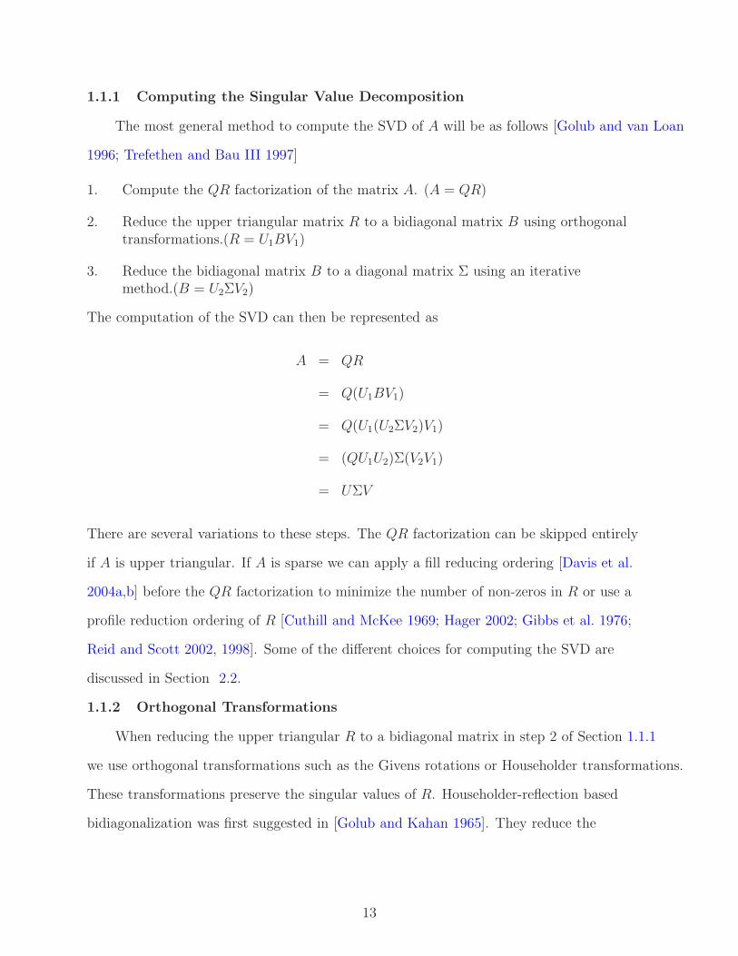
1.1.1 Computing the Singular Value Decomposition
The most general method to compute the SVD of A will be as follows [Golub and van Loan
1996; Trefethen and Bau III 1997]
1. Compute the QR factorization of the matrix A. (A = QR)
2. Reduce the upper triangular matrix R to a bidiagonal matrix B using orthogonaltransformations.(R = U1BV1)
3. Reduce the bidiagonal matrix B to a diagonal matrix Σ using an iterativemethod.(B = U2ΣV2)
The computation of the SVD can then be represented as
A = QR
= Q(U1BV1)
= Q(U1(U2ΣV2)V1)
= (QU1U2)Σ(V2V1)
= UΣV
There are several variations to these steps. The QR factorization can be skipped entirely
if A is upper triangular. If A is sparse we can apply a fill reducing ordering [Davis et al.
2004a,b] before the QR factorization to minimize the number of non-zeros in R or use a
profile reduction ordering of R [Cuthill and McKee 1969; Hager 2002; Gibbs et al. 1976;
Reid and Scott 2002, 1998]. Some of the different choices for computing the SVD are
discussed in Section 2.2.
1.1.2 Orthogonal Transformations
When reducing the upper triangular R to a bidiagonal matrix in step 2 of Section 1.1.1
we use orthogonal transformations such as the Givens rotations or Householder transformations.
These transformations preserve the singular values of R. Householder-reflection based
bidiagonalization was first suggested in [Golub and Kahan 1965]. They reduce the
13
sub-diagonal part of an entire column in a dense matrix to zero with one Householder
transformation.
In the case of band matrices both Givens rotations [Schwarz 1968; Rutishauser 1963;
Kaufman 2000] and Householder transformations [Bischof et al. 2000b; Murata and Horikoshi
1975] have been used in the past to reduce it to a bidiagonal matrix. While Householder
transformations operate on entire columns at a time we would like to zero entries
selectively in a sparse or band bidiagonalization step, so we will use Givens rotations
in both the cases.
1.2 Singular Value Decomposition of Sparse and Band Matrices
The SVD of sparse and band matrices poses various challenges. Some of these
problems are also faced by many other numerical algorithms and some problems are
unique to this problem. We discuss these issues here.
Data structure. We assume that the band matrices are stored in a packed column
band format i.e if A ∈ Rm×n and the lower bandwidth is l and the upper bandwidth is
u then we store A in a (l + u + 1) × n matrix B such that A(i, j) = B(i − j + u + 1, j)
[Golub and van Loan 1996]. Besides the advantage of reduced space, this column based
data structure, enables the use of column based algorithms which can then be adapted
to the sparse bidiagonal reduction. Sparse matrices are usually stored in a compressed
column format with only the non-zeroes stored. However, we need more space than that
for sparse bidiagonal reduction algorithm. We present two profile data structures for the
storing a sparse matrix in order to compute the SVD efficiently.
Fill-in. Almost all sparse matrix algorithms have some ways to handle fill-in: trying
to reduce the fill-in by reordering the matrix or doing a symbolic factorization to find
the exact fill-in etc. The former ensures that the amount of work and memory usage is
reduced. The later ensures a static data structure which leads to predictable memory
accesses in turn improving the performance. We apply our Givens rotations in a pipelined
scheme and avoid any fill-in in the band reduction algorithms. See Chapter 3 for more
14
details. We cannot avoid the fill-in in the sparse case, but we try to minimize the fill-in by
choosing to reduce the columns that generate the least amount of fill first. See Chapter 5
for more details. It is better to avoid the Householder transformations in the sparse case
because of the catastrophic fill they might generate.
FLOPS. Floating point operations or FLOPS measures the amount of work
performed by a numerical algorithm. Generally, an increase in the fill-in leads to more
floating point operations. Our band reduction algorithms do no more work than a simple
non-blocked band reduction algorithm due to fill. However, they do more floating point
operations than the non-blocked algorithms due to the order in we choose to do the
reduction. The increase in the floating point operations is due to blocking, but the
advantage of blocking overwhelms the small increase in FLOPS. We also show how to
accumulate the left and right singular vectors by operating on just the non-zeroes thereby
reducing the number of floating point operations required.
The sparse case, uses a dynamic blocking scheme for finding a block of plane rotations
that can be applied together. The algorithm for sparse bidiagonal reduction tries to do
the least amount of work, but there is no guarantee for doing the least amount of FLOPS
for sparse matrices. However, given a band matrix the sparse algorithm will do the same
amount of FLOPS as the blocked band reduction algorithm.
Memory access. Performance of any algorithm gets impacted by the number
of times they access the memory and the order in which they access the memory.
The development of the Basic Linear Algebra Subroutines (BLAS) [Blackford et al.
2002; Dongarra et al. 1990] and algorithms that use the BLAS mainly focus on this
aspect. Unfortunately, generating Givens rotations and applying them are BLAS-1 style
operations leading to poor performance. Blocked algorithms tend to work around this
problem. We present blocked algorithms for both the sparse and band bidiagonalization
cases. The symbolic factorization algorithm for bidiagonal reduction of sparse matrices
helps us allocate a static data structure for the numerical reduction step.
15
Software. Availability of usable software for these linear algebraic algorithms play
a crucial role in getting the algorithms adapted. We have developed software for band
reduction and for computing the SVD of a sparse matrix.
In short, we have developed algorithms for blocked bidiagonal reduction of band
matrices and sparse matrices that take into consideration memory usage, operation count,
caching, symbolic factorization and data structure issues. We also present robust software
implementing these algorithms.
Modified versions of Chapters 3 and 5, which discuss blocked algorithms for band
reduction and sparse SVD respectively, will be submitted to ACM Transactions on
Mathematical Software as two theory papers [Rajamanickam and Davis 2009a]. The
software for band reduction (discussed in Chapter 4 and in [Rajamanickam and Davis
2009b]) and the software for sparse bidiagonal reduction will be submitted to ACM
Transactions on Mathematical Software as Collected Algorithms of the ACM.
16
CHAPTER 2LITERATURE REVIEW
We summarize past research related to singular value decomposition, band reduction,
sparse singular value decomposition in this chapter. The problem of band reduction,
especially with respect to the symmetric reduction to tridiagonal matrix case, has been
studied for nearly 40 years. Section 2.1 presents the past work in band reduction. The
singular value decomposition problem for dense matrices has been studied for several
years and various iterative methods are known for finding the sparse singular value
decomposition too. These are described in Section 2.2.
2.1 Givens Rotations and Band Reduction
Givens rotations (or plane rotations as it is called now) and Jacobi rotations [Schwarz
1968; Rutishauser 1963] are used in the symmetric eigenvalue problem of band matrices,
especially to reduce the matrix to the bidiagonal form. The Givens rotations themselves,
in their present unitary form, are defined in [Givens 1958]. It takes a square root and
5 floating point operations (flops) to compute the Givens rotations and two values to
save them. Stewart [1976] showed how we can save just one value, the angle of the
rotation, and save some space. The computation of the square root is one of the expensive
operations in modern computers. Square root free Givens rotations are discussed in
[Hammarling 1974; Gentleman 1973; Anda and Park 1994]. Bindel et al. [2002] showed
that it was possible to accurately find the Givens rotation without overflow or underflow.
Rutishauser [1963] gave the first algorithm for band reduction using a pentadiagonal
matrix. This algorithm removes the fill caused by a plane rotation [Givens 1958]
immediately with another rotation. Schwarz generalized this method for tridiagonalizing
a symmetric band matrix [Schwarz 1963, 1968]. Both algorithms use plane rotations (or
Jacobi rotations) to zero one non-zero entry of the band resulting in a scalar fill. The
algorithms then use new plane rotations to reduce the fill, creating new fill further down
17
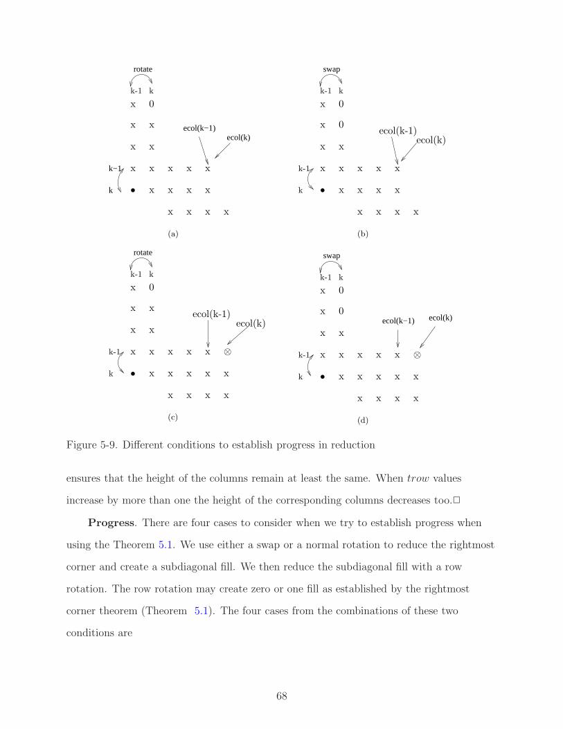
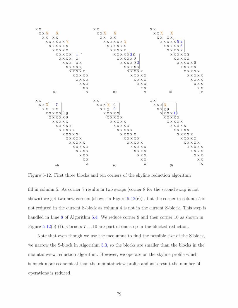
(c)
x x x x xx xx
x x x x x xx x
x x x x x xx x
x x x x x xx x •
x x x x 1x
x x x x x x x
x x x x x xx x•
x x x xx xxx
x x x x x x
x x x x x
x x x x
x x x
x x x x x xx x
x x x x x xx
x x x x xx xx
x x x x x xx x
x x x x x xx x
x x x x x xx x
x x 4 2 03
x x x x x x x
x x x x x xx x
x x x xx xxx
x x x x x x
x x x x x
x x x x
x x x
x x x x x xx x
x x x x x xx
x x x x xx 3x
x x x x x xx 4
x x x x x xx x
x x x x x xx x
x x x x 0x
x x x x x x 2
x x x x x xx x
x x x xx xxx
x x x x x x
x x x x x
x x x x
x x x
x x x x x xx x
x x x x x xx
(a) (b)
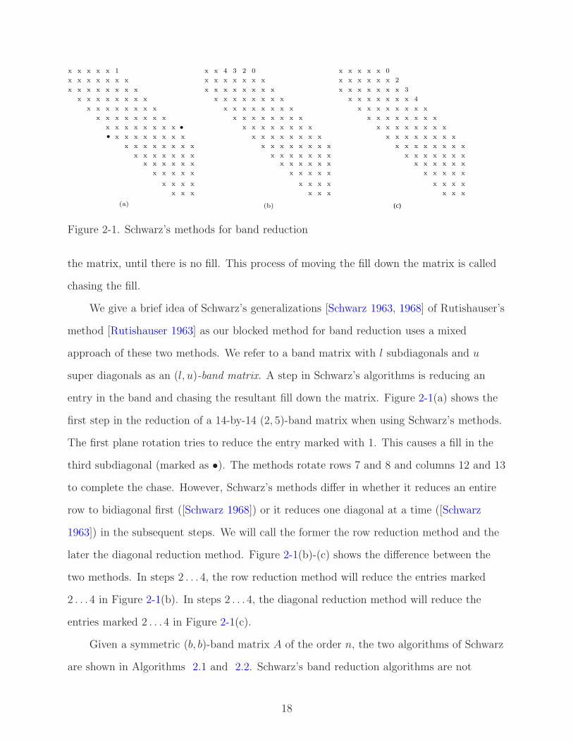
Figure 2-1. Schwarz’s methods for band reduction
the matrix, until there is no fill. This process of moving the fill down the matrix is called
chasing the fill.
We give a brief idea of Schwarz’s generalizations [Schwarz 1963, 1968] of Rutishauser’s
method [Rutishauser 1963] as our blocked method for band reduction uses a mixed
approach of these two methods. We refer to a band matrix with l subdiagonals and u
super diagonals as an (l, u)-band matrix. A step in Schwarz’s algorithms is reducing an
entry in the band and chasing the resultant fill down the matrix. Figure 2-1(a) shows the
first step in the reduction of a 14-by-14 (2, 5)-band matrix when using Schwarz’s methods.
The first plane rotation tries to reduce the entry marked with 1. This causes a fill in the
third subdiagonal (marked as •). The methods rotate rows 7 and 8 and columns 12 and 13
to complete the chase. However, Schwarz’s methods differ in whether it reduces an entire
row to bidiagonal first ([Schwarz 1968]) or it reduces one diagonal at a time ([Schwarz
1963]) in the subsequent steps. We will call the former the row reduction method and the
later the diagonal reduction method. Figure 2-1(b)-(c) shows the difference between the
two methods. In steps 2 . . . 4, the row reduction method will reduce the entries marked
2 . . . 4 in Figure 2-1(b). In steps 2 . . . 4, the diagonal reduction method will reduce the
entries marked 2 . . . 4 in Figure 2-1(c).
Given a symmetric (b, b)-band matrix A of the order n, the two algorithms of Schwarz
are shown in Algorithms 2.1 and 2.2. Schwarz’s band reduction algorithms are not
18
blocked algorithms. Rutishauser [1963] modified the Givens method [Givens 1958] for
reducing a full symmetric matrix to tridiagonal form to use blocking. The structure of
the block, a parallelogram, will be the same for the modified Givens method and our
algorithm, but we will allow the number of columns and number of rows in the block to
be different. Furthermore, [Rutishauser 1963] led to a bulge-like fill which is expensive to
chase, whereas our method results in less intermediate fill which takes much less work to
chase.
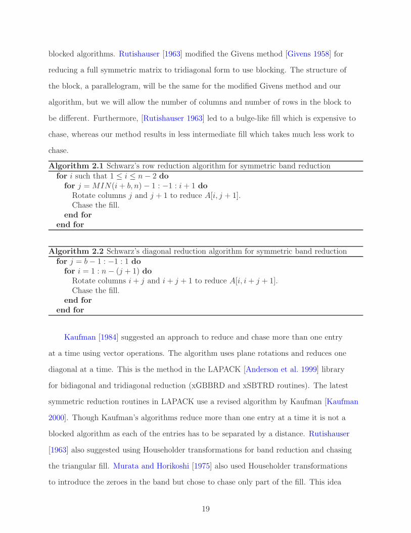
Algorithm 2.1 Schwarz’s row reduction algorithm for symmetric band reduction
for i such that 1 ≤ i ≤ n − 2 dofor j = MIN(i + b, n) − 1 : −1 : i + 1 do
Rotate columns j and j + 1 to reduce A[i, j + 1].Chase the fill.
end forend for
Algorithm 2.2 Schwarz’s diagonal reduction algorithm for symmetric band reduction
for j = b − 1 : −1 : 1 dofor i = 1 : n − (j + 1) do
Rotate columns i + j and i + j + 1 to reduce A[i, i + j + 1].Chase the fill.
end forend for
Kaufman [1984] suggested an approach to reduce and chase more than one entry
at a time using vector operations. The algorithm uses plane rotations and reduces one
diagonal at a time. This is the method in the LAPACK [Anderson et al. 1999] library
for bidiagonal and tridiagonal reduction (xGBBRD and xSBTRD routines). The latest
symmetric reduction routines in LAPACK use a revised algorithm by Kaufman [Kaufman
2000]. Though Kaufman’s algorithms reduce more than one entry at a time it is not a
blocked algorithm as each of the entries has to be separated by a distance. Rutishauser
[1963] also suggested using Householder transformations for band reduction and chasing
the triangular fill. Murata and Horikoshi [1975] also used Householder transformations
to introduce the zeroes in the band but chose to chase only part of the fill. This idea
19
reduced the flops required, but increased the workspace. Recently, Lang [1993] used this
idea for parallel band reduction. The idea is also used in the SBR tool box [Bischof et al.
2000b]. However, they use QR factorization of the subdiagonals and store it as WY
transformations [Van Loan and Bischof 1987] so that they can take advantage of level
3 style BLAS operations. The SBR framework can choose to optimize for floating point
operations, available work space and using the BLAS.
In order to compute the singular vectors we can start with an identity matrix
and apply the plane rotations to it. There are two types of methods to do this: we
apply the plane rotations when they are applied to the original band matrix (forward
accumulation) or we save all the rotations and apply it to the identity matrices later
(backward accumulation)[Smith et al. 1976]. Even though simple forward accumulation
requires more floating point operations than backward accumulation, Kaufman [1984]
showed that we can do forward accumulation efficiently by exploiting the non zero pattern
when applying the rotations to the identity. Kaufman’s accumulation algorithm will do
the same number of floating point operations as backward accumulation. The non zero
pattern of U or V will be dependent upon the order in which we reduce the entries in the
original band matrix. The accumulation algorithm exploits the non zero pattern of U or V
while using our blocked reduction.
2.2 Methods to Compute the Singular Value Decomposition
Golub and Kahan [1965] introduced the two step approach to compute the singular
value decomposition. In order to compute the SVD of A they reduce A to a bidiagonal
matrix and then reduce the bidiagonal matrix to a diagonal matrix (the singular values).
Golub and Reinsch [1970] introduced the QR algorithm to compute the second step.
Demmel and Kahan [1990] showed that the singular values of the bidiagonal matrix can be
computed accurately. The two step method was modified to a three step method described
in Section 1.1.1 by Chan [Chan 1982]. The bidiagonalization was preceded by a QR
factorization step followed by the bidiagonalization of R. This method leads to less work
20
whenever m ≥ 5n/3. [Trefethen and Bau III 1997] suggest a dynamic approach where one
starts with bidiagonalization first and switches to QR factorization when appropriate. We
will use the three step approach for computing the SVD.
Sparse SVD. Iterative methods like the Lanczos or subspace iteration based
algorithms in SVDPACK [Berry 1992] and PROPACK [Larsen 1998] are available for
finding the sparse SVD. The main advantage of these iterative methods is their speed
when only a few singular values are required. However, we have to guess the required
number of singular values when we use the iterative algorithms. There is no known direct
method to compute all the singular values of a sparse matrix.
Other methods and applications. The Singular value decomposition is one of
the factorizations that has its uses in a diverse group of applications. Latent Semantic
Indexing based applications use the SVD of large sparse matrices [Berry et al. 1994;
Deerwester et al. 1990]. The SVD is also used in collaborative filtering [Pryor 1998;
Paterek 2007; Goldberg et al. 2001; Billsus and Pazzani 1998] and recommender systems
[Sarwar et al. 2002; Koren 2008]. Sparse graph mining applications that need to find
patterns can do so efficiently with the SVD. Compact Matrix Decomposition (CMD)
[Sun et al. 2008] or the approximate versions [Drineas et al. 2004] do better than SVD
now. Other applications include gene expression analysis [Wall et al. 2003], finding the
pseudo inverse of a matrix [Golub and Kahan 1965] and solving the linear least squares
problem [Golub and Reinsch 1970]. There are other alternative methods to compute
the bidiagonal reduction. One sided bidiagonal reductions are discussed in [Ralha 2003;
Barlow et al. 2005; Bosner and Barlow 2007] and the semidiscrete decomposition (SDD)
[Kolda and O’leary 1998] was proposed as an alternative to SVD itself.
21
CHAPTER 3BAND BIDIAGONALIZATION USING GIVENS ROTATIONS
3.1 Overview
Eigenvalue computations of symmetric band matrices depend on a reduction to
tridiagonal form [Golub and van Loan 1996]. Given a symmetric band matrix A of size
n-by-n with l subdiagonals and super diagonals, the tridiagonal reduction can be written
as
UT AU = T (3–1)
where T is a tridiagonal matrix and U is orthogonal. Singular value decomposition of an
m-by-n unsymmetric band matrix A with l subdiagonals and u super diagonals depends
on a reduction to bidiagonal form. We can write the bidiagonal reduction of A as
UT AV = B (3–2)
where B is a bidiagonal matrix and U and V are orthogonal.
Some of the limitations of existing band reduction methods [Bischof et al. 2000a;
Kaufman 1984] can be summarized as follows:
• they lead to poor cache access and they use expensive non-stride-one access rowoperations during the chase (or)
• they use more memory and/or more work to take advantage of cache friendly BLAS3style algorithms.
In this chapter, we describe an algorithm that uses plane rotations, blocks the
rotations for efficient use of cache, does not generate more fill than non blocking
algorithms, performs only slightly more work than the scalar versions, and avoids
non-stride-one access as much as possible when applying the blocked rotations.
Section 3.2 introduces the blocking idea. Blocking combined with pipelined rotations
helps us achieve minimal fill, as discussed in Section 3.3. We introduce the method to
accumulate the plane rotations efficiently in Section 3.4. The performance results for the
new algorithms are in Section 3.5.
22
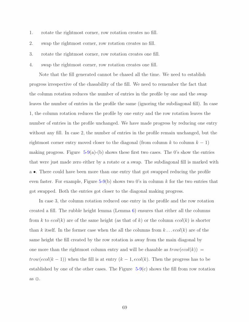
D block
S block
C block
R block
F block
(c)
x x x x xx xx
x x x x x xx x
x x x x x xx x
x x x x x xx x
x x x ⊗ ⊗⊗
x x x x ⊗ ⊗ ⊗
x x x x x xx x
x x x xx xxx
x x x x x x
x x x x x
x x x x
x x x
x x x x x xx x
x x x x x xx
x x x x xx xx
x x x x x xx x
x x x ⊗ ⊗⊗
x x x x ⊗ ⊗ ⊗
x x x xx x• xx
x x x x x x
x x x x x
x x x x x xx
x x x x x •x• x x
x x x x •xxx x
• x x x x
• x x x
x x x x x x •• xx
x x x x x x• x x •
x x x x ⊗⊗ ⊗x
x x x x ⊗ ⊗x ⊗
x x x x x xx x
x x x x x xx x
x x x 0 00
x x x x 0 0 0
x x x x x xx x
x x x xx xxx
x x x x x x
x x x x x
x x x x
x x x
x x x x x xx x
x x x x x xx
(a) (b)
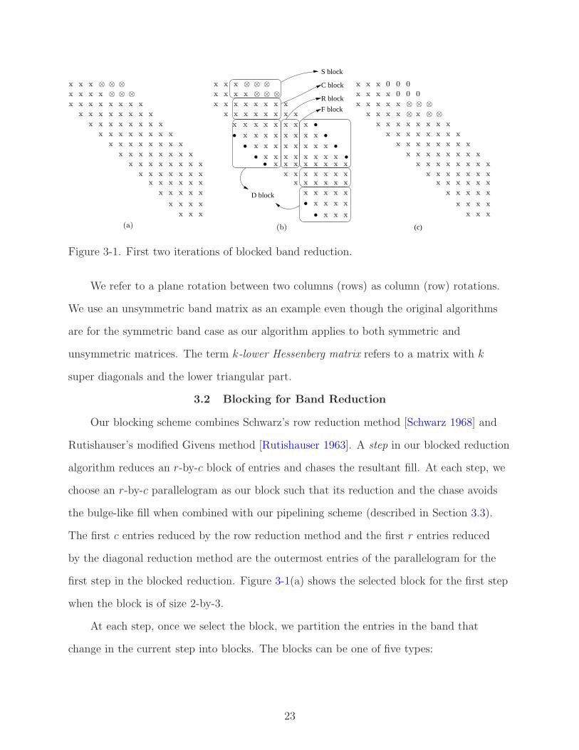
Figure 3-1. First two iterations of blocked band reduction.
We refer to a plane rotation between two columns (rows) as column (row) rotations.
We use an unsymmetric band matrix as an example even though the original algorithms
are for the symmetric band case as our algorithm applies to both symmetric and
unsymmetric matrices. The term k-lower Hessenberg matrix refers to a matrix with k
Rutishauser’s modified Givens method [Rutishauser 1963]. A step in our blocked reduction
algorithm reduces an r-by-c block of entries and chases the resultant fill. At each step, we
choose an r-by-c parallelogram as our block such that its reduction and the chase avoids
the bulge-like fill when combined with our pipelining scheme (described in Section 3.3).
The first c entries reduced by the row reduction method and the first r entries reduced
by the diagonal reduction method are the outermost entries of the parallelogram for the
first step in the blocked reduction. Figure 3-1(a) shows the selected block for the first step
when the block is of size 2-by-3.
At each step, once we select the block, we partition the entries in the band that
change in the current step into blocks. The blocks can be one of five types:
23
S-block The S (seed) block consists of the r-by-c parallelogram to be reduced and the
entries in the same r rows as the parallelogram to which the rotations are applied.
The S-block in the upper (lower) triangular part is reduced with column (row)
rotations.
C-block The C (column rotation) block has the entries that are modified only by column
rotations in the current step.
D-block The D (diagonal) block consists of the entries that are modified by both column
and row rotations (in that order) in the current step. Applying column rotations
in this block causes fill which are chased by new row rotations. This is at most a
(c + r)-by-(c + r) block.
R-block The R (row rotation) block has the entries that are modified only by row
rotations in the current step.
F-block The F (fill) block consists of the entries that are modified by both row and
column rotations (in that order) in the current step. Applying row rotations in
this block causes fill which is chased by new column rotations. This is at most a
(c + r)-by-(c + r) block.
Generally the partitioning results in one seed block and potentially more than one
of the other blocks. The blocks other than the seed block repeat in the same order. The
order of the blocks is C, D, R and F-block when the seed block is in the upper triangular
part. Figure 3-1(b) shows all the different blocks for the first step. The figure shows more
than one fill, but no more than one fill is present at the same time. The fill is limited to
a single scalar. The pipelining (explained in Section 3.3) helps us restrict the fill. As a
result, our method uses very little workspace other than the matrix being reduced and an
r-by-c data structure to hold the coefficients for the pending rotations being applied in a
single sweep.
Once we complete the chase in all the blocks, subsequent steps reduce the next r-by-c
entries in the same set of r rows as long as there are more than r diagonals left in them.
24
This results in the two pass algorithm where we reduce the bandwidth to r first and then
reduce the thin band to a bidiagonal matrix. Figure 3-1(c) highlights the entries for the
second step with ⊗. The two pass band reduction is given in Algorithm 3.1. The while
loop in Line 1 reduces the bandwidth to r and is taken at most twice.
Algorithm 3.1 Two pass algorithm for band reduction
1: while lowerbandwidth > 0 or upperbandwidth > 1 do2: for each set of r rows/columns do3: reduce the band in lower triangular part4: reduce the band in upper triangular part5: end for6: set c to r − 17: set r to 1.8: end while
There are two exceptions with respect to the the number of diagonals left. The
number of diagonals left in the lower triangular part is r − 1 instead of r, when r is one (to
avoid the second iteration of the while loop in the above algorithm) and when the input
matrix is an unsymmetric (l, 1)-band matrix (for more predictable accumulation of the
plane rotations). See Section 3.4 for more details on the later.
The algorithm so far assumes the number of rows in the block for the upper
triangular part and the number of columns in the block for the lower triangular part
are the same. We reduce the upper and lower triangular part separately if that is not
the case. Algorithm 3.2 reduces the band in the upper triangular part. The algorithm
for reducing the lower triangular part is similar to the one for the upper triangular part
except that the order of the blocks in the chasing is different. In the inner while loop the
rotations are applied to the R, F, C and D-blocks, in that order.
3.3 Pipelining the Givens Rotations
The algorithm for the reduction of the upper triangular part in Section 3.2 relies
on finding and applying the plane rotations on the blocks. Our pipelining scheme does
not cause triangular fill-in and avoids non-stride-one access of the matrix. The general
idea is to find and store r-by-c rotations in the workspace and apply them as efficiently
25
Algorithm 3.2 Algorithm for band reduction in the upper triangular part
1: for each set of c columns in current set of rows do2: Find the trapezoidal set of entries to zero in this iteration3: Divide the matrix into blocks4: Find column rotations to zero r-by-c entries in the S-block and apply them in the
S-block5: while column rotations do6: Apply column rotations to the C-block7: Apply column rotations to the D-block, Find row rotations to chase fill8: Apply row rotations to the R-block9: Apply row rotations to the F-block, Find column rotations to chase fill
10: Readjust the four blocks to continue the chase.11: end while12: end for
as possible in each of the blocks to extract maximum performance. Figures 3-2 - 3-6
in this section show the first five blocks from Figure 3-1(b) and the operations in all of
them are sequentially numbered from 1..96. A solid arc between two entries represents
the generation of a row (or column) rotation between adjacent rows (or columns) of the
matrix to annihilate one of the two entries in all the figures in this section. A dotted arc
represents the application of these rotations to other pairs of entries in the same pair of
rows (or columns) of the matrix.
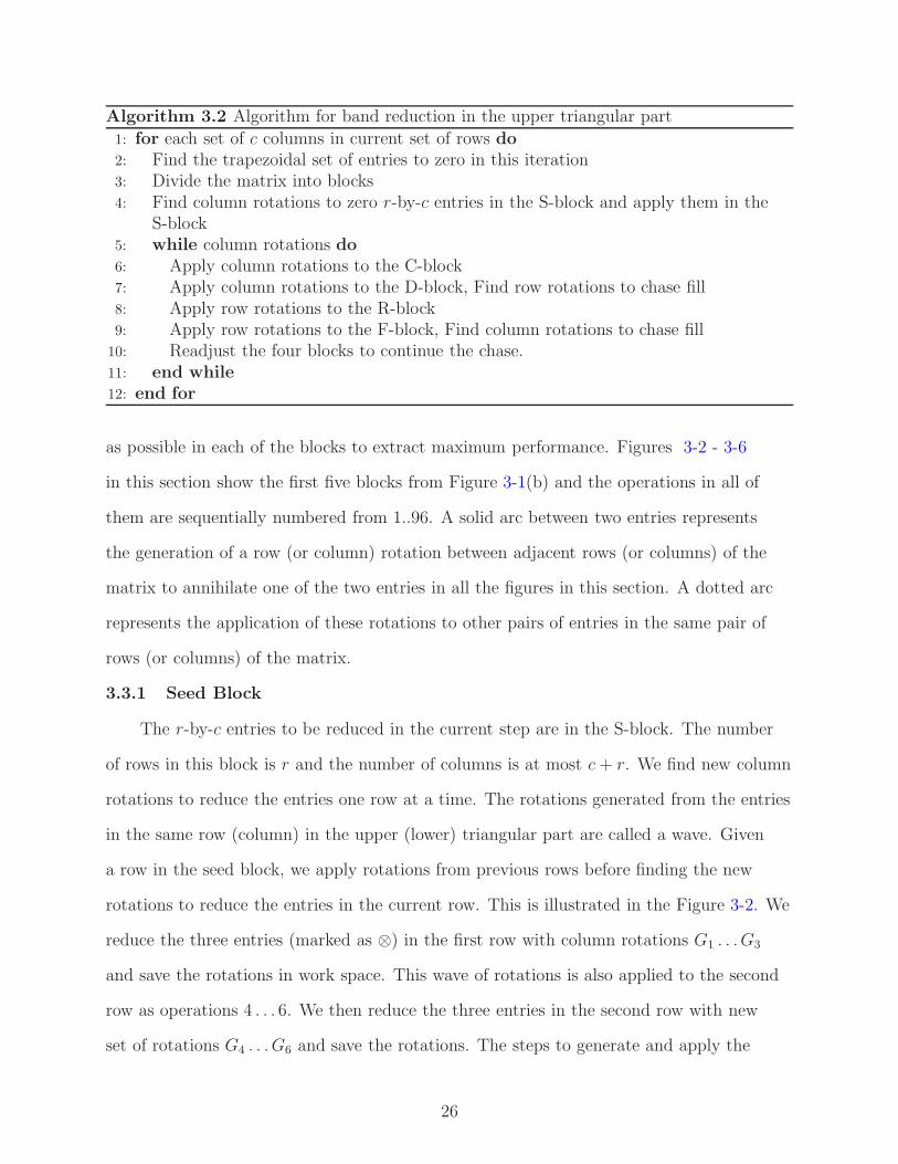
3.3.1 Seed Block
The r-by-c entries to be reduced in the current step are in the S-block. The number
of rows in this block is r and the number of columns is at most c + r. We find new column
rotations to reduce the entries one row at a time. The rotations generated from the entries
in the same row (column) in the upper (lower) triangular part are called a wave. Given
a row in the seed block, we apply rotations from previous rows before finding the new
rotations to reduce the entries in the current row. This is illustrated in the Figure 3-2. We
reduce the three entries (marked as ⊗) in the first row with column rotations G1 . . . G3
and save the rotations in work space. This wave of rotations is also applied to the second
row as operations 4 . . . 6. We then reduce the three entries in the second row with new
set of rotations G4 . . . G6 and save the rotations. The steps to generate and apply the
26
0 0 0x456
x x x x x
G3 G2 G1
0 0 0x
x x ⊗⊗⊗
G4G5G6
x ⊗⊗⊗
x x x xx
G3 G2 G1
(b) (c)(a)
Figure 3-2. Finding and applying column rotations in the S-block
(a) (b)
G4G5G6
x xxx x
161820
x xxx x171921
x xxx x
x xxx x
101214
111315
G1G2G3
Figure 3-3. Applying column rotations to the C-block.
rotations in the S-block are shown in Algorithm 3.3. Finding and applying rotations in the
S-block is the only place in the algorithm where we use explicit non-stride-one access to
access the entries across the rows.
Algorithm 3.3 Generating and applying rotations in the S-block
1: for all rows in the S-block do2: if not the first row then3: apply column rotations from the previous rows.4: end if5: Find the column rotations to zero entries in current row (if there are any)6: end for
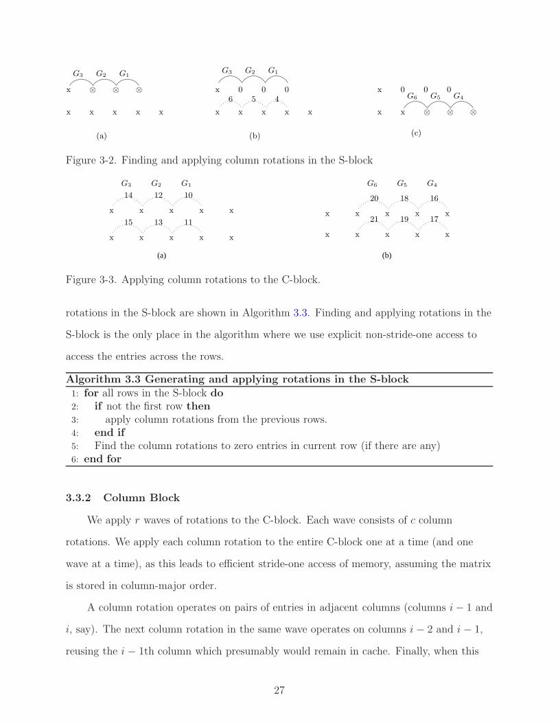
3.3.2 Column Block
We apply r waves of rotations to the C-block. Each wave consists of c column
rotations. We apply each column rotation to the entire C-block one at a time (and one
wave at a time), as this leads to efficient stride-one access of memory, assuming the matrix
is stored in column-major order.
A column rotation operates on pairs of entries in adjacent columns (columns i − 1 and
i, say). The next column rotation in the same wave operates on columns i − 2 and i − 1,
reusing the i − 1th column which presumably would remain in cache. Finally, when this
27
RG1
RG2
RG3
G1G2G3
22
23
24
2526
27
28
2930
31
3233
• x x x
x x xxx
x x xx•
x x•
x
RG2
RG3
RG1
x x xxx
x x xx
x x x
x x
x
36
37
38
39 42
40
4135
34
RG4
RG5
RG6
G4G5G6
x x xxx
• x
• x x
• x x x
x x xx
48
53
45
46
47
50
51
52
55
56
434954
44
57
RG5
RG6
RG4
x x xxx
x x xx
x x x
x x
x
62
6360
59
61
58
(b)
(a)
Figure 3-4. Applying column rotations and finding row rotations in the D-block.
first wave is done we repeat and apply all the remaining r − 1 waves to the corresponding
columns of the C-block. The column rotations in any wave j + 1 use all but one column
used by the wave j leading to possible cache reuse. Figure 3-3(a)-(b) illustrates the order
in which we apply the two waves of rotations (G1 . . . G3 and G4 . . . G6) to the 2 rows in the
C-block. Algorithm 3.4 describes these steps to apply the rotations in the C-block.
Algorithm 3.4 Applying rotations in the C-block
1: for each wave of column rotations do2: for each column in this wave of rotations do3: Apply the rotation for the current column from current wave to all the rows in the
C-block.4: end for5: Shift column indices for next wave.6: end for
28
x
x
x
66
65
64
x
RG3
RG2
RG1
RG4
RG5
RG6
x x
x
x
x
x
69
68
67
Figure 3-5. Applying row rotations to one column in the R-block.
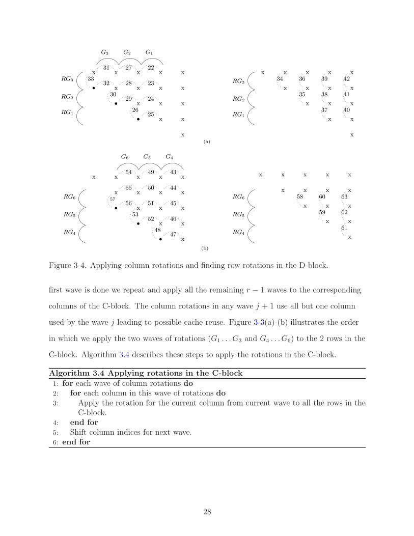
3.3.3 Diagonal Block
We apply r waves each with c column rotations to the D-block. Each column rotation
Gi (say between columns k and k − 1) can generate a fill in this block. In order to restrict
the fill to a scalar, we reduce the fill immediately with a row rotation (RGi) before we
apply the next column rotation Gi+1 (to columns k − 1 and k − 2). We save the row
rotation after reducing the fill and continue with the next column rotation Gi+1, instead
of applying the row rotation to the rest of the row as that would lead to non-stride-one
access. When all the column rotations in the current wave are done, we apply the new
wave of row rotations to each column in the D-block.
This algorithm leads to two sweeps on the entries of the D-block for each wave of
column rotations: one from right to left when we apply column rotations that generate
fill, find row rotations, reduce the fill and save the row rotations, and the next from left
to right when we apply the pipelined row rotations to all the columns in the D-block.
We repeat the two sweeps for each of the subsequent r − 1 waves of column rotations.
Figure 3-4(a) shows the order in which we apply the column rotations G1 . . . G3, find the
corresponding row rotations and apply them to our example. The operations 22 . . . 42
show these steps. Operations 22 . . . 33 show the right to left sweep and 34 . . . 42 show
the left to right sweep. Figure 3-4(b) shows the order in which we apply a second wave
of rotations G4 . . .G6 to our example and handle the fill generated by them (numbered
43 . . . 63). Algorithm 3.5 shows both applying and finding rotations in the D-block.
29
Algorithm 3.5 Applying and finding rotations in the D-block
1: for each wave of column rotations do2: for each column in this wave of rotations (right-left) do3: Apply the rotation for the current column from current wave to all the
rows in the D-block, generate fill.4: Find row rotation to remove fill.5: Apply row rotation to remove fill. (not to entire row)6: end for7: for each column in this wave of rotations (left-right) and additional columns in the
D-block to the right of these columns do8: Apply all pending row rotations to current column.9: end for
10: Shift column indices for next wave.11: end for
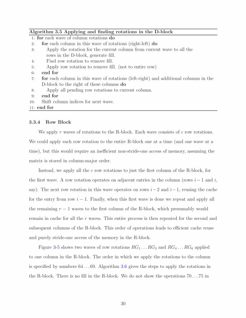
3.3.4 Row Block
We apply r waves of rotations to the R-block. Each wave consists of c row rotations.
We could apply each row rotation to the entire R-block one at a time (and one wave at a
time), but this would require an inefficient non-stride-one access of memory, assuming the
matrix is stored in column-major order.
Instead, we apply all the c row rotations to just the first column of the R-block, for
the first wave. A row rotation operates on adjacent entries in the column (rows i− 1 and i,
say). The next row rotation in this wave operates on rows i−2 and i−1, reusing the cache
for the entry from row i − 1. Finally, when this first wave is done we repeat and apply all
the remaining r − 1 waves to the first column of the R-block, which presumably would
remain in cache for all the r waves. This entire process is then repeated for the second and
subsequent columns of the R-block. This order of operations leads to efficient cache reuse
and purely stride-one access of the memory in the R-block.
Figure 3-5 shows two waves of row rotations RG1 . . . RG3 and RG4 . . . RG6 applied
to one column in the R-block. The order in which we apply the rotations to the column
is specified by numbers 64 . . . 69. Algorithm 3.6 gives the steps to apply the rotations in
the R-block. There is no fill in the R-block. We do not show the operations 70 . . . 75 in
30
RG3
RG1
RG2
x x x xx
xxx
xx
x xxx
x
76
77
78
79
80
81
x x x xx
x xxx
•xxx
•xx
•x
90
89
88
87
92
93
94
95
96
83
84
85
82
86
91
G1G2G3
RG3
RG1
RG2
Figure 3-6. Applying row rotations and finding column rotations in the F-block
the second column of the R-block (from Figure 3-1(b)) in the Figure 3-5. But the row
rotations are applied in the same pattern as in the first column.
Algorithm 3.6 Applying rotations in the R-block
1: for each column in the R-block do2: for each wave of row rotations do3: Apply all the rotations in current wave to appropriate rows in current column.4: Shift row indices for next wave.5: end for6: end for
3.3.5 Fill Block
We apply r waves each with c row rotations to the F-block. Each row rotation RGp
(between rows i and i − 1 say) can create a fill in this block. We could adopt the same
approach as in the D-block, completing the row rotation RGp in this block to generate the
fill and using a column rotation to reduce the fill immediately before we do row rotation
RGp+1, to restrict the fill to a scalar, but that would require us to access all the entries in
a row.
Instead, for each column in the F-block we apply all the relevant row rotations from
the current wave, but just stop short of creating any fill. Note that we need not apply all
c row rotations to all the columns of the F-block. When applying the row rotations to a
column, successive row rotations share entries between them for maximum cache reuse as
in the R-block. This constitutes one left-to-right sweep of all the entries in the F-block.
31
We then access the columns from right to left by applying the row rotation say RGp
(between rows i and i − 1 say) that generates the fill in that column of the F-block (say
k), remove the fill immediately with column rotation Gp and apply the column rotation to
rest of the entries in columns k and k − 1 in the F-block.
Figure 3-6 shows the order in which we apply the row rotations (operations 76 . . . 81),
generate fill (operations 82, 86, 91), and apply the column rotations. Operations 76 . . . 81
constitute the left-to-right sweep. Operations 82 . . . 96 constitute the right-to-left sweep.
We repeat this for all the r − 1 pending waves of rotations. Algorithm 3.7 shows the two
phases in applying the rotations in the F-block.
Algorithm 3.7 Applying row rotations and finding column rotations in the F-block
1: for each wave of row rotations do2: for each column in the F-block (left-right) do3: Apply all rotations from current wave, except those that generate fill-in in the
current column, to current column.4: end for5: for each column in the F-block (right-left) do6: Apply the pending rotation that creates fill.7: Find column rotation to remove fill.8: Apply column rotation to entire column.9: end for
10: Shift row indices for next wave.11: end for
To summarize, the only non-stride-one access we do in the entire algorithm is in the
seed block when we try to find the rotations. We generate no more fill than the any of
the scalar algorithms by pipelining our plane rotations. The amount of work we do varies
based on the block size which is explained in the next subsection.
3.3.6 Floating Point Operations for Band Reduction
For the purposes of computing the exact number of floating point operations, we
assume that finding a plane rotation takes six operations, as in the real case with no
scaling of the input parameters (two multiplications, two divides, one addition and a
32
square root). We also assume that applying the plane rotations to two entries requires six
floating point operations as in the real case (four multiplications and two additions).
Let us consider the case of reducing a (u, u)-symmetric band matrix of order n to
tridiagonal form by operating only on the upper triangular part of the symmetric matrix.
The number of floating point operations required to reduce the symmetric matrix using
Schwarz’s diagonal reduction method is
fd = 6
b∑
d=3
n∑
i=d
d + 2
⌊
max (i − d, 0)
d − 1
⌋
(d + 1) + rem
(
max (i − d, 0)
d − 1
)
+ 2 (3–3)
where rem is the remainder function and b = u + 1. The number of floating point
operations required to reduce the symmetric matrix using Schwarz’s row reduction method
is
fr = 6n−2∑
i=1
min(b,n−i+1)∑
d=3
d + 2
⌊
max (i − d, 0)
b − 1
⌋
(b + 1) + rem
(
max (i − d, 0)
b − 1
)
+ 2 (3–4)
In order to find the number of of floating point operations for our blocked reduction,
when block size is r-by-c we note that we perform the same number of operations as
using a two step Schwarz’s row reduction method where we first reduce the matrix to r
diagonals using Schwarz’s row reduction method and then reduce the r diagonals using
Schwarz’s row reduction again. Then we can obtain the floating point operations required
by the blocked reduction to reduce the matrix by using the equation 3–4 for fr.
fb1 =
n−r−1∑
i=1
min(b,n−i+1)∑
d=r+2
d + 2
⌊
max (i − d, 0)
b − 1
⌋
(b + 1) + rem
(
max (i − d, 0)
b − 1
)
+ 2 (3–5)
fb2 =n−2∑
i=1
min(r+1,n−i+1)∑
d=3
d + 2
⌊
max (i − d, 0)
r
⌋
(r + 2) + rem
(
max (i − d, 0)
r
)
+ 2 (3–6)
fb = 6 (fb1 + fb2) (3–7)
33
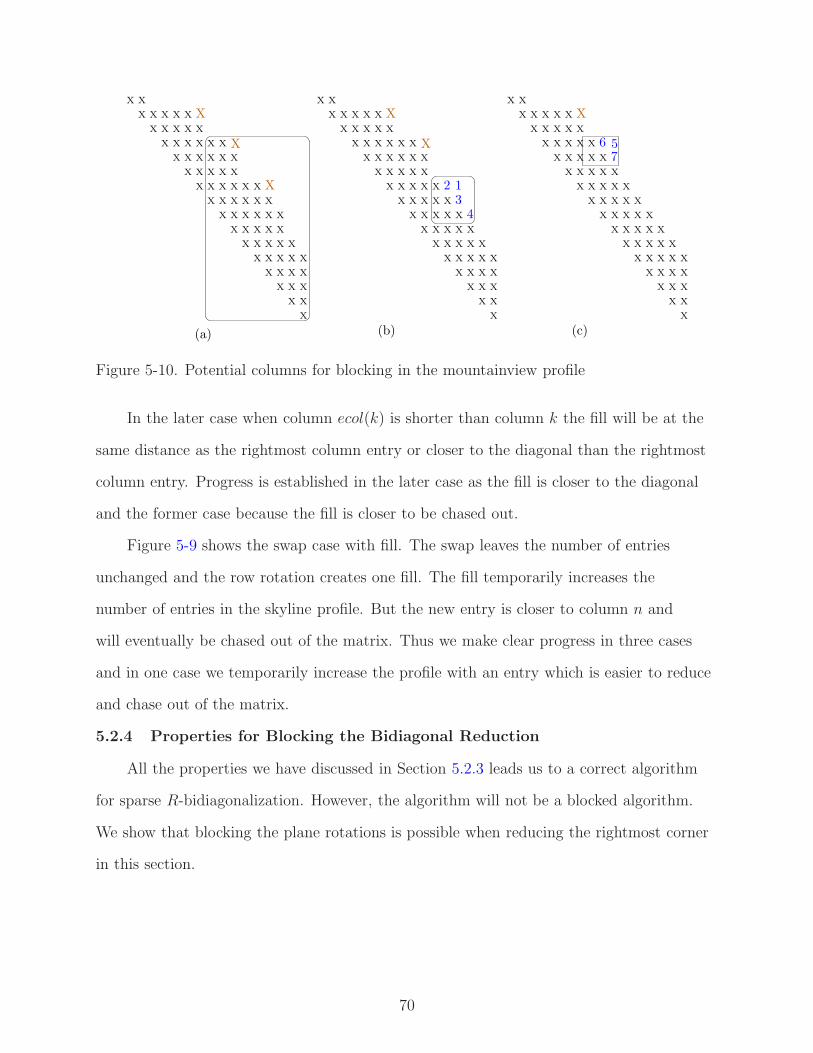
X X ⊕ ⊕ ⊕ ⊕ ⊕
X X X X X X X
X X X X X X X
X X X X X X X
X X X X X X X
X X X X X
X X X X X X X
X X X X X X X
X X X X X X X
X X X X X X X
X X X X X X
X X X X
X X X
X X
X
X 5 3 2 1X 4 X
X X X X
X X X X X X
X X
X X X
X X X X X
X X X X X X
X X
X X X
X X X
5 4 3 2 1 X
5 4 3 2 X 1
5 4 3 X 2
5 4 X 3
5 X 4
X 5
X
X X X X X X •
◦ ◦ ◦ ◦ ◦ X X ◦
• • • • • X X X X X X ◦
• • • • • X X ◦
• • • • • X X X ◦
• • • • • X X X X ◦
• • • • X X X X X ◦•
• • • • • X X X X X X ◦
X X X X X •
X X X X •
X X X •
X X •
X X X X X X •
◦ ◦ ◦ ◦ ◦ X X X
◦ ◦ ◦ ◦ ◦ X X X
(a) (b) (c)
Figure 3-7. Update of U for symmetric A with r = 1
Asymptotically, all three methods result in the same amount of work. But the work
differs by a constant factor. All three methods require the same amount of work when
u < 3. Given a 1000-by-1000 matrix and u = 3, Schwarz’s row reduction method can
compute the bidiagonal reduction with 10% fewer floating point operations (flops) than
the diagonal reduction method. Depending on the block size, the blocked method does
the same number of floating point operations as one of the other two methods. When
we increase the bandwidth to u = 150 for the same matrix, the row reduction method
results in 10% fewer flops than the diagonal reduction method and 3% fewer flops than
the blocked reduction method (with default block size). When the input matrix is dense
(u = 999), the row reduction method performs 25% fewer flops than the diagonal
reduction method and 5% fewer flops than the blocked method (with default block size).
The row reduction method in this example leads to the least flops, but the blocked
reduction is only 3-5% worse in terms of the flops. We show that this can be compensated
by the performance advantage of blocking.
3.4 Accumulating the Plane Rotations
Our blocked approach to the band reduction leads to a different non-zero pattern
in U and V than the one described by Kaufman [2000]. In this section, we describe the
34
X X X X 3 2 1
X X X X 6 5 4
X X X X X X X
X X X X X
X X X X ⊕ ⊕ ⊕
X X X X X X X
X X X X X X X
X X X X X X X
X X X X X X
X X X X
X X X
X
X
X X X X 9 8 7
X X X ⊕ ⊕ ⊕
X X X X ⊕ ⊕ ⊕
X
X
X
X
X
X X X X
X X X X X X
X X X X X
X X X X X X
X X X X X
X X X X
X
9 8 7 X
3 2 1 X 4 7
3 2 X 1 4 7
3 X 2 5 8
X 3 6 9
6 5 4 X 7
X
X
X
• • • X X X X ◦ ◦ ◦
• • • X X X X X ◦ ◦
• • • X X X X X X ◦
• • • X X X X X ◦
• • • X X X X ◦
• • • X X X X X X ◦
◦ ◦ ◦ X
X X X X • • •
X X X X X • • •
X X X X X X • • •
X X X X X X • • •
X X X X X • • •
X X X X • • •
Figure 3-8. Update of U for symmetric A with r = 3
fill pattern in U and V for our blocked reduction method. The accumulation algorithm
uses the fact that applying plane rotations between any two columns in U results in the
non-zero pattern of both the columns to be equal to the union of the original non-zero
pattern of the columns. Given an identity matrix U to start with and the order of the
plane rotations, as dictated by the blocked reduction, we need to track the first and last
non zero entries in any column of U to apply the rotations only to the non-zeros. It is easy
to do this for U and V if we have two arrays of size n, but we use constant space to do the
same. In this section, we ignore the numerical values and use only the symbolic structure
of U . We omit V from the discussion hereafter as the fill pattern in V will be the same as
the fill pattern in U .
3.4.1 Structure of U
A step in our blocked reduction Algorithm 3.1 reduces a block of entries. We define
a major step as the reduction from one iteration of the for loop in Line 2 of Algorithm
3.1. A minor step is defined as the reduction in one iteration of the while loop in line 5 of
Algorithm 3.2. In other words, a major step can involve many steps to reduce one set of r
columns and/or rows to a bandwidth of r. A step can involve many minor steps to chase
the fill to the end of the matrix.
35
3 X X X X X X X X
X X X X X X X X X X X
X X X X X X X X X
X X X X X X X X X X X
X X X X X X X X X X X
X X X X X X X X X X X
X X X X X X X X X X X
X X X X X X X X X X
X X X X X X X X
X X X X X X X
X X X X X X
X X X X X
1 X X X X X X X X X X
2 X X X X X X X X X
4 X X X X X X X
X e d c b aX X 4
4 3 X 2
4 3 2 X 1
4 3 2 1 X
X
X X X
X
X
X
X
X X
X X X X
X X X X X
X X X X X X
X
4 X 3
X X
X X X
X X X X
X X X X X
X X X X X
• • • • X •
• • • • • X X X
X •
• X •
• • X •
• • • • • X X
• • • • • X X X X
• • • • • X X X X X
• • • • • X X X X X X
X
• • • X •
(a) (b) (c)
Figure 3-9. Update of U for unsymmetric A with r = 1
Given a band matrix A and a r-by-c block, the algorithm to find the non zero pattern
in U differs based on four possible cases
• A is a symmetric or A is an unsymmetric (0, u)-band matrix.
• A is an unsymmetric (l, 1)-band matrix.
• A is an unsymmetric (l, u)-band matrix where l > 0, u > 1 and r = 1.
• A is an unsymmetric (l, u)-band matrix where l > 0, u > 1 and r > 1.
The structure of the algorithm is the same in all four cases. Applying the plane
rotations from the first major step, i.e, reduction of the first r columns and/or rows of
A, to the identity matrix U leads to a specific non zero pattern in the upper and lower
triangular part of U . This non zero pattern in U then dictates the pattern of the fill in U
while applying the plane rotations from the subsequent major steps.
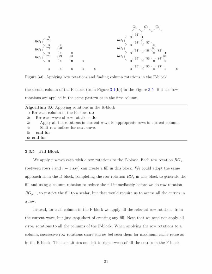
Symmetric A: We consider a symmetric (u, u)-band matrix and an unsymmetric
(0, u)-band matrix as symbolically equivalent in this section as we operate only on the
upper triangular part of the symmetric matrix. When A is a symmetric (u, u)-band
matrix and r = 1, our reduction Algorithm 3.1 reduces each row to bidiagonal form
before reducing any entries in the subsequent rows. When reducing the first row of A to
bidiagonal form, the u − 1 plane rotations from the first minor step applied to columns
36
2 . . . u + 1 of U , results in a block fill in U where the block is a lower Hessenberg matrix
of the the order u. The fill in U , from the next u − 1 plane rotations (from the next
minor step of the chase in A), is in the subsequent u columns of U and has the same lower
Hessenberg structure. When we apply all the plane rotations from the first major step
in the reduction of A we get a block diagonal U , where each block is lower Hessenberg
of order u. For example, consider reducing the first row of entries marked 1 . . . 5 in the
Figure 3-7(a). Figure 3-7(b) shows the fill pattern after applying to U the plane rotations
that were generated to reduce these entries and chase the resultant fill. The fill in U ,
generated from the first minor step of the reduction of A is marked with the corresponding
number of the entry from Figure 3-7(a) that caused the fill. For example, fill from entry
marked 3 in Figure 3-7(a) is marked 3 in Figure 3-7(b). The fill in U from the subsequent
minor steps are marked x.
Applying the plane rotations from reducing every other row of A (and the corresponding
chase) results in a u-by-(u − 1) block fill for each minor step in the lower triangular part
of U (until it is full) and an increase in one super diagonal. Figure 3-7(c) shows the fill in
U caused by the plane rotations from the second major step. The fill from the first minor
step is marked with • and the fill from subsequent minor steps are marked with ◦. Note
that keeping track of the fill in the upper triangular part is relatively easy as all plane
rotations that reduce entries from row k and the corresponding chase generate fill in the
k-th super diagonal of U . This fill pattern in U is exactly same as the fill pattern in U if
we reduced A with Schwarz’s row reduction method (Algorithm 2.1), as blocked reduction
follows the same order of rotations when r is one.
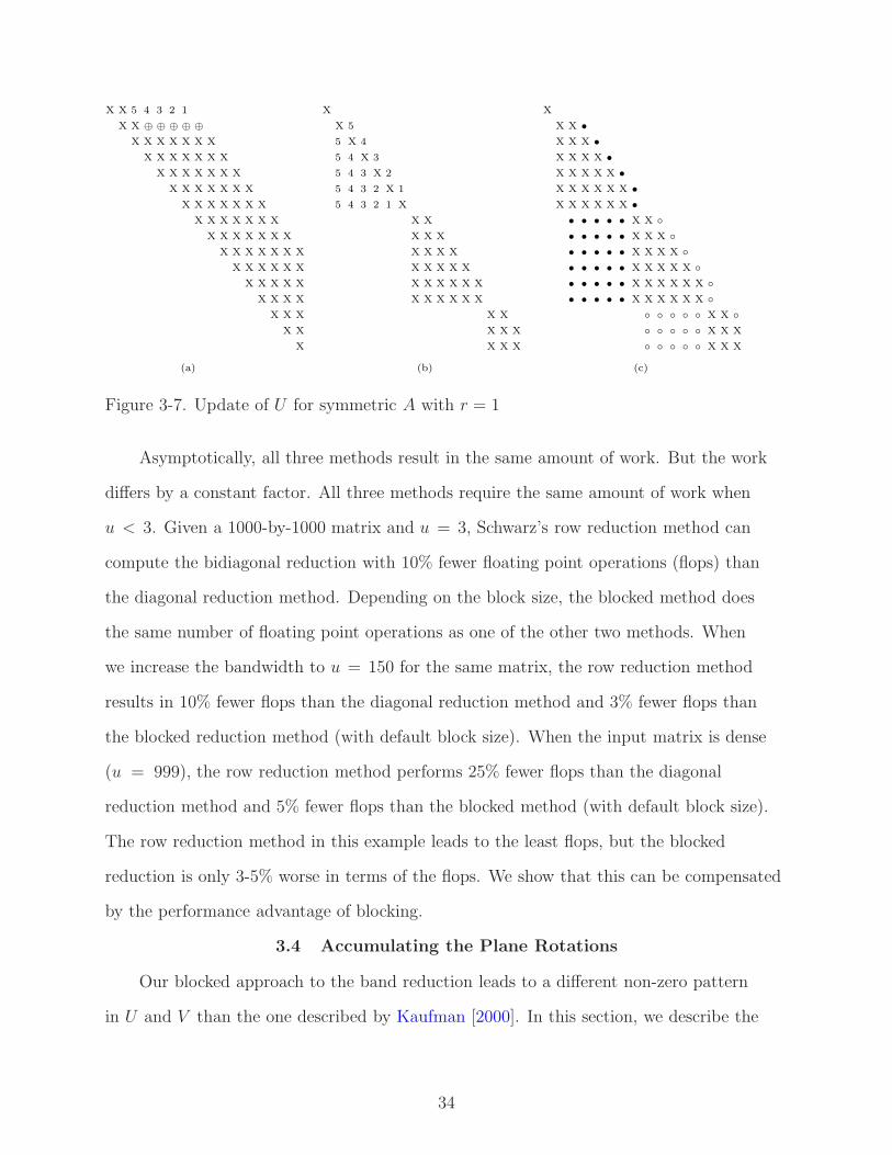
When r > 1 each block in the block diagonal U , after applying the rotations from the
first major step to U , is a (u − r, r)-band matrix of the order u. Each subsequent minor
step generates a block fill in U that consists of a (u − r + 1)-by-(u − r) block and below
that a block of (0, u − r)-band matrix with a zero diagonal. The example given below
illustrates this case clearly. As discussed in the r = 1 case, there is also an addition of r
37
super diagonals in U , for every r rows that are reduced in A. Figure 3-8 shows the fill in U
for the first two major steps when r = 3. The conventions are same as before. In the first
major step (Figure 3-8(b))the fill from first minor step is numbered for the entries in A
(Figure 3-8(a)) that caused the fill, and further fill from the other minor steps are shown
as x. In the second major step (Figure 3-8(c)), the fill from two different minor steps are
differentiated with • and ◦. Furthermore, the two blocks of fill in the lower triangular part
of U for one minor step are bounded with rectangles in Figure 3-8(c).
(l, 1)-band A: Given a (l, 1)-band matrix the band reduction algorithm reduces
the lower triangular part to r − 1 diagonals to keep the pattern of the fill in U simple.
When r = 1, applying the rotations from the first major step of the reduction leads
to a block diagonal U , with each block lower Hessenberg of the order l + 1. Applying
rotations from each subsequent major step, results in rectangular blocks of fill of the order
of (l + 1)-by-l in the lower triangular part of U , and one additional super diagonal in the
upper triangular part of U . The basic structure of the fill is similar to the one shown in
Figure 3-7(b)-(c) except the size of the blocks is different.
When r > 1, applying rotations from the first major step results in a block diagonal
U , where each block is (l− r +2, r)-band of the order (l +1). Applying rotations from each
subsequent major step results in a block of fill that consists of a (l − r + 2)-by-(l − r + 1)
block and below that a block in the shape of (0, l − r + 1)-band of the order (r − 1)-by-l
with a zero diagonal in the lower triangular part of U , and r additional super diagonals in
the upper triangular part of U . The basic structure of the fill is similar to the one shown
in Figure 3-8(b)-(c) except the size of the blocks is different.
Unsymmetric A, r = 1: When we consider the case of the unsymmetric (l, u)-band
matrix A, to find the non zero pattern of U , we need to only look at the interaction
between the plane rotations to reduce the entries in lower triangular part and the plane
rotations to chase the fill from lower triangular part (even though the original entries were
from the upper triangular part), as these are the only rotations applied to U . We can
38
X X X X X X X X X
2 X X X X X X X X X
1 4 X X X X X X X X X
X X X X X X X X X X X
X X X X X X X X X
3 X X X X X X X X X X
X X X X X X X X X X X
X X X X X X X X X X X
X X X X X X X X X X X
X X X X X X X X X X
X X X X X X X X
X X X X X X X
X X X X X X
X X X X X
X X X d c b a
X X X X h g f e
X
X
X 2 4
2 X 1 3
2 1 X 3
X
X
4 3 X
X
X
X
X
X X X
X X X X
X X X X
X X X
X
X
X X X
X X X X
X X X X
X X X
X X X
X X X X
X X X X
X X X
h g f e X
d c b a X e
d c b X a e
d c X b f
d X c g
X d h
X X X X 0 0 0 0
X X X X X ⊕ ⊕ ⊕ ⊕
X X X X X X X X X X X
X X X X X X X X X
⊗ ⊗ X X X X X X X X X
⊗ X X X X X X X X X X
X X X X X X X X X X X
X X X X X X X X X X
X X X X X X X X
X X X X X X X
X X X X X X
X X X X X
0 0 X X X X X X X X X
0 X X X X X ⊕ ⊕ ⊕ ⊕
X X X 0 0 0 0
0 ⊗ X X X X X X X X X
X
X
X X X X
X X X X
X X X X
X X X
• • X X X
• • X X X X
• • X X X X X
• • X X X X X X
• • X X X X X X
• • X X X X X
X X X • •
X X X X • •
X X X X • •
X X X • •
X
X
X X X X X
X X X X X X
X X X X X X
X X X X X X X • •
X X X X X
X X X X X X • •
X X X X X X X • •
• • • • X X X X
• • • • X X X X
• • • • X X X X
• • • • X X X
X X X X X X X X • •
X X X X X X X X • •
X X X X X • •
(a) (b) (c)
(f)(e)(d)
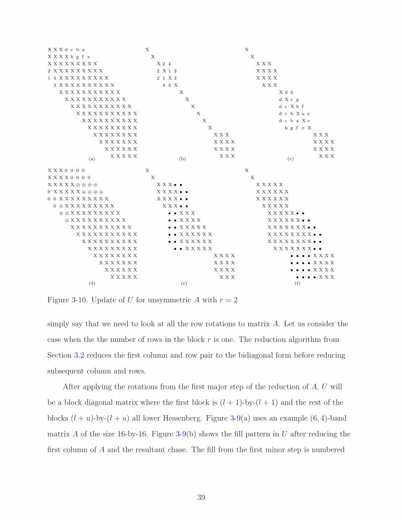
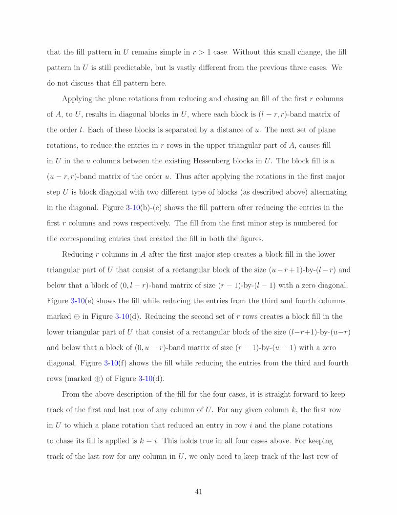
Figure 3-10. Update of U for unsymmetric A with r = 2
simply say that we need to look at all the row rotations to matrix A. Let us consider the
case when the the number of rows in the block r is one. The reduction algorithm from
Section 3.2 reduces the first column and row pair to the bidiagonal form before reducing
subsequent column and rows.
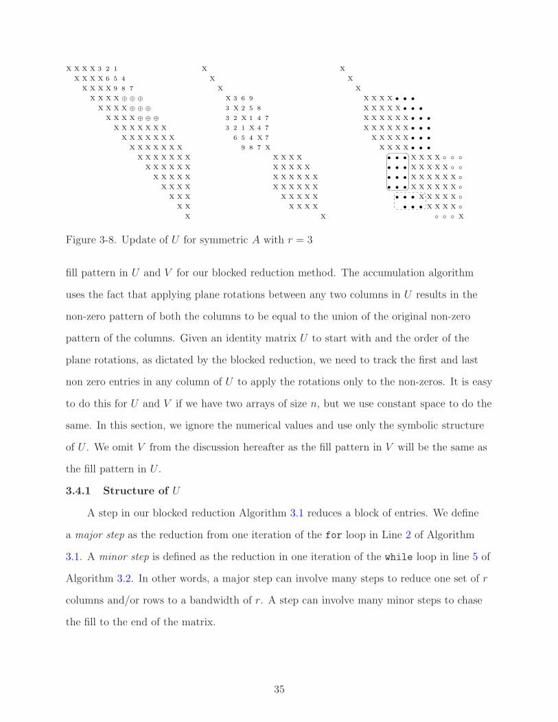
After applying the rotations from the first major step of the reduction of A, U will
be a block diagonal matrix where the first block is (l + 1)-by-(l + 1) and the rest of the
blocks (l + u)-by-(l + u) all lower Hessenberg. Figure 3-9(a) uses an example (6, 4)-band
matrix A of the size 16-by-16. Figure 3-9(b) shows the fill pattern in U after reducing the
first column of A and the resultant chase. The fill from the first minor step is numbered
39
for the corresponding entries that caused it. Figure 3-9(c) shows the fill pattern in U after
the first major step . All the new fill is marked with •.
Each subsequent minor step results in a block fill of size (l + u)-by-(l + u − 1) in U in
the lower triangular part, except the first block which is of size (l + u)-by-l. The fill in the
upper triangular part of U is still one super diagonal for a every column and row pair. The
structure of the fill in U is similar to Figure 3-7(c) except the size of the blocks is larger.
The reason for the block Hessenberg structure when applying the plane rotations
in the first major step is not straight forward as in the symmetric case, but we describe
it here for completeness. The plane rotations to reduce the entries in the first column is
between rows l + 1 . . . 1 resulting in a lower Hessenberg block of the size (l + 1)-by-(l + 1)
in U as we saw in the symmetric case. The plane rotations from the corresponding chase
results in the same lower Hessenberg block structure fill in U , but each of these blocks
is separated by u − 1 columns (not u). When we reduce the first row later, the plane
rotations are between columns (u + 1) . . . 2 of A. Note that column u + 1 of A should have
been involved in the chase to reduce the fill generated from reducing the entry A(1, 2) (as
l > 0). When we reduce the entry in A(1, u + 1) and chase the resultant subdiagonal fill,
applying the plane rotation to U results in fill of size l + 2 in the lower triangular part of
U . This fill is caused by the existing Hessenberg blocks in U of order l + 1. In other words,
as column u + 1 in A is part of the chase when reducing the first column of A and part of
the actual reduction when reducing the entries in first row of A the interaction of the fill
leads to a bigger Hessenberg block of order (l + u).
Unsymmetric A, r > 1: When r > 1 the reduction Algorithm 3.1 leaves r diagonals
in the upper and lower triangular part, whereas when r = 1 above we reduce the matrix
to bidiagonal in one iteration, which is equivalent to leaving r − 1 diagonals in the lower
triangular part. We need to leave r diagonals in the lower triangular part instead of r − 1
diagonals consistent with the r = 1 case to avoid the one column interaction between the
plane rotations of the lower and upper triangular part as explained above in r = 1 case, so
40
that the fill pattern in U remains simple in r > 1 case. Without this small change, the fill
pattern in U is still predictable, but is vastly different from the previous three cases. We
do not discuss that fill pattern here.
Applying the plane rotations from reducing and chasing an fill of the first r columns
of A, to U , results in diagonal blocks in U , where each block is (l − r, r)-band matrix of
the order l. Each of these blocks is separated by a distance of u. The next set of plane
rotations, to reduce the entries in r rows in the upper triangular part of A, causes fill
in U in the u columns between the existing Hessenberg blocks in U . The block fill is a
(u − r, r)-band matrix of the order u. Thus after applying the rotations in the first major
step U is block diagonal with two different type of blocks (as described above) alternating
in the diagonal. Figure 3-10(b)-(c) shows the fill pattern after reducing the entries in the
first r columns and rows respectively. The fill from the first minor step is numbered for
the corresponding entries that created the fill in both the figures.
Reducing r columns in A after the first major step creates a block fill in the lower
triangular part of U that consist of a rectangular block of the size (u− r +1)-by-(l− r) and
below that a block of (0, l − r)-band matrix of size (r − 1)-by-(l − 1) with a zero diagonal.
Figure 3-10(e) shows the fill while reducing the entries from the third and fourth columns
marked ⊕ in Figure 3-10(d). Reducing the second set of r rows creates a block fill in the
lower triangular part of U that consist of a rectangular block of the size (l−r+1)-by-(u−r)
and below that a block of (0, u − r)-band matrix of size (r − 1)-by-(u − 1) with a zero
diagonal. Figure 3-10(f) shows the fill while reducing the entries from the third and fourth
rows (marked ⊕) of Figure 3-10(d).
From the above description of the fill for the four cases, it is straight forward to keep
track of the first and last row of any column of U . For any given column k, the first row
in U to which a plane rotation that reduced an entry in row i and the plane rotations
to chase its fill is applied is k − i. This holds true in all four cases above. For keeping
track of the last row for any column in U , we only need to keep track of the last row of
41
the first block of U and V and update it after each major step based on the above four
cases. While reducing a particular set of r column and rows and chasing the fill we can
obtain the last row for a given column from the last row of the first block and the number
of minor steps completed and the fill size based on the above cases. We leave the indexing
calculations out of the chapter for a simpler presentation.
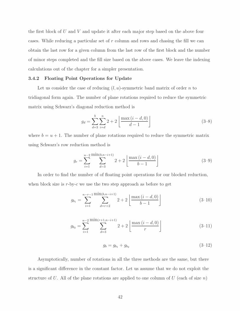
3.4.2 Floating Point Operations for Update
Let us consider the case of reducing (l, u)-symmetric band matrix of order n to
tridiagonal form again. The number of plane rotations required to reduce the symmetric
matrix using Schwarz’s diagonal reduction method is
gd =
b∑
d=3
n∑
i=d
2 + 2
⌊
max (i − d, 0)
d − 1
⌋
(3–8)
where b = u + 1. The number of plane rotations required to reduce the symmetric matrix
using Schwarz’s row reduction method is
gr =n−2∑
i=1
min(b,n−i+1)∑
d=3
2 + 2
⌊
max (i − d, 0)
b − 1
⌋
(3–9)
In order to find the number of of floating point operations for our blocked reduction,
when block size is r-by-c we use the two step approach as before to get
gb1 =n−r−1∑
i=1
min(b,n−i+1)∑
d=r+2
2 + 2
⌊
max (i − d, 0)
b − 1
⌋
(3–10)
gb2 =
n−2∑
i=1
min(r+1,n−i+1)∑
d=3
2 + 2
⌊
max (i − d, 0)
r
⌋
(3–11)
gb = gb1 + gb2 (3–12)
Asymptotically, number of rotations in all the three methods are the same, but there
is a significant difference in the constant factor. Let us assume that we do not exploit the
structure of U . All of the plane rotations are applied to one column of U (each of size n)
42
then. Reducing the number of plane rotations plays a significant role in reducing the flops
for accumulation of the plane rotations.
Given a 1000-by-1000 matrix, and l = 150, Schwarz’s row reduction method computes
the bidiagonal reduction using 78% fewer plane rotations than the diagonal reduction
method. It performs 43% fewer plane rotations than the blocked reduction method (with
the default block size). When l = 999, the the row reduction method computes 83% and
48% fewer plane rotations than the diagonal reduction and blocked reduction methods
respectively. The increase in the number of plane rotations for the blocked method is due
to the rotations to reduce the r diagonals as a second iteration (gb2 in Equation 3–11).
These rotations are especially costly they are applied to a full U .
We can exactly mimic the Schwarz’s row reduction and still do blocking by choosing
r = 1, leading to a 50% reduction in the flop count. Note that the cost of small increase
in the flops when we reduce A without the accumulation was offset by the blocking, but
in this case, when the flops almost doubles it is important to use r = 1. The default
block size will use r = 1 when the plane rotations are accumulated. Unless there are some
compelling reasons, say improvements like blocking the accumulation in U itself which
offsets the cost in flops r > 1 case will be practically slower when U and V are required.
3.5 Performance Results
We compare our band reduction routine piro band reduce against that of SBR’s
driver routine DGBRDD [Bischof et al. 2000a] and LAPACK’s symmetric and unsymmetric
routines DSBTRD and DGBBRD [Anderson et al. 1999] in this section. All the tests were
done with double precision arithmetic with real matrices. The performance measurements
were done on a machine with 8 dual core 2.2 GHz AMD Opteron processors, with 64GB
of main memory. PIRO BAND was compiled with gcc 4.1.1 with the options -O3.
LAPACK and SBR are compiled with g77 with the options -O3 -funroll-all-loops.
Figure 3-11 shows the raw performance of our algorithms with the default block
size used by our routines. We estimate the default block size based on the problem size.
43
107
108
109
1010
1011
1012
5
6
7
8
9
10
11
x 108 PIRO_BAND : Performance
FLOPS
FLO
PS
/sec
bw=150
bw=200
bw=300
bw=400
bw=500
Figure 3-11. Performance of the blocked reduction algorithm with default block sizes
107
108
109
1010
1011
0.8
1
1.5
2
3
4PIRO_BAND vs SBR performance
FLOPS
SB
R ti
me/
PIR
O_B
AN
D ti
me
bw=150bw=200bw=300bw=400bw=500
107
108
109
1010
1011
0.8
1
1.5
2
3
4PIRO_BAND vs LAPACK performance
FLOPS
LAP
AC
K ti
me/
PIR
O_B
AN
D ti
me
bw=150bw=200bw=300bw=400bw=500
Figure 3-12. Performance of piro band reduce vs SBR and LAPACK
44
0 2000 4000 6000 8000 100000.5
0.8
1
1.5
2
3PIRO_BAND vs LAPACK performance w/ update
NLA
PA
CK
tim
e/P
IRO
_BA
ND
tim
e
bw=150bw=200bw=300bw=400bw=500
0 1000 2000 3000 4000 5000 60000.5
0.8
1
1.5
2
3PIRO_BAND vs SBR performance w/ update
N
SB
R ti
me/
PIR
O_B
AN
D ti
me
bw=150bw=200bw=300bw=400bw=500
Figure 3-13. Performance of piro band reduce vs SBR and LAPACK with update
108
109
1010
1011
1
2
3
4
5
6
7
8
9PIRO_BAND vs DGBBRD performance
FLOPS
DG
BB
RD
tim
e/P
IRO
_BA
ND
tim
e
bw=150bw=200bw=300bw=400bw=500
0 500 1000 1500 2000 2500 30001
2
3
4
5
6
7
8
9PIRO_BAND vs DGBBRD performance w/ update
N
DG
BB
RD
tim
e/P
IRO
_BA
ND
tim
e
bw=150bw=200bw=300bw=400bw=500
Figure 3-14. Performance of piro band reduce vs DGBBRD of LAPACK
45
The block size estimate is not based on hardware or compiler parameters. Performance
of our algorithms depend to some extent on the block size. The optimal block sizes
can vary depending on the architecture, compiler optimizations and problem size. The
default block size is not the optimal block size for all the problems, even in this particular
machine. Nevertheless, the results from default block size is used for all the performance
comparisons in this section. The effects of the different block sizes on the performance are
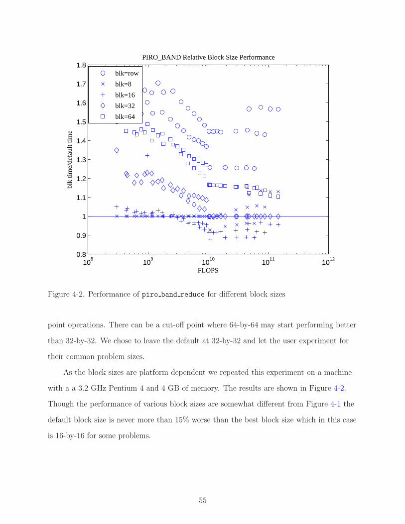
discussed in [Rajamanickam and Davis 2009b] and in Section 4.3.1
Figure 3-11 shows the effect of blocking for different bandwidths. The tests were
run on symmetric matrices of the order 200 to 10000 with bandwidths 150 to 500.
The band reduction algorithm performs slightly better for problems with non-narrow
bandwidths than for the problems with narrow bandwidths. The figure shows the effect
of cache: helping the performance for smaller matrices and then negatively affecting the
performance as the problem size increases, but blocking stabilizes the performance as the
problem size increases.
Given a problem size, we use the floating point operations from the Schwarz’s row
reduction method as the flops required for that problem. The different algorithms we
compare may do more floating point operations than Schwarz’s row reduction method (no
algorithm will do less). We use the smallest possible flops for a given problem (the flops
from Schwarz’s row reduction method) as a baseline to compare all the algorithms. The
graphs in Figures 3-11, 3-12, 3-14 use the FLOPS from Schwarz’s row reduction method.
Figure 3-12 compares the performance of our blocked algorithm and SBR’s band
reduction routines, without the accumulation of plane rotations. We provide SBR the
maximum workspace it requires n × u for a matrix of size (u, u)-band matrix of order n
and let it choose the best possible algorithm. For smaller matrices, SBR is about 20%
faster than our algorithm. When the problems get larger, for smaller bandwidths, the
performance of both the algorithms are comparable even though the work space required
by our algorithm is considerably smaller (32-by-32). As the bandwidth increases our
46
blocked algorithm is about 25% to 2x faster than SBR algorithms while using only fraction
of the work space.
The results of the performance comparison against LAPACK’s DSBTRD is shown in
Figure 3-12. LAPACK’s routines does not have any tuning parameters except the size n
workspace required by the routines. DSBTRD performs slightly better than our algorithm
for smaller problem sizes. As the problem sizes increase, our algorithm is faster than
DSBTRD even for smaller bandwidths. The performance improvement is in the order of 1.5x
to 3.5x. DSBTRD uses the revised algorithm as described in [Kaufman 1984].
When we accumulate the plane rotations we use one entire row of the symmetric
matrix as our block as this cuts the floating point operations required by nearly half when
compared to a block size of 32-by-32. The performance of our algorithm against SBR and
LAPACK algorithms are shown in the Figure 3-13. Our algorithm is faster than SBR
by a factor 2.5 for larger matrices. It is 20% to 2 times faster than LAPACK’s DSBTRD
implementation. As in the no accumulation case, the larger the bandwidth the better the
performance improvement for our algorithm.
We compare our algorithm against LAPACK’s DGBBRD for the unsymmetric case.
DGBBRD does not use the revised algorithm of Kaufman yet, so it can do better in the
update case. The results when we compare our algorithm against the existing version of
DGBBRD are in Figures 3-14 without and with the accumulation of plane rotations. Our
algorithm is about 4 to 7 times faster in the former case and about 2 to 8 times faster in
the later case.
3.6 Summary
The problem of band reduction had two possible style of solutions: a vectorized
solution using plane rotations implemented in LAPACK libraries and a BLAS3 based
solution using QR factorization and Householder transformations implemented in
SBR toolbox. We presented a blocked algorithm in this chapter that is better than
the competitive methods in terms of the required workspace, the number of floating point
47
operations and real performance. The software package that implements this algorithm,
PIRO BAND, is described in detail in Chapter 4.
48
CHAPTER 4PIRO BAND: PIPELINED PLANE ROTATIONS FOR BAND REDUCTION
4.1 Overview
Band reduction methods are an important part of algorithms for eigen value
computations of symmetric band matrices and the singular value decompositions of
unsymmetric band matrices. We introduced new blocked algorithms for band reduction in
Chapter 3. The software implementing the algorithms PIRO BAND (pronounced “pyro
band”) is described in this chapter.
PIRO BAND is a library for tridiagonal reduction of symmetric matrices and
bidiagonal reduction of unsymmetric band matrices. We also provide functions to compute
the band singular value decomposition using the band reduction functions and a simplicial
left-looking band QR factorization. We call this QR factorization simplicial factorization
as it does not use any supernodes or fronts to take advantage of BLAS3 style operations.
See [Davis 2009b] for a description of a multifrontal QR factorization.
Section 4.2 introduces the features in the PIRO BAND library. The comparison of
the band reduction algorithms in PIRO BAND against other band reduction algorithms is
given in Section 3.5. We present some additional performance results of PIRO BAND in
Section 4.3.
4.2 Features
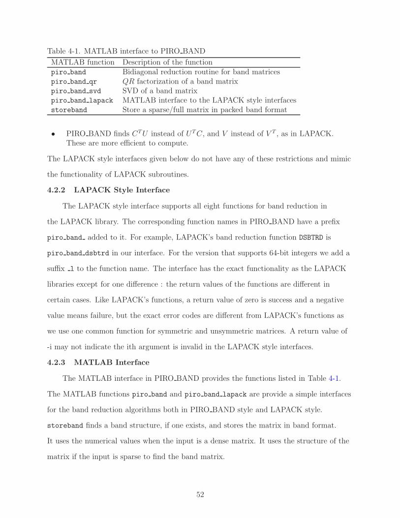
PIRO BAND is a library with both MATLAB and C interfaces for band reduction.
The C interfaces are described in Sections 4.2.1 and 4.2.2. The MATLAB interfaces are
described in Section 4.2.3.
PIRO BAND accepts general sparse and dense matrices in the MATLAB interface.
The C library requires the input matrices to be in the packed band format. Given an
m-by-n matrix A with bl diagonals in the upper triangular side and bu diagonals in the
upper triangular side, the packed band data structure is of the size (bl + bu + 1)-by-n
where entry A(i, j) is stored in entry (i − j + bu, j). The MATLAB interface will accept
49
both sparse and dense matrices and convert them to band form using the structure of the
matrix when the input is sparse and the numerical values when the input is dense.
PIRO BAND’s C interface and the MATLAB interface support real and complex
matrices. Complex matrices are expected to be stored in the C99 style complex format
where the real and imaginary part of every entry is stored in consecutive memory
locations. We do not require C99 for compiling and using the libraries, but the test
coverage for the library requires C99 support. PIRO BAND C libraries do not support
complex matrices where the real and imaginary part are stored in separate arrays.
4.2.1 PIRO BAND Interface
The primary function for band reduction is piro band reduce. There are eight
different versions of this function for all the combinations of double precision and single
precision arithmetic, real and complex matrices and 32-bit and 64-bit integers. The eight
versions of the functions can be defined using the following template.
piro_band_reduce_<x><y><z>
x := ’d’ | ’s’ (for double or single precision)
y := ’r’ | ’c’ (for real of complex matrices)
z := ’i’ | ’l’ (for 32-bit or 64-bit integers)
For example, piro band reduce dri, is the function name for using double precision
arithmetic for reducing a real band matrix with 32-bit integers. The prototype for this
function is
int piro_band_reduce_dri
(
int blks[], int m, int n, int nrc, int bl, int bu, double *A,
int ldab, double *B1, double *B2, double *U, int ldu, double *VT,
int ldv, double *C, int ldc, double *dws, int sym
)
The piro band reduce functions destroy their input matrix A as they reduce it
to bidiagonal/tridiagonal form. The two diagonals are returned on success. The plane
rotations are accumulated in the right and left only if they are required. We do not
provide a separate interface for symmetric and unsymmetric matrices. Instead, we use an
50
input flag to differentiate between the two: the last parameter to the function sym is true
for a symmetric matrix.
All the eight versions of the piro band reduce functions require an optional block
size (blks) and a workspace (dws) as a parameter. blks is an array of size four where
the first two entries specify the number of columns (cu) and rows (ru) in the block for the
reducing the super diagonals. The next two entries in blks specify the number of rows
(rl) and columns (cl) in the block for reducing the subdiagonals. The number of rows and
columns in the blocks are limited by
cu + ru < u (4–1)
cl + rl ≤ l (4–2)
The block size can be different for the reductions in the upper triangular and lower
triangular part. The work space should be two times the maximum of the two block
sizes. The recommended block size is provided by the function piro band get blocksize
in architectures with 32-bit integers. The 64-bit version of the function has a suffix l.
PIRO BAND gets the recommended block size and allocates the required work space if
they are not passed to the library. See the PIRO BAND user guide [Rajamanickam and Davis
2009c] for the exact prototype and the description of the parameters. The selection of the
default block size is explained in Section 4.3.1.
The PIRO BAND interface has some differences from the LAPACK style interface we
provide (described in Section 4.2.2), but it is faster as it will avoid a few transposes. The
major differences between the two interfaces are :
• PIRO BAND requires the upper bandwidth to be at least one.
• For symmetric matrices PIRO BAND requires the upper triangular part to bestored.
51
Table 4-1. MATLAB interface to PIRO BAND
MATLAB function Description of the functionpiro band Bidiagonal reduction routine for band matricespiro band qr QR factorization of a band matrixpiro band svd SVD of a band matrixpiro band lapack MATLAB interface to the LAPACK style interfacesstoreband Store a sparse/full matrix in packed band format
• PIRO BAND finds CT U instead of UT C, and V instead of V T , as in LAPACK.These are more efficient to compute.
The LAPACK style interfaces given below do not have any of these restrictions and mimic
the functionality of LAPACK subroutines.
4.2.2 LAPACK Style Interface
The LAPACK style interface supports all eight functions for band reduction in
the LAPACK library. The corresponding function names in PIRO BAND have a prefix
piro band added to it. For example, LAPACK’s band reduction function DSBTRD is
piro band dsbtrd in our interface. For the version that supports 64-bit integers we add a
suffix l to the function name. The interface has the exact functionality as the LAPACK
libraries except for one difference : the return values of the functions are different in
certain cases. Like LAPACK’s functions, a return value of zero is success and a negative
value means failure, but the exact error codes are different from LAPACK’s functions as
we use one common function for symmetric and unsymmetric matrices. A return value of
-i may not indicate the ith argument is invalid in the LAPACK style interfaces.
4.2.3 MATLAB Interface
The MATLAB interface in PIRO BAND provides the functions listed in Table 4-1.
The MATLAB functions piro band and piro band lapack are provide a simple interfaces
for the band reduction algorithms both in PIRO BAND style and LAPACK style.
storeband finds a band structure, if one exists, and stores the matrix in band format.
It uses the numerical values when the input is a dense matrix. It uses the structure of the
matrix if the input is sparse to find the band matrix.
52
The function piro band svd computes the singular value decomposition of a band
matrix. It can compute both the full and economy singular value decomposition of the
band matrix. The usage also supports finding only the singular values. The singular
value decomposition function uses our band reduction algorithm to reduce the matrix
to bidiagonal/tridiagonal form. It then uses LAPACK (bundled within MATLAB)
to diagonalize bidiagonal/tridiagonal matrix to compute the singular values. The
piro band svd function computes the economy singular value decomposition in three
steps. It uses the simplicial left-looking QR factorization to compute an upper triangular
banded matrix R. It then reduces R using the bidiagonal reduction algorithm and the
LAPACK diagonal reduction algorithm.
piro band qr provides a MATLAB interface to the left-looking band QR factorization.
It provides an option to find both Q and R and an option to find the Householder vectors
instead of Q. See PIRO BAND user guide [Rajamanickam and Davis 2009c] for the exact
usage of all these functions.
4.3 Performance Results
All the performance results here were taken on a machine with eight dual core 2.2
GHz Opteron processors with 64GB of main memory. We used MATLAB 7.6.0.324
(R2008a). PIRO BAND was compiled with gcc version 4.1.1 with the option -O3.
4.3.1 Choosing a Block Size
Choosing the right block size for different machines is a difficult problem. We provide
a function in C that estimates the recommended block size based on the number of
floating point operations. The function will not optimize the block size for any specific
hardware or compiler. The simple rule is to use a block size of 8-by-8 when the required
flops is less than 1010 and the block size of 32-by-32 otherwise. This is our default block
size. The function piro band get blocksize uses 6kn2 as an estimate for the number of
FLOPS for the band reduction algorithm. Figure 4-1 uses the estimated FLOPS for the
x-axis.
53
108
109
1010
1011
1012
0.9
1
1.1
1.2
1.3
1.4
1.5
1.6
1.7
1.8PIRO_BAND Relative Block Size Performance
FLOPS
blk
time/
defa
ult t
ime
blk=rowblk=8blk=16blk=32blk=64
Figure 4-1. Performance of piro band reduce for different block sizes
To verify this simple block size selection we compare five different options : an entire
row as the block, block sizes of 8-by-8, 16-by-16, 32-by-32 and 64-by-64. When the entire
row is used as the block the blocked reduction algorithm does exactly the same amount
of flops as Schwarz’ row reduction method. It does more flops (by a constant factor) for
the other four blocking sizes. Figure 4-1 shows the performance comparison of various
block sizes in relation to the default block size. When the flop count is smaller 8-by-8 is
the ideal block size. As the flops reach 1010 there are a few cases where 16-by-16 is better,
but 32-by-32 is ideal when the flop count is higher. Note that except when choosing the
entire row as the block, all the other block sizes perform within 30% of the default size.
We can also see that 64-by-64 is almost as good as 32-by-32 when we do lot of floating
54
108
109
1010
1011
1012
0.8
0.9
1
1.1
1.2
1.3
1.4
1.5
1.6
1.7
1.8PIRO_BAND Relative Block Size Performance
FLOPS
blk
time/
defa
ult t
ime
blk=row
blk=8
blk=16
blk=32
blk=64
Figure 4-2. Performance of piro band reduce for different block sizes
point operations. There can be a cut-off point where 64-by-64 may start performing better
than 32-by-32. We chose to leave the default at 32-by-32 and let the user experiment for
their common problem sizes.
As the block sizes are platform dependent we repeated this experiment on a machine
with a a 3.2 GHz Pentium 4 and 4 GB of memory. The results are shown in Figure 4-2.
Though the performance of various block sizes are somewhat different from Figure 4-1 the
default block size is never more than 15% worse than the best block size which in this case
is 16-by-16 for some problems.
55
Table 4-2. PIRO BAND svd vs MATLAB dense svd
N Bandwidth PIRO BAND SVD MATLAB DENSE SVD(seconds) (seconds)
The rightmost corner is column 13 and the leftmost corner is column 4. The
rightmost column entry is (7, 13). The rightmost corner entry is marked with a R and
the leftmost corner is marked with a L. Columns 14 . . . 16 are called the rubble.
5.2.2 Mountain, Slope and Sink
The mountainview profile has special properties that we can exploit while doing
the reduction. The following definitions apply both to the mountainview and the skyline
profiles, but are defined using the mountainview profile of R. We classify every column
of the mountainview profile in the range 3 . . . n as one of the following 3 cases: mcolumn,
sink or slope.
Definition 5.10 (Mcolumn). A column j is an mcolumn (a column in a mountain) if
trow(j − 1) = trow(j) in the mountainview profile of R.
62
Slope
mcolumn
Sink
Mountain
X X X X X
X X X X X X X
X X X X X X
X X X X X
X X X X X
X X X X X
X X X X X X X
X X X X X X
X X X X X X
X X X X X
X X X X
X X X
X X
X
XX
X X X XXX
Mountainview(R)
Figure 5-5. Types of columns in the mountainview profile
Definition 5.11 (Mountain). A set of mcolumns all with the same top row value in the
mountainview profile of R.
Definition 5.12 (Slope). A column j is a slope if trow(j − 1) + 1 = trow(j) in the
mountainview profile of R.
Definition 5.13 (Sink). A column j is a sink if trow(j − 1) + 1 < trow(j) in the
mountainview profile of R.
Definition 5.14 (Base height of a mountain). Base height of a mountain is the height of
the mcolumn with the smallest index in that mountain in the mountainview profile of R.
Figure 5-5 illustrates the definitions with the mountainview profile of R matrix we
used in Section 5.2.1. A sample mcolumn, slope and sink are marked in the figure along
with one of the mountains. There are three mountains in the mountainview profile of
R including columns {4, 5, 6, 7}, {9, 10} and {12, 13}. The base height of each of the
mountain is 2, 5 and 5 respectively. Note that we do not define column 3 to be part of
the first mountain even when it shares the trow value with columns 4 . . . 7. Column 3 is
defined as a slope instead.
There are a few properties that follow directly from the definition. In the mountainview
profile:
63
ii−1
ecol(i−1)
. .
. .
X X
X X
X X
X X
X
XX
..
X X ?
X X L
Figure 5-6. End column lemma
• A corner will always be an mcolumn.
• The rightmost corner is in the rightmost mountain.
• For any column j and its top row i = trow(j), rotating rows i and i − 1 generatesmore than one fill if j is an mcolumn, at least one fill that cannot be chasedimmediately if j is a sink and one fill that can be chased if j is a slope.
Mcolumn height property. In a mountainview profile the height of the columns
in any mountain monotonously increases from the lowest numbered column to the highest
numbered column.
Proof. Every column j in the mountain has the same trow(j) value from the
definition. The smallest numbered column sets the base height. As j increases for every
column in the mountain the height, j − trow(j) increases too.2
5.2.3 Properties of Skyline and Mountainview Profiles
There are potentially more than one corner in the profile of a sparse matrix R that
we can reduce to get a fill in the subdiagonal. Furthermore, the chase to reduce the
subdiagonal fill has to be handled as well. We need to characterize the fill and the profiles
better to arrive at an algorithm for reducing the upper triangular matrix. The following
properties help us do it.
Lemma 1 (End-column lemma). Given the profile of R, ecol(i − 1) ≤ ecol(i) for all i
in the range 2 . . . n.
64
righmost corner
j−1
j
n is a corner. Contradiction !
X X
. .
. .
X X X
X X X X X
X X
X X X X X
X X X X X
X X X X
X X
X X X X
X X X
X X
X
X
X X
XX X
Figure 5-7. Top row lemma
Proof. Assume ecol(i − 1) > ecol(i) for some i in the range 2 . . . n. This means
(i − 1, ecol(i − 1)) (entry marked L in Figure 5-6) is in the profile and (i, ecol(i − 1))
(entry marked ? in Figure 5-6) is not in the profile. From the definition of the profile, if
(i − 1, ecol(i − 1)) is in profile (i, ecol(i − 1)) is in the profile. A contradiction. 2
Lemma 2 (Mountainview lemma). Given the mountainview profile of R, trow(j−1) ≤
trow(j) for all j in the range 2 . . . n.
Proof. The proof is similar to the proof of the End-column lemma. Assume trow(j −
1) > trow(j) for some j in the range 2 . . . n. This means (trow(j), j) is in the profile and
(trow(j), j − 1) is not in the profile. From the definition of the mountainview profile, if
(trow(j), j) is in profile (trow(j), j − 1) is in the profile. A contradiction. 2
Lemma 3 (Top-row lemma). If k is the rightmost corner then trow(j − 1) < trow(j)
for all j in the range k + 1 . . . n.
Proof. Assume that there exists a pair of columns j−1 and j such that trow(j−1) ≥
trow(j) and j > k. If j = k + 1 we get a straightforward contradiction as k cannot be a
corner if trow(k) ≥ trow(k + 1). If j = n and trow(j − 1) ≥ trow(j) then n will be the
rightmost corner. A contradiction.
65
righmost corner
i
i−1
ecol(i−1)
ecol(i)j
X X
. .
. .
X X X
X X X X X
X X
X X X X X
X X X X X
X X X X
X X
X X X X
X X X
X X
X
XX X
Figure 5-8. Rubble row lemma
We still have the case of j in the range k + 2 . . . n − 1. As we assumed trow(j −
1) ≥ trow(j), to avoid j being a corner (and result in a contradiction immediately)
trow(j) ≥ trow(j + 1) must be true. As we proceed from columns j − 1 . . . n we have the
All the inequalities in the above equation should be equalities as height(j) cannot increase
as m is the first corner in the range 3 . . . j−1. If the heights of all the columns in the range
p − 1 . . . j remain the same, i.e the inequalities above are all equalities, then height(j) =
height(j − 1) resulting in a corner in j which is to the right of the rightmost corner m. A
contradiction. 2
Theorem 5.3 shows that if we reduce the rightmost corner always and chase the
fill then we reduce the rightmost mountain and the rubble to a height less than the
base height of the rightmost mountain before we reduce any corner from the left of the
mountain. In short, always reducing the rightmost corner actually is a method that always
reduces the rightmost mountain. We did not use any of the special properties of the
mountainview profile here except the definitions. Theorem 5.3 holds for the skyline profile
with a small change : All the columns in the range j . . . n will have height less than or
equal to the original height of j − 1. The proof remains the same.
This shows one can effectively block the reduction in the mountainview profile. The
size of the block depends on the size of the mountain. The size of the block is dynamic
since the size of the mountain changes. Figure 5-10(b) shows the block and first four
corners that will be reduced together as one block. Note that though the first three
corners are in the mountain, one column in the rubble contributes to the block. Figure
72
5-10(c) shows the second mountain and the three corners that will be reduced as one
block. There is no rubble column that can be added to this block for the reduction. The
corner entries 1 . . . 7 in these figures are chosen in that order because the rightmost corner
method would have chosen them too.
The blocking in the skyline profile is a little more trickier. It is presented in detail in
Section 5.3.2. We see all the algorithms to reduce the sparse R in Section 5.3.
5.3 Bidiagonalization Algorithms
The simplest algorithm to reduce R uses the result of Theorem 5.1 that reducing the
rightmost corner results in zero or one fill. Algorithm 5.1 reduces the rightmost corner and
uses a plane rotation to reduce the subdiagonal fill. This algorithm does not use blocking
or pipelining.
Algorithm 5.1 Rightmost corner algorithm for bidiagonalization
1: Find all the corners from 1 . . . n and push them into a stack.2: while there are more corners do3: Pop the rightmost corner k4: Reduce the rightmost corner entry by applying a rotation between columns k and
k − 1.5: Reduce the fill by applying a rotation between rows k and k − 1.6: Inspect columns k−1, k+1, and ecol(k) for new corners and push the new corners to
stack.7: end while
We do not deal with the fill explicitly in this algorithm. If the fill in column ecol(k)
can be chased it will be the new rightmost corner and chased. If the fill can not be
chased then we reduce the next rightmost corner. Given a band matrix in sparse form the
rightmost corner algorithm reduces it exactly like Schwarz’s diagonal reduction method
(Algorithm 2.2). Just like the diagonal reduction method the rightmost corner algorithm is
not blocked, does more work and results in poor performance.
When the rightmost corner method is similar to the diagonal reduction method
[Schwarz 1963] it is natural to look for a method to reduce R like the Schwarz’s row
reduction method[Schwarz 1968]. We need to choose the leftmost corner and reduce it to
73
mimic Schwarz’s row reduction method. However, the leftmost corner may generate more
than one fill in the profile. We can alter the definition to always rotate a ‘valid corner’,
one that generates only one fill, and give preference to the leftmost valid corner. Though
we can prove progress in this case, and that there exists at least one valid corner always
- the rightmost corner, the leftmost corner algorithm does not work very well in practice.
The fill generated and accessing columns in a complex fashion lead to poor performance.
It does not have the nice properties of the rightmost corner algorithm, so blocking the
leftmost corner method turns out to be difficult. We do not describe the leftmost corner
algorithm in detail here. The idea of the leftmost corner algorithm was fully given shape
in [Davis and Golub 2003].
5.3.1 Blocking in Mountainview Profile
Algorithm 5.2 Blocked rightmost mountain algorithm for mountainviewbidiagonalization
1: Find all the corners from 1 . . . n and push them into a stack.2: while there are more corners do3: Pop the rightmost corner k and find the rightmost mountain4: while there are more corners in the rightmost mountain/rubble do5: Use the (trow(k), k) as an anchor point and find a block in the mountain6: Divide the matrix into blocks based on the block.7: Find column rotations to reduce the corners in the block and apply them to the
columns in this block8: while there are column rotations do9: Apply column rotations to C-block.
10: Apply column rotations to D-block in a pipelined order and generate rowrotations to chase the fill.
11: Apply row rotations to R-block.12: Apply row rotations to F-block in a pipelined order and generate column
rotations to chase the fill wherever possible.13: Readjust the four blocks to continue the chase14: end while15: end while16: end while
A blocked algorithm can be derived from the rightmost mountain theorem ( 5.3) and
Theorem 5.2 to reduce the mountainview profile of R. The basic idea is to reduce the
74
mountainview profile one mountain at a time starting from the rightmost mountain. When
the number of columns in the mountain becomes too large we can limit the block size and
reduce one mountain in multiple steps.
We choose the rightmost corner entry as our anchor point for our blocked rightmost
mountain algorithm and find a block around that anchor point. This block serves as our
seed block to find all the entries that can be reduced in one step. Finding a block around
the anchor point in the mountainview profile is similar to finding the block in the band
reduction algorithm in Chapter 3. Once we have the seed block defined we can reduce
the corners within the seed block, divide the rest of the matrix into blocks and pipeline
the plane rotations similar to the algorithms in Sections 3.2 and 3.3, but there are
some differences as we operate on a sparse R. When we chase the fill some fill is chasable
and some fill is left behind, so the indexing is not as smooth as it was in the band case.
Instead, we need to store the indices of columns and rows along with the plane rotations
and apply it to the corresponding columns/rows.
Algorithm 5.2 reduces the mountainview profile in a blocked fashion by reducing
the rightmost mountain in one or more steps depending on the block size and the size
of the mountain. The blocked rightmost mountain algorithm establishes that blocking
and pipelining is possible to reduce a sparse upper triangular R. However, it operates on
mountainview profile of R and the size of the mountainview profile is quite large. The
blocked algorithm must work on the skyline profile to be of practical use.
5.3.2 Blocking in Skyline Profile
Among the theorems we used to arrive at a blocked algorithm for the mountainview
profile Theorem 5.3 and Lemma 6 apply to the skyline profile. But the mcolumn height
property and Theorem 5.2 do not apply to the skyline profile. This means we still reduce
one mountain (the rightmost one) to rubble in the skyline profile when we use the
rightmost corner algorithm, but we cannot consider the entire mountain as one block
75
p k
X X X X
X X X X
X X X
X X X X X
X X X X X
X X
X X X X XX X X X X
X X X X
X X X X X
X X X X
X X X
X X
X
XX
X XXX
••
Figure 5-11. Problem with simple blocking in the skyline profile
as the fill need not be just in the rubble. The fill could be in one of the columns of the
skyline that correspond to the mcolumns of the rightmost mountain.
Say the mcolumns of the rightmost mountain are j . . . k where k is the rightmost
corner. Given the skyline profile, we can find a column p such that j < p < k and a row
rotation of p and p − 1 generates fill in some column less than k, so we avoid columns
that could generate such fill when we find the block. This is shown in Figure 5-11. We
use a different skyline matrix in this figure than the one we have been using so far in this
chapter to illustrate the trouble. There are two corners in the rightmost mountain. When
we reduce the left corner in column p it results in more than one fill in columns k − 1 and
k + 1 (marked as •). This leads us to the problem of finding the right seed block after
finding the anchor point which is the rightmost corner. In the best case it could be the
rightmost mountain and in the worst case it could be just the rightmost corner entry when
no blocking is possible.
The block definitions are the same as in Section 3.2. If k is the rightmost corner
then the first (or least) row in the S-block is trow(k). This is also the trow value for all
the columns in the rightmost mountain. Let us say fcol and lcol define the first and last
columns of the S-block and lrow defines the last row in the S-block. The algorithm to find
the S-block finds the values for fcol, lcol and lrow. The basic idea is that once we select the
rightmost corner entry (trow(k), k) as our anchor point and our S-block with two entries
76
we inspect the columns to the left of it, rows below it and columns to the right of it and
expand the S-block to get a good number of corners to be blocked and reduced together.
However, a few restrictions must be placed on the S-block so that we always limit the fill
to the rubble and we are able to partition the rest of the matrix correctly into blocks.
Algorithm 5.3 Finding the S-block for blocked skyline reduction
1: Set the initial values of lrow to trow(k − 1), fcol to k − 1 and lcol to k.2: Set the initial values for the first row of D-blk to k − 1 and first column of F-blk to
ecol(k − 1).3: Inspect columns to the left of S-block and include columns satisfying the conditions for
S-block.4: Inspect row below the S-block and include row satisfying the conditions for S-block5: Inspect columns to the right of S-block and include columns satisfying the conditions
for S-block.
1. The trow of all the columns in the S-block should be in the S-block. In other wordslrow should be at least equal to the maximum of trow values of all the columns inS-block.
2. The fcol is limited by the least column in the mountain.
3. The S-block and the D-block cannot share a row.
4. The S-block and the F-block cannot share a column.
Condition one avoids the problem shown in Figure 5-11 as we do not do any row
rotations in the S-block we can not create any fill in the mcolumns. Condition two is
not strictly necessary. We can relax it to say fcol is limited by the column trow(k), but
that greatly complicates the block structure, so we restrict the block to the mountain.
Condition three and four ensure we can partition the matrix into blocks correctly. The
algorithm to find the S-block checks for these conditions and increases the block size
to utilize pipelining and caching for performance. The algorithm to find the S-block is
listed in 5.3. Once we find the S-block the algorithm to reduce the skyline is similar
to the blocked rightmost mountain algorithm for mountainview reduction algorithm
(Algorithm 5.2). The algorithm to reduce the skyline is shown in Algorithm 5.4.
77
Algorithm 5.4 Blocked rightmost mountain algorithm for skyline bidiagonalization
1: Find all the corners from 1 . . . n and push them into a stack.2: while there are more corners do3: Pop the rightmost corner k and find the rightmost mountain columns4: while there are more corners in the rightmost mountain/rubble do5: Use the (trow(k), k) as an anchor point and find a block using Algorithm 5.3.6: Divide the matrix into blocks based on the block.7: Find column rotations to reduce the corners in the block and apply them to the
columns in this block8: if there are new corners that got generated which are not within the boundaries
of the seed block then9: push it in the stack for next iteration.
10: end if11: while there are column rotations do12: Apply column rotations to C-block.13: Apply column rotations to D-block in a pipelined order and generate row
rotations to chase the fill.14: Apply row rotations to R-block.15: Apply row rotations to F-block in a pipelined order and generate column
rotations to chase the fill wherever possible.16: Readjust the four blocks to continue the chase17: end while18: end while19: end while
We illustrate the blocked skyline algorithm with an example skyline R in Figure 5-12.
The first S-block as determined by the algorithm to find the S-block is shown in
Figure 5-12(a). All the corners are highlighted and the corner that is going to be reduced
is numbered. Corner 1 results in a swap. Figure 5-12(b) shows the result of the swap with
0s in the swapped corner and the two new corners that were created as a result of the
swap. The three corners 1, 2, 3 in Figure 5-12(a)-(b) are reduced in one step by the skyline
algorithm. The corner numbered 3 is from the rubble but was included in the S-block
to help blocking. Notice that the corresponding block in the mountainview profile was
reduced with four rotations by the mountainview algorithm in Figure 5-10.
Figure 5-12(c) shows the newly created zeros and next S-block for the reduction.
The third S-block is shown in Figure 5-12(d). Column 4 was not included as part of this
S-block even though it is part of the same mountain because it would have created a
78
(d)
(a) (b) (c)
(e) (f)
X X X X
X X X X X 0 0X X X X X 0
X X X X X
X X X X X
X X X X X
X X X X X
X X XX X
X X X X X
X X X X
X X X
X X
X
XX
X X XX
X 7XX
X
X X X X
X X X X X X XX X X X X X
X X X X X
X X X X X
X X X X X
X X X X X 1X X X X X
X X X X X
X X X X X
X X X X
X X X
X X
X
XX
X XXX
X X X X
X X X X X X XX X X X X X
X X X X X
X X X X X
X X X X X
X X X X X 2 0X X 0XX X
X 3X XX
X X X X X
X X X X
X X X
X X
X
XX
X XXX
0
X X X X
X X X X X 5 4X X X X X 6
X X X X X
X X X X X
X X X X X
X X X X X 0X X XX X
X X X X X
X X X X
X X X
X X
X
XX
X XXX
X 0X XX X
X X 9X
X X X X X
X X X X X
X X X X X
X X X X X
X X X X X
X X X X X
X X XX X
X X X X X
X X X X
X X X
X X
X
XX
X X XX
X 0XX X
X
X X X 0X X X X 10
X X X X X
X X X X X
X X X X X
X X X X X
X X X X X
X X XX X
X X X X X
X X X X
X X X
X X
X
XX
X X XX
X XX X
X
Figure 5-12. First three blocks and ten corners of the skyline reduction algorithm
fill in column 5. As corner 7 results in two swaps (corner 8 for the second swap is not
shown) we get two new corners (shown in Figure 5-12(e)) , but the corner in column 5 is
not reduced in the current S-block as column 4 is not in the current S-block. This step is
handled in Line 8 of Algorithm 5.4. We reduce corner 9 and then corner 10 as shown in
Figure 5-12(e)-(f). Corners 7 . . . 10 are part of one step in the blocked reduction.
Note that even though we use the mcolumns to find the possible size of the S-block,
we narrow the S-block in Algorithm 5.3, so the blocks are smaller than the blocks in the
mountainview reduction algorithm. However, we operate on the skyline profile which
is much more economical than the mountainview profile and as a result the number of
operations is reduced.
79
not a sink, a mcolumn
Sink
k
Slope
Figure 5-13. Classification of columns in the skyline profile
In the skyline algorithm the S-block can have more than one corner in it as in the
Figure 5-12(b). This cannot happen in the mountainview profile. Each corner in the
S-block causes at most one fill based on the way we found the S-block, so we can choose
to reduce them in any order. Currently we eliminate the leftmost corner within the block
so that we can reduce the operation count. We call this the rightmost mountain left
corner algorithm. Given a band matrix this algorithm mimics the ‘row mode’ described in
Section 3.5. Instead of choosing the leftmost corner all the time if we choose one rightmost
corner after every c (say 32) leftmost corners we mimic the ‘block mode’ from Section 3.5.
There is an implementation issue we have not addressed in this section so far. The
band reduction Algorithm 3.1 chases all the fill to end of the matrix. On the other
hand the skyline reduction algorithm has to leave some of the fill that is not chasable
in the profile which requires a dynamic data structure. A symbolic factorization for the
skyline reduction that estimates the space requirements for each column is presented in
Section 5.4
5.4 Symbolic Factorization
We use the definitions from Section 5.2.2 to arrive at the symbolic factorization
algorithm. Notice that the definition are using the mountainview profile though they apply
80
k
j
pkk−1
k
k−1
jj−1
j
j−1
sink
pp−1
if ecol(k) = j and trow(j) = k
Figure 5-14. Symbolic factorization of the skyline profile
to both the profiles. Figure 5-13 illustrates the need for using the mountainview profile to
define the mcolumn and sinks in the skyline profile. Column k − 3 in the figure is not a
sink but an mcolumn. We classify it as such because column k − 3 cannot get filled when
we use Algorithm 5.4 for reducing the skyline. It cannot be a sink. We can also write
this as, column j in skyline profile is a sink if and only if trow(j − 1) + 1 < trow(j) and
trow(k + 1 : n) ≥ trow(k).
When we use this classification for the columns in skyline, from the definition of the
corner, any fill in the slope is chasable, any fill in the sink is not chasable and a mcolumn
cannot get a fill when we use the rightmost mountain algorithm for the skyline. We can
then define a fill graph F={V, E} where V = {1 . . . n} are the vertices and edges E. An
edge (i, j) is in E if and only if ecol(i) = j and trow(j) = i. Figure 5-14 illustrates this
graph with a simple example.
Theorem 5.4. When column k is the rightmost corner, reducing the rightmost corner
entry results in one fill in column j if and only if edge (k, j) exists in F .
Proof. We know that from the rightmost corner theorem (Theorem 5.1 there can be
at most one fill in the rubble when you reduce the rightmost corner. We also know from
the rubble column lemma (Lemma 4) and rubble row lemma (Lemma 5 that the fill, if it is
81
there, is in ecol(k) which implies if the fill is in column j then ecol(k) = j. We also know
that the fill is in row k − 1 (as the row rotation is between columns k and k − 1) which
implies that trow(j) = k, so we can say from the definition of the edge (k, j) is present in
F .
On the other hand, if the edge (k, trow(k)) is present then we know ecol(k) = j and
trow(j) = k. We know trow(j − 1) < trow(j) from the top row lemma which ensures
ecol(k − 1) = j − 1. Then a row rotation between rows k and k − 1 has to lead to a fill in
the entry (k − 1, j). 2
Theorem 5.5. If column k is the rightmost corner then reducing the corner and the
resultant chase results in a fill that is not chasable in column q if and only if there is a
sink-free path from k to q in F and column q is a sink.
Proof. If the fill in column q is not chasable then it is a sink by definition. If there
was a fill in column q from the chase, from the fact that rightmost corner algorithm
(Algorithm 5.1) does not handle the fill directly, but the fill itself will be the rightmost
corner at every minor step in the chase (if it is chasable) we can apply Theorem 5.4 to
every minor step so that a path exists from k to q in F . If the path had any other sink
column r then the fill in column r cannot be chased to q, a contradiction, so the path has
to be sink-free.
On the other hand, if there is a sink free path from k to q in F then for all vertices
k, p1, p2, . . . pn, q in the path it is true that ecol(k) = p1, ecol(p1) = p2 until ecol(pn) = q
and trow(q) = pn, trow(pn) = pn−1 until trow(p1) = k. Combining the trow and ecol
values and the fact columns p1, p2, . . . pn have to be slopes (there are no sinks in between),
the fill follows the path and will be the rightmost corner at each minor step and chasable
to q creating a fill there. 2
Theorems 5.4 and 5.5 help us characterize the fill pattern. We define the rightmost
sink as the largest column index for which a column is a sink. The sink helps us in two
ways:
82
1. If we reduce the rightmost corner and follow the path using trow and ecol valuesand reach a sink we have an a fill that is not chasable and the column height has togrow.
2. If the rightmost sink is s, then the columns from s + 1 . . . n cannot grow as long asthe sink remains the same.
A simple symbolic factorization algorithm is to simulate the entire factorization
but without doing any numerical work. As it operates only on trow and ecol values
this algorithm takes only as many as steps as the number of plane rotations which is
considerably less than the actual floating point operations. However, given a band matrix,
which does not need any additional space at all, the symbolic factorization would reduce
the entire matrix symbolically to find that it does not require any space.
The rightmost sink condition gives us a good stopping criterion for the symbolic
factorization. Note that the band matrix has no sinks and if we use it as a stopping
criterion the symbolic factorization stops immediately after finding that there no sinks.
Algorithm 5.5 modifies the simple symbolic factorization to use this stopping criterion.
Algorithm 5.5 Symbolic factorization for the rightmost corner method
1: Find all the corners from 1 . . . n and push them into a stack.2: Inspect all the columns from 1 . . . n and find the rightmost sink. (sr)3: while there are more corners and there exists at least one sink do4: Pop the rightmost corner k5: Follow the path from column k in graph F until a sink (s) or until no fill.6: Inspect columns k − 1, k + 1, for new corners and push the new corners to stack.7: Inspect columns k, k +1, and s, s +1 for sink status and update the rightmost sink if
necessary.8: if rightmost sink (sr) is no longer a sink then9: scan columns sr − 1 . . . 1 until you find the next rightmost sink.
10: end if11: end while
Note that Line 12 in Algorithm 5.5 to maintain the rightmost sink may appear costly,
but from the way the sinks get updated we can show that the cost to find the rightmost
sink is O(n) and amortized cost to update the rightmost sink is O(1). It is easy to see that
the initial cost to find the rightmost sink is O(n) as we check the trow values for all the
83
columns. Note that if the rightmost sink sr is no longer a sink (say if it became a slope)
we scan the columns right-to-left to find the new rightmost sink. If this is the only type of
change to the sinks then we will move back to column 1 with another O(n) cost.
However, as a result of of the fill created by a rotation and the swaps new sinks get
created. A sink created by a swap can not be the rightmost sink. If a new rightmost sink
gets created as result of fill then it has to be in sr + 1. We can then update the rightmost
sink in O(1) time. The move towards n will pay for the move back to 1 again when we do
the right-to-left scan to find the next rightmost sink. We do not maintain a list of all the
sinks. Instead, we test it using the trow data structure every time we need it as we access
the data structure to traverse the fill graph.
Algorithm 5.5 modified the non-blocked rightmost corner method for the symbolic
factorization. We can apply the same changes to the blocked algorithms as well to get a
simple symbolic factorization algorithm for the blocked skyline reduction. Algorithm 5.6
computes a symbolic factorization for the blocked skyline reduction. Note that we have
removed the chase from Algorithms 5.5 and 5.6 as following the path in the fill graph
is equivalent to the chase. The fill from these two algorithms can be different as the the
blocked skyline reduction algorithm will reduce the leftmost corner within the seed block.
5.5 PIRO SKY: Pipelined Plane Rotations for Skyline Reduction
PIRO SKY is the library that implements the sparse bidiagonal reduction algorithms
discussed in this chapter. PIRO SKY stands for PIpelined plane ROtations of sparse
SKYline matrices. PIRO SKY has both a MATLAB and C interface. PIRO SKY works
for real sparse matrices, with native integer (32-bit and 64-bit) support, and double
The MATLAB interface of PIRO SKY finds the singular value decomposition of
sparse matrices using our blocked algorithms. To compute the singular value decomposition
we depend on symrcm [Cuthill and McKee 1969] or the implementations of the GPS
algorithm [Gibbs et al. 1976] for finding a profile reduction ordering for the matrix AT A
84
Algorithm 5.6 Symbolic factorization for the blocked rightmost mountain algorithm forskyline bidiagonalization
1: Find all the corners from 1 . . . n and push them into a stack.2: Inspect all the columns from 1 . . . n and find the rightmost sink. (sr)3: while there are more corners and there exists at least one sink do4: Pop the rightmost corner k and find the rightmost mountain columns5: while there are more corners in the rightmost mountain/rubble do6: Use the (trow(k), k) as an anchor point and find a block using Algorithm 5.3.7: For each corner kc in the S-block follow the path from kc in graph F values until a
sink (s) or until no fill.8: if there are new corners that got generated which are not within the boundaries
of the seed block then9: push it in the stack for next iteration.
10: end if11: Inspect columns k, k +1, and s, s+1 for sink status and update the rightmost sink
if necessary.12: if rightmost sink (sr) is no longer a sink then13: scan columns sr − 1 . . . 1 until you find the next rightmost sink.14: end if15: end while16: end while
and then use that for the column ordering of A. We depend on SPQR [Davis 2009a,b] for
computing the QR factorization. PIRO SKY then reduces the sparse upper triangular
R to bidiagonal form. We can then use LAPACK to reduce the bidiagonal matrix to
diagonal form [Golub and Reinsch 1970; Demmel and Kahan 1990; Deift et al. 1991]. We
provide one interface piro sky svd which does all the above steps to compute the singular
value decomposition. We also provide two custom interfaces for computing the symbolic
factorization of the sparse upper triangular R (piro sky symbolic) and for computing the
bidiagonal reduction itself (piro sky reduce).
piro sky reduce can operate in two modes. In the static mode, it can compute the
symbolic factorization, allocate the required amount of memory and do the reduction in
place. In the dynamic mode, it can allocate the space for the skyline matrix dynamically
and compute the reduction. The dynamic mode is useful when the space required by
the factorization (as computed by the symbolic factorization) is unavailable. PIRO SKY
manages the memory dynamically in the later case and reallocates memory as desired.
85
Table 5-1. MATLAB interface to PIRO SKY
MATLAB function Description of the functionpiro sky reduce Bidiagonal reduction routine for sparse matricespiro sky svd Computes the SVD of a sparse matrixpiro sky symbolic Symbolic factorization for the bidiagonal reduction
Table 5-2. C interface to PIRO SKY
C function Description of the functionpiro sky set common: Initializes PIRO SKY with default values.piro sky allocate symbolic: Allocates the data structure for the
symbolic factorization.piro sky symbolic: Computes the symbolic factorization for a given
sparse matrix.piro sky allocate skyline: Allocates the skyline matrix based on the counts from
symbolic factorization.piro sky sparse to skyline: Converts a compressed column format sparse matrix
to a skyline matrix.piro sky reduce: Computes the bidiagonal reduction of the skyline matrix.piro sky free skyline: Frees space used by the skyline data structure.piro sky free symbolic: Frees space used by the symbolic data structure.
The reduction also accepts an approximate bandwidth and can reduce the skyline matrix
to a band matrix. It then converts the skyline to a band data structure and uses the band
reduction algorithm (PIRO BAND) to compute the bidiagonals.
The symbolic factorization in PIRO SKY computes the column counts required for
sparse skyline matrices. It also reports the total number of plane rotations that would
be required to do the reduction and the number of swaps that would take place. The
swaps which look cheaper because they do not do any floating point work are actually
expensive. When two columns are not adjacent to each other in memory the swap cannot
be done in place and we may not be able to fit one column in the place of another. This
could happen when we skip symbolic factorization and operate in the dynamic mode.
PIRO SKY dynamically reallocates space to continue with the reduction then.
The MATLAB interfaces for PIRO SKY are summarized in Table 5-1. The C
interface to PIRO SKY provides a set of functions. The functions and a brief description
of them are shown in Table 5-2. The C functions are listed in the exact order as they
86
100
101
102
103
0
20
40
60
80
100
120
relative run time, vs. best
num
ber
of m
atric
esPIRO_SKY Relative Performance (profile) n/5
MATLAB svdsPIRO_SKY
100
101
102
103
0
20
40
60
80
100
120
relative run time, vs. bestnu
mbe
r of
mat
rices
PIRO_SKY Relative Performance (profile) n/10
MATLAB svdsPIRO_SKY
Figure 5-15. Performance of PIRO SKY vs MATLAB svds
will be used in an example. The users can set an array of parameters using the data
structures in the C interface to fine tune the performance of PIRO SKY including size of
the work space, block size, static/dynamic memory allocation, elbow room for columns,
approximate bandwidth and functions used to allocate and free memory. PIRO SKY is
not publicly available yet. We plan to make it publicly available as an ACM Transactions
of Mathematical Software collected algorithm.
5.6 Performance Results
We compare our PIRO SKY implementation to svds in MATLAB. MATLAB uses
ARPACK [Lehoucq et al. 1997; Lehoucq and Sorensen 1996] to compute the singular
values of a sparse matrix. As MATLAB svds is not designed compute all the singular
values of a sparse matrix and our algorithm is designed to compute all the singular values
we do not compare them in the case of computing all the singular values. Instead, given a
sparse matrix A of size n-by-n, we compute nk
singular values for various values of k using
87
100
101
102
0
20
40
60
80
100
120
relative run time, vs. best
num
ber
of m
atric
esPIRO_SKY Relative Performance (profile) n/25
MATLAB svdsPIRO_SKY
100
101
102
0
20
40
60
80
100
120
relative run time, vs. bestnu
mbe
r of
mat
rices
PIRO_SKY Relative Performance (profile) n/50
MATLAB svdsPIRO_SKY
Figure 5-16. Performance of PIRO SKY vs MATLAB svds
MATLAB svds and compute all the singular values using our method and compare the
results. This should give a better idea of when we can use the iterative method and when
we can switch to our direct method and compute all the singular values instead.
All the tests were done with double precision arithmetic with real matrices from
the UF sparse matrix collection [Davis 2009c]. We used real matrices with n < 5000.
The performance measurements were done on a machine with 8 dual core 2.2 GHz AMD
Opteron processors and 64GB of main memory. PIRO BAND was compiled with gcc
4.1.1 with the options -O3. We used svds in MATLAB 7.6.0.324 (R2008a).
PIRO SKY was configured to always use the symbolic factorization, allocate the
space for the skyline and operate on a static data structure. Furthermore, we allowed 50%
more space than the original number of non-zeros in R (not in the skyline of R) to get an
approximate bandwidth in R below which most entries lie. We then use the bandwidth in
the symbolic and numerical reduction to reduce the matrix to a band matrix. We then use
PIRO BAND library to reduce the band matrix to bidiagonal form. We use MATLAB’s
88
sparse qr and symrcm for the QR factorization and profile reduction steps. We reduced
the bidiagonal matrix to diagonal form using LAPACK. PIRO SKY’s time to compute the
SVD includes the time to compute all these steps.
The results when we compute n5
and n10
singular values are presented in Figure 5-15.
We use a performance profile to compare the two methods. In both cases PIRO SKY
is faster than MATLAB’s svd for all the matrices and computes all the singular values.
Figure 5-16 shows the results for computing n25
and n50
singular values. When n25
singular
values are computed by the svds the performance of both algorithms are competitive
except in a few matrices where PIRO SKY does not perform very well. When we
compute n50
singular values svds performs better in more than half the matrices and
the performance is similar in the other half of the matrices. To summarize, PIRO SKY
computes all the singular values in the time it takes to compute just 4% of singular values
using svds and does much better when more singular values are required.
89
CHAPTER 6CONCLUSION
The singular value decomposition is a problem that is used in wide range of
applications. We studied this problem for two specific class of matrices : a band matrix
and a sparse matrix. Our major contributions to these problems are:
• We developed a blocked algorithm for band reduction that generates no more fillthan any scalar band reduction method using pipelining. The work space requiredfor our algorithm is much smaller (equal to the size of the block) than the workspace required by competing methods (O(n) to O(nnz)). Our blocked methodsperform slightly more work than the Schwarz’s row reduction method but less thanboth LAPACK and SBR band reduction algorithms. When the plane rotations arenot accumulated, our algorithm is about 2 times faster than SBR and 3.5 timesfaster than LAPACK. Our blocked algorithm manages to balance all the threerequirements, cache utilization, number of floating point operations and work spacerequirement.
• We developed an algorithm to accumulate the plane rotations while utilizing thenon zero structure of U and V for our blocked algorithm. Our algorithm reduces thenumber of plane rotations by half, hence the number of flops in accumulations byhalf, as compared to LAPACK’s accumulation algorithm. When the plane rotationsare accumulated our speed up is about 2x and and 2.5x against LAPACK and SBR.
• We developed a library for band reduction that supports all the required data typeswith both C and MATLAB interfaces. PIRO BAND will be made available as acollected ACM TOMS algorithm.
• We developed the theory for sparse skyline bidiagonal reduction, and both blockedand non-blocked algorithms for the problem. We also developed the theory andthe algorithm for symbolic factorization for the bidiagonal reduction method. Ourbidiagonal reduction method uses efficient sparse data structures and computes allthe singular values of a sparse matrix in the same time it takes for the iterativemethod to compute just 4% of the singular values. It performs far better when moresingular values are required. No prior algorithm exists for efficiently computing allthe singular values of a sparse matrix.
• We developed a library for bidiagonal reduction of sparse matrices and finding thesparse singular value decomposition. PIRO SKY supports both C and MATLABinterfaces. PIRO SKY will be made available as a collected ACM TOMS algorithm.Our library for sparse bidiagonal reduction still does not support complex matrices.Complex support will be part of the library when it is made publicly available.
90
It is not expensive to compute the symbolic factorization algorithms described in
Section 5.4, but a theoretical question still remains open. Given the fill graph F it will
be interesting to compute the symbolic factorization without simulating the rotations
of numerical reduction. However, for all practical purposes our symbolic factorization
algorithm works well.
The techniques to adopt our blocked reduction methods to multicore architectures
is another interesting problem that still remains to be studied. The problem has been
studied in the context of reducing a dense matrix to band form [Ltaief et al. 2009]. The
band reduction algorithm could couple the blocking with the technique of moving the
blocks a fixed distance before reducing the next block, as it was done in [Kaufman 2000]
for single entries. However, the synchronization between the blocks have to be worked out
carefully for adopting the blocked algorithm to multicore architectures. Band reduction in
parallel architectures has been studied for sometime though [Lang 1993, 1996]. Efficient
bidiagonal reduction of the sparse skyline matrix in multicore architectures still remains an
open problem.
91
REFERENCES
Anda, A. A. and Park, H. 1994. Fast plane rotations with dynamic scaling. SIAM J.Matrix Anal. Appl. 15, 1, 162–174.
Anderson, E., Bai, Z., Bischof, C., Blackford, S., Demmel, J., Dongarra, J.,Du Croz, J., Greenbaum, A., Hammarling, S., McKenney, A., and Sorensen,
D. 1999. LAPACK Users’ Guide, Third ed. Society for Industrial and AppliedMathematics, Philadelphia, PA.
Barlow, J. L., Bosner, N., and Drmac, Z. 2005. A new stable bidiagonal reductionalgorithm. Linear Algebra Appl. 397, 35–84.
Berry, M. W. 1992. Large scale sparse singular value decompositions. Inter. J. ofSupercomputer Appl. 6, 1, 13–49.
Berry, M. W., Dumais, S. T., and O.Brien, G. W. 1994. Using linear algebra forintelligent information retrieval. SIAM Rev. 37, 4, 573–595.
Billsus, D. and Pazzani, M. J. 1998. Learning collaborative information filters. InICML ’98: Proc. Fifteenth Inter. Conf. Mach. Learn. Morgan Kaufmann PublishersInc., San Francisco, CA, USA, 46–54.
Bindel, D., Demmel, J., Kahan, W., and Marques, O. 2002. On computing Givensrotations reliably and efficiently. ACM Trans. Math. Soft. 28, 4, 206–238.
Bischof, C. H., Lang, B., and Sun, X. 2000a. Algorithm 807: The SBRtoolbox—software for successive band reduction. ACM Trans. Math. Softw. 26, 4,602–616.
Bischof, C. H., Lang, B., and Sun, X. 2000b. A framework for symmetric bandreduction. ACM Trans. Math. Soft. 26, 4, 581–601.
Blackford, L. S., Demmel, J., Dongarra, J., Duff, I., Hammarling, S., Henry,
G., Heroux, M., Kaufman, L., Lumsdaine, A., Petitet, A., Pozo, R., Rem-
ington, K., and Whaley, R. C. 2002. An updated set of basic linear algebrasubprograms (BLAS). ACM Trans. Math. Softw. 28, 2, 135–151.
Bosner, N. and Barlow, J. L. 2007. Block and parallel versions of one-sidedbidiagonalization. SIAM J. Matrix Anal. Appl. 29, 3, 927–953.
Chan, T. F. 1982. An improved algorithm for computing the singular valuedecomposition. ACM Trans. Math. Soft. 8, 1, 72–83.
Cuthill, E. and McKee, J. 1969. Reducing the bandwidth of sparse symmetricmatrices. In Proc. 1969 24th Nat. Conf. ACM, New York, NY, USA, 157–172.
92
Davis, T. A. 2009a. Algorithm 8xx: SuiteSparseQR, a multifrontal multithreaded sparseQR factorization package. Submitted to ACM Trans. Math. Softw., Retrieved October7, 2009 from http://www.cise.ufl.edu/~davis/.
Davis, T. A. 2009b. Multifrontal multithreaded rank-revealing sparse QRfactorization. Submitted to ACM Trans. Math. Softw., Retrieved October 7, 2009from http://www.cise.ufl.edu/~davis/.
Davis, T. A. 2009c. The University of Florida sparse matrix collection.Submitted to ACM Trans. Math. Softw., Retrieved October 7, 2009 fromhttp://www.cise.ufl.edu/~davis/.
Davis, T. A., Gilbert, J. R., Larimore, S. I., and Ng, E. G. 2004a. Algorithm 836:COLAMD, a column approximate minimum degree ordering algorithm. ACM Trans.Math. Softw. 30, 3, 377–380.
Davis, T. A., Gilbert, J. R., Larimore, S. I., and Ng, E. G. 2004b. A columnapproximate minimum degree ordering algorithm. ACM Trans. Math. Softw. 30, 3,353–376.
Davis, T. A. and Golub, G. H. 2003. Personal communications.
Deerwester, S., Dumais, S. T., Furnas, G. W., Landauer, T. K., and Harsh-
man, R. 1990. Indexing by latent semantic analysis. J. Amer. Soc. Inf. Sci. 41,391–407.
Deift, P., Demmel, J., Li, C., and Tomei, C. 1991. The bidiagonal singular valuedecomposition and hamiltonian mechanics. SIAM J. Numer. Anal 28, 1463–1516.
Demmel, J. and Kahan, W. 1990. Accurate singular values of bidiagonal matrices.SIAM J. Sci. Stat. Comput 11, 873–912.
Dongarra, J. J., Du Croz, J., Hammarling, S., and Duff, I. S. 1990. A set oflevel 3 basic linear algebra subprograms. ACM Trans. Math. Softw. 16, 1, 1–17.
Drineas, P., Kannan, R., and Mahoney, M. W. 2004. Fast monte carlo algorithmsfor matrices II: Computing a low-rank approximation to a matrix. SIAM J. Comp. 36,2006.
Gentleman, W. M. 1973. Least squares computations by Givens transformationswithout square roots. IMA J. Appl. Math. 12, 329–336.
Gibbs, N. E., Poole, William G., J., and Stockmeyer, P. K. 1976. An algorithmfor reducing the bandwidth and profile of a sparse matrix. SIAM J. Numer. Anal. 13, 2,236–250.
Givens, W. 1958. Computation of plane unitary rotations transforming general matrix totriangular form. J. SIAM 6, 1, 26–50.
Goldberg, K., Roeder, T., Gupta, D., and Perkins, C. 2001. Eigentaste: Aconstant time collaborative filtering algorithm. Info. Retrieval 4, 2, 135–151.
Golub, G. H. and Kahan, W. 1965. Calculating the singular values and pseudo-inverseof a matrix. SIAM J. Numer. Anal. 2, 2, 205–224.
Golub, G. H. and Reinsch, C. 1970. Singular value decomposition and least squaresolutions. Numer. Math. 14, 5, 403–420.
Golub, G. H. and van Loan, C. F. 1996. Matrix Computations, 3rd ed. The JohnsHopkins University Press.
Hager, W. W. 2002. Minimizing the profile of a symmetric matrix. SIAM J. Sci.Comput. 23, 5, 1799–1816.
Hammarling, S. 1974. A note on modifications to the Givens plane rotation. IMA J.Appl. Math. 13, 215–218.
Kaufman, L. 1984. Banded eigenvalue solvers on vector machines. ACM Trans. Math.Softw. 10, 1, 73–85.
Kaufman, L. 2000. Band reduction algorithms revisited. ACM Trans. Math. Soft. 26, 4,551–567.
Kolda, T. G. and O’leary, D. P. 1998. A semidiscrete matrix decomposition forlatent semantic indexing in information retrieval. ACM Trans. on Inf. Syst. 16, 322–346.
Koren, Y. 2008. Factorization meets the neighborhood: a multifaceted collaborativefiltering model. In KDD ’08: Proc. 14th ACM SIGKDD Int. Conf. Knowledge DiscoveryData Min. ACM, New York, NY, USA, 426–434.
Lang, B. 1993. A parallel algorithm for reducing symmetric banded matrices totridiagonal form. SIAM J. Sci. Comput. 14, 6, 1320–1338.
Lang, B. 1996. Parallel reduction of banded matrices to bidiagonal form. ParallelComput. 22, 1, 1–18.
Larsen, R. M. 1998. Lanczos bidiagonalization with partial reorthogonalization.Retrieved October 7, 2009 from http://soi.stanford.edu/~rmunk/PROPACK/.
Lehoucq, R. and Sorensen, D. C. 1996. Deflation techniques for an implicitlyre-started arnoldi iteration. SIAM J. Matrix Anal. Appl 17, 789–821.
Lehoucq, R. B., Sorensen, D. C., and Yang, C. 1997. ARPACKusers’ guide: Solution of large scale eigenvalue problems with implicitlyrestarted Arnoldi methods. Retrieved October 7, 2009 fromhttp://www.caam.rice.edu/software/ARPACK/UG/ug.html.
Ltaief, H., Kurzak, J., and Dongarra, J. 2009. Parallel band two-sided matrixbidiagonalization for multicore architectures. IEEE Trans. Parallel and Dist. Sys. (toappear), Retrieved October 7, 2009 from http://icl.cs.utk.edu/~ltaief/.
Murata, K. and Horikoshi, K. 1975. A new method for the tridiagonalization of thesymmetric band matrix. Infor. Proc. Japan 15, 108–112.
Paterek, A. 2007. Improving regularized singular value decomposition for collaborativefiltering. In Proc. KDD Cup and Workshop.
Pryor, M. H. 1998. The Effects of Singular Value Decomposition on CollaborativeFiltering. Tech. Rep. PCS-TR98-338, Dartmouth College, Computer Science, Hanover,NH. June.
Rajamanickam, S. and Davis, T. A. 2009a. Blocked band reduction for symmetricand unsymmetric matrices. To be submitted to ACM Trans. Math. Softw., RetrievedOctober 7, 2009 from http://www.cise.ufl.edu/~srajaman/.
Rajamanickam, S. and Davis, T. A. 2009b. PIRO BAND: Pipelined plane rotationsfor blocked band reduction. To be submitted to ACM Trans. Math. Softw., RetrievedOctober 7, 2009 from http://www.cise.ufl.edu/~srajaman/.
Rajamanickam, S. and Davis, T. A. 2009c. PIRO BAND user guide. RetrievedOctober 7, 2009 from http://www.cise.ufl.edu/~srajaman/.
Ralha, R. 2003. One-sided reduction to bidiagonal form. Linear Algebra Appl. 358, 1-3,219–238.
Reid, J. K. and Scott, J. A. 1998. Ordering symmetric sparse matrices for smallprofile and wavefront. Tech. Rep. RAL-TR-98-016, Rutherford Appleton Laboratory.
Reid, J. K. and Scott, J. A. 2002. Implementing Hager’s exchange methods formatrix profile reduction. ACM Trans. Math. Softw. 28, 4, 377–391.
Rutishauser, H. 1963. On Jacobi rotation patterns. Proc. of Symp. in Appl. Math. 15,219–239.
Sarwar, B., Karypis, G., Konstan, J., and Riedl, J. 2002. Incremental singularvalue decomposition algorithms for highly scalable recommender systems. In Fifth Int.Conf. Comput. Inf. Sci. 27–28.
Schwarz, H. R. 1963. Algorithm 183: Reduction of a symmetric bandmatrix to triplediagonal form. Commun. ACM 6, 6, 315–316.
Schwarz, H. R. 1968. Tridiagonalization of a symmetric band matrix. Numer.Math. 12, 4, 231–241.
Smith, B. T., Boyle, J. M., Dongarra, J., Garbow, B. S., Ikebe, Y., Klema,
V. C., and Moler, C. B. 1976. Matrix Eigensystem Routines - EISPACK Guide,Second Edition. Lecture Notes in Computer Science, vol. 6. Springer.
Stewart, G. W. 1976. The economical storage of plane rotations. Numer. Math. 25,137–138.
Sun, J., Xie, Y., Zhang, H., and Faloutsos, C. 2008. Less is more: Sparse graphmining with compact matrix decomposition. Stat. Anal. Data Min. 1, 1, 6–22.
Trefethen, L. N. and Bau III, D. 1997. Numerical Linear Algebra, 1st ed. Society forIndustrial and Applied Mathematics.
Van Loan, C. and Bischof, C. 1987. The WY representation for products ofhouseholder matrices. SIAM J. Sci. Stat. Comput. 8, 1.
Wall, M., Rechtsteiner, A., and Rocha, L. 2003. Singular value decomposition andprincipal component analysis. In A practical Approach to Microarray Data Analysis,D. P. Berrar, W. Dubitzky, and M. Granzow, Eds. 91–109.
96
BIOGRAPHICAL SKETCH
Siva Rajamanickam’s research interests are in sparse matrix algorithms. Specifically,
he works on direct methods for sparse eigen value and singular value decompositions. He
has also worked on band reduction methods and ordering methods for sparse Cholesky
and sparse LU factorizations. He is one of the authors of CCOLAMD (Constrained
Column Approximate Minimum Degree Ordering) library which is part of the CHOLMOD
(Cholesky Modification) package. He was also part of the development teams in Sun