Abstract This paper describes an efficiently computational method for dynamics sim-ulating of planar multibody system with flexible beams undergoing large deformationsby combining the absolute nodal coordinate formulation (ANCF) and the transfer matrixmethod (TMM). Firstly, according to ANCF and the geometrically nonlinear theory, thetwo-dimensional shear-deformable beam element and its dynamic equations of motion arepresented. Then according to TMM and the dynamic equations of beam elements, by defin-ing the new state vectors and deducing the new transfer equations of elements, an efficientcomputational method named as ANC–TMM, is presented for dynamics of planar multibodysystem with flexible beams undergoing large deformations. Compared with the ordinary dy-namics methods, the proposed method combines the strengths of TMM and ANCF. It doesnot need the global dynamic equations of system and has the low order of the system ma-trix and high computational efficiency. This method can be extended to solve the nonlineardynamics problems of general flexible multibody systems undergoing large deformations.Formulations as well as a numerical example of a flexible four-bar linkage mechanism aregiven to validate the method.
Keywords Multibody system · Geometric nonlinearity · Computational method ·Shear-deformable beam element · Large rotation
1 Introduction
With high-performance and high-precision demands of complex mechanical systems suchas lightweight robots, precision machinery, aircrafts and vehicles, large scale, low stiffness,and flexibility has emerged as important trends in these fields [1, 2]. The dynamic modelingand efficient computation of flexible multibody systems (FMS) with geometrical nonlinear-ity and large deformation have become more and more important. The traditional floating
B. Rong (B)Nanchang Military Academy, Nanchang 330103, P.R. Chinae-mail: [email protected]
frame of reference formulation is currently the most widely used approach in flexible multi-body simulations. However, this approach has been limited to small deformation problems,and cannot be used to study the geometrical nonlinearity problems. In order to describethe dynamics of FMS with large deformation, Shabana [3–5] proposed the absolute nodalcoordinate formulation (ANCF). ANCF is a nonincremental finite element method (FEM)for the dynamic analysis of flexible bodies that experience rigid body motion and large de-formation. The use of coordinates that are referred to an inertial frame leads to a constantmass matrix and, as a consequence, neither Coriolis nor centrifugal terms appear in theequations of motion [6–8]. Compared to the floating frame of reference formulation, theANCF leads to an exact modeling of dynamics of FMS with large deformation. However,when studying FMS dynamics by using ordinary ANCF, we often have to face the followingproblems [7]. (1) It is necessary to develop the global dynamic equations of system, and theglobal dynamic equations of system are usually highly nonlinear. They are the differentialequations or differential-algebra equations. (2) The orders of the involved system matricesincrease together with the number of the system degrees of freedom (DOF). ANCF must usea large number of nodes, which results in the high orders of matrices in the global dynamicequations and extreme computational cost. Whereas the accurate, high-efficient demandsof dynamics prediction and control have become more and more important in modern engi-neering fields, how to improve the computational efficiency of ANCF, is an urgently difficultproblem in the field of FMS dynamics.
In order to improve the computational efficiency of ANCF, García-Vallejo [8] used someinvariant sparse matrices for evaluating the elastic forces, the elastic energy, and the Jacobianof the elastic forces. Then the stiffness matrix can be transformed into the sum of two matri-ces: a constant one and a coordinate-dependent one whose components are quadratic formsof the nodal coordinate vector. Gerstmayr [9] and Liu [10] proposed an efficient ANCF byusing the first kind of Piola–Kirchhoff stress tensor to deduct the elastic forces and their Ja-cobians. Based on the Cholesky decomposition, Yakoub [11] expressed the absolute nodalcoordinates in terms of the generalized Cholesky coordinates. In this method, the inertiamatrix associated with the Cholesky coordinates is the identity matrix and, therefore, anoptimum sparse matrix structure can be obtained for the augmented multibody equations ofmotion, and the computational efficiency can be improved. Chijie [12] proposed a parallel al-gorithm to reduce the computational time of dynamic and thermal analysis of flexible struc-tures in orbit. Although these methods can improve the computational efficiency of ANCF tosome extent, they do not change the fact that the global dynamic equations based on ANCFhave high orders of matrices and, therefore, the computational cost is still considerably large.
The classical transfer matrix method (TMM) [13], which has the advantages of beingwithout the system global dynamic equations, high programming, low system matrix order,and high computational efficiency, has been used extensively in structure mechanics and ro-tor dynamics. By combining the TMM with the numerical integration procedure, a discretetime TMM was developed for structure dynamics of a time variant system in [14]. By com-bining the FEM and TMM, Dokanish [15] proposed the FE-TMM, which can improve thecomputational speed of pure FEM greatly. Other researchers, such as Loewy [16], Xue [17],and Rong [18] studied and improved the FE-TMM in different aspects. Rui and Rong [19,20] presented the discrete time TMM of a multibody system to study the dynamics prob-lems of FMS with small deformation. The above advantages of TMM provide a possibilityfor efficient dynamic modeling of large flexible multibody systems.
In this paper, by combining the ANCF and TMM, a new efficient computational methodnamed as ANC–TMM is presented for dynamics simulating of planar multibody systemwith flexible beams undergoing large deformations. Firstly, according to ANCF and the ge-ometrically nonlinear theory, the two-dimensional shear-deformable beam element and its
Efficient dynamics analysis of large-deformation flexible beams by using
dynamic equations of motion are presented. Then by using these dynamic equations of beamelements and defining new state vectors, an improved TMM is introduced to study the dy-namics modeling and simulation of planar multibody system with flexible beams undergoinglarge deformations. Compared with the ordinary dynamics methods, the proposed methodcombines the strengths of TMM and ANCF. It does not need the global dynamic equationsof system and has the low order of system matrix and high computational efficiency. Thismethod can be extended to solve the nonlinear dynamics problems of general FMS undergo-ing large deformations. Formulations as well as a numerical example of a flexible four-barlinkage mechanism are given to validate the method.
This paper is organized as follows. In order to describe the proposed method convenientlyin the following, a dynamics model of a flexible four-bar linkage mechanism, which will betaken as an example in this study is firstly given in Sect. 2. In Sect. 3, a two-dimensionalshear-deformable beam element and its dynamic equations are presented. The general the-orems and steps of the proposed method for dynamics modeling and simulation of pla-nar multibody system with flexible beams undergoing large deformations are introduced inSect. 4. In Sect. 5, the numerical simulation of a flexible four-bar linkage mechanism ob-tained by the proposed method and by ordinary ANCF is given to validate the method. Theconclusions are presented in Sect. 6.
2 Dynamics model of a flexible four-bar linkage mechanism
The study model used is the four-bar mechanism shown in Fig. 1 [4]. This four-bar link-age mechanism can be divided into various components including bodies (a crankshaft, acoupler, and a follower) and hinges. The mechanism is driven by a moment applied to thecrankshaft. From left to right, the components can be regarded as the smooth hinge (0),flexible beam (1), smooth hinge (2), flexible beam (3), smooth hinge (4), flexible beam (5),and smooth hinge (6). Each flexible beam can be divided into some two-dimensional shear-deformable beam elements presented in the following section. The right-handed Cartesiancoordinate system oxy is used to denote the inertial reference frame. In the following sec-tions, taking this flexible four-bar linkage mechanism as an example, an efficiently ANC–TMM is firstly presented to study the dynamics of planar multibody system with flexiblebeams undergoing large deformations. However, the proposed method can also be carriedover in a straightforward manner to other FMS with geometric nonlinearities moving in aplane or space.
3 Two-dimensional shear-deformable beam element and its dynamic equations
In this section, the two-dimensional shear-deformable beam element [5, 7] and its dynamicequations of motion are presented based on the ANCF and the geometrically nonlinear the-ory. As shown in Fig. 2, this beam element has two nodes, and each node has six nodal
Fig. 1 Dynamics model of aplanar four-bar linkagemechanism
B. Rong
Fig. 2 Two-dimensionalshear-deformable beam elementbetween before and afterdeformation
coordinates, which are all defined in the inertial reference frame. The right-handed Carte-sian coordinate system oexeye , which has one of its axes passes through two nodes of thebeam element, is used to denote the local element reference frame. The global position vec-tor of an arbitrary point P in the beam element can be expressed as
rP = [xP yP ]T = S(x ′, y ′)δe (1)
here (xP , yP ) and (x ′, y ′) are the position coordinates of the point P with respect to theinertial and the local element reference frame, respectively. S and δe are the global elementshape function and the element nodal coordinate vector, respectively.
here E is the Young’s modulus of elasticity, and γ is the Poisson’s ratio of the beam material.The strain energy of the beam element can be expressed as
Ue = 1
2
∫
Ve
(σxxεxx + σyyεyy + 2σxyεxy)dVe (9)
Only considering the distributed exterior force f, according to the Lagrange equation, onecan obtain
Me δe + Keδe = Fe + Pe (10)
where Ke is the stiffness matrix of the beam element. Fe is the generalized external forceof the beam element. Pe is the generalized nodal internal force resulting from the connec-tivity of the element with the other elements used in the finite element discretization of thedeformable body.
Ke = Kel + Ken, Kel = −(λ + G)
∫
Ve
(Sx + Sy)dVe
Ken = 1
2(λ + 2G)
∫
Ve
(Sxδeδ
Te Sx + Syδeδ
Te Sy
)dVe
+ G
∫
Ve
SxyδeδTe
(Sxy + ST
xy
)dVe
+ 1
2λ
∫
Ve
(Sxδeδ
Te Sy + Syδeδ
Te Sx
)dVe
Sx =(
∂S∂xe
)T(∂S∂xe
), Sy =
(∂S∂ye
)T(∂S∂ye
),
Sxy =(
∂S∂xe
)T(∂S∂ye
), Fe =
∫
Ve
ST f dVe
(11)
According to the invariant matrix method proposed by García-Vallejo [8], the compo-nents of matrix Ken can be written as
(Ken)ij = δTe
(Cij
Ken
)δe (12)
where (Ken)ij denotes one component of matrix Ken corresponding to the row i and col-umn j . Cij
Kenis a very sparse matrix that can be written as
B. Rong
Cij
Ken= 1
2(λ + 2G)
∫
Ve
[(Sx)
Ti (Sx)j + (Sy)
Ti (Sy)j
]dVe
+ G
∫
Ve
(Sxy)Ti
(Sxy + ST
xy
)j
dVe
+ 1
2λ
∫
Ve
[(Sx)
Ti (Sy)j + (Sy)
Ti (Sx)j
]dVe (13)
here (∗)i is row i of matrix (∗). Cij
Kenis an invariant matrix, which is associated to each one
of the components of matrix Ken. The invariant matrices proposed to evaluate the matrixKen can lead to a considerable reduction of computational time because it allows taking thenodal coordinate vector out of the integral in the volume of the element and avoids the needfor integrating large matrices in each time step, even in the case in which the element isinitially curved.
When using the ordinary ANCF to study the FMS dynamics [3–7], the global dynamicequations of system which can usually be assembled by the dynamic equation (10) of eachfinite element must be solved. The global dynamic equations of system are usually be writtenas the differential-algebra equation shown as follows:
Mallδall + ΦTδall
μ = F(t, δall, δall), Φ(t, δall) = 0 (14)
here δall is the generalized coordinate vector of system. Mall and F are the generalized massmatrix and generalized force of system, respectively. μ is the Lagrange multiplier, Φδall isthe Jacobin matrix. When using the ordinary ANCF, the order of system matrix involved inEq. (14) is often rather high, and this results in extreme expense of computational work load.
4 General theorems and steps of ANC–TMM
In order to improve the efficiency of dynamic simulation of the ordinary ANCF, in thissection, by defining the new state vectors and deducing the new transfer equations of fi-nite elements, an efficient computational method named as ANC–TMM, is presented fordynamics of planar multibody system with flexible beams undergoing large deformations.
4.1 Transfer equation and transfer matrix of planar shear-deformable beam element
Equation (10) can also be expressed as[
M11 M12
M21 M22
]
e
[δI
δO
]
e
+[
K11 K12
K21 K22
]
e
[δI
δO
]
e
=[
FI
FO
]
e
+[
PI
PO
]
e
(15)
where δI and δO , which are defined as Eq. (2), are the coordinate vector of nodes I and O ,respectively. (∗) represent the second-order derivatives of (∗) with respect to time. M11, M12,M21, M22,K11, K12, K21, and K22 are the submatrices of matrices Me and Ke , respectively.PI , PO , FI , and FO are the generalized nodal internal force and the generalized externalforce of nodes I and O , respectively.
Pe = [PTI PT
O ]T, Fe = [FTI FT
O ]T (16)
According to Eq. (15), one can obtain[
δO
PO
]= U
[δI
PI
]+ T =
[U11 U12
U21 U22
] [δI
PI
]+
[T1
T2
](17)
Efficient dynamics analysis of large-deformation flexible beams by using
Fig. 3 Smooth pin hinge model
where
U11 = −M−112 M11, U12 = −M−1
12 , U21 = M21 − M22M−112 M11
U22 = −M22M−112 , T1 = M−1
12 (Fa − K11δI − K12δO) (18)
T2 = −M22M−112 FI − FO + (
K21 + M22M−112 K11
)δI + (
K22 + M22M−112 K12
)δO
Defining the state vector of each node for the planar shear-deformable beam element as
zp = [ δTp PT
p]T (p = I,O) (19)
From Eq. (17), the transfer equation of the planar shear-deformable beam element can bewritten as
zO,j = Uj zI,j + Tj (20)
Here, U and T are the transfer matrices of the planar shear-deformable beam element. Thesubscript j is used to denote the number of the planar shear-deformable beam element.
4.2 Transfer equation and transfer matrix of smooth pin hinge
The model of smooth pin hinge j between two elements is shown as Fig. 3. The “j − 1” and“j + 1” denote its inboard element and outboard element, respectively. Neglecting the massand size of a smooth pin hinge, one can obtain
here (x, y) are the nodal position coordinates with respect to the inertial reference frame.fx , fy , and m are the internal forces and the internal moment on the connection point of thesmooth pin hinge with respect to the inertial reference frame.
If the outboard end O of the outboard element j + 1 connects smooth pin hinge or hasfree boundary, from the transfer Eq. (17) of the element j + 1, one can obtain
(∗)(m−n)×(k−l) denote the submatrix, which is composed by the elements of the (m−n) rowsand (k − l) columns of the matrix (∗).
B. Rong
Combining Eqs. (17) and (22), the transfer equation of the smooth pin hinge can beobtained as
zO,j = Uj zI,j + Tj (23)
where
Uj =
⎡
⎢⎢⎣
I2 O2×4 O2×2 O2×4
−A−12 A1 O4×4 O4×2 −A−1
2 A3
O2×2 O2×4 I2 O2×4
O4×4 O4×4 O4×2 I4
⎤
⎥⎥⎦ , Tj =
⎡
⎢⎢⎣
O2×1
−A−12 A4
O2×1
O4×1
⎤
⎥⎥⎦ (24)
4.3 Transfer equation and transfer matrix of fixed hinge
For the fixed hinge j between the two connectivity elements “j − 1” and “j + 1” of onedeformable body, one can obtain
δO,j−1 = δI,j+1, PO,j−1 = PI,j+1 (25)
According to Eq. (25), the transfer equation of the fixed hinge between the two connec-tivity elements of one deformable body can be obtained as
zO,j = Uj zI,j (26)
where Uj is a unit matrix with (12 × 12) order.
4.4 Dynamics analysis of flexible multibody system by using ANC–TMM
According to the natural attribute of components, any complex FMS may be divided intoa certain number of subsystems, which can be represented by various finite elements andhinges (joints, ball-and-socket, pins, linear springs, rotary springs, linear dampers, and soon). By assembling the transfer equation and transfer matrix of each finite element and eachhinge, the dynamics of FMS can be solved efficiently. In this section, the dynamics analysisalgorithms of the proposed method would be presented.
4.4.1 Riccati transfer equation
In TMM, the recursive multiplication of the transfer matrices may lead to the propagationof round-off errors. If the number of the finite elements is very large, the numerical insta-bility would be appeared [21, 22]. It has been proved that the Riccati transform can be usedto overcome the problem of numerical difficulties in the dynamics analysis of large-scaleFMS, even if the DOF of system is more than 200,000. Therefore, in order to improve thecomputational stability, the following Riccati transform technology is introduced. Accord-ing the inboard boundary of the system, the state vector shown in Eq. (19) can be dividedinto two parts
z = [zTa , zT
b
]T(27)
where za includes the state variables that are known in the inboard boundary of the system;zb includes the state variables that are unknown in the inboard boundary of the system. For
Efficient dynamics analysis of large-deformation flexible beams by using
the planar four-bar linkage mechanism shown in Fig. 1, letting the connection point (0) asthe inboard boundary of the system, then one can obtain
Thus, the transfer equation of each finite element (or hinge) j can be rearranged as
[za
zb
]
O,j
=[
U11 U12
U21 U22
]
j
[za
zb
]
I,j
+[
T1
T2
]
j
(28)
According to the partition of za and zb , the submatrices Ukl and Tk can be obtaineddirectly from the transfer matrices U and T deduced in Sects. 4.1–4.3.
By comparing Eq. (33) with Eq. (29), the recursive formula can be found
{Sj+1 = (U11,j Sj + U12,j )Pj
ej+1 = U11,j ej + T1,j + Sj+1Qj
(34)
Then Eq. (33) can be rewritten as
za(I,j+1) = Sj+1zb(I,j+1) + ej+1 (35)
4.4.2 Algorithms of the ANC–TMM
By using the Riccati transfer Eq. (35) of each finite element and each hinge, the dynamics ofany FMS can be solved efficiently. Taking the flexible four-bar linkage mechanism shownin Fig. 1 as an example, by using Eq. (35) repeatedly, the matrix S and e at any connectionpoint can be obtained, and especially matrices S and e at the outboard boundary point (6) ofthe system can be obtained, then
here n1, n2, and n3 are the numbers of finite elements of the crankshaft, a coupler and afollower, respectively.
In order to use Eq. (36), matrices S and e in the inboard boundary (0) must be given.According to Riccati transform used in Eq. (29) and the boundary conditions of the inboardend (0) of the system, one can obtain the matrix S and e in the inboard boundary as
S1 = 0, e1 = za(I,1) (37)
Equation (36) is an algebraic equation that reflects the relationship between the statevariables of the system outboard end. The dynamics of system can be solved by applyingany widely-used numerical integration method thorough the Eqs. (29), (32), and (36). Inthis study, the fast integration method proposed by Zhai [23] is applied to solve the systemdynamics as follows. Firstly, the unknown state variables of the boundary point of the systemoutboard end at time ti can be obtained by solving Eq. (36). Then by using Eqs. (29) and (32),the state vectors of any connection point at time ti can be obtained, that is, the second orderderivatives δ of any nodal coordinate vector at time ti are obtained. The nodal coordinatevector δ and its first order derivatives δ at time ti+1 are then obtained by using the followingnumerical integration equation [23]:
⎧⎨
⎩δ(ti+1) = δ(ti) + δ(ti)�T +
(1
2+ ψ
)δ(ti)�T 2 − ψ δ(ti−1)�T 2
δ(ti+1) = δ(ti) + (1 + ϕ)δ(ti)�T − ϕδ(ti−1)�T
(38)
ψ and ϕ in Eq. (38) are the two coefficients of the integration method. Then regarding thenodal coordinate vector δ and its first-order derivatives δ at time ti+1 as initial condition, theentire procedure can be repeated for time ti+2 until to the required time. The algorithm flowchart of the proposed ANC–TMM is shown as Fig. 4.
It can be seen clearly that the proposed method has following highlights: (1) It avoids theglobal dynamic equations of a FMS, and simplifies solving procedure of FMS dynamics.(2) Irrespective of the size of a FMS, the order of the matrices S involved in the methodis only (6 × 6) for the dynamics problem of the planar chain flexible beam system, whichgreatly improves the computational efficiency and avoids the computing difficulties causedby too high matrix orders for the complex multibody system dynamics. (3) Using the pro-posed method, the dynamics of a FMS can be obtained by solving the recursive transferequation, which is the algebra equations. It avoids solving the global differential equationsor differential-algebra equations which are necessary when using the ordinary ANCF, andsimplifies the algorithm of FMS dynamics. (4) By introducing the Riccati transformation,the two-point boundary value problems which are numerically unstable can be transformedinto initial value problems. Then the matrices S could be obtained by recursively usingEq. (35), and not by recursive multiplication of transfer matrices of elements. The propaga-tion of round-off errors occurring in recursive multiplication of transfer matrices is reduced,and the computational stability can be improved. (5) The transfer matrix of any elementwith a given motion, and connection conditions, has the same form in different FMSs, anddoes not need to be deduced again. So, the transfer matrices of elements can be reusablein different systems, and this method provides flexibility in modeling complex FMS withvarying configuration.
Efficient dynamics analysis of large-deformation flexible beams by using
Fig. 4 Flow chart of algorithmsfor the proposed ANC–TMM
Table 1 Parameters used in the simulation of the four-bar mechanism [4]
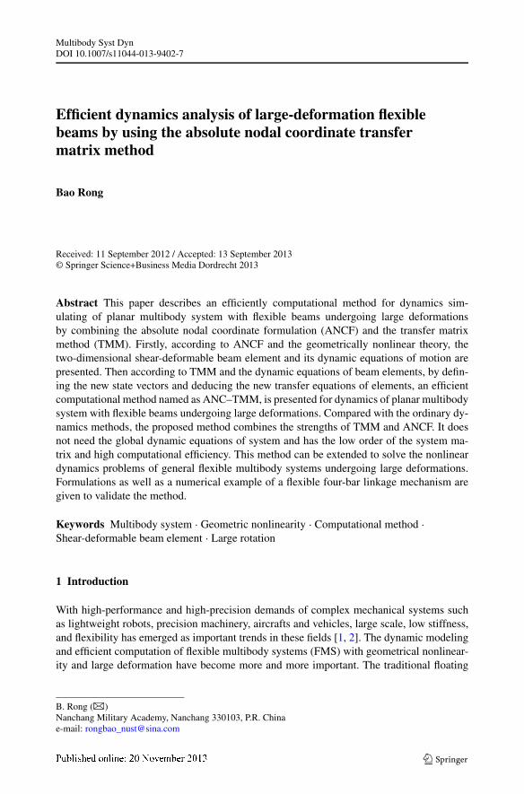
In this section, the numerical simulation of the four-bar mechanism shown in Fig. 1 is pre-sented. The crankshaft is derived by a servo system, and its orientation angle as a functionof time is presented in Fig. 5. The inertia, geometric, and elastic properties of the compo-nents of the four-bar mechanism are shown in Table 1. The table shows the mass m, thecross-sectional area A, the second moment of area I , the length l, and the modulus of elas-ticity E of the mechanism components. The initial orientation of the crankshaft is zero. Thecrankshaft, a coupler and a follower, are divided into two, eight, and two finite elements,respectively.
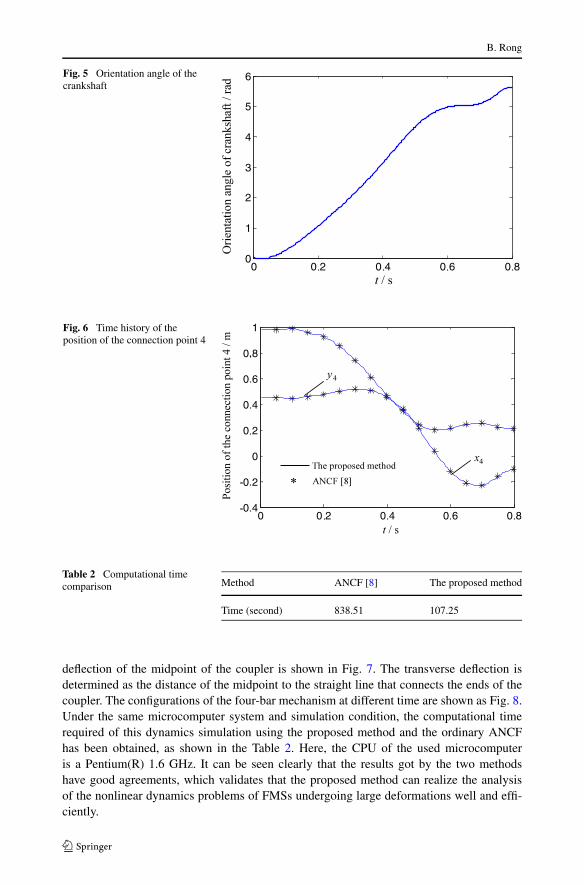
The dynamics of this system are computed by solving the transfer equation (35) de-duced by the proposed method and by direct explicitly integrating the global dynamic equa-tion (14) of the systems deduced by the ANCF [8], respectively. The time history of theposition of the connection point 4 got by the two methods is shown in Fig. 6. The transverse
B. Rong
Fig. 5 Orientation angle of thecrankshaft
Fig. 6 Time history of theposition of the connection point 4
Table 2 Computational timecomparison Method ANCF [8] The proposed method
Time (second) 838.51 107.25
deflection of the midpoint of the coupler is shown in Fig. 7. The transverse deflection isdetermined as the distance of the midpoint to the straight line that connects the ends of thecoupler. The configurations of the four-bar mechanism at different time are shown as Fig. 8.Under the same microcomputer system and simulation condition, the computational timerequired of this dynamics simulation using the proposed method and the ordinary ANCFhas been obtained, as shown in the Table 2. Here, the CPU of the used microcomputeris a Pentium(R) 1.6 GHz. It can be seen clearly that the results got by the two methodshave good agreements, which validates that the proposed method can realize the analysisof the nonlinear dynamics problems of FMSs undergoing large deformations well and effi-ciently.
Efficient dynamics analysis of large-deformation flexible beams by using
Fig. 7 Transverse deflection ofthe midpoint of the coupler
Fig. 8 Configurations of the four-bar mechanism at different time
6 Conclusions
In this paper, by combining the ANCF and TMM, a new efficient computational methodnamed as ANC–TMM is presented for dynamics simulating of planar multibody system withflexible beams undergoing large deformations. Formulations as well as a numerical exampleof a flexible four-bar linkage mechanism are given to validate the method. Compared withthe ordinary dynamics methods, the proposed method combines the strengths of TMM andANCF, and has the following advantages: (1) The global dynamic equations of system arenot needed, which simplifies the dynamic modeling and the solution procedure of flexiblemultibody systems. (2) Irrespective of the size of a system, the matrices involved in thismethod are always small, which greatly reduces the computational time and memory storagerequirement. (3) This method can be extended to solve the nonlinear dynamics problems ofgeneral flexible multibody systems undergoing large deformations.
B. Rong
In this paper, an explicit numerical integration method is used. For the dynamics prob-lems of flexible multibody systems with large deformation, the conditional convergence ofthe explicit numerical integration method usually restricts the integration step size, whichwill increase the computational cost on the other hand. Sometimes the computational stabil-ity is also put on trial. How to using an implicit numerical integration method in ANC–TMMto improve the computational stability and computational efficiency of dynamics analysiswill be discussed in the following paper.
Acknowledgements The research was supported by the Natural Science Foundation of China Govern-ment (Grant No. 10902051) and the Program for New Century Excellent Talents in University (Grant No.NCET-10-0075). We owe special thanks to Professor Jorge A.C. Ambrósio (Instituto Superior Técnico, Lis-bon, Portugal) and Professor Werner Schiehlen (University of Stuttgart, Germany) for their heuristic sugges-tions.
References
1. Schiehlen, W.: Research trends in multibody system dynamics. Multibody Syst. Dyn. 18(1), 3–13 (2007)2. Wasfy, T.M., Noor, A.K.: Computational strategies for flexible multibody system. Appl. Mech. Rev.
56(6), 553–613 (2003)3. Shabana, A.A.: Dynamics of Multibody Systems. Cambridge University Press, New York (2005)4. Berzeri, M., Campanelli, M., Shabana, A.A.: Definition of the elastic forces in the finite-element absolute
nodal coordinate formulation and the floating frame of reference formulation. Multibody Syst. Dyn. 5(1),21–54 (2001)
5. Omar, M.A., Shabana, A.A.: A two-dimensional shear deformable beam for large rotation and deforma-tion problems. J. Sound Vib. 243(3), 565–576 (2001)
6. Matikainen, M.: Development of beam and plate finite elements based on the absolute nodal coordinateformulation. Ph.D. dissertation, Lappeenranta University of Technology, Finland (2009)
7. Tian, Q., Zhang, Y.Q., Chen, L.P., Qin, G.: Advances in the absolute nodal coordinate method for theflexible multibody dynamics. Adv. Mech. 40(2), 189–202 (2010)
8. García-Vallejo, D., Mayo, J., Escalona, J.L., Domínguez, J.: Efficient evaluation of the elastic forces andthe Jacobian in the absolute nodal coordinate formulation. Nonlinear Dyn. 35, 313–329 (2004)
9. Gerstmayr, J., Shabana, A.A.: Efficient integration of the elastic forces and thin three-dimensional beamelements in the absolute nodal coordinate formulation. In: ECCOMAS Thematic Conference, Madrid,Spain, 21–24 June 2005, pp. 21–24 (2005)
10. Liu, C., Tian, Q., Hu, H.Y.: Efficient computational method for dynamics of flexible multibody systemsbased on absolute nodal coordinate. Theor. Appl. Mech. Lett. 42(6), 1197–1204 (2010)
11. Yakoub, R.Y., Shabana, A.A.: Use of Cholesky coordinates and the absolute nodal coordinate formula-tion in the computer simulation of flexible multibody systems. Nonlinear Dyn. 20(3), 267–282 (1999)
12. Chijie, L.: Dynamic and thermal analyses of flexible structures in orbit. Ph.D. dissertation, University ofConnecticut, Storrs (2006)
13. Pestel, E.C., Leckie, F.A.: Matrix Method in Elastomechanics. McGraw-Hill, New York (1963)14. Kumar, A.S., Sankar, T.S.: A new transfer matrix method for response analysis of large dynamic systems.
Comput. Struct. 23(4), 545–552 (1986)15. Dokanish, M.A.: A new approach for plate vibration: combination of transfer matrix and finite element
1052 (1999)17. Xue, H.Y.: A combined finite element-stiffness equation transfer method for steady state vibration re-
sponse analysis of structures. J. Sound Vib. 265(4), 783–793 (2003)18. Rong, B., Rui, X.T., Wang, G.P., et al.: Modified finite element transfer matrix method for eigenvalue
problem of flexible structures. J. Appl. Mech. 78(2), 021016 (2011)19. Rong, B., Rui, X.T., Wang, G.P.: New method for dynamics modeling and analysis on flexible plate
undergoing large overall motion. Proc. Inst. Mech. Eng., Proc., Part K, J. Multi-Body Dyn. 224(K1),33–44 (2010)
20. Rong, B., Rui, X.T., Wang, G.P., et al.: New efficient method for dynamics modeling and simulation offlexible multibody systems moving in plane. Multibody Syst. Dyn. 24(2), 181–200 (2010)
Efficient dynamics analysis of large-deformation flexible beams by using
21. Horner, G.C.: The Riccati transfer matrix method. Ph.D. dissertation, University of Virginia, USA(1975)
22. Wang, G.P., Rong, B., Tao, L., Rui, X.T.: Riccati discrete time transfer matrix method for dynamicmodeling and simulation of an underwater towed system. J. Appl. Mech. 79(4), 041014 (2012)
23. Zhai, W.M.: Two simple fast integration methods for large-scale dynamic problems in engineering. Int.J. Numer. Methods Eng. 39(24), 4199–4214 (1996)